Building water bridges in air: Electrohydrodynamics of the Floating Water Bridge

Alvaro G. Marın and Detlef LohsePhysics of Fluids, University of Twente

(Dated: October 20, 2010)

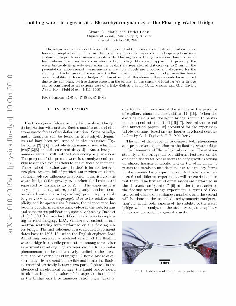
The interaction of electrical fields and liquids can lead to phenomena that defies intuition. Somefamous examples can be found in Electrohydrodynamics as Taylor cones, whipping jets or non-coalescing drops. A less famous example is the Floating Water Bridge: a slender thread of waterheld between two glass beakers in which a high voltage difference is applied. Surprisingly, thewater bridge defies gravity even when the beakers are separated at distances up to 2 cm. In thepresentation, experimental measurements and simple models are proposed and discussed for thestability of the bridge and the source of the flow, revealing an important role of polarization forceson the stability of the water bridge. On the other hand, the observed flow can only be explaineddue to the non negligible free charge present in the surface. In this sense, the Floating Water Bridgecan be considered as an extreme case of a leaky dielectric liquid (J. R. Melcher and G. I. Taylor,Annu. Rev. Fluid Mech., 1:111, 1969).

PACS numbers: 47.65.-d, 47.55.nk, 47.20.Ma

I. INTRODUCTION

Electromagnetic fields can only be visualized throughits interaction with matter. Such a manifestation of elec-tromagnetic forces often defies intuition. Some paradig-matic examples can be found in Electrohydrodynam-ics and have been well studied in the literature: Tay-lor cones [2][5][6], electrohydrodynamic driven whippingjets[7][3][8] or anti-coalescent drops[4]. But a few phe-nomena remain still without convincing explanations.The purpose of the present work is to analyze and pro-vide reasonable explanations to one of these phenomena:The so-called “floating water bridge” is formed betweentwo glass beakers full of purified water when an electri-cal high voltage difference is applied. Surprisingly, thewater bridge defies gravity even when the beakers areseparated by distances up to 2cm. The experiment iseasy enough to reproduce, needing only standard dem-ineralized water and a high voltage power supply (ableto give 20kV at low amperage). Due to its relative sim-plicity and its spectacular features, the phenomenon hasbecome popular in science fairs, videos in the web, forumsand some recent publications, specially those by Fuchs etal. [9][10][11][12], in which different experiments employ-ing thermal imaging, LDA, Schlieren visualization andneutron scattering were performed on the floating wa-ter bridge. The first reference of a controlled experimentdates back to 1893 [13], when the English engineer LordArmstrong presented a modified version of the floatingwater bridge in a public presentation, among some otherexperiments involving high voltages and fluids. A similarphenomenon has been intensively studied in the litera-ture, the “dielectric liquid bridge”: A liquid bridge of oil,surrounded by a second immiscible and insulating liquid,is sustained vertically between two parallel plates, in theabsence of an electrical voltage, the liquid bridge wouldbreak into droplets for values of the aspect ratio (definedas the bridge length to diameter ratio) higher than π,

due to the minimization of the surface in the presenceof capillary sinusoidal instabilities [14] [15]. When theelectrical field is set, the liquid bridge is found to be sta-ble for aspect ratios up to 6 [16][17]. Several theoreticaland numerical papers [18] accounted for the experimen-tal observations, based on the theories developed decadesbefore by G. I. Taylor & J. R. Melcher[7].

The aim of this paper is to connect both phenomenaand propose an explanation to the floating water bridgein the framework of Electrohydrodynamics. The strikingstability of the bridge has two different features: on theone hand the water bridge seems to defy gravity showingan almost horizontal profile, and on the other hand, itresists the break-up into droplets due to capillary forcesuntil extremely large aspect ratios. Both effects are con-nected and different experiments will be carried out totest them. The first set of experiments are performed inthe “beakers configuration” [9] in order to characterizethe floating water bridge experiment in terms of Elec-trohydrodynamic dimensionless numbers, and the secondwill be done in the so called “axisymmetric configura-tion”, in which both aspects of the stability of the waterbridge will be analyzed: the stability against capillaryforces and the stability against gravity.

FIG. 1. Side view of the Floating water bridge

arX

iv:1

010.

4019

v1 [

phys

ics.

flu-

dyn]

19

Oct

201

0

2

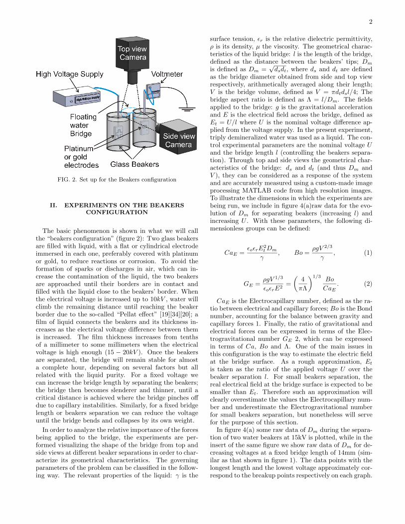
FIG. 2. Set up for the Beakers configuration

II. EXPERIMENTS ON THE BEAKERSCONFIGURATION

The basic phenomenon is shown in what we will callthe “beakers configuration” (figure 2): Two glass beakersare filled with liquid, with a flat or cylindrical electrodeimmersed in each one, preferably covered with platinumor gold, to reduce reactions or corrosion. To avoid theformation of sparks or discharges in air, which can in-crease the contamination of the liquid, the two beakersare approached until their borders are in contact andfilled with the liquid close to the beakers’ border. Whenthe electrical voltage is increased up to 10kV , water willclimb the remaining distance until reaching the beakerborder due to the so-called “Pellat effect” [19][34][20]; afilm of liquid connects the beakers and its thickness in-creases as the electrical voltage difference between themis increased. The film thickness increases from tenthsof a millimeter to some millimeters when the electricalvoltage is high enough (15 − 20kV ). Once the beakersare separated, the bridge will remain stable for almosta complete hour, depending on several factors but allrelated with the liquid purity. For a fixed voltage wecan increase the bridge length by separating the beakers;the bridge then becomes slenderer and thinner, until acritical distance is achieved where the bridge pinches offdue to capillary instabilities. Similarly, for a fixed bridgelength or beakers separation we can reduce the voltageuntil the bridge bends and collapses by its own weight.

In order to analyze the relative importance of the forcesbeing applied to the bridge, the experiments are per-formed visualizing the shape of the bridge from top andside views at different beaker separations in order to char-acterize its geometrical characteristics. The governingparameters of the problem can be classified in the follow-ing way. The relevant properties of the liquid: γ is the

surface tension, εr is the relative dielectric permittivity,ρ is its density, µ the viscosity. The geometrical charac-teristics of the liquid bridge: l is the length of the bridge,defined as the distance between the beakers’ tips; Dm

is defined as Dm =√dsdt, where ds and dt are defined

as the bridge diameter obtained from side and top viewrespectively, arithmetically averaged along their length;V is the bridge volume, defined as V = πdtdsl/4; Thebridge aspect ratio is defined as Λ = l/Dm. The fieldsapplied to the bridge: g is the gravitational accelerationand E is the electrical field across the bridge, defined asEt = U/l where U is the nominal voltage difference ap-plied from the voltage supply. In the present experiment,triply demineralized water was used as a liquid. The con-trol experimental parameters are the nominal voltage Uand the bridge length l (controlling the beakers separa-tion). Through top and side views the geometrical char-acteristics of the bridge: ds and dt (and thus Dm andV ), they can be considered as a response of the systemand are accurately measured using a custom-made imageprocessing MATLAB code from high resolution images.To illustrate the dimensions in which the experiments arebeing run, we include in figure 4(a)raw data for the evo-lution of Dm for separating beakers (increasing l) andincreasing U . With these parameters, the following di-mensionless groups can be defined:

CaE =εoεrE

2tDm

γ, Bo =

ρgV 2/3

γ, (1)

GE =ρgV 1/3

εoεrE2=

(4

πΛ

)1/3Bo

CaE. (2)

CaE is the Electrocapillary number, defined as the ra-tio between electrical and capillary forces; Bo is the Bondnumber, accounting for the balance between gravity andcapillary forces 1. Finally, the ratio of gravitational andelectrical forces can be expressed in terms of the Elec-trogravitational number GE 2, which can be expressedin terms of Ca, Bo and Λ. One of the main issues inthis configuration is the way to estimate the electric fieldat the bridge surface. As a rough approximation, Et

is taken as the ratio of the applied voltage U over thebeaker separation l. For small beakers separation, thereal electrical field at the bridge surface is expected to besmaller than Et. Therefore such an approximation willclearly overestimate the values the Electrocapillary num-ber and underestimate the Electrogravitational numberfor small beakers separation, but nonetheless will servefor the purpose of this section.

In figure 4(a) some raw data of Dm during the separa-tion of two water beakers at 15kV is plotted, while in theinsert of the same figure we show raw data of Dm for de-creasing voltages at a fixed bridge length of 14mm (sim-ilar as that shown in figure 1). The data points with thelongest length and the lowest voltage approximately cor-respond to the breakup points respectively on each graph.

3

FIG. 3. First row of images: Different side views during sepa-ration of the beakers. Second row: Different top views duringseparation of the beakers. Nominal voltage 15kV. The scalebars have a length of 10mm; in the right images, the bridgereaches an aspect ratio Λ ≈ 10.

FIG. 4. Measurements in the beakers configuration: a)rawdata for Dm as a function of the beaker separation l, and as afunction of the applied voltage U (insert). b) Electrocapillarynumber Ca vs the aspect ratio Λ during the separation of thebeakers. c) Electrogravitational number GE vs the aspectratio Λ. d) Bond number Bo vs the aspect ratio Λ during theseparation of the beakers.

Although the electrical current has not been shown forclearness in this last experiment, we should mention thatit decreases linearly for decreasing voltages from valuesof order 0.8mA to nearly zero when the bridge collapses.Since the current passing through the bridge is clearlynon-negligible, the bridge suffers Joule heating. However,the experiments shown in figure 4 were performed nor-mally in short sessions of maximum 5 min, after whichthe water was replaced. The measured temperature atthe end of each short session was close to 45℃ (113◦F),this would imply an error in the surface tension of around4%. For a fixed voltage U and increasing beaker distancesl, the values of these dimensionless numbers are plottedin figures ??(b) to (c). As can be seen in figure 4(b), theElectrocapillary number CaE decreases until values stillabove unity in the breakup point, in figure 4(c) the Elec-trogravitational number GE increases, but remains well

below unity during the whole process, and finally in figure4(d) the Bond number Bo and the Electrocapillary num-ber CaE decrease until the bridge collapses with Bondnumbers well below unity. This shows us that the initialstage of the bridge (left column in figure 3) is dominatedby Electrical forces, with negligible effect of the capil-lary forces and gravity. In contrast, in the late stageswhen the bridge becomes thinner (right column in figure3) there seems to be a delicate balance of electrical andcapillary forces, and therefore the Electrocapillary num-ber is the most relevant number in the most elongatedbridges.

From this point of view, this last stage shares similarcharacteristics with the classical work on dielectric liquidbridges under electrical fields [16][18]. The shown resultsare interesting to identify the main forces, but in orderto proceed with a more detailed analysis one must beable to determine more precisely the electric field close tothe bridge interface. For this reason, the “Axisymmetricconfiguration” is employed in the following, in which thestruggle of the electrical forces against capillarity andgravity are studied.

III. AXISYMMETRIC CONFIGURATION:STABILITY AGAINST CAPILLARY FORCES

The stabilization of dielectric liquid cylinders underthe action of a longitudinal electrical fields have beenstudied theoretically-numerically [21] [18] and experi-mentally [16] [17]. The underlying physics are based oninduced polarization forces on dielectrics [22] [23]: in apure dielectric liquid cylinder under an electrical fieldapplied parallel to its interface, any sinusoidal perturba-tion developed over its surface would create polarizationcharges of opposite signs in different slopes that will tendto stabilize the surface. On the other hand, for electri-cally conducting liquids, the charge in semi-equilibriumover the surface makes the picture much more compli-cated and the equilibrium is no longer guaranteed. Sinceliquids in nature are neither pure conductors nor puredielectrics, Taylor and Melcher developed the so called“leaky dielectric model”[1] [24] in which a dielectric liquidis assumed to have some free charge that only manifestsat its surface. Such a model was applied to a leaky di-electric liquid cylinder under a longitudinal electrical fieldby Saville [18], concluding that surface charge transportwould lead to a charge redistribution and a consequentinstability of the liquid cylinder. A similar but not com-parable result[25] was found on infinite jets: unstablebut oscillatory modes were found as the charge relax-ation effects, i.e. the ability of the free charge to find itsequilibrium on the surface, were increased.

Therefore, if the induced polarization forces are re-sponsible for the stability of the liquid bridge, less electri-cal voltage U will be needed to maintain a liquid bridgeas the dielectric permittivity εr of the liquid increases. Inorder to test such an effect, an axisymmetric set up was

4

TABLE I. Properties of the employed liquids

LiquidDensityρ (kg/m3)

SurfaceTensionγ (mN/m)

DynamicViscosityµ (mPa · s)

DielectricConstantεr

ElectricalConductivityK (µS/cm)

Glycerine 1250 64 1050 41.6 0.01575%w Glycerine- 25%w water 1182 66 31 54.7 0.21350%w Glycerine- 50%w water 1115 68 5 65.6 0.560Ultrapure millipore water 980 72 1 81 0.520

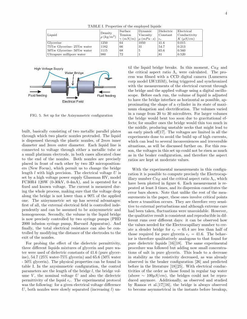
FIG. 5. Set up for the Axisymmetric configuration

built, basically consisting of two metallic parallel platesthrough which two plastic nozzles protruded. The liquidis dispensed through the plastic nozzles, of 2mm innerdiameter and 3mm outer diameter. Each liquid line isconnected to voltage through either a metallic tube ora small platinum electrode, in both cases allocated closeto the end of the nozzles. Both nozzles are preciselyplaced in front of each other by two 3D microposition-ers (New Focus), which permit us to change the bridgelength l with high precision. The electrical voltage U isset by a high voltage power supply Glassman HV, modelFC30R4 120W (0-30kV, 0-4mA), and is operated for afixed and known voltage. The current is measured dur-ing the whole process, making sure that the voltage dropalong the bridge is not lower than a 90% of the appliedone. The axisymmetric set up has several advantages:first of all, the external electrical field is controlled inde-pendently and can be assumed to be axisymmetric andhomogeneous. Secondly, the volume in the liquid bridgeis now precisely controlled by two syringe pumps (PHD2000 infusion syringe pump, Harvard Apparatus). Andfinally, the total electrical resistance can also be con-trolled by modifying the distance of the electrodes to theexit of the nozzles.

For probing the effect of the dielectric permittivity,three different liquids mixtures of glycerin and pure wa-ter were used of dielectric constants of 41.6 (pure glycer-ine), 54.7 (25% water-75% glycerin) and 65.6 (50% water- 50% glycerin). The physical properties can be found intable I. In the axysimmetric configuration, the controlparameters are the length of the bridge l, the bridge vol-ume V , the nominal voltage U and also the dielectricpermittivity of the liquid εr. The experimental protocolwas the following: for a given electrical voltage differenceU , both nozzles were slowly separated (increasing l) un-

til the liquid bridge breaks. In this moment, CaE andthe critical aspect ratio Λc were calculated. The pro-cess was filmed with a CCD digital camera (Lumeneracorp model LW135M), being triggered and synchronizedwith the measurements of the electrical current throughthe bridge and the applied voltage using a digital oscillo-scope. Before each run, the volume of liquid is adjustedto have the bridge interface as horizontal as possible, ap-proximating the shape of a cylinder in its state of maxi-mum elongation and electrification. The volumes variedin a range from 20 to 30 microliters. For larger volumesthe bridge would bent too soon due to gravitational ef-fects; for smaller ones the bridge would thin too much inthe middle, producing unstable necks that might lead toan early pinch off[17]. The voltages are limited in all theexperiments done to avoid the build up of high currents,which can lead to several inconveniences and irreversiblesituations, as will be discussed further on. For this rea-son, the voltages in this set up could not be risen as muchas in the beaker configuration, and therefore the aspectratios are kept at moderate values.

With the experimental measurements in this configu-ration it is possible to compute precisely the Electrocap-illary number CaE and the critical aspect ratio Λc, whichhave been plotted in figure 6. Each measurement is re-peated at least 3 times, and its dispersion constitutes theerror bars shown. Note that unlike the rest of the mea-surements in the paper, these ones involve critical pointswhere a transition occurs. They are therefore very sensi-tive to external perturbations and although extreme carehad been taken, fluctuations were unavoidable. However,the qualitative result is consistent and reproducible in dif-ferent runs over different days: it can be observed howthe values needed for the Electrocapillary number to cre-ate a slender bridge for εr = 65.4 are less than half ofthose required for pure glycerin εr = 41.6. The behav-ior is therefore qualitatively analogous to that found forpure dielectric liquids [16][18]. The same experimentalprocedure was followed but adding now small concentra-tions of salt in pure glycerin. This leads to a decreasein stability as the resistivity decreased, as was alreadyobserved in the beaker configuration [26] and predictedbefore in the literature [18][25]. With electrical conduc-tivities of the order as those found in regular tap water(above ∼ 100µS/cm), the bridges could not be repro-duced anymore. Additionally, as observed and studiedby Ramos et al.[17][16], the bridge is always observedto become asymmetrical in the instants before breakup,

5

FIG. 6. Electrocapillary number CaE vs the critical aspectratio Λc = lc/Dm at which the bridge breaks for a fixed volt-age and slowly increasing l.

with a more prominent bulb on one side than the other.

Some drawbacks need to be mentioned concerning theexperimental results: In an ideal case without gravityand without wetting effects, the liquid cylinder at zerovoltage should have a maximum aspect ratio of value π,according to the Plateau criterium [15]. However, due togravity and wetting effects, the aspect ratios found in theabsence of electric voltage are much lower than those ide-ally expected [17] [18], namely around 2.4 rather than π.Secondly, as was already observed in the beaker configu-ration, hydrogen bubbles are generated at the cathodesurface when water-based liquids are used, evidencingthe presence of electrolysis in the process, specially whenhigher currents are generated. This is not an issue in thebeaker configuration, where larger volumes of liquid areemployed and more surface is exposed to air, hence thebubbles rise to the liquid surface and only rarely theyenter into the bridge. In the case of the axisymmetricconfiguration, covering the electrodes with platinum foilreduced the problem, but did not solve it completely, andbubbles were still generated as the percentage of waterand the voltages increased. For this reason, the max-imum percentage of water used in the experiments was50% and the voltages were limited to avoid high currents.Joule heating can be safely neglected in these cases, sincethe electrical conductivity is reduced significantly as wellas the thermal conductivity of the water/glicerine mix-tures as compared with the experiments in section . An-other issue to have in mind involves the relative impor-tance of gravitational forces in this whole process. Al-though it has been shown that the Bond numbers aresmall in these stages, they can not be completely ne-glected. Several efforts were done in the past to avoidthis effect by using density matching techniques[16] orparabolic flights to perform the experiments in micro-gravity conditions [27]. Finally, the last issue was al-ready mentioned by Melcher and Taylor in the abstractof their pioneering review [1], and it concerns the con-

trol in polar liquids of the electrical conductivity. Polarliquids are more prone to become contaminated, even inthis set up in which they were confined avoiding the con-tact with contaminants. For this reason, glycerin waschosen as base liquid, and permitted us to achieve morereproducible results. It has been necessary to employthe axisymmetric configuration and different liquids toisolate the dielectric effects from the rest, although the“floating water bridge” effect is not as impressive as itwas in the beaker configuration due to the mentionedreasons.

Nonetheless, within the aforementioned limitations, wecan conclude that induced dielectric polarization is re-sponsible for the stability against capillary collapse inthe water bridge through the mechanism described atthe beginning of this section. There are still several mat-ters to be clarified: first of all, the role of charge relax-ation effects on the instability of the bridge. It has beendemonstrated that the increase of free charge (electri-cal conductivity) certainly disturbs the equilibrium, aswas also shown by Burcham & Saville [18] in bridges ofdielectric liquids. But, how disturbing can this be? Tak-ing water as a purely dielectric liquid (no free charge)of εr = 81 and performing a simple stability analysis asthat performed by Nayyar & Murty [21], with CaE ≈ 1,the analysis yields aspect ratios of Λ ≈ 100 (taking forthe maximum length of the bridge the maximum unsta-ble wavelength). In contrast, the highest aspect ratiosobserved experimentally rarely reach values of 10 (rightimages in figure 3). According to this line of reasoninga non trivial question arises: why is the effect not ob-served with dielectric bridges in which the free chargecan be almost neglected (e.g. oils)? Recurring again tothe stability analysis for a dielectric liquid of εr = 2 anda diameter of 2mm held in air, even for the maximumelectrical fields that can be achieved in our system be-fore air breakdown (some kV per mm), only small aspectratios are obtained, hardly 5% higher than the valuesexpected in the absence of electrical field [24]. This factmanifests the high dependance of the phenomenon on thedielectric permittivity of the liquid, which is unavoidablyconnected with the amount of free charge that can be dis-solved in the liquid.

The effect of the electrical shear stresses on the sta-bility of the bridge deserves also some comments. It iswell known that a strong shear over an interface can beused to stabilize liquid jets [28][29][7] [30]. In these citedcases the electrical current is driven by convection andtherefore is independent of the downstream conditions.Charge is well separated before reaching the jet[5], andis forced to be transported only in the direction of theflow, under strong surface shear stresses and high accel-erations, achieving supercritical regimes[30]. However,for the case of liquid bridges the charge transport is onlydue to conduction, charge of opposite signs coexist in thesystem and the electrical shear stresses are nonuniformlyand unsteadily distributed along the bridge, giving riseto the complicated flow patterns. In this sense, the con-

6

ditions and the characteristics of the liquid bridge wouldresemble those of the “decelerating stream”, depicted andanalyzed by Melcher & Warren [30].

IV. AXISYMMETRIC CONFIGURATION:STABILITY AGAINST GRAVITY.

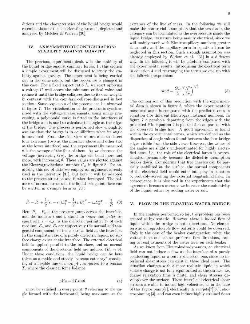
The previous experiments dealt with the stability ofthe liquid bridge against capillary forces. In this sectiona simple experiment will be discussed to study the sta-bility against gravity. The experiment is being carriedout in the same setup, but the procedure is changed inthis case. For a fixed aspect ratio Λ, we start applyinga voltage U well above the minimum critical value andreduce it until the bridge collapses due to its own weight,in contrast with the capillary collapse discussed in lastsection. Some sequences of the process can be observedin figure 7. The visualization of the process is synchro-nized with the voltage measurements, using image pro-cessing, a polynomial curve is fitted to the interfaces ofthe bridge and is used to calculate the angle at the edgesof the bridge. The process is performed slow enough toassume that the bridge is in equilibrium when its angleis measured. From the side view we are able to detectfour extremes (two at the interface above and other twoat the lower interface) and the experimentally measuredθ is the average of the four of them. As we decrease thevoltage (increasing GE), the bridge will bend more andmore, with increasing θ. These values are plotted againstthe Electrogravitational number GE in figure 8. For an-alyzing this set of data we employ an argument alreadyused in the literature [31], but here it will be adaptedto the present situation and further developed. The bal-ance of normal stresses in the liquid bridge interface canbe written in a simple form as [23]:

Pi − Po +1

2(εi − εo)E2

t −1

2(εiE

in

2 − εoEon2) =

γ

R(3)

Here Pi − Po is the pressure jump across the interface,and the indexes i and o stand for inner and outer re-spectively, ε = εoεr is the dielectric permittivity of eachmedium, En and Et are respectively the normal and tan-gential components of the electrical field at the interface.In the simplistic case of a purely dielectric liquid, no sur-face charge exists at the interface. The external electricalfield is applied parallel to the interface, and no normalcomponents of the electrical field are induced (En ≈ 0).Under these conditions, the liquid bridge can be heretaken as a stable and steady “viscous catenary” consist-ing of a flexible line of mass ρV , subjected to a tensionT , where the classical force balance

ρV g = 2Tsinθ (4)

must be satisfied in every point, θ referring to the an-gle formed with the horizontal, being maximum at the

extremes of the line of mass. In the following we willmake the non-trivial assumption that the tension in thecatenary can be formulated as the overpressure inside theliquid bridge, its nature being mainly electrical, since wewill mainly work with Electrocapillary numbers greaterthan unity and the capillary term in equation 3 can beneglected in this section. Such a rough assumption wasalready employed by Widom et al. [31] in a differentway. In the following it will be carefully compared withthe experimental results. Introducing the electrical termin equation 4 and rearranging the terms we end up withthe following expression:

sinθ =GE

2

(Λ2

2π

)1/3

(5)

The comparison of this prediction with the experimen-tal data is shown in figure 8, where the experimentallymeasured angle is compared with the predicted ones inequation 4for different Electrogravitational numbers. Infigure 7 a parabola departing from the edges with thepredicted θ in equation 4 is plotted for comparison withthe observed bridge line. A good agreement is foundwithin the experimental errors, which are defined as thedispersion of angle values found between the four bridgeedges visible from the side view. However, the values ofthe angles are slightly underestimated for highly electri-fied cases, i.e. the role of the electrical forces is overes-timated, presumably because the dielectric assumptionbreaks down. Considering that free charges can be par-tially stabilized at the surface, the normal componentsof the electrical field would enter into play in equation5, probably screening the external longitudinal field. Inconsequence, it is observed in the experiments that theagreement becomes worse as we increase the conductivityof the liquid, either by adding water or salt.

V. FLOW IN THE FLOATING WATER BRIDGE

In the analysis performed so far, the problem has beentreated as hydrostatic. However, there is indeed flow ofliquid within the bridge in both directions. No charac-teristic or reproducible flow patterns could be observed.Only in the case of the beaker configuration, when thevoltage is set one can see preferred flow directions, lead-ing to readjustments of the water level on each beaker.

As we know from Electrohydrodynamics, an electricalfield can not induce a flow at the interface of a purelyconducting liquid or a purely dielectric one, since no in-terfacial shear stress can exist in these ideal cases. Thesituation changes with a more realistic liquid in whichsurface charge is not fully equilibrated at the surface, i.e.charge relaxation time is finite, and shear stresses de-velop over the surface. These interfacial electrical shearstresses are able to induce high velocities, as in the caseof the Taylor pump[1], electrically driven jets[7][30], elec-trospinning [3], and can even induce highly strained flows

7

FIG. 7. Different side views of a glycerine bridge for decreasing voltages (increasing Electrogravitational numbers GE), fromleft to right: GE = 0.2, 0.8 and 1. A line outlines the liquid surface and the line departing from the middle of the nozzle depictsa parabola with the predicted θ at the nozzle. The nozzles diameter is 3 mm.

FIG. 8. Angle at the edge θ of the ‘catenary bridge’ vs theElectrogravitational numberGE , the straight line correspondsto the prediction in equation 5.

able to generate geometrical singularities in droplets [32].Such shear stress depends linearly on the tangential fieldat the interface and on the surface charge induced at theinterface. Here we face a common problem in Electro-hydrodynamics: Only in very few paradigmatic experi-ments the surface charge can be properly modeled andindirectly determined, as in the case of the Taylor pump[1][33]. In the particular case of a liquid bridge, Bur-cham and Saville [18] numerically solved the problem fora leaky dielectric, introducing the surface conductivityas a free parameter and they found an heterogenous dis-tribution of charge at the bridge surface, which in theircase gave rise to a recirculating flow pattern.

In our case, the distribution of the surface charge andits stability is quite unclear, but according to the con-clusions of the last sections, it seems that surface chargeis not fully in equilibrium at the surface. Therefore, theelectrical shear stress generated must be quite unsteadyand inhomogeneous, giving rise to strong spatial and tem-poral variations in the velocity fields, even giving the im-pression to be chaotic. However, the temporal scale in

which such flow patterns change can be of the order ofseconds. This fact permitted to measure the interfacialvelocity by using high speed cameras and perform Par-ticle Image Velocimetry in an area close to the surface,combined with Particle Tracking Velocimetry in thosecases where the particle density was too reduced.

In order to give a rough prediction on the velocitiesin the bridge we need an estimate of the electrical shearstress generated at the surface. The balance of shearstresses at the interface can be expressed as follows:

qsEt = µ∂us∂y

(6)

where qs refers to the surface charge density, Et to thetangential field at the surface, µ to the liquid viscosityand us the surface velocity. The surface charge densityqs = εoE

on − εiEi

n would acquire its maximum value forthe perfectly conducting case, in such a case qos = εoE

on

and the surface charge would remain in perfect equilib-rium. Unfortunately, nothing can be said a priori aboutsurface charge but qs << qos , as has been argued in previ-ous sections. Therefore, us and qs can not be estimatedindependently. To get a better insight into this matter,the following magnitudes ratios are defined:

Φ =Ei

n

Eon

(7)

Ξ =Eo

n

Et(8)

With this definition Ξ express the relative importanceof the normal electrical field components against the tan-gential ones, responsable for the shear stress. And Φ goesto zero for perfectly conducting liquids, in which chargeis stable at the interface and no shear stress can exists.Moreover, surface velocity can be expressed in dimension-less units making use of the capillary velocity uo = γ/µand the Electrocapillary number CaE . With these intro-duced definitions, the induced velocities at the interfacecan be written as:

8

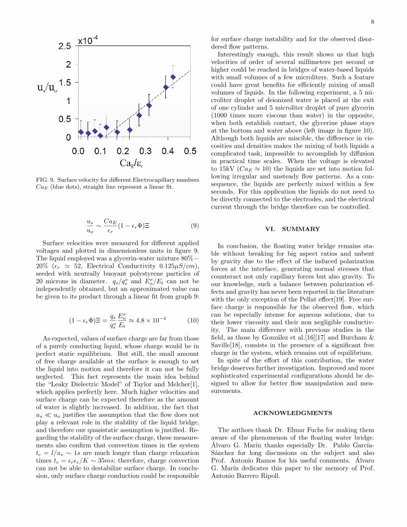
FIG. 9. Surface velocity for different Electrocapillary numbersCaE (blue dots), straight line represent a linear fit.

usuo∼ CaE

εr(1− εrΦ)Ξ (9)

Surface velocities were measured for different appliedvoltages and plotted in dimensionless units in figure 9.The liquid employed was a glycerin-water mixture 80%−20% (εr ' 52, Electrical Conductivity 0.125µS/cm),seeded with neutrally buoyant polystyrene particles of20 microns in diameter. qs/q

os and Eo

n/Et can not beindependently obtained, but an approximated value canbe given to its product through a linear fit from graph 9:

(1− εrΦ)Ξ =qsqos

Eon

Et≈ 4.8× 10−4 (10)

As expected, values of surface charge are far from thoseof a purely conducting liquid, whose charge would be inperfect static equilibrium. But still, the small amountof free charge available at the surface is enough to setthe liquid into motion and therefore it can not be fullyneglected. This fact represents the main idea behindthe “Leaky Dielectric Model” of Taylor and Melcher[1],which applies perfectly here. Much higher velocities andsurface charge can be expected therefore as the amountof water is slightly increased. In addition, the fact thatus � uo justifies the assumption that the flow does notplay a relevant role in the stability of the liquid bridge,and therefore our quasistatic assumption is justified. Re-garding the stability of the surface charge, these measure-ments also confirm that convection times in the systemtc = l/us ∼ 1s are much longer than charge relaxationtimes tc = εrεc/K ∼ 35ms; therefore, charge convectioncan not be able to destabilize surface charge. In conclu-sion, only surface charge conduction could be responsible

for surface charge instability and for the observed disor-dered flow patterns.

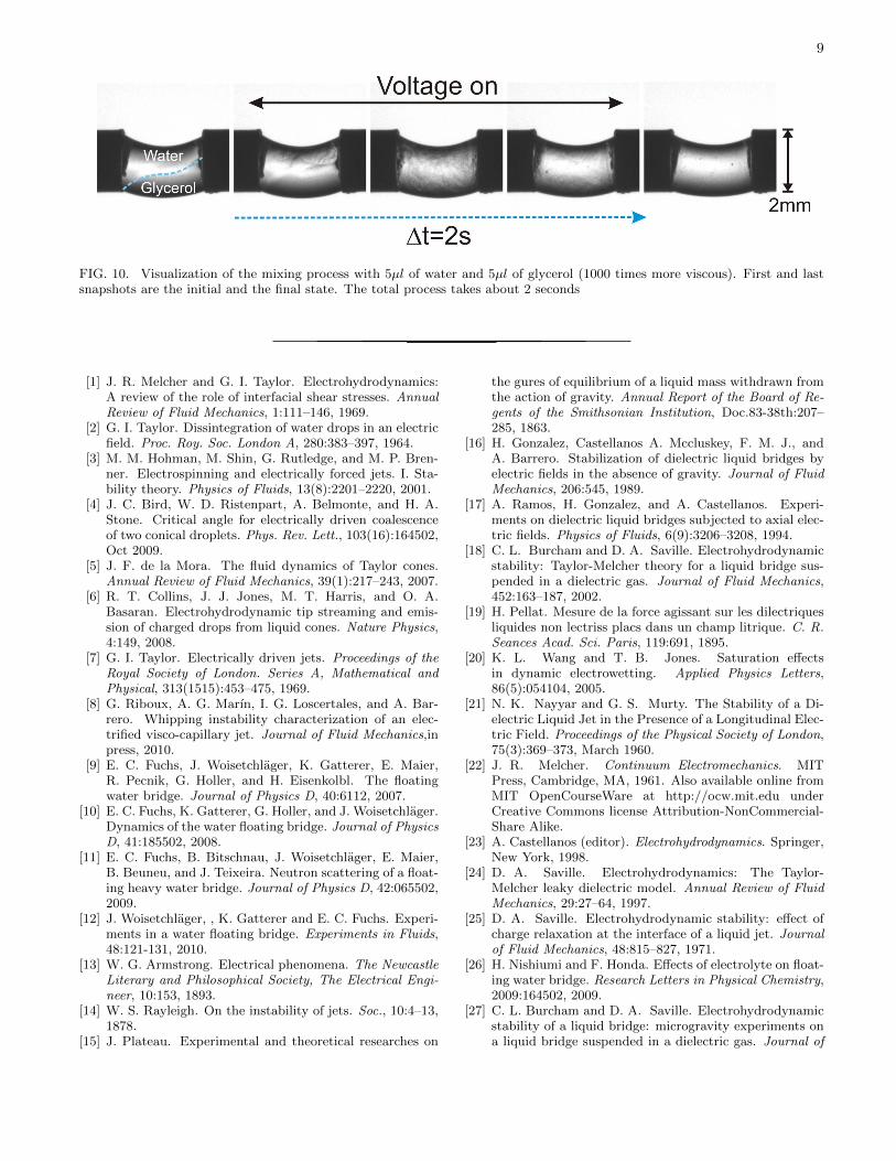
Interestingly enough, this result shows us that highvelocities of order of several millimeters per second orhigher could be reached in bridges of water-based liquidswith small volumes of a few microliters. Such a featurecould have great benefits for efficiently mixing of smallvolumes of liquids. In the following experiment, a 5 mi-croliter droplet of deionized water is placed at the exitof one cylinder and 5 microliter droplet of pure glycerin(1000 times more viscous than water) in the opposite,when both establish contact, the glycerine phase staysat the bottom and water above (left image in figure 10).Although both liquids are miscible, the difference in vis-cosities and densities makes the mixing of both liquids acomplicated task, impossible to accomplish by diffusionin practical time scales. When the voltage is elevatedto 15kV (CaE ≈ 10) the liquids are set into motion fol-lowing irregular and unsteady flow patterns. As a con-sequence, the liquids are perfectly mixed within a fewseconds. For this application the liquids do not need tobe directly connected to the electrodes, and the electricalcurrent through the bridge therefore can be controlled.

VI. SUMMARY

In conclusion, the floating water bridge remains sta-ble without breaking for big aspect ratios and unbentby gravity due to the effect of the induced polarizationforces at the interface, generating normal stresses thatcounteract not only capillary forces but also gravity. Toour knowledge, such a balance between polarization ef-fects and gravity has never been reported in the literaturewith the only exception of the Pellat effect[19]. Free sur-face charge is responsible for the observed flow, whichcan be especially intense for aqueous solutions, due totheir lower viscosity and their non negligible conductiv-ity. The main difference with previous studies in thefield, as those by Gonzalez et al.[16][17] and Burcham &Saville[18], consists in the presence of a significant freecharge in the system, which remains out of equilibrium.

In spite of the effort of this contribution, the waterbridge deserves further investigation. Improved and moresophisticated experimental configurations should be de-signed to allow for better flow manipulation and mea-surements.

ACKNOWLEDGMENTS

The authors thank Dr. Elmar Fuchs for making themaware of the phenomenon of the floating water bridge.Alvaro G. Marın thanks especially Dr. Pablo Garcıa-Sanchez for long discussions on the subject and alsoProf. Antonio Ramos for his useful comments. AlvaroG. Marın dedicates this paper to the memory of Prof.Antonio Barrero Ripoll.

9

FIG. 10. Visualization of the mixing process with 5µl of water and 5µl of glycerol (1000 times more viscous). First and lastsnapshots are the initial and the final state. The total process takes about 2 seconds

[1] J. R. Melcher and G. I. Taylor. Electrohydrodynamics:A review of the role of interfacial shear stresses. AnnualReview of Fluid Mechanics, 1:111–146, 1969.

[2] G. I. Taylor. Dissintegration of water drops in an electricfield. Proc. Roy. Soc. London A, 280:383–397, 1964.

[3] M. M. Hohman, M. Shin, G. Rutledge, and M. P. Bren-ner. Electrospinning and electrically forced jets. I. Sta-bility theory. Physics of Fluids, 13(8):2201–2220, 2001.

[4] J. C. Bird, W. D. Ristenpart, A. Belmonte, and H. A.Stone. Critical angle for electrically driven coalescenceof two conical droplets. Phys. Rev. Lett., 103(16):164502,Oct 2009.

[5] J. F. de la Mora. The fluid dynamics of Taylor cones.Annual Review of Fluid Mechanics, 39(1):217–243, 2007.

[6] R. T. Collins, J. J. Jones, M. T. Harris, and O. A.Basaran. Electrohydrodynamic tip streaming and emis-sion of charged drops from liquid cones. Nature Physics,4:149, 2008.

[7] G. I. Taylor. Electrically driven jets. Proceedings of theRoyal Society of London. Series A, Mathematical andPhysical, 313(1515):453–475, 1969.

[8] G. Riboux, A. G. Marın, I. G. Loscertales, and A. Bar-rero. Whipping instability characterization of an elec-trified visco-capillary jet. Journal of Fluid Mechanics,inpress, 2010.

[9] E. C. Fuchs, J. Woisetchlager, K. Gatterer, E. Maier,R. Pecnik, G. Holler, and H. Eisenkolbl. The floatingwater bridge. Journal of Physics D, 40:6112, 2007.

[10] E. C. Fuchs, K. Gatterer, G. Holler, and J. Woisetchlager.Dynamics of the water floating bridge. Journal of PhysicsD, 41:185502, 2008.

[11] E. C. Fuchs, B. Bitschnau, J. Woisetchlager, E. Maier,B. Beuneu, and J. Teixeira. Neutron scattering of a float-ing heavy water bridge. Journal of Physics D, 42:065502,2009.

[12] J. Woisetchlager, , K. Gatterer and E. C. Fuchs. Experi-ments in a water floating bridge. Experiments in Fluids,48:121-131, 2010.

[13] W. G. Armstrong. Electrical phenomena. The NewcastleLiterary and Philosophical Society, The Electrical Engi-neer, 10:153, 1893.

[14] W. S. Rayleigh. On the instability of jets. Soc., 10:4–13,1878.

[15] J. Plateau. Experimental and theoretical researches on

the gures of equilibrium of a liquid mass withdrawn fromthe action of gravity. Annual Report of the Board of Re-gents of the Smithsonian Institution, Doc.83-38th:207–285, 1863.

[16] H. Gonzalez, Castellanos A. Mccluskey, F. M. J., andA. Barrero. Stabilization of dielectric liquid bridges byelectric fields in the absence of gravity. Journal of FluidMechanics, 206:545, 1989.

[17] A. Ramos, H. Gonzalez, and A. Castellanos. Experi-ments on dielectric liquid bridges subjected to axial elec-tric fields. Physics of Fluids, 6(9):3206–3208, 1994.

[18] C. L. Burcham and D. A. Saville. Electrohydrodynamicstability: Taylor-Melcher theory for a liquid bridge sus-pended in a dielectric gas. Journal of Fluid Mechanics,452:163–187, 2002.

[19] H. Pellat. Mesure de la force agissant sur les dilectriquesliquides non lectriss placs dans un champ litrique. C. R.Seances Acad. Sci. Paris, 119:691, 1895.

[20] K. L. Wang and T. B. Jones. Saturation effectsin dynamic electrowetting. Applied Physics Letters,86(5):054104, 2005.

[21] N. K. Nayyar and G. S. Murty. The Stability of a Di-electric Liquid Jet in the Presence of a Longitudinal Elec-tric Field. Proceedings of the Physical Society of London,75(3):369–373, March 1960.

[22] J. R. Melcher. Continuum Electromechanics. MITPress, Cambridge, MA, 1961. Also available online fromMIT OpenCourseWare at http://ocw.mit.edu underCreative Commons license Attribution-NonCommercial-Share Alike.

[23] A. Castellanos (editor). Electrohydrodynamics. Springer,New York, 1998.

[24] D. A. Saville. Electrohydrodynamics: The Taylor-Melcher leaky dielectric model. Annual Review of FluidMechanics, 29:27–64, 1997.

[25] D. A. Saville. Electrohydrodynamic stability: effect ofcharge relaxation at the interface of a liquid jet. Journalof Fluid Mechanics, 48:815–827, 1971.

[26] H. Nishiumi and F. Honda. Effects of electrolyte on float-ing water bridge. Research Letters in Physical Chemistry,2009:164502, 2009.

[27] C. L. Burcham and D. A. Saville. Electrohydrodynamicstability of a liquid bridge: microgravity experiments ona liquid bridge suspended in a dielectric gas. Journal of

10

Fluid Mechanics, 405:37–56, 2000.[28] S. Tomotika. On the instability of a cylindrical thread

of a viscous liquid surrounded by another viscous fluid.Proc. Roy. Soc. London A, 150, 1935.

[29] D. A. Saville. Electrohydrodynamic Stability - FluidCylinders In Longitudinal Electric Fields. Physics OfFluids, 13(12):2987–&, 1970.

[30] J. R. Melcher and E. P. Warren. Electrohydrodynamicsof a current-carrying semi-insulating jet. Journal of FluidMechanics, 47:127–143, 1971.

[31] A. Widom, J. Swain, J. Silverberg, S. Sivasubramanian,and Y. N. Srivastava. Theory of the Maxwell pressure

tensor and the tension in a water bridge. Physical ReviewE, 80:016301, 2009.

[32] A. G. Marın, I. G. Loscertales, and A. Barrero. Coni-cal tips inside cone-jet electrosprays. Physics of Fluids,20(4):042102, 2008.

[33] O. A. Basaran and L. E. Scriven. The Taylorpump: viscous-free surface flow driven by electric shear-stress. Chemical Engineering Communications, 67:259–273, 1988.

[34] T. B. Jones An electromechanical interpretation of elec-trowetting. Journal Of Micromechanics And Microengi-neering,15:6, 2005.