Building Qualitative Modelsof Thermodynamic Processes

John W . CollinsKenneth D . Forbus

Qualitative Reasoning GroupBeckman Institute, University of Illinois

405 North Mathews St.Urbana, IL 61801

Abstract

This paper describes a qualitative domain theory for core phenomena in engineeringthermodynamics, expressed in Qualitative Process theory . It represents many of thebest features of domain models developed by our group over the past five years . Itfocuses on supporting system-level qualitative analyses of typical fluid and thermalsystems, such as refrigerators and power plants . We use explicit modeling assumptions[3] to control the level of detail used in building models of specific scenarios. We beginby outlining the primitives of the specific QP modeling language . The bulk of the paperdescribes the domain model itself, highlighting our design choices, simplifications, anduse of modeling assumptions . Next we demonstrate how this domain model can beused to build models of a variety of specific scenarios, including simplified versions ofa refrigerator, a steam plant, and a thermal control system . Finally, we describe someplanned extensions to the model .

Contents

1 Introduction

4

2 Modeling Issues

5

3 An Overview of the QPE Modeling Language

73 .1 Defining objects, properties, and relationships 7

3 .2 Qualitative Mathematics 8

3 .3 Defining views and processes 9

3 .4 Defining perspectives 10

4 A Tour of the Core Thermodynamics Model

114 .1 The Organization of the Model 11

4 .2 Types of Objects 12

4.2 .1 Physical Objects 12

4.2 .2 Containers 15

4.2 .3 Contained Stuffs 18

4.2 .4 Paths, Portals and Connectivity 24

4 .3 Flow Processes 36

4.3 .1 Heat Flow 36

4.3 .2 Fluid Flow 38

4.3 .3 Thermal Effects of Fluid Flow 41

4.3 .4 Pumped Flow 42

4 .4 Phase Transition Processes 47

4.4 .1 Thermal Behavior of Phase Transitions 48

4.4 .2 Core of the Boiling Model 50

4.4 .3 Condensation 53

4 .5 Controlling the Model 56

4.5 .1 Representing and enforcing the steady-state assumption 56

4.5 .2 Representing Nominal Values 56

4.5 .3 Enforcing Relationships Between Modeling Assumptions 57

5 Examples

595 .1 Modeling a Simple Fluid Flow System 61

5 .2 Modeling a Pumped Flow System 64

5 .3 Modeling a Thermal Control System 66

5 .4 Modeling a Refrigerator 66

5 .5 Modeling a shipboard propulsion plant 70

5 .6 Summary of Examples 70

6 Discussion

72

7 Acknowledgements

74

1

List of Figures

1

Defining quantities associated with physob 13

2

Defining quantities associated with physob 14

3

Definition for Container 15

4

Definition for Geometric-Container 17

5

Definition for Contained-Stuff 19

6

Definition of Contained-Liquid 20

7

Novel environmental conditions can be handled compositionally 21

8

Definition of Contained-Gas 22

9

Definition of single-substance phase mixtures 24

10

Definition of single-substance mixtures, continued 25

11

Definition for Fluid–Paths 27

12

Defining connections 27

13

Establishing possible path contents without portals 28

14

Direct implications of connectivity 28

15

Selecting which pressure to use in inferring flow 29

16

Definition of heat paths 30

17

Valve definition 30

18

Valve status 31

19

Valve dynamics 32

20

Portals detail how paths connect to containers 32

21

Properties of portals 33

22

Describing what touches a portal 33

23

Relating pressures of portals in the same container 34

24

Relating pressures of portals which share a common path 35

25

Process Definition for Heat Flow 36

26

Modifications to heat flow 37

27

Process definition for fluid flow 39

28

Modifying flow rates according to conductance assumptions 40

29

Transfer of heat during fluid flow 40

30

Thermal mixing due to fluid flow 41

31

Types of pumps 43

32

Expressing pump connectivity 43

33

Two models of pump flow rates 44

34

Representing pump priming 45

35

A model of pumped flow 46

36

Different states of pumps 46

37

Establishing when boiling can occur 51

38

Core of boiling process 51

39

Defining the rate of the boiling process 52

40

Thermal effects of boiling 53

41

Establishing when condensing might occur 54

2

42 Condensation process 54

43 Rate of condensation 55

44 Heat flow in condensation 55

45 The logic of steady-state 56

46 Representing tolerances 57

47 Inheriting modeling assumptions 58

48 Perspectives for controlling modeling assumptions 59

49 ATMoSphere rules for modeling assumption consequences 60

50 Typical settings for modeling assumptions 60

51 A path connecting two containers 61

52 Scenario input for a path between two containers 61

53 Envisionment for simple flow with thermal properties 62

54 Envisionment for simple flow without thermal properties 63

55 A pump and a path connecting two containers 64

56 Scenario input for a pump and a return path between two containers . .

64

57 Envisionment for the Pump Cycle example (without thermal properties)

65

58 High-level sketch of Thermal Control System design 67

59 Scenario Description for TCS LOOP A : 68

60 A two-phase refrigeration system 68

61 Scenario description for the refrigerator 69

62 A simplified shipboard propulsion plant 71

63 Scenario description for simplified propulsion plant 71

3

1 Introduction

This paper develops a qualitative domain model for thermodynamic and fluid systems,based on Qualitative Process theory . This model incorporates many of the best features ofthe domain models our group has been developing over the last five years . Several domainmodels for such systems have been described previously [5,3], but have various limitations.

The FSThermol domain model exhibits three important features:

• Broad Coverage : Previous models (e .g., [5]) covered only a small subset of relevantphenomena. The FSThermo model captures a broader spectrum of phenomena. Forexample, it defines richer models for a variety of physical processes, including fluidflows (liquid or gas, forced or free), heat flows, and phase transitions between theliquid and gaseous phases.

• Fine Grain: The FSThermo model provides more detailed perspectives of severalphenomena, such as the role of portals in fluid systems and latent heat in boiling,than previous qualitative models.

• Modeling Assumptions : The domain model of [3] demonstrated that modeling as-sumptions could be used to organize abstract, system-specific models . Here we usethe same methodology to control a fine-grained model, showing that by varying thegranularity appropriately, a quite intricate qualitative domain theory can still beefficiently used to answer questions.

Furthermore, this is the first detailed description of the design choices underlying asubstantial domain model . We have tried to be explicit about our reasons for variousdesign choices, and where our simplifying assumptions impact the model, for good or ill.While this is not a tutorial for QP modeling, we hope it will be useful to other qualitativemodelers. We also show how the FSThermo model can be used to model a variety ofsystems, including a steam plant, refrigerator, and a thermal control system for NASA'sspace station.

Section 2 begins by outlining some issues involved in building domain models . Next,Section 3 describes the modeling language we use . Specifically, the domain model is writtenin the language of QPE[8], an envisioner for Qualitative Process theory . We assume a readingknowledge of QP theory : This section only describes some of the implementation-specificproperties of this modeling language that are important in understanding how the domainmodel is used . Section 4 describes the FSThermo model itself . We begin with basic objectand structural descriptions and examine how flows are modeled . We describe phase changesand pumps next . Finally, we examine the interrelationships between the various modelingassumptions and the encoding and importance of the steady-state assumption . Section 5shows a variety of systems modeled using FSThermo . We show how the same structuraldescription can lead to a variety of models, according to what simplifying assumptionsare in force, and analyze the consequences for the complexity of qualitative simulation.

'FSThermo stands for Fine Structure THERMOdynamics.

4

We also see how models of larger (although still abstract) systems can be successfullysimulated in minutes yielding a handful of states, rather than days and thousands ofstates, if performing reasonable analyses . Finally, Section 6 outlines what we have learnedby building this model, and makes suggestions concerning future domain models, modelinglanguages, and qualitative reasoners.

2 Modeling Issues

An important feature of Qualitative Process theory is that it makes more of the modelingprocess explicit . That is, knowledge of the physical world is organized as a domain model,which describes the basic conceptual entities and phenomena . Given a particular physicalsituation, constructs of the domain model are combined to form a scenario model of thespecific situation.

Component-centered ontologies [2,16] are also organized in this way, but subject tothe following restrictions . First, it is assumed that all primitive phenomena can always beassociated with a single, explicit component . Second, the interactions between componentsare in terms of shared quantities only, and do not involve the introduction of new objects.Finally, the process of mapping from a structural description to elements of the componentlibrary is assumed to be straightforward (or at least left outside the scope of existingtheories) . While these restrictions work reasonably well for electronics, they do not workvery well for most engineering domains (e .g., thermodynamics), and quite poorly for manyimportant domains (e .g ., motion).

A process-centered ontology is more apt for thermodynamics and fluid systems . Manythermodynamic phenomena are typically conceptualized as processes. Furthermore, fluidsystems have non-trivial node capacities, so the approximation represented by Kirchoff'sCurrent Law is often inappropriate . The mapping from a structural description to con-ceptual entities is also more complex in fluid and thermal problems . For example, in someproblems the geometry of containers is important, and in others it is not . (This is actu-ally true for electronics as well, outside the usual (implicit) assumptions of low-frequencysignals .) The need for multiple levels of granularity cannot be ignored in engineeringthermodynamics problems.

QP theory also provides an additional source of leverage, beyond its ability to expressprocess-centered models . It provides ways to encode explicit modeling assumptions, sothat the problem of building a model for a specific scenario from a domain model becomesa subject for explicit reasoning by the QP interpreter . Developing a domain model that iscapable of covering a wide variety of fluid and thermodynamic phenomena requires carefulconsideration of several issues:

Composability Anticipating every potential scenario is impossible . Instead, the con-structs of the domain model are composable . That is, complex systems and behaviors canbe described by applying and combining the results of many simple, local descriptions.Furthermore, we attempt to minimize the number of primitive constructs . It would be a

5

mistake, for example, to encode the activity in the normal, steady-state operating modeof a steam plant as a single process . This model would apply in very few situations, andcommon phenomena with similar systems would remain implicit . Instead, we limit our-selves to describing only fundamental physical processes in the domain model . Of course,an engineer's stock of knowledge includes detailed information about specific scenarios andclasses of systems (e .g ., two–phase refrigeration systems) . We exclude such specific entriesfrom this domain model . By covering the basic physical phenomena, we hope to providethe constructs needed to ground these more specific models.

Level of Detail A primary modeling decision concerns choosing the appropriate levelof detail . An early step in developing a model for some domain is to partition the domainup into discrete objects . The coarseness of the partitioning determines the coarseness (andefficiency) of the reasoning . For example, reasoning at the level of contained-liquids wouldbe too coarse if our goal were to understand sloshing.

The appropriate level of detail depends on the goals of the modeler . For instance,the desired level of performance (expert or novice) greatly influences modeling choices.Likewise, a model for only examining nominal operations will look very different from amodel designed to anticipate possible failure modes.

Modeling Idealizations Every finite model only considers those aspects of objects andtheir behaviors deemed relevant by the model–builder . Modeling idealizations ignore as-pects of the model which are either (a) insignificantly small in magnitude, duration, orlikelihood ; (b) outside of the intended functionality for some component ; or (c) qualita-tively uninteresting.

Often we are interested in modeling the long–term or steady–state aspects of a ther-modynamic system, and so choose to ignore transient behaviors . For example, our modelfor fluid flow ignores the acceleration of the fluid in the path, in favor of an equilibriummodel which relates flow rate and pressures directly.

A quantity which never changes might be viewed as qualitatively uninteresting . Forexample, the conductance (or resistance) of a fluid path is generally constant, and can beexcluded from the model by defining the flow rate as the qualitative difference in pressuresacross the path . However, having conductance provides a hook for adding a continuousmodel for valves (Section 4 .2.4), and avoids the direct comparison of quantities of differentunits (eg . flow-rate and pressure).

Modeling Assumptions As models develop, many choices must be made between dis-tinct perspectives on phenomena and different levels of detail . When multiple alternativeslook useful, one might split the model into seperate pieces . But as the number of optionsgrows, the number of distinct models can rise exponentially . By organizing domain modelsaround modeling assumptions, conflicting models can peacefully co-exist.

Here modeling assumptions typically take the form (Consider ?X), where ?X repre-sents some aspect or dimension which is or is not being included in the scenario modelunder construction .

6

Modularity To manage complexity, the domain model is partitioned into a set of rel-atively independent modules . For example, heat flow is sufficiently different from otherprocesses in thermodynamics to be considered a separate module . No module is totallyindependent from the others ; heat flows involve physical objects, as do all other processes.In general each module depends on a set of lower modules, and may be used by still highermodules.

As a matter of pragmatics, each module is stored in a separate file . This allows anevolving model to be compiled incrementally ; in addition, only those modules required fora particular scenario need be loaded.

Not surprisingly, hierarchical representation is useful in qualitative physics . Hierarchiesare used extensively in representing physical entities ; for example, a contained—liquid isa contained—stuff, which is a physob (physical object) . Quantities and other propertiesare inherited from the general class to the specific instance. Hierarchical representationshave also been applied to processes, though to a lesser extent . For example, there is muchin common between liquid flow and gas flow . Consequently, we have defined a common,abstract fluid-f low process to contain their intersection, and ancillary perspectives whichrepresent phase-specific details . No new, special syntax is introduced to handle hierarchies— we simply use logical implication and the binding abilities of normal QP descriptions.

3 An Overview of the QPE Modeling Language

Our representations are encoded in QP theory. The syntax is that used by the modelinglanguage associated with a particular program which implements QP theory, called QPE.

Given a domain model, a structural description, and a collection (possibly empty) ofmodeling assumptions, QPE constructs a model of that scenario based on the constructsof the domain model, and produces a total envisionment of it . The details of how QPE

works are described in [8] . This modeling language is quite close to the syntax used inthe original QP papers, but has the advantage that it is executable . Almost no specialproperties of this modeling language are essential to understanding the domain model, butwe point out any interactions below.

3 .1 Defining objects, properties, and relationships

The form Defquantity-type introduces a new kind of quantity . The first argument is thename of the type of quantity. Each quantity type is considered a function, and the rest ofthe arguments are the arguments of that function . Each argument is declared as either anindividual or a constant . This information is used in computing whether or not a quantityexists in a particular situation . That is, if any of the individuals the quantity is associatedwith do not exist, then that quantity does not exist . For example, if we were describingthe temperature of the arsenic in a cup of coffee, and there was no arsenic, then it wouldbe meaningless to talk about its temperature.

An example of Def Quantity-Type is

(defQuantity-Type distance individual individual)

7

which allows us to describe distances between two entities, such as

(greater-than (A (distance Urbana Chicago)) (A (distance Evanston Chicago)))

QPE 's vocabulary now includes defPredicate, which may be used to specify conse-quences of a single antecedent predicate . The first argument to defpredicate is thepredicate whose consequences are being defined. The rest is the body, which constitutesa set of consequences which should be believed when the predicate is believed . When thepredicate is a single symbol, then it is implicitly a unary predicate, with the variable ?self

bound to the object of the predicate . defEntity is similar, but also implies existence ofits object.

For example, we might define some of the economic aspects of a person by

(defEntity Person(Quantity (income ?self))(Quantity (net-worth ?self)))

which indicates that when a person exists, they have some income and net worth . (Tobe less dismal we might constrain these quantities to be non-negative .) Then to definesomeone as solvent for some purpose, we might say

(defPredicate (Solvent-For ?person ?purpose)(greater-than (A (net-worth ?person)) (A (cost-of ?purpose))))

that is, their net worth is more than the cost of the thing they want to do.

3 .2 Qualitative MathematicsThe standard modeling primitives of QP theory are available, albeit in a lisp-style syntax.That is, where in theoretical papers one might see

Q1 ° Q+ Q2Q1 o(Q— Q3

we will write

(QProP + Q 1 Q2)(Qprop- Q1 Q3)

Other primitives are translated to lisp-style syntax in the obvious fashion . Severalnew primitives are special versions of existing ones which exploit computational sav-ings available for special cases . For instance, an Ordered-Correspondence is a form ofCorrespondence which assumes a positive qualitative proportionality ; this permits QPE touse a simpler set of internal justifications to enforce its semantics . Similarly, *0+ and /0+are special versions of multiplication and division which assume that their arguments arenon-negative.

There are two other important things to note about the algebraic primitives used inQPE . First, qualitative proportionalities and direct influences have a causal interpretationas well as a mathematical one . That is,

(Qprop+ (temperature ?obj) (heat ?obj))

8

indicates that a change in heat (i .e., internal energy) causes a change in temperature, aswell as indicating that when the heat rises the temperature will, all else being equal . Inthe case of direct influences, the process in which the I+ or I- appears is causing a changein the first parameter, at a rate specified by the second parameter . Thus if the only directinfluence on (heat ?obj) was (flow-rate ?heat-f low) and imposed by an instance ofheat flow, that is,(I+ (heat ?obj) (flow-rate ?heat-flow))

it would indicate both that the instance of the heat flow process was the cause of anychange in (heat ?obj) 2 , and that

(D (heat ?obj)) = (A (flow-rate ?heat-flow))

The second point is that the semantics of +, -, *, and / are defined in terms of qualitativeproportionalities and correspondences .' Thus they inherit the causal interpretation of thequalitative proportionalities they expand into . Thus the expression

(Q= (Temperature ?self) (/0+ (heat ?self) (mass ?self)))

indicates that temperature causally depends on heat and mass, as well as indicating themathematical nature of the relationship.

There is an additional subtlety concerning direct influences . If the quantity beinginfluenced does not exist, the direct influence has no effect . This stipulation greatly sim-plifies defining processes which behave properly when their effects cause objects to comeinto existence . Otherwise, one often needs to double the number of process descriptionsfor certain phenomena, to handle the instant in which a process acts before the stuff itproduces appears.

3 .3 Defining views and processes

The basic syntax of views and processes is a lispified version of the normal QP syntax . Forexample, we might define a budget with a surplus as(defview (surplus ?gov)Individuals ((?gov :type government))QuantityConditions ((greater-than (A (resources ?gov)) zero))Relations ((Probability (during-election-year) High)))

That is, the relationship surplus happens to things which are governments, whentheir resources are greater than zero, and the direct consequence of a surplus is that it isprobably an election year.

Each entry in the individuals field contains a variable and some restrictions on whatit can be bound to . The syntax and meaning of the restrictions are explained below . Byconvention, each entry is thought of as defining a role for each instance of that view (orprocess), hence one can speak of the gov of an instance of surplus as a function mappingfrom view instances to the individual filling that role.

Processes are specified similarly:

'We haven't specified the sign of (flow-rate ?heat-f low) here, remember, so we don't know for a fact

that there is a change.'For products and ratios, these must be conditioned on the signs of the appropriate multipliers/divisors.

9

(defprocess (Taxation ?sap ?gov)Individuals ((?gov type government)

(?sap type personconditions (honest ?sap)))

Relations ((quantity taxes)(greater-than (A taxes) zero)(Qprop- taxes (resources ?gov)))

Influences ((I+ (resources ?gov) (A taxes))(I- (net-worth ?sap) (A taxes))))

Notice that some additional syntax has been added to the individuals field to fa-cilitate more expressive pattern-matching . In particular, it is stipulated that entries inthe individuals field are matched sequentially, in order of appearance . The followingkeywords are supported:

:type Indicates that the next token is a unary predicate which must hold for an instanceto exist.

:form Indicates that the variable can only be bound to expressions which match thepattern which follows.

:bind Indicates that the variable is to be bound to the form which follows . The formmust contain variables, all of which are bound by earlier entries in the individuals

field.

:test Indicates that the next form is a lisp expression which must be non-nil for aninstance to be created with the bindings so far.

: conditions Indicates that all the remaining forms in the entry are additional statementswhich must hold for an instance to be created. Obviously, : conditions must be thelast keyword in any entry.

One should think of :form, :bind, and :test as extra controls on the instantiation ofviews and processes, while : type and : conditions provide the antecedents which justifycreation of an instance . That is, the instance of a view or process exists exactly whenthe union of any statements generated by the bindings of the : type and : conditionsmodifiers hold . Notice that if any of these statements is known to be false such an instancecan never exist, let alone be active . The implementation is guaranteed to respect thisconstraint by never creating instances of views or processes if one of these antecedents isknown to be false at creation time 4 . This stipulation is what allows us to control the levelof detail when instantiating scenario models.

3 .4 Defining perspectives

Sometimes it is useful to exploit the pattern-matching machinery introduced above todefine new predicates which do not have quantity conditions (and hence do not contribute

4A common bug in domain models is that sometimes the falseness of some antecedent isn't discovereduntil after the instance is created . The record of instances of processes and views are never erased, eventhough their existence is carefully predicated on the appropriate antecedents.

10

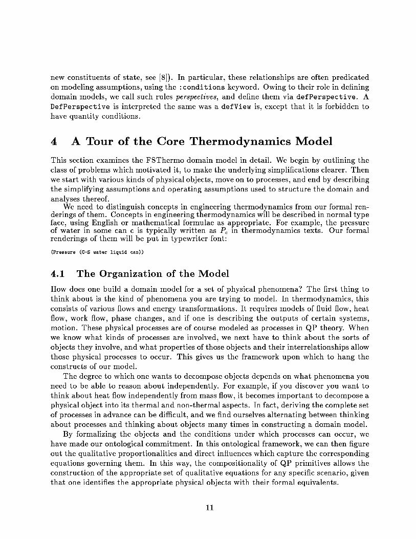
new constituents of state, see [8]) . In particular, these relationships are often predicated

on modeling assumptions, using the : conditions keyword. Owing to their role in defining

domain models, we call such rules perspectives, and define them via defPerspective. A

DefPerspective is interpreted the same was a def View is, except that it is forbidden to

have quantity conditions.

4 A Tour of the Core Thermodynamics Model

This section examines the FSThermo domain model in detail . We begin by outlining the

class of problems which motivated it, to make the underlying simplifications clearer . Then

we start with various kinds of physical objects, move on to processes, and end by describing

the simplifying assumptions and operating assumptions used to structure the domain and

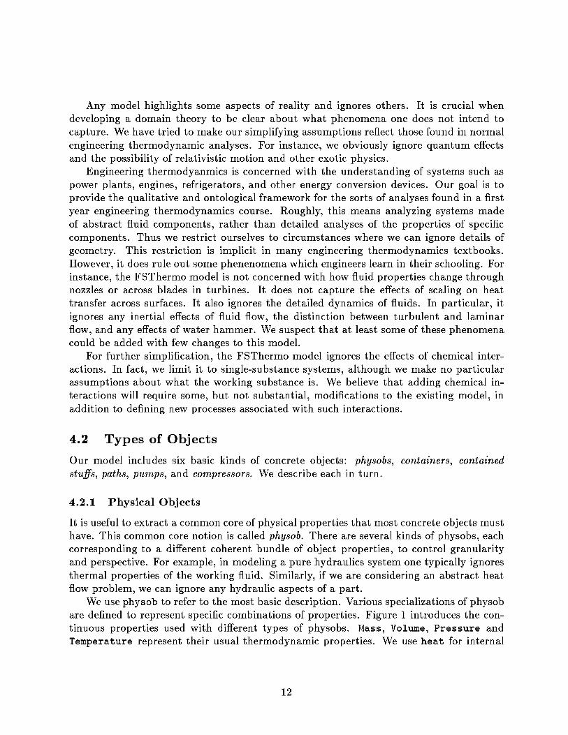
analyses thereof.We need to distinguish concepts in engineering thermodynamics from our formal ren-

derings of them . Concepts in engineering thermodynamics will be described in normal typeface, using English or mathematical formulae as appropriate . For example, the pressureof water in some can c is typically written as Pe in thermodynamics texts . Our formalrenderings of them will be put in typewriter font:

(Pressure (C-S water liquid can))

4 .1 The Organization of the Model

How does one build a domain model for a set of physical phenomena? The first thing to

think about is the kind of phenomena you are trying to model . In thermodynamics, this

consists of various flows and energy transformations . It requires models of fluid flow, heat

flow, work flow, phase changes, and if one is describing the outputs of certain systems,

motion . These physical processes are of course modeled as processes in QP theory . When

we know what kinds of processes are involved, we next have to think about the sorts of

objects they involve, and what properties of those objects and their interrelationships allow

those physical processes to occur . This gives us the framework upon which to hang the

constructs of our model.

The degree to which one wants to decompose objects depends on what phenomena you

need to be able to reason about independently. For example, if you discover you want to

think about heat flow independently from mass flow, it becomes important to decompose a

physical object into its thermal and non-thermal aspects . In fact, deriving the complete set

of processes in advance can be difficult, and we find ourselves alternating between thinking

about processes and thinking about objects many times in constructing a domain model.

By formalizing the objects and the conditions under which processes can occur, we

have made our ontological commitment . In this ontological framework, we can then figure

out the qualitative proportionalities and direct influences which capture the corresponding

equations governing them. In this way, the compositionality of QP primitives allows the

construction of the appropriate set of qualitative equations for any specific scenario, given

that one identifies the appropriate physical objects with their formal equivalents.

11

Any model highlights some aspects of reality and ignores others . It is crucial whendeveloping a domain theory to be clear about what phenomena one does not intend tocapture. We have tried to make our simplifying assumptions reflect those found in normalengineering thermodynamic analyses . For instance, we obviously ignore quantum effectsand the possibility of relativistic motion and other exotic physics.

Engineering thermodyanmics is concerned with the understanding of systems such aspower plants, engines, refrigerators, and other energy conversion devices . Our goal is toprovide the qualitative and ontological framework for the sorts of analyses found in a firstyear engineering thermodynamics course . Roughly, this means analyzing systems madeof abstract fluid components, rather than detailed analyses of the properties of specificcomponents . Thus we restrict ourselves to circumstances where we can ignore details ofgeometry. This restriction is implicit in many engineering thermodynamics textbooks.However, it does rule out some phenenomena which engineers learn in their schooling . Forinstance, the FSThermo model is not concerned with how fluid properties change throughnozzles or across blades in turbines . It does not capture the effects of scaling on heattransfer across surfaces . It also ignores the detailed dynamics of fluids . In particular, itignores any inertial effects of fluid flow, the distinction between turbulent and laminarflow, and any effects of water hammer . We suspect that at least some of these phenomenacould be added with few changes to this model.

For further simplification, the FSThermo model ignores the effects of chemical inter-actions . In fact, we limit it to single-substance systems, although we make no particularassumptions about what the working substance is . We believe that adding chemical in-teractions will require some, but not substantial, modifications to the existing model, inaddition to defining new processes associated with such interactions.

4 .2 Types of Objects

Our model includes six basic kinds of concrete objects : physobs, containers, containedstuffs, paths, pumps, and compressors . We describe each in turn.

4 .2 .1 Physical Objects

It is useful to extract a common core of physical properties that most concrete objects musthave . This common core notion is called physob . There are several kinds of physobs, eachcorresponding to a different coherent bundle of object properties, to control granularityand perspective. For example, in modeling a pure hydraulics system one typically ignoresthermal properties of the working fluid . Similarly, if we are considering an abstract heatflow problem, we can ignore any hydraulic aspects of a part.

We use physob to refer to the most basic description . Various specializations of physobare defined to represent specific combinations of properties . Figure 1 introduces the con-tinuous properties used with different types of physobs . Mass, Volume, Pressure andTemperature represent their usual thermodynamic properties . We use heat for internal

12

Figure 1 : Defining quantities associated with physob

Extensive properties(defQuantity-Type Mass Individual)(defQuantity-Type Heat Individual)(defQuantity-Type Volume Individual)

Intensive properties(defQuantity-Type Pressure Individual Individual)(defQuantity-Type Temperature Individual Individual)

(defpredicate non-negative-quantity(quantity ?self)(not (less-than (A ?self) ZERO)))

(defpredicate positive-quantity(quantity ?self)(greater-than (A ?self) ZERO))

energy out of respect for the intuitive language often still found in modern thermodynamictextbooks.

The extensive properties (i .e ., Mass, Heat, and Volume) belong to specific individuals.The intensive properties (i .e ., Pressure and Temperature) are point properties, and henceinvolve a comparison with respect to some frame of reference . We have chosen to makethis comparison explicit in this model . We thus avoid introducing new types of quantitiesto represent OP's and OT's, at the cost of always naming an explicit comparison point.The token : ABSOLUTE is considered to be an abstract individual which always exists andindicates that the comparison is with the appropriate ground or absolute zero value forthat type of quantity 5 .

Figure 1 also defines predicates for sign constraints . Such constraints abound in thermo-dynamics texts, and they are just as crucial in qualitative reasoning . Two specializations ofQuantity are defined using defPredicate : Positive-Quantity ensures that it is alwayslarger than zero, and Non-Negative-Quantity ensures that it is never less than zero.

The actual definitions of physobs is contained in Figure 2 . The first def entity is thebasic notion of physob, which serves as a uniform basis for matching . Thermal propertiesare captured via Simple-Thermal-Physob and Thermal-Physob. A Simple-Thermal-Physob

has Temperature, and a Thermal-Physob is a Simple-Thermal-Physob with Heat . (Thereason for the distinction will become clear in Section 4 .3 .1 .) The temperature of aThermal-Physob is qualitatively proportional to its heat . Thus if the heat of a Thermal-Physob

is influenced (up or down), then its temperature is indirectly influenced in the same direc-tion .

A Volumetric-Physob has mass and volume. While we know it has these proper-ties, until we know its phase we cannot say anything about how they are related . A

Complex-Physob is both a Thermal-Physob and a Volumetric-Physob . Having both

5Notice that zero pressure here is zero in absolute pressure rather than gauge pressure.

13

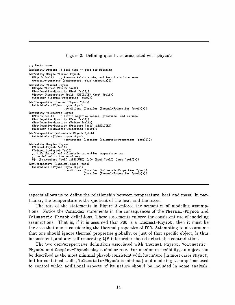
Figure 2 : Defining quantities associated with physob

,, ; Basic types

(defentity Physob) ; ; root type -- good for matching

(defentity Simple-Thermal-Physob(Physob ?self)

; Presume Kelvin scale, and forbid absolute zero.(Positive-Quantity (Temperature ?self :ABSOLUTE)))

(defentity Thermal-Physob(Simple-Thermal-Physob ?self)(Non-Negative-Quantity (Heat ?self))(Qprop+ (temperature ?self :ABSOLUTE) (heat ?self))(Consider (Thermal-Properties ?self)))

(defPerspective (Thermal-Physob ?phob)Individuals ((?phob type physob

conditions (Consider (Thermal-Properties ?phob)))))

(defentity Volumetric-Physob(Physob ?self)

; Forbid negative masses, pressures, and volumes(Non-Negative-Quantity (Mass ?self))(Non-Negative-Quantity (Volume ?self))(Non-Negative-Quantity (Pressure ?self :ABSOLUTE))(Consider (Volumetric-Properties ?self)))

(defPerspective (Volumetric-Physob ?phob)Individuals ((?phob type physob

conditions (Consider (Volumetric-Properties ?phob)))))

(defentity Complex-Physob(Thermal-Physob ?self)(Volumetric-Physob ?self)

With thermal and volumetric properties temperature canbe defined in the usual way:

(Q= (Temperature ?self :ABSOLUTE) (/0+ (heat ?self) (mass ?self))))

(defPerspective (Complex-Physob ?phob)Individuals ((?phob :type physob

conditions (Consider (Volumetric-Properties ?phob))(Consider (Thermal-Properties ?phob)))))

aspects allows us to define the relationship between temperature, heat and mass . In par-ticular, the temperature is the quotient of the heat and the mass.

The rest of the statements in Figure 2 enforce the semantics of modeling assump-tions. Notice the Consider statements in the consequences of the Thermal-Physob andVolumetric-Physob definitions . These statements enforce the consistent use of modelingassumptions . That is, if it is assumed that FOO is a Thermal-Physob, then it must bethe case that one is considering the thermal properties of FOO . Attempting to also assumethat one should ignore thermal properties globally, or just of that specific object, is thusinconsistent, and any self-respecting QP interpreter should detect this contradiction.

The two defPerspective definitions associated with Thermal-Physob, Volumetric-

Physob, and Complex-Physob play a similar role . For maximum flexibility, an object canbe described as the most minimal physob consistent with its nature (in most cases Physob,

but for contained stuffs, Volumetric-Physob is minimal) and modeling assumptions usedto control which additional aspects of its nature should be included in some analysis.

14

Figure 3 : Definition for Container

(defentity Container(Physob ?self)(Positive-Quantity (volume ?self))(Non-Negative-Quantity (volume (liquid-in ?self)))(Non-Negative-Quantity (pressure (gas-in ?self) :ABSOLUTE))(Non-Negative-Quantity (pressure (bottom ?self) :ABSOLUTE))(Qprop+ (pressure (bottom ?self) :ABSOLUTE) (pressure (gas-in ?self) :ABSOLUTE)))

These perspectives provide this service by supporting the appropriate predication if the

corresponding antecedents hold.

This combination of perspectives and consider assumptions appears repeatedly in the

domain model, so we will not dwell on it when it appears again . At first glance it might

appear that the use of Consider assumptions in defEntity descriptions is a violation

of modularity. After all, we are placing what is essentially control information into a

description of a physical object . But this is actually an important feature . The whole

purpose of developing a qualitative language for physical modeling is to be able to encode

information in ways that allows it to be used in reasoning . A language which did not

capture modeling assumptions must perforce leave them implicit, and thus will fail to take

on some of the burden that a qualitative physics must.

4 .2 .2 Containers

Most thermodynamic systems involve fluids existing inside some kind of container . Exam-

ples of objects modeled by containers are evaporators, boilers, and tanks . We are using

the contained stuff ontology for fluids [10,5], so containers play a central role in defining

stuffs.

Containers are defined as specializations of physob . Since volume is a key property of

containers, it is tempting to model containers as volumetric-physobs . However, for the

problems we are considering containers remain in fixed positions . This means we can ignore

their mass, and hence the volumetric-physob description contains excess committments.

Instead, we declare the container to have volume explicitly.

It is worth dwelling on this choice a bit further, since it illustrates an important principle

in building domain models . We are not assuming that genuine physical containers per se

do not have mass . Instead, when we view an object as a container, we are only interested

in those aspects which are relevant to its capacity to contain fluids . If we wish to reason

about moving a pot of water to the stove, we must view the pot both as a container and

as a moveable object, which makes its mass relevant. Similarly, if we wanted to model

containers melting, we could describe the container as a thermal-physob in addition to

describing it as a container. This composability is one of the powerful aspects of the

physics .

15

There are two other crucial choices to be made when modeling containers . One iswhether or not containers are open or closed. This intuitive distinction rests on whetheror not a container is exposed to the atmosphere . Since we can always model an opencontainer by including an explicit fluid path to an entity representing the atmosphere, weassume all containers are closed.

The other choice is how detailed container geometry should be modeled . The detailedthree-dimensional shape of containers is irrelevant for the level analyses we are considering.Essentially, the most detail we need are heights and volumes . However, often we don't evenrequire this much detail . The cost of including container geometry is the introduction of ad-ditional quantities representing geometric properties and additional comparisons betweenthem to express geometric relationships . For some kinds of systems, such as siphons ordevices where gravity head is used to produce flow, this cost is unavoidable . But geometricconsiderations can be ignored for many systems, including most pump-driven ones . Conse-quently we include the modeling assumptions Geometric-Properties to control whetheror not such details are introduced.

Figure 3 shows the basic definition of Container . We assume volumes are alwayspositive : zero-volume "nodes" are not allowed . The main property to represent is pressure,which is important because it determines when material flows are possible. Physically, thepressure in a container depends both on what is in it and where it is measured . If it isfilled with a gas the pressure will be uniform throughout, for example, and if it has bothliquid and gas in it, the pressure at a point will vary with the depth of the liquid coveringit . Expressing these relationships can be quite complex, since they depend on exactly whatexists in a container . When something doesn't exist, neither do its properties 6 . When theamount of a contained stuff shrinks to zero it vanishes, and hence its properties vanish aswell . Maintaining physically correct relationships over such changes in existence can be adaunting task.

Our solution to this problem is to introduce two new abstract individuals : the liquid

in the container and the gas in the container, denoted by the functions liquid-in andgas-in, respectively. These abstract individuals always exist, whether or not there is anyliquid or any gas in the container . When stuff of the appropriate phase exists, these abstractindividuals take on their properties . Otherwise, their properties are constrained to producephysically reasonable results . In particular, we define the volume of the liquid-in, sinceit determines the volume available for any contained gas . Similarly, we define the pressureof the gas-in, because it contributes to the pressure of a liquid.

If portals are used, each portal can have a pressure . If portals are too detailed, weneed some standard measuring point to talk about the pressure of a liquid . We choosethe bottom of the container, allowing us to presume that no matter how little liquid thereis, it will always be in contact with the bottom . (How the connectivity is inferred whenportals are explicit is described in Section 4 .2 .4 .) We assume the function bottom mapsa container to the lowest point of the container's inside . We note the dependence of thebottom pressure on the pressure of the gas-in explicitly with a qualitative proportionality.

'Can one speak seriously of the temperature of the arsenic in the coffee one is drinking and continuedrinking it?

16

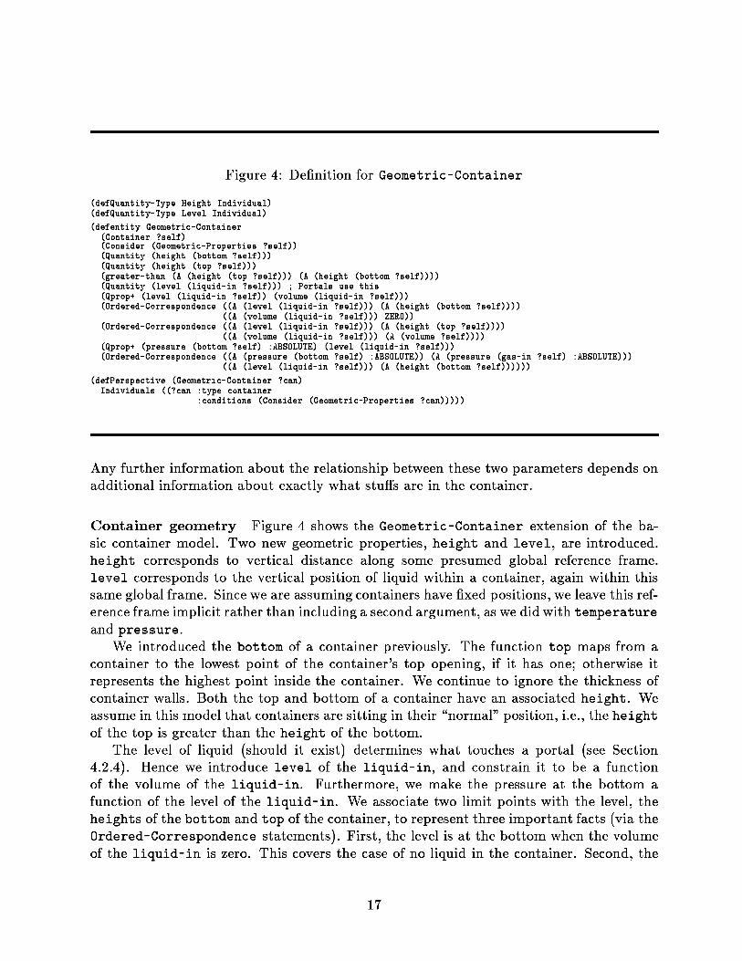
Figure 4 : Definition for Geometric-Container

(defQuantity-Type Height Individual)(defQuantity-Type Level Individual)

(defentity Geometric-Container(Container ?self)(Consider

(Geometric-Properties

?self))(Quantity

(height

(bottom ?self)))(Quantity

(height

(top ?self)))(greater-than

(A

(height

(top ?self)))

(A

(height

(bottom ?self))))(Quantity

(level

(liquid-in ?self)))

; Portals use this(Qprop+

(level

(liquid-in ?self))

(volume

(liquid-in ?self)))(Ordered-Correspondence ((A

((A(level(volume

(liquid-in(liquid-in

?self)))?self)))

(A

(height

(bottom ?self))))ZERO))

(Ordered-Correspondence ((A((A

(level(volume

(liquid-in(liquid-in

?self)))?self)))

(A

(height

(top ?self))))(A

(volume ?self))))(Qprop+ (pressure (bottom ?self) :ABSOLUTE) (level (liquid-in ?self)))(Ordered-Correspondence ((A (pressure (bottom ?self) :ABSOLUTE)) (A (pressure (gas-in ?self) :ABSOLUTE)))

((A (level (liquid-in ?self))) (A (height (bottom ?self))))))

(defPerspective (Geometric-Container ?can)Individuals ((?can :type container

:conditions (Consider (Geometric-Properties ?can)))))

Any further information about the relationship between these two parameters depends onadditional information about exactly what stuffs are in the container.

Container geometry Figure 4 shows the Geometric-Container extension of the ba-sic container model . Two new geometric properties, height and level, are introduced.height corresponds to vertical distance along some presumed global reference frame.level corresponds to the vertical position of liquid within a container, again within thissame global frame. Since we are assuming containers have fixed positions, we leave this ref-erence frame implicit rather than including a second argument, as we did with temperature

and pressure.

We introduced the bottom of a container previously. The function top maps from acontainer to the lowest point of the container's top opening, if it has one ; otherwise itrepresents the highest point inside the container . We continue to ignore the thickness ofcontainer walls . Both the top and bottom of a container have an associated height . Weassume in this model that containers are sitting in their "normal" position, i .e., the height

of the top is greater than the height of the bottom.The level of liquid (should it exist) determines what touches a portal (see Section

4 .2.4) . Hence we introduce level of the liquid-in, and constrain it to be a functionof the volume of the liquid-in . Furthermore, we make the pressure at the bottom afunction of the level of the liquid-in . We associate two limit points with the level, theheights of the bottom and top of the container, to represent three important facts (via theOrdered-Correspondence statements) . First, the level is at the bottom when the volumeof the liquid-in is zero. This covers the case of no liquid in the container . Second, the

17

level is at the top when the volume of the liquid-in is the same as the volume of thecontainer . This helps define fullness and sets the conditions for overflows . Finally, weconstrain the pressure at the bottom to be the pressure of the gas-in when the level is atthe bottom, e.g ., when no liquid is present.

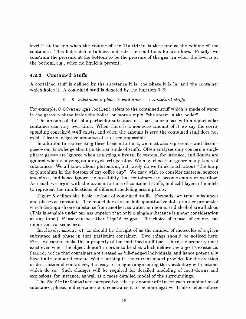
4 .2 .3 Contained Stuffs

A contained stuff is defined by the substance it is, the phase it is in, and the containerwhich holds it . A contained stuff is denoted by the function C-S:

C — S : substance x phase x container —* contained stuffs

For example, C-S (water , gas ,boiler) refers to the contained stuff which is made of waterin the gaseous phase inside the boiler, or more simply, "the steam in the boiler".

The amount of stuff of a particular substance in a particular phase within a particularcontainer can vary over time . When there is a non-zero amount of it we say the corre-sponding contained stuff exists, and when the amount is zero the contained stuff does notexist . Clearly, negative amounts of stuff are impossible.

In addition to representing these basic intuitions, we must also represent — and decom-pose — our knowledge about particular kinds of stuffs . Often analyses only concern a singlephase: gasses are ignored when analyzing a hydraulic system, for instance, and liquids areignored when analyzing an air-cycle refrigerator . We may choose to ignore many kinds ofsubstances : We all know about plutonium, but rarely do we think much about "the lumpof plutonium in the bottom of my coffee cup" . We may wish to consider material sourcesand sinks, and hence ignore the possibility that containers can become empty or overflow.As usual, we begin with the basic intuitions of contained stuffs, and add layers of modelsto represent the ramifications of different modeling assumptions.

Figure 5 defines the basic notions of contained stuffs. Formally, we treat substancesand phases as constants . The model does not include quantitative data or other propertieswhich distinguish one substance from another, so water, ammonia, and alcohol are all alike.(This is sensible under our assumption that only a single substance is under considerationat any time .) Phase can be either liquid or gas. The choice of phase, of course, hasimportant consequences.

Intuitively, amount-of-in should be thought of as the number of molecules of a givensubstance and phase in that particular container . Two things should be noticed here.First, we cannot make this a property of the contained stuff itself, since the property mustexist even when the object doesn't in order to be that which defines the object's existence.Second, notice that containers are treated as full-fledged individuals, and hence potentiallyhave finite temporal extent . While nothing in the current model provides for the creationor destruction of containers, it is easy to imagine augmenting the vocabulary with actionswhich do so. Such changes will be required for detailed modeling of melt-downs andexplosions, for instance, as well as a more detailed model of the surroundings.

The Stuff-In-Container perspective sets up amount-of-in for each combination ofsubstance, phase, and container and constrains it to be non-negative . It also helps enforce

18

Figure 5: Definition for Contained-Stuff

(defQuantity-Type amount-of-in Constant Constant Individual)

(defperspective (stuff-in-container ?s ?st ?c)

Individuals ((?s

type Substance)(?st type Phase

conditions (Consider ?st))

(?c

type Container))Relations ((Non-Negative-Quantity (Amount-of-in ?s ?st ?c))

(when (not (Can-Contain-Substance ?c ?s ?st))(equal-to (A (Amount-of-in ?s ?st ?c)) ZERO))

(when (Can-Contain-Substance ?c ?s ?st)(when (not (Consider (Empty-Container ?c)))(greater-than (A (Amount-of-in ?s ?st ?c)) ZERO)))

(when (Consider Capable-Containers)(Can-Contain-Substance ?c ?s ?st))))

(defview (Contained-Stuff ?cs)Individuals ((?can type container)

(?sub type substance)(?st type phase

conditions (Consider ?st)(Consider Changing-Existence))(?cs bind (C-S ?sub ?st ?can)))

Preconditions ((Can-Contain-Substance ?can ?sub ?st))QuantityConditions ((greater-than (A (amount-of-in ?sub ?st ?can)) ZERO))Relations ((there-is-unique ?cs)))

(defperspective (Contained-Stuff ?cs)Individuals ((?can type container)

(?sub type substance)(?st type phase

conditions (Consider ?st) (Can-Contain-Substance ?can ?sub ?st)(not (Consider Changing-Existence)))

(?cs bind (C-S ?sub ?st ?can))))

(defentity (contained-stuff (C-S ?sub ?st ?can))(Volumetric-Physob (C-S ?sub ?st ?can))(Q= (mass (C-S ?sub ?st ?can)) (amount-of-in ?sub ?st ?can)))

(defentity (Contained-Stuff (C-S ?sub liquid ?can))(Contained-Liquid (C-S ?sub liquid ?can))(Q= (volume (liquid-in ?can)) (volume (C-S ?sub liquid ?can))))

(defentity (Contained-Stuff (C-S ?sub gas ?can))(Contained-Gas (C-S ?sub gas ?can)))

various properties and modeling assumptions about stuffs . First, we may know that acontainer cannot contain certain kinds of stuffs (e .g ., nitric acid in a copper beaker orsulphuric acid in a paper cup) . Such facts are indicated by the appropriate instance ofCan-Contain-Substance being false, and this perspective pins the amount-of-in in thesecases to be zero . Second, if we want to assume that a container is never empty, then we con-strain the amount-of-in to be positive. Finally, the assumption of Capable-Containersis tantamount to assuming that every container can contain every substance in any phase,which is enforced by justifying Can-Contain-Substance for each combination . (This as-sumption is used to simplify the specification of inital conditions in scenario models . Ifit is false, the scenario modeler must have some external theory which introduces theappropriate instances of Can-Contain-Substance, or do so by hand .)

The Contained-Stuff view defines existence if we are allowing contained stuffs tohave finite temporal extent (as evidenced by the dependence on the Changing-Existence

19

Figure 6 : Definition of Contained-Liquid

(defentity Contained-Liquid(Qprop+ (volume ?self) (mass ?self))(Ordered-Correspondence ((A (volume ?self)) ZERO)

((A (mass ?self)) ZERO)))

(defPerspective (Contained-Liquid-Geometry ?cl)Individuals ((?can type Geometric-Container

conditions (Consider Gravity) (Consider (Geometric-Properties ?can)))(?cl

type Contained-Liquidform (C-S ?sub liquid ?can)))

Relations ((Quantity (level ?cl))(not (less-than (A (level ?cl)) (A (height (bottom ?can)))))(Qprop+ (level ?cl) (volume (liquid-in ?can)))(Q= (level (liquid-in ?can)) (level ?cl))))

; ; ; Portals use this

(defperspective (Aspatial-Contained-Liquid ?cl)Individuals ((?can type Container

conditions (Consider Gravity)(not (Consider (Geometric-Properties ?can))))

(?cl :type Contained-Liquid:form (C-S ?sub liquid ?can)))

Relations ((Qprop+ (pressure (bottom ?can) :ABSOLUTE) (volume (liquid-in ?can)))(Ordered-Correspondence ((A

(A((A

(pressure

(bottom ?can)(pressure

(gas-in ?can)(volume ?cl))

ZERO))))

:ABSOLUTE)):ABSOLUTE)))

modeling assumption) . Note that the special predicate there-is-unique in QP theoryensures that when the containing form is false, its argument is also false, thus enforcingthe biconditional nature of the existence conditions under these assumptions . Importantly,if Changing-Existence is not considered, no instances of this view will ever be created,hence this restriction will not be in force . In that case, the next defPerspective ensuresthat all possible stuffs exist, subject to container capabilities.

The core of contained stuffs is expressed in the next three def entity forms . We requireall contained stuffs to be volumetric-physobs, regardless of phase, to ensure that theyhave mass, volume, and pressure . Furthermore, we constrain the mass to be the value ofthe amount-of-in, to reflect the fact that the mass will vary as the amount of stuff does.In essense, this Q= links the underlying molecular conception to the macroscopic constructof mass.

The second defentity specializes contained stuffs to be contained liquids (note theconstant liquid in the second argument position for the C-S in the pattern) . It also pinsthe volume of the liquid-in to in fact be the volume of the contained liquid . (In a multi-substance model, the volume of the liquid-in would have to be the sum of the volumesof the set of contained liquids in the container.) The third def entity plays a similar rolefor contained gasses.

Contained liquids Figure 6 illustrates the model of contained liquids . The def entityprovides the geometry-independent properties, namely that the volume is qualitativelyproportional to the mass, and is zero when the mass is . (In a more detailed model –

20

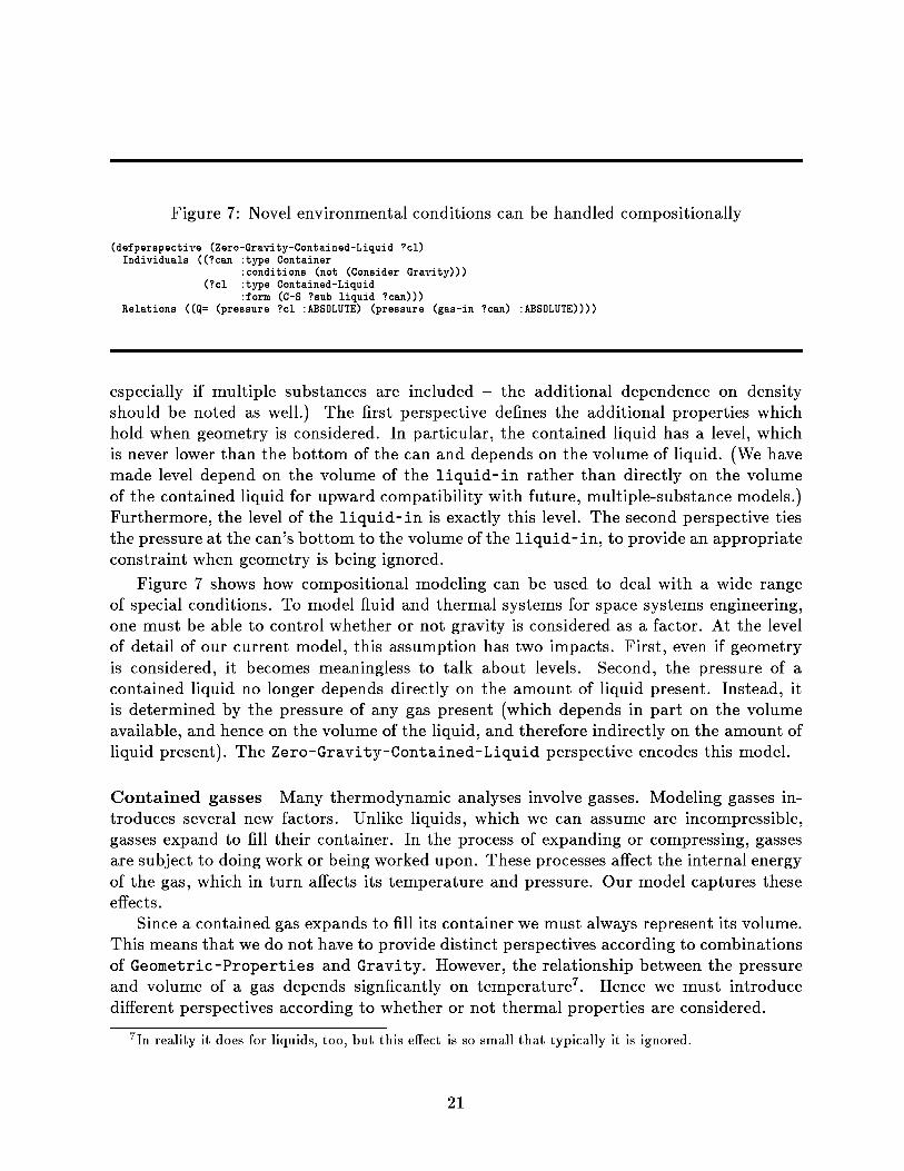
Figure 7 : Novel environmental conditions can be handled compositionally

(defperspective (Zero-Gravity-Contained-Liquid ?cl)Individuals ((?can type Container

conditions (not (Consider Gravity)))(?cl

type Contained-Liquidform (C-S ?sub liquid ?can)))

Relations ((Q= (pressure ?cl :ABSOLUTE) (pressure (gas-in ?can) :ABSOLUTE))))

especially if multiple substances are included – the additional dependence on densityshould be noted as well .) The first perspective defines the additional properties whichhold when geometry is considered . In particular, the contained liquid has a level, whichis never lower than the bottom of the can and depends on the volume of liquid . (We havemade level depend on the volume of the liquid-in rather than directly on the volumeof the contained liquid for upward compatibility with future, multiple-substance models .)Furthermore, the level of the liquid-in is exactly this level . The second perspective tiesthe pressure at the can's bottom to the volume of the liquid-in, to provide an appropriateconstraint when geometry is being ignored.

Figure 7 shows how compositional modeling can be used to deal with a wide rangeof special conditions . To model fluid and thermal systems for space systems engineering,one must be able to control whether or not gravity is considered as a factor . At the levelof detail of our current model, this assumption has two impacts . First, even if geometryis considered, it becomes meaningless to talk about levels . Second, the pressure of acontained liquid no longer depends directly on the amount of liquid present . Instead, itis determined by the pressure of any gas present (which depends in part on the volumeavailable, and hence on the volume of the liquid, and therefore indirectly on the amount ofliquid present) . The Zero-Gravity-Contained-Liquid perspective encodes this model.

Contained gasses Many thermodynamic analyses involve gasses . Modeling gasses in-troduces several new factors . Unlike liquids, which we can assume are incompressible,gasses expand to fill their container . In the process of expanding or compressing, gassesare subject to doing work or being worked upon . These processes affect the internal energyof the gas, which in turn affects its temperature and pressure . Our model captures theseeffects.

Since a contained gas expands to fill its container we must always represent its volume.This means that we do not have to provide distinct perspectives according to combinationsof Geometric-Properties and Gravity . However, the relationship between the pressureand volume of a gas depends signficantly on temperature 7 . Hence we must introducedifferent perspectives according to whether or not thermal properties are considered.

7 In reality it does for liquids, too, but this effect is so small that typically it is ignored.

21

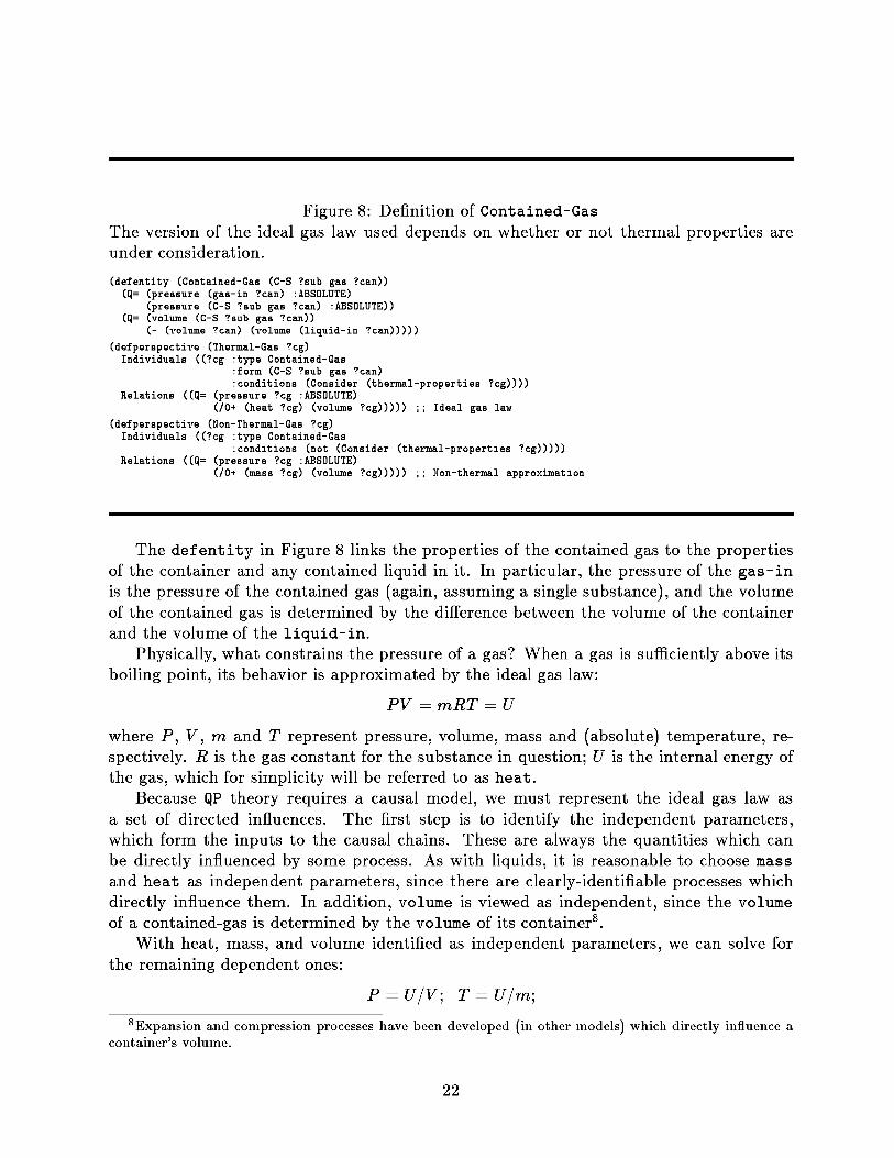
Figure 8 : Definition of Contained-Gas

The version of the ideal gas law used depends on whether or not thermal properties areunder consideration.

(defentity (Contained-Gas (C-S ?sub gas ?can))(Q= (pressure (gas-in ?can) :ABSOLUTE)

(pressure (C-S ?sub gas ?can) :ABSOLUTE))(Q= (volume (C-S ?sub gas ?can))

(- (volume ?can) (volume (liquid-in ?can)))))

(defperspective (Thermal-Gas ?cg)Individuals ((?cg type Contained-Gas

form (C-S ?sub gas ?can)conditions (Consider (thermal-properties ?cg))))

Relations ((Q= (pressure ?cg :ABSOLUTE)(/0+ (heat ?cg) (volume ?cg))))) ; ; Ideal gas law

(defperspective (Non-Thermal-Gas ?cg)Individuals ((?cg type Contained-Gas

conditions (not (Consider (thermal-properties ?cg)))))Relations ((Q= (pressure ?cg :ABSOLUTE)

(/0+ (mass ?cg) (volume ?cg))))) ; ; Non-thermal approximation

The def entity in Figure 8 links the properties of the contained gas to the propertiesof the container and any contained liquid in it . In particular, the pressure of the gas-in

is the pressure of the contained gas (again, assuming a single substance), and the volumeof the contained gas is determined by the difference between the volume of the containerand the volume of the liquid-in.

Physically, what constrains the pressure of a gas? When a gas is sufficiently above itsboiling point, its behavior is approximated by the ideal gas law:

PV = mRT = U

where P, V, m and T represent pressure, volume, mass and (absolute) temperature, re-spectively. R is the gas constant for the substance in question ; U is the internal energy ofthe gas, which for simplicity will be referred to as heat.

Because QP theory requires a causal model, we must represent the ideal gas law asa set of directed influences . The first step is to identify the independent parameters,which form the inputs to the causal chains . These are always the quantities which canbe directly influenced by some process . As with liquids, it is reasonable to choose mass

and heat as independent parameters, since there are clearly-identifiable processes whichdirectly influence them. In addition, volume is viewed as independent, since the volume

of a contained-gas is determined by the volume of its container 8 .With heat, mass, and volume identified as independent parameters, we can solve for

the remaining dependent ones :

P = U/V ; T = Ulm;

'Expansion and compression processes have been developed (in other models) which directly influence acontainer's volume .

22

The constant R is dropped since it does not affect the qualitative behavior of a gas . Theequation for temperature is the same constraint already imposed by Complex-Physob.

Since contained stuffs are already Volumetric-Physobs (see Figure 5) and consideringthermal properties makes them Complex-Physobs (see Figure 2), temperature is alreadyappropriately constrained.

The expression for pressure may seem unintuitive, since it involves neither temperaturenor mass . Intuitively, when gas is added to a closed container, or when a contained gasis heated, the pressure of the gas increases . But in both cases heat is being added tothe gas while its volume remains constant . The model predicts that if the amount of thegas could be increased while its heat is held constant (say by adding gas at absolute zerotemperature), then the pressure would remain unchanged . This result does not conflictwith an intuitive view based on a product of mass and temperature, since the temperaturein the this case would be decreasing, and the net influence on pressure would be ambiguous.

Figure 8 also encodes this analysis using two perspectives . The Thermal-Gas perspec-tive defines the pressure of the gas as the ratio of heat and volume (through the Q=//0+combination) . 9 Thus if the volume of the contained gas is decreased and/or its heat in-creased, the pressure will increase . This corresponds with the result derived from the idealgas law . The Non-Thermal-Gas perspective is similar, but defines the pressure of the gasas the quotient of mass and volume . This is the most reasonable approximation availablewhen thermal properties are not being considered.

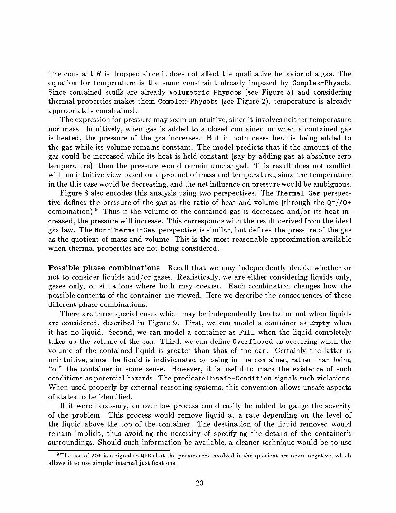
Possible phase combinations Recall that we may independently decide whether ornot to consider liquids and/or gases . Realistically, we are either considering liquids only,gases only, or situations where both may coexist. Each combination changes how thepossible contents of the container are viewed . Here we describe the consequences of thesedifferent phase combinations.

There are three special cases which may be independently treated or not when liquidsare considered, described in Figure 9 . First, we can model a container as Empty whenit has no liquid. Second, we can model a container as Full when the liquid completelytakes up the volume of the can . Third, we can define Overflowed as occurring when thevolume of the contained liquid is greater than that of the can . Certainly the latter isunintuitive, since the liquid is individuated by being in the container, rather than being"of" the container in some sense . However, it is useful to mark the existence of suchconditions as potential hazards . The predicate Unsafe-Condition signals such violations.When used properly by external reasoning systems, this convention allows unsafe aspectsof states to be identified.

If it were necessary, an overflow process could easily be added to gauge the severityof the problem. This process would remove liquid at a rate depending on the level ofthe liquid above the top of the container . The destination of the liquid removed wouldremain implicit, thus avoiding the necessity of specifying the details of the container'ssurroundings . Should such information be available, a cleaner technique would be to use

'The use of /0+ is a signal to QPE that the parameters involved in the quotient are never negative, whichallows it to use simpler internal justifications .

23

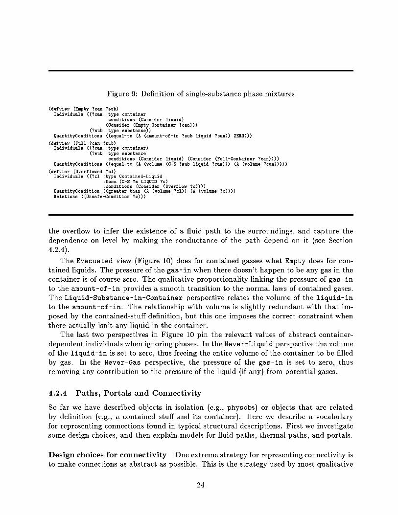
Figure 9 : Definition of single-substance phase mixtures

(defview (Empty ?can ?sub)Individuals ((?can type container

conditions (Consider liquid)(Consider (Empty-Container ?can)))

(?sub type substance))QuantityConditions ((equal-to (A (amount-of-in ?sub liquid ?can)) ZERO)))

(defview (Full ?can ?sub)Individuals ((?can type container)

(?sub type substanceconditions (Consider liquid) (Consider (Full-Container ?can))))

QuantityConditions ((equal-to (A (volume (C-S ?sub liquid ?can))) (A (volume ?can)))))

(defview (Overflowed ?cl)Individuals ((?cl type Contained-Liquid

form (C-S ?s LIQUID ?c)conditions (Consider (Overflow ?c))))

QuantityCondition ((greater-than (A (volume ?cl)) (A (volume ?c))))Relations ((Unsafe-Condition ?c)))

the overflow to infer the existence of a fluid path to the surroundings, and capture thedependence on level by making the conductance of the path depend on it (see Section4 .2.4.

The Evacuated view (Figure 10) does for contained gasses what Empty does for con-tained liquids . The pressure of the gas-in when there doesn't happen to be any gas in thecontainer is of course zero . The qualitative proportionality linking the pressure of gas-in

to the amount-of-in provides a smooth transition to the normal laws of contained gases.The Liquid-Substance-in-Container perspective relates the volume of the liquid-in

to the amount-of-in . The relationship with volume is slightly redundant with that im-posed by the contained-stuff definition, but this one imposes the correct constraint whenthere actually isn't any liquid in the container.

The last two perspectives in Figure 10 pin the relevant values of abstract container-dependent individuals when ignoring phases . In the Never-Liquid perspective the volumeof the liquid-in is set to zero, thus freeing the entire volume of the container to be filledby gas . In the Never-Gas perspective, the pressure of the gas-in is set to zero, thusremoving any contribution to the pressure of the liquid (if any) from potential gases.

4 .2 .4 Paths, Portals and Connectivity

So far we have described objects in isolation (e .g ., physobs) or objects that are relatedby definition (e .g., a contained stuff and its container) . Here we describe a vocabularyfor representing connections found in typical structural descriptions . First we investigatesome design choices, and then explain models for fluid paths, thermal paths, and portals.

Design choices for connectivity One extreme strategy for representing connectivity isto make connections as abstract as possible . This is the strategy used by most qualitative

24

Figure 10: Definition of single-substance mixtures, continued

(defview (Evacuated ?can ?sub)Individuals ((?can type container)

(?sub type substanceconditions (Consider gas)(Quantity (Amount-of-in ?sub gas ?can))))

QuantityConditions ((equal-to (A (amount-of-in ?sub gas ?can)) ZERO))Relations ((equal-to (A (pressure (gas-in ?can) :ABSOLUTE)) ZERO)

(Qprop+ (pressure (gas-in ?can) :ABSOLUTE)(amount-of-in ?sub gas ?can))))

(defperspective (Liquid-Substance-in-Container ?can ?sub)Individuals ((?can type container

conditions (Consider liquid))(?sub type substance))

Relations ((Qprop+ (volume (liquid-in ?can)) (amount-of-in ?sub liquid ?can))(Ordered-Correspondence ((A (volume (liquid-in ?can))) ZERO) ; ; Single-Substance Asn

((A (amount-of-in ?sub liquid ?can)) ZERO))))

(defperspective (never-liquid ?can)Individuals ((?can type container

conditions (not (consider liquid))))Relations ((equal-to (A (volume (liquid-in ?can))) ZERO)))

(defperspective (never-gas ?can)Individuals ((?can :type container

:conditions (not (consider gas))))Relations ((equal-to (A (pressure (gas-in ?can) :ABSOLUTE)) ZERO)))

models, including non-QP models . However, this strategy has several limitations . First, it

does not explicitly represent the fact that there can be different kinds of stuff inside a path

at distinct times . This is not a problem if real fluids can be accurately modeled as abstract

stuffs, as system-dynamics models do [2] . Anyone who has tried debugging plumbing

systems, however, knows that this is often not always a realistic approximation! Second,

the purely abstract path representation does not allow the geometry of the container and

the arrangements of stuffs inside to be taken into account . A hole drilled in the middle of

a water tank, for example, will not drain it completely, while a hole drilled on the bottom

will . For some problems, the ability to reason about the geometry of the piping system is

essential.

Our model abstracts all structural objects into two kinds: containers and paths which

connect them. Every fluid path connects exactly two distinct containers . Abstract nodes,

commonly used in modeling electrical circuits, are not allowed . The reason is that they are

inconsistent with our view of causality as unidirectional and loop—free . To see this, imagine

glueing together three pipes in series . The resulting assembly should behave as a single

pipe. The problem is that there is no consistent rendering of causal directedness which

can account for the pressures at the internal nodes . For example, if one end of the pipe

sees an increasing pressure while the other end sees a decreasing pressure, the pressures

at the internal nodes will be ambiguous . This could be explained by having each node

determine its pressure by looking at its two adjacent nodes . But this requires causality to

run in both directions through the center pipe, which is unintuitive.

25

It is therefore necessary to model nodes in a piping system as containers, whose pres-sures vary with the amount of fluid present . This choice has the disadvantage that onemust deal with extra contained stuffs . More significantly, a node modeled as an accu-mulator does not obey Kirchoff's Current Law—in general, the flow out will not equalthe flow in. New (and often unwanted) behaviors emerge as node pressures rise and fall.One solution is to "pre-assemble" multiple pipes into a single path, and model the systemaccordingly . This is part of a larger problem of mapping structural descriptions to struc-tural abstractions. At present, this is done manually . A second alternative, common inengineering analyses, is to only consider steady-state behaviors (see Section 4 .5 .1).

We introduce the idea of a portal to reason about the geometry of stuffs inside acontainer . Many problems do not require the level of detail represented by portals . Conse-quently, we use modeling assumptions to control whether or not portals are introduced forany particular analysis . If the assumption (Consider Portals) is false, the QP interpreteruses a more abstract model of path.

Another design choice concerns the representation of conductance . In physics, con-ductance refers to how easily stuff can flow through a path . In a qualitative physics,conductance shows up as a factor affecting rates associated with flow processes . Conduc-tance can be modeled in two ways . The first is not to represent it at all . Many qualitativeanalyses are concerned with making broad predictions about systems having only fixedconductances, so the particular value is irrelevant . The second choice is to introduce anexplicit quantity for a path's conductance . This provides more accurate credit assignmentif one is performing a comparative analysis . Our model provides both options, controlledby the modeling assumption (Consider (fluid-conductance ?path)) . The assumption(Consider (thermal-conductance ?path)) plays a similar role for heat paths.

Finally, it is often convenient to place restrictions on what kinds of stuff can flowthrough particular paths and in what directions . For instance, some piping systems havecheck valves which prevent liquid from flowing in one direction . An open trough leadingfrom one container to another works perfectly well as a path for liquids, but will notsuccessfully convey air between them . Our vocabulary for connections includes restrictionswhich can be used to model situations like these.

A purist might insist that scenario modelers always resort to a CAD-style encodingof a structural description, and derive restrictions on the kinds of flows which can occurthrough paths based on a "first principles" analysis . We lean towards this view ourselves,but also recognize that (a) scenario modelers have a hard enough job as it is withoutus making it harder for them; and (b) such a first principles analysis will need a set ofdistinctions like ours to express the results of their derivations anyway.

We assume that consistency tests on structural descriptions, such as ensuring thateach path only connects to two components, are carried out by a preprocessor . It wouldbe easy to install such checks in the domain model, but separating them makes more sensepragmatically because their encoding depends on interface issues as well as inferential ones.

Fluid paths Figure 11 provides the starting point for the definition of fluid paths . Allfluid paths are physobs, as enforced by the first defentity . A fluid path is a gas-path if it

26

Figure 11 : Definition for Fluid—Paths

(defentity Fluid-Path (Physob ?self))

(defperspective (General-Fluid-Path ?path)Individuals ((?path type fluid-path

conditions (Consider capable-fluid-paths))))

(defperspective (Liquid-Path ?path)Individuals ((?path type general-fluid-path

conditions (Consider liquid))))

(defentity Liquid-Path (Possible-Path-Phase ?self liquid))

(defperspective (Gas-Path ?path)Individuals ((?path type general-fluid-path

conditions (Consider gas))))

(defentity Gas-Path (Possible-Path-Phase ?self gas))

(defpredicate (Possible-Path-Phase ?path ?st)(Fluid-Path ?path)(Consider ?st))

Figure 12: Defining connections

(defpredicate (Fluid-Connection ?path ?from ?to)(Connects-To ?path ?from ?to) (Connects-To ?path ?to ?from))

(defpredicate (Connects-To ?path ?from ?to)(Path-Container ?path ?from)

(Path-Container ?path ?to))

allows gasses to flow, a liquid-path if it allows liquids to flow, and a General-Fluid-Pathif it allows both liquids and gasses to flow.

The representation of single-substance paths might seem overly complicated, but isnecessary to provide flexibility for scenario modelers . The first perspective allows themodeler to declare all fluid paths to be general fluid paths, by assuming (Considercapable-fluid-paths).

Recall that a modeler may choose independently whether or not to consider gasses orliquids in a particular analysis . If one is considering liquids and not gasses, say, then ageneral-fluid-path should only act as a liquid path and not as a gas path . The next twoperspectives in Figure 11 provide this ability . Finally, the predicate Possible-Path-Phaseprovides a functional encoding of the phase(s) which a particular path is allowed to carry.This is essential for the general-purpose fluid-flow process, described in Section 4 .3.2.

Figure 12 shows the relationships which link a fluid path to its containers . The predicateConnects-To is used by flow processes to establish whether or not fluid can flow in aparticular direction . Thus the modeler can declare a unidirectional path by asserting asingle instance of Connects-To . Since Fluid-Connection implies Connects-To in both

27

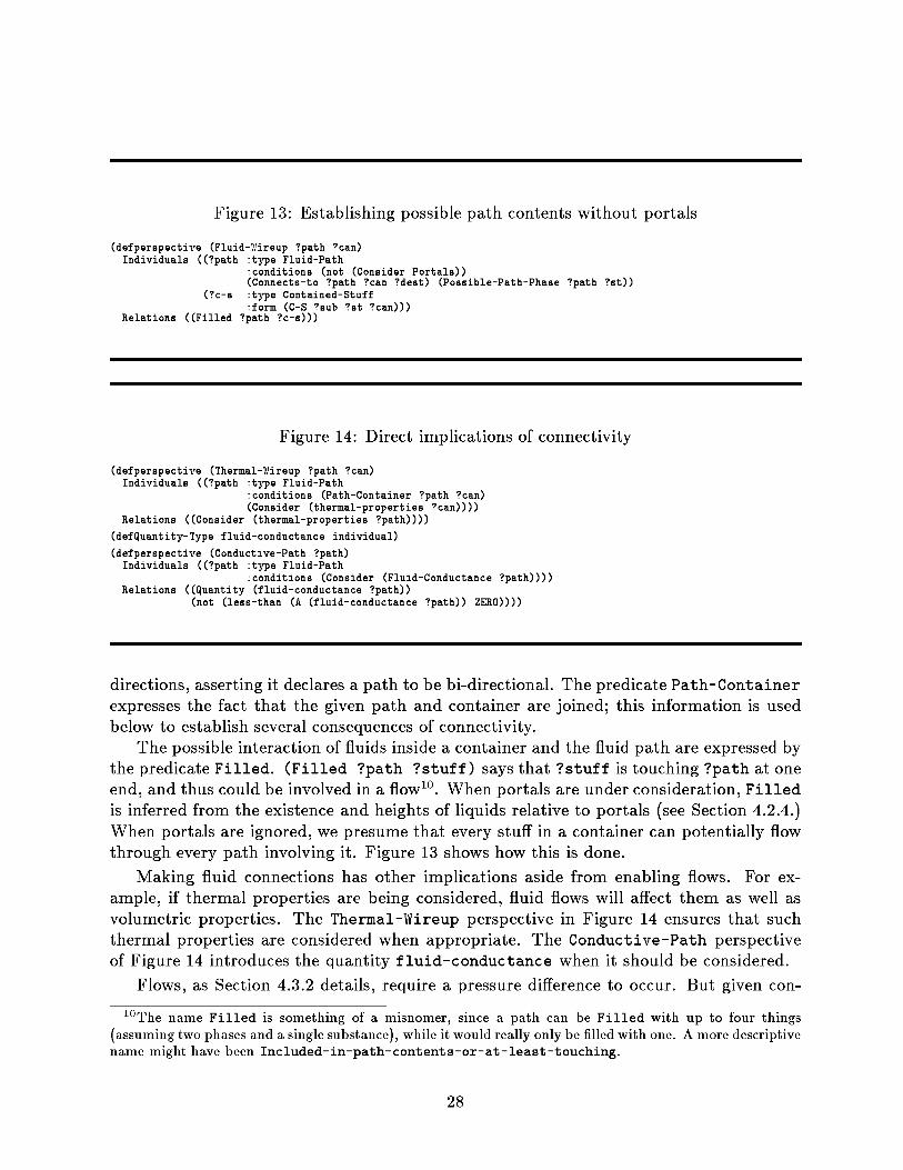
Figure 13 : Establishing possible path contents without portals

(defperspective (Fluid-Wireup ?path ?can)Individuals ((?path type Fluid-Path

conditions (not (Consider Portals))(Connects-to ?path ?can ?dent) (Possible-Path-Phase ?path ?st))

(?c-s

type Contained-Stuffform (C-S ?sub ?st ?can)))

Relations ((Filled ?path ?c-s)))

Figure 14 : Direct implications of connectivity

(defperspective (Thermal-Wireup ?path ?can)Individuals ((?path type Fluid-Path

conditions (Path-Container ?path ?can)(Consider (thermal-properties ?can))))

Relations ((Consider (thermal-properties ?path))))

(defQuantity-Type fluid-conductance individual)

(defperspective (Conductive-Path ?path)Individuals ((?path type Fluid-Path

conditions (Consider (Fluid-Conductance ?path))))Relations ((Quantity (fluid-conductance ?path))

(not (less-than (A (fluid-conductance ?path)) ZERO))))

directions, asserting it declares a path to be bi-directional . The predicate Path-Containerexpresses the fact that the given path and container are joined ; this information is usedbelow to establish several consequences of connectivity.

The possible interaction of fluids inside a container and the fluid path are expressed bythe predicate Filled. (Filled ?path ?stuff) says that ?stuff is touching ?path at oneend, and thus could be involved in a flow 10. When portals are under consideration, Filledis inferred from the existence and heights of liquids relative to portals (see Section 4 .2 .4 .)When portals are ignored, we presume that every stuff in a container can potentially flowthrough every path involving it . Figure 13 shows how this is done.

Making fluid connections has other implications aside from enabling flows . For ex-ample, if thermal properties are being considered, fluid flows will affect them as well asvolumetric properties. The Thermal-Wireup perspective in Figure 14 ensures that suchthermal properties are considered when appropriate . The Conductive-Path perspectiveof Figure 14 introduces the quantity fluid-conductance when it should be considered.

Flows, as Section 4.3 .2 details, require a pressure difference to occur . But given con-

'The name Filled is something of a misnomer, since a path can be Filled with up to four things(assuming two phases and a single substance), while it would really only be filled with one . A more descriptivename might have been Included-in-path-contents-or-at-least-touching.

28

Figure 15: Selecting which pressure to use in inferring flow

(defperspective (Pressure-Definer ?path ?can (bottom ?can))Individuals ((?path :type Fluid-Path

:conditions (Path-Container ?path ?can) (not (Consider Portals)))))

tainers which can hold more than one contained stuff, how do we know which pressure touse?

Recall that the abstract individuals liquid-in and gas-in gave us a more modular wayto represent the properties of mixtures in a container . Similarly, we introduce the notionof a Pressure-Definer as a source of information about pressures to insulate us fromwhether or not we are using portals. This insulation greatly simplifies the description ofmaterial flows . (pressure-definer ?path ?can ?obj) means that ?obj should be theentity whose pressure is used as the pressure of ?can for ?path . Since every path hasexactly two distinct containers, there will be two distinct pressure-definers for eachpath . Figure 15 shows the simplest approximation for pressure definers : When no otherinformation is available, use the pressure at the bottom of the container . Physically, thisis tantamount to restricting all fluid paths to connect to bottoms of containers.

Heat paths Heat paths (see Figure 16) connect two distinct simple-thermal-physobs-that is, physical objects which have a temperature. Heat paths are simpler than fluid pathsbecause (a) internal energy doesn't come in phases and (b) geometry (at least in this levelof modeling) is irrelevant' . Thermally-Connects-To indicates one-way connections l2 ,

and Heat-Connection indicates bidirectional thermal paths . thermal-conductance rep-resents a path's ability to transmit heat . As with fluid-conductance, the introductionof thermal conductance is controlled by a modeling assumption.

Valves Valves are employed to regulate or restrict flows through paths . The simplestmodel of a valve is binary, providing an on/off switch for fluid flow . This level of modelcan easily be achieved by introducing Blocked (see below) as an explicit assumption on afluid path and using actions to correspond to changing its state [7], so we do not discussit further. A slightly more complex model has valves affecting the conductance of a path.

11In a more detailed model heat paths would be inferred from the geometry of the system and the existenceof stuffs, and the conductance would depend on the nature and geometry of the stuff providing a physicalconnection . However, we include so little information about materials and container geometry that thisadditional level of detail would be useless . Whole textbooks are written on heat transfer, which analyzespecial cases analytically and describe how to use finite element methods to derive numerical solutions formore realistic shapes . We suspect that there may be one or two useful levels of detail between this modeland a quantitative geometry, but that the extra leverage they provide is not very high.

'We are not arguing for the existence of thermal check-valves ; rather, we include one-way heat paths toallow control over the model .

29

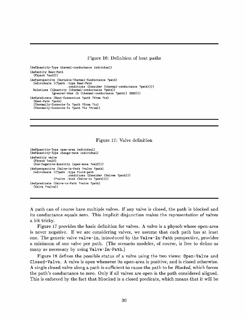
Figure 16: Definition of heat paths

(defQuantity-Type thermal-conductance individual)

(defentity Heat-Path(Physob ?self))

(defperspective (Variable-Thermal-Conductance ?path)Individuals ((?path type Heat-Path

conditions (Consider (thermal-conductance ?path))))Relations ((Quantity (thermal-conductance ?path))

(greater-than (A (thermal-conductance ?path)) ZERO)))

(defpredicate (Heat-Connection ?path ?from ?to)(Heat-Path ?path)(Thermally-Connects-To ?path ?from ?to)(Thermally-Connects-To ?path ?to ?from))

Figure 17 : Valve definition

(defQuantity-Type open-area individual)(defQuantity-Type change-rate individual)

(defentity valve(Physob ?self)(Non-Negative-Quantity (open-area ?self)))

(defperspective (Valve-in-Path ?valve ?path)Individuals ((?path type fluid-path

conditions (Consider (Valves ?path)))(?valve bind (Valve-in ?path))))

(defpredicate (Valve-in-Path ?valve ?path)(Valve ?valve))

A path can of course have multiple valves . If any valve is closed, the path is blocked andits conductance equals zero . This implicit disjunction makes the representation of valvesa bit tricky.

Figure 17 provides the basic definition for valves . A valve is a physob whose open-areais never negative . If we are considering valves, we assume that each path has at leastone . The generic valve valve-in, introduced by the Valve-In-Path perspective, providesa minimum of one valve per path . (The scenario modeler, of course, is free to define asmany as necessary by using Valve-In-Path .)

Figure 18 defines the possible status of a valve using the two views : Open-Valve andClosed-Valve . A valve is open whenever its open-area is positive, and is closed otherwise.A single closed valve along a path is sufficient to cause the path to be Blocked, which forcesthe path's conductance to zero. Only if all valves are open is the path considered aligned.This is enforced by the fact that Blocked is a closed predicate, which means that it will be

30

Figure 18 : Valve status

(defview (Open-Valve ?valve)Individuals ((?valve type Valve

conditions (Valve-In-Path ?valve ?path)(Consider (Valves ?path))))

QuantityConditions ((greater-than (A (open-area ?valve)) ZERO)))

(defview (Closed-Valve ?valve)Individuals ((?valve type Valve

conditions (Valve-In-Path ?valve ?path)(Consider (Valves ?path))))

QuantityConditions ((equal-to (A (open-area ?valve)) ZERO))Relations ((Blocked ?path)

(equal-to (A (conductance ?path)) ZERO)))

(defClosed-Predicate Blocked)

(defperspective (Aligned ?path)Individuals ((?path :type Fluid-Path

:conditions (not (Blocked ?path))))Relations ((only-during (greater-than (A (conductance ?path)) ZERO))))

assumed to be false for all conditions in which it is not known to be true . That is, unlessone knows of a closed valve, one assumes that the path is aligned.

Figure 19 defines a process for changing a valve's status . When considering Changing-Valves, a valve has a change-rate quantity which directly influences its open-area . Thetwo views—Opening-Valve and Closing-Valve—are used to distinguish the possible di-rections of change. The model provides no constraint on the change-rate, so the scenariomay constrain it as desired . The Changing-Conductance perspective relates a valve'sopen-area to the conductance of its fluid-path, as long as the path is aligned . Modelingmany control systems requires modeling valves whose state is linked to system parame-ters. This model can be modified to suit this purpose by (a) adding a precondition to theChanging-Valves process, controlled by other processes or views, which determines whenit is acting and (b) by imposing the appropriate sign constraints on the change-rate.

Portals The abstract model of containers and paths suffices for many problems . How-ever, sometimes it is important to represent the geometry of the interface between pathsand containers . If there are two holes in a water tank at different heights, for example, weknow the higher one will run dry before the lower one . If we are trying to siphon waterout of a tub, it is important to keep the inlet of the siphon below the water line . Followingthe terminology used by Hayes [10], we call these interfaces portals.

We consider portals to be distinct entities, whose existence depends on the connectionbetween some form of fluid path and a container . The function PT maps from containersand paths to portals . That is, (PT ?can ?path) refers to the portal formed by connect-ing ?path to ?can. Clearly this encoding is unable to distinguish the portals of a pathconnected to the same container at both ends ; fortunately this situation rarely arises inengineered fluid and thermal systems .

31

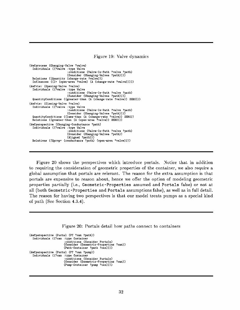
Figure 19 : Valve dynamics

(defprocess (Changing-Valve ?valve)Individuals ((?valve type Valve

conditions (Valve-In-Path ?valve ?path)(Consider (Changing-Valves ?path))))

Relations ((Quantity (change-rate ?valve)))Influences ((I+ (open-area ?valve) (A (change-rate ?valve)))))

(defview (Opening-Valve ?valve)Individuals ((?valve type Valve

conditions (Valve-In-Path ?valve ?path)(Consider (Changing-Valves ?path))))

QuantityConditions ((greater-than (A (change-rate ?valve)) ZERO)))

(defview (Closing-Valve ?valve)Individuals ((?valve type Valve

conditions (Valve-In-Path ?valve ?path)(Consider (Changing-Valves ?path))))

QuantityConditions ((less-than (A (change-rate ?valve)) ZERO))Relations ((greater-than (A (open-area ?valve)) ZERO)))

(defperspective (Changing-Conductance ?path)Individuals ((?valve type Valve

conditions (Valve-In-Path ?valve ?path)(Consider (Changing-Valves ?path))(Aligned ?path)))

Relations ((Qprop+ (conductance ?path) (open-area ?valve))))

Figure 20 shows the perspectives which introduce portals . Notice that in additionto requiring the consideration of geometric properties of the container, we also require aglobal assumption that portals are relevant . The reason for the extra assumption is thatportals are expensive to reason about, hence we offer the option of modeling geometricproperties partially (i .e ., Geometric-Properties assumed and Portals false) or not atall (both Geometric-Properties and Portals assumptions false), as well as in full detail.The reason for having two perspectives is that our model treats pumps as a special kindof path (See Section 4 .3.4).

Figure 20 : Portals detail how paths connect to containers

(defperspective (Portal (PT ?can ?path))Individuals ((?can type Container

conditions (Consider Portals)(Consider (Geometric-Properties ?can))(Path-Container ?path ?can))))

(defperspective (Portal (PT ?can ?pump))Individuals ((?can type Container

conditions (Consider Portals)(Consider (Geometric-Properties ?can))(Pump-Container ?pump ?can))))

32

Figure 21 : Properties of portals

(defentity (Portal (PT ?can ?path))(Quantity (height (PT ?can ?path) ?pt))(not (less-than (A (height (PT ?can ?path))) (A (height (bottom ?can)))))(not (greater-than (A (height (PT ?can ?path))) (A (height (top ?can)))))(Quantity (pressure (PT ?can ?path)))(Quantity (pressure (PT ?can ?path) (gas-in ?can)))(Q= (pressure (PT ?can ?path) :ABSOLUTE)

(+ (pressure (gas-in ?can) :ABSOLUTE)(pressure (PT ?can ?path) (gas-in ?can)))))

(defperspective (pressure-definer ?path ?can ?pt)Individuals ((?pt type portal

form (PT ?can ?path)conditions (Consider Portals))))

The basic properties of portals are defined in Figure 21 . A portal has a height, which

is constrained to lie between the container's top and bottom . It has a pressure, which

is defined as the pressure of the container's gas-in plus the pressure contributed by the

weight of any liquid above the portal . The latter is represented as (pressure ?pt (gas-in

?can)), e.g ., the difference between the portal pressure and the pressure of the gas-in.This simple definition of pressure puts the complexity elsewhere, namely in the definition

of the constituent pressures.

Given that we are considering only single-substance systems, a portal is in contact with

Figure 22 : Describing what touches a portal

(defview (Submerged-in ?pt ?cl)Individuals ((?cl type contained-liquid

form (C-S ?sub liquid ?can))(?pt type portal

form (PT ?can ?path)))QuantityConditions ((greater-than (A (level ?cl)) (A (height ?pt))))Relations ((only-during (Filled ?path ?cl))

(only-during (Exposed-to ?pt ?cl))(Qprop+ (pressure ?pt (gas-in ?can)) (level ?cl))(greater-than (A (pressure ?pt (gas-in ?can))) ZERO)))

(defview (Dry-Portal ?pt)Individuals ((?pt type portal

form (PT ?can ?path)))QuantityConditions ((not (greater-than (A (level (liquid-in ?can))) (A (height ?pt)))))Relations ((equal-to (A (pressure ?pt (gas-in ?can))) ZERO)))

(defperspective (Exposed-to ?pt ?cg)Individuals ((?cg type contained-gas

form (C-S ?sub gas ?can))(?pt type Dry-Portal

form (PT ?can ?path)))Relations ((only-during (Filled ?path ?cg))))

33

Figure 23: Relating pressures of portals in the same container

(defPerspective (Common-Portals ?ptl ?pt2)Individuals ((?ptl type Portal

form (PT ?can ?pathl))(?pt2 type Portal

form (PT ?can ?path2)test (alphalessp ?pathl ?path2)))

Relations ((Ordered-Correspondence((A (pressure ?ptl :ABSOLUTE))

(A (pressure ?pt2 :ABSOLUTE)))((A (pressure ?ptl (gas-in ?can))) (A (pressure ?pt2 (gas-in ?can)))))))

(defPerspective (Common-Submerged-Portals ?ptl ?pt2)Individuals ((?ptl type Submerged-Portal

form (PT ?can ?pathl)conditions (Common-Portals ?ptl (PT ?can ?path2)))

(?pt2 type Submerged-Portalform (PT ?can ?path2)))

Relations ((Ordered-Correspondence((A (pressure ?ptl (gas-in ?can))) (A (pressure ?pt2 (gas-in ?can))))((A (height ?pt2))

(A (height ?ptl))))))

either a contained gas, a contained liquid, or neither . Since we are approximating portalsby only a single height, we ignore the fact that in real portals there are times when boththe liquid and gas would be in contact, as the interface between them moves between theheights of the top and bottom of the portal.

The view Submerged-In describes the case where the portal is in contact with liquid.This occurs when the portal's height is lower than the liquid's level . When the portalis submerged, we stipulate that the path is Filled with the liquid (See Section 4 .2 .4).(Notice that this model ignores the possibility of complicated geometry in the fluid paths,which would allow part of a piping system to remain empty while another part is full . Wehave not delved into this level of detail because the contained-stuff ontology is not suitablefor representing finite-sized "chunks" of stuff (i .e., bubbles) inside a fluid path .) When aportal is submerged, the pressure contributed by the liquid above it is positive, and is anincreasing function of the level.

The view Dry-Portal describes the case where the portal is not submerged . The factthat there is no liquid above the portal is reflected by the constraint that the pressure ofthe portal relative to the gas pressure is equal to zero. Notice that being dry does notnecessarily imply that the portal is in contact with a gas, since there might not be anygas in the container . The consequence of dryness when gas is present is represented bythe Exposed-To perspective, namely that the path is then Filled with the gas . A subtlepoint: Notice that Dry-Portal is predicated on the level of Liquid-In . This means thatit will hold even when liquids are not considered (recall the Empty and Never-Liquid

perspectives), and so in that case every portal will touch the gas of its container, if any.

To weed out any violations in transitivity, it is important to ensure that as manyinequality relations of interest are derivable as possible . Figure 23 shows how this is donefor two portals sharing a common container . The contribution to each portal's pressure

34

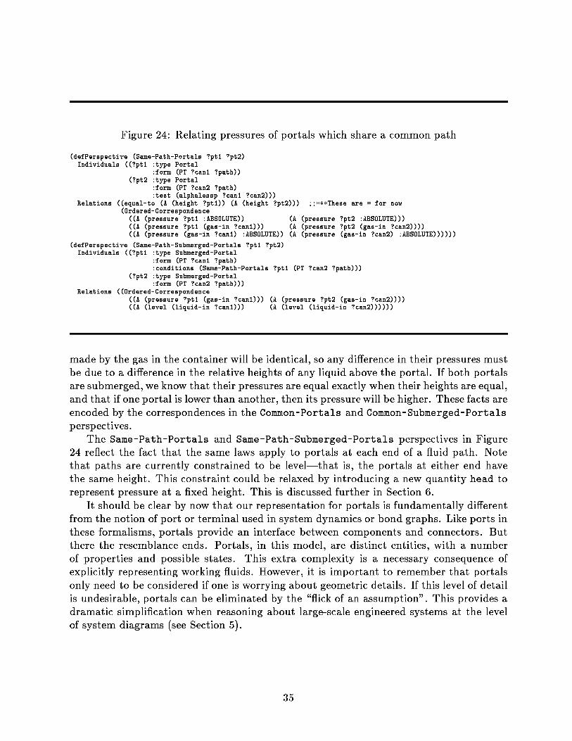
Figure 24 : Relating pressures of portals which share a common path

(defPerspective (Same-Path-Portals ?ptl ?pt2)Individuals

((?ptl

(?pt2

Relations

((equal-to

typeformtypeformtest(A

Portal(PT ?canl ?path))Portal(PT ?can2 ?path)(alphalessp ?canl ?can2)))

; ;***These are = for now(height

?ptl))

(A

(height

?pt2)))(Ordered-Correspondence

((A (pressure

?ptl

:ABSOLUTE))

(A (pressure ?pt2

:ABSOLUTE)))((A (pressure

?ptl

(gas-in ?canl)))

(A (pressure ?pt2

(gas-in

?can2))))((A (pressure

(gas-in ?canl)

:ABSOLUTE))

(A (pressure (gas-in ?can2)

:ABSOLUTE))))))

(defPerspective (Same-Path-Submerged-Portals ?ptl ?pt2)Individuals ((?ptl type Submerged-Portal

form (PT ?canl ?path)conditions (Same-Path-Portals ?ptl (PT ?can2 ?path)))

(?pt2 type Submerged-Portalform (PT ?can2 ?path)))

Relations ((Ordered-Correspondence((A (pressure ?ptl (gas-in ?canl))) (A (pressure ?pt2 (gas-in ?can2))))((A (level (liquid-in ?canl)))

(A (level (liquid-in ?can2))))))

made by the gas in the container will be identical, so any difference in their pressures mustbe due to a difference in the relative heights of any liquid above the portal . If both portalsare submerged, we know that their pressures are equal exactly when their heights are equal,and that if one portal is lower than another, then its pressure will be higher . These facts areencoded by the correspondences in the Common-Portals and Common-Submerged-Portalsperspectives.

The Same-Path-Portals and Same-Path-Submerged-Portals perspectives in Figure24 reflect the fact that the same laws apply to portals at each end of a fluid path . Notethat paths are currently constrained to be level—that is, the portals at either end havethe same height . This constraint could be relaxed by introducing a new quantity head torepresent pressure at a fixed height . This is discussed further in Section 6.

It should be clear by now that our representation for portals is fundamentally differentfrom the notion of port or terminal used in system dynamics or bond graphs . Like ports inthese formalisms, portals provide an interface between components and connectors . Butthere the resemblance ends . Portals, in this model, are distinct entities, with a numberof properties and possible states . This extra complexity is a necessary consequence ofexplicitly representing working fluids . However, it is important to remember that portalsonly need to be considered if one is worrying about geometric details . If this level of detailis undesirable, portals can be eliminated by the "flick of an assumption" . This provides adramatic simplification when reasoning about large-scale engineered systems at the levelof system diagrams (see Section 5) .

35

Figure 25 : Process Definition for Heat Flow

(defQuantity-Type heat-flow-rate individual)

(defprocess (Heat-Flow ?src ?dst ?path)Individuals ((?path :type heat-path

:conditions (thermally-connects-to ?path ?src ?dst))(?src :type simple-thermal-physob)(?dst :type simple-thermal-physob))

Preconditions ((heat-aligned ?path))QuantityConditions ((greater-than (A (temperature ?src :ABSOLUTE))

(A (temperature ?dst :ABSOLUTE))))Relations ((quantity heat-flow-rate))Influences ((I+ (Heat ?dst) (A heat-flow-rate))

(I- (Heat ?src) (A heat-flow-rate))))

4 .3 Flow Processes

Several thermodynamic processes involve the transfer of material or energy from one lo-cation to another . They have a common pattern . Each involves a source, destination, anda path. Each requires a difference in some parameter (eg ., temperature or pressure) tooccur. Since the contained-stuff ontology does not provide a means to define pieces of stuffindependently from containers, we cannot describe the details of the traversal of stuff fromone place to another . Nor do we need to, for the kinds of systems-level analyses whichmotivate this model . The fact that there is some "stuff" which is conserved during theflow is encoded by the constraints on the source and destination . In particular, each flowprocess has an associated rate, which provides a negative direct influence on some propertyof the source (thus modeling "stuff" leaving the source) and a positive direct influence onsome property of the destination (thus modeling "stuff" entering the destination).

The basic flow processes in this domain model are Heat-Flow and Fluid-Flow . Wedescribe each in turn.

4 .3 .1 Heat Flow

The abstractness of internal energy (no phases, no changes in existence) makes heat flowone of the simplest processes to model . Figure 25 defines the Heat-Flow process . Thesource (?src) and destination (?dst) are both simple-thermal-physobs, which ensuresthey both have temperature . (The astute reader will notice that this does not necessarilyensure that they both have heat . The reason for this is explained below .) They must beconnected by a heat path (?path), as indicated by the individuals specification13

For heat flow to occur, the path must be capable of supporting heat flow (i .e ., heat-aligned)and the temperature in the source must be greater than that of the destination, as thequantity conditions indicate . When heat flow is occuring, heat-flow-rate becomes an

13The order of the specifications is designed for efficient matching.

36

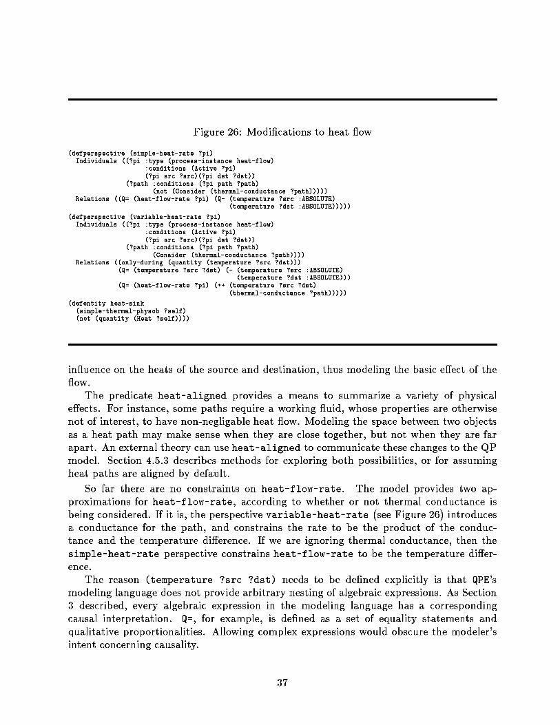
Figure 26: Modifications to heat flow

(defperspective (simple-heat-rate ?pi)Individuals ((?pi type (process-instance heat-flow)

conditions (Active ?pi)(?pi src ?src)(?pi dst ?dst))

(?path :conditions (?pi path ?path)(not (Consider (thermal-conductance ?path)))))

Relations ((Q= (heat-flow-rate ?pi) (Q- (temperature ?src :ABSOLUTE)(temperature ?dst :ABSOLUTE)))))

(defperspective (variable-heat-rate ?pi)Individuals ((?pi type (process-instance heat-flow)

conditions (Active ?pi)(?pi src ?src)(?pi dst ?dst))

(?path :conditions (?pi path ?path)(Consider (thermal-conductance ?path))))

Relations ((only-during (quantity (temperature ?src ?dst)))(Q= (temperature ?src ?dst) (- (temperature ?src :ABSOLUTE)

(temperature ?dst :ABSOLUTE)))(Q= (heat-flow-rate ?pi) (*+ (temperature ?src ?dst)

(thermal-conductance ?path)))))

(defentity heat-sink(simple-thermal-physob ?self)(not (quantity (Heat ?self))))

influence on the heats of the source and destination, thus modeling the basic effect of theflow.

The predicate heat-aligned provides a means to summarize a variety of physicaleffects . For instance, some paths require a working fluid, whose properties are otherwisenot of interest, to have non-negligable heat flow . Modeling the space between two objectsas a heat path may make sense when they are close together, but not when they are farapart . An external theory can use heat-aligned to communicate these changes to the QPmodel . Section 4 .5.3 describes methods for exploring both possibilities, or for assumingheat paths are aligned by default.

So far there are no constraints on heat-flow-rate . The model provides two ap-proximations for heat-flow-rate, according to whether or not thermal conductance isbeing considered . If it is, the perspective variable-heat-rate (see Figure 26) introducesa conductance for the path, and constrains the rate to be the product of the conduc-tance and the temperature difference . If we are ignoring thermal conductance, then thesimple-heat-rate perspective constrains heat-flow-rate to be the temperature differ-ence.

The reason (temperature ?src ?dst) needs to be defined explicitly is that QPE'smodeling language does not provide arbitrary nesting of algebraic expressions . As Section3 described, every algebraic expression in the modeling language has a correspondingcausal interpretation . Q=, for example, is defined as a set of equality statements andqualitative proportionalities . Allowing complex expressions would obscure the modeler'sintent concerning causality.

37

Figure 26 also shows our representation of heat sinks . A heat-sink is a simple-thermal-physobwhich cannot have heat . Being a simple-thermal-physob means that heat sinks can par-ticipate in heat flows . We are exploiting a property of our modeling language : a directinfluence on a parameter which doesn't exist has no effect . Thus the process will have noeffect on the temperature of the sink.

This is not the only way to model such sinks in QP theory. For example, one could usea "replenisher" process which supplies or removes additional heat from the sink to keepits temperature constant . The disadvantage of this scheme is that it requires an extraprocess for each sink. Or, one could define a sink as having both heat and temperature,

but without any causal connection between them . However, unlike the other two schemes,this does not put the heat sink completely outside the modeling realm—for example, if wewish to enforce steady state (see Section 4 .5 .1), we would not want to reject a state simplybecause some heat sink has an increasing heat quantity.

4 .3 .2 Fluid Flow

Models of fluid flow can be extremely complex : Many hours of supercomputer time arecurrently spent solving fluid dynamics problems. As might be expected, our models will bemuch simpler . This simplicity is appropriate given our focus on system-level rather thandetailed "component-level" phenomena . We ignore the dynamics involved in acceleratingthe mass of fluid in the path . We ignore the distinction between turbulent and non-turbulent flow . Even so, the model we have developed contains some (perhaps surprising)sophistications.

Previous QP models have tended to use separate processes to describe the flow of liquidsand the flow of gasses . While simple, it has the disadvantage of obscuring many importantunderlying similarities . Several distinctions introduced earlier, most notably the conceptsof Pressure-Definer and Possible-Path-Phase, allow us to represent the common, corephenomena of fluid flow by a single process . This process is then modified by additionalperspectives which encode the consequences pertaining to liquids or gasses as needed . Inour model these consequences pertain to the interactions of thermal properties with fluidflow. This section describes the basic model, and Section 4 .3.3 describes the associatedthermal model of fluid flow.

Let us examine how this is done in detail . Figure 27 describes the basic fluid flowprocess . The variable ?path is constrained to be a fluid path, which subsumes both liquidand gas paths (recall Figure 11) . The containers attached to the path are ?src and ?dst,as indicated by the connects-to predication . The predication on possible-path-phaseprovides the phase (?st) . The source contained stuff, ?src-cs, has the form (C-S ?sub?st ?src), which must be a contained stuff. Thus for every path which can contain aparticular phase, every distinct substance ?sub would give rise to a distinct instance ofFluid-Flow . (This is for upward compatibility with future models for describing multiple-substance systems .) The trigger involving the destination container ?dst simply ensuresthat it is a container. Given the rest of our current model it must be a container, of course.However, including this individual explicitly allows us to refer to "the destination of a fluid

38

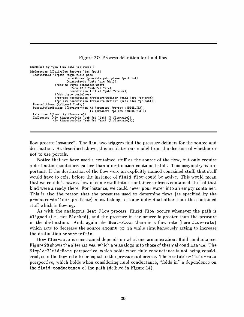
Figure 27: Process definition for fluid flow

(defQuantity-Type flow-rate individual)

(defprocess (fluid-flow ?src-cs ?dst ?path)Individuals ((?path :type fluid-path

:conditions (possible-path-phase ?path ?st)(connects-to ?path ?src ?dst))

(?src-cs type contained-stuffform (C-S ?sub ?st ?src)conditions (Filled ?path ?src-cs))

(?dst :type container)(?pr-src conditions (Pressure-Definer ?path ?src ?pr-src))(?pr-dst conditions (Pressure-Definer ?path ?dst ?pr-dst)))

Preconditions ((aligned ?path))QuantityConditions ((Greater-than (A (pressure ?pr-src :ABSOLUTE))

(A (pressure ?pr-dst :ABSOLUTE))))Relations ((Quantity flow-rate))Influences ((I+ (Amount-of-in ?sub ?st ?dst) (A flow-rate))

(I- (Amount-of-in ?sub ?st ?src) (A flow-rate))))

flow process instance" . The final two triggers find the pressure definers for the source anddestination. As described above, this insulates our model from the decision of whether ornot to use portals.

Notice that we have used a contained stuff as the source of the flow, but only requirea destination container, rather than a destination contained stuff. This assymetry is im-portant. If the destination of the flow were an explicitly named contained stuff, that stuffwould have to exist before the instance of fluid-f low could be active . This would meanthat we couldn't have a flow of some stuff into a container unless a contained stuff of thatkind were already there . For instance, we could never pour water into an empty container.This is also the reason that the pressures used to determine flows (as specified by thepressure-definer predicate) must belong to some individual other than the containedstuff which is flowing.

As with the analogous Heat-Flow process, Fluid-Flow occurs whenever the path isAligned (i .e ., not Blocked), and the pressure in the source is greater than the pressurein the destination . And, again like Heat-Flow, there is a flow rate (here flow-rate)

which acts to decrease the source amount-of-in while simultaneously acting to increasethe destination amount-of -in.

How flow-rate is constrained depends on what one assumes about fluid conductance.Figure 28 shows the alternatives, which are analogous to those of thermal conductance . TheSimple-Fluid-Rate perspective, which holds when fluid conductance is not being consid-ered, sets the flow rate to be equal to the pressure difference . The variable-fluid-rate

perspective, which holds when considering fluid conductance, "folds in" a dependence onthe fluid-conductance of the path (defined in Figure 14).

39

Figure 28: Modifying flow rates according to conductance assumptions

(defperspective (simple-fluid-rate ?pi)Individuals ((?pi type (process-instance fluid-flow)

conditions (Active ?pi)(?pi pr-src ?pr-src)(?pi pr-dst ?pr-dst))

(?path :conditions (?pi path ?path)(not (Consider (fluid-conductance ?path)))))

Relations ((Q= (flow-rate ?pi) (Q- (pressure ?pr-src :ABSOLUTE)(pressure ?pr-dst :ABSOLUTE)))))

(defperspective (variable-fluid-rate ?pi)Individuals ((?pi type (process-instance fluid-flow)

conditions (Active ?pi)(?pi pr-src ?pr-src)(?pi pr-dst ?pr-dst))

(?path :conditions (?pi path ?path)(Consider (fluid-resistance ?path))))

Relations ((Quantity (pressure ?pr-src ?pr-dst))(Q= (pressure ?pr-src ?pr-dst) (Q- (pressure ?pr-src :ABSOLUTE)

(pressure ?pr-dst :ABSOLUTE)))(Q= (flow-rate ?pi) (*0+ (pressure ?pr-src ?pr-dst)

(fluid-conductance ?path)))))

Figure 29 : Transfer of heat during fluid flow

(defprocess (thermal-fluid-flow ?ff)Individuals ((?ff

type (process-instance fluid-flow)conditions (?ff dst ?dst) (?ff path ?path) (?ff src-cs (C-S ?sub ?st ?src)))

(?st

type phase)(?src-cs type Contained-Stuff

form (C-S ?sub ?st ?src)conditions (Consider (thermal-properties ?path)))

(?dst-cs bind (C-S ?sub ?st ?dst)))QuantityConditions ((Active ?ff))Relations ((Quantity heat-flow-rate))Influences ((I- (heat ?src-cs) (A heat-flow-rate))

(I+ (heat ?dst-cs) (A heat-flow-rate))))

(defperspective (liquid-heat-flow-rate ?tff)Individuals ((?tff

type (process-instance thermal-fluid-flow)conditions (Active ?tff) (?tff st liquid) (?tff ff ?ff))

(?src-cs conditions (?tff src-cs ?src-cs)))Relations ((Q= (heat-flow-rate ?tff)

(*0+ (flow-rate ?ff)(temperature ?src-cs :ABSOLUTE)))))

(defperspective (gas-heat-flow-rate ?tff)Individuals ((?tff

type (process-instance thermal-fluid-flow)conditions (Active ?tff) (?tff st gas) (?tff ff ?ff))

(?src-cs conditions (?tff src-cs ?src-cs)))Relations ((Quantity (temperature ?tff :ABSOLUTE))

(greater-than (A (temperature ?tff :ABSOLUTE))(A (temperature ?src-cs :ABSOLUTE)))

(Q= (heat-flow-rate ?tff) (*0+ (flow-rate ?ff) (temperature ?tff :ABSOLUTE)))))

40

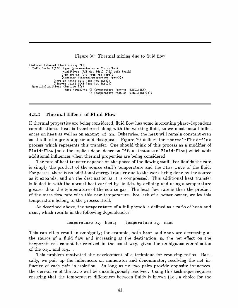
Figure 30 : Thermal mixing due to fluid flow

(defview (thermal-fluid-mixing ?ff)Individuals

((?ff

:type

(process-instance fluid-flow):conditions

(?ff dst ?dst)

(?ff path ?path)(?ff src-cs

(C-S ?sub ?st ?src))(Consider

(thermal-properties

?path)))(?src-cs

:bind (C-S ?sub ?st ?src))(?dst-cs

:bindQuantityConditions

((active(C-S?ff)

?sub ?st

?dst)))

(not (equal-to (A (temperature ?src-cs :ABSOLUTE))(A (temperature ?dst-cs :ABSOLUTE))))))

4 .3 .3 Thermal Effects of Fluid Flow

If thermal properties are being considered, fluid flow has some interesting phase-dependentcomplications. Heat is transferred along with the working fluid, so we must install influ-ences on heat as well as on amount-of-in . Otherwise, the heat will remain constant evenas the fluid objects appear and disappear . Figure 29 defines the thermal-fluid-flow

process which represents this transfer . One should think of this process as a modifier ofFluid-Flow (note the explicit dependence on ?ff, an instance of Fluid-Flow) which addsadditional influences when thermal properties are being considered.

The rate of heat transfer depends on the phase of the flowing stuff . For liquids the rateis simply the product of the source stuff's temperature and the flow-rate of the fluid.For gasses, there is an additional energy transfer due to the work being done by the sourceas it expands, and on the destination as it is compressed . This additional heat transferis folded in with the normal heat carried by liquids, by defining and using a temperaturegreater than the temperature of the source gas . The heat flow rate is then the productof the mass flow rate with this new temperature . For lack of a better owner, we let thistemperature belong to the process itself.

As described above, the temperature of a full physob is defined as a ratio of heat andmass, which results in the following dependencies:

temperature 0 Q+ heat ;

temperature aQ _ mass

This can often result in ambiguity ; for example, both heat and mass are decreasing atthe source of a fluid flow and increasing at the destination, so the net effect on thetemperatures cannot be resolved in the usual way, given the ambiguous combinationof the a Q + and o(Q_

This problem motivated the development of a technique for resolving ratios . Basi-cally, we pair up the influencers on numerator and denominator, resolving the net in-fluence of each pair in isolation. As long as no two pairs provide opposite influences,the derivative of the ratio will be unambiguously resolved . Using this technique requiresensuring that the temperature differences between fluids is known (i .e., a choice for the

41

relationship between temperatures is part of the constituents of a qualitative state) . TheThermal-Fluid-Mixing view of Figure 30 does this.

Augmented with this technique, QPE is powerful enough to reason that the temperature

at the source of a liquid flow remains constant, while the temperature at the destinationbehaves according to the difference in temperatures . This technique also solved anotherproblem: recognizing that flow into an empty container results in a contained-stuff at thesame temperature as the flow coming in . By requiring that a massless contained-stuff haveconstant temperature, it follows that the initial temperature will be the same as that ofthe liquid flowing in (otherwise it would be changing, a contradiction) . This constraintalso covers cases of multiple flows of different temperatures into an empty container.

4 .3 .4 Pumped Flow

Pumps are used to drive fluid flow when gravity won't . Pumps are modeled like paths:They don't have stuffs in them, but they move stuffs from place to place.

There are several design decisions concerning pump models . First, we must choose howto model a pump's flow rate . The simplest model of a pump assumes a constant (positive)flow rate, as long as there is fluid in the source container to be pumped . This modelcorresponds to a positive–displacement pump for liquids . Alternatively, we can model thepump's flow rate as a function of the pressure rise (or drop) across the pump . This modelis based on the (more common) centrifugal pump, in which the flow rate depends on thepressure rise (or drop) across the pump . The rate of flow decreases as the pressure riseincreases, until some maximum pressure is reached . We express our choice between thesealternatives with the Pumped-Flow-Variation assumption.

When considering Pumped-Flow-Variation, we may also wish to consider the pos-sibility that the pressure rise across the pump exceeds its maximum pumping pressure,causing a net flow in the reverse direction .14 This modeling choice is activated with thePump-Lossage consider assumption.

One possible behavior of pumps of general concern is cavitation, where the pressurechanges in a pump cause the liquid inside it to boil . We do not model cavitation in detail,except to note that it is likely to occur when pumping liquids that are already boiling.Such possibilities are detected only when the Pump-Cavitation assumption is in force.

The above modeling assumptions concern the actual operation of the pump . We mayalso wish to control whether or not we distinguish between different pump behaviors . Forexample, when a pump moves fluid from a lower to a higher pressure it is doing work, butwhen it is moving fluid from a higher pressure to a lower one, the pump is coasting . The(Consider Pump-Status) assumption causes this distinction to be made.

Details of the pump model The basic definitions for pumps is shown in Figure 31.These definitions parallel the definitions for fluid paths described in Section 4 .2 .4. A pumpmay be either a liquid-pump, a gas-pump, or both (e .g., a general-fluid-pump.

14This model of a pump is equivalent to a constant displacement pump in parallel with a (restricted) flowpath .

42

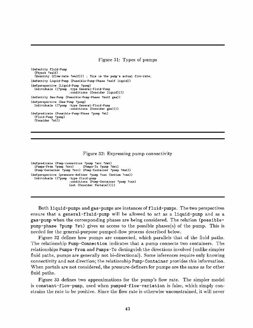
Figure 31 : Types of pumps

(defentity Fluid-Pump(Physob ?self)(Quantity (flow-rate ?self))) ; This is the pump's actual flow-rate;

(defentity Liquid-Pump (Possible-Pump-Phase ?self liquid))

(defperspective (Liquid-Pump ?pump)Individuals ((?pump type General-Fluid-Pump

conditions (Consider liquid))))

(defentity Gas-Pump (Possible-Pump-Phase ?self gas))

(defperspective (Gas-Pump ?pump)Individuals ((?pump type General-Fluid-Pump

conditions (Consider gas))))

(defpredicate (Possible-Pump-Phase ?pump ?st)(Fluid-Pump ?pump)(Consider ?st))

Figure 32 : Expressing pump connectivity

(defpredicate

(Pump-connection ?pump ?src ?dst)

?dst))(Pumps-From ?pump ?src)

(Pumps-To ?pump(Pump-Container ?pump ?src)

(Pump-Container?dst)?pump

(defperspective

(pressure-definer ?pump ?can (bottom ?can))Individuals ((?pump type fluid-pump

conditions (Pump-Container ?pump ?can)(not (Consider Portals)))))

Both liquid-pumps and gas-pumps are instances of fluid-pumps . The two perspectivesensure that a general-fluid-pump will be allowed to act as a liquid-pump and as agas-pump when the corresponding phases are being considered . The relation (possible-pump-phase ?pump ?st) gives us access to the possible phases(s) of the pump . This isneeded for the general-purpose pumped-flow process described below.

Figure 32 defines how pumps are connected, which parallels that of the fluid paths.The relationship Pump-Connection indicates that a pump connects two containers . Therelationships Pumps-From and Pumps-To distinguish the directions involved (unlike simplerfluid paths, pumps are generally not bi-directional) . Some inferences require only knowingconnectivity and not direction ; the relationship Pump-Container provides this information.When portals are not considered, the pressure-definers for pumps are the same as for otherfluid paths.

Figure 33 defines two approximations for the pump's flow rate . The simpler modelis constant-flow-pump, used when pumped-flow-variation is false, which simply con-strains the rate to be positive . Since the flow rate is otherwise unconstrained, it will never

43

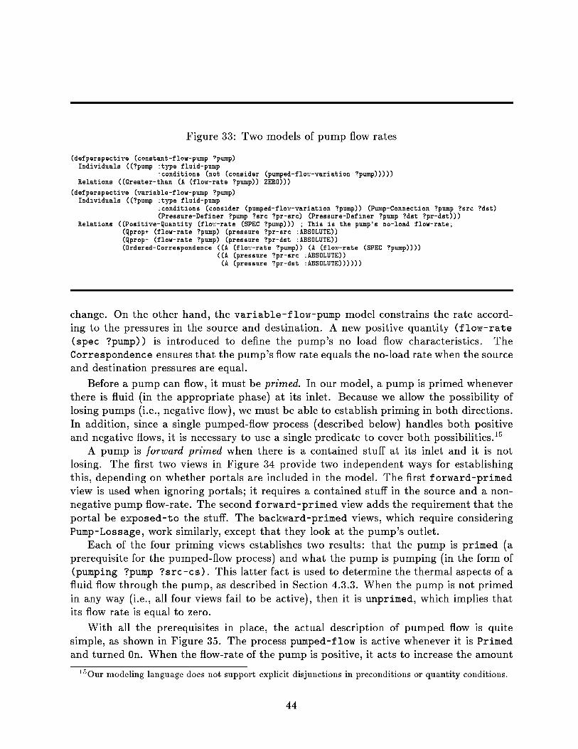
Figure 33 : Two models of pump flow rates

(defperspective (constant-flow-pump ?pump)Individuals ((?pump type fluid-pump

conditions (not (consider (pumped-flow-variation ?pump)))))Relations ((Greater-than (A (flow-rate ?pump)) ZERO)))

(defperspective (variable-flow-pump ?pump)Individuals ((?pump type fluid-pump

conditions (consider (pumped-flow-variation ?pump)) (Pump-Connection ?pump ?src ?dst)(Pressure-Definer ?pump ?src ?pr-src) (Pressure-Definer ?pump ?dst ?pr-dst)))

Relations ((Positive-Quantity (flow-rate (SPEC ?pump))) ; This is the pump's no-load flow-rate;(Qprop+ (flow-rate ?pump) (pressure ?pr-src :ABSOLUTE))(Qprop- (flow-rate ?pump) (pressure ?pr-dst :ABSOLUTE))(Ordered-Correspondence ((A (flow-rate ?pump)) (A (flow-rate (SPEC ?pump))))

((A (pressure ?pr-src :ABSOLUTE))(A (pressure ?pr-dst :ABSOLUTE))))))

change . On the other hand, the variable-flow-pump model constrains the rate accord-ing to the pressures in the source and destination. A new positive quantity (flow-rate

(spec ?pump)) is introduced to define the pump's no load flow characteristics . TheCorrespondence ensures that the pump's flow rate equals the no-load rate when the sourceand destination pressures are equal.

Before a pump can flow, it must be primed. In our model, a pump is primed wheneverthere is fluid (in the appropriate phase) at its inlet. Because we allow the possibility oflosing pumps (i .e., negative flow), we must be able to establish priming in both directions.In addition, since a single pumped-flow process (described below) handles both positiveand negative flows, it is necessary to use a single predicate to cover both possibilities . l5

A pump is forward primed when there is a contained stuff at its inlet and it is notlosing. The first two views in Figure 34 provide two independent ways for establishingthis, depending on whether portals are included in the model . The first forward-primed

view is used when ignoring portals ; it requires a contained stuff in the source and a non-negative pump flow-rate . The second forward-primed view adds the requirement that theportal be exposed-to the stuff. The backward-primed views, which require consideringPump-Lossage, work similarly, except that they look at the pump's outlet.

Each of the four priming views establishes two results : that the pump is primed (aprerequisite for the pumped-flow process) and what the pump is pumping (in the form of(pumping ?pump ?src-cs) . This latter fact is used to determine the thermal aspects of afluid flow through the pump, as described in Section 4 .3 .3. When the pump is not primedin any way (i .e., all four views fail to be active), then it is unprimed, which implies thatits flow rate is equal to zero.

With all the prerequisites in place, the actual description of pumped flow is quitesimple, as shown in Figure 35. The process pumped-flow is active whenever it is Primed

and turned On . When the flow-rate of the pump is positive, it acts to increase the amount

15Our modeling language does not support explicit disjunctions in preconditions or quantity conditions.

44

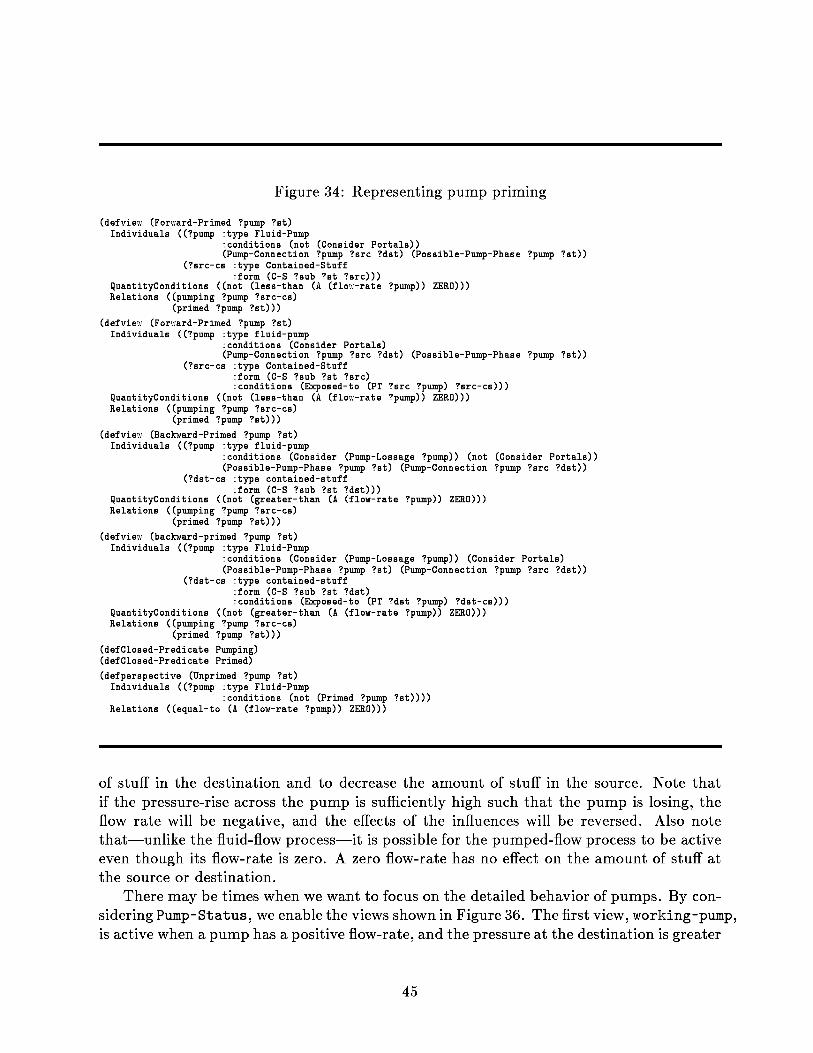
Figure 34: Representing pump priming

(defview (Forward-Primed ?pump ?st)Individuals ((?pump type Fluid-Pump

conditions (not (Consider Portals))(Pump-Connection ?pump ?src ?dst) (Possible-Pump-Phase ?pump ?st))

(?src-cs type Contained-Stuffform (C-S ?sub ?st ?src)))

QuantityConditions ((not (less-than (A (flow-rate ?pump)) ZERO)))Relations ((pumping ?pump ?src-cs)

(primed ?pump ?st)))

(defview (Forward-Primed ?pump ?st)Individuals ((?pump type fluid-pump

conditions (Consider Portals)(Pump-Connection ?pump ?src ?dst) (Possible-Pump-Phase ?pump ?st))

(?src-cs type Contained-Stuffform (C-S ?sub ?st ?src)conditions (Exposed-to (PT ?src ?pump) ?src-cs)))

QuantityConditions ((not (less-than (A (flow-rate ?pump)) ZERO)))Relations ((pumping ?pump ?src-cs)

(primed ?pump ?st)))

(defview (Backward-Primed ?pump ?st)Individuals ((?pump type fluid-pump

conditions (Consider (Pump-Lossage ?pump)) (not (Consider Portals))(Possible-Pump-Phase ?pump ?st) (Pump-Connection ?pump ?src ?dst))

(?dst-cs type contained-stuffform (C-S ?sub ?st ?dst)))

QuantityConditions ((not (greater-than (A (flow-rate ?pump)) ZERO)))Relations ((pumping ?pump ?src-cs)

(primed ?pump ?st)))

(defview (backward-primed ?pump ?st)Individuals ((?pump type Fluid-Pump

conditions (Consider (Pump-Lossage ?pump)) (Consider Portals)(Possible-Pump-Phase ?pump ?st) (Pump-Connection ?pump ?src ?dst))

(?dst-cs type contained-stuffform (C-S ?sub ?st ?dst)conditions (Exposed-to (PT ?dst ?pump) ?dst-cs)))

QuantityConditions ((not (greater-than (A (flow-rate ?pump)) ZERO)))Relations ((pumping ?pump ?src-cs)

(primed ?pump ?st)))

(defClosed-Predicate Pumping)(defClosed-Predicate Primed)

(defperspective (Unprimed ?pump ?st)Individuals ((?pump type Fluid-Pump

conditions (not (Primed ?pump ?st))))Relations ((equal-to (A (flow-rate ?pump)) ZERO)))

of stuff in the destination and to decrease the amount of stuff in the source . Note that

if the pressure-rise across the pump is sufficiently high such that the pump is losing, the

flow rate will be negative, and the effects of the influences will be reversed . Also note

that—unlike the fluid-flow process—it is possible for the pumped-flow process to be active

even though its flow-rate is zero . A zero flow-rate has no effect on the amount of stuff at

the source or destination.

There may be times when we want to focus on the detailed behavior of pumps . By con-

sidering Pump-Status, we enable the views shown in Figure 36 . The first view, working-pump,

is active when a pump has a positive flow-rate, and the pressure at the destination is greater

45

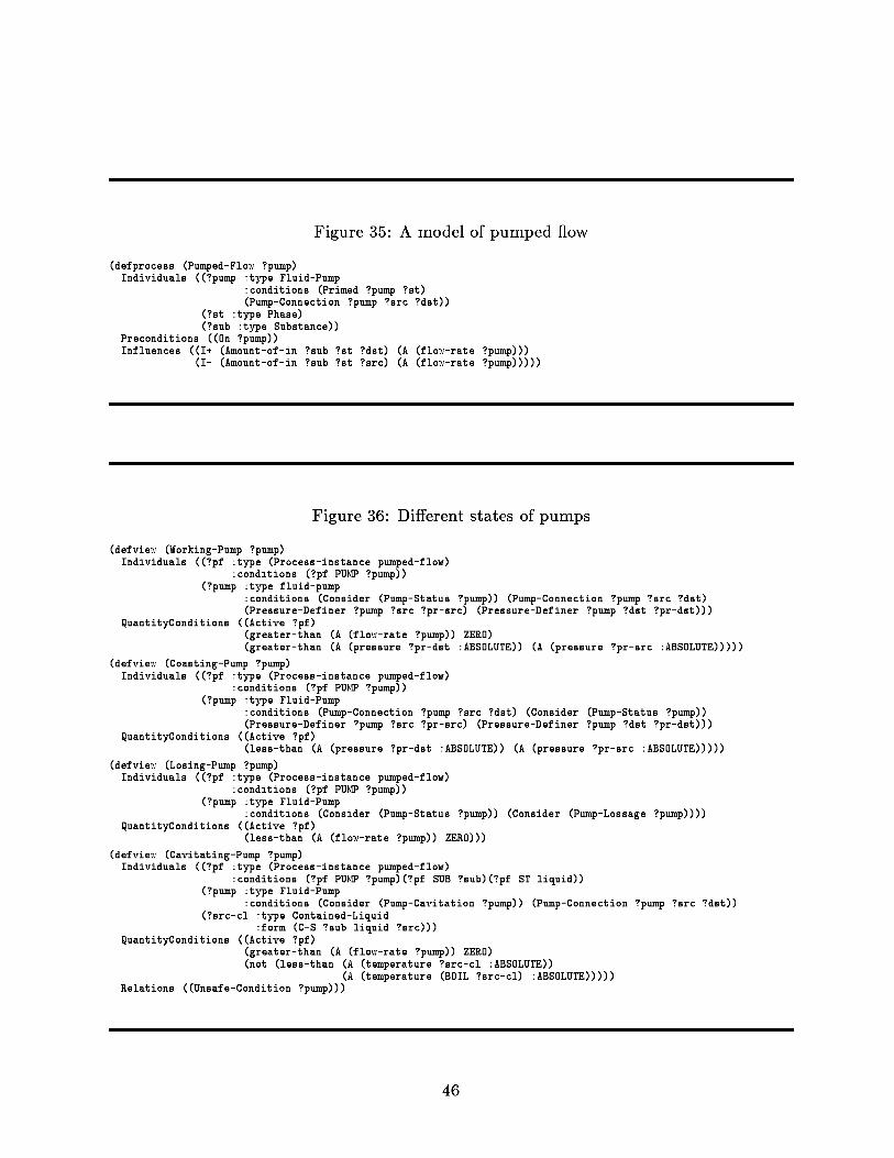
Figure 35 : A model of pumped flow

(defprocess (Pumped-Flow ?pump)Individuals ((?pump type Fluid-Pump

conditions (Primed ?pump ?st)(Pump-Connection ?pump ?src ?dst))

(?st type Phase)(?sub :type Substance))

Preconditions ((On ?pump))Influences ((I+ (Amount-of-in ?sub ?st ?dst) (A (flow-rate ?pump)))

(I- (Amount-of-in ?sub ?st ?src) (A (flow-rate ?pump)))))

Figure 36 : Different states of pumps

(defview (Working-Pump ?pump)Individuals ((?pf type (Process-instance pumped-flow)

conditions (?pf PUMP ?pump))(?pump type fluid-pump

conditions (Consider (Pump-Status ?pump)) (Pump-Connection ?pump ?src ?dst)(Pressure-Definer ?pump ?src ?pr-src) (Pressure-Definer ?pump ?dst ?pr-dst)))

QuantityConditions ((Active ?pf)(greater-than (A (flow-rate ?pump)) ZERO)(greater-than (A (pressure ?pr-dst :ABSOLUTE)) (A (pressure ?pr-src :ABSOLUTE)))))

(defview (Coasting-Pump ?pump)Individuals ((?pf type (Process-instance pumped-flow)

conditions (?pf PUMP ?pump))(?pump type Fluid-Pump

conditions (Pump-Connection ?pump ?src ?dst) (Consider (Pump-Status ?pump))(Pressure-Definer ?pump ?src ?pr-src) (Pressure-Definer ?pump ?dst ?pr-dst)))

QuantityConditions ((Active ?pf)(less-than (A (pressure ?pr-dst :ABSOLUTE)) (A (pressure ?pr-src :ABSOLUTE)))))

(defview (Losing-Pump ?pump)Individuals ((?pf type (Process-instance pumped-flow)

conditions (?pf PUMP ?pump))(?pump type Fluid-Pump

conditions (Consider (Pump-Status ?pump)) (Consider (Pump-Lossage ?pump))))QuantityConditions ((Active ?pf)

(less-than (A (flow-rate ?pump)) ZERO)))

(defview (Cavitating-Pump ?pump)Individuals ((?pf type (Process-instance pumped-flow)

conditions (?pf PUMP ?pump)(?pf SUB ?sub)(?pf ST liquid))(?pump type Fluid-Pump

conditions (Consider (Pump-Cavitation ?pump)) (Pump-Connection ?pump ?src ?dst))(?src-cl :type Contained-Liquid

:form (C-S ?sub liquid ?src)))QuantityConditions ((Active ?pf)

(greater-than (A (flow-rate ?pump)) ZERO)(not (less-than (A (temperature ?src-cl :ABSOLUTE))

(A (temperature (BOIL ?src-cl) :ABSOLUTE)))))Relations ((Unsafe-Condition ?pump)))

46

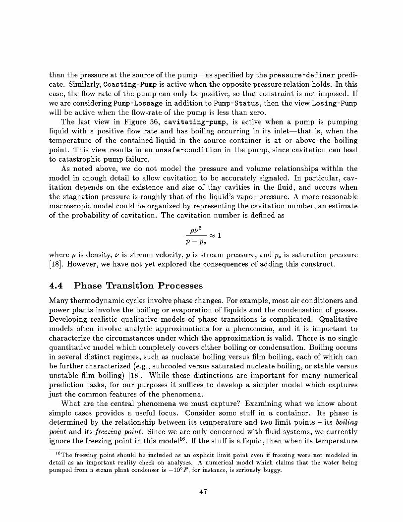
than the pressure at the source of the pump—as specified by the pressure-definer predi-

cate. Similarly, Coasting-Pump is active when the opposite pressure relation holds . In this

case, the flow rate of the pump can only be positive, so that constraint is not imposed . If

we are considering Pump-Lossage in addition to Pump-Status, then the view Losing-Pump

will be active when the flow-rate of the pump is less than zero.

The last view in Figure 36, cavitating-pump, is active when a pump is pumping

liquid with a positive flow rate and has boiling occurring in its inlet—that is, when the

temperature of the contained-liquid in the source container is at or above the boiling

point. This view results in an unsafe-condition in the pump, since cavitation can lead

to catastrophic pump failure.

As noted above, we do not model the pressure and volume relationships within the

model in enough detail to allow cavitation to be accurately signaled . In particular, cav-

itation depends on the existence and size of tiny cavities in the fluid, and occurs when

the stagnation pressure is roughly that of the liquid's vapor pressure . A more reasonable

macroscopic model could be organized by representing the cavitation number, an estimate

of the probability of cavitation . The cavitation number is defined as

pv2

--P

where p is density, v is stream velocity, p is stream pressure, and ps is saturation pressure

[18] . However, we have not yet explored the consequences of adding this construct.

4 .4 Phase Transition Processes

Many thermodynamic cycles involve phase changes . For example, most air conditioners and

power plants involve the boiling or evaporation of liquids and the condensation of gasses.

Developing realistic qualitative models of phase transitions is complicated . Qualitative

models often involve analytic approximations for a phenomena, and it is important to

characterize the circumstances under which the approximation is valid . There is no single

quantitative model which completely covers either boiling or condensation . Boiling occurs

in several distinct regimes, such as nucleate boiling versus film boiling, each of which can

be further characterized (e .g ., subcooled versus saturated nucleate boiling, or stable versus

unstable film boiling) [18] . While these distinctions are important for many numerical

prediction tasks, for our purposes it suffices to develop a simpler model which captures

just the common features of the phenomena.

What are the central phenomena we must capture? Examining what we know about

simple cases provides a useful focus . Consider some stuff in a container . Its phase is

determined by the relationship between its temperature and two limit points - its boilingpoint and its freezing point . Since we are only concerned with fluid systems, we currently

ignore the freezing point in this model16 . If the stuff is a liquid, then when its temperature

16The freezing point should be included as an explicit limit point even if freezing were not modeled indetail as an important reality check on analyses . A numerical model which claims that the water beingpumped from a steam plant condenser is -10°F, for instance, is seriously buggy.

47

rises to the boiling point boiling occurs . When it is a gas and its temperature drops to theboiling point condensation occurs.

We now know what processes we must model and something about the conditionsunder which they occur . What else must we know? An important fact is that the boilingpoint of a substance is not constant but increases with pressure . For example, boiling(and condensation) occur at a higher temperature in a pressurized vessel (such as a car'sradiator or a pressure cooker) than in an open pan on a stove. Likewise, lukewarm waterwill boil in a vacuum, and superheated steam will condense when subjected to sufficientlyhigh pressure. A qualitative proportionality suffices to model this fact . But where in themodel should it be installed? If we were always considering phase changes, the naturalplace to include this fact is in the Complex-Physob description . By now the alert readersuspects that a more subtle representation is used instead, and this suspicion is correct.

Boiling and condensation are in nearly all respects symmetric processes, so we referprimarily to boiling in our discussion of phase transitions and describe condensation byhighlighting the few ways in which it is different.

4 .4 .1 Thermal Behavior of Phase Transitions

Having a temperature equal to its boiling point is not sufficient for a liquid to boil —heat must be continually added to carry out the phase transformation . Since the internalenergy of the contained liquid does not rise, its temperature remains roughly constantduring boiling . If the heat flow is halted, boiling stops almost immediately . The amountof heat required to boil a unit measure of liquid, once it is heated to its boiling point, isknown as the latent heat of vaporization.

Although our model of boiling is in terms of qualitative equations relating continuousparameters, to justify the model it is useful to conceptually decompose the boiling processinto an equivalent sequence of simple events . For example, boiling may be decomposed inthe following way:

1. An infinitesimal piece of liquid is selected as the next candidate to undergo thetransition from liquid to gas . This infinitesimal piece of liquid is removed from thecontained-liquid by subtracting out its mass and heat content from the correspondingproperties of the contained-liquid.

2. To convert the piece of liquid into a piece of gas, additional heat corresponding toits latent heat of vaporization is transferred to the piece of liquid.

3. As the phase transition proceeds, the piece-of-stuff expands, thereby expending en-ergy (heat) as it does work on its surrounding contained-gas.

4. Finally, the piece of gas is added to the contained-gas by incrementing its mass, heatand volume.

Notice that the internal energy of the stuff is conserved . Where does the latent heatof vaporization come from? There are several options . First, we could require an external

48

heat source, whose temperature is above the boiling point . The rate of boiling is thenqualitatively proportional to the heat flow rate into the liquid.

This model captures several of our important intuitions about boiling, but has certainlimitations . One problem concerns multiple heat flows into and out of the liquid . Thismodel of boiling requires a net positive flow of heat into the liquid, but our model doesnot currently provide such a quantity 17 . Even if this quantity were available, it would beincorrect to define the boiling rate solely in terms of the net heat flow . In fact one can boila liquid without adding any heat at all, simply by reducing the pressure and thus reducingthe boiling point below the current temperature of the liquid.

This leads to the second model : Allow the latent heat of vaporization to flow from theboiling liquid itself . This model captures vaccum boiling, but introduces a new problem —what determines the rate at which it proceeds? There is no net heat flow rate to constrainit, unlike the first model. An analogy with liquid overflow suggests an answer . In liquidoverflow, the idea that the level of the liquid was never higher than the top of the containeris seen as an idealization. The reality is that for overflow to occur, the level must exceedthe top height of the container, and the height difference determines the rate of overflow.Similarly, we can consider the rate of boiling to be qualitatively proportional to the degreeto which the liquid's temperature exceeds its boiling temperature, if we realize that, likeoverflow, the temperature of a boiling liquid equalling its boiling point is actually anidealization.

At first this model may seem somewhat unintuitive . But, if you consider what happenswhen you remove the air from a flask containing water, you will notice that the boilingoccurs faster when the flask pressure is lower (i .e., when the boiling point/temperaturedifference is greater) . Thinking about a piece-of-stuff perspective provides further support.A boiling liquid does not actually have a single temperature ; rather it has a distribution oftemperatures which has some particular mean that we call "the" temperature . Droppingto the molecular level, this means some molecules will be moving faster than others . Ifwe view the boiling process as Maxwell's demon grabbing and removing only the fastestmolecules, then clearly the average temperature of the liquid is reduced as a result.

The first model may be viewed as a time-scale abstraction ([14]) of the second model,just as our fluid flow model abstracts away any inertial effects of the fluid in the path . Onedrawback of the second model is that it allows boiling to occur even when there is no heatflow into the liquid and the boiling point is constant . While this phenomenon may actuallyoccur, it is of such short duration that we would prefer not to include it in our model.The removal of latent heat from a boiling liquid should be sufficiently high to prevent theliquid from heating up more than infinitesimally above the boiling point . Without orderof magnitude reasoning, however, we have no way to express this constraint.

Each of these models for boiling provides different advantages, so the domain modelincludes them both . The second model is predicated on the assumption (Consider

17The current QPE modeling language does not implement a primitive for taking sums over explicit domain-specific sets, which is necessary to define a net-heat-flow parameter . Overcoming this limitation appearsto be straightforward, but we have not had time to implement it yet.

49

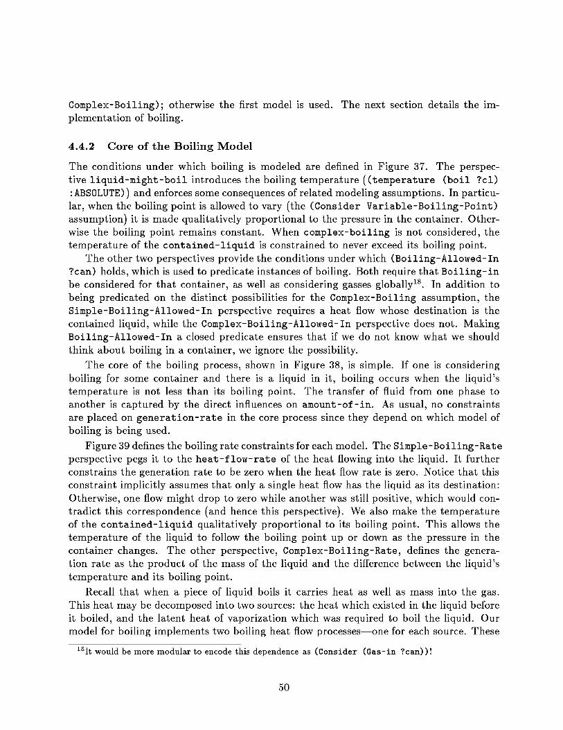
Complex-Boiling) ; otherwise the first model is used . The next section details the im-plementation of boiling.

4 .4 .2 Core of the Boiling Model

The conditions under which boiling is modeled are defined in Figure 37 . The perspec-tive liquid-might-boil introduces the boiling temperature ((temperature (boil ?cl): ABSOLUTE)) and enforces some consequences of related modeling assumptions . In particu-lar, when the boiling point is allowed to vary (the (Consider Variable-Boiling-Point)assumption) it is made qualitatively proportional to the pressure in the container . Other-wise the boiling point remains constant . When complex-boiling is not considered, thetemperature of the contained-liquid is constrained to never exceed its boiling point.

The other two perspectives provide the conditions under which (Boiling-Allowed-In

?can) holds, which is used to predicate instances of boiling . Both require that Boiling-inbe considered for that container, as well as considering gasses globally 18 . In addition tobeing predicated on the distinct possibilities for the Complex-Boiling assumption, theSimple-Boiling-Allowed-In perspective requires a heat flow whose destination is thecontained liquid, while the Complex-Boiling-Allowed-In perspective does not . MakingBoiling-Allowed-In a closed predicate ensures that if we do not know what we shouldthink about boiling in a container, we ignore the possibility.

The core of the boiling process, shown in Figure 38, is simple . If one is consideringboiling for some container and there is a liquid in it, boiling occurs when the liquid'stemperature is not less than its boiling point. The transfer of fluid from one phase toanother is captured by the direct influences on amount-of-in . As usual, no constraintsare placed on generation-rate in the core process since they depend on which model ofboiling is being used.

Figure 39 defines the boiling rate constraints for each model . The Simple-Boiling-Rateperspective pegs it to the heat-flow-rate of the heat flowing into the liquid . It furtherconstrains the generation rate to be zero when the heat flow rate is zero . Notice that thisconstraint implicitly assumes that only a single heat flow has the liquid as its destination:Otherwise, one flow might drop to zero while another was still positive, which would con-tradict this correspondence (and hence this perspective) . We also make the temperatureof the contained-liquid qualitatively proportional to its boiling point . This allows thetemperature of the liquid to follow the boiling point up or down as the pressure in thecontainer changes . The other perspective, Complex-Boiling-Rate, defines the genera-tion rate as the product of the mass of the liquid and the difference between the liquid'stemperature and its boiling point.

Recall that when a piece of liquid boils it carries heat as well as mass into the gas.This heat may be decomposed into two sources : the heat which existed in the liquid beforeit boiled, and the latent heat of vaporization which was required to boil the liquid . Ourmodel for boiling implements two boiling heat flow processes—one for each source . These

18It would be more modular to encode this dependence as (Consider (Gas-in ?can))!

50

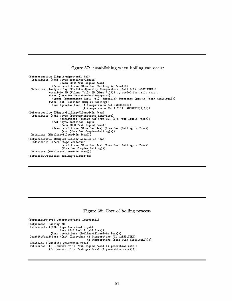
Figure 37: Establishing when boiling can occur

(defperspective (liquid-might-boil ?cl)Individuals ((?cl type contained-liquid

form (C-S ?sub liquid ?can))(?can conditions (Consider (Boiling-in ?can))))

Relations ((only-during (Positive-Quantity (temperature (Boil ?cl) :ABSOLUTE)))(equal-to (D (Volume ?cl)) (D (Mass ?cl))) ; ; needed for ratio code . ..(When (Consider Variable-boiling-point)(Qprop (temperature (Boil ?cl) :ABSOLUTE) (pressure (gas-in ?can) :ABSOLUTE)))

(When (not (Consider Complex-Boiling))(not (greater-than (A (temperature ?cl :ABSOLUTE))

(A (temperature (boil ?cl) :ABSOLUTE)))))))

(defperspective (Simple-Boiling-Allowed-In ?can)Individuals ((?hf type (process-instance heat-flow)

conditions (active ?hf)(?hf DST (C-S ?sub liquid ?can)))(?cl type contained-liquid

form (C-S ?sub liquid ?can))(?can conditions (Consider Gas) (Consider (Boiling-in ?can))

(not (Consider Complex-Boiling))))Relations ((Boiling-Allowed-In ?can)))

(defperspective (Complex-Boiling-Allowed-In ?can)Individuals ((?can type container

conditions (Consider Gas) (Consider (Boiling-in ?can))(Consider Complex-Boiling)))

Relations ((Boiling-Allowed-In ?can)))

(defClosed-Predicate Boiling-Allowed-In)

Figure 38 : Core of boiling process

(defQuantity-Type Generation-Rate Individual)

(defprocess (Boiling ?CL)Individuals ((?CL :type Contained-Liquid

:form (C-S ?sub liquid ?can))(?can conditions (Boiling-Allowed-in ?can)))

QuantityConditions ((not (less-than (A (temperature ?CL :ABSOLUTE))(A (temperature (boil ?CL) :ABSOLUTE)))))

Relations ((Quantity generation-rate))Influences ((I- (amount-of-in ?sub liquid ?can) (A generation-rate))

(I+ (amount-of-in ?sub gas ?can) (A generation-rate))))

51

Figure 39: Defining the rate of the boiling process

(defperspective (Simple-Boiling-Rate ?bp ?hf)Individuals ((?bp :type (Process-Instance Boiling)

:conditions (Active ?bp) (?bp CL ?cl)(not (Consider Complex-Boiling)))

(?hf :type (Process-Instance Heat-Flow):conditions (Active ?hf) (?hf DST ?cl)))

Relations ((Qprop (generation-rate ?bp) (heat-flow-rate ?hf))Assumes there will only be one of these!!

(Ordered-Correspondence ((A (generation-rate ?bp)) ZERO)((A (heat-flow-rate ?hf)) ZERO))

; Keep it boiling in a rising pressure:(Qprop (temperature ?CL :ABSOLUTE) (temperature (boil ?CL) :ABSOLUTE))))

(defperspective (complex-boiling-rate ?bp)Individuals ((?bp :type (process-instance boiling)

:conditions (active ?bp)(?bp CL ?cl)(Consider Complex-Boiling)))

Relations ((Quantity (temperature ?cl (boil ?cl)))(Q= (temperature ?cl (boil ?cl))

(- (temperature ?cl :ABSOLUTE)(temperature (boil ?cl) :ABSOLUTE)))

(Q= (Generation-Rate ?bp)(*0+ (temperature ?cl (boil ?cl)) (mass ?CL)))))

are given in Figure 40 . The boiling-heat-flow process accounts for the heat transfer due

to the transfer of fluid from the liquid to the gas . This process will only be active when

we are considering Thermal-Boiling . The heat-flow-rate of the process is defined as

the product of the generation-rate of the boiling process times the temperature of the

boiling liquid . This influence on heat—together with the influence of the generation-rate

on mass—will result in a zero net influence on the temperature of the liquid.

The latent heat of vaporization must be added to a piece of liquid as it boils, and

is assumed to flow from the contained-liquid to the contained-gas . The second process in

Figure 40 implements this flow of latent heat of vaporization. Boiling-Latent-Heat-Flow

is active when we are considering latent-heat-of-vaporization, and provides a second

influence on the heat of the liquid and the gas . The heat-flow-rate of this process is

made qualitatively equal to the generation-rate of the boiling process.

Recall that for the simple model of boiling, the generation-rate is equal to the

heat-flow-rate of the heat-flow process which is driving the boiling . Thus for sim-

ple boiling, these two influences on the heat of the liquid cancel each other, leaving

only the influence of the boiling-heat-flow process described above . In the case of

complex-boiling, the heat of the contained-liquid is negatively influenced both by the

removal of liquid and by the drain caused by the latent heat of vaporization, so the net

influence on the liquid's temperature is negative. This provides a stabilizing influence on

the boiling liquid by pushing its temperature back below the boiling point.

52

Figure 40 : Thermal effects of boiling

(defprocess (boiling-heat-flow ?bp)Individuals ((?bp type (process-instance boiling)

conditions (active ?bp)(?bp CL (C-S ?sub liquid ?can))(Consider thermal-boiling))

(?cl type Contained-Liquidform (C-S ?sub liquid ?can))

(?cg bind (C-S ?sub gas ?can)))Relations ((Quantity Heat-Flow-Rate)

(Q= Heat-Flow-Rate (*0+ (Generation-Rate ?bp)(temperature ?cl :ABSOLUTE))))

Influences ((I- (heat ?cl) (A Heat-Flow-Rate))(I+ (heat ?cg) (A Heat-Flow-Rate))))

(defprocess (boiling-latent-heat-flow ?bp)Individuals ((?bp type (process-instance boiling)

conditions (active ?bp)(?bp CL (C-S ?sub liquid ?can))(Consider latent-heat-of-vaporization))

(?cl type Contained-Liquidform (C-S ?sub liquid ?can))

(?cg bind (C-S ?sub gas ?can)))Relations ((Quantity Heat-Flow-Rate)

(Q= Heat-Flow-Rate (Generation-Rate ?bp)))Influences ((I- (heat ?cl) (A Heat-Flow-Rate))

(I+ (heat ?cg) (A Heat-Flow-Rate))))

4 .4 .3 Condensation

Condensation is defined by direct analogy with boiling . There is condensing process fora contained gas whose temperature is at or below the boiling point . When the process isactive it has a generation-rate which acts to decrease the amount of gas and to increasethe amount of liquid in the container . As with boiling, the rate is defined differentlydepending on whether one considers complex versus simple condensing . We actually usethe same consider assumption (Complex-Boiling) to ensure that we treat phase changessymmetrically.

Figure 41 defines three perspectives which together establish whether condensing isallowed in a particular container . These are exactly analogous to the perspectives in Figure37, but involving Condensing-In instead of Boiling-In . Similarly, Figure 42 describesthe core Condensing process, Figure 43 defines the constraints on the rate of condensation(i .e., the generation-rate, this time of liquid instead of gas), and Figure 44 defines thethermal effects of condensing.

The astute reader will notice a slight asymmetry between the models for boiling andcondensation : the condensation model does not refer to the latent heat of vaporization . Theassumption is that the latent heat of vaporization is always exchanged with the surroundingstuff—i.e ., the boiling liquid or the condensing gas . Since the condensing piece of gasdischarges its latent heat before becoming a part of the liquid condensate, the latent heatdoes not show up in the model for condensation . The two processes would be completelysymmetric if we assumed that the liquid condensate received the latent heat, but the

53

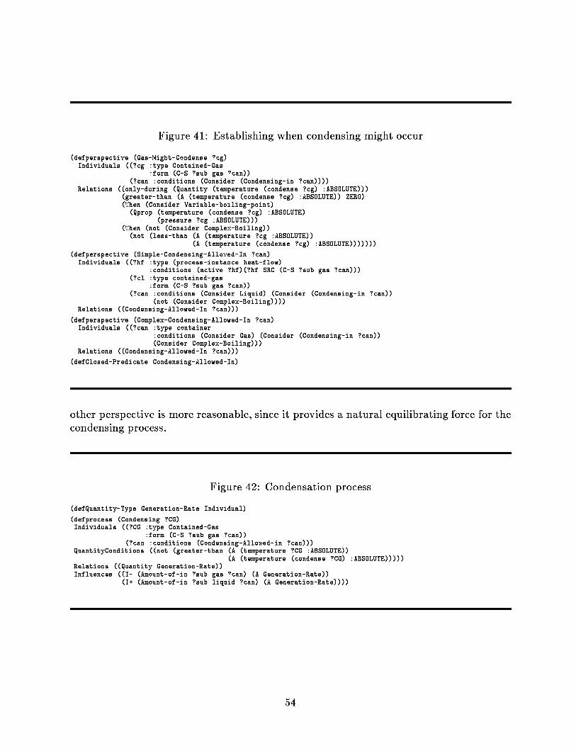
Figure 41 : Establishing when condensing might occur

(defperspective (Gas-Might-Condense ?cg)Individuals ((?cg type Contained-Gas

form (C-S ?sub gas ?can))(?can conditions (Consider (Condensing-in ?can))))

Relations ((only-during (Quantity (temperature (condense ?cg) :ABSOLUTE)))(greater-than (A (temperature (condense ?cg) :ABSOLUTE)) ZERO)(When (Consider Variable-boiling-point)(Qprop (temperature (condense ?cg) :ABSOLUTE)

(pressure ?cg :ABSOLUTE)))(When (not (Consider Complex-Boiling))(not (less-than (A (temperature ?cg :ABSOLUTE))

(A (temperature (condense ?cg) :ABSOLUTE)))))))

(defperspective (Simple-Condensing-Allowed-In ?can)Individuals ((?hf type (process-instance heat-flow)

conditions (active ?hf)(?hf SRC (C-S ?sub gas ?can)))(?cl type contained-gas

form (C-S ?sub gas ?can))(?can conditions (Consider Liquid) (Consider (Condensing-in ?can))

(not (Consider Complex-Boiling))))Relations ((Condensing-Allowed-In ?can)))

(defperspective (Complex-Condensing-Allowed-In ?can)Individuals ((?can type container

conditions (Consider Gas) (Consider (Condensing-in ?can))(Consider Complex-Boiling)))

Relations ((Condensing-Allowed-In ?can)))

(defClosed-Predicate Condensing-Allowed-In)

other perspective is more reasonable, since it provides a natural equilibrating force for the

condensing process .

Figure 42 : Condensation process

(defQuantity-Type Generation-Rate Individual)

(defprocess (Condensing ?CG)Individuals ((?CG :type Contained-Gas

:form (C-S ?sub gas ?can))(?can conditions (Condensing-Allowed-in ?can)))

QuantityConditions ((not (greater-than (A (temperature ?CG :ABSOLUTE))(A (temperature (condense ?CG) :ABSOLUTE)))))

Relations ((Quantity Generation-Rate))Influences ((I- (Amount-of-in ?sub gas ?can) (A Generation-Rate))

(I+ (Amount-of-in ?sub liquid ?can) (A Generation-Rate))))

54

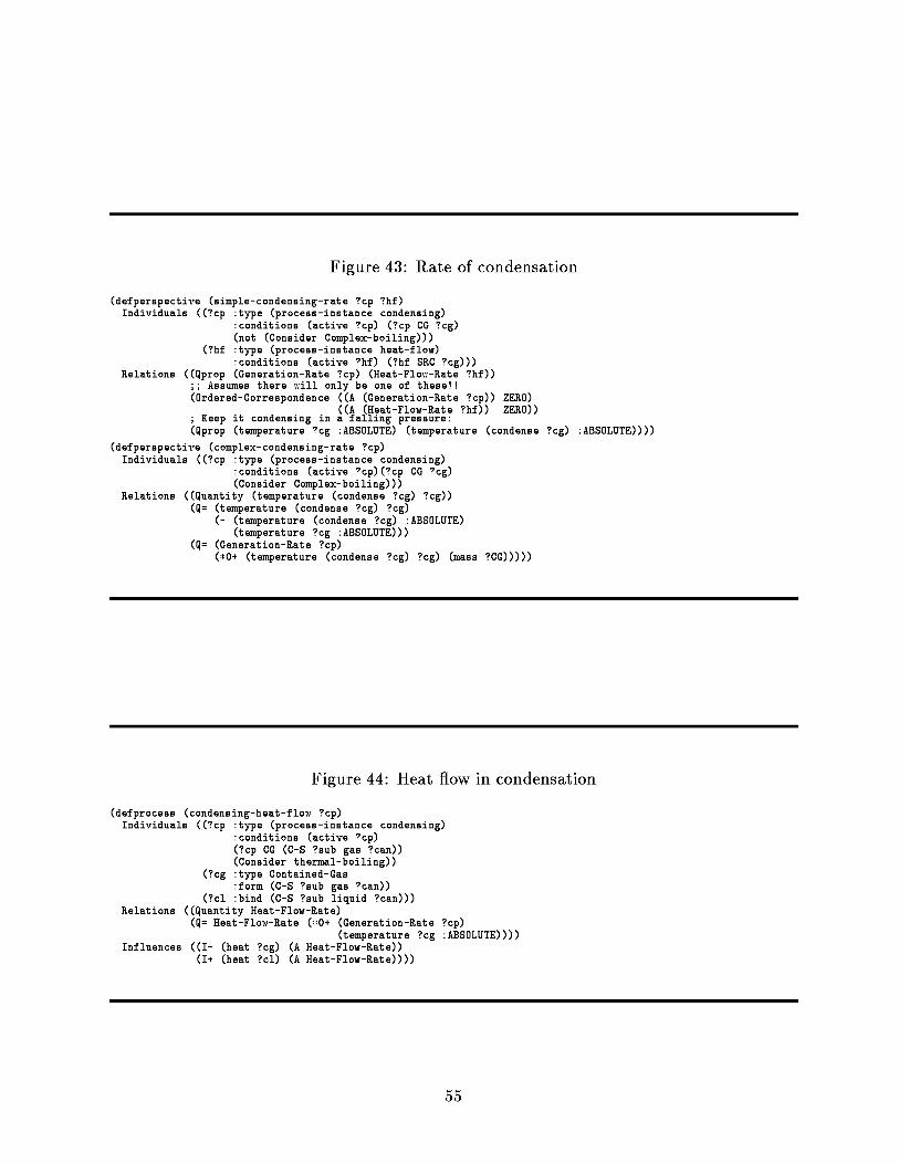
Figure 43: Rate of condensation

(defperspective (simple-condensing-rate ?cp ?hf)Individuals ((?cp :type (process-instance condensing)

:conditions (active ?cp) (?cp CG ?cg)(not (Consider Complex-boiling)))

(?hf :type (process-instance heat-flow):conditions (active ?hf) (?hf SRC ?cg)))

Relations ((Qprop (Generation-Rate ?cp) (Heat-Flow-Rate ?hf))Assumes there will only be one of these!!

(Ordered-Correspondence ((A (Generation-Rate ?cp)) ZERO)((A (Heat-Flow-Rate ?hf)) ZERO))

; Keep it condensing in a falling pressure:(Qprop (temperature ?cg :ABSOLUTE) (temperature (condense ?cg) :ABSOLUTE))))

(defperspective (complex-condensing-rate ?cp)Individuals ((?cp :type (process-instance condensing)

:conditions (active ?cp)(?cp CG ?cg)(Consider Complex-boiling)))

Relations ((Quantity (temperature (condense ?cg) ?cg))(Q= (temperature (condense ?cg) ?cg)

(- (temperature (condense ?cg) :ABSOLUTE)(temperature ?cg :ABSOLUTE)))

(Q= (Generation-Rate ?cp)(*0+ (temperature (condense ?cg) ?cg) (mass ?CG)))))

Figure 44 : Heat flow in condensation

(defprocess (condensing-heat-flow ?cp)Individuals ((?cp :type (process-instance condensing)

:conditions (active ?cp)(?cp CG (C-S ?sub gas ?can))(Consider thermal-boiling))

(?cg :type Contained-Gas:form (C-S ?sub gas ?can))

(?cl :bind (C-S ?sub liquid ?can)))Relations ((Quantity Heat-Flow-Rate)

(Q= Heat-Flow-Rate (*0+ (Generation-Rate ?cp)(temperature ?cg :ABSOLUTE))))

Influences ((I- (heat ?cg) (A Heat-Flow-Rate))(I+ (heat ?cl) (A Heat-Flow-Rate))))

55

Figure 45 : The logic of steady-state

(defperspective (Steady-State-Quantity ?qty)Individuals ((?qty type Quantity

conditions (Consider Steady-State))))

(defperspective (Steady-State-Quantity (?qty-type ?ind . ?rest))Individuals ((?ind conditions (Consider (Steady-State-Individual ?ind)))

(?qty-type :conditions (Quantity (?qty-type ?ind . ?rest)))))

(defperspective (Steady-State-Quantity (?qty-type . ?inds))Individuals ((?qty-type :conditions (Consider (Steady-State-Quantity-Type ?qty-type))

(Quantity (?qty-type . ?inds)))))

(defperspective (Steady-State-Quantity ?qty)Individuals ((?qty type Quantity

conditions (Consider (Steady-State-Quantity ?qty)))))

(defpredicate Steady-State-Quantity(Equal-to (D ?self) ZERO))

4 .5 Controlling the Model

4 .5 .1 Representing and enforcing the steady-state assumption

As models and scenarios become increasingly complex, it becomes more costly to generatetotal envisionments (e .g., all possible behaviors) . Often one is only interested in a particular behavior or class of behaviors . One common simplifying assumption in engineeringproblem solving is the steady state assumption . That is, all state variables have achievedan equilibrium, and whatever is happening in the system is occurring continuously, withouttransitions . This section introduces a variety of steady state assumptions, ranging in scopefrom a single quantity to an entire system.

Figure 45 shows how several different levels of assumptions about steady-state can beencoded uniformly. In all cases, the predicate Steady-State-Quantity is used to enforcethe result of these assumptions, pinning the derivative of the quantity to zero . The fourperspectives each correspond to a different level of specificity. The first triggers on theglobal assumption Steady-State, and the second triggers on assuming steady-state for aparticular individual. The third enforces steady-state on particular classes of quantities,while the fourth enforces it for a particular, given quantity.

4 .5 .2 Representing Nominal Values

Monitoring a system often involves tracking whether or not certain parameters arewithin specific tolerances . Figure 46 defines a simple model of tolerances . The modelingassumption (Tolerances ?qty) indicates that the tolerances on quantity ?qty should bemonitored. The Bounded perspective introduces two new quantities which serve as theupper and lower bounds (i .e., the lower-limit and upper-limit of ?qty) . Notice that,with the exception of the obvious constraint that the upper limit is greater than the lowerlimit, we have not constrained these limits at all . Typically, a model for a specific scenario

56

Figure 46 : Representing tolerances(defQuantity-Type lower-limit individual)(defQuantity-Type upper-limit individual)

(defperspective (Bounded ?qty)Individuals ((?qty type Quantity

conditions (Consider (Tolerances ?qty))))Relations ((Quantity (lower-limit ?qty))

(Quantity (upper-limit ?qty))(greater-than (A (upper-limit ?qty)) (A (lower-limit ?qty)))))

(defview (Under-Tolerance ?qty)Individuals ((?qty type Quantity

conditions (Consider (Tolerances ?qty))))QuantityConditions ((less-than (A ?qty) (A (Lower-Limit ?qty))))Relations ((Alarm (Under-Tolerance ?qty))))

(defview (Over-Tolerance ?qty)Individuals ((?qty type Quantity

conditions (Consider (Tolerances ?qty))))QuantityConditions ((greater-than (A ?qty) (A (Upper-Limit ?qty))))Relations ((Alarm (Over-Tolerance ?qty))))

would include extra inequalities to tie this generic concept to something more specific (i .e .,+10%) . The views Under-Tolerance and Over-Tolerance make these quantities intolimit points by relying on them as quantity conditions . As usual, this means that stateswill be distinguished according to whether or not a parameter is over, under, or within itstolerances . We further stipulate that the relation Alarm indicates the existence of some"interesting" condition . By including Alarm statements in the Relations field, we indicateexplicitly what quantities are out of tolerance in a state.

4 .5 .3 Enforcing Relationships Between Modeling Assumptions

The previous sections used modeling assumptions to allow alternate model fragments topeacefully coexist . This section discusses how relationships between modeling assumptionsare enforced, which of course is essential to ensuring that only coherent scenario modelsare constructed. These relationships take two forms . First, global assumptions aboutproperties of a system entail choices for assumptions about the parts of that system.Second, certain combinations of modeling assumptions are mutually incompatible . Wedescribe each kind in turn.

We must distinguish two types of modeling assumptions : global assumptions and local

assumptions . Global assumptions apply universally to the entire scenario 19 , while localassumptions refer to a particular object or subpart of the system. The entailments ofglobal modeling assumptions can be captured in part by propagation . For example, whenglobally considering Geometric-Properties, we want them to be locally considered forevery Container . We express this by asserting:

19In [4] global assumptions are represented as predicates on the distinguished symbol : SCENARIO, ratherthan as abstract tokens . We plan to convert the FSThermo model to this convention soon.

57

Figure 47: Inheriting modeling assumptions

(defperspective (Globally-Consider ?cnsdr ?type ?obj)Individuals ((?cnsdr :conditions (Propagate-Consideration ?cnsdr ?type) (Consider ?cnsdr))

(?obj :type ?type))Relations ((Consider (?cnsdr ?obj))))

(defperspective (Never-Consider ?cnsdr ?type ?obj)Individuals ((?cnsdr :conditions (Propagate-Consideration ?cnsdr ?type) (not (Consider ?cnsdr)))

(?obj

:type ?type))Relations

((not

(Consider

(?cnsdr

?obj)))))

Containers:(assertq (Propagate-Consideration Geometric-Properties Container))(assertq (Propagate-Consideration Thermal-Properties Container))(assertq (Propagate-Consideration Overflow Container))(assertq (Propagate-Consideration Empty-Container Container))(assertq (Propagate-Consideration Full-Container Container))

Paths:(assertq (Propagate-Consideration Heat-Alignment Heat-Path))(assertq (Propagate-Consideration Thermal-Conductance Heat-Path))(assertq (Propagate-Consideration Fluid-Conductance Fluid-Path))(assertq (Propagate-Consideration Valves Fluid-Path))(assertq (Propagate-Consideration Changing-Valves Fluid-Path))

Pumps:(assertq (Propagate-Consideration Pump-Status Fluid-Pump))(assertq (Propagate-Consideration Pump-Lossage Fluid-Pump))(assertq (Propagate-Consideration Pumped-Flow-Variation Fluid-Pump))(assertq (Propagate-Consideration Pump-Cavitation Fluid-Pump))(assertq (Propagate-Consideration Pump-Switch Fluid-Pump))

(Propagate-Consideration Geometric-Properties Container)

The two perspectives in Figure 47 implement the global-to-local propagation of model-ing assumptions . The Globally-Consider perspective looks for a Propagate-Considerationform, the matching consider assumption, and an object of the specified type . It then jus-tifies the modeling assumption about the object in terms of the global assumption . TheNever-Consider perspective does just the opposite . That is, when we are globally notconsidering some modeling choice, then we are not allowed to consider it for particularobjects . If a modeling assumption is not made globally, it can be made locally on anindividual basis. In such a case, the global assumption would be neither believed true norbelieved false ; it would simply not be mentioned.

The assertions at the bottom of Figure 47 specify what kinds of objects the global mod-eling assumptions are to be propagated to . This representation provides a clean mechanismfor adding new assumptions as the model continues to evolve.

Many combinations of local modeling assumptions are inconsistent . For example, onecannot consider Portals without considering Geometric-Properties . These dependen-cies are captured in our model through assertions of the form:

(Requires-Consideration (dependent) (required))

That is, (dependent) cannot hold unless (required) does. Figure 48 lists the current set ofRequires-Consideration assertions .

58

Figure 48 : Perspectives for controlling modeling assumptions

(defperspective (Enforce-Consider-Dependencies ?cl ?c2 ?obj)Individuals ((?cl :conditions (Requires-Consideration ?cl ?c2) (Consider (?cl ?obj))))Relations ((Consider (?c2 ?obj))))

(defperspective (Enforce-Consider-Backward-Dependencies ?cl ?c2 ?obj)Individuals ((?c2 :conditions (Requires-Consideration ?cl ?c2) (not (Consider (?c2 ?obj)))))Relations ((not (Consider (?cl ?obj)))))

(defperspective (Enforce-Global-Consider-Dependencies ?cl ?c2)Individuals ((?cl :conditions (Requires-Consideration ?cl ?c2) (Consider ?cl)))Relations ((Consider ?c2)))

(defperspective (Enforce-Global-Consider-Backward-Dependencies ?cl ?c2)Individuals ((?c2 :conditions (Requires-Consideration ?cl ?c2) (not (Consider ?c2))))Relations ((not (Consider ?cl))))

;

Consistency relations:(assertq (Requires-Consideration Portals Geometric-Properties))(assertq (Requires-Consideration Geometric-Properties Gravity))(assertq (Requires-Consideration Pump-Lossage Pumped-Flow-Variation))(assertq (Requires-Consideration Changing-Valves Valves))(assertq (Requires-Consideration Changing-Valves Fluid-Conductance))

Figure 48 also contains four perspectives which enforce the semantics of Requires-Consideration . The first two enforce consistency of local modeling choices . Enforce-Consider-Dependencies triggers on every Requires-Consideration statement and allobjects for which (dependent) holds, and justifies belief in the (required) assumption forthat object . Enforce-Consider-Backward-Dependencies works in the opposite direction,forcing (dependent) to be false when (required) is false . The last two perspectives providethe same services for global modeling assumptions.

Not all relationships between modeling assumptions can be captured by these two tech-niques . These miscellanous relationships are encoded in ATMoSphere rules, the problem-solving language underlying QPE . Figure 49 shows the complete set . The first rule enforcesthe notion that if we aren't considering valves, then all paths should be considered asaligned. The second rule provides an analogous service for pumps — if we are not consid-ering that a pump has a switch, assume that it is always on . The last four rules simplyencode the consequences of thinking about particular phases . Assuming that gas or liquidshould be considered justifies asserting them as phases . Similarly, if one phase isn't consid-ered, then we should explicitly forbid further thinking about it via asserting its negationto hold.

5 Examples

The FSThermo domain model has been used to build models for a variety of scenarios.This section describes some of these examples in detail . We show the initial descriptionof each scenario and analyze the envisionment(s) that result under different modeling andoperating assumptions .

59

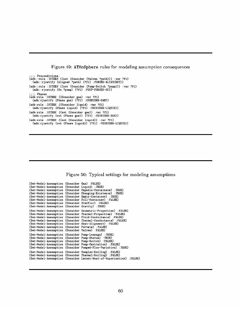
Figure 49: ATMoSphere rules for modeling assumption consequences

Preconditions:(adb : :rule :INTERN ((not (Consider (Valves ?path))) :var ?fl)

(adb : :rjustify (Aligned ?path) (?fl) :FORCED-ALIGNMENT))

(adb : :rule :INTERN ((not (Consider (Pump-Switch ?pump))) :var ?fl)(adb : :rjustify (On ?pump) (?fl) :PUMP-FORCED-ON))

Phases(adb :rule INTERN ((Consider gas) :var ?fl)

(adb :rjustify (Phase gas) (?fl) :CONSIDER-GAS))

(adb :rule INTERN ((Consider liquid) :var ?fl)(adb :rjustify (Phase liquid) (?fl) :CONSIDER-LIQUID))

(adb :rule INTERN ((not (Consider gas)) :var ?fl)(adb :rjustify (not (Phase gas)) (?fl) :CONSIDER-GAS))

(adb :rule INTERN ((not (Consider liquid)) :var ?fl)(adb :rjustify (not (Phase liquid)) (?fl) :CONSIDER-LIQUID))

Figure 50: Typical settings for modeling assumptions

(Set-Model-Assumption (Consider Gas) :FALSE)(Set-Model-Assumption (Consider Liquid) :TRUE)(Set-Model-Assumption (Consider Capable-Containers) :TRUE)(Set-Model-Assumption (Consider Changing-Existence) :TRUE)(Set-Model-Assumption (Consider Empty-Container) :TRUE)(Set-Model-Assumption (Consider Full-Container) :FALSE)(Set-Model-Assumption (Consider Overflow) :FALSE)(Set-Model-Assumption (Consider Gravity) :TRUE)

(Set-Model-Assumption (Consider Geometric-Properties) :FALSE)(Set-Model-Assumption (Consider Thermal-Properties) :FALSE)(Set-Model-Assumption (Consider Fluid-Conductance) :FALSE)(Set-Model-Assumption (Consider Thermal-Conductance) :FALSE)(Set-Model-Assumption (Consider Heat-Alignment) :FALSE)(Set-Model-Assumption (Consider Portals) :FALSE)(Set-Model-Assumption (Consider Valves) :FALSE)

(Set-Model-Assumption (Consider Pump-Lossage) :TRUE)(Set-Model-Assumption (Consider Pump-Status) :TRUE)(Set-Model-Assumption (Consider Pump-Switch) :FALSE)(Set-Model-Assumption (Consider Pump-Cavitation) FALSE)(Set-Model-Assumption (Consider Pumped-Flow-Variation) :TRUE)

(Set-Model-Assumption (Consider Complex-Boiling) FALSE)(Set-Model-Assumption (Consider Thermal-Boiling) FALSE)(Set-Model-Assumption (Consider Latent-Heat-of-Vaporization) :FALSE)

60

Figure 51: A path connecting two containers

Figure 52 : Scenario input for a path between two containers

(assertq (Substance WATER))

(assertq (Container CAN1))

(assertq (Container CAN2))

(assertq (Liquid-Path PATH1))

(assertq (Fluid-Connection PATH1 CAN1 CAN2))

The examples described below have been run under a variety of modeling assumptions.

For the sake of brevity, we list a "standard" set of assumptions in Figure 50 . For each

example, we indicate only the deviations from this standard set.

5 .1 Modeling a Simple Fluid Flow System

Here we describe a simple scenario consisting of two containers connected by a fluid path,

as depicted in Figure 51 . The corresponding scenario description is shown in Figure 52.

We define a substance: water ; two containers : CAN1 and CAN2 ; and a fluid-path: PATH1.

In addition, we specify that PATH1 connects CAN1 and CAN2.

We have envisioned this simple example under a variety of modeling assumptions . In

particular, we have toggled the consider assumptions for Thermal-Properties, Geometric-

Properties, Portals and Fluid-Conductance, both in isolation and in combination . The

results for these as well as the other examples discussed below are summarized in Table 1.

Run times for all examples were measured using a Symbolics 3670 running Genera 6 .2.

The presence of each modeling assumption enables a corresponding chunk of the model,

as detailed in Section 4 and summarized here . Considering Thermal-Properties causes

61

Figure 53 : Envisionment for simple flow with thermal properties

jti lt

I — —

I

I

'I

•

S3

I

I

•I

I I

AI S2 I

S5

1

S7

S8

•

•

•

•

•

•

•S4

S9

the contained liquids to posess the quantities heat and temperature, which are constrained

appropriately. Considering Geometric-Properties introduces comparisons between levels

of contained liquids and the top and bottom heights of their containers . Portals, when

considered, are created at the two ends of the path and used to reason about the flow

process . When the portals are at the bottoms of the containers, the resulting behavior is

the same as without portals . Considering Fluid-Conductance causes the conductance of

the path to be used in calculating flow rates.

The results in Table 1 demonstrate that as additional modeling assumptions are en-

abled, run times increase, as do the number of quantities, inequalities, and TMS structures

required to support the reasoning . Avoiding this extra complexity when it isn't needed is

of course the primary reason for introducing modeling assumptions into the domain model.

Figure 53 shows the envisionment produced when thermal properties are considered,

and Figure 54 shows the envisionment for the remaining cases . The other modeling as-

sumptions have no effect on the shape of the envisionment . Both envisionments are similar

in that flow into an empty container leads instantly to flow from higher to lower contained

liquid, which eventually leads to equilibrium. Considering thermal properties adds a dis-

0SO

Cold—to—Hot

62

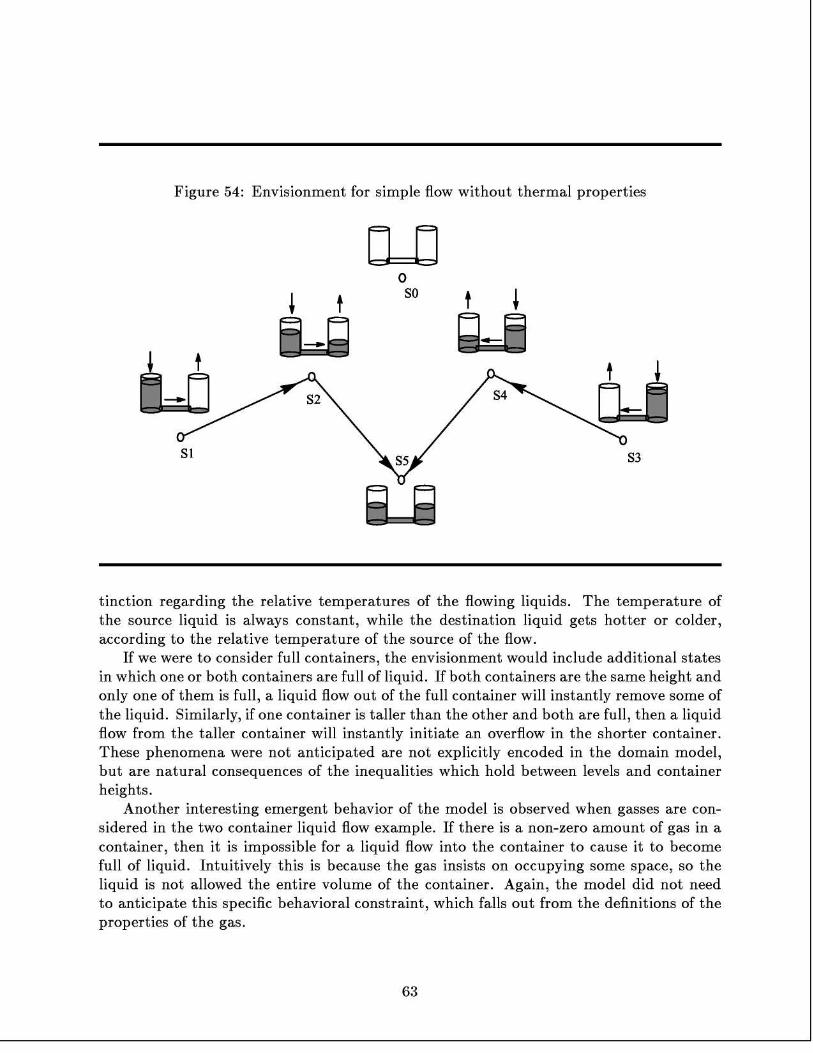
Figure 54 : Envisionment for simple flow without thermal properties

tinction regarding the relative temperatures of the flowing liquids . The temperature of

the source liquid is always constant, while the destination liquid gets hotter or colder,

according to the relative temperature of the source of the flow.

If we were to consider full containers, the envisionment would include additional states

in which one or both containers are full of liquid . If both containers are the same height and

only one of them is full, a liquid flow out of the full container will instantly remove some of

the liquid. Similarly, if one container is taller than the other and both are full, then a liquid

flow from the taller container will instantly initiate an overflow in the shorter container.

These phenomena were not anticipated are not explicitly encoded in the domain model,

but are natural consequences of the inequalities which hold between levels and container

heights.

Another interesting emergent behavior of the model is observed when gasses are con-

sidered in the two container liquid flow example . If there is a non-zero amount of gas in a

container, then it is impossible for a liquid flow into the container to cause it to become

full of liquid. Intuitively this is because the gas insists on occupying some space, so the

liquid is not allowed the entire volume of the container . Again, the model did not need

to anticipate this specific behavioral constraint, which falls out from the definitions of the

properties of the gas .

63

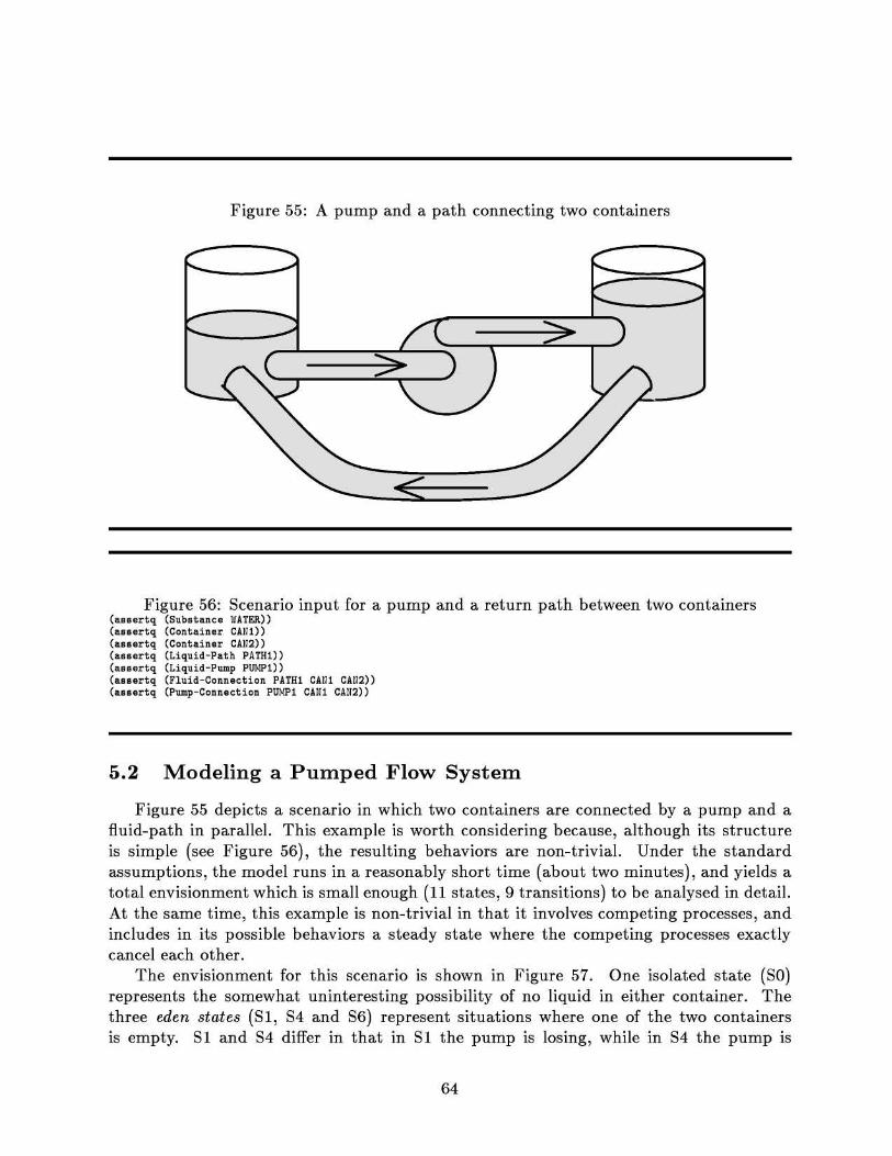
Figure 55 : A pump and a path connecting two containers

Figure 56 : Scenario input for a pump and a return path between two containers(assertq (Substance WATER))(assertq (Container CAN1))(assertq (Container CAN2))(assertq (Liquid-Path PATH1))(assertq (Liquid-Pump PUMP1))(assertq (Fluid-Connection PATH1 CAN1 CAN2))(assertq (Pump-Connection PUMP1 CAN1 CAN2))

5 .2 Modeling a Pumped Flow System

Figure 55 depicts a scenario in which two containers are connected by a pump and afluid-path in parallel . This example is worth considering because, although its structureis simple (see Figure 56), the resulting behaviors are non-trivial . Under the standardassumptions, the model runs in a reasonably short time (about two minutes), and yields atotal envisionment which is small enough (11 states, 9 transitions) to be analysed in detail.At the same time, this example is non-trivial in that it involves competing processes, andincludes in its possible behaviors a steady state where the competing processes exactlycancel each other.

The envisionment for this scenario is shown in Figure 57 . One isolated state (SO)represents the somewhat uninteresting possibility of no liquid in either container . Thethree eden states (S1, S4 and S6) represent situations where one of the two containersis empty. S1 and S4 differ in that in S1 the pump is losing, while in S4 the pump is

64

Figure 57 : Envisionment for the Pump Cycle example (without thermal properties)

65

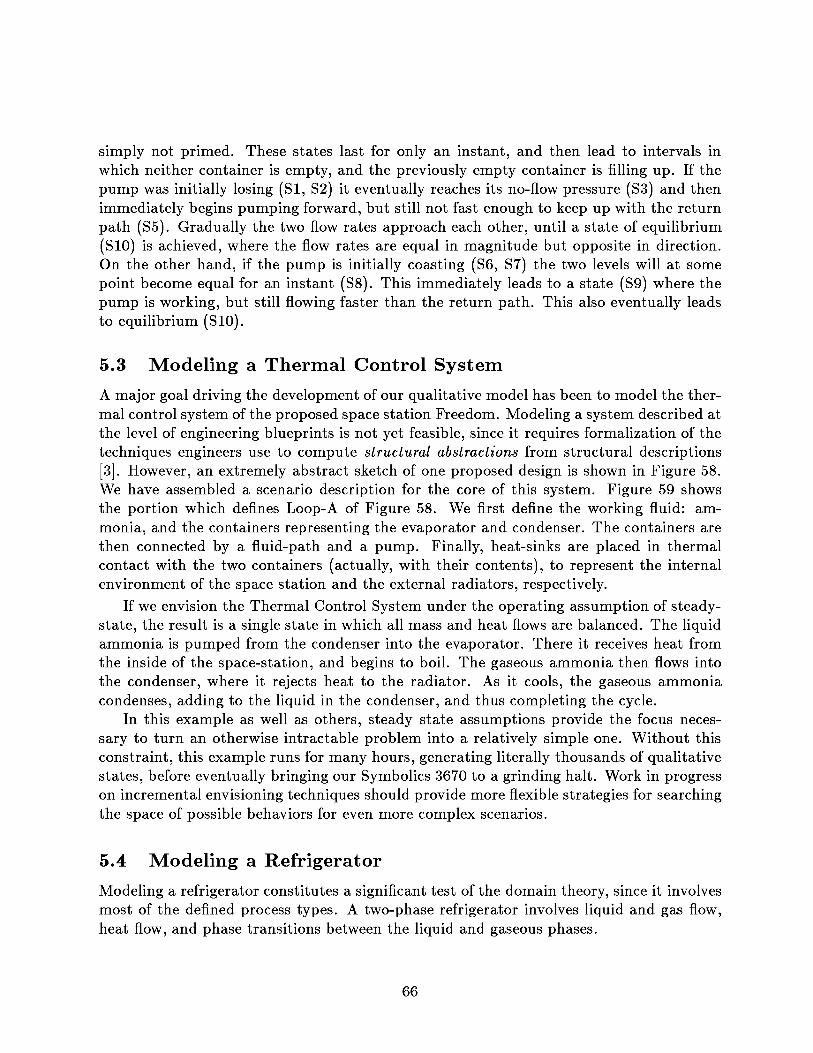
simply not primed . These states last for only an instant, and then lead to intervals inwhich neither container is empty, and the previously empty container is filling up . If thepump was initially losing (S1, S2) it eventually reaches its no-flow pressure (S3) and thenimmediately begins pumping forward, but still not fast enough to keep up with the returnpath (S5) . Gradually the two flow rates approach each other, until a state of equilibrium(S10 is achieved, where the flow rates are equal in magnitude but opposite in direction.On the other hand, if the pump is initially coasting (S6, S7) the two levels will at somepoint become equal for an instant (S8) . This immediately leads to a state (S9) where thepump is working, but still flowing faster than the return path . This also eventually leadsto equilibrium (S10).

5 .3 Modeling a Thermal Control System

A major goal driving the development of our qualitative model has been to model the ther-mal control system of the proposed space station Freedom. Modeling a system described atthe level of engineering blueprints is not yet feasible, since it requires formalization of thetechniques engineers use to compute structural abstractions from structural descriptions[3] . However, an extremely abstract sketch of one proposed design is shown in Figure 58.

We have assembled a scenario description for the core of this system . Figure 59 showsthe portion which defines Loop-A of Figure 58 . We first define the working fluid : am-monia, and the containers representing the evaporator and condenser . The containers arethen connected by a fluid-path and a pump. Finally, heat-sinks are placed in thermalcontact with the two containers (actually, with their contents), to represent the internalenvironment of the space station and the external radiators, respectively.

If we envision the Thermal Control System under the operating assumption of steady-state, the result is a single state in which all mass and heat flows are balanced . The liquidammonia is pumped from the condenser into the evaporator . There it receives heat fromthe inside of the space-station, and begins to boil . The gaseous ammonia then flows intothe condenser, where it rejects heat to the radiator . As it cools, the gaseous ammoniacondenses, adding to the liquid in the condenser, and thus completing the cycle.

In this example as well as others, steady state assumptions provide the focus neces-sary to turn an otherwise intractable problem into a relatively simple one . Without thisconstraint, this example runs for many hours, generating literally thousands of qualitativestates, before eventually bringing our Symbolics 3670 to a grinding halt . Work in progresson incremental envisioning techniques should provide more flexible strategies for searchingthe space of possible behaviors for even more complex scenarios.

5 .4 Modeling a Refrigerator

Modeling a refrigerator constitutes a significant test of the domain theory, since it involvesmost of the defined process types. A two-phase refrigerator involves liquid and gas flow,heat flow, and phase transitions between the liquid and gaseous phases.

66

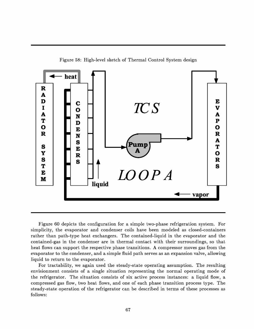
Figure 58: High-level sketch of Thermal Control System design

•- heat

TCS

PumpA .

LOOPAliquid

vapor

SYSTEM

C0NDE

SER

Figure 60 depicts the configuration for a simple two-phase refrigeration system. Forsimplicity, the evaporator and condenser coils have been modeled as closed-containersrather than path-type heat exchangers . The contained-liquid in the evaporator and thecontained-gas in the condenser are in thermal contact with their surroundings, so thatheat flows can support the respective phase transitions . A compressor moves gas from theevaporator to the condenser, and a simple fluid path serves as an expansion valve, allowingliquid to return to the evaporator.

For tractability, we again used the steady-state operating assumption . The resultingenvisionment consists of a single situation representing the normal operating mode ofthe refrigerator . The situation consists of six active process instances : a liquid flow, acompressed gas flow, two heat flows, and one of each phase transition process type . Thesteady-state operation of the refrigerator can be described in terms of these processes asfollows:

67

Figure 59: Scenario Description for TCS LOOP A:

;; Define working fluid:(assertq (substance NH3))

;; Define containers:(assertq (container EVAPORATOR-A))(assertq (container CONDENSER-A))

;; Set up expansion valve:(assertq (Gas-Path VAPOR-PATH-A))(assertq (Connects-to VAPOR-PATH-A EVAPORATOR-A CONDENSER-A))

;; Set up Pump:(assertq (Liquid-Pump PUMP-A))(assertq (Pump-Connection PUMP-A CONDENSER-A EVAPORATOR-A))

;; Set up heat-flow from Inside Space Station:(assertq (Heat-Sink INSIDE-STATION))(assertq (Heat-Path EVAP-SURFACE-A))(assertq (Thermally-Connects-To EVAP-SURFACE-A INSIDE-STATION (C-S NH3 liquid EVAPORATOR-A)))

;; Set up heat-flow to RADIATOR-SYSTEM(assertq (Heat-Sink RADIATOR-SYSTEM))(assertq (Heat-Path COND-SURFACE-A))(assertq (Thermally-Connects-To COND-SURFACE-A (C-S NH3 gas CONDENSER-A) RADIATOR-SYSTEM))

Figure 60: A two-phase refrigeration system

COMPRESSOR

•00 6) 000p ° ° °O0 0 0 0 0 0

°°°°ou °

o 0000

00000 00

INSIDE

FRIDGE

ooso ° ° oP° ° oo°°

0 0° °°o °

o 0 0 o 0 0o 00000

OUTSIDEWORLD

EVAPORATOREXPANSION

CONDENSER

VALVE

68

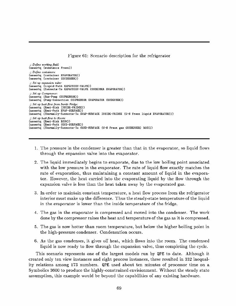
Figure 61 : Scenario description for the refrigerator

;; Define working fluid:(assertq (substance Freon))

;; Define containers:(assertq (container EVAPORATOR))(assertq (container CONDENSER))

;; Set up expansion valve:(assertq (Liquid-Path EXPANSION-VALVE))(assertq (Connects-To EXPANSION-VALVE CONDENSER EVAPORATOR))

;; Set up Compressor:(assertq (Gas-Pump COMPRESSOR))(assertq (Pump-Connection COMPRESSOR EVAPORATOR CONDENSER))

;; Set up heat-flow from Inside Fidge:(assertq (Heat-Sink INSIDE-FRIDGE))(assertq (Heat-Path EVAP-SURFACE))(assertq (Thermally-Connects-To EVAP-SURFACE INSIDE-FRIDGE (C-S Freon liquid EVAPORATOR)))

;; Set up heat-flow to Room:(assertq (Heat-Sink ROOM))(assertq (Heat-Path COND-SURFACE))(assertq (Thermally-Connects-To COND-SURFACE (C-S Freon gas CONDENSER) ROOM))

1. The pressure in the condenser is greater than that in the evaporator, so liquid flows

through the expansion valve into the evaporator.

2. The liquid immediately begins to evaporate, due to the low boiling point associated

with the low pressure in the evaporator . The rate of liquid flow exactly matches the

rate of evaporation, thus maintaining a constant amount of liquid in the evapora-

tor. However, the heat carried into the evaporating liquid by the flow through the

expansion valve is less than the heat taken away by the evaporated gas.

3. In order to maintain constant temperature, a heat flow process from the refrigerator

interior must make up the difference . Thus the steady-state temperature of the liquid

in the evaporator is lower than the inside temperature of the fridge.

4. The gas in the evaporator is compressed and moved into the condenser . The work

done by the compressor raises the heat and temperature of the gas as it is compressed.

5. The gas is now hotter than room temperature, but below the higher boiling point in

the high-pressure condenser . Condensation occurs.

6. As the gas condenses, it gives off heat, which flows into the room. The condensed

liquid is now ready to flow through the expansion valve, thus completing the cycle.

This scenario represents one of the largest models run by QPE to date . Although it

created only ten view instances and eight process instances, these resulted in 332 inequal-

ity relations among 173 numbers. QPE used about ten minutes of processor time on a

Symbolics 3600 to produce the highly-constrained envisionment . Without the steady state

assumption, this example would be beyond the capabilities of any existing hardware.

69

5 .5 Modeling a shipboard propulsion plant

Figure 62 depicts a greatly simplified model of a shipboard propulsion plant . We focuson the behavior of the fluid while in the boiler and immediately afterward. We ignorethe details surrounding the turbines, instead modeling them as a simple fluid path . Ourscenario description is given in Figure 63 . The boiler and superheater are both modeledas simple containers 20. The furnace is a heat-sink which is constrained to be hotter thanboth the liquid in the boiler and the gas in the superheater.

Because we are only interested in the behaviors in the boiler and superheater, we donot globally consider Thermal-Properties, but instead only consider it for those twocontainers . This prevents us from unnecessarily reasoning about thermal behaviors inthe feedwater tank or in the environment . If we were to consider Thermal-Propertiesglobally, we could still infer (with some effort) that the feedwater temperature is constant,but the thermal effect on the environment would be unconstrained.

Note that we cannot model the propulsion plant under the global assumption of steadystate, because it does not form a cycle . Thus in order for anything interesting to behappening, some quantities must be changing . But we can make use of some of the morespecific steady state assumptions . For example, we may reason about those states inwhich the quantities belonging to the fluid in the boiler or the superheater are constant,using the Stead-State-Individual consider assumption . Without these steady stateassumptions, there are eighteen possible combinations of active views and processes, andliterally thousands of completions in which all derivative values are known.

The constraints of partial steady state, along with the temperature relations shown inFigure 63, are sufficient to narrow the possibilities to three distinct situations, differingonly by the relative temperature of the steam flowing into the superheater . There are notransitions . In all three situations, water is being pumped from the feedwater tank intothe boiler, where it is converted into steam. The steam then flows into the superheater,where its temperature continues to rise, until it flows through the turbine and is dumpedinto the environment.

We believe that this model could provide the basis for answering questions such as:"Given an increase in feedwater temperature, what happens to the steam temperature atthe superheater outlet?" 21

5 .6 Summary of Examples

Table 1 summarizes the results of the examples described above . The table includes num-bers of states, transitions, quantities and inequalities, as well as run times and internalstatistics (numbers of nodes, environments and justifications) . These provide some indi-cation of the amount of inferencing going on "under the hood".

20Modeling heat exchangers correctly requires an alternate ontology for fluids—namely, our MolecularCollection Ontology, as discussed in [1].

'Understanding what happens in this situation is one of the hardest problems given at the U .S. NavySurface Warfare Officer's School, in NewPort, R .I .

70

B OILER

Figure 62 : A simplified shipboard propulsion plant

SUPER

HEATER

MMMMMMMMMMMMMMMMMMMMMMMMMMMMMMMMMMMMMMMMMMMMMMMMMMMMMMMMMMMMMMMMMMMM

FURNACEPUMP

Figure 63 : Scenario description for simplified propulsion plant

;; Define working fluid:(assertq (substance water))

;; Define Containers:(assertq (container FEEDWATER-TANK))(assertq (container BOILER))(assertq (container SUPERHEATER))(assertq (container ENVIRONMENT))

;; Setup Pump:(assertq (Liquid-Pump PUMP1))(assertq (Pump-Connection PUMP1 FEEDWATER-TANK BOILER))

;; Set up fluid paths to and from Superheater:(assertq (Gas-Path PATH1))(assertq (Connects-To PATH1 BOILER SUPERHEATER))(assertq (Gas-Path TURBINES))(assertq (Connects-To TURBINES SUPERHEATER ENVIRONMENT))

;; Set up heat-flows from FURNACE:(assertq (Heat-Sink FURNACE))(assertq (Heat-Path BOILER-SURFACE))(assertq (Thermally-Connects-To BOILER-SURFACE FURNACE (C-S Water liquid BOILER)))(assertq (Heat-Path SUPERHEATER-SURFACE))(assertq (Thermally-Connects-To SUPERHEATER-SURFACE FURNACE (C-S water gas SUPERHEATER)))

;; Make furnace HOT.(assertq

(less-than (A (temperature (C-S water liquid BOILER)

:absolute))

(assertq

(less-than(A(A

(temperature(temperature

furnace

:absolute))))(C-S water gas superheater)

:absolute))(A (temperature furnace

:absolute))))

71

Table 1:Example Sits Sclasses Trans Quants Ineqs Run-Time Nodes Justs Envs

2 Cans 6 6 4 21 57 78 (sec) 1087 1613 1912 Cans w/Portals 6 6 4 33 106 153 1743 3027 1792 Cans w/Thermal 12 10 16 35 89 154 1667 2566 3832 Cans w/Geometry 6 6 4 27 78 94 1381 2227 1922 Cans w/Conductance 6 6 4 27 69 152 1349 1997 5532 Cans w/Side-Portals 28 19 15 33 109 243 1833 3169 14462 Cans w/Portals,Conductanceand Thermal 12 10 16 49 142 266 2437 4077 908Pump-Cycle 11 11 9 23 66 117 1343 2091 572Pump-Cyclew/ Portals 11 11 9 41 151 332 2489 4946 1083TCS(steady state) 1 1 0 68 201 299 3687 5816 86Refrigerator 9 4 0 67 196 557 3663 6146 269Steam Plant 3 2 0 93 273 442 4697 7608 190

All of the examples presented here run in less than ten minutes, with the average runtime being just under four minutes . Without the ability to apply simplifying assumptions—primarily concerning steady state—several of the larger examples would be beyond thecapabilities of current hardware technology.

The examples presented here are intended to provide some indication of the capabilitiesof the FSThermo model, and by no means represent an exhaustive set . Given the com-posability offered by QP theory, the number of specific scenarios to which the FSThermomodel is applicable is limited only by the available computing resources.

6 Discussion

This paper has presented the FSThermo domain model for engineering thermodynamics.While certainly not the last word in qualitative models for engineering thermodynamics,we believe it represents substantial progress . Furthermore, we have tried to make themotivations for major design decisions explicit, and discussed the issues involved in devel-oping a large-scale qualitative domain model . While not a tutorial, we have tried to writedown some of the "lore" that has been accumulated by our group in developing domainmodels . We hope that other researchers might find this useful in developing their owndomain models .

72

While the FSThermo domain model captures a number of important phenomena inengineering thermodynamics, several extensions are needed to bring it closer to capturingthe full range of the qualitative aspect of an engineer's knowledge . These include:

Geometric knowledge: Currently no processes affect geometric properties . Thus theonly systems which can be described are those whose geometry is constant over time.Modeling many systems and components, such as internal combustion engines or flushtoilets, requires smoothly integrating a sophisticated dynamics with geometric reasoning.Kim [11,12] is working on such an integration.

Multiple substances : If we think only about the working fluid in a power plant, thesingle-substance assumption is not onerous . But more often multiple substances are re-quired. In some cases the interactions are thermal, and (assuming nothing is wrong) thesubstances do not mix . Examples include some lubrication systems and cooling systems.In other cases the chemical properties of the mixture are of paramount importance to themodel (e .g., distillation plants) . A general domain model for engineering thermodynamicsmust be able to model multiple substances.

As noted in Section 4 .2 .2, our current model has been designed with such extensionsin mind. In particular, the properties of the liquid-in and the gas-in for each con-tainer would be based on combinations of the properties of their constituents, rather thanequalities or constants . Chemical interactions between constituents need to be modeledby new processes, whose individuals are restricted to being contents of the same abstractindividual . We suspect that most of the non-chemical consequences of the properties ofthe liquid-in and the gas-in (e.g ., the interaction between the pressure of the gas-inand the pressure of the liquid-in) can remain unchanged.

Head: The current model presumes that the properties of the portals at the ends of apath suffice to establish whether or not there is a flow . If both portals are at the sameheight this presumption is correct, but otherwise it is not, since it does not take intoaccount the force of gravity acting on the fluid in the path itself. The current lack ofinternal geometric structure in fluid paths prevents us from modeling this.

In hydraulics the concept of head is introduced to properly account for the factors effect-ing flow through non-level paths . Within the perspective of contained-stuffs, head could bedefined qualitatively as the sum of pressure and height . This ignores any contribution fromvelocity, since the liquid in the path still is not explicitly represented . (Representing thevelocity of the liquid in the path would be easy with the molecular collection ontology, butproblematic within the contained-stuff view.) The minimal geometric extension to fluidpaths to support this definition of head would be to divide the path up into segments, andassociate a height with each segment.

New ontologies : Do the contained-stuff and molecular collection ontologies span thespace of entities needed for physical stuffs in engineering thermodynamics? Clearly not,

73

as our discussion of head indicates . Finding new ways to individuate pieces of stuff, todescribe fluid objects that are larger than molecular collections and not co-extensive withsome externally-defined container is an interesting open problem.

7 AcknowledgementsThis domain model incorporates many ideas developed in joint discussions with DennisDeCoste, Brian Falkenhainer, and Gordon Skorstad . This research was supported in partby the National Aeronautics and Space Administration, Contract No . NASA NAG-9137,by the Office of Naval Research, Contract No . N00014-85-K-0225, and by an NSF Presi-dential Young Investigator Award.

References[1] Collins, J. and Forbus, K . "Reasoning about Fluids via Molecular Collections", in

Proceedings of the National Conference on Artificial Intelligence, Seattle, July, 1987.

[2] de Kleer, J . and Brown, J . "A Qualitative Physics based on Confluences", ArtificialIntelligence, 24, 1984.

[3] Falkenhainer, B and Forbus, K . D . Setting up large-scale qualitative models . InProceedings of the Seventh National Conference on Artificial Intelligence, pages 301-306, St . Paul, MN, August 1988 . Morgan Kaufmann.

[4] Falkenhainer, B . and Forbus, K . "Compositional Modeling : Forming the relevantmodel for the job", submitted for publication, 1990.

[5] Forbus, K . "Qualitative Process Theory" Artificial Intelligence, 24, 1984.

[6] Forbus, K . "The Problem of Existence", in Proceedings of the Cognitive ScienceSociety, 1985.

[7] Forbus, K . "Introducing actions into qualitative simulation " , Proceedings of IJCAI-89,August, 1989.

[8] Forbus, K . D . The Qualitative Process Engine in Readings in Qualitative Reasoningabout Physical Systems, Weld, D . and de Kleer, J . (Eds .), Morgan Kaufmann, 1990.

[9] Hayes, P . "The Naive Physics Manifesto" , in Expert Systems in the Micro-ElectronicAge, D . Michie (Ed.), Edinburgh University Press, 1979.

[10] Hayes, P . "Naive Physics 1 : Ontology for Liquids " , in Hobbs, J . and Moore, B . (Eds .),Formal Theories of the Commonsense World, Ablex Publishing Corporation, 1985.

74

[11] Kim, H . "Qualitative Kinematics of Linkages " , Department of Computer ScienceTechnical Report No . UIUCDCS-R-90-1603.

[12] Kim, H. "Qualitative Reasoning about the Geometry of Fluid Flow", To appear inthe Proceedings of CogSci-90, July, 1990

[13] Kuipers, B . "Common Sense Causality : Deriving Behavior from Structure " , ArtificialIntelligence, 24, 1984.

[14] Kuipers, B . "Abstraction by Time-Scale in Qualitative Simulation " , in Proceedings ofthe National Conference on Artificial Intelligence, Seattle, July, 1987.

[15] Weld, D . " Switching Between Discrete and Continuous Process Models to PredictGenetic Activity" , MIT Artificial Intelligence Lab TR-793, October, 1984.

[16] Williams, B . "Qualitative Analysis of MOS Circuits", Artificial Intelligence, 24, 1984.

[17] Iwasaki, Y., and Simon, H . "Causality in Device Behavior" , Artificial Intelligence, 29,1986.

[18] Considine, D . M. (Ed.) Van Nostrand 's Scientific Encyclopedia, sixth edition, VanNostrand Reinhold Company, 1983 .

75