Building Proteins in a Day: Efficient 3D Molecular Reconstruction

Marcus A. Brubaker Ali PunjaniUniversity of Toronto

{mbrubake,alipunjani,fleet}@cs.toronto.edu

David J. Fleet

Abstract

Discovering the 3D atomic structure of molecules suchas proteins and viruses is a fundamental research problemin biology and medicine. Electron Cryomicroscopy (Cryo-EM) is a promising vision-based technique for structure es-timation which attempts to reconstruct 3D structures from2D images. This paper addresses the challenging prob-lem of 3D reconstruction from 2D Cryo-EM images. Anew framework for estimation is introduced which relieson modern stochastic optimization techniques to scale tolarge datasets. We also introduce a novel technique whichreduces the cost of evaluating the objective function dur-ing optimization by over five orders or magnitude. The netresult is an approach capable of estimating 3D molecularstructure from large scale datasets in about a day on a sin-gle workstation.

1. IntroductionDiscovering the 3D atomic structure of molecules such

as proteins and viruses is a fundamental research problemin biology and medicine. The ability to routinely determinethe 3D structure of such molecules would potentially revo-lutionize the process of drug development and accelerate re-search into fundamental biological processes. Electron Cry-omicroscopy (Cryo-EM) is an emerging vision-based ap-proach to 3D macromolecular structure determination thatis applicable to medium to large-sized molecules in their na-tive state. This is in contrast to X-ray crystallography whichrequires a crystal of the target molecule, which are often im-possible to grow [32] or nuclear magnetic resonance (NMR)spectroscopy which is limited to relatively small molecules[15].

The Cryo-EM reconstruction task is to estimate the 3Ddensity of a target molecule from a large set of images of themolecule (called particle images). The problem is similar inspirit to multi-view scene carving [6, 16] and to large-scale,uncalibrated multi-view reconstruction [1]. Like multi-viewscene carving, the goal is to estimate a dense 3D occupancyrepresentation of shape from a set of different views, but

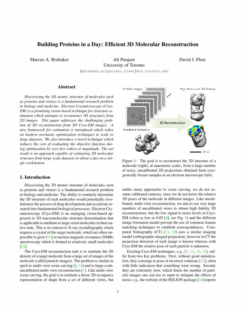
Figure 1: The goal is to reconstruct the 3D structure of amolecule (right), at nanometer scales, from a large numberof noisy, uncalibrated 2D projections obtained from cryo-genically frozen samples in an electron microscope (left).

unlike many approaches to scene carving, we do not as-sume calibrated cameras, since we do not know the relative3D poses of the molecule in different images. Like uncali-brated, multi-view reconstruction, we aim to use very largenumbers of uncalibrated views to obtain high fidelity 3Dreconstructions, but the low signal-to-noise levels in Cryo-EM (often as low as 0.05 [4]; see Fig. 1) and the differentimage formation model prevent the use of common featurematching techniques to establish correspondences. Com-puted Tomography (CT) [13, 10] uses a similar imagingmodel (orthographic integral projection), however in CT theprojection direction of each image is known whereas withCryo-EM the relative pose of each particle is unknown.

Existing Cryo-EM techniques, e.g., [7, 11, 34, 37], suf-fer from two key problems. First, without good initializa-tion, they converge to poor or incorrect solutions [12], oftenwith little indication that something went wrong. Second,they are extremely slow, which limits the number of parti-cles images one can use as input to mitigate the effects ofnoise; e.g., the website of the RELION package [34] reports

1

requiring two weeks on 300 cores to process a dataset with200,000 images.

We introduce a framework for Cryo-EM density estima-tion, formulating the problem as one of stochastic optimiza-tion to perform maximum-a-posteriori (MAP) estimation ina probabilistic model. The approach is remarkably efficient,providing useful low resolution density estimates in an hour.We also show that our stochastic optimization technique isinsensitive to initialization, allowing the use of random ini-tializations. We further introduce a novel importance sam-pling scheme that dramatically reduces the computationalcosts associated with high resolution reconstruction. Thisleads to speedups of 100,000-fold or more, allowing struc-tures to be determined in a day on a modern workstation. Inaddition, the proposed framework is flexible, allowing partsof the model to be changed and improved without impactingthe estimation; e.g., we compare the use of three differentpriors. To demonstrate our method, we perform reconstruc-tions on two real datasets and one synthetic dataset.

2. Background and Related WorkIn Cryo-EM, a purified solution of the target molecule

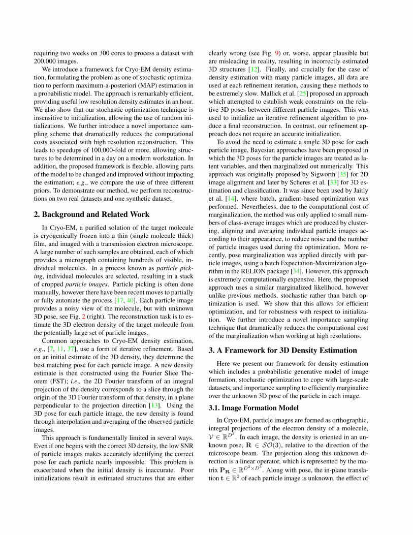
is cryogenically frozen into a thin (single molecule thick)film, and imaged with a transmission electron microscope.A large number of such samples are obtained, each of whichprovides a micrograph containing hundreds of visible, in-dividual molecules. In a process known as particle pick-ing, individual molecules are selected, resulting in a stackof cropped particle images. Particle picking is often donemanually, however there have been recent moves to partiallyor fully automate the process [17, 40]. Each particle imageprovides a noisy view of the molecule, but with unknown3D pose, see Fig. 2 (right). The reconstruction task is to es-timate the 3D electron density of the target molecule fromthe potentially large set of particle images.

Common approaches to Cryo-EM density estimation,e.g., [7, 11, 37], use a form of iterative refinement. Basedon an initial estimate of the 3D density, they determine thebest matching pose for each particle image. A new densityestimate is then constructed using the Fourier Slice The-orem (FST); i.e., the 2D Fourier transform of an integralprojection of the density corresponds to a slice through theorigin of the 3D Fourier transform of that density, in a planeperpendicular to the projection direction [13]. Using the3D pose for each particle image, the new density is foundthrough interpolation and averaging of the observed particleimages.

This approach is fundamentally limited in several ways.Even if one begins with the correct 3D density, the low SNRof particle images makes accurately identifying the correctpose for each particle nearly impossible. This problem isexacerbated when the initial density is inaccurate. Poorinitializations result in estimated structures that are either

clearly wrong (see Fig. 9) or, worse, appear plausible butare misleading in reality, resulting in incorrectly estimated3D structures [12]. Finally, and crucially for the case ofdensity estimation with many particle images, all data areused at each refinement iteration, causing these methods tobe extremely slow. Mallick et al. [25] proposed an approachwhich attempted to establish weak constraints on the rela-tive 3D poses between different particle images. This wasused to initialize an iterative refinement algorithm to pro-duce a final reconstruction. In contrast, our refinement ap-proach does not require an accurate initialization.

To avoid the need to estimate a single 3D pose for eachparticle image, Bayesian approaches have been proposed inwhich the 3D poses for the particle images are treated as la-tent variables, and then marginalized out numerically. Thisapproach was originally proposed by Sigworth [35] for 2Dimage alignment and later by Scheres et al. [33] for 3D es-timation and classification. It was since been used by Jaitlyet al. [14], where batch, gradient-based optimization wasperformed. Nevertheless, due to the computational cost ofmarginalization, the method was only applied to small num-bers of class-average images which are produced by cluster-ing, aligning and averaging individual particle images ac-cording to their appearance, to reduce noise and the numberof particle images used during the optimization. More re-cently, pose marginalization was applied directly with par-ticle images, using a batch Expectation-Maximization algo-rithm in the RELION package [34]. However, this approachis extremely computationally expensive. Here, the proposedapproach uses a similar marginalized likelihood, howeverunlike previous methods, stochastic rather than batch op-timization is used. We show that this allows for efficientoptimization, and for robustness with respect to initializa-tion. We further introduce a novel importance samplingtechnique that dramatically reduces the computational costof the marginalization when working at high resolutions.

3. A Framework for 3D Density EstimationHere we present our framework for density estimation

which includes a probabilistic generative model of imageformation, stochastic optimization to cope with large-scaledatasets, and importance sampling to efficiently marginalizeover the unknown 3D pose of the particle in each image.

3.1. Image Formation Model

In Cryo-EM, particle images are formed as orthographic,integral projections of the electron density of a molecule,V ∈ RD3

. In each image, the density is oriented in an un-known pose, R ∈ SO(3), relative to the direction of themicroscope beam. The projection along this unknown di-rection is a linear operator, which is represented by the ma-trix PR ∈ RD2×D3

. Along with pose, the in-plane transla-tion t ∈ R2 of each particle image is unknown, the effect of

Figure 2: A generative image formation model in Cryo-EM. The electron beam results in an orthographic integral projectionof the electron density of the specimen. This projection is modulated by the Contrast Transfer Function (CTF) and corruptedwith noise. The images pictured here showcase the low SNR typical in Cryo-EM. The zeros in the CTF (which completelydestroy some spatial information) make estimation particularly challenging, however their locations vary as a function ofmicroscope parameters. These are set differently across particle images in order to mitigate this problem. Particle imagesand density from [18].

which is similarly represented by a matrix St ∈ RD2×D2

.The resulting shifted projection is corrupted by two phe-nomena: a contrast transfer function (CTF) and noise. TheCTF is analogous to the effects of defocus in a conventionallight camera and can be modelled as a convolution of theprojected image. This linear operation is represented hereby the matrix Cθ ∈ RD2×D2

where θ are the parameters ofthe CTF model [30]. The Fourier spectrum of a typical CTFis shown in Figure 2; note the phase changes which resultin zero crossings (not typically observed in traditional lightcameras) and the attenuation at higher frequencies whichmakes estimation particularly challenging. CTF parame-ters, θ, are assumed to be given; CTF estimation is beyondthe scope of this work, but is routinely done using existingtools, e.g., [24, 27].

As noted above, and clearly seen in Figure 2, there isa large amount of noise present in typical particle images.This is primarily due to the sensitive nature of biologicalspecimens, requiring extremely low exposures. The noiseis modelled using an IID Gaussian distribution, resulting inthe following expression for the conditional distribution ofa particle image, I ∈ RD2

,

p(I | θ,R, t,V) = N (I |CθStPRV, σ2I) (1)

where σ is the standard deviation of the noise andN (·|µ,Σ)is the multivariate normal distribution with mean vector µand covariance matrix Σ.

In practice, due to computational considerations, Equa-tion (1) is evaluated in Fourier space, making use of the

Fourier Slice Theorem and Parseval’s Theorem to obtain

p(I | θ,R, t, V) = N (I | CθStPRV, σ2I) (2)

where I is the 2D Fourier transform of the image, St isthe shift operator in Fourier space (a phase change), Cθ

is the CTF modulation in Fourier space (a diagonal oper-ator), PR is a sinc interpolation operator which extracts aplane through the origin defined by the projection orienta-tion R and V is the 3D Fourier transform of V . To speed thecomputation of the likelihood, and due to the level of noiseand attenuation of high frequencies by the CTF, a maximumfrequency is specified, ω, beyond which frequencies are ig-nored.

The 3D pose, R, and shift, t, of each particle image areunknown and treated as latent variables which are marginal-ized out [35, 33]. Assuming R and t are independent ofeach other and the density V , one obtains

p(I | θ, V) =

∫R2

∫SO(3)

p(I|θ,R, t, V)p(R)p(t)dRdt

(3)where p(R) is a prior over 3D poses, R ∈ SO(3), and p(t)is a prior over translations, t ∈ R2. In general, nothing isknown about the projection direction so p(R) is assumed tobe a uniform distribution. Particles are picked to be closeto the center of each image, so p(t) is chosen to be a Gaus-sian distribution centered in the image. The above doubleintegral is not analytically tractable, so numerical quadra-ture is used [22, 9]. The conditional probability of an image

(likelihood) then becomes

p(I|θ, V) ≈MR∑j=1

wRj

Mt∑`=1

wtkp(I|θ,Rj , t`, V)p(R)p(t)

(4)where {(Rj , w

Rj )}MR

j=1 are weighted quadrature points overSO(3) and {(t`, wt

`)}Mt

`=1 are weighted quadrature pointsover R2. The accuracy of the quadrature scheme, and con-sequently the values of MR and Mt, are set automaticallybased on ω, the specified maximum frequency such thathigher values of ω results in more quadrature points.

Given a set of K images with CTF parameters D ={(Ii, θi)}Ki=1 and assuming conditional independence of theimages, the posterior probability of a density V is

p(V|D) ∝ p(V)

K∏i=1

p(Ii|θi, V) (5)

where p(V) is a prior over 3D molecular electron densities.Several choices of prior are explored below, but we foundthat a simple independent exponential prior worked well.Specifically, p(V) =

∏D3

i=1 λe−λVi where Vi is the value

of the ith voxel and λ is the inverse scale parameter. Otherchoices of prior are possible and is a promising direction forfuture research.

Estimating the density now corresponds to finding Vwhich maximizes Equation (5). Taking the negative logand dropping constant factors, the optimization problem be-comes arg minV∈RD3

+f(V),

f(V) = − log p(V)−K∑i=1

log p(Ii|θi, V) (6)

where V is restricted to be positive (negative density is phys-ically unrealistic). Optimizing Eq. (6) directly is costly dueto the marginalization in Eq. (4) as well as the large num-ber (K) of particle images in a typical dataset. To deal withthese challenges, the following sections propose the use oftwo techniques, namely, stochastic optimization and impor-tance sampling.

3.2. Stochastic Optimization

In order to efficiently cope with the large number ofparticle images in a typical dataset, we propose the useof stochastic optimization methods. Stochastic optimiza-tion methods exploit the large amount of redundancy inmost datasets by only considering subsets of data (i.e., im-ages) at each iteration by rewriting the objective as f(V) =∑k fk(V) where each fk(V) evaluates a subset of data.

This allows for fast progress to be made before a batch op-timization algorithm would be able to take a single step.

There are a wide range of such methods, ranging fromsimple stochastic gradient descent with momentum [28, 29,

36] to more complex methods such as Natural Gradientmethods [2, 3, 19, 20] and Hessian-free optimization [26].Here we propose the use of Stochastic Average GradientDescent (SAGD) [21] which has several important advan-tages. First, it is effectively self-tuning, using a line-searchto determine and adapt the learning rate. This is particu-larly important, as many methods require significant man-ual tuning for new objective functions and, potentially, eachnew dataset. Further, it is specifically designed for the finitedataset case allowing for faster convergence.

At each iteration τ , SAGD [21] considers only a singlesubset of data, kτ , which defines part of the objective func-tion fkτ (V) and its gradient gkτ (V). The density V is thenupdated as

Vτ+1 = Vτ −ε

KL

K∑j=1

dVτj (7)

where ε is a base learning rate, L is a Lipschitz constant ofgk(V), and

dVτk =

{gk(Vτ ) k = kτ

dVτ−1k otherwise(8)

is the most recent gradient evaluation of datapoint j at it-eration τ . This step can be computed efficiently by stor-ing the gradient of each observation and updating a run-ning sum each time a new gradient is seen. The Lipschitzconstant L is not generally known but can be estimated us-ing a line-search technique. Theoretically, convergence oc-curs for values of ε ≤ 1

16 [21], however in practice largervalues at early iterations can be beneficial, thus we useε = max( 1

16 , 21−bτ/150c). To allow parallelization and re-

duce the memory requires of SAGD, the data is divided intominibatches of 200 particles images. Finally, to enforce thepositivity of density, negative values of V are truncated tozero after each iteration. More details of the stochastic op-timization can be found in the Supplemental Material.

3.3. Importance Sampling

While stochastic optimization allows us to scale to largedatasets, the cost of computing the required gradient foreach image remains high due to the marginalization overorientations and shifts. Intuitively, one could consider ran-domly selecting a subset of the terms in Eq. (4) and usingthis as an approximation. This idea is formalized by impor-tance sampling (IS) which allows for an efficient and accu-rate approximation of the discrete sums in Eq. (4).1 A fullreview of importance sampling is beyond the scope of thispaper but we refer readers to [38].

1One can also apply importance sampling directly to the continuousintegrals in Eq. (3) but it can be computationally advantageous to precom-pute a fixed set of projection and shift matrices, PR and St, which can bereused across particle images.

To apply importance sampling, consider the inner sumfrom Eq. (4), rewriting it as

φRj =

Mt∑`=1

wt`pj,` =

Mt∑`=1

qt`

(wt`pj,`qt`

)(9)

where pj,` = p(I|θ,Rj , t`, V)p(Rj)p(t`) and qt =(qt1, . . . , q

tMt

)T is the parameter vector of a multinomial im-portance distribution such that

∑Mt

`=1 qt` = 1 and qt` > 0.

The domain of qt corresponds to the set of quadraturepoints in Equation (4). Then, φRj can be thought of as the

expected value E`[wt`pj,`qt`

] where ` is a random variable dis-

tributed according to qt. If a set of Nt � Mt randomindexes It are drawn according to qt, then

φRj ≈1

Nt

∑`∈It

wt`pj,`qt`

. (10)

Thus, we can efficiently approximate φRj by drawing sam-ples according to the importance distribution qR and com-puting the average. Using this approximation in Eq. (4)gives

p(I|θ, V) ≈MR∑j=1

wRj

1

Nt

(∑`∈It

wt`pj,`qt`

)(11)

and importance sampling can be similarly used for the outersummation to give

p(I|θ, V) ≈∑j∈IR

wRj

NRqRj

(∑`∈It

wt`

Ntqt`pj,`

)(12)

where IR are samples drawn from the importance distribu-tion qR = (qR1 , . . . , q

RMR

)T used for approximating

φt` =

MR∑j=1

wRj pj,` ≈

1

NR

∑j∈IR

wRj pj,`

qRj. (13)

The accuracy of the approximation in Eq. (12) is controlledby the number of samples used, with the error going tozero as N increases. We use N = s0s(q) samples wheres(q) =

(∑` q

2`

)−1is the effective sample size [8] and s0 is

a scaling factor. This choice ensures that when the impor-tance distribution is diffuse, more samples are used.

While the estimates provided by IS are unbiased, theirerror can be arbitrarily bad if the importance distribution isnot well chosen. To choose a suitable importance distribu-tion, we make two observations. First, the values φt` and φRjare proportional to the marginal probability of single parti-cle image having been generated with shift t` or pose Rj ,making them natural choices on which to base the impor-tance distributions. Second, these values remain stable once

0 2 4 6 8 10 12 141

0

1

2

3

4

5

KL

Div

erg

ence

(nats

)

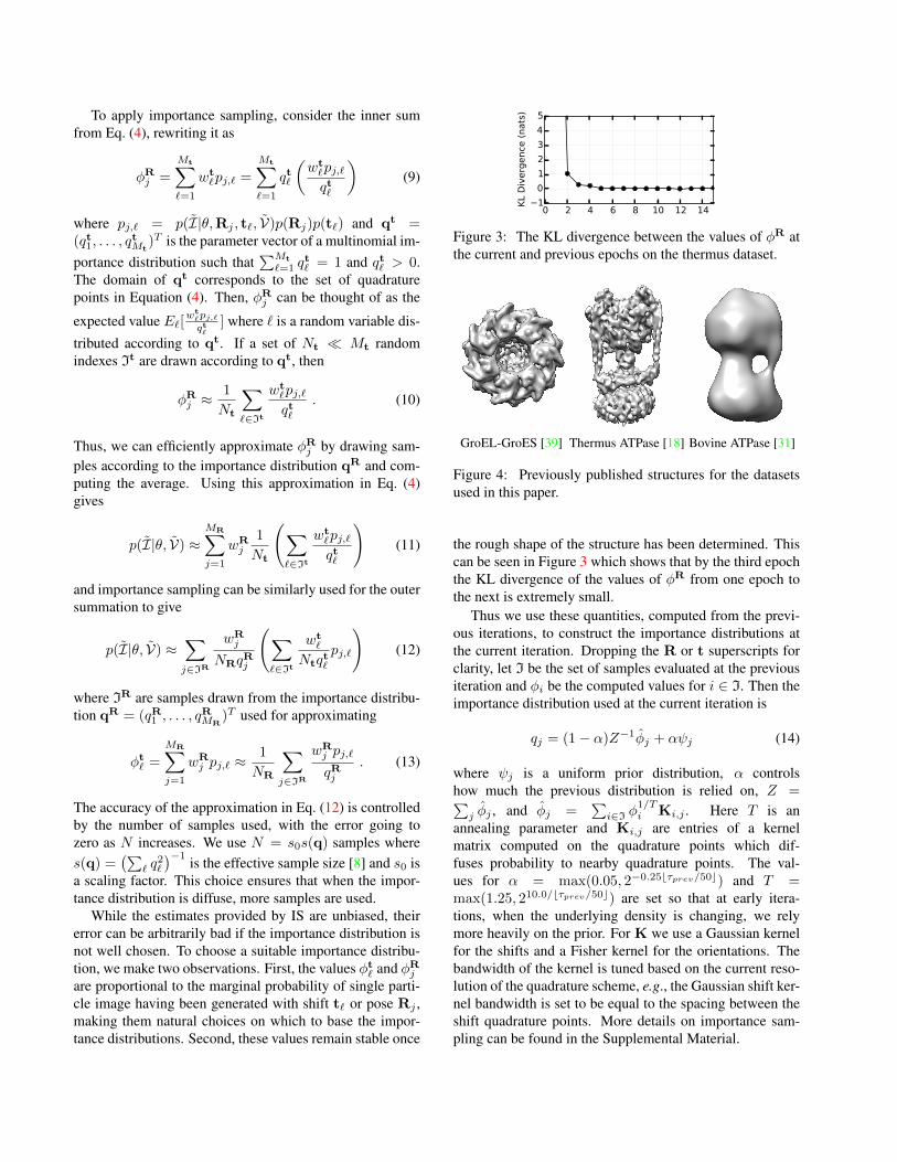
Figure 3: The KL divergence between the values of φR atthe current and previous epochs on the thermus dataset.

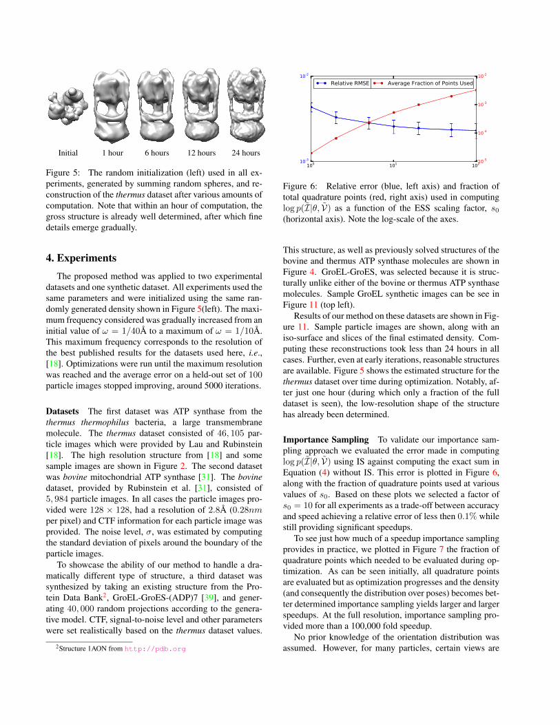
GroEL-GroES [39] Thermus ATPase [18] Bovine ATPase [31]

Figure 4: Previously published structures for the datasetsused in this paper.

the rough shape of the structure has been determined. Thiscan be seen in Figure 3 which shows that by the third epochthe KL divergence of the values of φR from one epoch tothe next is extremely small.

Thus we use these quantities, computed from the previ-ous iterations, to construct the importance distributions atthe current iteration. Dropping the R or t superscripts forclarity, let I be the set of samples evaluated at the previousiteration and φi be the computed values for i ∈ I. Then theimportance distribution used at the current iteration is

qj = (1− α)Z−1φj + αψj (14)

where ψj is a uniform prior distribution, α controlshow much the previous distribution is relied on, Z =∑j φj , and φj =

∑i∈I φ

1/Ti Ki,j . Here T is an

annealing parameter and Ki,j are entries of a kernelmatrix computed on the quadrature points which dif-fuses probability to nearby quadrature points. The val-ues for α = max(0.05, 2−0.25bτprev/50c) and T =max(1.25, 210.0/bτprev/50c) are set so that at early itera-tions, when the underlying density is changing, we relymore heavily on the prior. For K we use a Gaussian kernelfor the shifts and a Fisher kernel for the orientations. Thebandwidth of the kernel is tuned based on the current reso-lution of the quadrature scheme, e.g., the Gaussian shift ker-nel bandwidth is set to be equal to the spacing between theshift quadrature points. More details on importance sam-pling can be found in the Supplemental Material.

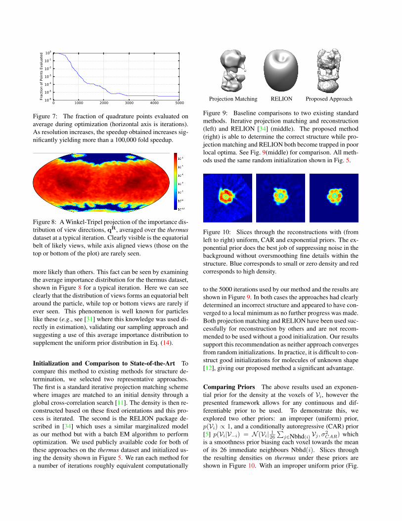
Initial 1 hour 6 hours 12 hours 24 hours

Figure 5: The random initialization (left) used in all ex-periments, generated by summing random spheres, and re-construction of the thermus dataset after various amounts ofcomputation. Note that within an hour of computation, thegross structure is already well determined, after which finedetails emerge gradually.

4. ExperimentsThe proposed method was applied to two experimental

datasets and one synthetic dataset. All experiments used thesame parameters and were initialized using the same ran-domly generated density shown in Figure 5(left). The maxi-mum frequency considered was gradually increased from aninitial value of ω = 1/40A to a maximum of ω = 1/10A.This maximum frequency corresponds to the resolution ofthe best published results for the datasets used here, i.e.,[18]. Optimizations were run until the maximum resolutionwas reached and the average error on a held-out set of 100particle images stopped improving, around 5000 iterations.

Datasets The first dataset was ATP synthase from thethermus thermophilus bacteria, a large transmembranemolecule. The thermus dataset consisted of 46, 105 par-ticle images which were provided by Lau and Rubinstein[18]. The high resolution structure from [18] and somesample images are shown in Figure 2. The second datasetwas bovine mitochondrial ATP synthase [31]. The bovinedataset, provided by Rubinstein et al. [31], consisted of5, 984 particle images. In all cases the particle images pro-vided were 128 × 128, had a resolution of 2.8A (0.28nmper pixel) and CTF information for each particle image wasprovided. The noise level, σ, was estimated by computingthe standard deviation of pixels around the boundary of theparticle images.

To showcase the ability of our method to handle a dra-matically different type of structure, a third dataset wassynthesized by taking an existing structure from the Pro-tein Data Bank2, GroEL-GroES-(ADP)7 [39], and gener-ating 40, 000 random projections according to the genera-tive model. CTF, signal-to-noise level and other parameterswere set realistically based on the thermus dataset values.

2Structure 1AON from http://pdb.org

100 101 10210-3

10-2

Relative RMSE

10-5

10-4

10-3

10-2

Average Fraction of Points Used

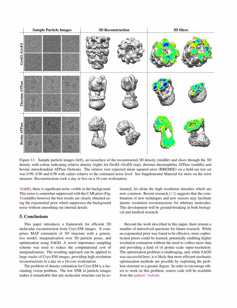
Figure 6: Relative error (blue, left axis) and fraction oftotal quadrature points (red, right axis) used in computinglog p(I|θ, V) as a function of the ESS scaling factor, s0(horizontal axis). Note the log-scale of the axes.

This structure, as well as previously solved structures of thebovine and thermus ATP synthase molecules are shown inFigure 4. GroEL-GroES, was selected because it is struc-turally unlike either of the bovine or thermus ATP synthasemolecules. Sample GroEL synthetic images can be see inFigure 11 (top left).

Results of our method on these datasets are shown in Fig-ure 11. Sample particle images are shown, along with aniso-surface and slices of the final estimated density. Com-puting these reconstructions took less than 24 hours in allcases. Further, even at early iterations, reasonable structuresare available. Figure 5 shows the estimated structure for thethermus dataset over time during optimization. Notably, af-ter just one hour (during which only a fraction of the fulldataset is seen), the low-resolution shape of the structurehas already been determined.

Importance Sampling To validate our importance sam-pling approach we evaluated the error made in computinglog p(I|θ, V) using IS against computing the exact sum inEquation (4) without IS. This error is plotted in Figure 6,along with the fraction of quadrature points used at variousvalues of s0. Based on these plots we selected a factor ofs0 = 10 for all experiments as a trade-off between accuracyand speed achieving a relative error of less then 0.1% whilestill providing significant speedups.

To see just how much of a speedup importance samplingprovides in practice, we plotted in Figure 7 the fraction ofquadrature points which needed to be evaluated during op-timization. As can be seen initially, all quadrature pointsare evaluated but as optimization progresses and the density(and consequently the distribution over poses) becomes bet-ter determined importance sampling yields larger and largerspeedups. At the full resolution, importance sampling pro-vided more than a 100,000 fold speedup.

No prior knowledge of the orientation distribution wasassumed. However, for many particles, certain views are

0 1000 2000 3000 4000 500010-6

10-5

10-4

10-3

10-2

10-1

100

Fract

ion o

f Poin

ts E

valu

ate

d

Figure 7: The fraction of quadrature points evaluated onaverage during optimization (horizontal axis is iterations).As resolution increases, the speedup obtained increases sig-nificantly yielding more than a 100,000 fold speedup.

Figure 8: A Winkel-Tripel projection of the importance dis-tribution of view directions, qR, averaged over the thermusdataset at a typical iteration. Clearly visible is the equatorialbelt of likely views, while axis aligned views (those on thetop or bottom of the plot) are rarely seen.

more likely than others. This fact can be seen by examiningthe average importance distribution for the thermus dataset,shown in Figure 8 for a typical iteration. Here we can seeclearly that the distribution of views forms an equatorial beltaround the particle, while top or bottom views are rarely ifever seen. This phenomenon is well known for particleslike these (e.g., see [31] where this knowledge was used di-rectly in estimation), validating our sampling approach andsuggesting a use of this average importance distribution tosupplement the uniform prior distribution in Eq. (14).

Initialization and Comparison to State-of-the-Art Tocompare this method to existing methods for structure de-termination, we selected two representative approaches.The first is a standard iterative projection matching schemewhere images are matched to an initial density through aglobal cross-correlation search [11]. The density is then re-constructed based on these fixed orientations and this pro-cess is iterated. The second is the RELION package de-scribed in [34] which uses a similar marginalized modelas our method but with a batch EM algorithm to performoptimization. We used publicly available code for both ofthese approaches on the thermus dataset and initialized us-ing the density shown in Figure 5. We ran each method fora number of iterations roughly equivalent computationally

Projection Matching RELION Proposed Approach

Figure 9: Baseline comparisons to two existing standardmethods. Iterative projection matching and reconstruction(left) and RELION [34] (middle). The proposed method(right) is able to determine the correct structure while pro-jection matching and RELION both become trapped in poorlocal optima. See Fig. 9(middle) for comparison. All meth-ods used the same random initialization shown in Fig. 5.

Figure 10: Slices through the reconstructions with (fromleft to right) uniform, CAR and exponential priors. The ex-ponential prior does the best job of suppressing noise in thebackground without oversmoothing fine details within thestructure. Blue corresponds to small or zero density and redcorresponds to high density.

to the 5000 iterations used by our method and the results areshown in Figure 9. In both cases the approaches had clearlydetermined an incorrect structure and appeared to have con-verged to a local minimum as no further progress was made.Both projection matching and RELION have been used suc-cessfully for reconstruction by others and are not recom-mended to be used without a good initialization. Our resultssupport this recommendation as neither approach convergesfrom random initializations. In practice, it is difficult to con-struct good initializations for molecules of unknown shape[12], giving our proposed method a significant advantage.

Comparing Priors The above results used an exponen-tial prior for the density at the voxels of Vi, however thepresented framework allows for any continuous and dif-ferentiable prior to be used. To demonstrate this, weexplored two other priors: an improper (uniform) prior,p(Vi) ∝ 1, and a conditionally autoregressive (CAR) prior[5] p(Vi|V−i) = N (Vi| 126

∑j∈Nbhd(i) Vj , σ

2CAR) which

is a smoothness prior biasing each voxel towards the meanof its 26 immediate neighbours Nbhd(i). Slices throughthe resulting densities on thermus under these priors areshown in Figure 10. With an improper uniform prior (Fig.

Sample Particle Images 3D Reconstruction 3D Slices

Gro

EL

-Gro

ES

The

rmus

ATPa

seB

ovin

eAT

Pase

Figure 11: Sample particle images (left), an isosurface of the reconstructed 3D density (middle) and slices through the 3Ddensity with colour indicating relative density (right) for GroEL-GroES (top), thermus thermophilus ATPase (middle) andbovine mitochondrial ATPase (bottom). The relative root expected mean squared error (RREMSE) on a held-out test setwas 0.99, 0.96 and 0.98 with values relative to the estimated noise level. See Supplemental Material for more on the errormeasure. Reconstructions took a day or less on a 16 core workstation.

10,left), there is significant noise visible in the background.This noise is somewhat suppressed with the CAR prior (Fig.10,middle) however the best results are clearly obtained us-ing the exponential prior which suppresses the backgroundnoise without smoothing out internal details.

5. ConclusionsThis paper introduces a framework for efficient 3D

molecular reconstruction from Cryo-EM images. It com-prises MAP estimation of 3D structure with a genera-tive model, marginalization over 3D particle poses, andoptimization using SAGD. A novel importance samplingscheme was used to reduce the computational cost ofmarginalization. The resulting approach can be applied tolarge stacks of Cryo-EM images, providing high resolutionreconstructions in a day on a 16-core workstation.

The problem of density estimation for Cryo-EM is a fas-cinating vision problem. The low SNR in particle imagesmakes it remarkable that any molecular structure can be es-

timated, let alone the high resolution densities which arenow common. Recent research [23] suggests that the com-bination of new techniques and new sensors may facilitateatomic resolution reconstructions for arbitrary molecules.This development will be ground-breaking in both biologi-cal and medical research.

Beyond the work described in this paper, there remain anumber of unresolved questions for future research. Whilean exponential prior was found to be effective, more sophis-ticated priors could be learned, potentially enabling higherresolution estimation without the need to collect more dataand providing a kind of of atomic-scale super-resolution.The optimization problem is challenging, and, while SAGDwas successful here, it is likely that more efficient stochasticoptimization methods are possible by exploiting the prob-lem structure to a greater degree. In order to encourage oth-ers to work on this problem, source code will be availablefrom the authors’ website.

Acknowledgements This work was supported in partby NSERC Canada and the CIFAR NCAP Program. MABwas funded in part by an NSERC Postdoctoral Fellowship.The authors would like thank John L. Rubinstein for pro-viding data and invaluable feedback.

References[1] S. Agarwal, N. Snavely, I. Simon, S. M. Seitz, and

R. Szeliski, “Building rome in a day,” in ICCV, 2009.

[2] S.-I. Amari, H. Park, and K. Fukumizu, “Adaptive methodof realizing natural gradient learning for multilayer percep-trons,” Neural Computation, vol. 12, no. 6, pp. 1399–1409,2000.

[3] S. Amari, “Natural gradient works efficiently in learning,”Neural Computation, vol. 10, no. 2, pp. 251–276, 1998.

[4] W. T. Baxter, R. A. Grassucci, H. Gao, and J. Frank, “Deter-mination of signal-to-noise ratios and spectral snrs in cryo-em low-dose imaging of molecules,” J Struct Biol, vol. 166,no. 2, pp. 126–32, May 2009.

[5] J. Besag, “Statistical analysis of non-lattice data,” Journalof the Royal Statistical Society. Series D (The Statistician),vol. 24, no. 3, pp. 179–195, 1975.

[6] R. Bhotika, D. Fleet, and K. Kutulakos, “A probabilistic the-ory of occupancy and emptiness,” in ECCV, 2002.

[7] J. de la Rosa-Trevın, J. Oton, R. Marabini, A. Zaldıvar,J. Vargas, J. Carazo, and C. Sorzano, “Xmipp 3.0: An im-proved software suite for image processing in electron mi-croscopy,” Journal of Structural Biology, vol. 184, no. 2, pp.321–328, 2013.

[8] A. Doucet, S. Godsill, and C. Andrieu, “On sequential MonteCarlo sampling methods for Bayesian filtering,” Statisticsand Computing, vol. 10, no. 3, pp. 197–208, 2000.

[9] M. Graf and D. Potts, “Sampling sets and quadrature formu-lae on the rotation group,” Numerical Functional Analysisand Optimization, vol. 30, no. 7-8, pp. 665–688, 2009.

[10] J. Gregson, M. Krimerman, M. B. Hullin, and W. Heidrich,“Stochastic tomography and its applications in 3d imagingof mixing fluids,” ACM Trans. Graph. (Proc. SIGGRAPH2012), vol. 31, no. 4, pp. 52:1–52:10, 2012.

[11] N. Grigorieff, “Frealign: high-resolution refinement of sin-gle particle structures,” J Struct Biol, vol. 157, no. 1, p.117–125, Jan 2007.

[12] R. Henderson, A. Sali, M. L. Baker, B. Carragher, B. De-vkota, K. H. Downing, E. H. Egelman, Z. Feng, J. Frank,N. Grigorieff, W. Jiang, S. J. Ludtke, O. Medalia, P. A.Penczek, P. B. Rosenthal, M. G. Rossmann, M. F. Schmid,G. F. Schroder, A. C. Steven, D. L. Stokes, J. D. Westbrook,W. Wriggers, H. Yang, J. Young, H. M. Berman, W. Chiu,G. J. Kleywegt, and C. L. Lawson, “Outcome of the first

electron microscopy validation task force meeting,” Struc-ture, vol. 20, no. 2, pp. 205 – 214, 2012.

[13] J. Hsieh, Computed Tomography: Principles, Design, Arti-facts, and Recent Advances. SPIE, 2003.

[14] N. Jaitly, M. A. Brubaker, J. Rubinstein, and R. H. Lilien, “ABayesian Method for 3-D Macromolecular Structure Infer-ence using Class Average Images from Single Particle Elec-tron Microscopy,” Bioinformatics, vol. 26, pp. 2406–2415,2010.

[15] J. Keeler, Understanding NMR Spectroscopy. Wiley, 2010.

[16] K. N. Kutulakos and S. M. Seitz, “A theory of shape by spacecarving,” IJCV, vol. 38, no. 3, pp. 199–218, 2000.

[17] R. Langlois, J. Pallesen, J. T. Ash, D. N. Ho, J. L. Rubin-stein, and J. Frank, “Automated particle picking for low-contrast macromolecules in cryo-electron microscopy,” Jour-nal of Structural Biology, vol. 186, no. 1, pp. 1 – 7, 2014.

[18] W. C. Y. Lau and J. L. Rubinstein, “Subnanometre-resolutionstructure of the intact Thermus thermophilus H+-driven ATPsynthase,” Nature, vol. 481, pp. 214–218, 2012.

[19] N. Le Roux and A. Fitzgibbon, “A fast natural Newtonmethod,” in ICML, 2010.

[20] N. Le Roux, P.-A. Manzagol, and Y. Bengio, “Topmoumouteonline natural gradient algorithm,” in NIPS, 2008, pp. 849–856.

[21] N. Le Roux, M. Schmidt, and F. Bach, “A stochastic gradi-ent method with an exponential convergence rate for stronglyconvex optimization with finite training sets,” in NIPS, 2012.

[22] V. J. Lebedev and D. N. Laikov, “A quadrature formula forthe sphere of the 131st algebraic order of accuracy,” DokladyMathematics, vol. 59, no. 3, pp. 477 – 481, 1999.

[23] X. Li, P. Mooney, S. Zheng, C. R. Booth, M. B. Braunfeld,S. Gubbens, D. A. Agard, and Y. Cheng, “Electron count-ing and beam-induced motion correction enable near-atomic-resolution single-particle cryo-em,” Nature Methods, vol. 10,no. 6, pp. 584–590, 2013.

[24] S. P. Mallick, B. Carragher, C. S. Potter, and D. J. Kriegman,“Ace: Automated {CTF} estimation,” Ultramicroscopy, vol.104, no. 1, pp. 8–29, 2005.

[25] S. P. Mallick, S. Agarwal, D. J. Kriegman, S. J. Belongie,B. Carragher, and C. S. Potter, “Structure and view estima-tion for tomographic reconstruction: A bayesian approach,”in CVPR, 2006.

[26] J. Martens, “Deep learning via hessian-free optimization,” inICML, 2010.

[27] J. A. Mindell and N. Grigorieff, “Accurate determinationof local defocus and specimen tilt in electron microscopy,”Journal of Structural Biology, vol. 142, no. 3, pp. 334–47,2003.

[28] Y. Nesterov, “A method of solving a convex programmingproblem with convergence rate o (1/k2),” Soviet MathematicsDoklady, vol. 27, no. 2, pp. 372–376, 1983.

[29] B. Polyak, “Some methods of speeding up the convergenceof iteration methods,” USSR Computational Mathematicsand Mathematical Physics, vol. 4, no. 5, pp. 1–17, 1964.

[30] L. Reimer and H. Kohl, Transmission Electron Microscopy:Physics of Image Formation. Springer, 2008.

[31] J. L. Rubinstein, J. E. Walker, and R. Henderson, “Struc-ture of the mitochondrial atp synthase by electron cryomi-croscopy,” The EMBO Journal, vol. 22, no. 23, pp. 6182–6192, 2003.

[32] B. Rupp, (2009). Biomolecular Crystallography: Principles,Practice and Application to Structural Biology. GarlandScience, 2009.

[33] S. H. W. Scheres, H. Gao, M. Valle, G. T. Herman, P. P. B.Eggermont, J. Frank, and J.-M. Carazo, “Disentangling con-formational states of macromolecules in 3d-em through like-lihood optimization,” Nature Methods, vol. 4, pp. 27–29,2007.

[34] S. H. Scheres, “RELION: Implementation of a Bayesianapproach to cryo-EM structure determination ,” Journal ofStructural Biology, vol. 180, no. 3, pp. 519 – 530, 2012.

[35] F. Sigworth, “A maximum-likelihood approach to single-particle image refinement,” Journal of Structural Biology,vol. 122, no. 3, pp. 328 – 339, 1998.

[36] I. Sutskever, J. Martens, G. Dahl, and G. Hinton, “On the im-portance of initialization and momentum in deep learning,”in ICML, 2013.

[37] G. Tang, L. Peng, P. Baldwin, D. Mann, W. Jiang, I. Rees,and S. Ludtke, “EMAN2: an extensible image processingsuite for electron microscopy,” Journal of Structural Biology,vol. 157, no. 1, pp. 38–46, 2007.

[38] S. T. Tokdar and R. E. Kass, “Importance sampling: areview,” Wiley Interdisciplinary Reviews: ComputationalStatistics, vol. 2, no. 1, pp. 54–60, 2010.

[39] Z. Xu, A. L. Horwich, and P. B. Sigler, “The crystal structureof the asymmetric GroEL-GroES-(ADP)7 chaperonin com-plex,” Nature, vol. 388, pp. 741–750, 1997.

[40] J. Zhao, M. A. Brubaker, and J. L. Rubinstein, “TMaCS:A hybrid template matching and classification system forpartially-automated particle selection,” Journal of StructuralBiology, vol. 181, no. 3, pp. 234 – 242, 2013.

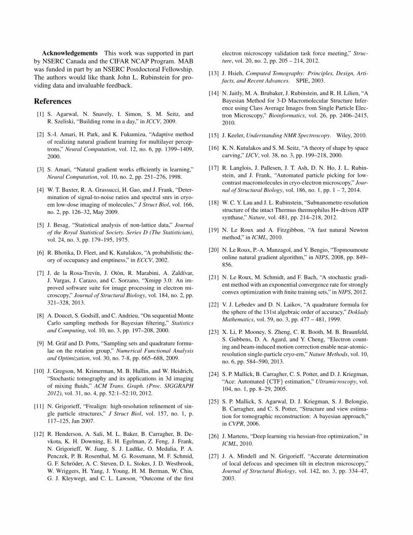
A. Stochastic OptimizationThis section provides algorithmic details of the Stochas-

tic Averaged Gradient Descent (SAGD) optimizationmethod used for MAP estimation. See the original SAGDpaper [21] for details. Consider the objective function spec-ified in Equation (6), rewritten as a sum of functions oversubsets of the data:

f(V) = − log p(V)−K∑i=1

log p(Ii|θi, V)

=

K∑i=1

[− 1

Klog p(V)− log p(Ii|θi, V)

]

=

K∑i=1

fi(V)

At each iteration τ , SAGD computes the update given by

Vτ+1 = Vτ −ε

L

K∑j=1

[dVτj −

1

K

∂

∂Vlog p(V)

]where dVτk is defined according to Equation (8). In practice,the sum in the above update equation is not computed ateach iteration, but rather a running total is maintained andupdated as follows:

gτ =

K∑k=1

dVτk

gτ+1 = gτ − dVτkτ + gkτ (Vτ )

The SAGD algorithm requires a Lipschitz constant Lwhich is not generally know. Instead it is estimated us-ing a line search algorithm where an initial value of L isincreased until the instantiated Lipschitz condition f(V) −f(V − L−1dV) < ‖dV‖2

2L is met. The line search for theLipschitz constant L is only performed once every 20 iter-ations. Note that a more sophisticated line search could beperformed if desired. A good initial value of L is found us-ing a bisection search where the upper bound is the smallestL found so far to satisfy the condition and the lower boundis the largest L found so far which fails the condition. Inbetween line searches, L is gradually decreased to try totake larger steps. The entire SAGD algorithm is provided inAlgorithm (1).

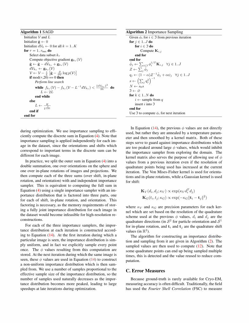
B. Importance SamplingImportance Sampling is a key part of the proposed recon-

struction method for Cryo-EM and provides large speedups

Algorithm 1 SAGDInitialize V and LInitialize g← 0Initialize dVk ← 0 for all k = 1..Kfor τ = 1..τmax do

Select data subset kτCompute objective gradient gkτ (V)g← g − dVkτ + gkτ (V)dVkτ ← gkτ (V)V ← V − ε

L

[g − ∂

∂V log p(V)]

if mod(τ ,20) == 0 thenPerform line search

while fkτ (V)− fkτ (V − L−1dVkτ ) <‖dVkτ ‖

2

2Ldo

L← 2Lend while

elseL← K

21

150

end ifend for

during optimization. We use importance sampling to effi-ciently compute the discrete sum in Equation (4). Note thatimportance sampling is applied independently for each im-age in the dataset, since the orientations and shifts whichcorrespond to important terms in the discrete sum can bedifferent for each image.

In practice, we split the outer sum in Equation (4) into adouble summation, one over orientations on the sphere andone over in-plane rotations of images and projections. Wethen compute each of the three sums (over shift, in-planerotation, and orientation) with and independent importancesampler. This is equivalent to computing the full sum inEquation (4) using a single importance sampler with an im-portance distribution that is factored into three parts, onefor each of shift, in-plane rotation, and orientation. Thisfactoring is necessary, as the memory requirements of stor-ing a fully joint importance distribution for each image inthe dataset would become infeasible for high-resolution re-constructions.

For each of the three importance samplers, the impor-tance distribution at each iteration is constructed accord-ing to Equation (14). At the first iteration during which aparticular image is seen, the importance distribution is sim-ply uniform, and in fact we explicitly sample every pointonce. The φ values resulting from this computation arestored. At the next iteration during which the same image isseen, these φ values are used in Equation (14) to constructa non-uniform importance distribution which is then sam-pled from. We use a number of samples proportional to theeffective sample size of the importance distribution, so thenumber of samples used naturally decreases as the impor-tance distribution becomes more peaked, leading to largespeedups at late iterations during optimization.

Algorithm 2 Importance SamplingGiven φi for i ∈ I from previous iterationfor j ∈ 1..J do

for i ∈ I doCompute Ki,j

end forend forφj ←

∑i∈I φ

1/Ti Ki,j ∀j ∈ 1..J

Z ←∑j φj

qj ← (1− α)Z−1φj + αψj ∀j ∈ 1..J

s←(∑

j q2j

)−1

N ← s0sI← ∅for k ∈ 1..N do

i← sample from qinsert i into I

end forUse I to compute φi for next iteration

In Equation (14), the previous φ values are not directlyused, but rather they are annealed by a temperature param-eter and then smoothed by a kernel matrix. Both of thesesteps serve to guard against importance distributions whichare too peaked around large φ values, which would inhibitthe importance sampler from exploring the domain. Thekernel matrix also serves the purpose of allowing use of φvalues from a previous iteration even if the resolution ofquadrature points being used has increased at the currentiteration. The Von Mises-Fisher kernel is used for orienta-tions and in-plane rotations, while a Gaussian kernel is usedfor shift:

KV (di, dj ;κV ) ∝ exp(κV dTi dj)

KG(ti, tj ;κG) ∝ exp(−κG‖ti − tj‖2)

where κV and κG are precision parameters for each ker-nel which are set based on the resolution of the quadraturescheme used at the previous φ values, di and dj are thequadrature directions (in S2 for particle orientation and S1for in-plane rotation, and ti and tj are the quadrature shiftvalues (in R2).

The algorithm for constructing an importance distribu-tion and sampling from it are given in Algorithm (2). Thesampled values are then used to compute (12). Note thatsome quadrature points can end up being sampled multipletimes, this is detected and the value reused to reduce com-putation.

C. Error MeasuresBecause ground-truth is rarely available for Cryo-EM,

measuring accuracy is often difficult. Traditionally, the fieldhas used the Fourier Shell Correlation (FSC) to measure

the resolution of a solved structure. The so-called gold-standard FSC works by splitting the dataset in half, estimat-ing two densities separately and the computing the normal-ized correlation in Fourier space as a function of frequency.This curve would then be thresholded to provide an estimateof accuracy. However, we note that this measure is actuallyestimating the variance of the estimator, not the accuracy ofthe density it has produced. Further it is only theoreticallyjustifiable when the estimator is unbiased, which is not trueof the method proposed here or with other likelihood-basedBayesian methods such as RELION.

Instead, we introduce a novel metric based on recon-struction error of a held test set. To quantify the ability ofmarginal likelihood methods, such as ours, to model andexplain the observed data we introduce the Expected MeanSquared Error

E2(I|θ,V) ≡ ER,t|I,θ,V[‖I −CθStPRV‖2

](15)

to be the expectation of the squared error between the im-age and its reconstruction under the image formation model.Note that the expectation is conditioned on the current den-sity and the CTF parameters and is taken over the unknownpose and translation, R and t. After switching to Fourierspace and with some manipulation E2(I|θ,V) becomes

Z−1∫R2

∫SO(3)

‖I−CθStPRV‖2p(I|θ,R, t, V)p(R)p(t)dRdt

(16)where the

Z =

∫R2

∫SO(3)

p(I|θ,R, t, V)p(R)p(t)dRdt (17)

is a normalization constant. Computing this would be com-putationally expensive, instead we use an importance sam-pling based approximation, E2(I|θ,V),

Z−1∑j∈IR

∑`∈It

wRj w

t`

NRqRj Ntqt`pj,`‖I − CθStPRV‖2 (18)

where

Z =∑j∈IR

∑`∈It

wRj w

t`

NRqRj Ntqt`pj,` (19)

is the approximation of the normalization constant. Theabove quantities can be readily computed along with themain likelihood computation using the same importancesampling scheme described above.

We compute the average value of E2(I|θ,V) on a heldout set of test images whose gradients are never used. Tonormalize for different datasets we report the Relative RootExpected Mean Squared Error (RREMSE) as√

1

σ2Ntest

∑IE2(I|θ,V) (20)

where the sum is taken over the test set which has Ntestimages and σ2 is the noise variance of the dataset. Valuesnear 1 indicate that the data is being well explained.