building homes, reviving neighborhoods: spillovers from ... · building homes, reviving...
TRANSCRIPT

Building Homes, Reviving Neighborhoods:Spillovers from Subsidized Construction of Owner-Occupied Housing in New York City
Ingrid Gould Ellen, Michael H. Schill, Scott Susin, and Amy Ellen Schwartz*
Abstract
This article examines the impact of two New York City homeownership programs on surrounding prop-erty values. Both programs, the Nehemiah Program and the Partnership New Homes program, subsi-dize the construction of affordable owner-occupied homes in distressed neighborhoods. We use a geocod-ed data set that includes every property transaction in the City from 1980 to 1999.
Our analysis relies on a difference-in-difference approach. Specifically, we compare the prices of proper-ties in small rings surrounding the Partnership and Nehemiah sites with prices of comparable proper-ties that are in the same ZIP code but outside the ring. We then examine whether the magnitude of thisdifference changes after the completion of a homeownership development. Our results show that duringthe past two decades prices of properties in the rings surrounding the homeownership projects haverisen relative to their ZIP codes. Results suggest that part of that rise is attributable to the affordablehomeownership programs.
Keywords: Homeownership; Housing prices; Neighborhood
Promoting homeownership has always been a central aim of housing policy in the UnitedStates. The federal tax code gives generous tax benefits to homeowners; the Federal HousingAdministration (FHA) provides insurance on high loan-to-value mortgages; a variety of otherFHA and state programs have offered below-market interest rates; and the Community Rein-vestment Act of 1977 provides incentives for financial institutions to make mortgage loansin low- and moderate-income communities. As cities have become more centrally involved inimplementing housing policy, local officials have begun to sponsor a large number of home-ownership programs in distressed communities.
Although, typically, these efforts do not reach the poorest households, they are justified in largepart by the positive spillovers that many argue will result from the development of new homes
Journal of Housing Research · Volume 12, Issue 2 185© Fannie Mae Foundation 2001. All Rights Reserved. 185
* Ingrid Gould Ellen is Assistant Professor of Public Policy and Urban Planning at New York University’s RobertF. Wagner Graduate School of Public Service. Michael H. Schill is Professor of Law and Urban Planning at the NewYork University School of Law and the Robert F. Wagner Graduate School of Public Service. Scott Susin is aResearch Fellow at the U.S. Bureau of the Census and a former Furman Fellow at the New York University Schoolof Law Center for Real Estate and Urban Policy. Amy Ellen Schwartz is Associate Professor of Public Policy at NewYork Univerity’s Robert F. Wagner Graduate School of Public Service.
The authors thank Denise DiPasquale, Frank DeGiovanni, and Eric Belsky for comments on an earlier draft andIoan Voicu for excellent research assistance. They also express their gratitude to Jerilyn Perine, Richard Roberts,Harold Shultz, and Calvin Parker of the New York City Department of Housing Preservation and Development andChuck Brass and Sal D’Avola of the New York City Housing Partnership for providing them with the data neces-sary to complete this research. The opinions and conclusions expressed here are those of the authors alone, and notof the U.S. Bureau of the Census or any other organization.
and by homeownership itself.1 There is little empirical evidence, however, about the effect thathome building and homeownership have on local communities. In this article we examine andcompare the effect that two of New York City’s major homeownership programs have had onproperty values in surrounding communities. Both of these programs, the Nehemiah Programand the New Homes program of the New York City Housing Partnership, subsidize the con-struction of affordable owner-occupied homes in distressed urban neighborhoods.
Several sections comprise this article; in the following section we discuss the channels throughwhich this type of subsidized construction could raise property values in the surroundingneighborhood, and we review the existing literature. In the methodology section we discussour hedonic-based “difference-in-difference” approach to identifying the effect of the home-ownership programs, controlling for structural features of the properties, neighborhoodamenities, and local housing market trends. In the summary of data section we describe therich data set analyzed here, which contains the sales prices and many structural character-istics of all properties sold in New York City during a period of almost 20 years. This study’smajor findings, the effect of the programs on neighborhood property values, are presented inthe results section. In the heterogeneity of effects section we break down these results, exam-ining the (potentially) varying effects of the two different programs, large versus small devel-opments, and developments built during boom or bust periods. In the conclusion we summa-rize the key results and discuss policy implications.
Spillover Effects of Homeownership and Housing Redevelopment
There are several reasons why the Nehemiah and the Partnership New Homes programsmight be expected to raise the value of surrounding properties. First, both replace blightedproperties or land with new structures. Unlike most commodities, housing is fixed in space,and the value of a home is therefore influenced not only by its structural features and qualitybut also by its surroundings. The appearance of neighboring homes, the level of noise and dis-order in a community, and the quality of local public services are all likely to contribute to thevalue of a particular home. Thus, housing investments in blighted areas should, in principle,generate spillover benefits that could be capitalized into the value of surrounding properties.
Second, these housing programs may have bolstered the number of homeowners in their com-munities, which may, in itself, lead to higher property values if, for example, homeowners’greater financial stake leads them to take better care of their homes than renters do.2 Sim-ilarly, homeowners may be more involved in local organizations and activities because of theirfinancial stake and/or because they tend to stay in their homes for a longer period of time.This involvement, again, may improve the quality of life in a community and raise propertyvalues.3
186 Ingrid Gould Ellen, Michael H. Schill, Scott Susin, and Amy Ellen Schwartz
1 Some cities may also support homeownership programs as an attempt to retain the middle class.
2 Absentee landlords have a financial stake in the property similar to homeowners.’ But the argument is that becauseabsentee landlords do not live in the property, they are not able to control the day-to-day upkeep in the same waythat homeowners can.
3 There is, in fact, little empirical evidence demonstrating that homeowners do make such social and economic in-vestments. (See Dietz and Haurin 2001; DiPasquale and Glaeser 1999; and Rohe, Van Zandt, and McCarthy 2000for evidence and discussion.)
These programs may also affect property values because of population change.Typically, home-owners earn higher incomes than renters and, thus, programs to increase homeownership in aneighborhood may also raise the community’s socioeconomic status. In addition, the programsmay increase property values as a result of the growth of population that occurs as vacantland is transformed into housing. This population growth may, in turn, lead to new com-mercial activity and economic growth, making the neighborhood more desirable.
Finally, as Galster (1987, 19) explains, exogenous changes to the “physical demographic char-acter of a neighborhood” may change expectations about the future of the community andinfluence individual mobility decisions and investments in upkeep.As vacant and derelict landis converted into habitable housing, nearby property owners may decide to remain in the com-munity rather than move away. They may also be more likely to invest in maintaining theirown homes, thereby generating additional positive neighborhood effects.4
There is little work that actually examines the neighborhood spillover effects generated by thesubsidized construction of owner-occupied homes. More work has focused on the relationshipbetween investments in publicly subsidized rental housing and neighborhood property val-ues. These studies offer conflicting evidence. Nourse (1963) and Rabiega, Lin, and Robinson(1984) have found that newly developed public housing can have modest positive effects onneighboring property values, whereas Lyons and Loveridge (1993); Goetz, Lam, and Heitlinger(1996); and Lee, Culhane, and Wachter (1999) all found small, statistically significant nega-tive effects on property values associated with the presence in a neighborhood of certain typesof federally subsidized housing. Moreover, in all these studies, data limitations make it dif-ficult to pinpoint the direction of causality. Are subsidized sites systematically located inweak (strong) neighborhoods, or does subsidized housing lead to neighborhood decline (im-provement)? Typically, these studies compare price levels in neighborhoods with subsidizedhousing to price levels in neighborhoods without subsidized housing, but it is difficult toknow whether the two groups of neighborhoods are truly comparable.
Two more recent studies of subsidized rental housing have made strides in overcoming thiscausality problem. Briggs, Darden, and Aidala (1999) examined the early effects that seven scat-tered-site public housing developments had on property values in neighborhoods in Yonkers,NY. Using a pre/post design with census tract fixed effects, they found little effect on the sur-rounding area. Santiago, Galster, and Tatian (2001) examined whether the acquisition andrehabilitation of property to create scattered-site public housing in Denver influenced thesales prices of surrounding single-family homes. These authors also used a pre/post designwith localized fixed effects and found that, typically, proximity to dispersed public housingunits is, if anything, associated with an increase in the prices of single-family homes.5
In short, there is no consensus about the effects that investments in subsidized rental housinghave on surrounding property values, although recent research suggests negligible or small
Spillovers from Subsidized Construction of Owner-Occupied Housing 187
4 All these changes are also likely to increase the flow of capital into the neighborhood by decreasing risk. Thisincrease in the availability of bank financing for home purchase and improvement loans is likely to increase theliquidity and price of housing in the neighborhood. It will also facilitate unsubsidized rehabilitation of housing (Gal-ster 1987).
5 Santiago, Galster, and Tatian (2001) also controlled for past trends in housing prices in the immediate vicinity ofa project; therefore, they tested for changes both in price levels and trends after completion. (This methodology wasshown first in Galster, Tatian, and Smith 1999.)

positive effects. As noted, research on the spillover effects of homeownership programs is farthinner. We found only two studies that examine the effect of publicly assisted homeowner-ship programs.6 Lee, Culhane, and Wachter (1999) found that FHA-insured units and units de-veloped through the Philadelphia Housing Authority’s homeownership program both havepositive effects on surrounding house prices.That finding is precisely the opposite of the study’soverall conclusions concerning rental housing (see above).7 Cummings, DiPasquale, and Kahn(2000) studied the effect of two Nehemiah housing developments in Philadelphia. Using meth-ods somewhat similar to ours, the authors compared price trends in the census tracts that con-tained these developments with trends in similarly distressed tracts elsewhere in the City.8
They found no statistically significant spillover effects, but because they had only two devel-opments in the City to evaluate, their confidence intervals are quite wide, and they can ruleout neither large positive nor large negative effects.9
New York City Housing Programs
In 1986, New York City launched an unprecedented initiative to rebuild the housing stock thathad been devastated in the 1970s. Between 1987 and mid-1999 the city’s housing agency, theDepartment of Housing Preservation and Development (HPD), invested close to $5 billion inthe construction of more than 22,000 homes, the gut rehabilitation of more than 43,000 unitsof formerly vacant housing, and the moderate rehabilitation of more than 97,000 units ofoccupied housing.10 Most of these efforts have focused on low- and moderate-income rentalhousing, but a few programs sponsor ownership housing.
Nehemiah Program
The Nehemiah Program was launched in the early 1980s by East Brooklyn Congregations,a group of 36 churches in Brooklyn. Typically, the Nehemiah Program built projects consist-ing of 500 to 1,000 units each on large tracts of donated city-owned land. Generally, the unitsare quite modest, built in identical block-long rows of single-family, 18-foot-wide homes. Thefirst house was completed in 1984; nearly 3,000 homes have been built in total. About 80 per-cent of these homes were built in Brooklyn; the rest of them, built by another group of church-es, are in the South Bronx (Stuart 1997).
188 Ingrid Gould Ellen, Michael H. Schill, Scott Susin, and Amy Ellen Schwartz
6 Many argue that an increase in the proportion of homeowners should in itself bolster property values. Is the valueof a property higher (or does it appreciate more rapidly) when it is located in a community with a greater share ofhomeowners? Few studies tackle that question, again perhaps because of concerns about endogeneity. In an analysisof 2,600 nonaffluent urban census tracts between 1980 and 1990, Rohe and Stewart (1996) found that housingprices appreciated more rapidly in neighborhoods with higher homeownership rates. They did not, however, analyzethe root causes of that effect.
7 The Section 8 New Construction Program is the only rental housing program that they found to be correlated withhigher property values.
8 The key difference between their approach and ours is that they did not control for previous trends in housing val-ues near the developments and relied on census tract geocoding rather than measuring the actual distance betweenthe sale and the homeownership development.
9 Their article also provides an interesting analysis of the benefits delivered to individual homeowners.
10 These figures are estimates of activity beginning in fiscal year 1987 and ending in fiscal year 1998.
The high-volume, mass-production approach has allowed the Nehemiah Program to deliverunits at a very low cost. Units cost from $60,000 to $70,000 to build, and the purchase pricewas lowered by $10,000 to $15,000 through a non-interest-bearing second mortgage from theCity, due only on resale (Donovan 1994; Orlebeke 1997). Estimates of the average incomes ofthe families who moved into the Nehemiah homes range from $27,000 to $31,000, which issomewhat higher than the 1990 average family income (under $25,000) of census tracts inwhich the homes were built.
Partnership New Homes Program
The New York City Housing Partnership is a not-for-profit intermediary organized in 1982 tohelp create and manage an affordable homeownership production program in the City (Wylde1999). Its core program—the New Homes program—was launched soon after to develop new,affordable owner-occupied homes in distressed communities. Partnership homes were builtby private, profit-motivated developers selected by the City and the Partnership. Most Part-nership projects consist of fewer than 100 units, and many are located on small infill sitesgrouped together to make up a project (Orlebeke 1997). The typical Partnership developmentcontains two- and three-family homes that include an owner’s unit plus one or two rentalunits.
According to one 1988 study of 10 Partnership projects, per-unit costs during the 1980s rangedfrom $57,000 to $137,000 (Orlebeke 1997). On average, the income of the residents movinginto Partnership homes in 1990 was $32,000, again somewhat higher than the mean incomeof their surrounding neighborhoods. In all Partnership projects the City provided the land ata nominal cost ($500 per lot) and gave a $10,000 subsidy per home; the State AffordableHousing Corporation provided an additional $15,000 per home (Donovan 1994).
By June 1999, the Partnership New Homes program had added 12,590 new homes, like theNehemiah Program, primarily in Brooklyn and the Bronx. But roughly one-quarter of thehomes have been built in New York City’s three other boroughs.
Choosing Locations
In testing the effect of new housing on surrounding areas there is always some concern aboutsite selection. Here, for example, the City may have tried to select “strong” sites for new hous-ing, areas in which it believed property values were beginning to increase (or had promise inthe near future). Even if the City had wanted to do so, however, there were considerable con-straints limiting the choice of locations. First, the site had to be city-owned, which means ithad been abandoned by its previous owner and vested in an in rem proceeding for delinquentproperty taxes. Because private owners were much less likely to have abandoned propertiesin more promising areas, the City’s stock of abandoned properties was overwhelmingly con-centrated in its poorest neighborhoods (Scafidi et al. 1998). Second, in the case of the Nehemi-ah Program, the land had to be a large, mostly vacant contiguous parcel.
Furthermore, as interviews with city officials suggest, the City did not give its best vacant sitesto the Partnership and Nehemiah sponsors. In many instances the City was interested inrealizing a high return from its land holdings and in minimizing the total subsidy required for
Spillovers from Subsidized Construction of Owner-Occupied Housing 189
redevelopment. As Anthony Gliedman, former HPD commissioner expressed it, “Why wouldwe do market-rate sites with the Partnership?” (Orlebeke 1997). In other words, the processof selecting individual sites, although perhaps not fully random, was certainly far from onethat sought to systematically pick winners. Rather, there is reason to believe that the Citychose losers, suggesting that our spillover estimates would provide conservative estimates ofthe effect of randomly sited housing. Nonetheless, our research design includes various con-trols for systematic selection issues.
Methodology
The centerpiece of this research is a hedonic price function that views housing as a compositegood or a bundle of services. Observed house prices are the product of the quantity of hous-ing services attached to the property and the price of these housing services, summed overall structural and location characteristics of the property. The basic model takes the follow-ing form:
Pit = α + βXit + γZit + δIt + εit, (1)
where P is the sales price of the property; X is a vector of property-related characteristics, in-cluding age and structural characteristics; Z is a vector of location attributes, such as localpublic services and neighborhood conditions; I is a vector of dummy variables indicating theyear of the sale; i indexes properties; and t indexes time. As usual α represents an interceptand β, γ, and δ represent vectors of parameters to be estimated; ε represents an error term.11
The derivative of the housing price function with respect to an individual attribute may thenbe interpreted as the implicit price of that attribute (Rosen 1974). In many cases housing pricesare entered as logarithms (as we do below), so that the coefficients are interpreted as thepercentage change in price resulting from an additional unit of the independent variable. Inthe case of a dummy variable, the coefficient can be interpreted as the difference in log pricebetween properties that have the attribute and those that do not. The difference in log priceclosely approximates the percentage difference in price when the difference is small enough.For the differences discussed in this article, which are generally smaller than 10 percent, theapproximation is close, so we use this more intuitive interpretation.12
As suggested above, the price of housing is affected by a broad array of structural and neigh-borhood characteristics, and, therefore, estimating equation 1 requires a great deal of detaileddata. Unfortunately, if some relevant variables cannot be included, either because they areunmeasured or because data are unavailable, the coefficients on the included variables may bebiased. Thus, our challenge in trying to identify the independent effect of proximity to Part-nership and Nehemiah homes is to control for a sufficient number of neighborhood attrib-utes so that our impact estimates do not suffer from omitted variable bias.
190 Ingrid Gould Ellen, Michael H. Schill, Scott Susin, and Amy Ellen Schwartz
11 In principle, spatial autocorrelation in the error term, although not biasing the regression coefficients, couldcause the standard errors we report to be underestimated (see e.g., Can and Megbolugbe 1997). However, we expectthat after controlling for ZIP code–quarter effects and also detailed building characteristics, little spatial autocor-relation will be left. Basu and Thibodeau (1998) estimated a hedonic regression and found only modest spatial auto-correlation, even using less-fine-grained geographic controls than ours.
12 The exact percentage effect of a difference in logs, b, is given by 100(eb – 1), although this formula is itself an approx-imation when b is a regression coefficient; see Halvorsen and Palmquist (1980) and Kennedy (1981).
Our basic approach is to adapt the Galster, Tatian, and Smith (1999) model, estimating thedifference between prices of properties in the microneighborhoods (or rings) surrounding Ne-hemiah and Partnership sites and the prices of comparable properties that are outside thering, but still located in the same general neighborhood. Then we examine whether the mag-nitude of this difference has changed over time and, if so, whether the change is associatedwith the completion of a Partnership or Nehemiah project.13 This approach should yield an un-biased measure of impact if (1) sufficient data on the structural characteristics of the homesthat sell are available and (2) other neighborhood influences that shaped the value of prop-erties very near the Partnership and Nehemiah sites at about the time of project completionsimilarly influenced property values in the general neighborhood.
More specifically, we supplement the model above with variables identifying properties in thering of the housing investments (variables that capture the price differential between prop-erties inside and outside the ring) and by specifying those variables to allow the price differ-ential to change over time. As always, there is no single best way to specify these variables.Instead, different specifications reflect different counterfactuals and offer distinct advantages.
As described in greater detail below, our response is to estimate several alternative specifi-cations of the model, reflecting a range of choices and alternatives. More specifically, we esti-mate the model for three different ring sizes—a 500-foot ring, 1,000-foot ring, and 2,000-footring—that define properties in the vicinity of Nehemiah or Partnership sites. We also inves-tigate three alternative ways of capturing differentials in price levels and trends between prop-erties inside and outside the ring. Our first specification includes a different ring dummy foreach of the 9 preceding years, with another dummy indicating 10 or more previous years.There is also a similar set of 10 dummies for the following years, and another for the year ofcompletion. This parameterization provides estimates of the price differential between theinside and outside of the ring in each of 21 years (multiyear periods in the case of the two outerdummies). Our second, more parsimonious, specification generates an overall before-aftercomparison by replacing these 21 ring-year dummy variables with a single “ever in the ring”dummy variable, an in-ring postcompletion dummy variable, and a postcompletion trendvariable. A third specification includes controls for previous trends in the price differentialinside and outside the rings before the development of the new homes (using a spline speci-fication to allow for different trends in different time periods). Thus, the third specificationprovides an estimate in which the counterfactual is that the price gap between the ring andthe neighborhood would have continued to shrink (or grow) at the precompletion rate if noproject had been completed.
As noted, we think each of these specifications offers distinct advantages and, therefore, weshow the results from all three. The first is the most flexible, offering a detailed view of pricechanges over time, but the large number of coefficients makes it difficult to summarize theoverall effect. The second is more parsimonious and straightforward, but it may be oversim-plistic and fail to account for trends in the ring-neighborhood price gap before the comple-tion of the project. The third specification controls for these previous trends and thereby helpsto mitigate concerns about selection bias, but it may be overconservative. Because propertyvalues may begin to rise once a project is announced or started, the trends may also pick upsome of the effects of the developments themselves, in anticipation of the effect the project
Spillovers from Subsidized Construction of Owner-Occupied Housing 191
13 Thus, we form a difference-in-difference impact estimate. The impact of the housing investment is identified asthe difference between properties inside and outside the ring, before and after the housing investment.
will have on the surrounding community.14 (According to HPD staff, community residentswere involved in the planning process and often they knew about these projects years beforethe start of construction.) If so, including the splines means that we measure just the addedeffect a project’s completion has on property values, above and beyond the effect of its com-pletion or start, and that we understate its full effect.
Unfortunately, it is impossible to know whether, in fact, previous trends in prices in the ringrelative to those in the ZIP code would have continued at the same rate if the project had notbeen constructed. In our third specification, we effectively assume that the trend in relativeprices that occurred during the five years before project completion would have continued inthe years after completion. In our second specification, we assume that prices in the ringswould have increased at the same rate as prices in the ZIP code. It is likely that neither ofthose assumptions is fully accurate, but it is impossible to know what would have happenedto prices in the rings in the absence of the newly built homes.15
Mathematically, our first model can be written as follows:
LnP = α + βX + δZIPcode–Quarter + γRing_Years_From_Sale + ε, (2)
where X is a vector of structural characteristics, as before, and ZIPcode–Quarter is a vectorof dummy variables indicating the neighborhood in which the property is located (measuredby ZIP code) and the year and quarter of sale (for example, first quarter 1980, second quarter1980, and so on).16 These ZIPcode–Quarter dummy variables enable us to control for ZIPcode–specific levels and trends in prices, appropriately controlling for seasonality, and shouldtherefore yield a more precise estimate of impact.17
As noted above, we test for differences in both price levels and trends for properties near home-ownership units by including 21 dummy variables (denoted Ring_Years_From_Sale), indi-cating whether a sale is within a given distance of a homeownership site and the number ofyears between the sale and project completion (before or after).18 As an example, for our 500-
192 Ingrid Gould Ellen, Michael H. Schill, Scott Susin, and Amy Ellen Schwartz
14 Another alternative is that the construction activity generated by the new homes may itself increase propertyvalues before completion.
15 It is theoretically possible, of course, that in the absence of the project, the gap between prices in the rings and pricesin their surrounding ZIP codes would have closed more rapidly than it had been closing before project completion.
16 We effectively include a dummy variable for each ZIP code–quarter combination in the data set; therefore, for aZIP code in which properties sold in each quarter from the first quarter of 1980 through the third quarter of 1999,we include 79 dummy variables.
17 New York City is divided into 337 ZIP codes, but many of them are nonresidential. A total of 243 “non-unique” ZIPcodes are shared by numerous businesses and residences. (The other ZIP codes are assigned to post office boxes orto single organizations.) On average, the residential ZIP codes included slightly more than 40,000 residents in 1997.The high density of New York City makes using census tracts undesirable. In many instances the 2,000-foot ringsaround developments included multiple census tracts, which would have significantly complicated the interpreta-tion of results.
18 In cases in which a sale was within 500 feet of more than one Nehemiah or Partnership project, we use the com-pletion date of the first project completed. Note that we do not distinguish in this specification between sales thatare within a certain distance of small developments and sales within a certain distance of large developments, nordo we distinguish between sales that are within a certain distance of one development and sales within a certaindistance of several.
foot model, we include a dummy variable indicating whether the property is located within500 feet of a Nehemiah or Partnership site and sold during the same calendar year in whichthe project was completed (year 0). We also include a dummy indicating whether the prop-erty is within 500 feet of a site and sold in the calendar year before completion (year –1),another indicating whether it is within 500 feet and sold in the calendar year immediatelyafter the year of completion (year 1), and so on through year –10 and year 10.19 We estimatesimilar models for a 1,000-foot ring and a 2,000-foot ring.20
The coefficients on these dummy variables can be interpreted as the percentage difference be-tween the prices of properties in the rings surrounding the homeownership project and theprices of comparable properties that are outside that ring but inside the ZIP code. Thus, wecan track how prices in the ring of a project change relative to prices in the larger ZIP codeby examining how these coefficients change over time. We can see relative price levels bothbefore and after completion of the homeownership project and observe whether there was anydiscontinuous shift after completion.
The second model (again estimated separately using 500-, 1,000-, and 2,000-foot rings) can bewritten as follows:
LnP = α + βX + δZIPcode–Quarter + γRing + λPostring + θTpost + ε, (3)
Here, Ring indicates whether a sale is within the ring of a homeownership site, whethercompleted or not. Postring represents a set of dummy variables indicating whether the saleis within the specified distance of a completed homeownership project.21 Again, α representsan intercept and β, δ, γ, λ, and θ are coefficients to be estimated; ε is an error term. The coef-ficients on these Postring variables are critical. They indicate the extent to which, after thecompletion of a homeownership development, sales prices rise in the vicinity, relative to theaverage increase in the larger ZIP code.
Finally,Tpost is a postcompletion trend variable, a continuous variable that indicates the num-ber of years between the date of sale in the ring and the end of the completion year. Specifi-cally, in our 500-foot ring model, Tpost equals 1/365 if a sale is located within 500 feet of ahomeownership project and takes place on January 1 of the year following project comple-tion; it equals one if the sale takes place on December 31 of the year following project comple-tion; it equals two if the sale takes place on December 31 of the subsequent year, and so on.The Tpost coefficient will be positive if after completion, prices in the rings rise relative toprices in the ZIP code.
As noted, one drawback with this specification is that the gap between home prices in the ringsand the surrounding ZIP codes might have been shrinking (or expanding) even before theadvent of these projects, in which case the method above might overstate (or understate) the
Spillovers from Subsidized Construction of Owner-Occupied Housing 193
19 Year –10 indicates that a property is sold 10 or more years before completion, and year 10 indicates that a prop-erty is sold 10 or more years after completion.
20 Specifically, these include 21 analogous dummy variables that correspond to properties within 1,000 feet and2,000 feet of a homeownership site, respectively.
21Again, in cases in which a sale was within the ring of more than one Nehemiah or Partnership project, we use thecompletion date of the first unit to be completed.
magnitude of the effect. Thus, we adapt the methodology of Galster, Tatian, and Smith (1999)and estimate the following model for each of our three ring specifications: 22
LnP = α + βX + δZIPcode–Quarter + γRing + λPostring + θTpost + ϕSpline + ε, (4)
This equation differs from equation 3 only in that here we add a ring-specific time trend—Spline—that measures the overall price trend in the ring (not simply the trend after comple-tion). The Spline variable is defined in much the same way as Tpost is, with two key differ-ences. First, unlike Tpost, Spline is also defined for properties sold before project completion.For example, if a property is sold exactly one year before the beginning of the calendar yearof completion, the spline trend takes the value of –1. Second, we divide the ring-specific timetrends into three linear segments (splines), with a knot-point at 10 years before completion andanother knot-point at 5 years before completion. That is, the third segment starts at 5 yearsbefore development and extends through the entire after-period.
Including Tpost in the equation, which takes on non-zero values for sales after completion,means that the coefficient on this third segment of the Spline variable reflects the averagegrowth in prices for the five years before completion. Thus, the coefficient on Tpost can be in-terpreted as the difference between the relative price appreciation that occurred in the ringafter completion and the rate of relative appreciation that would have occurred if prices inthe ring had continued to appreciate at the same rate relative to the ZIP code after completionas they did during the five years before completion.
Finally, we also explore the issue of heterogeneity in effects. Essentially, thus far we haveassumed that the effects of all homeownership developments are identical, although it seemslikely that effects will vary with the scale of a development, its type, and so on. We explorewhether the effects differ depending on the number of homeownership units constructed, thesponsor (Nehemiah versus Partnership—which implies differences in characteristics), andthe “tightness” of the housing market.
Summary of Data
We have obtained detailed data from a number of unique city data sources. First, through anarrangement with the New York City Department of Finance, we obtained a confidentialdatabase that contains sales transaction prices for all apartment buildings, condominiumapartments, and single-family homes for the period 1980 to 1999.23 Limiting the analysis to
194 Ingrid Gould Ellen, Michael H. Schill, Scott Susin, and Amy Ellen Schwartz
22 The key difference between our methodology and the methodologies of Galster, Tatian, and Smith (1999) and San-tiago, Galster, and Tatian (2001) is that we include ZIP code–quarter fixed effects, which allow for ZIP code–specif-ic trends in prices. They used tract fixed effects instead, which use a finer level of geography but assume that neigh-borhood fixed effects are constant over time—an assumption that seems unrealistic over a time period as long asours. As mentioned above, the high density of New York City makes using census tract–quarter fixed effects imprac-tical. Another difference is that we measure time relative to the time of completion. Galster, Tatian, and Smith (1999)and Santiago, Galster, and Tatian (2001) used an absolute time trend in the ring. Finally, we use a spline for thetime trend, so that we extrapolate what was happening to the gap between the rings and their surrounding ZIPcodes during the five years before completion, not during the entire precompletion period. Given that only a smallminority of sales in their data sets take place more than five years before occupancy, this last difference is fairlyinconsequential.
23 Because sales of cooperative apartments are not considered to be sales of real property, they are not recorded andare thus not included in this analysis. This is unlikely to have a major effect on our results because cooperative

properties located in the 34 community districts where Nehemiah or Partnership New Homesprojects were developed, we obtained a sample that includes 234,591 sales spread across 137ZIP codes.24 Because of the long time span the data cover and New York City’s size, this sam-ple size is large compared with those of existing studies.
Second, we have supplemented these transactions data with building characteristics from anadministrative data set gathered for the purpose of assessing property taxes—the Real Prop-erty Assessment Division (RPAD) data file. The RPAD data contain information about build-ings but not much information about the characteristics of individual units in apartmentbuildings (except in the case of condominiums).25 Nonetheless, these building characteristicsexplain variations in prices surprisingly well. Using all transactions in 1998; a regression ofthe log price per unit on building age and its square; log square-feet per unit; number of build-ings on a lot; and dummies for the presence of a garage, abandonment, major alterations, com-mercial units, and location on a block corner yields an R2 of 0.46. Adding a set of 18 buildingclassifications to the regression (for example, “single-family detached,” “single-family at-tached,” “two-family home”), increases the R2 to 0.68. Adding ZIP code dummy variables in-creases the R2 to 0.81.
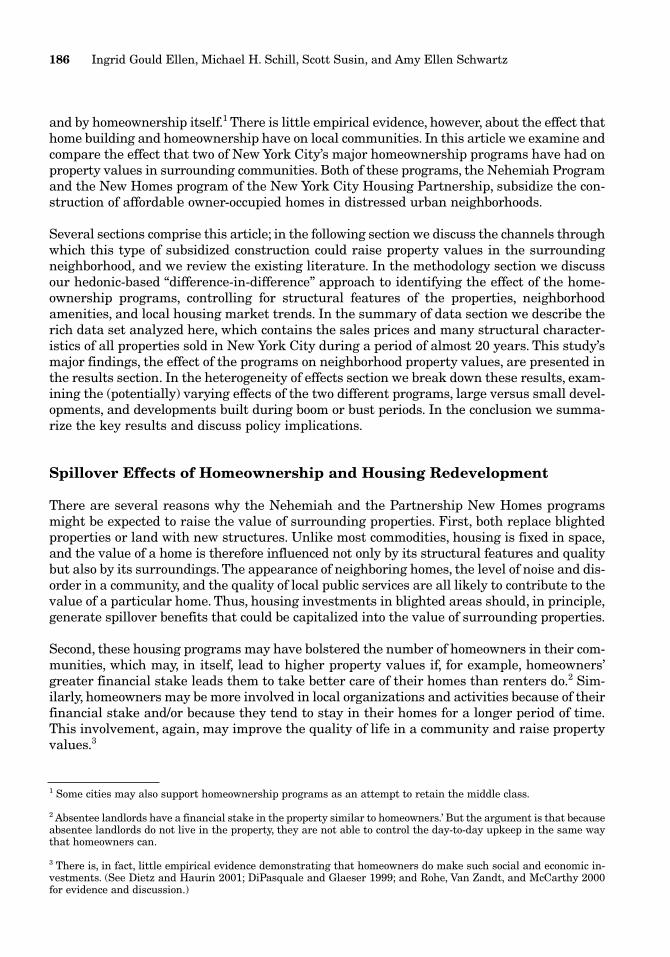
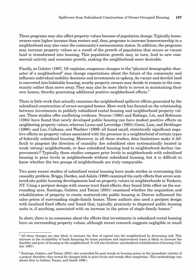
Third, HPD has provided us with data on the precise location (down to the block level) of allhousing built through the Nehemiah and Partnership programs. Figure 1 shows the locationof these projects in the City. As shown, most of the projects have been built in Brooklyn and theBronx. We used geographic information systems techniques to measure the distance fromeach sale in our database to each Nehemiah and Partnership site and to create rings of a givendistance around each project.26 To give a sense of these rings, figure 2 shows an example ofa Partnership development located on the Brooklyn/Queens border, and the development’ssurrounding rings. The innermost ring extends 500 feet (usually one to two blocks) from theproject, the second ring extends 1,000 feet (one to four blocks), and the outermost ring extends2,000 feet (three to eight blocks).
Spillovers from Subsidized Construction of Owner-Occupied Housing 195
apartments tend to be rare in the 34 community districts that have Nehemiah or Partnership New Homes devel-opments. We should also note that most of the apartment buildings in our sample are rent stabilized. Given that,typically, legally allowable rents are above market rents outside affluent neighborhoods in Manhattan and Brook-lyn, we do not think that their inclusion biases our results (see Pollakowski 1997).
24 This area includes 3 community districts in Manhattan, 9 in the Bronx, 12 in Brooklyn, 9 in Queens, and 1 in Stat-en Island.
25 Note that most of the RPAD data used in this study were collected in 1999. It is conceivable that some of thebuilding characteristics may have changed between the time of sale and 1999; however, most of the characteristicsthat we use in the hedonic regressions are fairly immutable (e.g., corner location, square feet, presence of a garage).Furthermore, to examine whether the building characteristics tend to remain constant over time, we merged RPADdata from 1990 and 1999 and found that for 8 of the 10 variables examined, the characteristic remained unchangedin 97 percent or more of the cases. “Year built” and “number of units” remained unchanged in only 87 and 93 percentof the cases, respectively. We suspect that the majority of these changes are corrections, rather than true changes,because these characteristics change very rarely. Thus, the 1999 RPAD file may actually be a better estimate of1990 characteristics than is the 1990 file. The abandonment variable was collected in 1980.
26 Because all buildings in New York City have been geocoded by the New York City Department of City Planning,we used a “crosswalk” (the “geosupport file”) that associates each tax lot with an x, y coordinate (that is, latitude, lon-gitude using the U.S. State Plane 1927 projection), community district, and census tract. Usually, a tax lot is a build-ing and is an identifier available to the homes sales and RPAD data. We were able to assign x, y coordinates and othergeographic variables to more than 98 percent of the sales using this method. For the Nehemiah and Partnershipdata, only the tax block on which the property is located (which corresponds to a physical block) is available. Aftercollapsing the geosupport file to the tax block level (i.e., calculating the center of each block), we were able to assignan x, y coordinate to 99.7 percent of these projects.
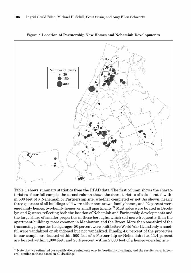
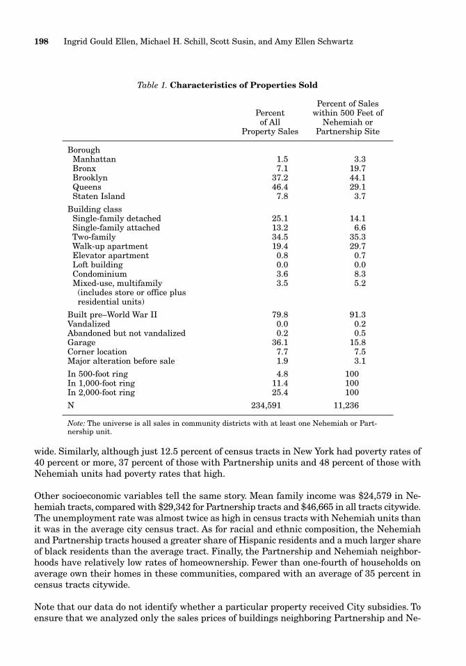
Table 1 shows summary statistics from the RPAD data. The first column shows the charac-teristics of our full sample; the second column shows the characteristics of sales located with-in 500 feet of a Nehemiah or Partnership site, whether completed or not. As shown, nearlythree-quarters of all buildings sold were either one- or two-family homes, and 92 percent wereone-family homes, two-family homes, or small apartments.27 Most sales were located in Brook-lyn and Queens, reflecting both the location of Nehemiah and Partnership developments andthe large share of smaller properties in these boroughs, which sell more frequently than theapartment buildings more common in Manhattan and the Bronx. More than one-third of thetransacting properties had garages, 80 percent were built before World War II, and only a hand-ful were vandalized or abandoned but not vandalized. Finally, 4.8 percent of the propertiesin our sample are located within 500 feet of a Partnership or Nehemiah site, 11.4 percentare located within 1,000 feet, and 25.4 percent within 2,000 feet of a homeownership site.
196 Ingrid Gould Ellen, Michael H. Schill, Scott Susin, and Amy Ellen Schwartz
Figure 1. Location of Partnership New Homes and Nehemiah Developments
Number of Units30150
300
27 Note that we estimated our specifications using only one- to four-family dwellings, and the results were, in gen-eral, similar to those based on all dwellings.

The data reveal some systematic differences between properties that are located close to Ne-hemiah or Partnership sites and those that are not. Because of the location of these develop-ments, properties that fall in the 500-foot ring are much more likely to be in Brooklyn, Man-hattan, or the Bronx. They are also much older, less likely to be single-family homes, morelikely to be walk-ups, and much less likely to have garages than properties that are not closeto the developments.
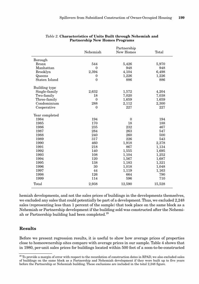
Table 2, which deals with the Nehemiah and Partnership units themselves, indicates that12,468 of the 15,528 units built (80 percent) are in Brooklyn or the Bronx and more than 13,000(85 percent) were completed during the 1990s. As for building type, 90 percent of the Ne-hemiah units are single-family homes, compared with just 12 percent of the Partnership units,which are more likely to be two- and three-family homes.
Table 3 compares the average 1990 characteristics of census tracts that include Nehemiah andPartnership units in 1998 to all tracts in the City.28 Notice that 2,938 Nehemiah units werebuilt across 25 census tracts, averaging 118 units per tract; Partnership units were more dis-persed—12,590 units were built across 179 tracts, averaging 70 per tract.
This table confirms that these projects were located in distressed neighborhoods and suggeststhat neighborhoods in which Nehemiah units have been located are somewhat more disad-vantaged. For example, the average poverty rate in a tract with Nehemiah or Partnershipunits was 40.1 and 32.5 percent, respectively, compared with just 18.4 percent for tracts city-
Spillovers from Subsidized Construction of Owner-Occupied Housing 197
Figure 2. Partnership Development on Brooklyn/Queens Border
500 ft.
1,000 ft.
2,000 ft. ZIP code boundary
Park
28 The census tract data are taken from the 1990 census. Tracts are characterized as including Nehemiah or Part-nership projects even if these projects were not built until later in the decade.
wide. Similarly, although just 12.5 percent of census tracts in New York had poverty rates of40 percent or more, 37 percent of those with Partnership units and 48 percent of those withNehemiah units had poverty rates that high.
Other socioeconomic variables tell the same story. Mean family income was $24,579 in Ne-hemiah tracts, compared with $29,342 for Partnership tracts and $46,665 in all tracts citywide.The unemployment rate was almost twice as high in census tracts with Nehemiah units thanit was in the average city census tract. As for racial and ethnic composition, the Nehemiahand Partnership tracts housed a greater share of Hispanic residents and a much larger shareof black residents than the average tract. Finally, the Partnership and Nehemiah neighbor-hoods have relatively low rates of homeownership. Fewer than one-fourth of households onaverage own their homes in these communities, compared with an average of 35 percent incensus tracts citywide.
Note that our data do not identify whether a particular property received City subsidies. Toensure that we analyzed only the sales prices of buildings neighboring Partnership and Ne-
198 Ingrid Gould Ellen, Michael H. Schill, Scott Susin, and Amy Ellen Schwartz
Table 1. Characteristics of Properties Sold
Percent of SalesPercent within 500 Feet ofof All Nehemiah or
Property Sales Partnership Site
BoroughManhattan 1.5 3.3Bronx 7.1 19.7Brooklyn 37.2 44.1Queens 46.4 29.1Staten Island 7.8 3.7
Building classSingle-family detached 25.1 14.1Single-family attached 13.2 6.6Two-family 34.5 35.3Walk-up apartment 19.4 29.7Elevator apartment 0.8 0.7Loft building 0.0 0.0Condominium 3.6 8.3Mixed-use, multifamily 3.5 5.2
(includes store or office plus residential units)
Built pre–World War II 79.8 91.3Vandalized 0.0 0.2Abandoned but not vandalized 0.2 0.5Garage 36.1 15.8Corner location 7.7 7.5Major alteration before sale 1.9 3.1
In 500-foot ring 4.8 100In 1,000-foot ring 11.4 100In 2,000-foot ring 25.4 100
N 234,591 11,236
Note: The universe is all sales in community districts with at least one Nehemiah or Part-nership unit.
hemiah developments, and not the sales prices of buildings in the developments themselves,we excluded any sales that could potentially be part of a development.Thus, we excluded 2,248sales (representing less than 1 percent of the sample) that took place on the same block as aNehemiah or Partnership development if the building sold was constructed after the Nehemi-ah or Partnership building had been completed.29
Results
Before we present regression results, it is useful to show how average prices of propertiesclose to homeownership sites compare with average prices in our sample. Table 4 shows thatin 1980, per-unit sales prices for buildings located within 500 feet of a soon-to-be-constructed
Spillovers from Subsidized Construction of Owner-Occupied Housing 199
Table 2. Characteristics of Units Built through Nehemiah andPartnership New Homes Programs
PartnershipNehemiah New Homes Total
BoroughBronx 544 5,426 5,970Manhattan 0 948 948Brooklyn 2,394 4,104 6,498Queens 0 1,226 1,226Staten Island 0 886 886
Building typeSingle-family 2,632 1,572 4,204Two-family 18 7,020 7,038Three-family 0 1,659 1,659Condominium 288 2,112 2,300Cooperative 0 227 227
Year completed1984 194 0 1941985 170 18 1881986 235 232 4671987 284 263 5471988 240 260 5001989 317 226 5431990 460 1,918 2,3781991 218 867 1,1341992 140 1,555 1,6951993 108 1,104 1,2521994 120 1,567 1,6871995 138 1,183 1,3211996 30 1,018 1,0481997 44 1,119 1,1631998 126 664 7901999 114 596 710
Total 2,938 12,590 15,528
29 To provide a margin of error with respect to the recordation of construction dates in RPAD, we also excluded salesof buildings on the same block as a Partnership and Nehemiah development if they were built up to five yearsbefore the Partnership or Nehemiah building. These exclusions are included in the total 2,248 figure.

Nehemiah or Partnership site were on average 43 percent lower than the prices of all build-ings located in the 34 community districts; prices in the 1,000-foot ring were 34.9 percent lower,and prices in the 2,000-foot ring were 27.6 percent lower.
Clearly, these projects were located in neighborhoods with depressed housing prices.30 Yet,the table also shows that over time, the differential has fallen. By 1999, prices of propertiessold within 500 feet of a Nehemiah or Partnership site were on average only 23.8 percent lowerthan the mean price in our overall sample.
The real question, of course, is whether the construction of Partnership and Nehemiah proj-ects in these rings contributes to that relative price rise in the rings. To isolate the influenceof proximity to a completed homeownership project, we estimate the regressions discussedabove, in which the dependent variable is the log of the sales price per unit, and which con-trol for building and local neighborhood characteristics and include a full complement of ZIPcode and quarter interaction effects (ZIP code–quarter fixed effects).
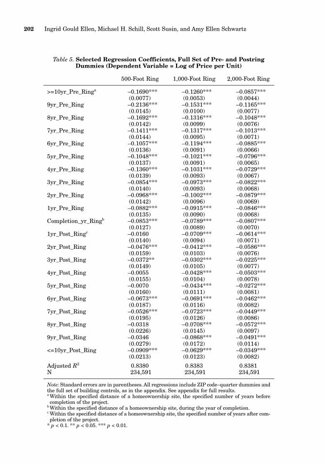
Table 5 reports the estimated regression coefficients for ring variables and their standard er-rors. Other variables in the regressions include age and its square; log of square footage; num-ber of buildings on the same lot; dummy variables indicating whether the property was on thecorner, had been vandalized, was of an odd shape, or included a garage; and 18 building clas-sification variables such as two-family home or single-family detached. Overall, the model per-forms well—structural variables have the expected signs and the regressions explain morethan 83 percent of the variation in log prices.31 (See table A.1 in the appendix for the full setof parameter estimates.)
200 Ingrid Gould Ellen, Michael H. Schill, Scott Susin, and Amy Ellen Schwartz
Table 3. 1990 Characteristics of Partnership and Nehemiah Census Tracts
Tracts with Tracts with All Tracts inNehemiah Units Partnership Units New York City
Mean poverty rate 40.1% 32.5% 18.4%Percent of tracts with 48.0% 37.4% 12.5%
poverty rate >= 40%Mean percentage of 33.0% 27.3% 13.8%
households on public assistance
Mean family income $24,579 $29,342 $46,665Mean unemployment rate 18.5% 14.8% 9.7%Mean percentage of adult 23.4% 27.0% 39.7%
residents with some college education
Mean percentage black 72.0% 51.5% 28.9%Mean percentage Hispanic 32.3% 39.3% 21.9%Mean homeownership rate 20.1% 24.2% 34.8%
N 25 179 2,131
30 Given the evidence shown in table 3 that the census tracts surrounding Nehemiah and Partnership sites arenotably less affluent than those in the city at large, it is no doubt true that prices in the rings surrounding these sitesare even lower in comparison with average prices in all community districts.
31 Briefly, results indicate that sales price is higher if a building is larger or newer, located on a corner, or includes agarage. Sales price is lower if the building is vandalized or abandoned but not vandalized. The building class dum-

Turning to the ring dummies, recall that the coefficients can be interpreted as the percentagedifference between the price of properties within the rings and comparable properties locatedoutside the rings but in the same ZIP code. First, note that all coefficients are negative andmost are statistically significant. Consistent with the uncontrolled results in table 4, parame-ter estimates indicate that prices of properties located in the rings tend to be lower than pricesof comparable properties located in the ZIP code, both before and after project completion. Notethat the estimated price differential between properties inside and outside the ring are con-siderably smaller than the uncontrolled price differentials shown in table 4. Once we controlfor quality, the price differentials diminish, suggesting that properties in the rings are of loweraverage quality than those outside. Second, in general, coefficients become smaller overtime. Thus, prices in the rings rise over time relative to prices in their surrounding ZIP code,
Spillovers from Subsidized Construction of Owner-Occupied Housing 201
Table 4. Percentage Difference between Average Housing Pricesin Rings and Average Annual Price, by Year
Prices in Prices in Prices inAverage per 500-Foot 1,000-Foot 2,000-FootUnit Price in Ring Relative Ring Relative Ring Relative
34 Community to Sample to Sample to SampleYear Districts ($) Mean (%) Mean (%) Mean (%)
1980 54,571 –43.4 –34.9 –27.61981 53,547 –43.1 –37.1 –29.11982 55,783 –35.9 –34.0 –30.31983 63,354 –45.8 –42.0 –33.51984 70,231 –50.0 –43.4 –34.91985 82,308 –50.5 –46.9 –39.31986 105,596 –53.8 –48.5 –39.91987 127,636 –52.0 –46.5 –39.01988 136,673 –48.7 –42.1 –34.81989 138,454 –42.6 –36.9 –29.71990 134,520 –42.2 –35.4 –29.81991 128,339 –40.5 –37.4 –30.71992 119,691 –36.6 –33.4 –28.91993 115,792 –35.0 –32.5 –27.51994 115,769 –28.3 –29.2 –24.31995 112,795 –26.0 –24.3 –21.91996 107,245 –32.8 –28.6 –23.11997 107,807 –30.3 –25.7 –21.41998 111,482 –26.7 –23.9 –21.51999 116,413 –23.8 –18.0 –17.1
Note: This table is based on the coefficients of simple bivariate regressions that regresslogarithm of price on year in the given geographic area and are not adjusted for othercovariates. Prices reported in 1999 dollars.
mies are also consistent with expectations. Sales prices per unit for most of the building types are lower than thosefor single-family attached homes (the omitted category). Somewhat surprisingly, the coefficient on the dummy vari-able indicating that the building has undergone a major alteration before sale is negative, which may reflect the gen-erally worse shape of buildings that have undergone such major alterations, in ways that are not captured by our data.Statistically significant coefficients on dummy variables indicating missing values for the age or size of a buildingindicate that the buildings missing age data are less valuable than others (perhaps because they are older), and build-ings missing square-footage data are more valuable (perhaps because they are larger). However, condominiumsmissing square-footage data (representing 90 percent of the sales missing square-footage data) appear to be some-what smaller. In total, just over 1 percent of property sales were missing square-footage data, and 3 percent were miss-ing age data.
202 Ingrid Gould Ellen, Michael H. Schill, Scott Susin, and Amy Ellen Schwartz
Table 5. Selected Regression Coefficients, Full Set of Pre- and PostringDummies (Dependent Variable = Log of Price per Unit)
500-Foot Ring 1,000-Foot Ring 2,000-Foot Ring
>=10yr_Pre_Ringa –0.1690*** –0.1260*** –0.0857***(0.0077) (0.0053) (0.0044)
9yr_Pre_Ring –0.2136*** –0.1531*** –0.1165***(0.0145) (0.0100) (0.0077)
8yr_Pre_Ring –0.1692*** –0.1316*** –0.1048***(0.0142) (0.0099) (0.0076)
7yr_Pre_Ring –0.1411*** –0.1317*** –0.1013***(0.0144) (0.0095) (0.0071)
6yr_Pre_Ring –0.1057*** –0.1194*** –0.0885***(0.0136) (0.0091) (0.0066)
5yr_Pre_Ring –0.1048*** –0.1021*** –0.0796***(0.0137) (0.0091) (0.0065)
4yr_Pre_Ring –0.1360*** –0.1031*** –0.0729***(0.0139) (0.0093) (0.0067)
3yr_Pre_Ring –0.0854*** –0.0973*** –0.0822***(0.0140) (0.0093) (0.0068)
2yr_Pre_Ring –0.0968*** –0.1002*** –0.0879***(0.0142) (0.0096) (0.0069)
1yr_Pre_Ring –0.0882*** –0.0915*** –0.0846***(0.0135) (0.0090) (0.0068)
Completion_yr_Ringb –0.0853*** –0.0789*** –0.0807***(0.0127) (0.0089) (0.0070)
1yr_Post_Ringc –0.0160 –0.0709*** –0.0614***(0.0140) (0.0094) (0.0071)
2yr_Post_Ring –0.0476*** –0.0412*** –0.0586***(0.0159) (0.0103) (0.0076)
3yr_Post_Ring –0.0372** –0.0302*** –0.0225***(0.0149) (0.0105) (0.0077)
4yr_Post_Ring –0.0055 –0.0428*** –0.0503***(0.0155) (0.0104) (0.0078)
5yr_Post_Ring –0.0070 –0.0434*** –0.0272***(0.0160) (0.0111) (0.0081)
6yr_Post_Ring –0.0673*** –0.0691*** –0.0462***(0.0187) (0.0116) (0.0082)
7yr_Post_Ring –0.0526*** –0.0723*** –0.0449***(0.0195) (0.0126) (0.0086)
8yr_Post_Ring –0.0318 –0.0708*** –0.0572***(0.0226) (0.0145) (0.0097)
9yr_Post_Ring –0.0346 –0.0868*** –0.0491***(0.0279) (0.0172) (0.0114)
<=10yr_Post_Ring –0.0909*** –0.0629*** –0.0349***(0.0213) (0.0123) (0.0082)
Adjusted R2 0.8380 0.8383 0.8381N 234,591 234,591 234,591
Note: Standard errors are in parentheses. All regressions include ZIP code–quarter dummies andthe full set of building controls, as in the appendix. See appendix for full results.a Within the specified distance of a homeownership site, the specified number of years beforecompletion of the project.
b Within the specified distance of a homeownership site, during the year of completion.c Within the specified distance of a homeownership site, the specified number of years after com-pletion of the project.
* p < 0.1. ** p < 0.05. *** p < 0.01.
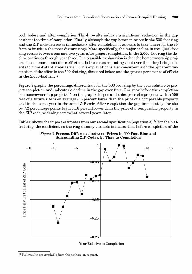
both before and after completion. Third, results indicate a significant reduction in the gapat about the time of completion. Finally, although the gap between prices in the 500-foot ringand the ZIP code decreases immediately after completion, it appears to take longer for the ef-fects to be felt in the more distant rings. More specifically, the major decline in the 1,000-footring occurs between one and two years after project completion. In the 2,000-foot ring the de-cline continues through year three. One plausible explanation is that the homeownership proj-ects have a more immediate effect on their close surroundings, but over time they bring ben-efits to more distant areas as well. (This explanation is also consistent with the apparent dis-sipation of the effect in the 500-foot ring, discussed below, and the greater persistence of effectsin the 2,000-foot ring.)
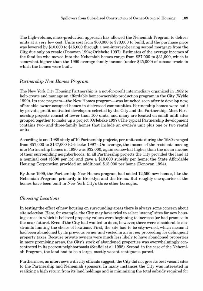
Figure 3 graphs the percentage differentials for the 500-foot ring by the year relative to pro-ject completion and indicates a decline in the gap over time. One year before the completionof a homeownership project (–1 on the graph) the per-unit sales price of a property within 500feet of a future site is on average 8.8 percent lower than the price of a comparable propertysold in the same year in the same ZIP code. After completion the gap immediately shrinksby 7.2 percentage points to just 1.6 percent lower than the price of a comparable property inthe ZIP code, widening somewhat several years later.
Table 6 shows the impact estimates from our second specification (equation 3).32 For the 500-foot ring, the coefficient on the ring dummy variable indicates that before completion of the
Spillovers from Subsidized Construction of Owner-Occupied Housing 203
Figure 3. Percent Difference between Prices in 500-Foot Ring andSurrounding ZIP Codes, by Time to Completion
–0.25
–0.20
–0.15
–0.10
–0.05
0–15 –10 –5 0 5 10 15
Year Relative to Completion
Pri
ce R
elat
ive
to R
est
of Z
IP C
ode
32 Full results are available from the authors on request.
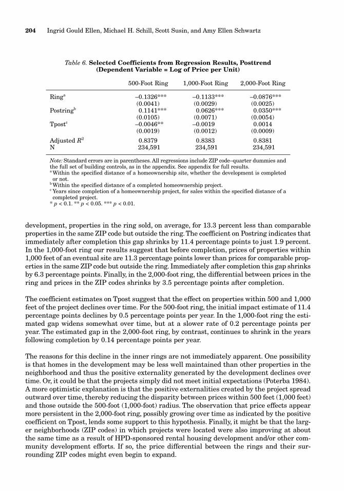
development, properties in the ring sold, on average, for 13.3 percent less than comparableproperties in the same ZIP code but outside the ring. The coefficient on Postring indicates thatimmediately after completion this gap shrinks by 11.4 percentage points to just 1.9 percent.In the 1,000-foot ring our results suggest that before completion, prices of properties within1,000 feet of an eventual site are 11.3 percentage points lower than prices for comparable prop-erties in the same ZIP code but outside the ring. Immediately after completion this gap shrinksby 6.3 percentage points. Finally, in the 2,000-foot ring, the differential between prices in thering and prices in the ZIP codes shrinks by 3.5 percentage points after completion.
The coefficient estimates on Tpost suggest that the effect on properties within 500 and 1,000feet of the project declines over time. For the 500-foot ring, the initial impact estimate of 11.4percentage points declines by 0.5 percentage points per year. In the 1,000-foot ring the esti-mated gap widens somewhat over time, but at a slower rate of 0.2 percentage points peryear. The estimated gap in the 2,000-foot ring, by contrast, continues to shrink in the yearsfollowing completion by 0.14 percentage points per year.
The reasons for this decline in the inner rings are not immediately apparent. One possibilityis that homes in the development may be less well maintained than other properties in theneighborhood and thus the positive externality generated by the development declines overtime. Or, it could be that the projects simply did not meet initial expectations (Poterba 1984).A more optimistic explanation is that the positive externalities created by the project spreadoutward over time, thereby reducing the disparity between prices within 500 feet (1,000 feet)and those outside the 500-foot (1,000-foot) radius. The observation that price effects appearmore persistent in the 2,000-foot ring, possibly growing over time as indicated by the positivecoefficient on Tpost, lends some support to this hypothesis. Finally, it might be that the larg-er neighborhoods (ZIP codes) in which projects were located were also improving at aboutthe same time as a result of HPD-sponsored rental housing development and/or other com-munity development efforts. If so, the price differential between the rings and their sur-rounding ZIP codes might even begin to expand.
204 Ingrid Gould Ellen, Michael H. Schill, Scott Susin, and Amy Ellen Schwartz
Table 6. Selected Coefficients from Regression Results, Posttrend(Dependent Variable = Log of Price per Unit)
500-Foot Ring 1,000-Foot Ring 2,000-Foot Ring
Ringa –0.1326*** –0.1133*** –0.0876***(0.0041) (0.0029) (0.0025)
Postringb 0.1141*** 0.0626*** 0.0350***(0.0105) (0.0071) (0.0054)
Tpostc –0.0046** –0.0019 0.0014(0.0019) (0.0012) (0.0009)
Adjusted R2 0.8379 0.8383 0.8381N 234,591 234,591 234,591
Note: Standard errors are in parentheses. All regressions include ZIP code–quarter dummies andthe full set of building controls, as in the appendix. See appendix for full results.a Within the specified distance of a homeownership site, whether the development is completedor not.
b Within the specified distance of a completed homeownership project.c Years since completion of a homeownership project, for sales within the specified distance of acompleted project.
* p < 0.1. ** p < 0.05. *** p < 0.01.
As noted above and as shown in figure 3, the average price differential between the rings andtheir ZIP codes was already declining before project completion. Even without the homeown-ership projects, the differential might have continued to decline. Our third specification pro-vides an estimate of impact above and beyond what would have been predicted by previoustrends in prices in the ring–ZIP code price gap (see equation 4). As noted, essentially theseimpact estimates reflect the assumption that prices in the rings would have continued to riseat the same rate relative to the ZIP code as they had been in the previous five years.
As shown in table 7, results suggest that immediately after completion the gap between pricesin the 500-foot rings and their surrounding ZIP codes falls by an average of 6.4 percentagepoints. A similar pattern obtains in the 1,000-foot and 2,000-foot rings, though changes arepredictably smaller. After completion the gap between prices in the 1,000-foot ring and pricesin the larger ZIP code is shown to shrink by 3.3 percentage points, and the gap between the2,000-foot ring and the ZIP code falls by 2.9 percentage points.33
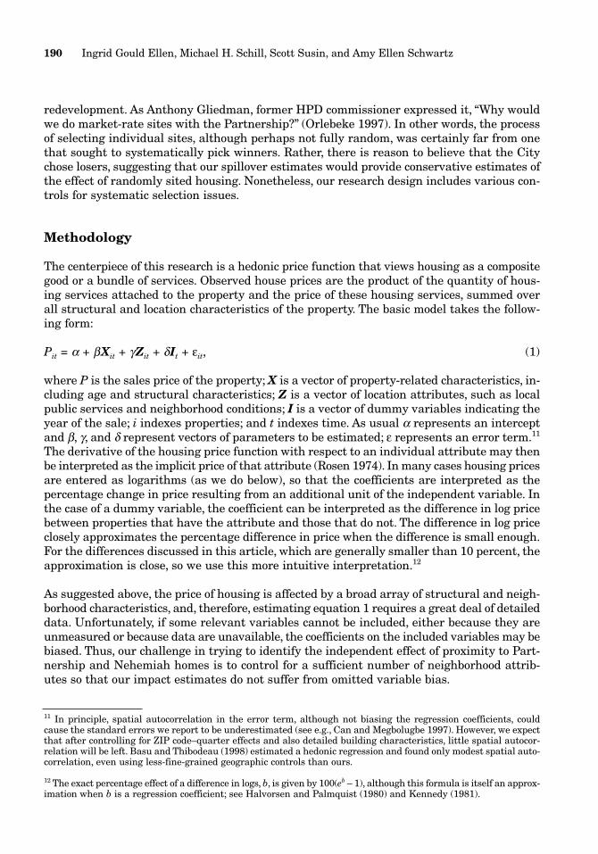
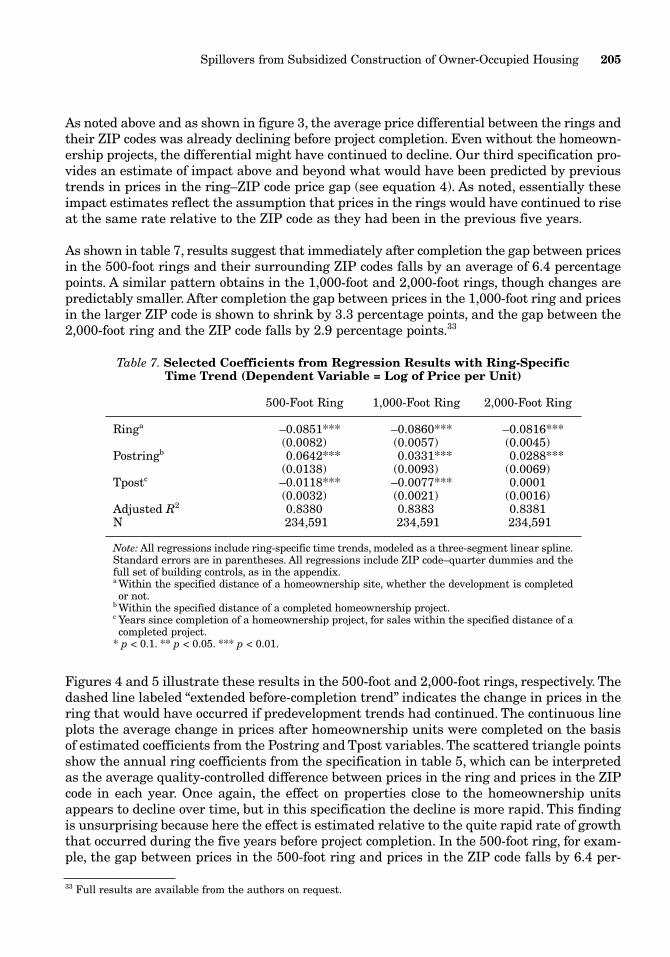
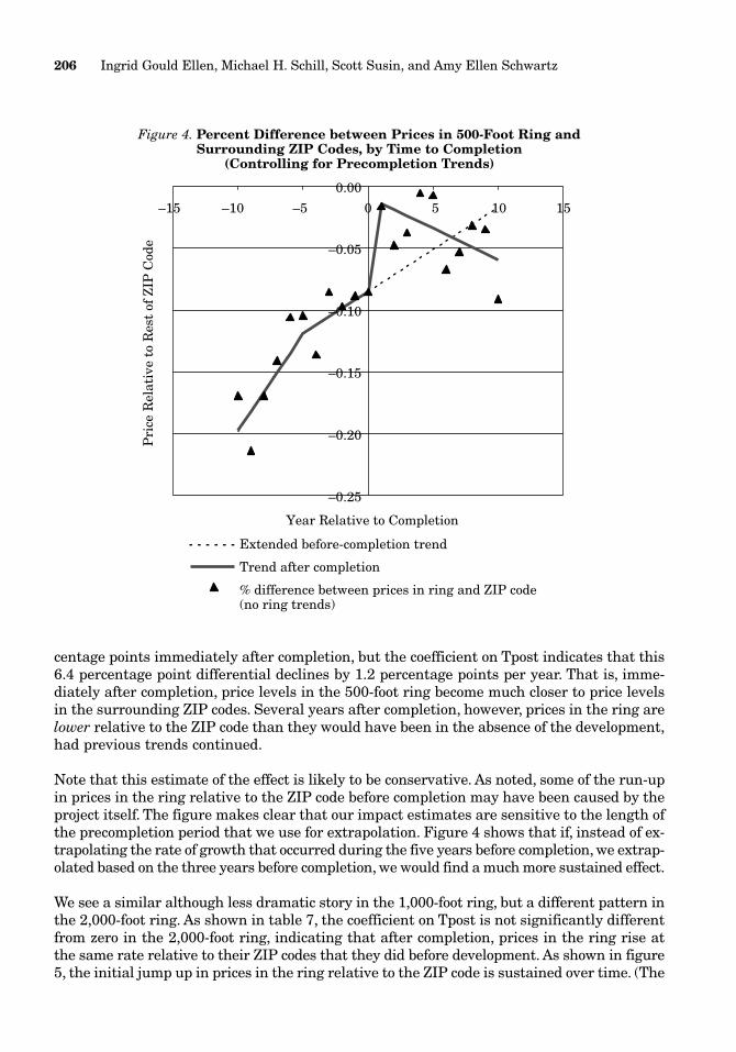
Figures 4 and 5 illustrate these results in the 500-foot and 2,000-foot rings, respectively. Thedashed line labeled “extended before-completion trend” indicates the change in prices in thering that would have occurred if predevelopment trends had continued. The continuous lineplots the average change in prices after homeownership units were completed on the basisof estimated coefficients from the Postring and Tpost variables. The scattered triangle pointsshow the annual ring coefficients from the specification in table 5, which can be interpretedas the average quality-controlled difference between prices in the ring and prices in the ZIPcode in each year. Once again, the effect on properties close to the homeownership unitsappears to decline over time, but in this specification the decline is more rapid. This findingis unsurprising because here the effect is estimated relative to the quite rapid rate of growththat occurred during the five years before project completion. In the 500-foot ring, for exam-ple, the gap between prices in the 500-foot ring and prices in the ZIP code falls by 6.4 per-
Spillovers from Subsidized Construction of Owner-Occupied Housing 205
33 Full results are available from the authors on request.
Table 7. Selected Coefficients from Regression Results with Ring-SpecificTime Trend (Dependent Variable = Log of Price per Unit)
500-Foot Ring 1,000-Foot Ring 2,000-Foot Ring
Ringa –0.0851*** –0.0860*** –0.0816***(0.0082) (0.0057) (0.0045)
Postringb 0.0642*** 0.0331*** 0.0288***(0.0138) (0.0093) (0.0069)
Tpostc –0.0118*** –0.0077*** 0.0001(0.0032) (0.0021) (0.0016)
Adjusted R2 0.8380 0.8383 0.8381N 234,591 234,591 234,591
Note: All regressions include ring-specific time trends, modeled as a three-segment linear spline.Standard errors are in parentheses. All regressions include ZIP code–quarter dummies and thefull set of building controls, as in the appendix.a Within the specified distance of a homeownership site, whether the development is completedor not.
b Within the specified distance of a completed homeownership project.c Years since completion of a homeownership project, for sales within the specified distance of acompleted project.
* p < 0.1. ** p < 0.05. *** p < 0.01.
centage points immediately after completion, but the coefficient on Tpost indicates that this6.4 percentage point differential declines by 1.2 percentage points per year. That is, imme-diately after completion, price levels in the 500-foot ring become much closer to price levelsin the surrounding ZIP codes. Several years after completion, however, prices in the ring arelower relative to the ZIP code than they would have been in the absence of the development,had previous trends continued.
Note that this estimate of the effect is likely to be conservative. As noted, some of the run-upin prices in the ring relative to the ZIP code before completion may have been caused by theproject itself. The figure makes clear that our impact estimates are sensitive to the length ofthe precompletion period that we use for extrapolation. Figure 4 shows that if, instead of ex-trapolating the rate of growth that occurred during the five years before completion, we extrap-olated based on the three years before completion, we would find a much more sustained effect.
We see a similar although less dramatic story in the 1,000-foot ring, but a different pattern inthe 2,000-foot ring. As shown in table 7, the coefficient on Tpost is not significantly differentfrom zero in the 2,000-foot ring, indicating that after completion, prices in the ring rise atthe same rate relative to their ZIP codes that they did before development. As shown in figure5, the initial jump up in prices in the ring relative to the ZIP code is sustained over time. (The
206 Ingrid Gould Ellen, Michael H. Schill, Scott Susin, and Amy Ellen Schwartz
Figure 4. Percent Difference between Prices in 500-Foot Ring andSurrounding ZIP Codes, by Time to Completion
(Controlling for Precompletion Trends)
–15 –10 –5 0 5 10 15
–0.25
–0.20
–0.15
–0.10
–0.05
0.00
Year Relative to Completion
Pri
ce R
elat
ive
to R
est
of Z
IP C
ode
Extended before-completion trend
Trend after completion
% difference between prices in ring and ZIP code(no ring trends)

gap between the extended before-completion trend and the trend after completion is constant.)Again, this pattern may reflect a spread over time of spillover effects of the new housing unitsto larger areas.
Heterogeneity of Effects
In this section we explore potential differences across three sources of heterogeneity: projectsize (number of units), project type (Nehemiah vs. Partnership), and timing (i.e., housing mar-ket conditions). We do so by supplementing the model in equation 4 with variables captur-ing size, type, and housing market conditions.
Number of Units
The notion that effects depend on project size has broad intuitive appeal. It seems reasonable,for instance, to assume that the effect of 300 units will be greater than the effect of a singleunit. In table 8 we examine the role of the scale, testing whether there are different effects forproperties in the ring of 1 to 50 units, 51 to 100 units, 101 to 200 units, 201 to 400 units, and
Spillovers from Subsidized Construction of Owner-Occupied Housing 207
Figure 5. Percent Difference between Prices in 2,000-Foot Ringand Surrounding ZIP Codes, by Time to Completion
(Controlling for Precompletion Trends)
–0.20
–0.15
–0.10
–0.05
0.00
0.05–15 –10 –5 0 5 10 15
Year Relative to Completion
Pri
ce R
elat
ive
to R
est
of Z
IP C
ode
Extended before-completion trend
Trend after completion
% difference between prices in ring and ZIP code (no ring trends)

401+ units.34 (In the 500-foot ring the latter three categories are collapsed into one; in the1,000-foot ring the latter two categories are collapsed into one.)
In the 500-foot ring, larger scale indeed appears to imply significantly larger effects. The gapbetween the prices of properties in the ring and properties in the ZIP code falls by 3.8 per-centage points after 50 or fewer homeownership units are completed, by 9.5 percentage pointsafter 51 to 100 units are completed, and by nearly 19 percentage points after more than 100units are completed.
208 Ingrid Gould Ellen, Michael H. Schill, Scott Susin, and Amy Ellen Schwartz
34 We experimented with several different ways to represent project size. We tested a linear model, and the coeffi-cient on the number of units was consistently positive. A quadratic specification yielded less consistent results, butin all rings the coefficient on the quadratic term was positive and statistically significant in the 500- and 2,000-footrings. Note that we do not distinguish between a sale that is within a certain distance of two 50-unit developmentsand another sale that is within the same distance of a single 100-unit development. Our specification controls justfor the total number of units within a certain distance.
Table 8. Selected Coefficients from Regression Results withRing-Specific Time Trend, Controlling for Project Size
(Dependent Variable = Log of Price per Unit)
500-Foot Ring 1,000-Foot Ring 2,000-Foot Ring
Ringa –0.0845*** –0.0870*** –0.0834***(0.0082) (0.0057) (0.0045)
Postring, 1–50 unitsb 0.0380** 0.0333*** 0.0475***(0.0151) (0.0104) (0.0079)
Postring, 51–100 units 0.0953*** 0.0115 0.0100(0.0234) (0.0159) (0.0114)
Postring, 101–200 units 0.1890*** 0.0284 –0.0121(0.0319) (0.0177) (0.0121)
Postring, 201–400 units .— 0.1006*** –0.0618***(0.0311) (0.0168)
Postring, 401+ units .— .— 0.0484*(0.0263)
Tpost, 1–50 unitsc –0.0071** –0.0041* 0.0007(0.0035) (0.0023) (0.0018)
Tpost, 51–100 units –0.0231*** –0.0093*** 0.0046**(0.0048) (0.0032) (0.0022)
Tpost, 101–200 units –0.0218*** –0.0124*** 0.0057**(0.0060) (0.0035) (0.0024)
Tpost, 201–400 units .— –0.0170*** 0.0045(0.0050) (0.0029)
Tpost, 401+ units .— .— –0.0078**(0.0037)
Adjusted R2 0.8389 0.8392 0.8390N 234,591 234,591 234,591
Note: All regressions include ring-specific time trends. Standard errors are in parentheses. All re-gressions include ZIP code–quarter dummies and the full set of building controls, as in theappendix.a Within the specified distance of a homeownership site, whether the development is completedor not.
b Within the specified distance of a completed homeownership project of the specified size.c Years since completion of a homeownership project, for sales within the specified distance of acompleted project of the specified size.
* p < 0.1. ** p < 0.05. *** p < 0.01.
In the 1,000-foot and 2,000-foot rings, estimated effects inside the ring of the largest develop-ments (more than 200 units in the 1,000-foot and more than 400 units in the 2,000-foot ring)are fairly large. At the same time, typically, the estimated effect on properties near smallernumbers of units is much smaller or, in two cases, actually negative. Interestingly, the esti-mated effect of proximity to 1 to 50 units is positive and statistically significant, whereas theeffect of proximity to 51 to 200 units is negligible.
In summary, we find that overall, larger projects have a greater effect on property values.35 Thispattern would be predicted by any of the mechanisms that would generate positive external-ities. For example, if city investments raise neighborhood property values because they removedilapidated buildings and clean up vacant lots, larger projects should result in larger improve-ments. In contrast, this pattern would not be expected if the results were driven by sampleselection bias—that is, the city’s ability to “pick winners” by choosing sites likely to appreci-ate in value. If anything, this type of bias should be most important for the smallest projectsbecause smaller tracts of land are much more readily available, giving HPD greater flexibil-ity over site selection.
Project Type
As noted previously, the Nehemiah and the Partnership New Homes programs differ in poten-tially important ways. Typically, Nehemiah developments include large numbers of identicalsingle-family row homes built on large, vacant tracts of city-owned land. Partnership develop-ments include a greater variety of housing types and often they were built on much smallerparcels. In addition, Nehemiah units were considerably less costly to build and to buy; there-fore, owner-occupants of these units have somewhat lower incomes. Thus, Partnership andNehemiah developments may well have different effects on surrounding neighborhoods.
To explore such differences we supplemented the models in table 8 with variables capturingthe proportion of Nehemiah units in each of the different size categories (1 to 50 units, 51 to100 units, 101+ units) as well as a variable identifying whether the property sold was in thering of a Nehemiah unit. Doing so allowed us to investigate the extent to which the propor-tion of Nehemiah units within a given distance of a property has an effect on the price of theproperty, after controlling for the total number of units.36
We found that before development, prices of properties within 500 feet of a future Partnershipsite were on average only 5.4 percent lower than prices of comparable properties in their ZIPcodes. As expected, properties located within 500 feet of future Nehemiah units were consid-erably more distressed, with prices on average 29.5 percent (5.4 percent plus 24.1 percent)lower than prices of comparable properties in their ZIP codes.
We find somewhat mixed evidence about whether the effects differ with project sponsor or type.In the 500-foot ring, coefficients on the Postring-Share Nehemiah interaction terms are positive
Spillovers from Subsidized Construction of Owner-Occupied Housing 209
35 Santiago, Galster, and Tatian (2001) also found that having a larger number of projects within 1,001 to 2,000 feetof a sale magnifies the initial positive effect. However, they do not find similar scale effects for projects that arewithin 1,000 feet of a sale.
36 Full results are available from the authors on request.
for the 1-to-50-unit and 101+–unit categories and, in the case of the 101+–unit category, sta-tistically significant. In particular, results suggest that being located near more than 100 com-pleted Partnership units increases the prices in the ring relative to the ZIP code by 15.8 per-centage points; the effect of being near the same number of Nehemiah units is estimated tobe a price increase of 23.6 percentage points.37 In the 1,000-foot ring, by contrast, the typeof unit has little effect on the magnitude of the effect. And in the 2,000-foot ring the effect oflarger shares of Nehemiah units appears to be negative, at least in the case of large projects.In short, it appears that Nehemiah units may have somewhat larger effects on properties thatare nearby, but the geographic reach of their effect appears to be more limited. We plan to ex-plore those differences further in future work.
Timing
The 20-year period for which we examined housing prices covers two distinct periods in NewYork City’s housing market. As shown in table 4, prices rose rapidly in our 34 community dis-tricts during the 1980s. Between 1982 and 1988, average housing prices rose by 145 percent,after controlling for inflation. That increase amounts to an average annual increase of rough-ly 16 percent in real terms. During the 1990s prices fell—albeit at a much slower rate—before rising again slowly at the very end of the decade.
It is possible that we might see different effects for these homeownership developments dur-ing these very different eras in the housing market. It may be, for example, that the privatesector was willing to develop housing in our selected set of ZIP codes during boom times butwas unwilling to do so when the housing market was less favorable. If so (and if the privatesector was effectively never willing to develop housing inside the actual rings), we might findthat Nehemiah and Partnership developments had a smaller effect during the 1980s whenhousing prices were rising so rapidly. It might also be that the housing market cycles aresomewhat different in lower-priced areas—perhaps they lag slightly behind the more afflu-ent areas. Finally, the small positive effects of these homeownership developments may sim-ply be difficult to pick up in years in which housing prices are rapidly rising.
To test for differences in differing housing markets, we separately examined the effect on salesthat took place during the 1980s and on sales that took place during the 1990s. In the interestof brevity we do not show the results here, but we found few significant differences in effects.Naturally, prices in the rings relative to the ZIP codes before completion were lower for prop-erties selling in the 1980s. (Again, as shown in table 4, prices in the rings were lower relativeto their ZIP codes during the 1980s.) But we see no significant differences in the immediateeffect of the homeownership units. The one difference is that in the 500-foot ring the initialpositive effect on prices appears to disappear almost immediately for sales in the 1980s, where-as for properties that sold during the 1990s, the positive effects appear to be more sustained.
210 Ingrid Gould Ellen, Michael H. Schill, Scott Susin, and Amy Ellen Schwartz
37 One possible explanation is that the Nehemiah developments in the 101+–unit category actually contain a largernumber of units. But that is not the case. In fact, the Partnership developments in the 101+–unit category appear tobe somewhat larger on average. For sales within 500 feet of a Nehemiah development of more than 100 units, themean number of units within 500 feet of the sale is 158. For sales within 500 feet of a Partnership development ofmore than 100 units, the mean number of units within 500 feet of the sale is 182. More generally, the mean numberof Partnership units and the mean number of Nehemiah units—in the given categories—are virtually identical.
Conclusion
With the benefit of data that are more precise than the data employed in previous studies, thisarticle provides a more detailed portrait of what happens to property values following thedevelopment of affordable owner-occupied housing. We show that prices of properties in therings surrounding the homeownership projects have risen relative to their ZIP codes duringthe past two decades, and our results suggest that part of this rise is attributable to twoaffordable homeownership programs in New York City: the Partnership New Homes pro-gram, administered by the New York City Housing Partnership, and the Nehemiah Planprograms, administered by South Bronx Churches and East Brooklyn Congregations. Thatis, these efforts appear to have had a positive effect on property values in their immediateneighborhoods.
The source of this positive externality is not clear. It may result from the transformation ofvacant or derelict eyesores into well-maintained, pleasant homes. It may also be caused bythe inmigration of relatively higher-income residents to the neighborhoods. Finally, a higherrate of homeownership in itself may generate positive effects for the community, ranging fromgreater neighborhood stability to better upkeep and more community activism.
In future work we hope to shed more light on the roots of the positive effect. In particular, wewill compare the effects that the City’s rental housing programs have on surrounding proper-ty values with the effects of homeownership programs.To the extent that owner-occupied hous-ing appears to have larger effects, this might suggest that owner-occupied housing yields uniquebenefits, above and beyond the effects of removing blight and producing pleasant and attrac-tive homes.
As for policy implications, this article suggests that owners of properties in the relevant com-munities will enjoy an increase in wealth that appears to be generated by the new housing. Inaddition, to the extent that the City reassesses properties in these communities, additionaltax revenues will be generated. Of course, higher property values may not benefit everyonefinancially. Rents may also increase in these areas to reflect the increase in value attribut-able to the homeownership programs. For low- and moderate-income households already hav-ing difficulty paying their rents, an increase in homeownership in the community may be amixed blessing.38 Part of this potential increase in rents would likely be ameliorated by theexistence of rent regulation in many of the neighborhoods in which Partnership and Nehemi-ah housing are located. Nevertheless, the question of how the improvement in property val-ues surrounding new homeownership housing units compares with the costs of the program(both in terms of the actual subsidies and possible negative effects on renters) requires sharp-er estimates and more empirical investigation. Such a cost-benefit analysis may be critical tofuture decision making.
Spillovers from Subsidized Construction of Owner-Occupied Housing 211
38 In 1999, almost one-quarter of all renters in New York City paid more than half of their income in rent (New YorkUniversity School of Law 2001).
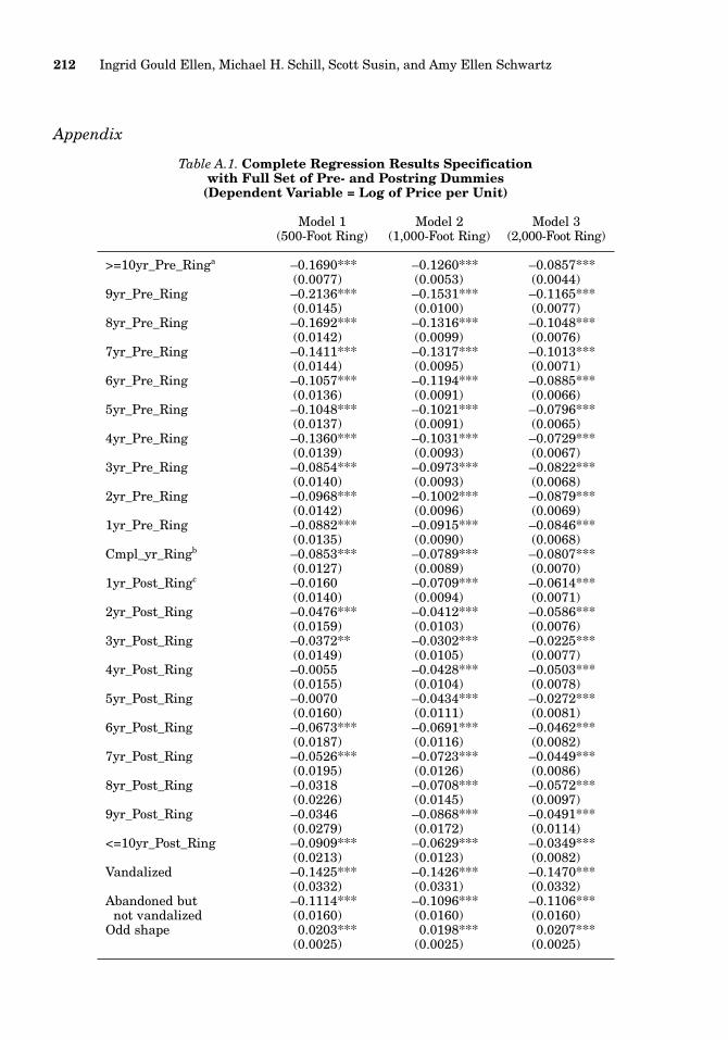
Appendix
212 Ingrid Gould Ellen, Michael H. Schill, Scott Susin, and Amy Ellen Schwartz
Table A.1. Complete Regression Results Specificationwith Full Set of Pre- and Postring Dummies
(Dependent Variable = Log of Price per Unit)
Model 1 Model 2 Model 3(500-Foot Ring) (1,000-Foot Ring) (2,000-Foot Ring)
>=10yr_Pre_Ringa –0.1690*** –0.1260*** –0.0857***(0.0077) (0.0053) (0.0044)
9yr_Pre_Ring –0.2136*** –0.1531*** –0.1165***(0.0145) (0.0100) (0.0077)
8yr_Pre_Ring –0.1692*** –0.1316*** –0.1048***(0.0142) (0.0099) (0.0076)
7yr_Pre_Ring –0.1411*** –0.1317*** –0.1013***(0.0144) (0.0095) (0.0071)
6yr_Pre_Ring –0.1057*** –0.1194*** –0.0885***(0.0136) (0.0091) (0.0066)
5yr_Pre_Ring –0.1048*** –0.1021*** –0.0796***(0.0137) (0.0091) (0.0065)
4yr_Pre_Ring –0.1360*** –0.1031*** –0.0729***(0.0139) (0.0093) (0.0067)
3yr_Pre_Ring –0.0854*** –0.0973*** –0.0822***(0.0140) (0.0093) (0.0068)
2yr_Pre_Ring –0.0968*** –0.1002*** –0.0879***(0.0142) (0.0096) (0.0069)
1yr_Pre_Ring –0.0882*** –0.0915*** –0.0846***(0.0135) (0.0090) (0.0068)
Cmpl_yr_Ringb –0.0853*** –0.0789*** –0.0807***(0.0127) (0.0089) (0.0070)
1yr_Post_Ringc –0.0160 –0.0709*** –0.0614***(0.0140) (0.0094) (0.0071)
2yr_Post_Ring –0.0476*** –0.0412*** –0.0586***(0.0159) (0.0103) (0.0076)
3yr_Post_Ring –0.0372** –0.0302*** –0.0225***(0.0149) (0.0105) (0.0077)
4yr_Post_Ring –0.0055 –0.0428*** –0.0503***(0.0155) (0.0104) (0.0078)
5yr_Post_Ring –0.0070 –0.0434*** –0.0272***(0.0160) (0.0111) (0.0081)
6yr_Post_Ring –0.0673*** –0.0691*** –0.0462***(0.0187) (0.0116) (0.0082)
7yr_Post_Ring –0.0526*** –0.0723*** –0.0449***(0.0195) (0.0126) (0.0086)
8yr_Post_Ring –0.0318 –0.0708*** –0.0572***(0.0226) (0.0145) (0.0097)
9yr_Post_Ring –0.0346 –0.0868*** –0.0491***(0.0279) (0.0172) (0.0114)
<=10yr_Post_Ring –0.0909*** –0.0629*** –0.0349***(0.0213) (0.0123) (0.0082)
Vandalized –0.1425*** –0.1426*** –0.1470***(0.0332) (0.0331) (0.0332)
Abandoned but –0.1114*** –0.1096*** –0.1106***not vandalized (0.0160) (0.0160) (0.0160)
Odd shape 0.0203*** 0.0198*** 0.0207***(0.0025) (0.0025) (0.0025)
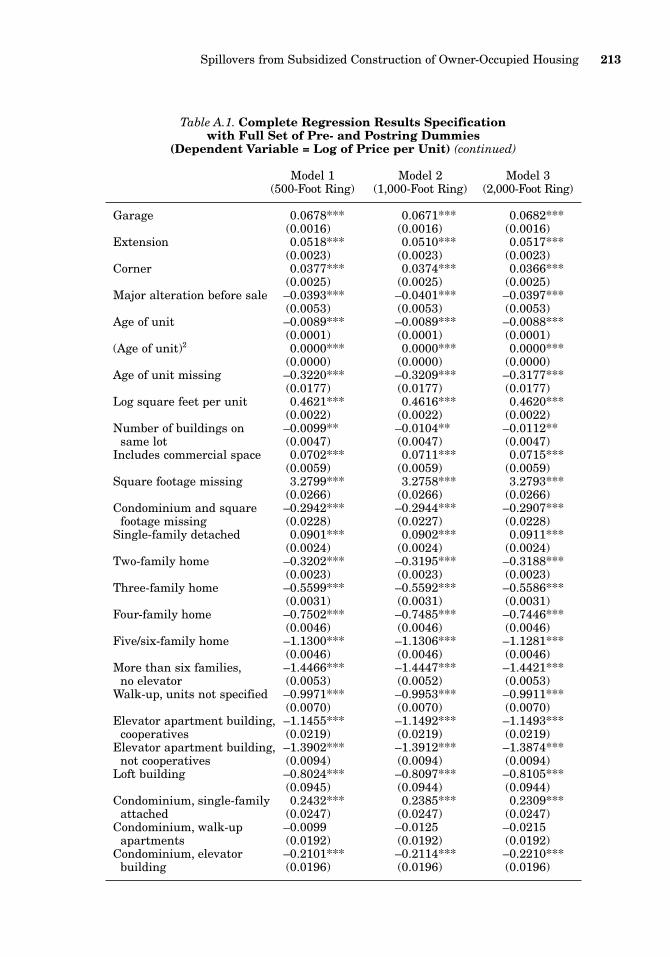
Spillovers from Subsidized Construction of Owner-Occupied Housing 213
Table A.1. Complete Regression Results Specificationwith Full Set of Pre- and Postring Dummies
(Dependent Variable = Log of Price per Unit) (continued)
Model 1 Model 2 Model 3(500-Foot Ring) (1,000-Foot Ring) (2,000-Foot Ring)
Garage 0.0678*** 0.0671*** 0.0682***(0.0016) (0.0016) (0.0016)
Extension 0.0518*** 0.0510*** 0.0517***(0.0023) (0.0023) (0.0023)
Corner 0.0377*** 0.0374*** 0.0366***(0.0025) (0.0025) (0.0025)
Major alteration before sale –0.0393*** –0.0401*** –0.0397***(0.0053) (0.0053) (0.0053)
Age of unit –0.0089*** –0.0089*** –0.0088***(0.0001) (0.0001) (0.0001)
(Age of unit)2 0.0000*** 0.0000*** 0.0000***(0.0000) (0.0000) (0.0000)
Age of unit missing –0.3220*** –0.3209*** –0.3177***(0.0177) (0.0177) (0.0177)
Log square feet per unit 0.4621*** 0.4616*** 0.4620***(0.0022) (0.0022) (0.0022)
Number of buildings on –0.0099** –0.0104** –0.0112**same lot (0.0047) (0.0047) (0.0047)
Includes commercial space 0.0702*** 0.0711*** 0.0715***(0.0059) (0.0059) (0.0059)
Square footage missing 3.2799*** 3.2758*** 3.2793***(0.0266) (0.0266) (0.0266)
Condominium and square –0.2942*** –0.2944*** –0.2907***footage missing (0.0228) (0.0227) (0.0228)
Single-family detached 0.0901*** 0.0902*** 0.0911***(0.0024) (0.0024) (0.0024)
Two-family home –0.3202*** –0.3195*** –0.3188***(0.0023) (0.0023) (0.0023)
Three-family home –0.5599*** –0.5592*** –0.5586***(0.0031) (0.0031) (0.0031)
Four-family home –0.7502*** –0.7485*** –0.7446***(0.0046) (0.0046) (0.0046)
Five/six-family home –1.1300*** –1.1306*** –1.1281***(0.0046) (0.0046) (0.0046)
More than six families, –1.4466*** –1.4447*** –1.4421***no elevator (0.0053) (0.0052) (0.0053)
Walk-up, units not specified –0.9971*** –0.9953*** –0.9911***(0.0070) (0.0070) (0.0070)
Elevator apartment building, –1.1455*** –1.1492*** –1.1493***cooperatives (0.0219) (0.0219) (0.0219)
Elevator apartment building, –1.3902*** –1.3912*** –1.3874***not cooperatives (0.0094) (0.0094) (0.0094)
Loft building –0.8024*** –0.8097*** –0.8105***(0.0945) (0.0944) (0.0944)
Condominium, single-family 0.2432*** 0.2385*** 0.2309***attached (0.0247) (0.0247) (0.0247)
Condominium, walk-up –0.0099 –0.0125 –0.0215apartments (0.0192) (0.0192) (0.0192)
Condominium, elevator –0.2101*** –0.2114*** –0.2210***building (0.0196) (0.0196) (0.0196)
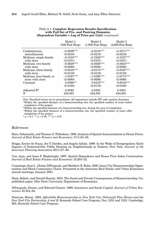
References
Basu, Sabyasachi, and Thomas G. Thibodeau. 1998. Analysis of Spatial Autocorrelation in House Prices.Journal of Real Estate Finance and Economics 17(1):61–85.
Briggs, Xavier de Souza, Joe T. Darden, and Angela Aidala. 1999. In the Wake of Desegregation: EarlyImpacts of Scattered-Site Public Housing on Neighborhoods in Yonkers, New York. Journal of theAmerican Planning Association 65(1):27–49.
Can, Ayse, and Isaac F. Megbolugbe. 1997. Spatial Dependence and House Price Index Construction.Journal of Real Estate Finance and Economics 14:203–22.
Cummings, Jean L., Denise DiPasquale, and Matthew E. Kahn. 2000. Inner City Homeownership Oppor-tunities and Black Community Choice. Presented at the American Real Estate and Urban Economicsannual meetings, January 2001.
Dietz, Robert, and Donald Haurin. 2001. The Social and Private Consequences of Homeownership. Un-published paper. Ohio State University, Department of Economics.
DiPasquale, Denise, and Edward Glaeser. 1999. Incentives and Social Capital. Journal of Urban Eco-nomics 45:354–84.
Donovan, Shaun. 1994. Affordable Homeownership in New York City: Nehemiah Plan Homes and theNew York City Partnership, A and B. Kennedy School Case Program, Nos. 1252 and 1253. Cambridge,MA: Kennedy School Case Program.
214 Ingrid Gould Ellen, Michael H. Schill, Scott Susin, and Amy Ellen Schwartz
Table A.1. Complete Regression Results Specificationwith Full Set of Pre- and Postring Dummies
(Dependent Variable = Log of Price per Unit) (continued)
Model 1 Model 2 Model 3(500-Foot Ring) (1,000-Foot Ring) (2,000-Foot Ring)
Condominium, –0.3509*** –0.3518*** –0.3571***miscellaneous (0.0218) (0.0218) (0.0218)
Multiuse, single-family –0.1518*** –0.1520*** –0.1527***with store (0.0101) (0.0101) (0.0101)
Multiuse, two-family –0.5628*** –0.5626*** –0.5624***with store (0.0080) (0.0080) (0.0080)
Multiuse, three-family –0.8218*** –0.8174*** –0.8197***with store (0.0119) (0.0119) (0.0119)
Multiuse, four-family or –1.0197*** –1.0196*** –1.0173***more with store (0.0090) (0.0090) (0.0090)
Constant 8.8390** 8.8476*** 8.8516***(0.0180) (0.0179) (0.0180)
Adjusted R2 0.8380 0.8383 0.8381N 234,591 234,591 234,591
Note: Standard errors are in parentheses. All regressions include ZIP code–quarter dummies.a Within the specified distance of a homeownership site, the specified number of years beforecompletion of the project.
b Within the specified distance of a homeownership site, during the year of completion.c Within the specified distance of a homeownership site, the specified number of years aftercompletion of the project.
* p < 0.1. ** p < 0.05. *** p < 0.01.

Galster, George C. 1987. Homeowners and Neighborhood Reinvestment. Durham, NC: Duke UniversityPress.
Galster, George C., Peter Tatian, and Robin Smith. 1999.The Impact of Neighbors Who Use Section 8 Cer-tificates on Property Values. Housing Policy Debate 10(4):879–917.
Goetz, Edward, Hin Kin Lam, and Anne Heitlinger. 1996. There Goes the Neighborhood? The Impact ofSubsidized Multi-Family Housing on Urban Neighborhoods. Working Paper No. 96-1. Center for Urbanand Regional Affairs.
Halvorsen, Robert, and Raymond Palmquist. 1980. The Interpretation of Dummy Variables in Semilog-arithmic Equations. American Economic Review 70(3):474–75.
Kennedy, Peter E. 1981. Estimation with Correctly Interpreted Dummy Variables in SemilogarithmicEquations. American Economic Review 71(4):801.
Lee, Chang-Moo, Dennis P. Culhane, and Susan M. Wachter. 1999. The Differential Impacts of FederallyAssisted Housing Programs on Nearby Property Values: A Philadelphia Case Study. Housing Policy De-bate 10(1):75–93.
Lyons, Robert F., and Scott Loveridge. 1993. A Hedonic Estimation of the Effect of Federally SubsidizedHousing on Nearby Residential Property Values. Staff Paper No. P93-6. St. Paul, MN: University of Min-nesota, Department of Agriculture and Applied Economics.
New York University School of Law, Center For Real Estate and Urban Policy. 2001. The State of theCity’s Housing and Neighborhoods. New York.
Nourse, Hugh O. 1963. The Effects of Public Housing on Property Values in St. Louis. Land Economics39: 433–41.
Orlebeke, Charles J. 1997. New Life at Ground Zero: New York, Homeownership, and the Future ofAmerican Cities. Albany, NY: Rockefeller Institute Press.
Pollakowski, Henry O. 1997. The Effects of Rent Deregulation in New York City. Working Paper No. 67.Cambridge, MA: Massachusetts Institute of Technology, Center for Real Estate.
Poterba, James M. 1984. Tax Subsidies to Owner-Occupied Housing: An Asset Market Approach. Quar-terly Journal of Economics 99(4):729–52.
Rabiega, William A., Ta-Win Lin, and Linda Robinson. 1984. The Property Value Impacts of Public Hous-ing Projects in Low and Moderate Density Residential Neighborhoods. Land Economics 60:174–79.
Rohe, William, and Leslie Stewart. 1996. Homeownership and Neighborhood Stability. Housing PolicyDebate 7(1):37–81.
Rohe, William, Shannon Van Zandt, and George McCarthy. 2000. The Social Benefits and Costs of Home-ownership: A Critical Assessment of the Research. Working Paper No. 00-01. Washington, DC: ResearchInstitute for Housing America.
Rosen, Sherwin. 1974. Hedonic Prices and Implicit Markets: Product Differentiation in Pure Competi-tion. Journal of Political Economy 82(1):34–55.
Santiago, Anna M., George C. Galster, and Peter Tatian. 2001. Assessing the Property Value Impactsof the Dispersed Subsidy Housing Program in Denver. Journal of Policy Analysis and Management 20(1):65–88.
Scafidi, Benjamin P., Michael H. Schill, Susan M. Wachter, and Dennis P. Culhane. 1998. An EconomicAnalysis of Housing Abandonment. Journal of Housing Economics 7(4):287–303.
Spillovers from Subsidized Construction of Owner-Occupied Housing 215

Stuart, Lee. 1997. Come, Let Us Rebuild the Walls of Jerusalem: Broad-Based Organizing in the SouthBronx. In Signs of Hope in the City: Ministries of Community Renewal, ed. Robert D. Carle and LouisA Decaro Jr., 129–39. Valley Forge, PA: Judson.
Wylde, Kathryn. 1999. The Contribution of Public-Private Partnerships to New York’s Assisted HousingIndustry. In Housing and Community Development in New York City, ed. Michael H. Schill, 73–91.Albany,NY: SUNY Press.
216 Ingrid Gould Ellen, Michael H. Schill, Scott Susin, and Amy Ellen Schwartz