Building Edge-Failure Resilient Networks∗

C. Chekuri† A. Gupta‡ A. Kumar§ J. Naor ¶ D. Raz ¶

January 3, 2005

Abstract

We consider the design of resilient networks that are fault tolerant against link failures.

Resilience against link failures can be built into the network by providing backup paths, which

are used in the eventuality of an edge failure occurring on a primary path in the network. We

consider several network design problems in this context; these problems are motivated by the

requirements of current high speed optical networks. In all the following problems, the objective

is to provide resilience in networks while minimizing the cost incurred.

The main problem under consideration in this paper is that of backup allocation: this problem

takes as its input an already provisioned primary network and a parameter k, and allocates

backup capacity on the edges of the underlying network so that all the demand can be routed

even in the presence of k edge failures. We also consider a variant of this problem where the

primary network has a tree topology, and it is required that the restored network retains a tree

topology.

We then address the problem of simultaneous primary and backup allocation: we are given

specifications of the traffic to be handled, and the goal is to provision both the primary as

well as the backup network. Finally, we investigate a single commodity problem motivated by a

pragmatic scenario in which the primary network is not known in advance and demands between

source-sink pairs arrive online.

Key words: network design, link failure, backup path, restoration, approximation algorithm.

∗An extended abstract of this work appeared in the Proceedings of the 9th Integer Programming and Combinatorial

Optimization Conference, Cambridge Massachusetts, 2002. Much of this work was done while the authors were at

Lucent Bell Labs, 600 Mountain Avenue, Murray Hill NJ 07974.†Contact author. Bell Labs, Lucent Technologies, 600-700 Mountain Avenue, Murray Hill, NJ 07974.

chekuri@research.bell-labs.com. Ph: +1-908-582-1204. Fax: +1-908-582-5857.‡Dept. of Computer Science, Carnegie Mellon University, Pittsburgh PA 15213. anupamg@cs.cmu.edu.§Department of Computer Science, Indian Institute of Technology, Hauz Khas, New Delhi, India - 110016.

amitk@cse.iitd.ernet.in. This research was partly done while the author was at Cornell University where he

was supported in part by an ONR Young Investigator Award of Jon Kleinberg.¶Computer Science Department, Technion, Israel Institute of Technology, Haifa 32000, Israel.

naor,danny@cs.technion.ac.il. This research is supported in part by a US-Israel BSF Grant 2002276,

and by a foundational and strategical research grant from the Israeli Ministry of Science.

1

1 Introduction

Fault tolerance in networks is an important and well studied topic with many applications. Tele-

phone networks and other proprietary networks adopt a variety of techniques to provide reliability

and resilience to network failures and have been in use for many years now. On the other hand

data networks such as the Internet have very little centralized fault tolerance. Instead, the network

relies on the routing protocols that adapt to failures by sending traffic on alternate paths. This

has been acceptable till now, since there have been no guarantees on the quality of service on the

Internet. However, with the maturity of the Internet, an increasing number of applications now

require quality of service guarantees. The emergence of very high capacity optical networks has

enabled the move towards providing users with their own virtual private networks or VPNs [32].

Several virtual networks can be accommodated on the underlying (high capacity) optical network

by splitting the available bandwidth among them. However, since VPNs also require us to pro-

vide QoS guarantees to applications and users, fault tolerance and network resilience become very

critical issues: failure of a single high capacity link can disrupt all the VPNs that use that link.

In many cases, the sheer speed and the large capacity of the links does not permit us to rely

merely on the routing protocols (say, OSPF or BGP) to successfully reroute the traffic on alternate

routes after the failure; it is now imperative to a priori provision the network to handle failures.

This places two broad constraints on these networks: 1) resources for re-routing traffic should be

reserved at the same time the sub-networks are provisioned, and 2) the routing protocol should be

simple, both for the regular routing and when a fault occurs. (See, e.g., [34] and [14] for similar

survivability issues of IP over optical networks, and [24] and [25] for discussions of fast restoration

of the MPLS tunnels that are often used to implement VPNs in optical networks [10].)

In light of the importance of the problem, there has been some recent interest in obtaining al-

gorithmic solutions for problems of guaranteeing resilience against failures. A variety of failure

and recovery models have been proposed, and it is not feasible to give even an overview of all the

models and their intricacies; the interested reader is referred to Section 1.2 for some pointers to

related work in the literature. At a high level, this paper focuses on the cases where it is guaranteed

that no more than a fixed number of edge-failures can occur, and the algorithm must provision a

minimum-cost network to allow for “local” restoration. We will expand on these assumptions in

the following paragraphs; a formal specification of the model is provided in Section 1.1.

Our model of edge-failures is adversarial; we make the assumption that there is some fixed value

k such that only k edge failures can happen in the network at any given instant of time. This

should be contrasted with probabilistic models, where edges are allowed to fail with some specified

probabilities. This assumption is commonly used in practice and seems to work reasonably well

[27]. Another pragmatic reason for this assumption is that most networks are k-connected for some

small k, and hence they cannot tolerate more than k adversarial edge failures. Furthermore, it is

interesting to note that the resulting optimization problems are already hard for the case of k = 1.

In the following discussion, we will usually restrict our attention to the single edge failure case of

k = 1; where appropriate, we will indicate how the ideas for k = 1 extend to general k. Note that

for k ≥ 2, both primary edges as well as backup edges are allowed to fail.

Resilience against single edge failures can be built into the network by providing for each edge e, a

1

backup path P (e), which is used when the edge e fails. However, since only one edge is guaranteed

to fail, making the backup paths for two different edges intersect each other and share the same

amount of bandwidth results in backup networks of lower cost. This multiplexing is one of the

factors that makes this problem especially difficult; we shall spell out some of the others as we

explain the models and our results.

In all our models we will assume that we are provisioning bandwidth on a given uncapacitated

underlying network, called the base network. In other words, we assume that there is unlimited

capacity on each edge of the base network; for each edge e, there is an associated cost of ce per

unit of bandwidth, and we can allocate any amount xe of bandwidth on it by paying ce xe. This

assumption is clearly not true for any practical network, but we make it for two reasons. First,

we believe it to be a reasonable approximation since the capacities of the underlying network are

usually much larger than the capacity of any single VPN that is to be provisioned. Second, the

capacitated versions of the problems are provably much harder, and we believe that the domain

in which they are hard does not apply to real settings. For example, the disjoint paths problem

is notoriously hard for small capacities, but it is much easier if the capacities of the edges are

sufficiently large compared to the individual demands. Similar assumptions have often been made

in the literature; see, e.g., [7, 12, 22].

We consider several network design problems with the above assumptions. The first general problem

we consider is that of Backup Allocation. In this problem, we are given an already provisioned

(primary) network, and we want to reserve backup capacity on the edges of the base network so

that traffic can be routed in the primary network even in the case of an edge failure. At this point,

we would like to point out the final requirement of the network: the restoration has to be handled

locally; i.e., if edge e = (i, j) carrying u(e) bandwidth fails, there must be a single path P (e) in the

backup network between i and j with capacity at least u(e), which stands in for the edge e.

Local restoration is important for timing guarantees. Global or end-to-end restoration could require

portions of the network far away from the end points of e to be aware of a failure at e. Another

advantage of local restoration is simplicity of the recovery mechanism. It is imperative for our

purposes that there is a single path between u and v that routes all of u(e); merely having a backup

network that is able to push the right amount of “flow” is not sufficient. This is necessary in optical

networks, where splitting the traffic is not feasible. As an aside, this local restoration can be very

easily implemented using MPLS, and is sketched in Section 1.1.1. The reader curious about MPLS

and the details of the mechanisms used for efficient local restoration of paths, can refer to the

relevant literature [10, 28, 29].

The second problem we consider is that of simultaneous Primary and Backup Allocation. We

look at both offline and online settings of the problem. In the offline case, we are given specifications

of the traffic to be handled, and we want to provision both the primary network as well as the backup

network. In the online version of the problem, demands arrive one by one. On the arrival of a pair

of terminals s, t, we must find both a primary path and a backup path between them. Again,

the online algorithm endeavors to multiplex as many backup paths as possible, and models this

by allowing different costs for an edge depending on whether it is a part of a primary or a backup

path.

Details of these problems are given in the next section. Though these problems have some sim-

2

ilarities to traditional network design problems, they also differ in some salient respects. Our

contributions include providing formal models and building upon existing techniques to give algo-

rithms for these new problems. We hope that our techniques and ideas will be useful in related

contexts.

1.1 Models and results

We now give detailed and precise formulations of the problems studied and results obtained in this

paper. In all these problems, we look at undirected base networks G = (V,E) with edge costs ceper unit bandwidth. Recall that this is an uncapacitated network, and any amount of bandwidth

xe may be allocated on e at cost ce xe.

Backup Allocation: In backup allocation, we are given an already provisioned primary network

Gp = (V p, Ep), with each edge e ∈ Ep having provisioned capacity up(e); we are also given an

upper bound k on the number of edge failures. The objective is to find an edge set Eb ⊆ E and

backup capacities ub for these edges, so that given any set F ⊆ Ep∪Eb of failed edges with |F | ≤ k,

for each edge e = (u, v) ∈ F ∩ Ep, there is a path PF (e) ∈ Eb \ F between u and v. This path

PF (e) can be used to locally restore e lest the set F fails.

5

1 2

5

5

2 22

(b)(a)

5

2

4

55

5

5

5

2

4

5

6

6

41 2

2

5

6

3

9

9

Figure 1: Backup Allocation: backup network indicated in dashed lines. (a) Backup network canhandle k = 2 edge failures only in the primary network. (b) Backup network can handle k = 2 edgefailures either in primary or the backup networks.

Of course, the backup network must have enough capacity, and given any edge e′ ∈ Eb, the total

capacity used by the paths in PF (e) | e ∈ F ∩ Ep is less than ub(e′). I.e., for all e′ ∈ Eb and

F ⊆ Ep ∪ Eb s.t |F | ≤ k,

∑

e:e∈F∩Ep,e′∈PF (e)

up(e) ≤ ub(e′).

For an example, see Figure 1; the solid lines are the primary network (with the capacities indicated),

and the dotted lines are one possible backup for it. (We do not require that the set of edges in

3

backup and primary networks be disjoint, and Eb ∩ Ep could certainly be non-empty.) Also note

that in our model both backup and primary edges can fail. In Figure 1, (a) would not be a valid

solution in our model, since some of the vertices on the cycle induced by the primary edges have

only one backup edge adjacent to them. If, for such a vertex, both a primary edge and the backup

edge adjacent to it fail, then the connection cannot be restored.

In Section 3, we describe an O(1) approximation algorithm for the backup problem when k = 1.

When then extend this to give an O(k) approximation algorithm for k > 1. We first examine the

uniform capacity case, i.e., when up(e) = 1 for all e ∈ Ep. This special case is similar to the Steiner

network problem [17, 23, 33] where the goal is to design a minimum cost network with prescribed

connectivity requirements for vertex pairs; the uniform capacity case has an additional constraint.

In Section 2 we describe an algorithm to handle this uniform capacity case. In Section 3, we extend

the algorithm to handle non-uniform capacities via capacity scaling.

Primary and Backup Allocation: In this problem, we have to build both the primary network

as well as the backup network. We require the specifications of the traffic that the primary network

should be able to carry. A common model for specifying traffic requirement is the point-to-point

demand model, where a demand matrix D = (dij) gives demands between each pair of terminals i

and j; the objective is to output the cheapest network capable of carrying the traffic specified by D.

In our setting where the base network is uncapacitated, the optimal primary network simply routes

all the flow between u and v on a shortest path between the two terminals (with the “length” of

an edge e being ce).

Considering that good estimates are often not known for the pairwise demands in real networks,

Duffield et al. [11] proposed an alternate way to specify traffic patterns, the so-called VPN hose

model. In its simplest form, each terminal i is given a threshold b(i), and a symmetric demand

matrix D = (dij) is called valid if it respects all thresholds, i.e., if∑

j dij ≤ b(i) for all i. The

primary network is specified by two quantities: a vector up indicating the bandwidth allocated on

the edges of the network, and for each pair of terminals ij a single path Pij on which their flow will

be routed. A feasible solution satisfies the following for each valid demand matrix D = (dij).

∑i<j dij χ(Pij) ≤ up. (1.1)

Here χ(P ) ∈ 0, 1|E| is the characteristic vector of a path P , and the sum is a vector sum.

Provisioning the primary network in the hose model has been studied by Gupta et al. [18], where

among other results, an optimal algorithm is given when the provisioned network is required to

be a tree; it is also shown that this tree provides a 2-approximation for the problem (without the

tree restriction). An extension of the model include the asymmetric case where both ingress and

egress thresholds bin(i) and bout(i) are given, and a demand matrix is valid if∑

j dij ≤ bout(i)

and∑

i dij ≤ bin(j); algorithms in this extended model that find near-optimal trees and general

networks are presented in [18, 20].

In this paper we study, based on the above, several models for designing primary and backup

networks. Specific details of each model are provided in the relevant sections. We obtain the

following results. We show that an α-approximation algorithm for allocating the primary network

implies an O(α log n) approximation for both primary and backup allocation. The simple two-stage

4

algorithm for this first uses the α-approximation algorithm to allocate a primary network Gp, and

then uses the algorithm of Section 3 to find a near-optimal backup network for Gp. We show that

our analysis is tight, and give examples where α = 1 but our algorithm outputs primary and backup

networks costing Ω(log n) times the optimum. Our algorithm works only for single edge failures

(k = 1).

Tree networks: It is often desirable to provision networks having a tree topology; the advantages

include simplicity, scalability and the presence of good routing schemes for trees. This prompted [18]

to give algorithms for primary allocation in the VPN hose model which outputs the optimal tree,

which they showed had cost within a factor of 2 of the optimal network. Though we can always use

the methods of Section 3 to add resilience to trees, when some edge e in a tree fails and is locally

restored by P (e), the new network may no longer be a tree. For some applications, and also for

simplicity of routing schemes, it is convenient that the network remains a tree at all times, even

after restoration.

In Section 5, we study the problem of allocating backup to a given primary network T while ensuring

that T − e+ P (e) is also a tree. We show that this problem is closely related to the group Steiner

problem on trees [16]. From this, we show that it is hard to approximate within an Ω(log2−ε n)

factor, and give a backup allocation algorithm with a pseudo-approximation guarantee of O(log2n).

The Single Commodity Problem: In practical applications, the demands often appear in an

online manner, i.e., new demands for resilient paths (i.e., primary and backup paths) between pairs

of nodes arrive one by one. We consider the case where a demand consists of a pair of vertices, the

source s and sink t, with a specified demand d to be sent between them; the goal is to construct

a primary path P and a set of backup edges Q that can be used for restoration when an edge on

P fails. As explained before, a backup edge can be used to back up several primary edges, and

hence the edges which lie on previous backup paths may have already been paid for. We model

this eventuality by allowing different primary costs and backup costs for an edge, depending on the

purpose for which we will use this edge; clearly, the primary cost of an edge should be at least as

large as the backup cost. We present a simple 2-approximation algorithm for the resulting problem.

Our 2-approximation extends to the case of protection against k-failures. We also give two natural

linear programming formulations of the problem, and show that one of these formulation dominates

the other for all instances. We point out that we are considering the local optimization problem

that needs to be solved each time a new demand arrives; our aim is not to perform the usual

competitive analysis where the online algorithm is compared to the best offline solution.

1.1.1 MPLS implementation

For the reader familiar with MPLS routing, we would like to very briefly sketch the fact that the

local restoration for the edge e = (u, v) can be very easily implemented. (Readers curious about

MPLS are referred to [10]; a theoretical model is given in [19].) Node u just precomputes the MPLS

stack Sbu,v that routes to v on the backup path P (e). (Symmetrically, the node v has a stack Sb

v,u

to route to v.) In case the edge e fails and u receives a packet desirous of taking the edge e, it could

push the stack Sbu,v onto the packet’s MPLS stack and send it on the first vertex on P (e).

5

1.2 Related Work

There have been several papers on (splittable) flow networks resilient to edge-failures; see, e.g., [7,

8, 12]. The papers [24, 25] formulate the online restoration problem as an integer program, and give

some empirical evidence in favor of their methods. The paper of [22] considers backup allocation

in the VPN hose model and gives a constant-factor approximation when accounting only for the

cost of edges not used in the primary network and hence does not provide a true approximation

algorithm. Further, [22] assumes that the primary network is a tree and hence the algorithm

does not generalize to arbitrary networks. The paper [2] looks at the problem of limited-delay

restoration; however, it does not consider the question of bandwidth allocation and its cost.

The problem of survivable network design has also been investigated extensively (see, e.g.,[3] and

the references therein). Most of this work has been focused on obtaining strong relaxations to be

used in cutting plane methods. In fact, the linear programs we use have been studied in these

contexts, and have been found to give good empirical performance. For more details on these,

and on polyhedral results related to them, see [4, 5, 6, 9]. In contrast to most of these papers, we

focus on worst-case approximation guarantees, and our results perhaps explain the good empirical

performance of relaxations considered in the literature. Our models and assumptions also differ in

some ways from those in the literature. We are interested in local restoration, and not necessarily

in end-to-end restoration. This allows our results to be applicable to the VPN hose model as well,

in contrast to the earlier literature, which is concerned primarily with the point-to-point model. We

also focus on path restoration as opposed to flow restoration. On the other hand, we do consider

a simpler model and limit ourselves only to the case of uncapacitated networks.

1.3 Paper Organization

The rest of the paper loosely follows the structure of the introduction: in Section 2, we define and

study the Constrained Steiner Network Problem, giving a constant-factor approximation for

the problem. This algorithm is crucially used in the algorithm for Backup Allocation presented

in Section 3. We then go on to the problem of simultaneous Primary and Backup Allocation in

Section 4, for which we give an O(logn) approximation algorithm. Section 5 is devoted to the

case of Backup Provisioning on tree topologies (where the restored network must also be a tree).

Finally, we conclude with the single commodity backup problem in Section 6.

Throughout the paper we use OPT to denote the value of an optimal solution to the problem being

discussed.

2 Constrained Steiner Network Problem

Given a primary network Gp = (V p, Ep) in the Backup allocation problem with k = 1, the objective

is to reserve capacity on a set of edges Eb and specify paths P (e) ⊆ Eb for each edge e ∈ Ep such

that the backup path P (e) must not contain e itself; furthermore, (1.1) requires that the capacity

of any edge on P (e) must be at least up(e).

Consider a further simplification of the problem where up(e) = 1 for all e ∈ Ep; the problem is

now to find a minimum cost set of edges Eb which, for each e = (u, v) ∈ Ep, contains a path

6

P (e) ⊆ Eb \ e between the endpoints u and v of e.

Dropping yet another constraint, we can attempt to find a minimum cost set of edges E ′ which,

for all e = (u, v) ∈ Ep, contains a path P (e) ⊆ Eb between the u and v. (Note that now P (e)

may be just the edge e itself.) This turns out to be a special case of a well studied network design

problem, the Steiner Network Design problem (SND). Formally, an instance of SND is given by an

undirected graph G = (V,E), a cost function c : E → R+, and requirements rij ∈ Z

+ for pairs of

vertices (i, j) ∈ V . (We can assume that rij = 0 for pairs (i, j) for which there is no requirement.)

The goal is to select a minimum cost set of edges E ′ ⊆ E such that there are rij edge-disjoint paths

between i and j in E ′. A 2-approximation for this problem was given by Jain [23].

We now define the Constrained Steiner Network Design problem, or the CSND problem, as the

SND problem with the added constraint that rij edge-disjoint paths in E ′ between i and j must

not contain the edge (i, j). (Note that (i, j) could still lie in E ′ and be used to connect some other

pair (i′, j′).) The k = 1, up = 1 case of the Backup allocation problem now just corresponds to

setting rij = 1 ⇐⇒ i, j ∈ Ep.

2.1 An Approximation Algorithm for CSND

We show that an α-approximation algorithm for SND can be used to obtain a 2α-approximation

algorithm for CSND. The algorithm is simple and is given below.

• Let I1 be the instance of SND with requirement r on G. Solve I1 approximately, and let E ′

be the set of edges chosen.

• Define a new requirement function r′ as follows. For (i, j) ∈ E ′ such that rij > 0, set

r′ij = rij + 1, else set r′ij = rij .

• Let I2 be the instance of SND on G with requirement function r′ and with the cost of edges

in E′ reduced to zero. Let E ′′ be an approximate solution to I2. Output E′′ ∪ E′.

It is easy to see that the above algorithm produces a feasible solution. Indeed, if (i, j) 6∈ E ′ then

E′−(i, j) contains rij edge-disjoint paths between i and j. If (i, j) ∈ E ′ then E′′ contains rij +1

edge-disjoint paths between (i, j), and hence E ′′ − (i, j) contains rij edge-disjoint paths.

Lemma 2.1 The cost of the solution to CSND produced by the above algorithm is at most 2α OPT,

where α is the approximation ratio of the algorithm used to solve SND.

Proof: It is easy to see that OPT(I1) ≤ OPT, and hence c(E ′) ≤ αOPT. We claim that

OPT(I2) ≤ OPT. Indeed, if A ⊆ E is an optimal solution to I, then A ∪ E ′ is feasible for

requirements r′. Therefore, c(E ′′ − E′) ≤ αOPT(I2) ≤ αOPT, and c(E ′′ ∪ E′) ≤ 2αOPT. 2

Using the 2-approximation algorithm for SND due to Jain [23] gives us the following corollary.

Corollary 2.2 There is a 4-approximation algorithm for the CSND problem.

In Section 3, we will build on this algorithm to give approximation algorithms for the general

Backup allocation problem.

7

2.2 Integrality Gap of an LP Relaxation for CSND

While our algorithm for CSND used the algorithm for SND as a black box, it will be useful for us to

write down a natural linear programming (LP) relaxation of the CSND problem, and consider its

integrality gap. This will be useful in Section 4. Consider the following integer linear programming

formulation for CSND, where xe is the indicator variable for picking edge e in the solution. For

compactness we use the following notation to describe the constraints. We say that a function x on

the edges supports a flow of f between s and t if the maximum flow between s and t in the graph

with capacities on the edges given by x is at least f . This property can be easily modeled by linear

constraints.

min∑

e cexe (IP1)

s.t. x supports rij flow between (i, j) in E − (i, j) for all i, j

xe ∈ 0, 1 for all e ∈ E

We relax the integrality constraints to obtain the following linear program

min∑

e cexe (LP1)

s.t. x supports rij flow between (i, j) in E − (i, j) for all i, j

xe ∈ [0, 1] for all e ∈ E

Lemma 2.3 The integrality gap of (LP1) for CSND is upper bounded by 4.

Proof: Consider the following LP formulation (LP-flow) for SND.

min∑

e cexe (LP-flow)

s.t. x supports rij flow between (i, j) in E for all i, j

xe ∈ [0, 1] for all e ∈ E

Jain’s result in [23] shows that the integrality gap of (LP-flow) is at most 2 for SND. Note that

the optimal solution to (LP-flow) for either of the instances I1 and I2 created in our algorithm

for CSND costs no more than an optimal solution to (LP1) for I; indeed, the solution to (LP1)

for I is a feasible solution to both those LPs. This, combined with the fact that (LP-flow) has an

integrality gap of at most 2, gives us the claimed result. 2

3 Backup Allocation

We now use the algorithm for CSND from Section 2 to show an O(k) approximation for the problem

of computing the cheapest backup network for a given primary network. Let G = (V,E) be the

underlying base network, and Gp = (V p, Ep) be the primary network. We are also given the primary

edge capacities up : Ep → R+. Our goal is to find an edge set Eb ⊆ E (the backup edges), and

a function ub : Eb → R+ (the backup bandwidth), and backup paths P (e) for every edge e ∈ Ep

satisfying (1.1) for any set of at most k edge failures F p.

We first state the quality of approximation we can obtain for the uniform capacity problem.

8

Lemma 3.1 For the uniform capacity backup allocation problem with k failures, there is a 4k-

approximation algorithm.

Proof: By scaling capacities we can assume without loss of generality that the primary capacity

of each edge is 1. We solve the CSND problem induced by the backup problem: for each edge (i, j)

in the primary network we set rij = k. The cost of the CSND problem is no more than 4 times the

value of an optimum solution to the backup problem. On each edge e in the solution to the CSND

problem we place a capacity of k. This increases the cost of the solution by a factor of k. The

total flow on any backup edge is at most k since this is the maximum number of edges that can

fail. Thus, the modified solution is feasible for the backup allocation problem. The cost is clearly

within 4k times the optimum cost. 2

Let upmax = maxe∈Ep up(e). Our algorithm for backup allocation given below is based on scaling

the capacities and solving the resulting uniform capacity problems separately.

• Let Epi = e ∈ Ep | up(e) ∈ [2i, 2i+1). For all e ∈ Ep

i , round up up(e) to 2i+1.

• For 1 ≤ i ≤ dlog upmaxe, independently backup Ep

i .

Let Ebi be the edges for backing up Ep

i and ubi be the backup bandwidth on Eb

i . Note that round-

ing up the bandwidths of Epi causes the the backup allocation problem on Ep

i to be a uniform

problem. The lemma below states that solving the problems separately does not cost much in the

approximation ratio.

Lemma 3.2 There is an approximation algorithm for the backup allocation problem with ratio 16k.

Proof: Let Er∗ be an optimal solution for backup allocation, with ur∗ being the bandwidth

allocation function on Er∗. For 0 ≤ i ≤ dlog upmaxe construct solutions Er∗

i , where e ∈ Er∗i with

capacity ur∗i (e) = 2i+1 if ur∗(e) ≥ 2i, and 0 otherwise. Clearly

∑i u

r∗i (e) ≤ 4ur∗(e) for each e, and

hence by linearity of the cost function,∑

i c(Er∗i ) ≤ 4c(Er∗). Note that Er∗

i is a feasible solution

to the CSND problem induced by the backup for Epi . Hence, for each i, using the approximation

algorithm for the uniform case for Epi as described in the proof of Lemma 3.1, we obtain a solution

of cost at most 4kc(Er∗i ). This completes the proof. 2

The ratio of 16k in Lemma 3.2 can be further improved to 4ek by randomness: instead of grouping

by powers of 2, grouping can be done by powers of e (with a randomly chosen starting point). This

technique is fairly standard by now (e.g., [26, 15]), but we give the proof for sake of completeness.

Theorem 3.3 Given a primary network, there is a 4k · e ' 10.87k-approximation for the k-failure

resilient backup allocation problem with linear edge cost functions.

Proof: We pick a real number α from the interval [1, e) randomly according to the density function

f(t) = 1t. Here e is the base of the natural logarithm. As before, Ep is the set of edges in the

primary network, and up(a) denotes the primary reservation on edge a. Now we group the edges

in the following manner. Define Epi as the set of edges in Ep for which up(a) lies in the interval

[α · ei, α · ei+1). Round up up(a) to α · ei+1 for all edges in the set Epi . As before, we independently

backup Epi for all i. Observe that the only difference from the earlier deterministic algorithm is in

how we group the edges.

9

We now compute the approximation ratio of this algorithm. We follow the proof of Lemma 3.2.

Fix an edge a. Let g(a) = i if ur∗(a) lies in the interval [α · ei, α · ei+1). Note that g(a) is a random

variable that takes one of two values, either blnur∗(a)c or blnur∗(a)c − 1. Then it can be shown

that the cost of our solution is at most 4k ·∑

a∈E α ·eg(a)+1 · e

e−1 . Here the factor 4k comes from the

approximation algorithm for the uniform bandwidth case, the term α ·eg(a)+1 comes from rounding

the reservations up, and the term ee−1 comes from the geometric sum.

Now, a routine calculation shows that the expected value of α · eg(a)+1 is (e − 1)ur∗(a). Thus, in

expectation, we get an approximation ratio of 4k · e. The algorithm can be easily derandomized

since there are O(|E|) distinct values of α that are of interest and these can be easily be enumerated.

2

3.1 Integrality Gap of an LP relaxation

We have shown an O(k) approximation for the backup allocation problem. We now analyze the

integrality gap of a natural LP relaxation for the problem and show that it is O(k log n). This will

allow us to analyze an algorithm for simultaneous allocation of primary and backup networks in the

next section. The LP formulation uses variables ye which indicate the backup bandwidth bought

on edge e. We relax the requirement that the flow uses k edge disjoint paths. A k-flow between a

pair of vertices s and t is a flow of k units from s to t such that the flow on any edge of the graph

is at most 1.

min∑

e ceye (LP3)

s.t.

y/upe supports a k-flow between (i, j) in E − e for all e ∈ Ep

ye ≥ 0

We now analyze the integrality gap. Recall the definition of Epi as the set of edges in Ep such

that up(e) ∈ [2i, 2i+1). As before we round up the bandwidth of these edges to 2i+1. Let xe(i) =

min1, ye/2i. Note that xe(i) ∈ [0, 1]. We claim the following.

Proposition 3.4 The variables xe(i) are feasible for the uniform bandwidth backup allocation LP

relaxation induced by Epi where the bandwidths are scaled to 1.

From Lemma 3.1 it follows that the integrality gap of (LP1), the LP for the uniform bandwidth

problem is at most 4k. Hence we can find a solution that backs up the edges in Epi with cost at

most 4k∑

e ceye. Since we only have to look at dlog upmaxe values of i, there is a solution that backs

up all edges in Ep with cost at most 4k log upmax

∑e ceye. We can make the upper bound on the

integrality gap O(k log n) via a simple argument. We set xe(i) = 0 if ye/2i ≤ 1/n3, otherwise we

set xe(i) = min1, (1+1/n)ye/2i. It is straightforward to argue that Proposition 3.4 still holds for

the variables xe(i) defined in this modified fashion. The cost goes up by a (1 + 1/n) factor. Each

edge e participates in the backup of at most O(log n) groups Epi , hence the overall cost is at most

O(k log n) times the LP cost. This gives us the following theorem.

Theorem 3.5 The integrality gap of (LP3) is O(kminlogn, log upmax).

10

The following theorem shows that our analysis is tight for k = 1.

Theorem 3.6 The integrality gap of (LP3) is Ω(log n) for k = 1.

Proof: We construct a graph G with the required gap as follows. The graph consists of a complete

binary tree T rooted at r with some additional edges. The cost of each edge in T is 1. The additional

edges go from leaves to the root and each of them is of cost d, where d is the depth of T . Primary

bandwidth is provisioned only on the edges of T and is given by up(e): for an edge e at depth d(e),

up(e) = 2d/2d(e). Backup bandwidth allocation defined by the following function ub(e) is feasible

for (LP3): ub(e) = 1 for each edge e that goes from a leaf to the root and ub(e) = up(e) for each

edge of T . It is easy to check that the cost of this solution is O(d2d).

We claim that any path solution to the backup of T in G has a cost of Ω(d22d). Setting d to be logn

gives the desired bound on the integrality gap. We now prove the claim. Let Ei be the edges of T at

depth i. Let ci be the minimum cost of backing up edges in Ei. We first note that∑

i ci ≤ 4OPT.

This follows from a simple scaling argument that we used in the proof of Lemma 3.2. Thus, it is

sufficient to prove that ci ≥ d2d. Let e be an edge in Ei and let Te be the subtree rooted under e.

We have that up(e) = 2d−i. The backup solution for Ei requires an edge from a leaf in Te to the

root with capacity up(e). Note that for any e, e′ ∈ Ei, the trees Te and Te′ are disjoint. Therefore

ci ≥ |Ei|d2d−i = d2d. 2

We note that the primary network in the above proof is a feasible primary network for an instance

in the point-to-point demand model as well as for an instance in the VPN hose model. Correctness

of the former is clear: every edge implicitly defines a point to point demand between its end points

of value equal to the primary bandwidth allocated to the edge. To see that the above primary

network is feasible for an instance in the VPN hose model, consider the leaves of T as demand

points, each with a bandwidth bound of 1.

3.2 Concave Capacity Costs

We have assumed till now that the cost per bandwidth on each edge is proportional to the band-

width. We now demonstrate the applicability of our ideas to the case where the cost is a concave

function of the capacity. Network design problems with concave cost functions are also referred

to as buy-at-bulk problems [30, 1]. For each edge e in G we let ce : R → R denote the concave

function that defines the cost per capacity on e. The algorithm we use is the same as the one for

linear capacities that we described above, the only difference is in the analysis and the performance

guarantee. We first claim that Lemma 3.1 is also valid for the concave cost functions. Lemma 3.2

requires a modification as given below.

Lemma 3.7 Let α be the approximation ratio for the uniform capacity backup allocation problem.

Then there is an approximation algorithm for the backup allocation problem with concave costs with

ratio O(α log upmax).

Proof: The proof is similar to that of Lemma 3.2. Let Er∗ be an optimal solution for backup allo-

cation, with ur∗ being the bandwidth allocation function on Er∗. For 1 ≤ i ≤ dlog upmaxe construct

solutions Er∗i , where e ∈ Er∗

i with capacity ur∗i (e) = 2i+1 if ur∗(e) ≥ 2i, and 0 otherwise. By con-

cavity of the cost function, ce(ur∗i (e)) ≤ 2ce(u

r∗(e)), hence∑

i ce(ur∗i (e)) ≤ 2ce(u

r∗i (e)) log ur∗

e (e).

Therefore∑

i c(Er∗i ) ≤ 2c(Er∗) log up

max. Note that Er∗i is a feasible backup for Ep

i , since every

11

edge in Er∗ of bandwidth at least 2i lies Er∗i with bandwidth 2i+1. Hence, for each i, using the

approximation algorithm for the uniform case for Epi would give us a solution with cost at most

αc(Er∗i ). Therefore the algorithm outputs a solution of cost no more than O(α log up

max). 2

From the above lemma we obtain the following.

Theorem 3.8 Given a primary network, there is an O(k log upmax)-approximation for the k-failure

resilient backup allocation problem with concave edge cost functions.

4 Simultaneous Primary and Backup Allocation

In this section we examine the problem of simultaneously building a primary network as well as the

backup network so as to minimize the overall cost. In this section we restrict ourselves to single edge

failures. We have a constant-factor approximation for backup allocation when given the primary

network. We use it in a natural way to provision both the primary and backup. We adopt the

two-phase strategy of first building the primary network, and then building a backup network for

it. If α is the approximation guarantee for the problem of building the primary network, we obtain

an O(α log n) approximation algorithm for the problem of Primary and Backup allocation. This

result applies when the primary network has to support a set of point-to-point demand matrices.

The set of point-to-point demands can be explicitly specified or implicitly specified as in the VPN

hose model.

For the two models we use to specify the primary bandwidth requirements, namely the point-to-

point demand model and the VPN hose model, we have constant-factor approximation algorithms

for building the primary network. For the point-to-point model an optimal solution is obtained by

shortest path routing and for the VPN model a constant factor approximation is given in [18]. We

thus obtain O(logn) approximations for the combined problem for these two models.

4.1 The O(log n) approximation algorithm

We analyze the two-stage approach for primary and backup allocation. Let Gp be the subgraph of

G that is chosen in this first step. We provide backup for this network using the algorithm described

in Section 3. To analyze this algorithm we use the LP relaxation (LP3) for the backup allocation

problem. In the following lemma we will be using extra capacity on the edges of provisioned

network itself. Note that this is allowed. We call a primary solution up minimal, if for any edge

e with up(e) > 0, we cannot reduce up(e) by even an arbitrarily small ε > 0 without violating the

feasibility of up. It follows that for a given minimal primary network and an edge e with up(e) > 0,

there is a demand matrix De for which e is critical; that is, reducing up(e) would imply that De

cannot be routed.

Lemma 4.1 Let up be any minimal solution to the primary problem. Let up∗ and ur∗ be the

primary and backup in some optimal solution. Then, up+up∗+ur∗ is a feasible solution for (LP3),

the LP relaxation for the backup of up.

Proof: Let e = (i, j) be such that up(e) > 0. Let De be the demand matrix for which e is critical.

Let f be a feasible multicommodity flow routing for De in up. It follows that f(e) = up(e) for

otherwise e is not critical for De. Let the flow paths that use e in a flow decomposition for f be

12

P1, P2, . . . , P` and let fi be the flow on Pi. For 1 ≤ h ≤ `, let xh and yh be the end points of Ph such

that i occurs before j in traversing Ph from xh to yh. Let G′ be the capacitated graph obtained

from G by removing e and setting capacities equal to up + up∗ + ur∗. We need to argue G′ can

support a flow of up(e) from i to j. We do this as follows. For 1 ≤ h ≤ `, we simultaneously send

fh units of flow from i to xh using a capacity of up. Let G′′ be the capacitated graph obtained from

G by removing e and setting capacities equal to up∗ + ur∗. Since the optimum solution is resilient

against single edge failures, for 1 ≤ h ≤ `, G′′ can simultaneously support a flow of fh units from

xh to yh. Since∑

h fh = f(e) = up(e), it follows that we can route a flow of up(e) from i to j in

G′. 2

Theorem 4.2 The two-stage approach yields an O(α logn) approximation to the combined primary

and backup allocation problem where α is the approximation ratio for finding the primary allocation.

Proof: Let P be the cost of the primary allocation and B the cost of backup allocation in the

two stage approach. From the approximation guarantee on finding P , we have P ≤ αOPT. From

Lemma 4.1, it follows that there is a feasible (LP3) relaxation for the backup allocation problem

of value at most P + OPT, hence at most (α + 1)OPT. From Theorem 3.5, the backup solution

we obtain is at most O(logn) times the LP value. Hence, B = O(α logn)OPT and the theorem

follows. 2

It turns out that the two-stage approach loses an Ω(log n) factor even if the first step obtains a

primary network of optimum cost; the example in the proof of Theorem 3.6 demonstrates this. We

observe that the two stage approach cannot guarantee a good approximation for the case of k edge

failures when k ≥ 2. We briefly describe an example to show this. The underlying graph G consists

of two vertices s, t with two parallel paths P1 and P2 between them. Each path has ` À k edges

on it. In addition, each edge e on the two paths has k parallel copies which we refer to as the

auxiliary edges associated with e. The auxiliary edges for every e ∈ P1 are “cheap” while the the

ones associated with every e ∈ P2 are “expensive”. However the cost of P1 itself is marginally more

than that of P2. Consider a point to point demand between s and t. In a two stage process, an

algorithm for building a primary network might choose P2 as a solution. For k ≥ 2, if k edges in P2

fail, then one of the expensive auxiliary edges on P2 will be forced to be chosen in the second stage.

An optimum solution consists of P1 and its auxiliary edges. The gap between the two solutions can

be made arbitrarily large by appropriately choosing the costs of the edges.

5 Backup for Tree Networks

In this section, we consider the case when the provisioned network T is a tree, and furthermore, it

is required that when an edge e fails, the network T − e+ P (e) also be a tree. The objective, as

before, is to minimize the cost of allocating the backup bandwidth. We prove that this problem at

least as hard as the group Steiner problem [16] on trees, which in turn is Ω(log2−ε n)-hard [21].

Theorem 5.1 The tree backup problem is at least as hard to approximate as the group Steiner

problem on trees. Hence, for any fixed ε > 0, the problem cannot be approximated to within a ratio

of Ω(log2−ε) unless NP ⊆ ZTIME(npolylog(n)).

13

Proof: The group Steiner tree problem is given by a weighted graph Gs = (Vs, Es), a root vertex

r ∈ Vs and ` subsets S1, . . . , S` of vertices. A solution consists of a subtree Ts ⊆ Gs containing the

root r which intersects every set, i.e., V (Ts) ∩ Si 6= ∅ for 1 ≤ i ≤ `. The objective is to find a tree

Ts of minimum cost. We will consider instance when Gs is restricted to be a tree. Note that in this

case, a solution can be completely specified by giving for 1 ≤ i ≤ `, a vertex vi ∈ Si.

We reduce the group Steiner problem on trees to the tree backup problem. The base network

G = (V,E) consists of Gs, and ` new vertices u1, . . . , u`. Each ui is connected to all the vertices

in Si, and also to r by an edge ei. Finally, for each edge e ∈ Es, E contains a parallel copy of the

edge e. All the edges in Es have unit cost, while the new edges have zero cost.

Let δ < 1 be some fixed constant. The primary network Gp = (V,Ep) has the tree edges Es along

with e1, . . . , e`; furthermore, we set up(e) = δ for e ∈ Es, and up(ei) = 1. Since each edge e ∈ Es

can be protected by this parallel copy at zero cost, we need only protect the edges ei. Since the

restored network is to be a tree when ei fails, this tree must be T − ei + fi, with fi being an edge

from ui to some wi ∈ Si. Hence, for 1 ≤ i ≤ `, we must reserve one unit of backup bandwidth on

the path from the vertex wi to r in T . This shows that the cost of the optimal backup is the same

as the cost of an optimal solution to the group Steiner tree problem in Gs. Thus the tree backup

problem is at least as hard as the group Steiner problem on trees which is hard to approximate to

within a factor of Ω(log2−ε n) [21, Theorem 1.1]. 2

We also give an algorithm for the tree problem when k = 1. Let T = Gp = (V p, Ep) be the primary

network, and let Eb be the backup edges, with up and ub be the primary and backup bandwidth

allocations. Let α be the approximation ratio for group Steiner problem on trees. It is known

that α = O(log2 n) [16]. Our algorithm outputs a solution to the backup problem whose cost is

O(α)∑

e ce(up(e) + ub(e)). Note that this does not yield a true O(α) approximation algorithm

since we are including the cost of the primary network in the upper bound. The algorithm and

the proof of the upper bound can be found in Section A in the appendix. We note that the proof

of Theorem 5.1 shows (by choosing ε appropriately) that the problem remains hard even if the

algorithm is allowed to compare its cost against∑

e ce(up(e) + ub(e)).

6 Single Source and Sink

In this section we consider a unit-capacity MPLS primary and backup allocation problem which

is motivated by the online problem of choosing the best primary and backup paths for demands

arriving one by one. Suppose that we are given source and destination vertices, denoted by s and t,

respectively. The goal is to simultaneously provision a primary path p from s to t and a backup set

of edges q of minimum overall cost. Since we are dealing with a single source-sink pair we can scale

the bandwidth requirement to 1, hence all edges have unit capacity, i.e., the primary and backup

edge sets are disjoint. We require that for any failure of k edges, e1, . . . , ek, (q ∪ p)− e1, . . . , ek

contains a path from s to t. We call this problem SSSPR (Single Source Sink Provisioning and

Restoration). Note that this requirement is slightly different from the backup model discussed

earlier in the paper; here, we do not insist on local restoration. The backup edges together with

the primary edges are required to provide connectivity from s to t. This problem is in the spirit

of the work of Kodialam and Lakshman [24, 25]. As explained before, we model the online nature

14

of the problem by using two different costs. Formally, there are two non-negative cost functions

associated with the edges: c1 gives the cost of an edge when used a primary edge, and c2 gives the

cost of an edge when used as a backup edge. We assume that c1(e) ≥ c2(e) for all edges e ∈ E.

Let p be a primary path from the source s to the destination t. The following procedure due to

Suurballe [31] computes a minimum cost backup set of edges for a given primary path p. The idea

is to direct the edges on the path p in the “backward” direction, i.e., from t to s and set their cost

to be zero. All other edges are replaced by two anti-symmetric arcs. The costs of the two arcs a

and a− that replace an edge e are set to c2(e). We now compute a shortest path q from s to t. It

can be shown that the edges of q that do not belong to p define a minimum cost local backup [31].

We first present a 2-approximation algorithm for the SSSPR problem for the case k = 1, and then

generalize it to arbitrary values of k. First, find a shortest path p from s to t with respect to the

c1-cost function. Then, use Suurballe’s [31] procedure to compute an optimal backup q to the path

p with respect to the c2-cost function. We show below that p and q together induce a 2-approximate

solution.

Theorem 6.1 The two stage approach yields a 2-approximation to SSSPR.

Proof: Let OPT be the cost of an optimal primary and backup solution and let P =∑

e∈p c1(e)

be the cost of p and Q =∑

e∈q c2(e) be the cost of q. It is clear that P ≤ OPT since we find

the cheapest primary path. We next argue that Q ≤ OPT. Consider Suurballe’s [31] algorithm to

find the optimum backup path for p. As described earlier, the algorithm finds a shortest path in

a directed graph obtained from G and p. The main observation here is that any primary path p′

and a q′ that backs up p′ yields a path in the directed graph created by Surballe’s procedure. We

omit the (straight forward) formal proof of this observation. In particular, the observation holds

for the set of edges of p∗ and q∗, where p∗ is an optimal primary path and q∗ is a set of edges that

backs up p∗. Surballe’s procedure finds the shortest path and therefore, Q ≤∑

e∈p∗∪q∗ c2(e) ≤∑e∈p∗ c1(e) +

∑e∈q∗ c2(e) ≤ OPT. Here we use the assumption that c2(e) ≤ c1(e) for all e. 2

Although we provide an approximation algorithm, we note that it is not known whether SSSPR is

NP-hard or not.

Extension to k failures. We note that the above algorithm can be easily extended to the case

where at most k edges can fail. First, find a shortest path p from s to t with respect to the c1-

cost function. Then, similar to Suurballe’s [31] procedure, direct the edges on the path p in the

“backward” direction, i.e., from t to s and set their cost to be zero. All other edges are replaced

by two anti-symmetric arcs. The costs of the two arcs a and a− that replace an edge e are set to

c2(e). We set the capacity of each arc to 1 and compute a minimum cost flow of k units from s

to t. Let q be the support of the flow in G. We claim that the edges of q that do not belong to p

define a minimum cost local backup which is resilient to k edge failures, since any cut separating s

from t contains at least k + 1 edges from p ∪ q.

We observe that p and q together induce a 2-approximate solution. Clearly, the cost of p is upper

bounded by the cost of an optimal solution. As in the case where k = 1, any primary path p′ and

backup q′ (resilient to k failures) define a flow of k units from s to t in the directed graph obtained

from G and p (as above). Therefore, the cost of q is also upper bounded by the cost of an optimal

15

solution, yielding that the solution computed is a 2-approximation.

In Section B of the appendix we provide two linear programming formulations for SSSPR. Although

we show that the worst case integrality gap for both formulations is 2, we nevertheless believe that

the formulations are of interest from the point of view of mathematical programming. They could

be of potential use in a branch and bound scheme to obtain good solutions in practice.

7 Conclusions

In this paper we explored models and algorithms for designing networks that are resilient to failures.

Our focus was on local restoration and on uncapacitated networks. With these two assumptions, we

were able to provide good approximation algorithms under a fairly general model. Our main result

on providing backup networks can be extended to capacitated networks, however, the algorithm

might violate the capacities by upmax. Can we obtain a constant factor approximation without

violating the capacities? Can we obtain improved algorithms for designing primary and backup

networks simultaneously? Can we obtain provably good algorithms in the end-to-end restoration

model? We leave these for future work.

Acknowledgments: We thank Rajeev Rastogi for providing us a copy of [22], and for useful

discussions. We are grateful to Bruce Shepherd for sharing his knowledge of the area with us,

his enthusiasm for our work, and for pointing out relevant literature. We thank Sudipto Guha

for discussions that led to to the integrality gap example in Section 6. We also thank one of the

anonymous reviewers for extensive comments that improved the presentation of the paper.

References

[1] B. Awerbuch and Y. Azar. Buy-at-bulk Network Design. In Proceedings of IEEE FOCS,

542–547, 1997.

[2] A. Bremler-Barr, Y. Afek, E. Cohen, H. Kaplan and M. Merritt. Restoration by Path Con-

catenation: Fast Recovery of MPLS Paths. In Proceedings of the ACM PODC ’01; also in

Proceedings of the ACM SIGMETRICS ’01 conference (2-page Poster). 2001.

[3] A. Balakrishnan, T. Magnanti, and P. Mirchandani. Network Design. Annotated Bibliographies

in Combinatorial Optimization, M. Dell’Amico, F. Maffioli, and S. Martello (eds.), John Wiley

and Sons, New York, 311-334, 1997.

[4] A. Balakrishnan, T. Magnanti, J. Sokol, and Y. Wang. Spare-Capacity Assignment For Line

Restoration Using a Single-Facility Type. In Operations Research, 50(4):617–635, 2002.

[5] A. Balakrishnan, T. Magnanti, J. Sokol, and Y. Wang. Telecommunication Link Restoration

Planning with Multiple Facility Types. In Annals of Operations Research, volume “Topological

Network Design in Telecommunications,” edited by P. Kubat and J. M. Smith, 106(1-4):127–

154, 2001.

[6] D. Bienstock and G. Muratore. Strong Inequalities for Capacitated Survivable Network Design

Problems. Math. Programming, 89:127–147, 2001.

16

[7] G. Brightwell, G. Oriolo and F. B. Shepherd. Reserving resilient capacity in a network. In

SIAM J. Disc. Math., 14(4):524–539, 2001.

[8] G. Brightwell, G. Oriolo and F. B. Shepherd. Reserving Resilient Capacity with Upper Bound

Constraints. In Networks, 41(2):87–96, 2003.

[9] G. Dahl and M. Stoer. A Cutting Plane Algorithm for Multicommodity Survivable Network

Design Problems. INFORMS Journal on Computing, 10:1-11, 1998.

[10] B. Davie and Y. Rekhter. MPLS: Technology and Applications. Morgan Kaufmann Publishers,

2000.

[11] N. Duffield, P. Goyal, A. Greenberg, P. Mishra, K. Ramakrishnan, and J. van der Merwe. A

flexible model for resource management in virtual private networks. In Proceedings of the ACM

SIGCOMM, Computer Communication Review, volume 29, pages 95–108, 1999.

[12] L. Fleischer, A. Meyerson, I. Saniee, F. B. Shepherd and A. Srinivasan. Near-optimal design

of MPλS tunnels with shared recovery. DIMACS Mini-Workshop on Quality of Service Issues

in the Internet, 2001.

[13] G. N. Frederickson and J. JaJa. Approximation algorithms for several graph augmentation

problems. SIAM J. on Computing, 10(2):270–283, 1981.

[14] A. Fumagalli and L. Valcarenghi. IP restoration vs. WDM Protection: Is there an Optimal

Choice? IEEE Network, 14(6):34-41, November/December 2000.

[15] M. Goemans and J. Kleinberg. An improved approximation ratio for the minimum latency

problem. In Proceedings of 7th ACM-SIAM SODA, pages 152–157, 1996.

[16] N. Garg, G. Konjevod, and R. Ravi. A polylogarithmic approximation algorithm for the group

Steiner tree problem. Journal of Algorithms, 37(1):66–84, 2000. (Preliminary version in: 9th

Annual ACM-SIAM Symposium on Discrete Algorithms, pages 253–259, 1998).

[17] M. Goemans, A. Goldberg, S. Plotkin, D. Shmoys, E. Tardos, and D. Williamson. Improved

approximation algorithms for network design problems. In Proceedings of the 5th Annual

ACM-SIAM Symposium on Discrete Algorithms, pages 223–232, 1994.

[18] A. Gupta, A. Kumar, J. Kleinberg, R. Rastogi, and B. Yener. Provisioning a Virtual Private

Network: A network design problem for multicommodity flow. In Proceedings of the 33rd An-

nual ACM Symposium on Theory of Computing, pages 389–398, 2001.

[19] A. Gupta, A. Kumar, and R. Rastogi. Traveling with a Pez dispenser (or, routing issues in

MPLS). In 42nd IEEE Symposium on Foundations of Computer Science (Las Vegas, NV,

2001), pages 148–157. IEEE Computer Soc., Los Alamitos, CA, 2001.

[20] A. Gupta, A. Kumar, and T. Roughgarden. Simpler and better approximation algorithms for

network design. In Proceedings of the 35th Annual ACM Symposium on Theory of Computing,

pages 365–372, 2003.

17

[21] E. Halperin and R. Krauthgamer. Polylogarithmic inapproximability. In Proceedings of the

thirty-fifth ACM symposium on Theory of computing, pages 585–594. ACM Press, 2003.

[22] G. Italiano, R. Rastogi, and B. Yener. Restoration Algorithms for Virutal Private Networks

in the Hose Model. Infocom 2002.

[23] K. Jain. A factor 2 approximation algorithm for the generalized Steiner network problem.

Combinatorica, 21(1):39–60, 2001. (Preliminary version in: 39th Annual Symposium on Foun-

dations of Computer Science, pages 448–457, 1998).

[24] M. Kodialam and T. V. Lakshman. Minimum interference routing with applications to MPLS

traffic engineering. Infocom 2000, pages 884-893, 2000.

[25] M. Kodialam and T. V. Lakshman. Dynamic routing of bandwidth guaranteed tunnels with

restoration. Infocom 2000, pages 902-911, 2000.

[26] R. Motwani, S. Phillips and E. Torng. Non-clairvoyant scheduling. Theoretical Computer

Science, 130:17–47, 1994.

[27] R. Ramaswami and K. Sivarajan. Optical networks. Morgan Kaufmann, 2nd edition,

October 2001.

[28] E. C. Rosen, D. Tappan, Y. Rekhter, G. Federkow, D. Farinacci, T. Li, and A. Conta, MPLS

label stack encoding (RFC 3032). http://www.ietf.org/rfc/rfc3032.txt, January 2001.

[29] E. C. Rosen, A. Viswanathan, and R. Callon, MultiProtocol Label Switching architecture (RFC

3031). http://www.ietf.org/rfc/rfc3031.txt, January 2001.

[30] F. S. Salman, J. Cheriyan, R. Ravi, and S. Subramanian. Buy-at-bulk network design: ap-

proximating the single-sink edge installation problem. In Proceedings of ACM-SIAM SODA,

1997.

[31] J. W. Suurballe. Disjoint paths in a network. Networks, 4:125–145, 1974.

[32] C. Scott, P. Wolfe, M. Erwin, and A. Oram. Virtual Private Networks. O’Reilly, 1998.

[33] D. Williamson, M. Goemans, M. Mihail, and V. Vazirani. A primal-dual approximation al-

gorithm for generalized Steiner network problems. Combinatorica, 15(3):435–454, 1995. (Pre-

liminary version in: 25th Annual ACM Symposium on Theory of Computing, pages 708–717,

1993).

[34] D. Zhou and S. Subramaniam. Survivability in Optical Network. IEEE Network, 14(6):16–23,

2000.

A Algorithm for Backup for Tree Networks

Let T = (V,E) be the already provisioned tree. When an edge e fails, it splits T into two compo-

nents, and P (e) must be a path between these two components which is internally node disjoint

18

from the tree T . We must reserve enough bandwidth on the edges in the graph such that the tree

formed thus can support traffic between the demand nodes.

Our basic strategy is the same as in Section 3: Let Ei be the set of edges in T on which the

bandwidth up lies in the interval [2i, 2i+1). Let upmax lie in the interval [2s, 2s+1). Our algorithm

will proceed in stages — in the ith stage, we will “protect” the edges in Es+1−i. When we have

already protected the edges in Ei+1, . . . , Es by reserving bandwidth on some edges, we contract

edges in Ei+1 ∪ . . . ∪ Es. This will not affect our performance by more than a constant, since the

bandwidth we may later reserve on some edge e in this set will be at most∑

j≤i 2i+1 ≤ 4up(e).

Let Ti and Gi be the resulting tree and base graph after the contraction. We shall now consider

protecting the edges in Ei, using the edges of Gi. The root ri of Gi is the node which contains the

root r of the original graph.

The algorithm has a few conceptual steps, which we proceed to describe next.

Structure of Ei. It can be seen that the edges of Ei form a “spider”; i.e., there is a root r, and

a collection of paths Piki=1 which meet at r but are otherwise node-disjoint. This is because of

the structure of the VPN trees as given in [18].

Lemma A.1 The edges of Ei form a spider in Gi.

Proof: As is shown in [18], the reservation up(e) on an edge e is the total demand of the set

of nodes in the component of Ti − e which does not contain the root ri. Therefore, the allocated

bandwidth on the edges from the root to the leaves is non-increasing. This shows that Ei is a

connected sub-tree of Ti. Suppose a non root node v ∈ Ti has two children u and w such that

(v, u) and (v, w) are in Ei. Let the parent of v be p(v). Clearly, e = (v, p(v)) ∈ Ei as well. But

the reservation on e is at least the sum of the reservations on (v, u) and (v, w). So, up(e) ≥ 2i+1,

which is a contradiction. This proves the lemma. 2

Transforming Gi. Now we transform Gi into a graph G′ such that Ti Ti is a spanning tree of

G′i. All non-Ti edges in G′i shall go between vertices of Ti. This can be done so that the backup

solutions for Ti in Gi and in G′i can be translated between each other with only a constant factor

difference in cost. We prove this fact now.

Lemma A.2 We can transform Gi into a graph G′i in polynomial time such that the vertex set of

G′i is same as that of Ti and Ti is a spanning tree of G′i. Further, we have the following properties

• Any backup solution for Ti in G′i can be transformed to that in Gi without any increase in

cost.

• Any backup solution for Ti in Gi can be transformed to that in G′i with a constant factor loss

in cost.

Proof: We construct the graph G′i as follows. G′i contains Ti. For every pair of vertices u, v in Ti,

we add an edge euv between them. The cost of euv is the cost of the shortest path in Gi between

u and v which doesn’t have an internal vertex of Ti.

We now use the standard Eulerian tour idea to show equivalence between solutions in the two

graphs. Indeed, a simple proof will go along the following lines. Consider the backup edges for Ei

19

which do not belong to Ti; these must form a tree (else we could drop one of the edges). Take an

Eulerian tour of this tree and consider the sub-paths between consecutive nodes in Ti; these can be

replaced by new edges with the appropriate weight, and all other vertices can be disposed off. Note

that the optimal solution in this new instance will be at most twice the optimal solution before,

since the Eulerian tour counted every edge twice.

But we we need to be careful about one fact – any solution (in Gi or G′i) which protects the edges

in Ti may need to reserve some bandwidth on the edges of the tree Ti itself. So, we must show that

when we transform a solution from one graph to the other, the reservation on the tree edges need

not change. This makes the proof more involved.

Let Si be an optimum backup solution in Gi. Let Si be the set of edges in Gi − Ti used by Si —

we need to reserve at least 2i units of bandwidth on the edges of Si. Further, if v is a vertex in Ti

which is an endpoint of an edge in Si, then it must be the case that at least 2i units of bandwidth

is reserved on the path between v and the root of the tree Ti.

Now, consider an Eulerian tour of Si. Decompose this into paths such that no path has a vertex of

Ti as an internal node. Each of these paths now corresponds to an edge in G′i − Ti. Our solution

S ′i in G′i reserves 2

i units on these edges. Further, it reserves 2i+1 units on each of the paths which

join an endpoint of such an edge to the root of the tree Ti — as mentioned above, at least 2i units

are reserved on these edges of Ti in the solution Si also. The Eulerian tour counts each edge of Si

twice only. Thus, the cost of S ′i is at most twice that of S.

The other direction can be shown similarly. 2

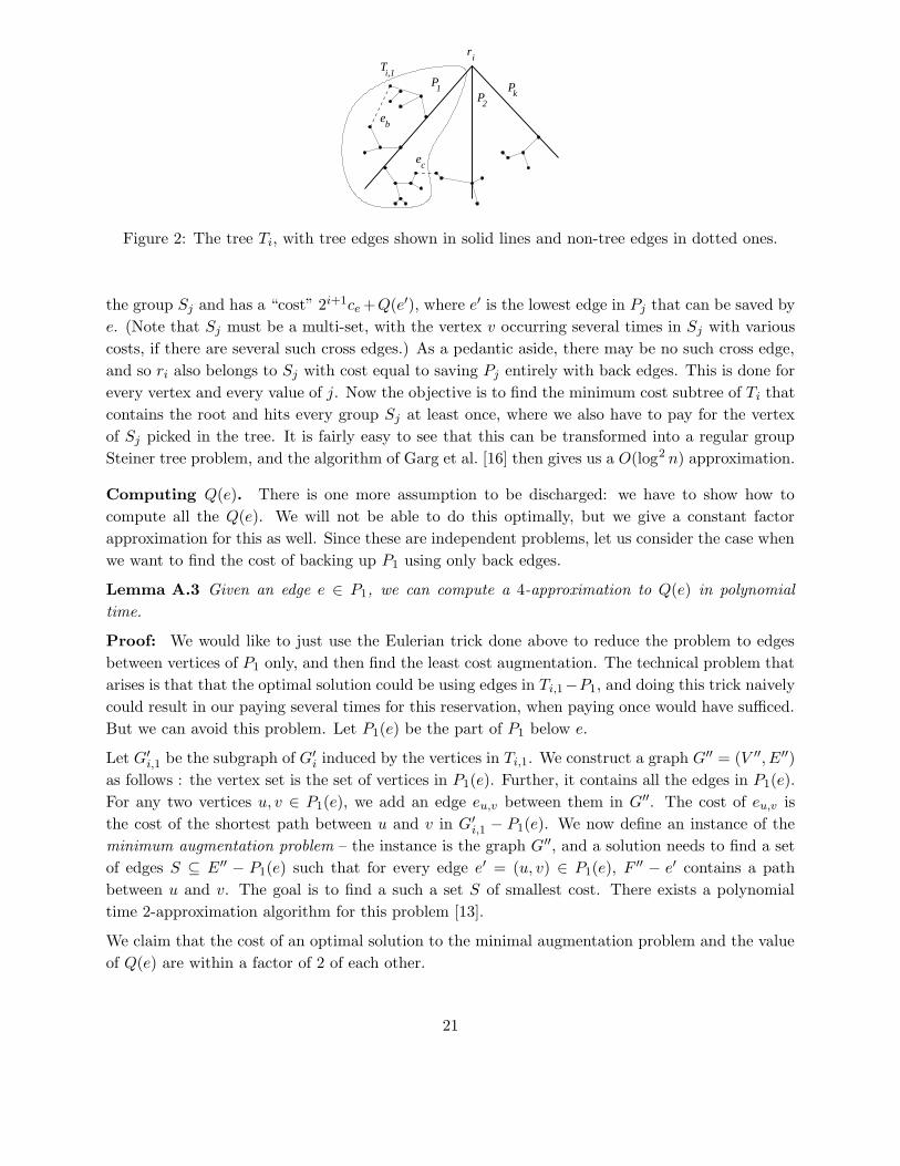
Finding the backup cost in G′i. We now have a simpler problem: a graph G′i, with a spanning

tree Ti in which we need to find a tree backup for the edges of Ei, which form a spider. Let ri be

the root of Ti, and let Pj ’s be the paths of the spider. Also let Ti,j be the subtree of Ti hanging off

Pj . (See Figure 2 for a picture.) Call a non-tree edge a back edge if both its end points belong to

the same tree Ti,j , and a cross edge otherwise. For example, the edge eb is a back edge, and ec a

cross edge in the figure. Now each edge e of Ei has a savior edge sav(e) which is used to connect

the two components formed if e fails. A crucial fact is that if a cross edge from Ti,j to Ti,j′ is a

savior for some edge e in Pj , then it is a savior for all edges on Pj which are above e. Hence, fixing

the lowest edge e in Pj whose savior is a cross edge implies that all edges above it are also saved by

that same savior edge, and all edges below it on Pj must be saved by back edges. The cost Q(e) of

saving the rest by back edges depends on the portion of Ti attached to these edges and the back

edges between this portion; note that this is entirely independent of the rest of the problem.

Suppose we know, for each edge e ∈ ∪jPj , the cost Q(e). (We shall discharge this assumption

later.) Then the cost of backing up all the edges in Ei consists of the following: for each Pj , picking

the single cross edge (say going to Ti,j′) which is going to be savior (and reserving 2i+1 capacity on

it), and reserving 2i+1 capacity on the edges in Ti,j′ from the other end of this edge to the root ri.

Of course, we have to add the cost of saving the edges that were not saved by these cross edges to

the solution.

We now claim that this can be modeled as a minor variant of the group Steiner tree problem with

vertex costs. Each vertex v ∈ Ti which is the endpoint of some cross edge e from Ti,j is belongs to

20

1k

Ti,1

PP

P2

eb

c

ri

e

Figure 2: The tree Ti, with tree edges shown in solid lines and non-tree edges in dotted ones.

the group Sj and has a “cost” 2i+1ce+Q(e′), where e′ is the lowest edge in Pj that can be saved by

e. (Note that Sj must be a multi-set, with the vertex v occurring several times in Sj with various

costs, if there are several such cross edges.) As a pedantic aside, there may be no such cross edge,

and so ri also belongs to Sj with cost equal to saving Pj entirely with back edges. This is done for

every vertex and every value of j. Now the objective is to find the minimum cost subtree of Ti that

contains the root and hits every group Sj at least once, where we also have to pay for the vertex

of Sj picked in the tree. It is fairly easy to see that this can be transformed into a regular group

Steiner tree problem, and the algorithm of Garg et al. [16] then gives us a O(log2 n) approximation.

Computing Q(e). There is one more assumption to be discharged: we have to show how to

compute all the Q(e). We will not be able to do this optimally, but we give a constant factor

approximation for this as well. Since these are independent problems, let us consider the case when

we want to find the cost of backing up P1 using only back edges.

Lemma A.3 Given an edge e ∈ P1, we can compute a 4-approximation to Q(e) in polynomial

time.

Proof: We would like to just use the Eulerian trick done above to reduce the problem to edges

between vertices of P1 only, and then find the least cost augmentation. The technical problem that

arises is that that the optimal solution could be using edges in Ti,1−P1, and doing this trick naively

could result in our paying several times for this reservation, when paying once would have sufficed.

But we can avoid this problem. Let P1(e) be the part of P1 below e.

Let G′i,1 be the subgraph of G′i induced by the vertices in Ti,1. We construct a graph G′′ = (V ′′, E′′)

as follows : the vertex set is the set of vertices in P1(e). Further, it contains all the edges in P1(e).

For any two vertices u, v ∈ P1(e), we add an edge eu,v between them in G′′. The cost of eu,v is

the cost of the shortest path between u and v in G′i,1 − P1(e). We now define an instance of the

minimum augmentation problem – the instance is the graph G′′, and a solution needs to find a set

of edges S ⊆ E ′′ − P1(e) such that for every edge e′ = (u, v) ∈ P1(e), F′′ − e′ contains a path

between u and v. The goal is to find a such a set S of smallest cost. There exists a polynomial

time 2-approximation algorithm for this problem [13].

We claim that the cost of an optimal solution to the minimal augmentation problem and the value

of Q(e) are within a factor of 2 of each other.

21

Suppose we are given a set of edges S ′ such that the S ′ protects the edges in P1(e) in the graph

G′i,1. Clearly, S′ is acyclic. So by taking an Eulerian tour of S ′, we can transform it into a solution

to the above instance of the minimum augmentation problem by doubling its cost.

Let us prove the converse now. Suppose we are given a solution to the minimum augmentation

problem in G′′. Let the set of edges protecting P1(e) be S. Note that no vertex of P1(e) can be

incident with three edges of S – indeed, this would imply that one of these edges is redundant. So,

assuming this is the case, we can map it back to a solution for protecting P1(e) in the graph G′i,1whose cost is at least half the cost of S. This proves the lemma. 2

Thus we have shown the following theorem.

Theorem A.4 Given a polynomial time α-approximation algorithm for the group Steiner tree prob-

lem, there exists a polynomial time algorithm for the backup problem for tree networks that produces

a solution of cost O(α)∑

e ce(up(e) + ub(e)) where ub is a minimum cost feasible backup solution

to the given primary network up.

B Linear Programming Formulations for SSSPR

We provide two linear programming relaxations of SSSPR. The first formulation is based on cuts

and the second formulation is based on flows. We show that the second formulation dominates the

first one on all instances.

A cut in a graph G is a partition of V into two disjoint sets V1 and V2. The edges of the cut are

those edges that have precisely one endpoint in both V1 and V2. Let T be a subgraph of G which

is a tree. A cut (V1, V2) of G is a canonical cut of G with respect to T if there exists an edge e ∈ T ,

decomposing T into T1 and T2, such that T1 ⊆ V1 and T2 ⊆ V2.

Let p be a primary path from the source s to the destination t. It follows from Suurballe’s [31]

procedure that a set of edges q is a backup to a path p if it covers all the canonical cuts of p. This

leads us to the following linear programming formulation which is based on covering cuts. For an

edge e, let x(e) denote the primary indicator variable and let y(e) denote the backup indicator

variable.

min∑

e∈E c1(e) · x(e) + c2(e) · y(e) (Cut-LP)

s.t.∑

e∈C(x(e) + y(e)) ≥ 2 for all s, t-cuts C∑

e∈C x(e) ≥ 1 for all s, t-cuts C

x(e) + y(e) ≤ 1 for all e ∈ E

x(e), y(e) ≥ 0 for all e ∈ E

It is not hard to see that the value of an optimal (fractional) solution to Cut-LP is a lower bound on

the value of an optimal integral solution to SSSPR. We now present a second linear programming

formulation of SSSPR which is based on flows. Our formulation relies on the following lemma.

Lemma B.1 Let p be a primary path from s to t and let q be a set of backup edges. Replace each

edge from p and q by two parallel anti-symmetric unit capacity arcs. Then, two units of flow can

22

be sent from s to t.

Proof: Let path p be s = v1, . . . , vk = t. We send the first unit of flow from s to t through p. For

the second unit of flow we proceed as follows. There has to be a backup edge (s, vi), 1 ≤ i ≤ k.

Let a1 be the arc (s, vi) that maximizes i. There has to be a backup edge (vj , vi′ where 1 ≤ j ≤ i

and i < i′ ≤ k. Let a2 be the arc (vj , vi′) that maximizes i′. We continue this way until we reach

the sink, i.e., the sink is the tail of arc a`. The second unit of flow is sent first on arc a1, then it

goes back in p until it reaches the head of arc a2, then it is sent on arc a2, then it goes back in p

until it reaches the head of arc a3, and so on till it reaches the sink t. 2

This leads us to the following bidirected flow relaxation. We replace each edge by two parallel

anti-symmetric unit capacity arcs. Denote by D = (V,A) the directed graph obtained. The goal

is to send two units of flow in D from s to t, one from each commodity, while minimizing the

cost. Denote the two commodities by blue and red, corresponding to primary and backup edges,

respectively. The cost of the blue commodity on an arc a (obtained from edge e) is equal to c1(e).

The cost of the red commodity on an arc a (obtained from edge e) is defined as follows. Suppose

there is blue flow on arc a− of value f . Then, red flow on a up to value of f is free. Beyond f , the

cost of the red flow is c2(e).

min∑

e∈E c1(e) · f1(e) + c2(e) · f2(e) (Flow-LP)

s.t. x supports a unit flow (f1) between s and t

y supports a unit flow (f2) between s and t

f1(e) ≥ max(f1(a), f1(a−)) for all e = (a, a−)

f2(e) ≥ max((f2(a)− f1(a−)), 0) + max((f2(a

−)− f1(a)), 0)

for all e = (a, a−)

x(a) + y(a) ≤ 1 for all a ∈ A

x(a), y(a) ≥ 0 for all a ∈ A

Given a solution to the SSSPR problem, Lemma B.1 tells us how to obtain a two-commodity flow

solution from it. We claim that the cost of the two-commodity flow solution is equal to the cost of

the solution to the SSSPR problem. Notice that the blue flow costs the same as the blue edges in

the SSSPR solution. The cost of the red flow is zero on arcs which are obtained from blue edges.

On other edges, the cost of the red flow and the cost of the SSSPR solution are the same. Therefore,

the value of an optimal (fractional) solution to the Flow-LP is a lower bound on the value of an

optimal integral solution. We now prove that Flow-LP dominates Cut-LP.

Theorem B.2 For any instance of the SSSPR problem, the cost of the optimal solution produced

by Flow-LP is at least as high as the cost of the optimal solution produced by Cut-LP.

Proof: We show that given a feasible solution to Flow-LP, we can generate a feasible solution to

Cut-LP without increasing the cost. Consider edge e ∈ E which is replaced by two anti parallel arcs

a and a− in Flow-LP. Without loss of generality, we can assume that at most one of f1(a), f1(a−)

is non-zero and at most one of f2(a), f2(a−) is non-zero. Define x(e) = f1(e) (or x(e) = f1(a) +

f1(a−)) and y(e) = min(f2(e), 1− f1(e)). We show that x(e), y(e)e∈E defines a feasible solution

23

for Cut-LP. Let the x-capacity (y-capacity) of a cut be the sum of the variables x(e) (y(e)) taken

over the edges e belonging to the cut. Clearly, the x-capacity of all s, t-cuts is at least one, since

flow f1 in D sends one unit of flow from s to t. It remains to show that the x-capacity together

with the y-capacity of all s, t-cuts is at least two.

Consider a particular s, t-cut C. Decompose flow function f1 in D into flow paths, each of flow

value ε. Let n(k) denote the number of flow paths in the decomposition that use precisely 2k + 1

edges from C. Clearly,∑∞

k=0 n(k) · ε = 1, and so the contribution of flow f1 in D to the x-capacity

of C is

∞∑

k=0

(2k + 1) · n(k) · ε = 2

∞∑

k=0

k · n(k) · ε+∞∑

k=0

n(k) · ε

= 2∞∑

k=0

k · n(k) · ε+ 1.

Suppose∑∞

k=0 k · n(k) · ε < 1/2, otherwise we are done. The red flow in D, f2, can send for “free”

flow of value at most∑∞

k=0 k · n(k) · ε using arcs belonging to cut C. (For each arc a carrying blue

flow of value ε, red flow of value ε can be sent on a− for free.) Therefore, the red flow must send flow

of value at least 1−∑∞

k=0 k ·n(k) ·ε using capacity “paid” for by f2. (Note that for this flow we have

y(e) = f2(e) for all edges e.) Hence, the y-capacity of C is at least 1−∑∞

k=0 k ·n(k) ·ε, yielding that

the capacity of cut C (x-capacity and y-capacity) is 1+2∑∞

k=0 k ·n(k) ·ε+1−∑∞

k=0 k ·n(k) ·ε ≥ 2,

thus completing the proof. 2

0 , 0 0 , 0

0 , 0C , 0

C , 0

C , 0

0 , 0

1 , 1

C , 0 C , 0

0 , 0

0 , 0

0 , 0

ts

1 , 1

0 , 0

C , 0

Figure 3: The gap between optimal fractional and integral solutions is 2.

Integrality Gap. It is not hard to show that a fractional solution to both formulations can

be rounded to an integral solution while increasing the cost by at most a factor of 2. The proof

is along the lines of the proof for the combinatorial 2-approximation algorithm presented earlier.

Unfortunately, this is the best approximation factor that can be obtained by rounding a fractional

solution to Flow-LP. Consider the instance depicted in Figure 3. The cost of the primary and

24

backup flows on each edge e in the graph is denoted by (c1(e), c2(e)). In the figure C is a constant

that is at least 2. In an optimal fractional solution, the primary flow is equally split between the

two dashed paths from s to t and its cost is 1. The backup flow is also equally split between the

two solid paths and its cost is 0. The total fractional cost is thus 1. Any integral solution has

to choose one of the two dashed paths for the primary flow and pay a cost of 1, and then choose

a solid path which is disjoint from the chosen primary path, and pay a cost of 1. Thus, the gap

between optimal fractional and integral solutions is 2.

25