building balance point level 1: introduction to...
TRANSCRIPT
V I T A L S I G N S C U R R I C U L U M M A T E R I A L S P R O J E C T
7 BUILDING BALANCE POINT
INTRODUCTION TO FIRST-ORDERPHYSICAL PRINCIPLES
BALANCING BUILDING ENERGY FLOWS:THE DEFINITION OF THE BUILDING BALANCE POINT TEMPERATURE
The building balance point temperature is a VITAL SIGN indicator of the relationshipbetween the various thermal forces at play within a building; the heat generated bybuilding occupancy, the heat of the sun entering the building, and the transfer ofenergy across the building enclosure due to the difference in temperature betweenbuilding and environment. As a measure of the dynamic interplay of several variables,the building balance point temperature is a powerful conceptual tool used to evaluatethe energy flows between a given building and its surroundings. The building balancepoint can be estimated as a design variable, a function of building design and programvariables. However, it can not be measured directly in the field. All building energyflows must be measured or estimated in the field to estimate the building balancepoint temperature. This section introduces the definition of the balance building pointtemperature, its relationship to building energy flows, and a method of estimatingbuilding energy flows from field observation.
Energy flow out of or into a building is driven by the difference between the building temperature and theoutdoor ambient temperature. The rate of heat flow across the building enclosure is also proportional to thethermal quality of the building enclosure. Occupancy results in building heat gains due to both occupantmetabolism and electric consumption in lights and equipment. Solar energy also adds heat to the building,primarily via glazing transmittance, but also by conduction through the building enclosure when solarenergy is absorbed on the enclosure surface. The balance point temperature is a measure of the conditionsrequired to balance heat entering the building with heat leaving the building in the absence of mechanicalheating or cooling. It is defined as the ambient (or outdoor) air temperature which causes building heattransfer across the enclosure to balance building heat gains at the desired interior temperature (assumed tobe the thermostat setting). This definition of the builfing balance point, T_balance, is given mathemati-cally as:
T balance T thermostat
Q Q
UIHG SOL
bldg
_ _ ˆ= −+
[1]
T_thermostat is the building thermostat setting. QIHG
is the building internal heat generation rate due tooccupancy and given per unit floor area. QSOL is the rate of solar heat gain to the building given per unitfloor area. Ûbldg is the rate of heat transfer across the building enclosure per degree temperature differ-ence, also given per unit floor area. Thus the balance point temperature is defined as the buildingthermostat temperature minus the ratio of total building heat gains divided by the rate of heat transferacross the building enclosure. The elements of the balance point are not constant: Q
IHG changes with the
occupancy schedule and QSOL changes with time of day and time of year. Even Ûbldg can vary due tovariation of the building fresh air ventilation rate.
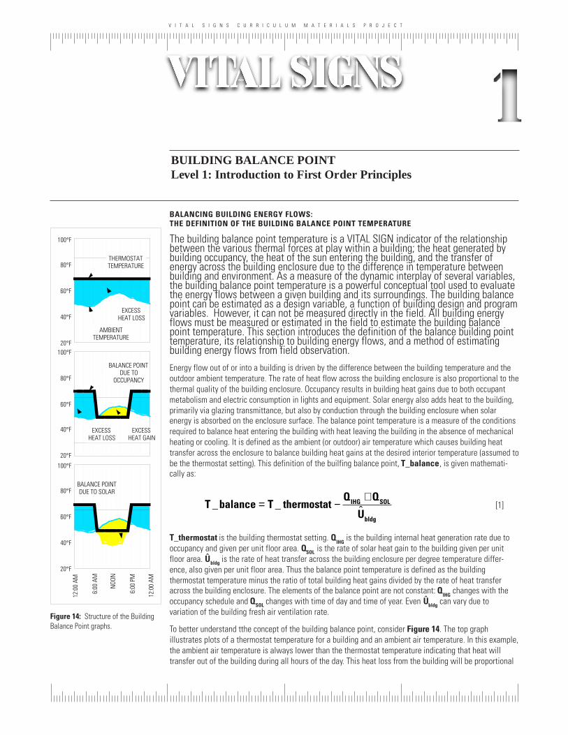
To better understand tthe concept of the building balance point, consider Figure 14. The top graphillustrates plots of a thermostat temperature for a building and an ambient air temperature. In this example,the ambient air temperature is always lower than the thermostat temperature indicating that heat willtransfer out of the building during all hours of the day. This heat loss from the building will be proportional
BUILDING BALANCE POINTLevel 1: Introduction to First Order Principles
Figure 14: Structure of the BuildingBalance Point graphs.
12:0
0 AM
6:00
AM
NOO
N
6:00
PM
12:0
0 AM
20°F
40°F
60°F
80°F
100°F
BALANCE POINT DUE TO SOLAR
20°F
40°F
60°F
80°F
100°F
THERMOSTATTEMPERATURE
AMBIENTTEMPERATURE
EXCESS HEAT LOSS
20°F
40°F
60°F
80°F
100°F
BALANCE POINT DUE TO
OCCUPANCY
EXCESS HEAT LOSS
EXCESS HEAT GAIN
V I T A L S I G N S C U R R I C U L U M M A T E R I A L S P R O J E C T
INTRODUCTION TO FIRST-ORDERPHYSICAL PRINCIPLES
BUILDING BALANCE POINT8
to the temperature difference between the building (or thermostat) temperature and the ambient airtemperature. The thickness of the shaded area is equivelent to the temperature drop across the enclosure.The actual rate of heat transfer across the building enclosure during an hour per unit floor area is equal tothe product of the temperature drop for that hour and the building enclosure heat transfer rate, Ûbldg. Theenclosure heat transfer rate includes heat transfer rates through the roof, walls, glazings and ground, andvia ventilation. It is described in detail later.
The effect of heat gains due to occupancy, QIHG
, is illustrated in the middle graph. When a building isoccupied, heat is added to the building as a result of occupant metabolism and electric energy consump-tion. Many commercial and institutional buildings are occupied during the day, but not at night. When abuilding is unoccupied, its balance point temperature due to internal gains is usually equal to the thermo-stat temperature. The balance point temperature illustrated in the middle plot is equal to the thermostattemperature at night representing an unoccupied building. During the day the balance point temperature isroughly 20°F less than the thermostat temperature. This means that the ratio of QIHG to Ûbldg is equal toroughly 20°F. Note that the balance point temperature has dropped below the ambient air temperatureduring the day, indicating that the internal heat gains will exceed the enclosure heat transfer and thebuilding will experience net heat gains.
Finally, the lower graph illustrates the additional effect of solar heat gains. Solar gains enter primarilythrough the glazing. They will typicall be lower at sunrise and sunset and peak at noon. In this example, theratio of Q
SOL at noon to Û
bldg is roughly 12°F. The total area of net heat gain during the day (the light shaded
area in the lower figure where the balance point is lower than the ambient temperature) is nearly the sameas the total area of net heat loss at night (the darker shaded area where the balance point temperature ishigher than the ambient air temperature). It is the relative magnitudes of areas of net heat gain and netheat loss that permit evaluation of building energy flows using the balance point temperature. The finalgraph in Figure 14 illustrates an area of net heat gain that is slightly smaller than the area of net heat lossat night. Remember, the areas actually represent temperature differences over time, not heat flow. But, dueto the definition of the balance point, the net heat gain (or loss) for the day is given as a product of theshaded area and the enclosure heat transfer rate, Ûbldg.
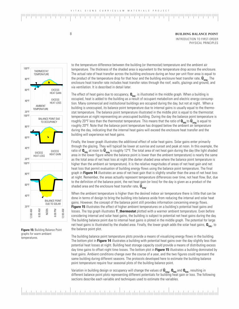
When the ambient temperature is higher than the desired indoor air temperature there is little that can bedone in terms of design to bring the building into balance aside from reducing the internal and solar heatgains. However, the concept of the balance point still provides information concerning energy flows.Figure 15 illustrates the effect of higher ambient temperatures on a building's potential heat gains andlosses. The top graph illustrates T_thermostat plotted with a warmer ambient temperature. Even beforeconsidering internal and solar heat gains, the building is subject to potential net heat gains during the day.The building balance point due to internal heat gains is ploted in the middle graph. The potential for largenet heat gains is illustrated by the shaded area. Finally, the lower graph adds the solar heat gains, QSOL, tothe balance point plot.
The building balance point temperature plots provide a means of visualizing energy flows in the building.The bottom plot in Figure 14 illustrates a building with potential heat gains over the day slightly less thanpotential heat losses at night. Building heat storage capacity could provide a means of distributing excessday time gains to offset night time losses. The bottom plot in Figure 15 illustrates a building dominated byheat gains. Ambient conditions change over the course of a year, and the two figures could represent thesame building during different seasons. The protocols developed here to estimate the building balancepoint temperature require four seasonal plots of the building balance point.
Variation in building design or occupancy will change the values of Ûbldg, QIHG and QSOL, resulting indifferent balance point plots representing different potentials for building heat gain or loss. The followingsections describe each variable and techniques used to estimate the variables.
20°F
40°F
60°F
80°F
100°FBALANCE POINT DUE
TO OCCUPANCY
EXCESS HEAT LOSS
EXCESS HEAT GAIN
20°F
40°F
60°F
80°F
100°FTHERMOSTATTEMPERATURE
AMBIENTTEMPERATURE
EXCESS HEAT LOSS
EXCESS HEAT GAIN
12:0
0 AM
6:00
AM
NOO
N
6:00
PM
12:0
0 AM
20°F
40°F
60°F
80°F
100°F
BALANCE POINT DUE TO SOLAR
Figure 15: Building Balance Pointgraphs for warm ambienttemperatures.
V I T A L S I G N S C U R R I C U L U M M A T E R I A L S P R O J E C T
9 BUILDING BALANCE POINT
INTRODUCTION TO FIRST-ORDERPHYSICAL PRINCIPLES
BUILDING HEAT TRANSFER RATE
While internal heat gains and solar heat gains represent the primary paths for heat entry into buildings,heat transfer across the enclosure represents the primary potential for building heat loss. Heat flowsbetween the building and surrounding environment by two major paths: conduction across the buildingenclosure and bulk air exchange via ventilation or infiltration. The rate of heat flow via either path isproportional to the temperature difference between building and environment. When the environment ishotter than the building, heat flows into the building and the only sources of heat loss are heat flow to theground and mechanical air-conditioning. While accurate computation of the building heat transfer rate canbe complicated, the goal of a balance point evaluation is to provide a reasonable estimate with minimaleffort.
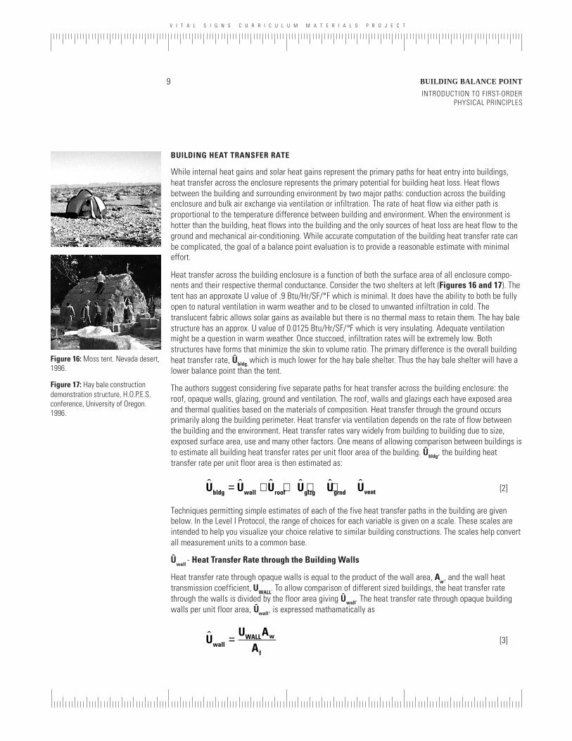
Heat transfer across the building enclosure is a function of both the surface area of all enclosure compo-nents and their respective thermal conductance. Consider the two shelters at left (Figures 16 and 17). Thetent has an approxate U value of .9 Btu/Hr/SF/°F which is minimal. It does have the ability to both be fullyopen to natural ventilation in warm weather and to be closed to unwanted infiltration in cold. Thetranslucent fabric allows solar gains as available but there is no thermal mass to retain them. The hay balestructure has an approx. U value of 0.0125 Btu/Hr/SF/°F which is very insulating. Adequate ventilationmight be a question in warm weather. Once stuccoed, infiltration rates will be extremely low. Bothstructures have forms that minimize the skin to volume ratio. The primary difference is the overall buildingheat transfer rate, Ûbldg, which is much lower for the hay bale shelter. Thus the hay bale shelter will have alower balance point than the tent.
The authors suggest considering five separate paths for heat transfer across the building enclosure: theroof, opaque walls, glazing, ground and ventilation. The roof, walls and glazings each have exposed areaand thermal qualities based on the materials of composition. Heat transfer through the ground occursprimarily along the building perimeter. Heat transfer via ventilation depends on the rate of flow betweenthe building and the environment. Heat transfer rates vary widely from building to building due to size,exposed surface area, use and many other factors. One means of allowing comparison between buildings isto estimate all building heat transfer rates per unit floor area of the building. Ûbldg, the building heattransfer rate per unit floor area is then estimated as:
ˆ ˆ ˆ ˆ ˆ ˆU U U U U Ubldg wall roof glzg grnd vent= + + + + [2]
Techniques permitting simple estimates of each of the five heat transfer paths in the building are givenbelow. In the Level I Protocol, the range of choices for each variable is given on a scale. These scales areintended to help you visualize your choice relative to similar building constructions. The scales help convertall measurement units to a common base.
Ûwall
- Heat Transfer Rate through the Building Walls
Heat transfer rate through opaque walls is equal to the product of the wall area, Aw
, and the wall heattransmission coefficient, U
WALL. To allow comparison of different sized buildings, the heat transfer rate
through the walls is divided by the floor area giving Ûwall. The heat transfer rate through opaque buildingwalls per unit floor area, Ûwall, is expressed mathamatically as
U
U AAwall
WALL w
f
= [3]
Figure 16: Moss tent. Nevada desert,1996.
Figure 17: Hay bale constructiondemonstration structure, H.O.P.E.S.conference, University of Oregon.1996.
V I T A L S I G N S C U R R I C U L U M M A T E R I A L S P R O J E C T
INTRODUCTION TO FIRST-ORDERPHYSICAL PRINCIPLES
BUILDING BALANCE POINT10
The wall area, Aw, and the floor area, Af, can be estimated from field observation or from scale drawings.The wall heat transmission coefficient, UWALL, is estimated based on visual observation in the field or fromconstruction details. While estimation of Aw or Af may be time consuming, the process is straight forward.Two complications can arise when estimating Ûwall. First, the actual wall construction is unknown andU
WALL is difficult estimate. Second, the wall may have more than one type of construction, with a separate
heat transmission coefficient for each construction. Each of these difficulties are considered below.
In practice, UWALL
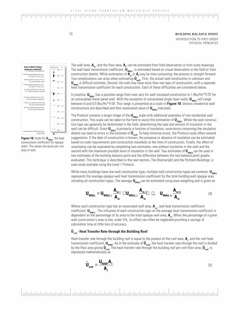
has a possible range from near zero for well insulated construction to 1 Btu/Hr/°F/SF foran uninsulated metal panel wall. With the exception of uninsulated single layer walls, UWALL will rangebetween 0 and 0.5 Btu/Hr/°F/SF. This range is presented as a scale in Figure 18. Various residential wallconstructions are described and their associated value of UWALL indicated.
The Protocol contains a larger image of the UWALL scale with additional examples of non-residential wallconstruction. This scale can be taken to the field to assist the estimation of UWALL. While the wall construc-tion type can generally be determined in the field, determining the type and amount of insulation in thewall can be difficult. Since U
WALL is primarily a function of insulation, uncertainty concerning the insulation
details can lead to errors in the estimate of Ûwall. To help minimize errors, the Protocol scale offers severalsuggestions. If the date of construction is known, the presence or absence of insulation can be estimatedbased on code requirements and construction standards at the time of construction. Finally, the effect ofuncertainty can be evaluated by completing two estimates, one without insulation in the wall and thesecond with the maximum possible level of insulation in the wall. Two estimates of U
WALL can be used in
two estimates of the building balance point and the difference between the two balance point graphsevaluated. This technique is described in the next section, The Wainwright and the Portland Buildings: acase study example using the Level 1 Protocol.
While many buildings have one wall construction type, multiple wall construction types are common. UWALL
represents the average opaque wall heat transmission coefficient for the total building wall opaque areaincluding all construction types. The average UWALL can be estimated using area weighting and is given as
U U
AA
UAA
UAAWALL WALL
w
wWALL
w
wWALL n
w n
w
= + + +,,
,,
,,...1
12
2 [4]
Where each construction type has an associated wall area, Aw,i
, and heat transmission coefficientcoefficient, U
WALL,i. The influence of each construction type on the average heat transmission coefficient is
dependant on the percentage of its area to the total opaque wall area, Aw. When the percentage of a givenwall construction's area is low, under 5%, its effect can often be neglected providing a savings ofcalculation time at little loss of accuracy.
Ûroof - Heat Transfer Rate through the Building Roof
Heat transfer rate through the building roof is equal to the product of the roof area, Ar, and the roof heattransmission coefficient, UROOF. As in the estimate of Ûwall, the heat transfer rate through the roof is dividedby the floor area giving Ûroof. The heat transfer rate through the building roof per unit floor area, Ûroof, isexpressed mathamatically as
U
U AAroof
ROOF r
f
= [5]
Scale of Wall U Values(primarily residential) 0.00
0.20
0.15
0.30
0.25
0.40
0.35
0.50
0.45
0.10
0.05
Btu/Hr/SF/°F∞
5
6.7
3.3
4
2.5
2.8
2
2.2
10
20
R
24” straw bale, stucco both sides
thermally broken stud wall, 6” insul. (typ. superinsulated const.)
wd. siding, sheathing, 2x4 wd. stud, 3.5” insulation. (typical residential)
4” brick, wd. sheathing, 2x4 wd. stud, wd. lath, plaster (traditional)
wd. siding, sheathing, 2x4 wd. stud, g.w.b. (uninsulated residential)
wd. siding, sheathing, 2x4 wd. stud, wd. lath, plaster (traditional)
uninsulated steel siding, metal frame bldg. (U=.98)
1” EIFS (expanded polystyrene) g.w.b., 2x4 stud, 3.5” insul., g.w.b.
2” EIFS (expanded polystyrene) g.w.b., 2x4 stud, 3.5” insul., g.w.b.
Figure 18: Scale for UWALL, the heattransmission coefficient for opaquewalls. The values are given per unitarea of wall.
V I T A L S I G N S C U R R I C U L U M M A T E R I A L S P R O J E C T
11 BUILDING BALANCE POINT
INTRODUCTION TO FIRST-ORDERPHYSICAL PRINCIPLES
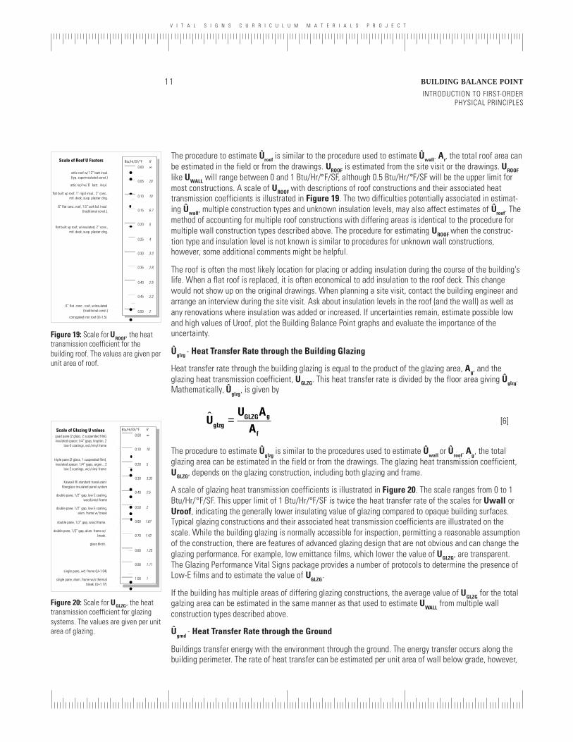
The procedure to estimate Ûroof is similar to the procedure used to estimate Ûwall. Ar, the total roof area canbe estimated in the field or from the drawings. UROOF is estimated from the site visit or the drawings. UROOF
like UWALL will range between 0 and 1 Btu/Hr/°F/SF, although 0.5 Btu/Hr/°F/SF will be the upper limit formost constructions. A scale of UROOF with descriptions of roof constructions and their associated heattransmission coefficients is illustrated in Figure 19. The two difficulties potentially associated in estimat-ing Ûwall, multiple construction types and unknown insulation levels, may also affect estimates of Ûroof. Themethod of accounting for multiple roof constructions with differing areas is identical to the procedure formultiple wall construction types described above. The procedure for estimating UROOF when the construc-tion type and insulation level is not known is similar to procedures for unknown wall constructions,however, some additional comments might be helpful.
The roof is often the most likely location for placing or adding insulation during the course of the building'slife. When a flat roof is replaced, it is often economical to add insulation to the roof deck. This changewould not show up on the original drawings. When planning a site visit, contact the building engineer andarrange an interview during the site visit. Ask about insulation levels in the roof (and the wall) as well asany renovations where insulation was added or increased. If uncertainties remain, estimate possible lowand high values of Uroof, plot the Building Balance Point graphs and evaluate the importance of theuncertainty.
Ûglzg - Heat Transfer Rate through the Building Glazing
Heat transfer rate through the building glazing is equal to the product of the glazing area, Ag, and theglazing heat transmission coefficient, UGLZG. This heat transfer rate is divided by the floor area giving Ûglzg.Mathematically, Û
glzg, is given by
U
U AAglzg
GLZG g
f
= [6]
The procedure to estimate Ûglzg
is similar to the procedures used to estimate Ûwall
or Ûroof
. Ag, the total
glazing area can be estimated in the field or from the drawings. The glazing heat transmission coefficient,UGLZG, depends on the glazing construction, including both glazing and frame.
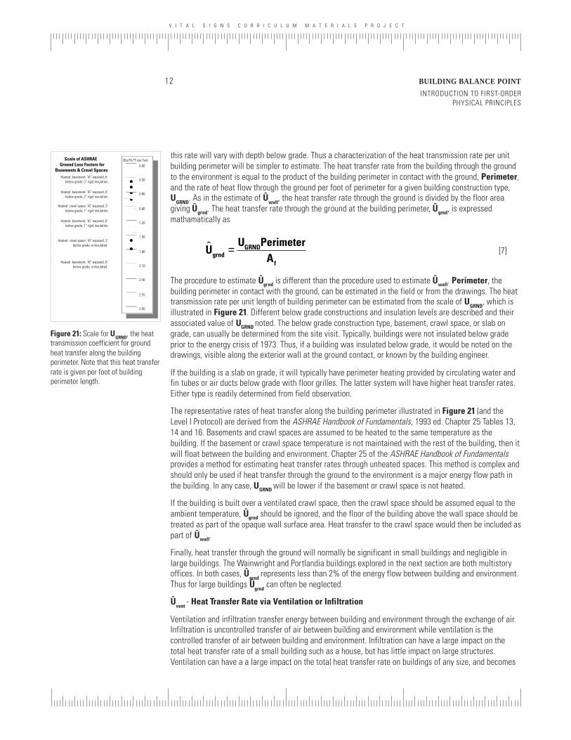
A scale of glazing heat transmission coefficients is illustrated in Figure 20. The scale ranges from 0 to 1Btu/Hr/°F/SF. This upper limit of 1 Btu/Hr/°F/SF is twice the heat transfer rate of the scales for Uwall orUroof, indicating the generally lower insulating value of glazing compared to opaque building surfaces.Typical glazing constructions and their associated heat transmission coefficients are illustrated on thescale. While the building glazing is normally accessible for inspection, permitting a reasonable assumptionof the construction, there are features of advanced glazing design that are not obvious and can change theglazing performance. For example, low emittance films, which lower the value of UGLZG, are transparent.The Glazing Performance Vital Signs package provides a number of protocols to determine the presence ofLow-E films and to estimate the value of U
GLZG.
If the building has multiple areas of differing glazing constructions, the average value of UGLZG for the totalgalzing area can be estimated in the same manner as that used to estimate U
WALL from multiple wall
construction types described above.
Ûgrnd
- Heat Transfer Rate through the Ground
Buildings transfer energy with the environment through the ground. The energy transfer occurs along thebuilding perimeter. The rate of heat transfer can be estimated per unit area of wall below grade, however,
Scale of Glazing U values0.00
0.40
0.30
0.60
0.50
0.80
0.70
1.00
0.90
0.20
0.10
Btu/Hr/SF/°F∞
2.5
3.33
1.67
2
1.25
1.43
1
1.11
5
10
R
quad pane (2 glass, 2 suspended film), insulated spacer,1/4” gaps, krypton, 2
low-E coatings, wd./vinyl frame
triple pane (2 glass, 1 suspended film), insulated spacer, 1/4” gaps, argon, , 2
low E coatings, wd./vinyl frame
double pane, 1/2” gap, low E coating, wood/vinyl frame
double pane, 1/2” gap, wood frame.
double pane, 1/2” gap, low E coating, alum. frame w/ break
glass block.
single pane, wd. frame (U=1.04)
single pane, alum. frame w/o thermal break. (U=1.17)
double pane, 1/2” gap, alum. frame w/ break.
Kalwall ® standard translucent fiberglass insulated panel system
0.00
0.20
0.15
0.30
0.25
0.40
0.35
0.50
0.45
0.10
0.05
Btu/Hr/SF/°F∞
5
6.7
3.3
4
2.5
2.8
2
2.2
10
20
R Scale of Roof U Factors
attic roof w/ 12” batt insul.(typ. superinsulated const.)
attic roof w/ 6’ batt . insul.
6” flat conc. roof, uninsulated(traditional const.)
flat built up roof, 1” rigid insul., 2” conc., mtl. deck, susp. plaster clng.
6” flat conc. roof, 1.5” cork bd. insul. (traditional const.).
flat built up roof, uninsulated, 2” conc., mtl. deck, susp. plaster clng.
corrugated iron roof (U=1.5)
Figure 19: Scale for UROOF, the heattransmission coefficient for thebuilding roof. The values are given perunit area of roof.
Figure 20: Scale for UGLZG, the heattransmission coefficient for glazingsystems. The values are given per unitarea of glazing.
V I T A L S I G N S C U R R I C U L U M M A T E R I A L S P R O J E C T
INTRODUCTION TO FIRST-ORDERPHYSICAL PRINCIPLES
BUILDING BALANCE POINT12
this rate will vary with depth below grade. Thus a characterization of the heat transmission rate per unitbuilding perimeter will be simpler to estimate. The heat transfer rate from the building through the groundto the environment is equal to the product of the building perimeter in contact with the ground, Perimeter,and the rate of heat flow through the ground per foot of perimeter for a given building construction type,U
GRND. As in the estimate of Û
wall, the heat transfer rate through the ground is divided by the floor area
giving Ûgrnd. The heat transfer rate through the ground at the building perimeter, Ûgrnd, is expressedmathamatically as
U
U PerimeterAgrnd
GRND
f
= [7]
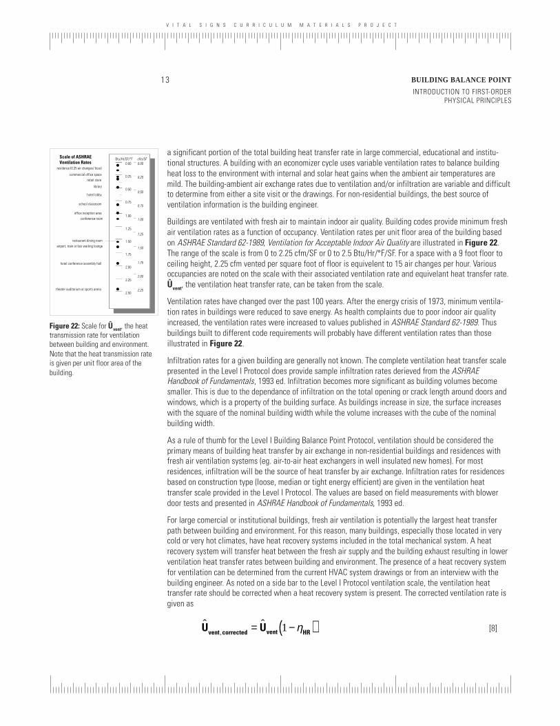
The procedure to estimate Ûgrnd is different than the procedure used to estimate Ûwall. Perimeter, thebuilding perimeter in contact with the ground, can be estimated in the field or from the drawings. The heattransmission rate per unit length of building perimeter can be estimated from the scale of U
GRND, which is
illustrated in Figure 21. Different below grade constructions and insulation levels are described and theirassociated value of UGRND noted. The below grade construction type, basement, crawl space, or slab ongrade, can usually be determined from the site visit. Typically, buildings were not insulated below gradeprior to the energy crisis of 1973. Thus, if a building was insulated below grade, it would be noted on thedrawings, visible along the exterior wall at the ground contact, or known by the building engineer.
If the building is a slab on grade, it will typically have perimeter heating provided by circulating water andfin tubes or air ducts below grade with floor grilles. The latter system will have higher heat transfer rates.Either type is readily determined from field observation.
The representative rates of heat transfer along the building perimeter illustrated in Figure 21 (and theLevel I Protocol) are derived from the ASHRAE Handbook of Fundamentals, 1993 ed. Chapter 25 Tables 13,14 and 16. Basements and crawl spaces are assumed to be heated to the same temperature as thebuilding. If the basement or crawl space temperature is not maintained with the rest of the building, then itwill float between the building and environment. Chapter 25 of the ASHRAE Handbook of Fundamentalsprovides a method for estimating heat transfer rates through unheated spaces. This method is complex andshould only be used if heat transfer through the ground to the environment is a major energy flow path inthe building. In any case, UGRND will be lower if the basement or crawl space is not heated.
If the building is built over a ventilated crawl space, then the crawl space should be assumed equal to theambient temperature, Ûgrnd should be ignored, and the floor of the building above the wall space should betreated as part of the opaque wall surface area. Heat transfer to the crawl space would then be included aspart of Ûwall.
Finally, heat transfer through the ground will normally be significant in small buildings and negligible inlarge buildings. The Wainwright and Portlandia buildings explored in the next section are both multistoryoffices. In both cases, Û
grnd represents less than 2% of the energy flow between building and environment.
Thus for large buildings Ûgrnd
can often be neglected.
Ûvent
- Heat Transfer Rate via Ventilation or Infiltration
Ventilation and infiltration transfer energy between building and environment through the exchange of air.Infiltration is uncontrolled transfer of air between building and environment while ventilation is thecontrolled transfer of air between building and environment. Infiltration can have a large impact on thetotal heat transfer rate of a small building such as a house, but has little impact on large structures.Ventilation can have a a large impact on the total heat transfer rate on buildings of any size, and becomes
Scale of ASHRAE Ground Loss Factors for
Basements & Crawl Spaces0.00
1.20
0.90
1.80
1.50
2.40
2.10
3.00
2.70
0.60
0.30
Btu/Hr/°F per Foot
Heated basement; 16” exposed, 6’ below grade; 3” rigid insulation.
Heated basement; 16” exposed, 6’ below grade; 2” rigid insulation.
Heated basement; 16” exposed, 6’ below grade; 1” rigid insulation.
Heated basement; 16” exposed, 6’ below grade; uninsulated.
Heated crawl space; 16” exposed, 3’ below grade; uninsulated.
Heated crawl space; 16” exposed, 3’ below grade; 1” rigid insulation.
Figure 21: Scale for UGRND, the heattransmission coefficient for groundheat transfer along the buildingperimeter. Note that this heat transferrate is given per foot of buildingperimeter length.
V I T A L S I G N S C U R R I C U L U M M A T E R I A L S P R O J E C T
13 BUILDING BALANCE POINT
INTRODUCTION TO FIRST-ORDERPHYSICAL PRINCIPLES
a significant portion of the total building heat transfer rate in large commercial, educational and institu-tional structures. A building with an economizer cycle uses variable ventilation rates to balance buildingheat loss to the environment with internal and solar heat gains when the ambient air temperatures aremild. The building-ambient air exchange rates due to ventilation and/or infiltration are variable and difficultto determine from either a site visit or the drawings. For non-residential buildings, the best source ofventilation information is the building engineer.
Buildings are ventilated with fresh air to maintain indoor air quality. Building codes provide minimum freshair ventilation rates as a function of occupancy. Ventilation rates per unit floor area of the building basedon ASHRAE Standard 62-1989, Ventilation for Acceptable Indoor Air Quality are illustrated in Figure 22.The range of the scale is from 0 to 2.25 cfm/SF or 0 to 2.5 Btu/Hr/°F/SF. For a space with a 9 foot floor toceiling height, 2.25 cfm vented per square foot of floor is equivelent to 15 air changes per hour. Variousoccupancies are noted on the scale with their associated ventilation rate and equivelant heat transfer rate.Ûvent, the ventilation heat transfer rate, can be taken from the scale.
Ventilation rates have changed over the past 100 years. After the energy crisis of 1973, minimum ventila-tion rates in buildings were reduced to save energy. As health complaints due to poor indoor air qualityincreased, the ventilation rates were increased to values published in ASHRAE Standard 62-1989. Thusbuildings built to different code requirements will probably have different ventilation rates than thoseillustrated in Figure 22.
Infiltration rates for a given building are generally not known. The complete ventilation heat transfer scalepresented in the Level I Protocol does provide sample infiltration rates derieved from the ASHRAEHandbook of Fundamentals, 1993 ed. Infiltration becomes more significant as building volumes becomesmaller. This is due to the dependance of infiltration on the total opening or crack length around doors andwindows, which is a property of the building surface. As buildings increase in size, the surface increaseswith the square of the nominal building width while the volume increases with the cube of the nominalbuilding width.
As a rule of thumb for the Level I Building Balance Point Protocol, ventilation should be considered theprimary means of building heat transfer by air exchange in non-residential buildings and residences withfresh air ventilation systems (eg. air-to-air heat exchangers in well insulated new homes). For mostresidences, infiltration will be the source of heat transfer by air exchange. Infiltration rates for residencesbased on construction type (loose, median or tight energy efficient) are given in the ventilation heattransfer scale provided in the Level I Protocol. The values are based on field measurements with blowerdoor tests and presented in ASHRAE Handbook of Fundamentals, 1993 ed.
For large comercial or institutional buildings, fresh air ventilation is potentially the largest heat transferpath between building and environment. For this reason, many buildings, especially those located in verycold or very hot climates, have heat recovery systems included in the total mechanical system. A heatrecovery system will transfer heat between the fresh air supply and the building exhaust resulting in lowerventilation heat transfer rates between building and environment. The presence of a heat recovery systemfor ventilation can be determined from the current HVAC system drawings or from an interview with thebuilding engineer. As noted on a side bar to the Level I Protocol ventilation scale, the ventilation heattransfer rate should be corrected when a heat recovery system is present. The corrected ventilation rate isgiven as
ˆ ˆ
,U Uvent corrected vent HR= −( )1 η [8]
Scale of ASHRAEVentilation Rates 0.00
1.00
0.75
1.50
1.25
2.00
1.75
2.25
0.50
0.25
Btu/Hr/SF/°F cfm/SF 0.00
1.00
0.75
1.50
1.25
2.00
1.75
2.50
2.25
0.50
0.25
residence (0.35 air changes/ hour)
commercial office space
library
school classroom
hotel lobby
retail store
office reception areaconference room
restaurant dining roomairport, train or bus waiting lounge
hotel conference assembly hall
theater auditorium or sports arena
Figure 22: Scale for Ûvent, the heattransmission rate for ventilationbetween building and environment.Note that the heat transmission rateis given per unit floor area of thebuilding.
V I T A L S I G N S C U R R I C U L U M M A T E R I A L S P R O J E C T
INTRODUCTION TO FIRST-ORDERPHYSICAL PRINCIPLES
BUILDING BALANCE POINT14
Where Ûvent is the ventilation heat transfer rate without heat recovery and ηHR is the heat recovery systemefficiency, typically between 60% and 80%.
The ventilation heat transfer rate is often the least known path of heat transfer in the building with thelargest margin of error in the estimate. To account for this uncertainty, performing two balance pointanalyses with expected minimum and maximum ranges of Ûvent is often the most appropriate means ofevaluating the effects of ventilation. The case study comparison of the Wainwright and Portlandia buildingspresented in the next section illustrates this technique.
BUILDING INTERNAL HEAT GAINS
The two flow paths for building heat gains are internal heat generation due to occupancy, QIHG
, and solarheat gains, Q
SOL. Internal heat gains are considered in this subsection while solar heat gains will be
considered in the following subsection.
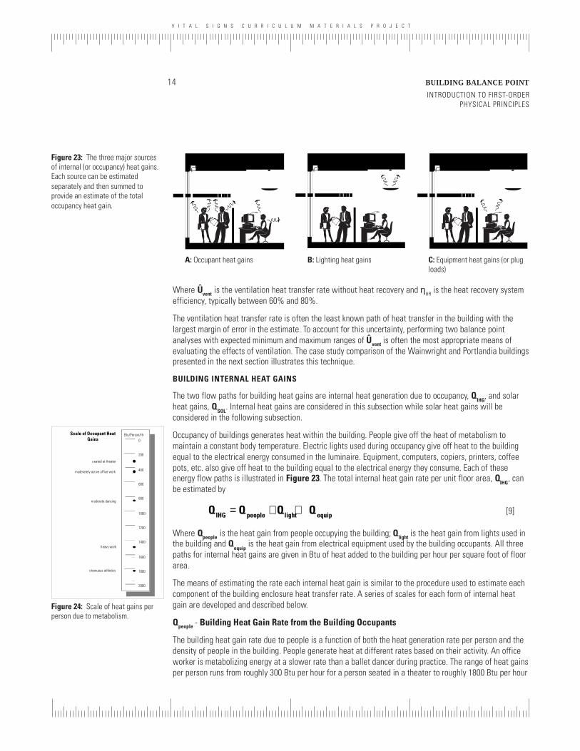
Occupancy of buildings generates heat within the building. People give off the heat of metabolism tomaintain a constant body temperature. Electric lights used during occupancy give off heat to the buildingequal to the electrical energy consumed in the luminaire. Equipment, computers, copiers, printers, coffeepots, etc. also give off heat to the building equal to the electrical energy they consume. Each of theseenergy flow paths is illustrated in Figure 23. The total internal heat gain rate per unit floor area, Q
IHG, can
be estimated by
Q Q Q QIHG people light equip= + + [9]
Where Qpeople is the heat gain from people occupying the building; Qlight is the heat gain from lights used inthe building and Q
equip is the heat gain from electrical equipment used by the building occupants. All three
paths for internal heat gains are given in Btu of heat added to the building per hour per square foot of floorarea.
The means of estimating the rate each internal heat gain is similar to the procedure used to estimate eachcomponent of the building enclosure heat transfer rate. A series of scales for each form of internal heatgain are developed and described below.
Qpeople - Building Heat Gain Rate from the Building Occupants
The building heat gain rate due to people is a function of both the heat generation rate per person and thedensity of people in the building. People generate heat at different rates based on their activity. An officeworker is metabolizing energy at a slower rate than a ballet dancer during practice. The range of heat gainsper person runs from roughly 300 Btu per hour for a person seated in a theater to roughly 1800 Btu per hour
0
800
600
1200
1000
1600
1400
2000
1800
400
200
Btu/Person/HrScale of Occupant Heat Gains
seated at theater
moderately active office work
heavy work
s trenuous athletics
moderate dancing
Figure 23: The three major sourcesof internal (or occupancy) heat gains.Each source can be estimatedseparately and then summed toprovide an estimate of the totaloccupancy heat gain.
A: Occupant heat gains B: Lighting heat gains C: Equipment heat gains (or plugloads)
Figure 24: Scale of heat gains perperson due to metabolism.
V I T A L S I G N S C U R R I C U L U M M A T E R I A L S P R O J E C T
15 BUILDING BALANCE POINT
INTRODUCTION TO FIRST-ORDERPHYSICAL PRINCIPLES
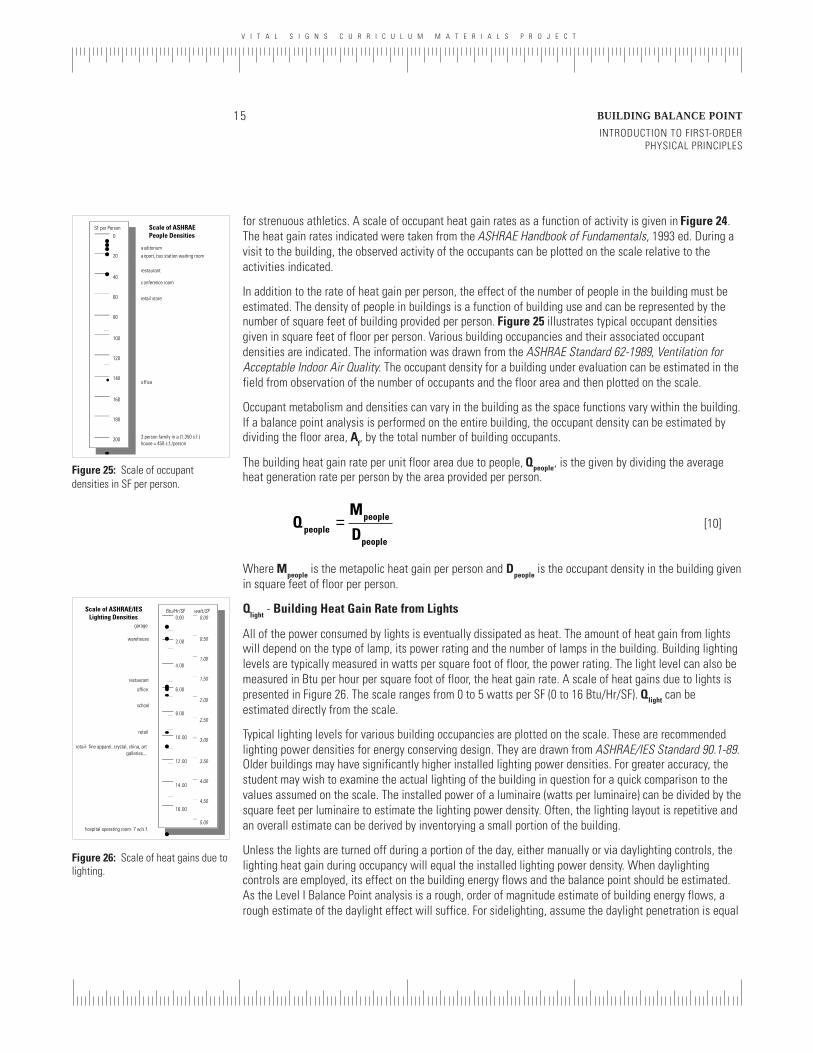
for strenuous athletics. A scale of occupant heat gain rates as a function of activity is given in Figure 24.The heat gain rates indicated were taken from the ASHRAE Handbook of Fundamentals, 1993 ed. During avisit to the building, the observed activity of the occupants can be plotted on the scale relative to theactivities indicated.
In addition to the rate of heat gain per person, the effect of the number of people in the building must beestimated. The density of people in buildings is a function of building use and can be represented by thenumber of square feet of building provided per person. Figure 25 illustrates typical occupant densitiesgiven in square feet of floor per person. Various building occupancies and their associated occupantdensities are indicated. The information was drawn from the ASHRAE Standard 62-1989, Ventilation forAcceptable Indoor Air Quality. The occupant density for a building under evaluation can be estimated in thefield from observation of the number of occupants and the floor area and then plotted on the scale.
Occupant metabolism and densities can vary in the building as the space functions vary within the building.If a balance point analysis is performed on the entire building, the occupant density can be estimated bydividing the floor area, A
f, by the total number of building occupants.
The building heat gain rate per unit floor area due to people, Qpeople, is the given by dividing the averageheat generation rate per person by the area provided per person.
Q people =
Mpeople
Dpeople
[10]
Where Mpeople
is the metapolic heat gain per person and Dpeople
is the occupant density in the building givenin square feet of floor per person.
Qlight
- Building Heat Gain Rate from Lights
All of the power consumed by lights is eventually dissipated as heat. The amount of heat gain from lightswill depend on the type of lamp, its power rating and the number of lamps in the building. Building lightinglevels are typically measured in watts per square foot of floor, the power rating. The light level can also bemeasured in Btu per hour per square foot of floor, the heat gain rate. A scale of heat gains due to lights ispresented in Figure 26. The scale ranges from 0 to 5 watts per SF (0 to 16 Btu/Hr/SF). Qlight can beestimated directly from the scale.
Typical lighting levels for various building occupancies are plotted on the scale. These are recommendedlighting power densities for energy conserving design. They are drawn from ASHRAE/IES Standard 90.1-89.Older buildings may have significantly higher installed lighting power densities. For greater accuracy, thestudent may wish to examine the actual lighting of the building in question for a quick comparison to thevalues assumed on the scale. The installed power of a luminaire (watts per luminaire) can be divided by thesquare feet per luminaire to estimate the lighting power density. Often, the lighting layout is repetitive andan overall estimate can be derived by inventorying a small portion of the building.
Unless the lights are turned off during a portion of the day, either manually or via daylighting controls, thelighting heat gain during occupancy will equal the installed lighting power density. When daylightingcontrols are employed, its effect on the building energy flows and the balance point should be estimated.As the Level I Balance Point analysis is a rough, order of magnitude estimate of building energy flows, arough estimate of the daylight effect will suffice. For sidelighting, assume the daylight penetration is equal
0
80
60
120
100
160
140
200
180
40
20
SF per Person Scale of ASHRAE People Densities
office
retail store
conference room
airport, bus station waiting room
restaurant
auditorium
3 person family in a (1,350 s.f.) house = 450 s.f./person
Figure 25: Scale of occupantdensities in SF per person.
Scale of ASHRAE/IES Lighting Densities 0.00
2.00
1.50
3.00
2.50
4.00
3.50
5.00
4.50
1.00
0.50
Btu/Hr/SF watt/SF0.00
8.00
6.00
12 .00
10 .00
16 .00
14 .00
4.00
2.00
garage
warehouse
office.
retail
school
restaurant
retail- fine apparel, crystal, china, art galleries....
hospital operating room- 7 w/s.f.
Figure 26: Scale of heat gains due tolighting.
V I T A L S I G N S C U R R I C U L U M M A T E R I A L S P R O J E C T
INTRODUCTION TO FIRST-ORDERPHYSICAL PRINCIPLES
BUILDING BALANCE POINT16
Figure 28: Solar heat gains throughthe building glazing.
to twice the head height of the window. For a skylight, assume that daylight illuminates the area under theskylight and a distance into the space equal to the floor to ceiling height of the space. Using these twoassumptions, determine the percentage of the total floor area that is daylit, ƒdaylight. The corrected heat gainfrom lights, Qlight,cor, is then estimated by
Qlight ,cor = Qlight 1 −
ƒdaylight
2
[11]
This method is rough and assumes that all daylit areas require only half the lighting power of non-daylitareas. An evaluation of the effect of daylighting can be developed by
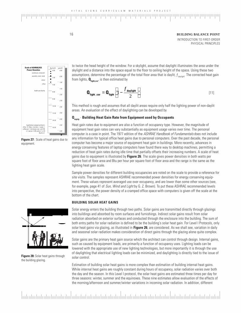
Qequip - Building Heat Gain Rate from Equipment used by Occupants
Heat gain rates due to equipment are also a function of occupancy type. However, the magnitude ofequipment heat gain rates can vary substantially as equipment usage varies over time. The personalcomputer is a case in point. The 1977 edition of the ASHRAE Handbook of Fundamentals does not includeany information for typical office heat gains due to personal computers. Over the past decade, the personalcomputer has become a major source of equipment heat gain in buildings. More recently, advances inenergy conserving features of laptop computers have found there way to desktop machines, permitting areduction of heat gain rates during idle time that partially offsets their increasing numbers. A scale of heatgains due to equipment is illustrated by Figure 26. The scale gives power densities in both watts persquare foot of floor area and Btu per hour per square foot of floor area and the range is the same as thelighting heat gain scale.
Sample power densities for different building occupancies are noted on the scale to provide a reference forsite visits. The samples represent ASHRAE recommended power densities for energy conserving equip-ment. These values represent averaged use over occupancy, and are lower than some other sources (see,for example, page 41 of Sun, Wind and Light by G. Z. Brown). To put these ASHRAE recommended levelsinto perspective, the power density of a cramped office space with computers is given off the scale at thebottom of the chart.
BUILDING SOLAR HEAT GAINS
Solar energy enters the building through two paths. Solar gains are transmitted directly through glazingsinto buildings and absorbed by room surfaces and furnishings. Indirect solar gains result from solarradiation absorbed on exterior surfaces and conducted through the enclosure into the building. The sum ofboth entry paths for solar radiation is defined to be the building's solar heat gain. For Level I Protocols, onlysolar heat gains via glazing, as illustrated in Figure 26, are considered. As we shall see, variation in dailyand seasonal solar radiation makes consideration of direct gains through the glazing alone quite complex.
Solar gains are the primary heat gain source which the architect can control through design. Internal gains,such as caused by equipment loads, are primarily a function of occupancy uses. Lighting loads can belowered with the appropriate use of new lighting technologies, but more importantly it is through the useof daylighting that electrical lighting loads can be minimized, and daylighting is directly tied to the issue ofsolar control.
Estimation of building solar heat gains is more complex than estimation of building internal heat gains.While internal heat gains are roughly constant during hours of occupancy, solar radiation varies over boththe day and the season. In this Level I protocol, the solar heat gains are estimated three times per day forthree seasons: winter, summer and the equinoxes. These nine estimates allow evaluation of the effects ofthe morning/afternoon and summer/winter variations in incoming solar radiation. In addition, different
0.00
2.00
1.50
3.00
2.50
4.00
3.50
5.00
4.50
1.00
0.50
Btu/Hr/SF watt/SF 0.00
8.00
6.00
12 .00
10 .00
16 .00
14 .00
4.00
2.00
Scale of ASHRAE/IESPower Densities
warehouse, restaurant
assembly, retail, motel
office
hypothetical cramped architect’s office- 10 Macs, 2 printers, 1 copier, 1 coffee pot, 1 microwave oven and 100
s.f./ person= 5.86 watts/s.f. or 20 Btu/hr/s.f.
health care facility
school
Figure 27: Scale of heat gains due toequipment.
V I T A L S I G N S C U R R I C U L U M M A T E R I A L S P R O J E C T
17 BUILDING BALANCE POINT
INTRODUCTION TO FIRST-ORDERPHYSICAL PRINCIPLES
building orientations receive different rates of solar energy during the same hour and each major glazingsurface must be accounted for individually. Typically this means examining the solar apertures on fourbuilding orientations and possibly a roof skylight or atrium, though if the building (or room) under investiga-tion doesn't have apertures on all of its elevations, the blank surfaces can be ignored.
Solar radiation levels vary not only with solar geometry, but also with clouds. Furthermore, the amount ofincident solar radiation transmitted by a window will depend on both the glazing's optical characteristicsand the external shading strategy. At this level of study, the goal is to get a rough estimate of the scale ofbuilding solar heat gains relative to other paths of heat flow in the building.
To reduce this complexity to manageable proportions, average solar gains admitted by standard glass areprovided for three times of day for three seasons and five orientations (45 solar gain values for eachclimate). This solar data is provided in tabular for for 14 United States sites in Appendix 4. In addition, theExcel spreadsheet BPgraph.xla contains the 45 solar gain values for 72 cities scattered throughout theworld. A table of the 32 US and 39 global cities included with BPgraph.xla is given in Appendix 4. Adescription of BPgraph.xla is given in Appendix 3.
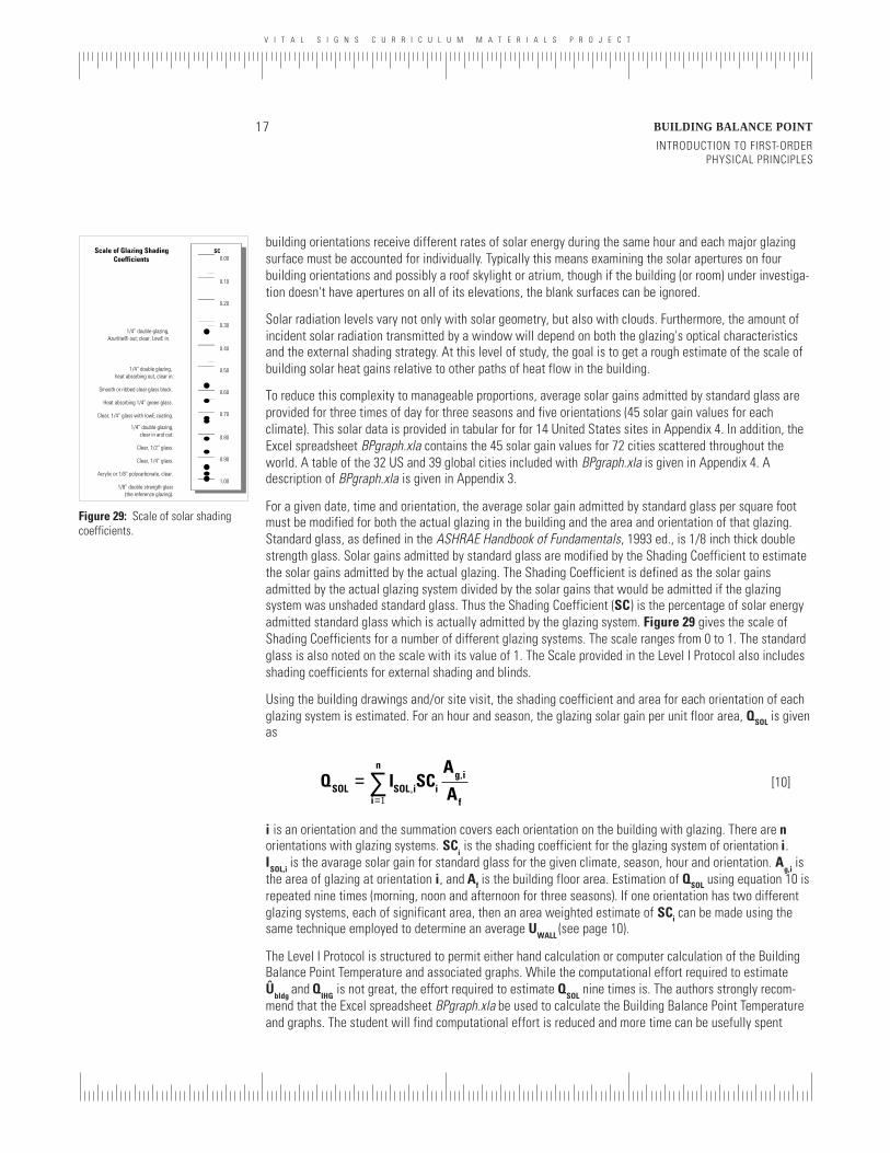
For a given date, time and orientation, the average solar gain admitted by standard glass per square footmust be modified for both the actual glazing in the building and the area and orientation of that glazing.Standard glass, as defined in the ASHRAE Handbook of Fundamentals, 1993 ed., is 1/8 inch thick doublestrength glass. Solar gains admitted by standard glass are modified by the Shading Coefficient to estimatethe solar gains admitted by the actual glazing. The Shading Coefficient is defined as the solar gainsadmitted by the actual glazing system divided by the solar gains that would be admitted if the glazingsystem was unshaded standard glass. Thus the Shading Coefficient (SC) is the percentage of solar energyadmitted standard glass which is actually admitted by the glazing system. Figure 29 gives the scale ofShading Coefficients for a number of different glazing systems. The scale ranges from 0 to 1. The standardglass is also noted on the scale with its value of 1. The Scale provided in the Level I Protocol also includesshading coefficients for external shading and blinds.
Using the building drawings and/or site visit, the shading coefficient and area for each orientation of eachglazing system is estimated. For an hour and season, the glazing solar gain per unit floor area, QSOL is givenas
Q I SC
A
ASOL SOL i ig i
fi
n
==∑ ,
,
1
[10]
i is an orientation and the summation covers each orientation on the building with glazing. There are norientations with glazing systems. SC
i is the shading coefficient for the glazing system of orientation i.
ISOL,i
is the avarage solar gain for standard glass for the given climate, season, hour and orientation. Ag,i
isthe area of glazing at orientation i, and Af is the building floor area. Estimation of QSOL using equation 10 isrepeated nine times (morning, noon and afternoon for three seasons). If one orientation has two differentglazing systems, each of significant area, then an area weighted estimate of SCi can be made using thesame technique employed to determine an average U
WALL (see page 10).
The Level I Protocol is structured to permit either hand calculation or computer calculation of the BuildingBalance Point Temperature and associated graphs. While the computational effort required to estimateÛ
bldg and Q
IHG is not great, the effort required to estimate Q
SOL nine times is. The authors strongly recom-
mend that the Excel spreadsheet BPgraph.xla be used to calculate the Building Balance Point Temperatureand graphs. The student will find computational effort is reduced and more time can be usefully spent
Figure 29: Scale of solar shadingcoefficients.
Scale of Glazing Shading Coefficients 0.00
0.40
0.30
0.60
0.50
0.80
0.70
1.00
0.90
0.20
0.10
SC
Smooth or ribbed clear glass block.
1/4” double glazing, heat absorbing out, clear in.
1/8” double strength glass (the reference glazing).
Acrylic or 1/8” polycarbonate, clear.
Clear, 1/4” glass.
Clear, 1/2” glass.
Heat absorbing 1/4” green glass.
1/4” double glazing,clear in and out.
Clear, 1/4” glass with lowE coating.
1/4” double glazing, Azurlite® out; clear, LowE in.
V I T A L S I G N S C U R R I C U L U M M A T E R I A L S P R O J E C T
INTRODUCTION TO FIRST-ORDERPHYSICAL PRINCIPLES
BUILDING BALANCE POINT18
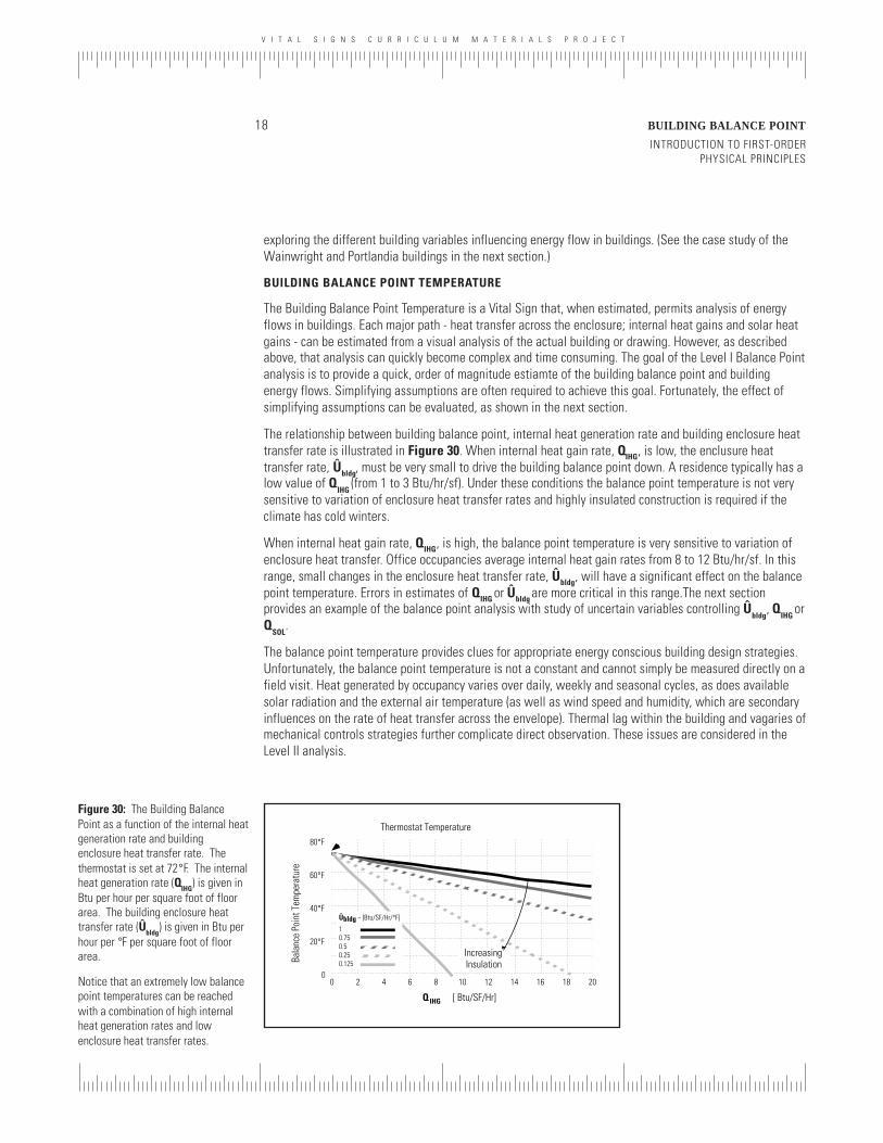
Figure 30: The Building BalancePoint as a function of the internal heatgeneration rate and buildingenclosure heat transfer rate. Thethermostat is set at 72°F. The internalheat generation rate (QIHG) is given inBtu per hour per square foot of floorarea. The building enclosure heattransfer rate (Ûbldg) is given in Btu perhour per °F per square foot of floorarea.
Notice that an extremely low balancepoint temperatures can be reachedwith a combination of high internalheat generation rates and lowenclosure heat transfer rates.
exploring the different building variables influencing energy flow in buildings. (See the case study of theWainwright and Portlandia buildings in the next section.)
BUILDING BALANCE POINT TEMPERATURE
The Building Balance Point Temperature is a Vital Sign that, when estimated, permits analysis of energyflows in buildings. Each major path - heat transfer across the enclosure; internal heat gains and solar heatgains - can be estimated from a visual analysis of the actual building or drawing. However, as describedabove, that analysis can quickly become complex and time consuming. The goal of the Level I Balance Pointanalysis is to provide a quick, order of magnitude estiamte of the building balance point and buildingenergy flows. Simplifying assumptions are often required to achieve this goal. Fortunately, the effect ofsimplifying assumptions can be evaluated, as shown in the next section.
The relationship between building balance point, internal heat generation rate and building enclosure heattransfer rate is illustrated in Figure 30. When internal heat gain rate, QIHG, is low, the enclusure heattransfer rate, Ûbldg, must be very small to drive the building balance point down. A residence typically has alow value of Q
IHG (from 1 to 3 Btu/hr/sf). Under these conditions the balance point temperature is not very
sensitive to variation of enclosure heat transfer rates and highly insulated construction is required if theclimate has cold winters.
When internal heat gain rate, QIHG, is high, the balance point temperature is very sensitive to variation ofenclosure heat transfer. Office occupancies average internal heat gain rates from 8 to 12 Btu/hr/sf. In thisrange, small changes in the enclosure heat transfer rate, Ûbldg, will have a significant effect on the balancepoint temperature. Errors in estimates of QIHG or Ûbldg are more critical in this range.The next sectionprovides an example of the balance point analysis with study of uncertain variables controlling Û
bldg, Q
IHG or
QSOL
.
The balance point temperature provides clues for appropriate energy conscious building design strategies.Unfortunately, the balance point temperature is not a constant and cannot simply be measured directly on afield visit. Heat generated by occupancy varies over daily, weekly and seasonal cycles, as does availablesolar radiation and the external air temperature (as well as wind speed and humidity, which are secondaryinfluences on the rate of heat transfer across the envelope). Thermal lag within the building and vagaries ofmechanical controls strategies further complicate direct observation. These issues are considered in theLevel II analysis.
0 2 4 6 8 10 12 14 16 18 200
20°F
40°F
60°F
80°F
Q IHG [ Btu/SF/Hr]
Bala
nce
Poin
t Tem
pera
ture
Ûbldg ~ [Btu/SF/Hr/°F]
1 0.75 0.5 0.25 0.125
Thermostat Temperature
Increasing Insulation
V I T A L S I G N S C U R R I C U L U M M A T E R I A L S P R O J E C T
19 BUILDING BALANCE POINT
THE BALANCE POINT AND ARCHITECTURAL DESIGN
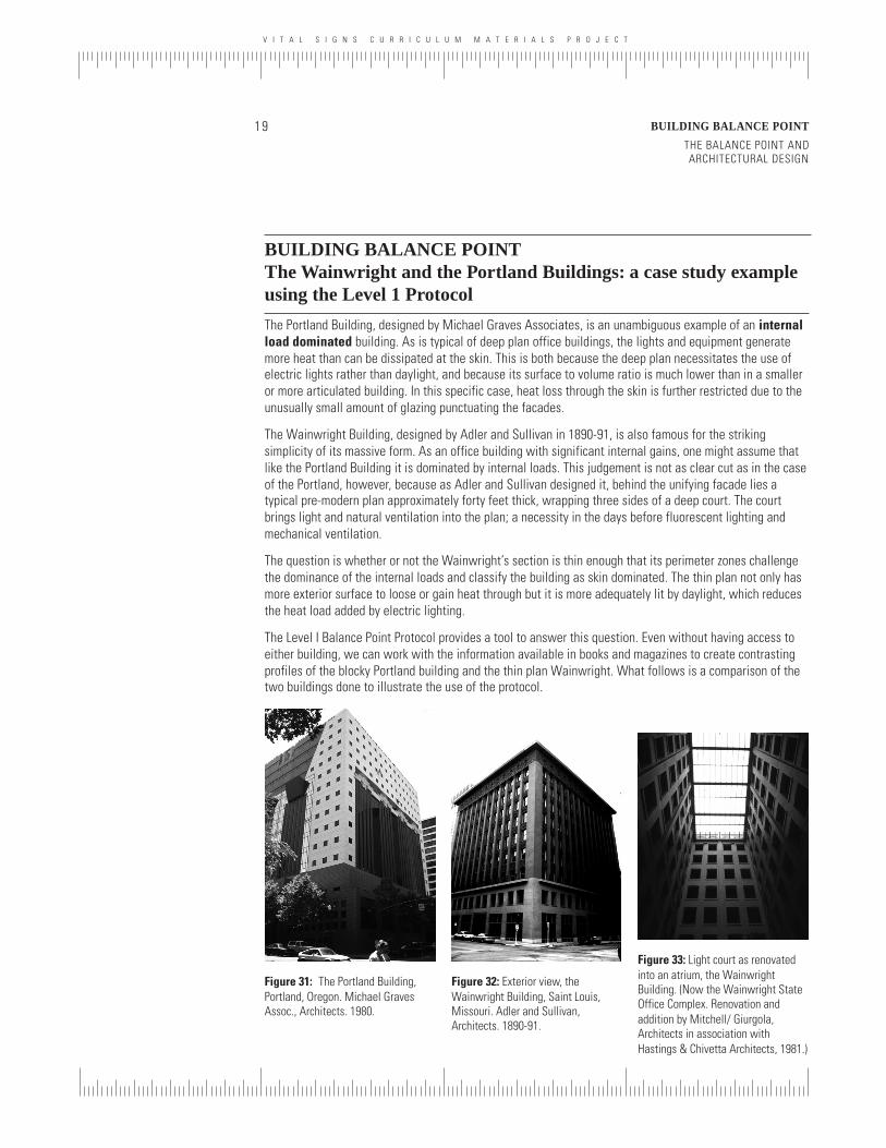
The Portland Building, designed by Michael Graves Associates, is an unambiguous example of an internalload dominated building. As is typical of deep plan office buildings, the lights and equipment generatemore heat than can be dissipated at the skin. This is both because the deep plan necessitates the use ofelectric lights rather than daylight, and because its surface to volume ratio is much lower than in a smalleror more articulated building. In this specific case, heat loss through the skin is further restricted due to theunusually small amount of glazing punctuating the facades.
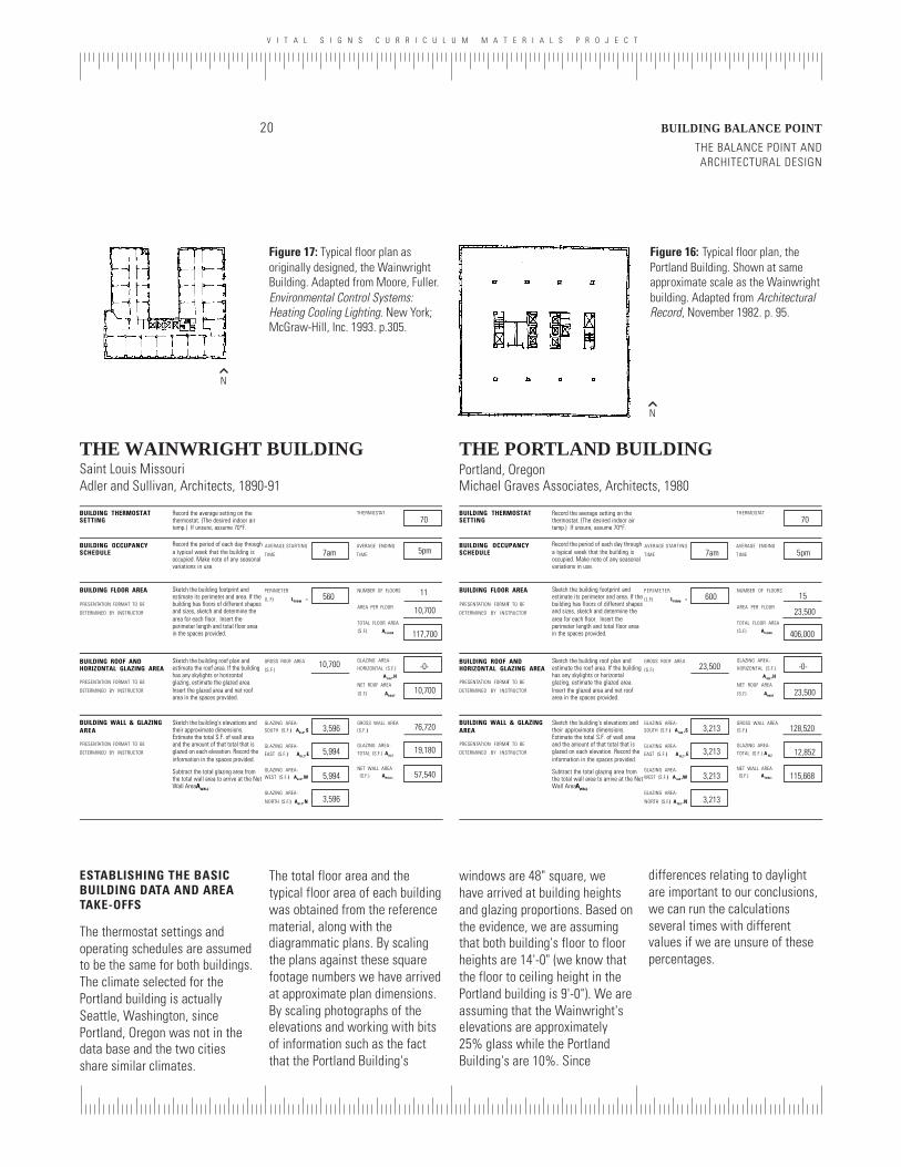
The Wainwright Building, designed by Adler and Sullivan in 1890-91, is also famous for the strikingsimplicity of its massive form. As an office building with significant internal gains, one might assume thatlike the Portland Building it is dominated by internal loads. This judgement is not as clear cut as in the caseof the Portland, however, because as Adler and Sullivan designed it, behind the unifying facade lies atypical pre-modern plan approximately forty feet thick, wrapping three sides of a deep court. The courtbrings light and natural ventilation into the plan; a necessity in the days before fluorescent lighting andmechanical ventilation.
The question is whether or not the Wainwright’s section is thin enough that its perimeter zones challengethe dominance of the internal loads and classify the building as skin dominated. The thin plan not only hasmore exterior surface to loose or gain heat through but it is more adequately lit by daylight, which reducesthe heat load added by electric lighting.
The Level I Balance Point Protocol provides a tool to answer this question. Even without having access toeither building, we can work with the information available in books and magazines to create contrastingprofiles of the blocky Portland building and the thin plan Wainwright. What follows is a comparison of thetwo buildings done to illustrate the use of the protocol.
Figure 32: Exterior view, theWainwright Building, Saint Louis,Missouri. Adler and Sullivan,Architects. 1890-91.
Figure 31: The Portland Building,Portland, Oregon. Michael GravesAssoc., Architects. 1980.
BUILDING BALANCE POINTThe Wainwright and the Portland Buildings: a case study exampleusing the Level 1 Protocol
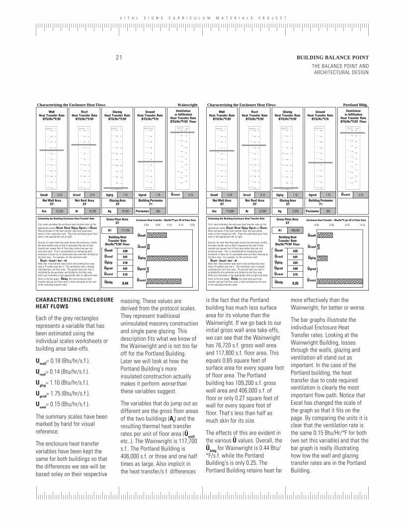
Figure 33: Light court as renovatedinto an atrium, the WainwrightBuilding. (Now the Wainwright StateOffice Complex. Renovation andaddition by Mitchell/ Giurgola,Architects in association withHastings & Chivetta Architects, 1981.)
V I T A L S I G N S C U R R I C U L U M M A T E R I A L S P R O J E C T
THE BALANCE POINT ANDARCHITECTURAL DESIGN
BUILDING BALANCE POINT20
THE WAINWRIGHT BUILDINGSaint Louis MissouriAdler and Sullivan, Architects, 1890-91
THE PORTLAND BUILDINGPortland, OregonMichael Graves Associates, Architects, 1980
Record the average setting on thethermostat. (The desired indoor airtemp.) If unsure, assume 70°F.
Record the period of each day througha typical week that the building isoccupied. Make note of any seasonalvariations in use.
Sketch the building footprint andestimate its perimeter and area. If thebuilding has floors of different shapesand sizes, sketch and determine thearea for each floor. Insert theperimeter length and total floor areain the spaces provided.
Sketch the building roof plan andestimate the roof area. If the buildinghas any skylights or horizontalglazing, estimate the glazed area.Insert the glazed area and net roofarea in the spaces provided.
Sketch the building's elevations andtheir approximate dimensions.Estimate the total S.F. of wall areaand the amount of that total that isglazed on each elevation. Record theinformation in the spaces provided.
Subtract the total glazing area fromthe total wall area to arrive at the NetWall Area AWALL .
BUILDING THERMOSTATSETTING
BUILDING OCCUPANCYSCHEDULE
BUILDING FLOOR AREA
PRESENTATION FORMAT TO BE
DETERMINED BY INSTRUCTOR
BUILDING ROOF ANDHORIZONTAL GLAZING AREA
PRESENTATION FORMAT TO BE
DETERMINED BY INSTRUCTOR
BUILDING WALL & GLAZINGAREA
PRESENTATION FORMAT TO BE
DETERMINED BY INSTRUCTOR
AVERAGE ENDING
TIME
AVERAGE STARTING
TIME
GLAZING AREA-SOUTH (S.F.) A GLZ ,S
GLAZING AREA-
EAST (S.F.) A GLZ , E
GLAZING AREA-WEST (S.F.) A GLZ ,W
GLAZING AREA-
NORTH (S.F.) A GLZ ,N
GROSS WALL AREA(S.F.)
GLAZING AREA-
TOTAL (S.F.) A GLZ
NET WALL AREA (S.F.) A WALL
NUMBER OF FLOORS
AREA PER FLOOR
TOTAL FLOOR AREA
(S.F.) AFLOOR
GROSS ROOF AREA
(S.F.)
P E R I M E T E R
(L.F.) LPERIM =
GLAZING AREA-
HORIZONTAL (S.F.)
A GLZ ,H
NET ROOF AREA
(S.F.) AROOF
THERMOSTAT
70
5pm 7am
600 15
23,500
406,000
23,500 -0-
23,500
3,213
3,213
3,213
3,213
128,520
12,852
115,668
Record the average setting on thethermostat. (The desired indoor airtemp.) If unsure, assume 70°F.
Record the period of each day througha typical week that the building isoccupied. Make note of any seasonalvariations in use.
Sketch the building footprint andestimate its perimeter and area. If thebuilding has floors of different shapesand sizes, sketch and determine thearea for each floor. Insert theperimeter length and total floor areain the spaces provided.
Sketch the building roof plan andestimate the roof area. If the buildinghas any skylights or horizontalglazing, estimate the glazed area.Insert the glazed area and net roofarea in the spaces provided.
Sketch the building's elevations andtheir approximate dimensions.Estimate the total S.F. of wall areaand the amount of that total that isglazed on each elevation. Record theinformation in the spaces provided.
Subtract the total glazing area fromthe total wall area to arrive at the NetWall Area AWALL .
BUILDING THERMOSTATSETTING
BUILDING OCCUPANCYSCHEDULE
BUILDING FLOOR AREA
PRESENTATION FORMAT TO BE
DETERMINED BY INSTRUCTOR
BUILDING ROOF ANDHORIZONTAL GLAZING AREA
PRESENTATION FORMAT TO BE
DETERMINED BY INSTRUCTOR
BUILDING WALL & GLAZINGAREA
PRESENTATION FORMAT TO BE
DETERMINED BY INSTRUCTOR
AVERAGE ENDING
TIME
AVERAGE STARTING
TIME
GLAZING AREA-SOUTH (S.F.) AGLZ, S
GLAZING AREA-
EAST (S.F.) AGLZ, E
GLAZING AREA-WEST (S.F.) AGLZ, W
GLAZING AREA-
NORTH (S.F.) AGLZ, N
GROSS WALL AREA(S.F.)
GLAZING AREA-
TOTAL (S.F.) AGLZ
NET WALL AREA (S.F.) AW A L L
NUMBER OF FLOORS
AREA PER FLOOR
TOTAL FLOOR AREA
(S.F.) AFLOOR
GROSS ROOF AREA
(S.F. )
PERIMETER
(L.F.) LPERIM =
GLAZING AREA-
HORIZONTAL (S.F.)
A GLZ, H
NET ROOF AREA
(S.F.) AROOF
THERMOSTAT
70
5pm 7am
560 11
10,700
117,700
10,700 -0-
10,700
3,596
5,994
5,994
3,596
76,720
19,180
57,540
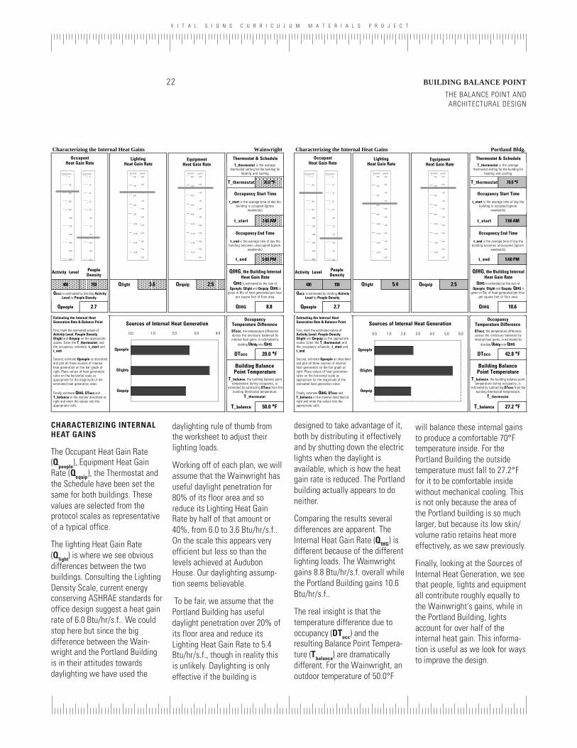
ESTABLISHING THE BASICBUILDING DATA AND AREATAKE-OFFS
The thermostat settings andoperating schedules are assumedto be the same for both buildings.The climate selected for thePortland building is actuallySeattle, Washington, sincePortland, Oregon was not in thedata base and the two citiesshare similar climates.
The total floor area and thetypical floor area of each buildingwas obtained from the referencematerial, along with thediagrammatic plans. By scalingthe plans against these squarefootage numbers we have arrivedat approximate plan dimensions.By scaling photographs of theelevations and working with bitsof information such as the factthat the Portland Building's
windows are 48" square, wehave arrived at building heightsand glazing proportions. Based onthe evidence, we are assumingthat both building's floor to floorheights are 14'-0" (we know thatthe floor to ceiling height in thePortland building is 9'-0"). We areassuming that the Wainwright'selevations are approximately25% glass while the PortlandBuilding's are 10%. Since
Figure 17: Typical floor plan asoriginally designed, the WainwrightBuilding. Adapted from Moore, Fuller.Environmental Control Systems:Heating Cooling Lighting. New York;McGraw-Hill, Inc. 1993. p.305.
Figure 16: Typical floor plan, thePortland Building. Shown at sameapproximate scale as the Wainwrightbuilding. Adapted from ArchitecturalRecord, November 1982. p. 95.
differences relating to daylightare important to our conclusions,we can run the calculationsseveral times with differentvalues if we are unsure of thesepercentages.
N
N
V I T A L S I G N S C U R R I C U L U M M A T E R I A L S P R O J E C T
21 BUILDING BALANCE POINT
THE BALANCE POINT AND ARCHITECTURAL DESIGN
Characterizing the Enclosure Heat Flows Portland Bldg.
Uwall 0.18 Uroof 0.14 Uglzg 1.10 Ugrnd 1.75 0.15
Aw 115,668 Ar 23,500 Ag 12,852 Perimeter 600
Af 406,000
0.05
0.01
0.03
0.00
0.15
0.25
WallHeat Transfer Rate
BTU/Hr/°°°°F/SF
RoofHeat Transfer Rate
BTU/Hr/°°°°F/SF
GlazingHeat Transfer Rate
BTU/Hr/°°°°F/SF
GroundHeat Transfer Rate
BTU/Hr/°°°°F/ft
Ventilationor Infiltration
Heat Transfer RateBTU/Hr/°°°°F/SF Floor
Net Wall AreaSF
Net Roof AreaSF
Glazing AreaSF
Building PerimeterF t
Gross Floor AreaSF
Building HeatTransfer Rate
Btu/Hr/°°°°F/SF Floor
0.00
0.20
0.15
0.30
0.25
0.40
0.35
0.50
0.45
0.10
0.05
Btu/Hr/SF/°F∞
5
6.7
3.3
4
2.5
2.8
2
2.2
10
20
R 0.00
0.20
0.15
0.30
0.25
0.40
0.35
0.50
0.45
0.10
0.05
Btu/Hr/SF/°F∞
5
6.7
3.3
4
2.5
2.8
2
2.2
10
20
R 0.00
0.40
0.30
0.60
0.50
0.80
0.70
1.00
0.90
0.20
0.10
Btu/Hr/SF/°F∞
2.5
3.33
1.67
2
1.25
1.43
1
1.11
5
10
R
0.00
1.20
0.90
1.80
1.50
2.40
2.10
3.00
2.70
0.60
0.30
Btu/Hr/°F per Foot0.00
1.00
0.75
1.50
1.25
2.00
1.75
2.25
0.50
0.25
Btu/Hr/SF/°F cfm/SF 0.00
1.00
0.75
1.50
1.25
2.00
1.75
2.50
2.25
0.50
0.25
0.00 0.05 0.10 0.15
Ûwall
Ûroof
Ûglzg
Ûgrnd
Ûvent
Ûwall
Ûroof
Ûglzg
Ûgrnd
Ûvent
Ûvent
Ûbldg
Estimating the Building Enclosure Heat Transfer Rate
First, mark estimates the enclosure heat transfer rates on the appropriate scales (Uwall, Uroof, Uglzg, Ugrnd and Ûvent). Note estimates of the heat transfer rates and associated areas in their respective cells. Place the estimated gross floor area in the appropriate cell at right.
Second, for each heat flow path across the enclosure, modify the heat transfer rate so that it represents the rate of heat transfer per square foot of floor area rather than per unit enclosure area. This is acomplished by multiplying each enclosure U factor by its associated area and then dividing by the floor area. For example, for the enclosure wall: Ûwall = (Uwall X Aw) ÷ Af Note that heat transfer rates tied to the building floor area have a ^ symbol over the U. The ventilation rate is already estimated per unit floor area. The ground heat loss rate is multiplied by the perimeter and divided by the floor area. Enter your estimates in the appropriate cells at right and mark them on the bar graph. Ûbldg, the total enclosure heat transfer rate per unit floor area, is then estimated as the sum of the individual transfer rates.
Enclosure Heat Transfer ~ Btu/Hr/°°°°F per SF of Floor Area
Characterizing the Enclosure Heat Flows Wainwright
Uwall 0.18 Uroof 0.14 Uglzg 1.10 Ugrnd 1.75 0.15
Aw 57,520 Ar 10,700 Ag 19,180 Perimeter 560
Af 117,700
0.09
0.01
0.18
0.01
0.15
0.44
WallHeat Transfer Rate
BTU/Hr/°°°°F/SF
RoofHeat Transfer Rate
BTU/Hr/°°°°F/SF
GlazingHeat Transfer Rate
BTU/Hr/°°°°F/SF
GroundHeat Transfer Rate
BTU/Hr/°°°°F/ft
Ventilationor Infiltration
Heat Transfer RateBTU/Hr/°°°°F/SF Floor
Net Wall AreaSF
Net Roof AreaSF
Glazing AreaSF
Building PerimeterF t
Gross Floor AreaSF
Building HeatTransfer Rate
Btu/Hr/°°°°F/SF Floor
0.00
0.20
0.15
0.30
0.25
0.40
0.35
0.50
0.45
0.10
0.05
Btu/Hr/SF/°F∞
5
6.7
3.3
4
2.5
2.8
2
2.2
10
20
R 0.00
0.20
0.15
0.30
0.25
0.40
0.35
0.50
0.45
0.10
0.05
Btu/Hr/SF/°F∞
5
6.7
3.3
4
2.5
2.8
2
2.2
10
20
R 0.00
0.40
0.30
0.60
0.50
0.80
0.70
1.00
0.90
0.20
0.10
Btu/Hr/SF/°F∞
2.5
3.33
1.67
2
1.25
1.43
1
1.11
5
10
R
0.00
1.20
0.90
1.80
1.50
2.40
2.10
3.00
2.70
0.60
0.30
Btu/Hr/°F per Foot0.00
1.00
0.75
1.50
1.25
2.00
1.75
2.25
0.50
0.25
Btu/Hr/SF/°F cfm/SF 0.00
1.00
0.75
1.50
1.25
2.00
1.75
2.50
2.25
0.50
0.25
0.00 0.05 0.10 0.15 0.20
Ûwall
Ûroof
Ûglzg
Ûgrnd
Ûvent
Ûwall
Ûroof
Ûglzg
Ûgrnd
Ûvent
Ûvent
Ûbldg
Estimating the Building Enclosure Heat Transfer Rate
First, mark estimates the enclosure heat transfer rates on the appropriate scales (Uwall, Uroof, Uglzg, Ugrnd and Ûvent). Note estimates of the heat transfer rates and associated areas in their respective cells. Place the estimated gross floor area in the appropriate cell at right.
Second, for each heat flow path across the enclosure, modify the heat transfer rate so that it represents the rate of heat transfer per square foot of floor area rather than per unit enclosure area. This is acomplished by multiplying each enclosure U factor by its associated area and then dividing by the floor area. For example, for the enclosure wall: Ûwall = (Uwall X Aw) ÷ Af Note that heat transfer rates tied to the building floor area have a ^ symbol over the U. The ventilation rate is already estimated per unit floor area. The ground heat loss rate is multiplied by the perimeter and divided by the floor area. Enter your estimates in the appropriate cells at right and mark them on the bar graph. Ûbldg, the total enclosure heat transfer rate per unit floor area, is then estimated as the sum of the individual transfer rates.
Enclosure Heat Transfer ~ Btu/Hr/°°°°F per SF of Floor Area
CHARACTERIZING ENCLOSUREHEAT FLOWS
Each of the grey rectanglesrepresents a variable that hasbeen estimated using theindividual scales worksheets orbuilding area take-offs.
Uwall= 0.18 (Btu/hr/s.f.).
Uroof= 0.14 (Btu/hr/s.f.).
Uglzg= 1.10 (Btu/hr/s.f.).
Ugrnd= 1.75 (Btu/hr/s.f.).
Uvent
= 0.15 (Btu/hr/s.f.).
The summary scales have beenmarked by hand for visualreference.
The enclosure heat transfervariables have been kept thesame for both buildings so thatthe differences we see will bebased soley on their respective
massing. These values arederived from the protocol scales.They represent traditionaluninsulated masonry constructionand single pane glazing. Thisdescription fits what we know ofthe Wainwright and is not too faroff for the Portland Building.Later we will look at how thePortland Building's moreinsulated construction actuallymakes it perform worse thanthese variables suggest.
The variables that do jump out asdifferent are the gross floor areasof the two buildings (Af) and theresulting thermal heat transferrates per unit of floor area (Ûwalletc..). The Wainwright is 117,700s.f.. The Portland Building is406,000 s.f. or three and one halftimes as large. Also implicit inthe heat transfer/s.f. differences
is the fact that the Portlandbuilding has much less surfacearea for its volume than theWainwright. If we go back to ourinitial gross wall area take-offs,we can see that the Wainwrighthas 76,720 s.f. gross wall areaand 117,800 s.f. floor area. Thisequals 0.65 square feet ofsurface area for every square footof floor area. The Portlandbuilding has 109,200 s.f. grosswall area and 406,000 s.f. offloor or only 0.27 square feet ofwall for every square foot offloor. That's less than half asmuch skin for its size.
The effects of this are evident inthe various Û values. Overall, theÛbldg for Wainwright is 0.44 Btu/°F/s.f. while the PortlandBuilding's is only 0.25. ThePortland Building retains heat far
more effectively than theWainwright, for better or worse.
The bar graphs illustrate theindividual Enclosure HeatTransfer rates. Looking at theWainwright Building, lossesthrough the walls, glazing andventilation all stand out asimportant. In the case of thePortland building, the heattransfer due to code requiredventilation is clearly the mostimportant flow path. Notice thatExcel has changed the scale ofthe graph so that it fits on thepage. By comparing the units it isclear that the ventilation rate isthe same 0.15 Btu/Hr/°F for both(we set this variable) and that thebar graph is really illustratinghow low the wall and glazingtransfer rates are in the PortlandBuilding.
V I T A L S I G N S C U R R I C U L U M M A T E R I A L S P R O J E C T
THE BALANCE POINT ANDARCHITECTURAL DESIGN
BUILDING BALANCE POINT22
Characterizing the Internal Heat Gains Wainwright
T_thermostat 70.0 °°°°F
t_start 7:00 AM
t_end 5:00 PM
Activity Level People Density
400 150 Qlight 3.6 Qequip 2.5
Qpeople 2.7 QIHG 8.8
DTocc 20.0 °°°°F
T_balance 50.0 °°°°F
OccupantHeat Gain Rate
LightingHeat Gain Rate
EquipmentHeat Gain Rate
Thermostat & Schedule
Occupancy Start Time
Occupancy End Time
QIHG, the Building InternalHeat Gain Rate
OccupancyTemperature DifferenceSources of Internal Heat Generation
0.0 1.0 2.0 3.0 4.0
Qpeople
Qlights
Qequip
0
800
600
1200
1000
1600
1400
2000
1800
400
200
Btu/Person/Hr0
80
60
120
100
160
140
200
180
40
20
SF per Person0.00
2.00
1.50
3.00
2.50
4.00
3.50
5.00
4.50
1.00
0.50
Btu/Hr/SF watt/SF
0.00
8.00
6.00
12 .00
10 .00
16 .00
14 .00
4.00
2.00
0.00
2.00
1.50
3.00
2.50
4.00
3.50
5.00
4.50
1.00
0.50
Btu/Hr/SF watt/SF
0.00
8.00
6.00
12 .00
10 .00
16 .00
14 .00
4.00
2.00
Building Balance Point Temperature
QIHG is estimated as the sum of Qpeople, Qlight and Qequip. QIHG is
given in Btu of heat generated per hour per square foot of floor area.
DTocc, the temperature difference across the enclosure balanced by internal heat gains, is estimated by
dividing Ubldg into QIHG.
T_thermostat is the average thermostat setting for the building for
heating and cooling.
t_start is the average time of day the building is occupied (ignore
weekends).
t_end is the average time of day the building becomes unoccupied (ignore
weekends).
T_balance, the building balance point temperature during occupancy, is
estimated by subtracting DTocc from thebuilding thermostat temperature,
T_thermostat.
Qocc is estimated by dividing Activity Level by People Density.
Estimating the Internal Heat Generation Rate & Balance Point
First, mark the estimated values of Activity Level, People Density, Qlight and Qequip on the appropriate scales. Enter the T_thermostat, and the occupancy schedule, t_start and t_end.
Second, estimate Qpeople as describedand plot all three sources of internal heat generation on the bar graph at right. Place values of heat generation rates on the horizontal scale as appropriate for the magnitude of the estimated heat generation rates.
Finally, estimate QIHG, DTocc and T_balance in the manner described at right and enter the values into the appropriate cells.
Characterizing the Internal Heat Gains Portland Bldg.
T_thermostat 70.0 °°°°F
t_start 7:00 AM
t_end 5:00 PM
Activity Level People Density
400 150 Qlight 5.4 Qequip 2.5
Qpeople 2.7 QIHG 10.6
DTocc 42.8 °°°°F
T_balance 27.2 °°°°F
OccupantHeat Gain Rate
LightingHeat Gain Rate
EquipmentHeat Gain Rate
Thermostat & Schedule
Occupancy Start Time
Occupancy End Time
QIHG, the Building InternalHeat Gain Rate
OccupancyTemperature DifferenceSources of Internal Heat Generation
0.0 1.0 2.0 3.0 4.0 5.0 6.0
Qpeople
Qlights
Qequip
0
800
600
1200
1000
1600
1400
2000
1800
400
200
Btu/Person/Hr0
80
60
120
100
160
140
200
180
40
20
SF per Person0.00
2.00
1.50
3.00
2.50
4.00
3.50
5.00
4.50
1.00
0.50
Btu/Hr/SF watt/SF
0.00
8.00
6.00
12 .00
10 .00
16 .00
14 .00
4.00
2.00
0.00
2.00
1.50
3.00
2.50
4.00
3.50
5.00
4.50
1.00
0.50
Btu/Hr/SF watt/SF
0.00
8.00
6.00
12 .00
10 .00
16 .00
14 .00
4.00
2.00
Building Balance Point Temperature
QIHG is estimated as the sum of Qpeople, Qlight and Qequip. QIHG is
given in Btu of heat generated per hour per square foot of floor area.
DTocc, the temperature difference across the enclosure balanced by internal heat gains, is estimated by
dividing Ubldg into QIHG.
T_thermostat is the average thermostat setting for the building for
heating and cooling.
t_start is the average time of day the building is occupied (ignore
weekends).
t_end is the average time of day the building becomes unoccupied (ignore
weekends).
T_balance, the building balance point temperature during occupancy, is
estimated by subtracting DTocc from thebuilding thermostat temperature,
T_thermostat.
Qocc is estimated by dividing Activity Level by People Density.
Estimating the Internal Heat Generation Rate & Balance Point
First, mark the estimated values of Activity Level, People Density, Qlight and Qequip on the appropriate scales. Enter the T_thermostat, and the occupancy schedule, t_start and t_end.
Second, estimate Qpeople as describedand plot all three sources of internal heat generation on the bar graph at right. Place values of heat generation rates on the horizontal scale as appropriate for the magnitude of the estimated heat generation rates.
Finally, estimate QIHG, DTocc and T_balance in the manner described at right and enter the values into the appropriate cells.
CHARACTERIZING INTERNALHEAT GAINS
The Occupant Heat Gain Rate(Q
people), Equipment Heat Gain
Rate (Qequip), the Thermostat andthe Schedule have been set thesame for both buildings. Thesevalues are selected from theprotocol scales as representativeof a typical office.
The lighting Heat Gain Rate(Qlight) is where we see obviousdifferences between the twobuildings. Consulting the LightingDensity Scale, current energyconserving ASHRAE standards foroffice design suggest a heat gainrate of 6.0 Btu/hr/s.f.. We couldstop here but since the bigdifference between the Wain-wright and the Portland Buildingis in their attitudes towardsdaylighting we have used the
daylighting rule of thumb fromthe worksheet to adjust theirlighting loads.
Working off of each plan, we willassume that the Wainwright hasuseful daylight penetration for80% of its floor area and soreduce its Lighting Heat GainRate by half of that amount or40%, from 6.0 to 3.6 Btu/hr/s.f..On the scale this appears veryefficient but less so than thelevels achieved at AudubonHouse. Our daylighting assump-tion seems believable.
To be fair, we assume that thePortland Building has usefuldaylight penetration over 20% ofits floor area and reduce itsLighting Heat Gain Rate to 5.4Btu/hr/s.f., though in reality thisis unlikely. Daylighting is onlyeffective if the building is
designed to take advantage of it,both by distributing it effectivelyand by shutting down the electriclights when the daylight isavailable, which is how the heatgain rate is reduced. The Portlandbuilding actually appears to doneither.
Comparing the results severaldifferences are apparent. TheInternal Heat Gain Rate (QIHG) isdifferent because of the differentlighting loads. The Wainwrightgains 8.8 Btu/hr/s.f. overall whilethe Portland Building gains 10.6Btu/hr/s.f..
The real insight is that thetemperature difference due tooccupancy (DTocc) and theresulting Balance Point Tempera-ture (Tbalance) are dramaticallydifferent. For the Wainwright, anoutdoor temperature of 50.0°F
will balance these internal gainsto produce a comfortable 70°Ftemperature inside. For thePortland Building the outsidetemperature must fall to 27.2°Ffor it to be comfortable insidewithout mechanical cooling. Thisis not only because the area ofthe Portland building is so muchlarger, but because its low skin/volume ratio retains heat moreeffectively, as we saw previously.
Finally, looking at the Sources ofInternal Heat Generation, we seethat people, lights and equipmentall contribute roughly equally tothe Wainwright's gains, while inthe Portland Building, lightsaccount for over half of theinternal heat gain. This informa-tion is useful as we look for waysto improve the design.
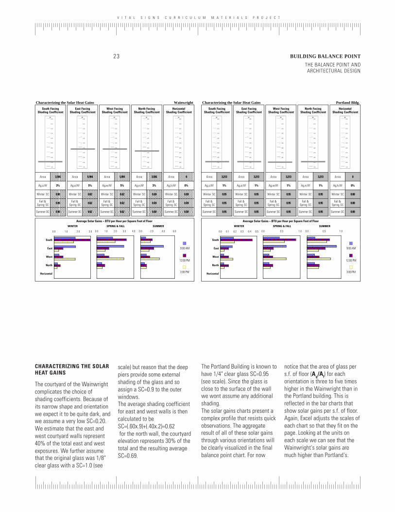
V I T A L S I G N S C U R R I C U L U M M A T E R I A L S P R O J E C T
23 BUILDING BALANCE POINT
THE BALANCE POINT AND ARCHITECTURAL DESIGN
Characterizing the Solar Heat Gains Portland Bldg.
Area 3,213 Area 3,213 Area 3,213 Area 3,213 Area 0
Ag,s/Af 1% Ag,e/Af 1% Ag,w/Af 1% Ag,n/Af 1% Ag,h/Af 0%
Winter SC 0.95 Winter SC 0.95 Winter SC 0.95 Winter SC 0.95 Winter SC 0.00
Fall & Spring SC 0.95 Fall &
Spring SC 0.95 Fall & Spring SC 0.95 Fall &
Spring SC 0.95 Fall & Spring SC 0.00
Summer SC 0.95 Summer SC 0.95 Summer SC 0.95 Summer SC 0.95 Summer SC 0.00
South FacingShading Coefficient
East FacingShading Coefficient
West FacingShading Coefficient
North FacingShading Coefficient
HorizontalShading Coefficient
0.0 0.5 1.0 0.0 0.5 1.0
0.00
0.40
0.30
0.60
0.50
0.80
0.70
1.00
0.90
0.20
0.10
SC0.00
0.40
0.30
0.60
0.50
0.80
0.70
1.00
0.90
0.20
0.10
SC0.00
0.40
0.30
0.60
0.50
0.80
0.70
1.00
0.90
0.20
0.10
SC0.00
0.40
0.30
0.60
0.50
0.80
0.70
1.00
0.90
0.20
0.10
SC0.00
0.40
0.30
0.60
0.50
0.80
0.70
1.00
0.90
0.20
0.10
SC
0.0 0.1 0.2 0.3 0.4 0.5
South
East
West
North
Horizontal
9:00 AM
12:00 PM
3:00 PM
WINTER SPRING & FALL SUMMER
Average Solar Gains ~ BTU per Hour per Square Foot of Floor
Characterizing the Solar Heat Gains Wainwright
Area 3,596 Area 5,994 Area 5,994 Area 3,596 Area 0
Ag,s/Af 3% Ag,e/Af 5% Ag,w/Af 5% Ag,n/Af 3% Ag,h/Af 0%
Winter SC 0.90 Winter SC 0.62 Winter SC 0.62 Winter SC 0.69 Winter SC 0.00
Fall & Spring SC 0.90 Fall &
Spring SC 0.62 Fall & Spring SC 0.62 Fall &
Spring SC 0.69 Fall & Spring SC 0.00
Summer SC 0.90 Summer SC 0.62 Summer SC 0.62 Summer SC 0.69 Summer SC 0.00
South FacingShading Coefficient
East FacingShading Coefficient
West FacingShading Coefficient
North FacingShading Coefficient
HorizontalShading Coefficient
0.0 1.0 2.0 3.0 4.0 0.0 2.0 4.0 6.0
0.00
0.40
0.30
0.60
0.50
0.80
0.70
1.00
0.90
0.20
0.10
SC0.00
0.40
0.30
0.60
0.50
0.80
0.70
1.00
0.90
0.20
0.10
SC0.00
0.40
0.30
0.60
0.50
0.80
0.70
1.00
0.90
0.20
0.10
SC0.00
0.40
0.30
0.60
0.50
0.80
0.70
1.00
0.90
0.20
0.10
SC0.00
0.40
0.30
0.60
0.50
0.80
0.70
1.00
0.90
0.20
0.10
SC
0.0 1.0 2.0 3.0
South
East
West
North
Horizontal
9:00 AM
12:00 PM
3:00 PM
WINTER SPRING & FALL SUMMER
Average Solar Gains ~ BTU per Hour per Square Foot of Floor
CHARACTERIZING THE SOLARHEAT GAINS
The courtyard of the Wainwrightcomplicates the choice ofshading coefficients. Because ofits narrow shape and orientationwe expect it to be quite dark, andwe assume a very low SC=0.20.We estimate that the east andwest courtyard walls represent40% of the total east and westexposures. We further assumethat the original glass was 1/8"clear glass with a SC=1.0 (see
scale) but reason that the deeppiers provide some externalshading of the glass and soassign a SC=0.9 to the outerwindows.The average shading coefficientfor east and west walls is thencalculated to beSC=(.60x.9)+(.40x.2)=0.62 for the north wall, the courtyardelevation represents 30% of thetotal and the resulting averageSC=0.69.
The Portland Building is known tohave 1/4" clear glass SC=0.95(see scale). Since the glass isclose to the surface of the wallwe wont assume any additionalshading.The solar gains charts present acomplex profile that resists quickobservations. The aggregateresult of all of these solar gainsthrough various orientations willbe clearly visualized in the finalbalance point chart. For now
notice that the area of glass pers.f. of floor (Ag/Af) for eachorientation is three to five timeshigher in the Wainwright than inthe Portland building. This isreflected in the bar charts thatshow solar gains per s.f. of floor.Again, Excel adjusts the scales ofeach chart so that they fit on thepage. Looking at the units oneach scale we can see that theWainwright's solar gains aremuch higher than Portland's.
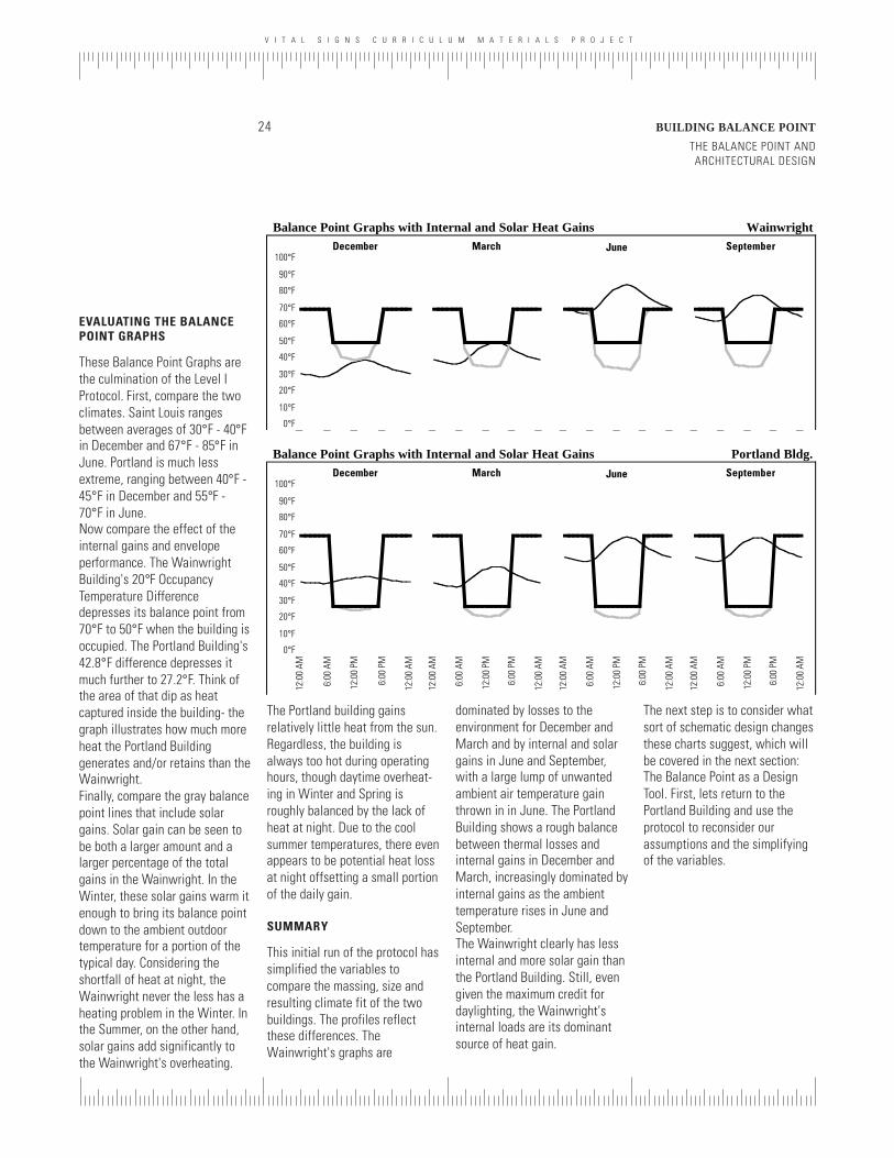
V I T A L S I G N S C U R R I C U L U M M A T E R I A L S P R O J E C T
THE BALANCE POINT ANDARCHITECTURAL DESIGN
BUILDING BALANCE POINT24
EVALUATING THE BALANCEPOINT GRAPHS
These Balance Point Graphs arethe culmination of the Level IProtocol. First, compare the twoclimates. Saint Louis rangesbetween averages of 30°F - 40°Fin December and 67°F - 85°F inJune. Portland is much lessextreme, ranging between 40°F -45°F in December and 55°F -70°F in June.Now compare the effect of theinternal gains and envelopeperformance. The WainwrightBuilding's 20°F OccupancyTemperature Differencedepresses its balance point from70°F to 50°F when the building isoccupied. The Portland Building's42.8°F difference depresses itmuch further to 27.2°F. Think ofthe area of that dip as heatcaptured inside the building- thegraph illustrates how much moreheat the Portland Buildinggenerates and/or retains than theWainwright.Finally, compare the gray balancepoint lines that include solargains. Solar gain can be seen tobe both a larger amount and alarger percentage of the totalgains in the Wainwright. In theWinter, these solar gains warm itenough to bring its balance pointdown to the ambient outdoortemperature for a portion of thetypical day. Considering theshortfall of heat at night, theWainwright never the less has aheating problem in the Winter. Inthe Summer, on the other hand,solar gains add significantly tothe Wainwright's overheating.
The Portland building gainsrelatively little heat from the sun.Regardless, the building isalways too hot during operatinghours, though daytime overheat-ing in Winter and Spring isroughly balanced by the lack ofheat at night. Due to the coolsummer temperatures, there evenappears to be potential heat lossat night offsetting a small portionof the daily gain.
SUMMARY
This initial run of the protocol hassimplified the variables tocompare the massing, size andresulting climate fit of the twobuildings. The profiles reflectthese differences. TheWainwright's graphs are
Balance Point Graphs with Internal and Solar Heat Gains Portland Bldg.
0°F
10°F
20°F
30°F
40°F
50°F
60°F
70°F
80°F
90°F
100°F
12:0
0 AM
6:00
AM
12:0
0 PM
6:00
PM
12:0
0 AM
12:0
0 AM
6:00
AM
12:0
0 PM
6:00
PM
12:0
0 AM
12:0
0 AM
6:00
AM
12:0
0 PM
6:00
PM
12:0
0 AM
12:0
0 AM
6:00
AM
12:0
0 PM
6:00
PM
12:0
0 AM
December March June September
dominated by losses to theenvironment for December andMarch and by internal and solargains in June and September,with a large lump of unwantedambient air temperature gainthrown in in June. The PortlandBuilding shows a rough balancebetween thermal losses andinternal gains in December andMarch, increasingly dominated byinternal gains as the ambienttemperature rises in June andSeptember.The Wainwright clearly has lessinternal and more solar gain thanthe Portland Building. Still, evengiven the maximum credit fordaylighting, the Wainwright'sinternal loads are its dominantsource of heat gain.
Balance Point Graphs with Internal and Solar Heat Gains Wainwright
0°F
10°F
20°F
30°F
40°F
50°F
60°F
70°F
80°F
90°F
100°F
M M M M M M M M M M M M M M M M M M M M
December March June September
The next step is to consider whatsort of schematic design changesthese charts suggest, which willbe covered in the next section:The Balance Point as a DesignTool. First, lets return to thePortland Building and use theprotocol to reconsider ourassumptions and the simplifyingof the variables.
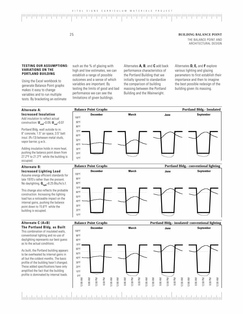
V I T A L S I G N S C U R R I C U L U M M A T E R I A L S P R O J E C T
25 BUILDING BALANCE POINT
THE BALANCE POINT AND ARCHITECTURAL DESIGN
Alternate A:Increased InsulationAdd insulation to reflect actualconstruction: Uwall=0.09, Uroof=0.07
Portland Bldg. wall outside to in:8" concrete, 1.5" air space, 3.5" battinsul. (R=13) between metal studs,vapor barrier, g.w.b..
Adding insulation holds in more heat,pushing the balance point down from27.2°F to 21.3°F while the building isoccupied.
Alternate B:Increased Lighting LoadAssume energy efficient standards forlate 1970's rather than the present.No daylighting. Qlight=8.25 Btu/hr/s.f.
This change also reflects the probableconstruction. Increasing the lightingload has a noticeable impact on theinternal gains, pushing the balancepoint down to 15.6°F while thebuilding is occupied.
Alternate C (A+B)The Portland Bldg. as BuiltThis combination of insulated walls,conventional lighting and no use ofdaylighting represents our best guessas to the actual conditions.
As built, the Portland building appearsto be overheated by internal gains inall but the coldest months. The basicprofile of the building hasn't changed.These added specifications have onlyamplified the fact that the buildingprofile is dominated by internal loads.
TESTING OUR ASSUMPTIONS:VARIATIONS ON THEPORTLAND BUILDING
Using the Excel workbook togenerate Balance Point graphsmakes it easy to changevariables and to run multipletests. By bracketing an estimate
such as the % of glazing withhigh and low estimates, we canestablish a range of possibleoutcomes and a sense of whichvariables are important. Bytesting the limits of good and badperformance we can see thelimitations of given buildings.
Alternates A, B, and C add backperformance characteristics ofthe Portland Building that weinitially ignored to standardizethe comparison of buildingmassing between the PortlandBuilding and the Wainwright.
Balance Point Graphs Portland Bldg.- Insulated
10°F
20°F
30°F
40°F
50°F
60°F
70°F
80°F
90°F
100°FDecember March June September
Balance Point Graphs Portland Bldg.- insulated/ conventional lighting
0°F
10°F
20°F
30°F
40°F
50°F
60°F
70°F
80°F
90°F
100°F
12:0
0 AM
6:00
AM
12:0
0 PM
6:00
PM
12:0
0 AM
12:0
0 AM
6:00
AM
12:0
0 PM
6:00
PM
12:0
0 AM
12:0
0 AM
6:00
AM
12:0
0 PM
6:00
PM
12:0
0 AM
12:0
0 AM
6:00
AM
12:0
0 PM
6:00
PM
12:0
0 AM
December March June September
Balance Point Graphs Portland Bldg.- conventional lighting
10°F
20°F
30°F
40°F
50°F
60°F
70°F
80°F
90°F
100°FDecember March June September
Alternates D, E, and F explorevarious lighting and glazingparameters to first establish theirimportance and then to imaginethe best possible redesign of thebuilding given its massing.
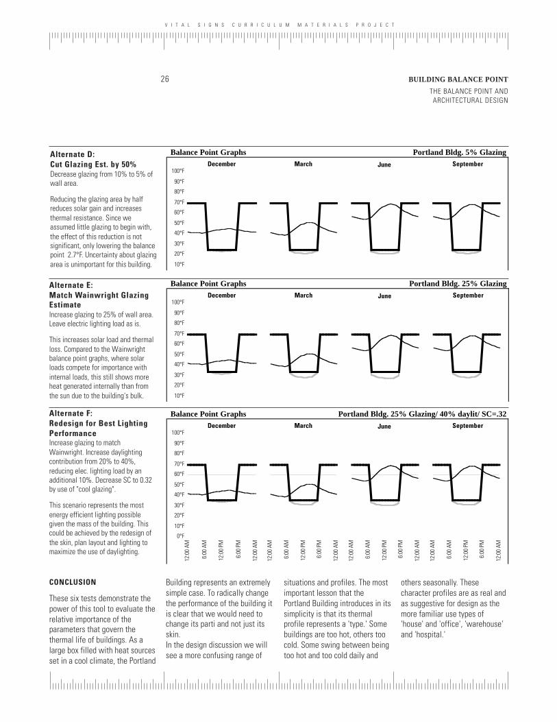
V I T A L S I G N S C U R R I C U L U M M A T E R I A L S P R O J E C T
THE BALANCE POINT ANDARCHITECTURAL DESIGN
BUILDING BALANCE POINT26
Alternate E:Match Wainwright GlazingEstimateIncrease glazing to 25% of wall area.Leave electric lighting load as is.
This increases solar load and thermalloss. Compared to the Wainwrightbalance point graphs, where solarloads compete for importance withinternal loads, this still shows moreheat generated internally than fromthe sun due to the building's bulk.
Alternate D:Cut Glazing Est. by 50%Decrease glazing from 10% to 5% ofwall area.
Reducing the glazing area by halfreduces solar gain and increasesthermal resistance. Since weassumed little glazing to begin with,the effect of this reduction is notsignificant, only lowering the balancepoint 2.7°F. Uncertainty about glazingarea is unimportant for this building.
Alternate F:Redesign for Best LightingPerformanceIncrease glazing to matchWainwright. Increase daylightingcontribution from 20% to 40%,reducing elec. lighting load by anadditional 10%. Decrease SC to 0.32by use of "cool glazing".
This scenario represents the mostenergy efficient lighting possiblegiven the mass of the building. Thiscould be achieved by the redesign ofthe skin, plan layout and lighting tomaximize the use of daylighting.
Balance Point Graphs Portland Bldg. 25% Glazing/ 40% daylit/ SC=.32
0°F
10°F
20°F
30°F
40°F
50°F
60°F
70°F
80°F
90°F
100°F
12:0
0 AM
6:00
AM
12:0
0 PM
6:00
PM
12:0
0 AM
12:0
0 AM
6:00
AM
12:0
0 PM
6:00
PM
12:0
0 AM
12:0
0 AM
6:00
AM
12:0
0 PM
6:00
PM
12:0
0 AM
12:0
0 AM
6:00
AM
12:0
0 PM
6:00
PM
12:0
0 AM
December March June September
Balance Point Graphs Portland Bldg. 25% Glazing
10°F
20°F
30°F
40°F
50°F
60°F
70°F
80°F
90°F
100°FDecember March June September
Balance Point Graphs Portland Bldg. 5% Glazing
10°F
20°F
30°F
40°F
50°F
60°F
70°F
80°F
90°F
100°FDecember March June September
CONCLUSION
These six tests demonstrate thepower of this tool to evaluate therelative importance of theparameters that govern thethermal life of buildings. As alarge box filled with heat sourcesset in a cool climate, the Portland
Building represents an extremelysimple case. To radically changethe performance of the building itis clear that we would need tochange its parti and not just itsskin.In the design discussion we willsee a more confusing range of
situations and profiles. The mostimportant lesson that thePortland Building introduces in itssimplicity is that its thermalprofile represents a 'type.' Somebuildings are too hot, others toocold. Some swing between beingtoo hot and too cold daily and
others seasonally. Thesecharacter profiles are as real andas suggestive for design as themore familiar use types of'house' and 'office', 'warehouse'and 'hospital.'
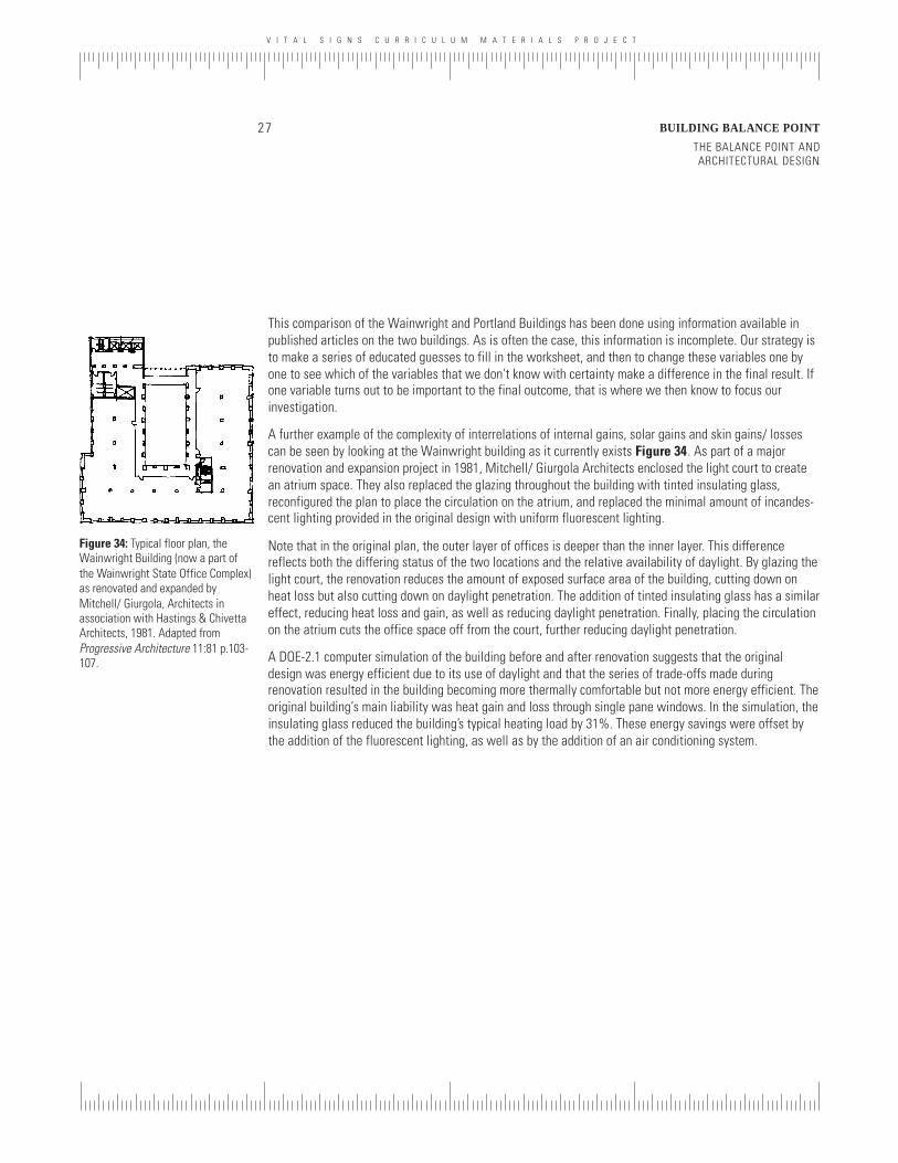
V I T A L S I G N S C U R R I C U L U M M A T E R I A L S P R O J E C T
27 BUILDING BALANCE POINT
THE BALANCE POINT AND ARCHITECTURAL DESIGN
This comparison of the Wainwright and Portland Buildings has been done using information available inpublished articles on the two buildings. As is often the case, this information is incomplete. Our strategy isto make a series of educated guesses to fill in the worksheet, and then to change these variables one byone to see which of the variables that we don't know with certainty make a difference in the final result. Ifone variable turns out to be important to the final outcome, that is where we then know to focus ourinvestigation.
A further example of the complexity of interrelations of internal gains, solar gains and skin gains/ lossescan be seen by looking at the Wainwright building as it currently exists Figure 34. As part of a majorrenovation and expansion project in 1981, Mitchell/ Giurgola Architects enclosed the light court to createan atrium space. They also replaced the glazing throughout the building with tinted insulating glass,reconfigured the plan to place the circulation on the atrium, and replaced the minimal amount of incandes-cent lighting provided in the original design with uniform fluorescent lighting.
Note that in the original plan, the outer layer of offices is deeper than the inner layer. This differencereflects both the differing status of the two locations and the relative availability of daylight. By glazing thelight court, the renovation reduces the amount of exposed surface area of the building, cutting down onheat loss but also cutting down on daylight penetration. The addition of tinted insulating glass has a similareffect, reducing heat loss and gain, as well as reducing daylight penetration. Finally, placing the circulationon the atrium cuts the office space off from the court, further reducing daylight penetration.
A DOE-2.1 computer simulation of the building before and after renovation suggests that the originaldesign was energy efficient due to its use of daylight and that the series of trade-offs made duringrenovation resulted in the building becoming more thermally comfortable but not more energy efficient. Theoriginal building’s main liability was heat gain and loss through single pane windows. In the simulation, theinsulating glass reduced the building’s typical heating load by 31%. These energy savings were offset bythe addition of the fluorescent lighting, as well as by the addition of an air conditioning system.
Figure 34: Typical floor plan, theWainwright Building (now a part ofthe Wainwright State Office Complex)as renovated and expanded byMitchell/ Giurgola, Architects inassociation with Hastings & ChivettaArchitects, 1981. Adapted fromProgressive Architecture 11:81 p.103-107.
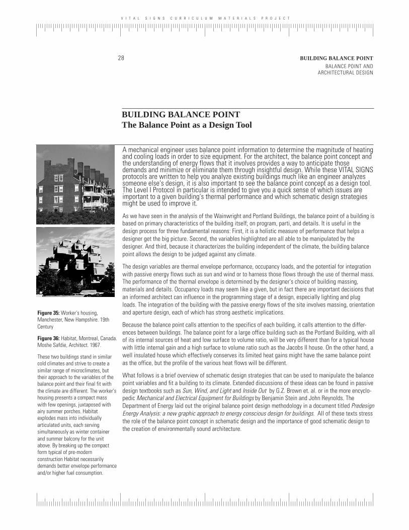
V I T A L S I G N S C U R R I C U L U M M A T E R I A L S P R O J E C T
BALANCE POINT ANDARCHITECTURAL DESIGN
BUILDING BALANCE POINT28
BUILDING BALANCE POINTThe Balance Point as a Design Tool
A mechanical engineer uses balance point information to determine the magnitude of heatingand cooling loads in order to size equipment. For the architect, the balance point concept andthe understanding of energy flows that it involves provides a way to anticipate thosedemands and minimize or eliminate them through insightful design. While these VITAL SIGNSprotocols are written to help you analyze existing buildings much like an engineer analyzessomeone else's design, it is also important to see the balance point concept as a design tool.The Level I Protocol in particular is intended to give you a quick sense of which issues areimportant to a given building's thermal performance and which schematic design strategiesmight be used to improve it.
As we have seen in the analysis of the Wainwright and Portland Buildings, the balance point of a building isbased on primary characteristics of the building itself; on program, parti, and details. It is useful in thedesign process for three fundamental reasons: First, it is a holistic measure of performance that helps adesigner get the big picture. Second, the variables highlighted are all able to be manipulated by thedesigner. And third, because it characterizes the building independent of the climate, the building balancepoint allows the design to be judged against any climate.
The design variables are thermal envelope performance, occupancy loads, and the potential for integrationwith passive energy flows such as sun and wind or to harness those flows through the use of thermal mass.The performance of the thermal envelope is determined by the designer's choice of building massing,materials and details. Occupancy loads may seem like a given, but in fact there are important decisions thatan informed architect can influence in the programming stage of a design, especially lighting and plugloads. The integration of the building with the passive energy flows of the site involves massing, orientationand aperture design, each of which has strong aesthetic implications.
Because the balance point calls attention to the specifics of each building, it calls attention to the differ-ences between buildings. The balance point for a large office building such as the Portland Building, with allof its internal sources of heat and low surface to volume ratio, will be very different than for a typical housewith little internal gain and a high surface to volume ratio such as the Jacobs II house. On the other hand, awell insulated house which effectively conserves its limited heat gains might have the same balance pointas the office, but the profile of the various heat flows will be different.
What follows is a brief overview of schematic design strategies that can be used to manipulate the balancepoint variables and fit a building to its climate. Extended discussions of these ideas can be found in passivedesign textbooks such as Sun, Wind, and Light and Inside Out by G.Z. Brown et. al. or in the more encyclo-pedic Mechanical and Electrical Equipment for Buildings by Benjamin Stein and John Reynolds. TheDepartment of Energy laid out the original balance point design methodology in a document titled PredesignEnergy Analysis: a new graphic approach to energy conscious design for buildings. All of these texts stressthe role of the balance point concept in schematic design and the importance of good schematic design tothe creation of environmentally sound architecture.
Figure 35: Worker's housing,Manchester, New Hampshire. 19thCentury
Figure 36: Habitat, Montreal, Canada.Moshe Safdie, Architect. 1967.
These two buildings stand in similarcold climates and strive to create asimilar range of microclimates, buttheir approach to the variables of thebalance point and their final fit withthe climate are different. The worker'shousing presents a compact masswith few openings, juxtaposed withairy summer porches. Habitatexplodes mass into individuallyarticulated units, each servingsimultaneously as winter containerand summer balcony for the unitabove. By breaking up the compactform typical of pre-modernconstruction Habitat necessarilydemands better envelope performanceand/or higher fuel consumption.
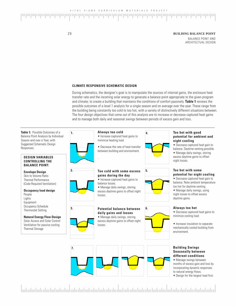
V I T A L S I G N S C U R R I C U L U M M A T E R I A L S P R O J E C T
29 BUILDING BALANCE POINT
BALANCE POINT ANDARCHITECTUAL DESIGN
CLIMATE RESPONSIVE SCHEMATIC DESIGN
During schematics, the designer's goal is to manipulate the sources of internal gains, the enclosure heattransfer rate and the incoming solar energy to generate a balance point appropriate to the given programand climate; to create a building that maintains the conditions of comfort passively. Table 1 reviews thepossible outcomes of a level 1 analysis for a single season and on average over the year. These range fromthe building being constantly too cold to too hot, with a variety of distinctively different situations between.The four design objectives that come out of this analysis are to increase or decrease captured heat gainsand to manage both daily and seasonal swings between periods of excess gain and loss.
DESIGN VARIABLESCONTROLLING THEBALANCE POINT:
Envelope DesignSkin to Volume RatioThermal Performance(Code Required Ventilation)
Occupancy load designPeopleLightsEquipmentOccupancy ScheduleThermostat Setting
Natural Energy Flow DesignSolar Access and Solar ControlVentilation for passive coolingThermal Storage
Table 1: Possible Outcomes of aBalance Point Analysis by IndividualSeason and over a Year, withSuggested Schematic DesignResponses.
Always too cold• Increase captured heat gains tominimize heating load.
• Decrease the rate of heat transferbetween building and environment.
.
Too cold with some excessgains during the day• Increase captured heat gains tobalance losses.• Manage daily swings, storingexcess daytime gains to offset nightlosses.
Potential balance betweendaily gains and losses• Manage daily swings, storingexcess daytime gains to offset nightlosses.
Too hot with goodpotential for ambient andnight cooling• Decrease captured heat gain tobalance. Daytime venting possible.• Manage daily swings, storingexcess daytime gains to offsetnight losses.
Too hot with somepotential for night cooling• Decrease captured heat gain tobalance. Note ambient temperaturetoo hot for daytime venting.• Manage daily swings, usingnight losses to offset excessdaytime gains.
Always too hot• Decrease captured heat gains tominimize cooling load.
• Increase insulation to separatemechanically cooled building fromenvironment.
Building SwingsSeasonally betweendifferent conditions• Manage swings betweenmonths of excess gain and loss byincorporating dynamic responsesto natural energy flows.• Design for the largest load first.
1.
2.
3.
7.
4.
5.
6.
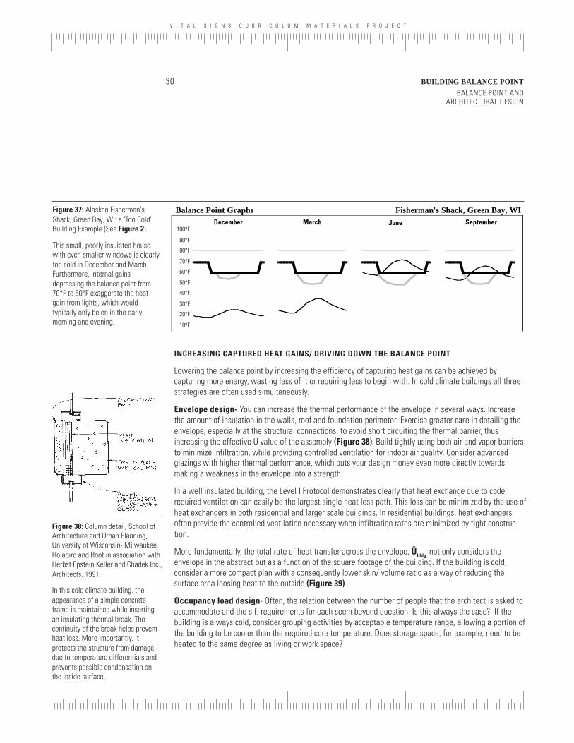
V I T A L S I G N S C U R R I C U L U M M A T E R I A L S P R O J E C T
BALANCE POINT ANDARCHITECTURAL DESIGN
BUILDING BALANCE POINT30
INCREASING CAPTURED HEAT GAINS/ DRIVING DOWN THE BALANCE POINT
Lowering the balance point by increasing the efficiency of capturing heat gains can be achieved bycapturing more energy, wasting less of it or requiring less to begin with. In cold climate buildings all threestrategies are often used simultaneously.
Envelope design- You can increase the thermal performance of the envelope in several ways. Increasethe amount of insulation in the walls, roof and foundation perimeter. Exercise greater care in detailing theenvelope, especially at the structural connections, to avoid short circuiting the thermal barrier, thusincreasing the effective U value of the assembly (Figure 38). Build tightly using both air and vapor barriersto minimize infiltration, while providing controlled ventilation for indoor air quality. Consider advancedglazings with higher thermal performance, which puts your design money even more directly towardsmaking a weakness in the envelope into a strength.
In a well insulated building, the Level I Protocol demonstrates clearly that heat exchange due to coderequired ventilation can easily be the largest single heat loss path. This loss can be minimized by the use ofheat exchangers in both residential and larger scale buildings. In residential buildings, heat exchangersoften provide the controlled ventilation necessary when infiltration rates are minimized by tight construc-tion.
More fundamentally, the total rate of heat transfer across the envelope, Ûbldg, not only considers theenvelope in the abstract but as a function of the square footage of the building. If the building is cold,consider a more compact plan with a consequently lower skin/ volume ratio as a way of reducing thesurface area loosing heat to the outside (Figure 39).
Occupancy load design- Often, the relation between the number of people that the architect is asked toaccommodate and the s.f. requirements for each seem beyond question. Is this always the case? If thebuilding is always cold, consider grouping activities by acceptable temperature range, allowing a portion ofthe building to be cooler than the required core temperature. Does storage space, for example, need to beheated to the same degree as living or work space?
Figure 37: Alaskan Fisherman'sShack, Green Bay, WI: a 'Too Cold'Building Example (See Figure 2).
This small, poorly insulated housewith even smaller windows is clearlytoo cold in December and March.Furthermore, internal gainsdepressing the balance point from70°F to 60°F exaggerate the heatgain from lights, which wouldtypically only be on in the earlymorning and evening.
Figure 38: Column detail, School ofArchitecture and Urban Planning,University of Wisconsin- Milwaukee.Holabird and Root in association withHerbst Epstein Keller and Chadek Inc.,Architects. 1991.
In this cold climate building, theappearance of a simple concreteframe is maintained while insertingan insulating thermal break. Thecontinuity of the break helps preventheat loss. More importantly, itprotects the structure from damagedue to temperature differentials andprevents possible condensation onthe inside surface.
Balance Point Graphs Fisherman's Shack, Green Bay, WI
10°F
20°F
30°F
40°F
50°F
60°F
70°F
80°F
90°F
100°FDecember March June September
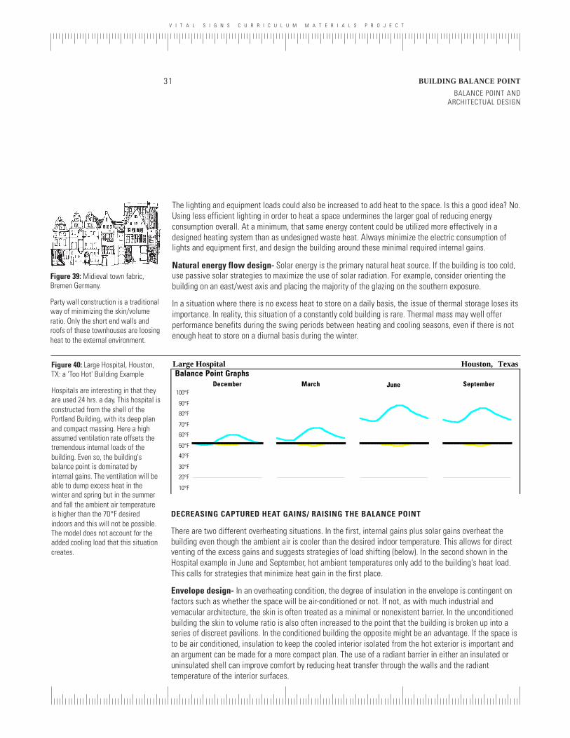
V I T A L S I G N S C U R R I C U L U M M A T E R I A L S P R O J E C T
31 BUILDING BALANCE POINT
BALANCE POINT ANDARCHITECTUAL DESIGN
The lighting and equipment loads could also be increased to add heat to the space. Is this a good idea? No.Using less efficient lighting in order to heat a space undermines the larger goal of reducing energyconsumption overall. At a minimum, that same energy content could be utilized more effectively in adesigned heating system than as undesigned waste heat. Always minimize the electric consumption oflights and equipment first, and design the building around these minimal required internal gains.
Natural energy flow design- Solar energy is the primary natural heat source. If the building is too cold,use passive solar strategies to maximize the use of solar radiation. For example, consider orienting thebuilding on an east/west axis and placing the majority of the glazing on the southern exposure.
In a situation where there is no excess heat to store on a daily basis, the issue of thermal storage loses itsimportance. In reality, this situation of a constantly cold building is rare. Thermal mass may well offerperformance benefits during the swing periods between heating and cooling seasons, even if there is notenough heat to store on a diurnal basis during the winter.
Figure 39: Midieval town fabric,Bremen Germany.
Party wall construction is a traditionalway of minimizing the skin/volumeratio. Only the short end walls androofs of these townhouses are loosingheat to the external environment.
DECREASING CAPTURED HEAT GAINS/ RAISING THE BALANCE POINT
There are two different overheating situations. In the first, internal gains plus solar gains overheat thebuilding even though the ambient air is cooler than the desired indoor temperature. This allows for directventing of the excess gains and suggests strategies of load shifting (below). In the second shown in theHospital example in June and September, hot ambient temperatures only add to the building's heat load.This calls for strategies that minimize heat gain in the first place.
Envelope design- In an overheating condition, the degree of insulation in the envelope is contingent onfactors such as whether the space will be air-conditioned or not. If not, as with much industrial andvernacular architecture, the skin is often treated as a minimal or nonexistent barrier. In the unconditionedbuilding the skin to volume ratio is also often increased to the point that the building is broken up into aseries of discreet pavilions. In the conditioned building the opposite might be an advantage. If the space isto be air conditioned, insulation to keep the cooled interior isolated from the hot exterior is important andan argument can be made for a more compact plan. The use of a radiant barrier in either an insulated oruninsulated shell can improve comfort by reducing heat transfer through the walls and the radianttemperature of the interior surfaces.
Figure 40: Large Hospital, Houston,TX: a 'Too Hot' Building Example
Hospitals are interesting in that theyare used 24 hrs. a day. This hospital isconstructed from the shell of thePortland Building, with its deep planand compact massing. Here a highassumed ventilation rate offsets thetremendous internal loads of thebuilding. Even so, the building'sbalance point is dominated byinternal gains. The ventilation will beable to dump excess heat in thewinter and spring but in the summerand fall the ambient air temperatureis higher than the 70°F desiredindoors and this will not be possible.The model does not account for theadded cooling load that this situationcreates.
Large Hospital Houston, Texas Balance Point Graphs
10°F
20°F
30°F
40°F
50°F
60°F
70°F
80°F
90°F
100°FDecember March June September
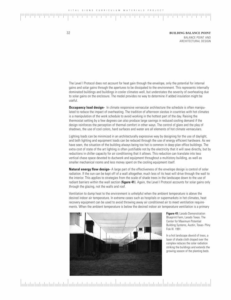
V I T A L S I G N S C U R R I C U L U M M A T E R I A L S P R O J E C T
BALANCE POINT ANDARCHITECTURAL DESIGN
BUILDING BALANCE POINT32
The Level I Protocol does not account for heat gain through the envelope, only the potential for internalgains and solar gains through the apertures to be dissipated to the environment. This represents internallydominated buildings and buildings in cooler climates well, but understates the severity of overheating dueto solar gains on the enclosure. The model provides no way to determine if added insulation might beuseful.
Occupancy load design- In climate responsive vernacular architecture the schedule is often manipu-lated to reduce the impact of overheating. The tradition of afternoon siestas in countries with hot climatesis a manipulation of the work schedule to avoid working in the hottest part of the day. Raising thethermostat setting by a few degrees can also produce large savings in reduced cooling demand if thedesign reinforces the perception of thermal comfort in other ways. The control of glare and the play ofshadows, the use of cool colors, hard surfaces and water are all elements of hot climate vernaculars.
Lighting loads can be minimized in an architecturally expressive way by designing for the use of daylight,and both lighting and equipment loads can be reduced through the use of energy efficient hardware. As wehave seen, the situation of the building always being too hot is common in deep plan office buildings. Theextra cost of state of the art lighting is often justifiable not by the electricity that it will save directly, but byreductions in chiller capacity for air conditioning that it allows. This reduction can translate into lessvertical chase space devoted to ductwork and equipment throughout a multistory building, as well assmaller mechanical rooms and less money spent on the cooling equipment itself.
Natural energy flow design- A large part of the effectiveness of the envelope design is control of solarradiation. If the sun can be kept off of a wall altogether, much less of its heat will drive through the wall tothe interior. This applies to strategies from the scale of shade trees in the landscape down to the use ofradiant barriers within the wall section (figure 41). Again, the Level I Protocol accounts for solar gains onlythrough the glazing, not the walls and roof.
Ventilation to dump heat to the environment is unhelpful when the ambient temperature is above thedesired indoor air temperature. In extreme cases such as hospitals or supermarkets in hot climates, heatrecovery equipment can be used to avoid throwing away air conditioned air to meet ventilation require-ments. When the ambient temperature is below the desired indoor air temperature ventilation is a primary
Figure 41: Larado DemonstrationBlueprint Farm, Larado Texas. TheCenter for Maximum PotentialBuilding Systems, Austin, Texas- PlinyFisk III. 1991.
In a hot landscape devoid of trees, alayer of shade cloth draped over thecomplex reduces the solar radiationstriking the buildings and extends thegrowing season of the planting beds.
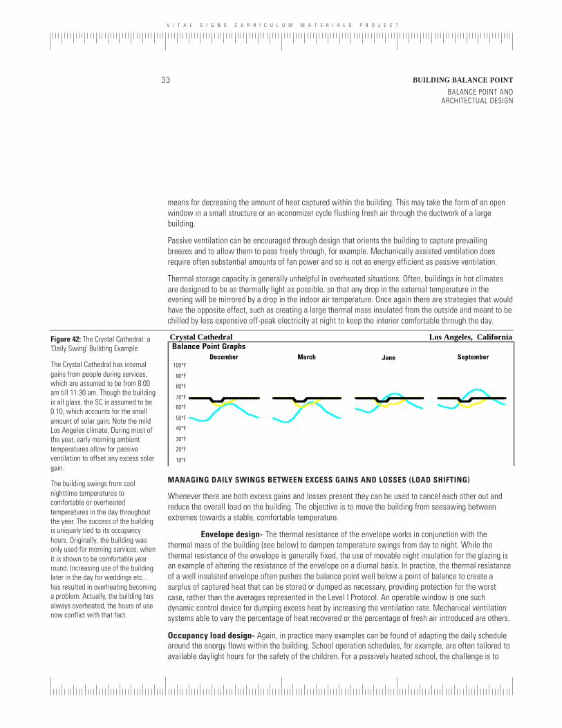
V I T A L S I G N S C U R R I C U L U M M A T E R I A L S P R O J E C T
33 BUILDING BALANCE POINT
BALANCE POINT ANDARCHITECTUAL DESIGN
MANAGING DAILY SWINGS BETWEEN EXCESS GAINS AND LOSSES (LOAD SHIFTING)
Whenever there are both excess gains and losses present they can be used to cancel each other out andreduce the overall load on the building. The objective is to move the building from seesawing betweenextremes towards a stable, comfortable temperature.
Envelope design- The thermal resistance of the envelope works in conjunction with thethermal mass of the building (see below) to dampen temperature swings from day to night. While thethermal resistance of the envelope is generally fixed, the use of movable night insulation for the glazing isan example of altering the resistance of the envelope on a diurnal basis. In practice, the thermal resistanceof a well insulated envelope often pushes the balance point well below a point of balance to create asurplus of captured heat that can be stored or dumped as necessary, providing protection for the worstcase, rather than the averages represented in the Level I Protocol. An operable window is one suchdynamic control device for dumping excess heat by increasing the ventilation rate. Mechanical ventilationsystems able to vary the percentage of heat recovered or the percentage of fresh air introduced are others.
Occupancy load design- Again, in practice many examples can be found of adapting the daily schedulearound the energy flows within the building. School operation schedules, for example, are often tailored toavailable daylight hours for the safety of the children. For a passively heated school, the challenge is to
Figure 42: The Crystal Cathedral: a'Daily Swing' Building Example
The Crystal Cathedral has internalgains from people during services,which are assumed to be from 8:00am till 11:30 am. Though the buildingis all glass, the SC is assumed to be0.10, which accounts for the smallamount of solar gain. Note the mildLos Angeles climate: During most ofthe year, early morning ambienttemperatures allow for passiveventilation to offset any excess solargain.
The building swings from coolnighttime temperatures tocomfortable or overheatedtemperatures in the day throughoutthe year. The success of the buildingis uniquely tied to its occupancyhours. Originally, the building wasonly used for morning services, whenit is shown to be comfortable yearround. Increasing use of the buildinglater in the day for weddings etc...has resulted in overheating becominga problem. Actually, the building hasalways overheated, the hours of usenow conflict with that fact.
means for decreasing the amount of heat captured within the building. This may take the form of an openwindow in a small structure or an economizer cycle flushing fresh air through the ductwork of a largebuilding.
Passive ventilation can be encouraged through design that orients the building to capture prevailingbreezes and to allow them to pass freely through, for example. Mechanically assisted ventilation doesrequire often substantial amounts of fan power and so is not as energy efficient as passive ventilation.
Thermal storage capacity is generally unhelpful in overheated situations. Often, buildings in hot climatesare designed to be as thermally light as possible, so that any drop in the external temperature in theevening will be mirrored by a drop in the indoor air temperature. Once again there are strategies that wouldhave the opposite effect, such as creating a large thermal mass insulated from the outside and meant to bechilled by less expensive off-peak electricity at night to keep the interior comfortable through the day.
Crystal Cathedral Los Angeles, California Balance Point Graphs
10°F
20°F
30°F
40°F
50°F
60°F
70°F
80°F
90°F
100°FDecember March June September
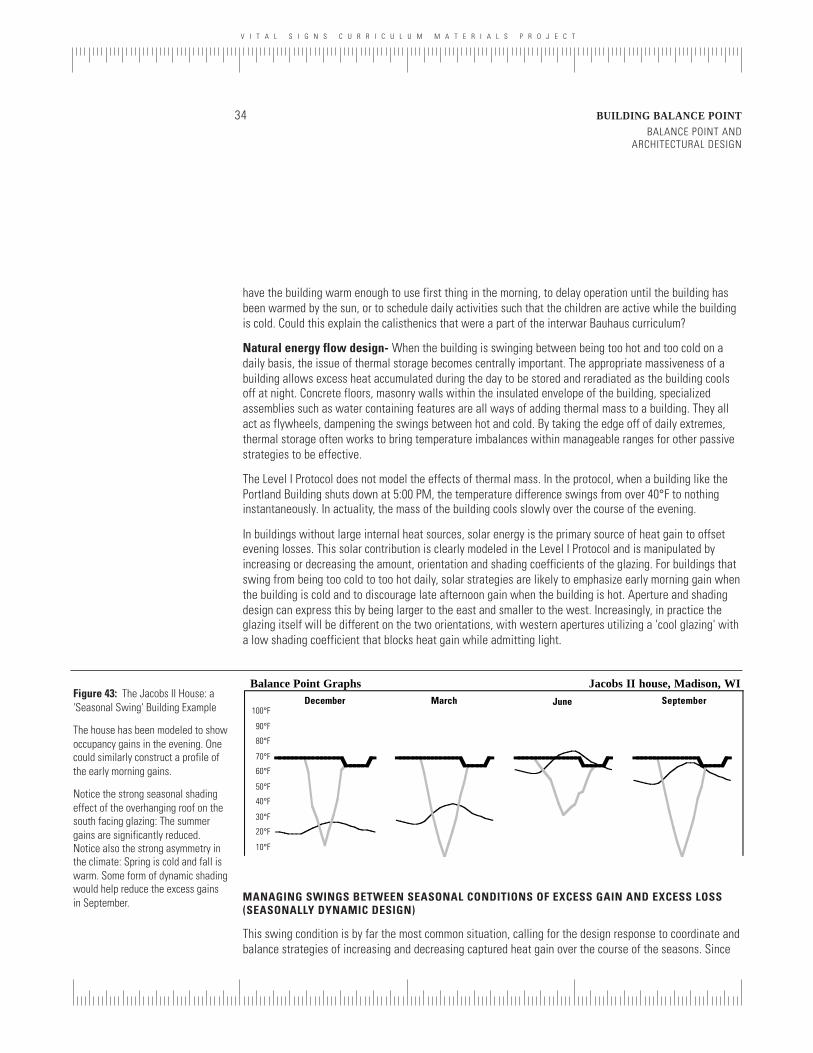
V I T A L S I G N S C U R R I C U L U M M A T E R I A L S P R O J E C T
BALANCE POINT ANDARCHITECTURAL DESIGN
BUILDING BALANCE POINT34
have the building warm enough to use first thing in the morning, to delay operation until the building hasbeen warmed by the sun, or to schedule daily activities such that the children are active while the buildingis cold. Could this explain the calisthenics that were a part of the interwar Bauhaus curriculum?
Natural energy flow design- When the building is swinging between being too hot and too cold on adaily basis, the issue of thermal storage becomes centrally important. The appropriate massiveness of abuilding allows excess heat accumulated during the day to be stored and reradiated as the building coolsoff at night. Concrete floors, masonry walls within the insulated envelope of the building, specializedassemblies such as water containing features are all ways of adding thermal mass to a building. They allact as flywheels, dampening the swings between hot and cold. By taking the edge off of daily extremes,thermal storage often works to bring temperature imbalances within manageable ranges for other passivestrategies to be effective.
The Level I Protocol does not model the effects of thermal mass. In the protocol, when a building like thePortland Building shuts down at 5:00 PM, the temperature difference swings from over 40°F to nothinginstantaneously. In actuality, the mass of the building cools slowly over the course of the evening.
In buildings without large internal heat sources, solar energy is the primary source of heat gain to offsetevening losses. This solar contribution is clearly modeled in the Level I Protocol and is manipulated byincreasing or decreasing the amount, orientation and shading coefficients of the glazing. For buildings thatswing from being too cold to too hot daily, solar strategies are likely to emphasize early morning gain whenthe building is cold and to discourage late afternoon gain when the building is hot. Aperture and shadingdesign can express this by being larger to the east and smaller to the west. Increasingly, in practice theglazing itself will be different on the two orientations, with western apertures utilizing a 'cool glazing' witha low shading coefficient that blocks heat gain while admitting light.
Balance Point Graphs Jacobs II house, Madison, WI
10°F
20°F
30°F
40°F
50°F
60°F
70°F
80°F
90°F
100°FDecember March June September
Figure 43: The Jacobs II House: a'Seasonal Swing' Building Example
The house has been modeled to showoccupancy gains in the evening. Onecould similarly construct a profile ofthe early morning gains.
Notice the strong seasonal shadingeffect of the overhanging roof on thesouth facing glazing: The summergains are significantly reduced.Notice also the strong asymmetry inthe climate: Spring is cold and fall iswarm. Some form of dynamic shadingwould help reduce the excess gainsin September. MANAGING SWINGS BETWEEN SEASONAL CONDITIONS OF EXCESS GAIN AND EXCESS LOSS
(SEASONALLY DYNAMIC DESIGN)
This swing condition is by far the most common situation, calling for the design response to coordinate andbalance strategies of increasing and decreasing captured heat gain over the course of the seasons. Since
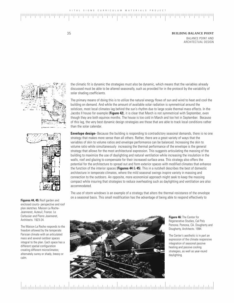
V I T A L S I G N S C U R R I C U L U M M A T E R I A L S P R O J E C T
35 BUILDING BALANCE POINT
BALANCE POINT ANDARCHITECTUAL DESIGN
the climatic fit is dynamic the strategies must also be dynamic, which means that the variables alreadydiscussed must be able to be altered seasonally, such as provided for in the protocol by the variability ofsolar shading coefficients.
The primary means of doing this is to utilize the natural energy flows of sun and wind to heat and cool thebuilding on demand. And while the amount of available solar radiation is symmetrical around thesolstices, most local climates lag behind the sun's rhythm due to large scale thermal mass effects. In theJacobs II house for example (Figure 42), it is clear that March is not symmetrical with September, eventhough they are both equinox months. The house is too cold in March and too hot in September. Becauseof this lag, the very best dynamic design strategies are those that are able to track local conditions ratherthan the solar calendar.
Envelope design- Because the building is responding to contradictory seasonal demands, there is no onestrategy that makes more sense than all others. Rather, there are a great variety of ways that thevariables of skin to volume ratios and envelope performance can be balanced. Increasing the skin tovolume ratio while simultaneously increasing the thermal performance of the envelope is the generalstrategy that allows for the most architectural expression. This suggests articulating the massing of thebuilding to maximize the use of daylighting and natural ventilation while increasing the insulation in thewalls, roof and glazing to compensate for their increased surface area. This strategy also offers thepotential for the architecture to spread out and form exterior spaces with modified climates that enhancethe function of the interior spaces (Figures 44 & 45). This in a nutshell describes the best of domesticarchitecture in temperate climates, where the mild seasonal swings inspire variety in massing andconnection to the outdoors. An opposite, more economical approach might seek to keep the massingcompact while insuring that strategies to reduce overheating such as daylighting and ventilation are alsoaccommodated.
The use of storm windows is an example of a strategy that alters the thermal resistance of the envelopeon a seasonal basis. This small modification has the advantage of being able to respond effectively to
Figures 44, 45: Roof garden andenclosed courts- perspective and roofplan sketches. Maison La Roche-Jeanneret, Auteuil, France. LeCorbusier and Pierre Jeanneret,Architects. 1923-24.
The Maison La Roche responds to thefreedom allowed by the temperateParisian climate with an articulatedmass and several outdoor spacesintegral to the plan. Each space has adifferent spatial configurationcreating different microclimates;alternately sunny or shady, breezy orcalm.
Figure 46: The Center forRegenerative Studies, Cal PolyPomona. Pomona, CA. Dougherty andDougherty, Architects. 1994.
The Center's aesthetic is in part anexpression of the climate responsiveintegration of seasonal passiveheating and passive coolingstrategies, as well as year-rounddaylighting.
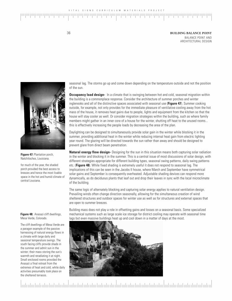
V I T A L S I G N S C U R R I C U L U M M A T E R I A L S P R O J E C T
BALANCE POINT ANDARCHITECTURAL DESIGN
BUILDING BALANCE POINT36
Figure 48: Anasazi cliff dwellings,Mesa Verde, Colorado.
The cliff dwellings of Mesa Verde area paragon example of the passiveharnessing of natural energy flows ina climate with large daily andseasonal temperature swings. Thesouth facing cliffs provide shade inthe summer and admit sun in thewinter; their mass storing the sun'swarmth and reradiating it at night.Small enclosed rooms provided theAnasazi a final retreat from theextremes of heat and cold, while dailyactivities presumably took place onthe sheltered terraces.
seasonal lag. The storms go up and come down depending on the temperature outside and not the positionof the sun.
Occupancy load design- In a climate that is swinging between hot and cold, seasonal migration withinthe building is a commonplace response. Consider the architecture of summer porches and winteringlenooks and all of the distinctive spaces associated with seasonal use (Figure 47). Summer cookingoutside, for example, not only provides for the immediate pleasure of ventilative cooling away from the hotmass of the house, it removes heat gains due to people, lights and equipment from the kitchen so that thehouse will stay cooler as well. Or consider migration strategies within the building, such as where familymembers might gather in an inner core of a house for the winter, shutting off heat to the unused rooms...this is effectively increasing the people loads by decreasing the area of the plan.
Daylighting can be designed to simultaneously provide solar gain in the winter while blocking it in thesummer, providing additional heat in the winter while reducing internal heat gain from electric lightingyear round. The glazing will be directed towards the sun rather than away and should be designed toprevent glare from direct beam penetration.
Natural energy flow design- Designing for the sun in this situation means both capturing solar radiationin the winter and blocking it in the summer. This is a central issue of most discussions of solar design, withdifferent strategies appropriate for different building types, seasonal swing patterns, daily swing patternsetc. (Figure 48). While fixed shading is extremely useful it does not respond to seasonal lag. Theimplications of this can be seen in the Jacobs II house, where March and September have symmetricalsolar gains and September is consequently overheated. Adjustable shading devices can respond moredynamically, as do deciduous plants that leaf out and drop their leaves in sync with the local microclimateof the building.
The same logic of alternately blocking and capturing solar energy applies to natural ventilation design.Prevailing winds often change direction seasonally, allowing for the simultaneous creation of windsheltered structures and outdoor spaces for winter use as well as for structures and external spaces thatare open to summer breezes.
Building mass does not play a role in offsetting gains and losses on a seasonal basis. Some specializedmechanical systems such as large scale ice storage for district cooling may operate with seasonal timelags but even massive buildings heat up and cool down in a matter of days at the most.
Figure 47: Plantation porch,Natchitoches, Louisiana.
for much of the year, the shadedporch provided the best access tobreezes and hence the most livablespace in the hot and humid climate ofcentral Lousiana.
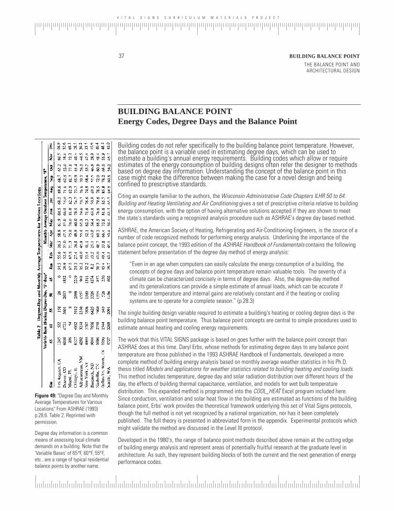
V I T A L S I G N S C U R R I C U L U M M A T E R I A L S P R O J E C T
BUILDING BALANCE POINT
THE BALANCE POINT ANDARCHITECTURAL DESIGN
37
BUILDING BALANCE POINTEnergy Codes, Degree Days and the Balance Point
Building codes do not refer specifically to the building balance point temperature. However,the balance point is a variable used in estimating degree days, which can be used toestimate a building's annual energy requirements. Building codes which allow or requireestimates of the energy consumption of building designs often refer the designer to methodsbased on degree day information. Understanding the concept of the balance point in thiscase might make the difference between making the case for a novel design and beingconfined to prescriptive standards.
Citing an example familiar to the authors, the Wisconsin Administrative Code Chapters ILHR 50 to 64:Building and Heating Ventilating and Air Conditioning gives a set of prescriptive criteria relative to buildingenergy consumption, with the option of having alternative solutions accepted if they are shown to meetthe state's standards using a recognized analysis procedure such as ASHRAE's degree day based method.
ASHRAE, the American Society of Heating, Refrigerating and Air-Conditioning Engineers, is the source of anumber of code recognized methods for performing energy analysis. Underlining the importance of thebalance point concept, the 1993 edition of the ASHRAE Handbook of Fundamentals contains the followingstatement before presentation of the degree day method of energy analysis:
“Even in an age when computers can easily calculate the energy consumption of a building, theconcepts of degree days and balance point temperature remain valuable tools. The severity of aclimate can be characterized concisely in terms of degree days. Also, the degree-day methodand its generalizations can provide a simple estimate of annual loads, which can be accurate ifthe indoor temperature and internal gains are relatively constant and if the heating or coolingsystems are to operate for a complete season.” (p.28.3)
The single building design variable required to estimate a building's heating or cooling degree days is thebuilding balance point temperature. Thus balance point concepts are central to simple procedures used toestimate annual heating and cooling energy requirements.
The work that this VITAL SIGNS package is based on goes further with the balance point concept thanASHRAE does at this time. Daryl Erbs, whose methods for estimating degree days to any balance pointtemperature are those published in the 1993 ASHRAE Handbook of Fundamentals, developed a morecomplete method of building energy analysis based on monthly average weather statistics in his Ph.D.thesis titled Models and applications for weather statistics related to building heating and cooling loads.This method includes temperature, degree day and solar radiation distribution over different hours of theday, the effects of building thermal capacitance, ventilation, and models for wet bulb temperaturedistribution. This expanded method is programmed into the COOL_HEAT Excel program included here.Since conduction, ventilation and solar heat flow in the building are estimated as functions of the buildingbalance point, Erbs' work provides the theoretical framework underlying this set of Vital Signs protocols,though the full method is not yet recognized by a national organization, nor has it been completelypublished. The full theory is presented in abbreviated form in the appendix. Experimental protocols whichmight validate the method are discussed in the Level III protocol.
Developed in the 1980's, the range of balance point methods described above remain at the cutting edgeof building energy analysis and represent areas of potentially fruitful research at the graduate level inarchitecture. As such, they represent building blocks of both the current and the next generation of energyperformance codes.
Figure 49: "Degree Day and MonthlyAverage Temperatures for VariousLocations" From ASHRAE (1993)p.28.6. Table 2. Reprinted withpermission.
Degree day information is a commonmeans of assessing local climatedemands on a building. Note that the'Variable Bases' of 65°F, 60°F, 55°F,etc.. are a range of typical residentialbalance points by another name.