building and ranking of geostatistical petroleum …
TRANSCRIPT
i
BUILDING AND RANKING OF GEOSTATISTICAL
PETROLEUM RESERVOIR MODELS
ODAI LOWESTEIN ADJEI

i
BUILDING AND RANKING OF GEOSTATISTICAL PETROLEUM RESERVOIR
MODELS
By
Odai Lowestein Adjei
RECOMMENDED:
APPROVED:
Prof. David Ogbe – Committee Chair
Prof. Ekwere Peters – Committee Member
Prof. Debasmita Misra – Committee Member
Chair, Department of Petroleum Engineering
Academic Provost
Date

i
BUILDING AND RANKING OF GEOSTATISTICAL
PETROLEUM RESERVOIR MODELS
A
THESIS
Presented to the Faculty
Of the African University of Science and Technology
in Partial Fulfillment of the Requirements
for the Degree of
MASTER OF SCIENCE
By
ODAI LOWESTEIN ADJEI
Abuja, Nigeria
December, 2010

iii
ABSTRACT
Techniques in Geostatistics are increasingly being used to generate reservoir
models and quantify uncertainty in reservoir properties. This is achieved through
the construction of multiple realizations to capture the physically significant
features in the reservoir. However, only a limited number of these realizations are
required for complex fluid flow simulation to predict reservoir future performance.
Therefore, there is the need to adequately rank and select a few of the realizations
for detailed flow simulation.
This thesis presents a methodology for building and ranking equiprobable
realizations of the reservoir by both static and dynamic measures. Sequential
Gaussian Simulation was used to build 30 realizations of the reservoir. The volume
of oil originally in place, which is a static measure, was applied in ranking the
realizations. Also, this study utilizes Geometric Average Permeability, Cumulative
Recovery and Average Breakthrough times from streamline simulation as the
dynamic measures to rank the realizations. A couple of realizations selected from
both static and dynamic measures were used to conduct a successful history match
of field water cut in a case study.

iv
DEDICATION
This research work is dedicated to;
The Holy Spirit - my constant comforter and help,
My Lovely Parents – Mr. Hayford Tawiah Odai and Veronica Awukubea Akuffo,
Diana Korkor Mensah – My dear friend,
My siblings – Cynthia, Leticia, Graham, Michael and Raymond
You keep my spirit alive!

v
ACKNOWLEGDEMENTS
This work would not have been possible if it had not been by the grace of the
Almighty God lavishly shed upon me. I thank God for the strength, inspiration,
guidance, and other provisions to carry out this research work successfully– to Him
alone be all the glory forever and ever.
Secondly, I express my gratitude to Professor David Ogbe for the immense
supervision of this work. Your fruitful effort and time spent on this thesis has gone a
long way to add quality to it – thank you.
Thirdly, my appreciation goes to Professor Ekwere Peters and Dr. Debasmita Misra
for the timely help they provided in editing the work. Also, I thank all petroleum
faculty members of AUST who have assisted by raising me up academically to be
able to carry out this work. The contributions you have made as far as this research
is concern are deeply recognized.
Fourthly, my acknowledgement goes to the Rocky Mountain Oilfield Testing Center
(RMOTC) for making available on their website part of the data used for this study.
Last but not least, I extend a hand of gratitude to my family, Diana Korkor Mensah,
and other colleagues of mine including Titus Ntow-Ofei and Azeb Demisi, for their
encouragement and concern. Your support no matter how small it is has been
significant to the success of this research work – thank you all.

vi
TABLE OF CONTENTS
Contents Page
SIGNATURE PAGE……………..………………….…………………………………………………………..I
TITLE PAGE…………………………………………………………………………….……………………….II
ABSTRACT ................................................................................................................................ III
DEDICATION ............................................................................................................................. IV
ACKNOWLEGDEMENTS .......................................................................................................... V
TABLE OF CONTENTS ............................................................................................................. VI
LIST OF FIGURES ..................................................................................................................... IX
LIST OF TABLES ........................................................................................................................ X
LIST OF APPENDICES ............................................................................................................. XI
CHAPTER ONE – INTRODUCTION ....................................................................................... 1
1.1 PROBLEM DEFINITION ............................................................................................................ 1
1.2 OBJECTIVES ................................................................................................................................... 2
1.3 SCOPE OF WORK ......................................................................................................................... 2
CHAPTER TWO – LITERATURE REVIEW .......................................................................... 4
2.1 INTRODUCTION .......................................................................................................................... 4
2.2 BUILDING OF GEOSTATISTICAL RESERVOIR MODELS ............................................. 4
2.2.1 Stochastic Simulation ............................................................................................................. 6
2.2.1.1 Sequential Gaussian Simulation (SGSIM) .............................................................. 6
2.3 RANKING OF GEOSTATISTICAL RESERVOIR MODELS .............................................. 8
2.3.1 Static Criteria ............................................................................................................................. 8
2.3.2 Dynamic Criteria ...................................................................................................................... 9
2.4 LITERATURE SUMMARY ...................................................................................................... 12
CHAPTER THREE – STUDY METHODOLOGY ................................................................. 13
3.1 INTRODUCTION ....................................................................................................................... 13
3.2 STUDY AREA .............................................................................................................................. 14

vii
3.3 DATA SUMMARY AND ANALYSIS ..................................................................................... 15
3.3.1 Analysis ..................................................................................................................................... 15
3.4 BUILDING OF RESERVOIR REALIZATIONS .................................................................. 22
3.5 RANKING OF RESERVOIR REALIZATIONS ................................................................ 26
3.5.1 Stock Tank Oil Originally in Place .................................................................................. 26
3.5.2 Geometric Average Permeability ................................................................................... 27
3.5.3 Connected Hydrocarbon Pore Volume ........................................................................ 28
3.5.4 Breakthrough times ............................................................................................................. 29
3.5.5 Cumulative Recovery .......................................................................................................... 31
3.6 FILTERING SELECTED REALIZATIONS BY RECOVERY AND WATER CUT ..... 31
3.7 CHAPTER SUMMARY .............................................................................................................. 32
CHAPTER FOUR –RESULTS AND DISCUSSION ............................................................... 33
4.1 BUILDING OF RESERVOIR MODELS ................................................................................ 33
4.2 RANKING OF THE RESERVOIR MODELS ....................................................................... 36
4.2.1 Static Ranking ......................................................................................................................... 36
4.2.2 Dynamic Ranking .................................................................................................................. 37
4.2.2.1 Geometric Average Permeability (kga) ................................................................ 37
4.2.2.2 Connected Hydrocarbon Pore Volume (CHPV) ............................................... 37
4.2.2.3 Average Breakthrough times (ABT) ..................................................................... 38
4.2.2.4 Cumulative Recovery (CR) ........................................................................................ 40
4.2.3 Relationship between Dynamic Ranking Criteria .................................................. 40
4.2.4 Application of Cumulative Recovery ............................................................................ 41
4.2.5 Application of Field Water Cut ........................................................................................ 44
4.3 HISTORY MATCHING.............................................................................................................. 45
4.4 CHAPTER SUMMARY .............................................................................................................. 48
CHAPTER FIVE – CONCLUSIONS AND RECOMMENDATIONS.................................... 49
5.1 SUMMARY AND CONCLUSIONS ......................................................................................... 49
5.2 RECOMMENDATIONS ............................................................................................................ 50

viii
REFERENCES ............................................................................................................................ 52
APPENDIX A: NOMENCLATURE .......................................................................................... 54
APPENDIX B: ADDITIONAL FIGURES AND TABLES FOR CHAPTER 3 ........................ 55
APPENDIX C: ADDITIONAL FIGURES AND TABLES FOR CHAPTER 4 ......................... 59
APPENDIX D: WORK FLOW FOR BUILDING AND RANKING GEOSTATISTICAL
RESERVOIR MODELS .............................................................................................................................. 65

ix
LIST OF FIGURES
Figure Page
3.1 Histogram and Variogram Analysis for Porosity…………..…………………………..17
3.2 Histogram and Variogram Analysis for Water Saturation………………………….18
3.3 Histogram and Variogram Analysis for Horizontal Permeability……..…………20
3.4 Histogram and Variogram Analysis for Vertical Permeability..........................21
3.5 Histogram and Variogram Analysis for Vertical Permeability……………………23
3.6 Cross – plot of kv versus kh………………………...……………………………………….......24
3.7 Schematic diagram for direct line waterflood pattern………………………….......30
4.1 Porosity Histogram Before and After SGSIM…………………………………………….35
4.2 Comparison between the Static and Dynamic Ranking Criteria…………………39
4.3 Comparison between the Dynamic Ranking Measures………………………………42
4.4 Cumulative Recovery after 15 years simulation versus percentiles from
other ranking measures…………………………………………………………………………..43
4.5 Field Water Cut History for selected realizations from both Static and
Dynamic criteria…………………………………………………………………………………....46
4.6 Water Cut History Match for selected realizations from both Static and
Dynamic Ranking Criteria……………………………………………………………………...47

x
LIST OF TABLES
TABLE Page
3.1 Tensleep Reservoir Data ………………………………………………………………………..15
3.2 Reservoir and Cell Dimensions ………………………………………………………………26
4.1 Brief summary of the Statistical Mean analyses ………………………………………34

xi
LIST OF APPENDICES
Page
APPENDIX A Nomenclature……………………………………………………………………54
APPENDIX B Additional Figures and Tables for Chapter 3……………………….55
Figure B1 Location Map of the Teapot Dome Oil Field………………………...55
Figure B2 Porosity Distribution before and after SGSIM……………………..56
Figure B3 Cross-plot Analysis of Petrophysical Properties………………….57
Table B1 Input Parameters for Variogram Computation and Modeling.58
APPENDIX C Additional Figures and Tables for Chapter 4……………………….59
Figure C1 Comparison of Cumulative Recoveries for selected percentile
Realizations from the Dynamic Criteria……………………………...59
Figure C2 Comparison of Cumulative Recoveries for selected percentile
Realizations from both Static and Dynamic Criteria…………….60
Figure C3 Analysis of selected realizations by WOR and Oil Rate
performance measures………………………………………………………61
Table C1 Values of each Criterion per Realization before
Ranking……………………………………………………………………………62
Table C2 Ranking Results for each Criterion…………………………………….63
APPENDIX D Work flow for building and Ranking Geostatistical Reservoir
Models……………………………………………………………………………...65

1
CHAPTER ONE – INTRODUCTION
1.1 PROBLEM DEFINITION
In Geostatistical reservoir characterization, it is a common practice to generate a
large number of realizations of the reservoir model to assess the uncertainty in
reservoir descriptions for performance predictions. However, only a limited fraction
of these models can be considered for comprehensive fluid flow simulations because
of the high computational costs. There is therefore the need to rank these
equiprobable reservoir models based on an appropriate performance criterion that
adequately reflects the interaction between reservoir heterogeneity and flow
mechanisms.
Most techniques used in ranking of realizations are based on static properties such
as highest pore volume, highest average permeability, and closest reproduction of
input statistics. The drawback of these simple techniques is that they do not account
for dynamic flow behavior which is very essential in predicting future reservoir
performance.
This thesis work seeks to build and rank equally probable representations of the
reservoir using petrophysical properties such as porosity, water saturation, and
permeability. The multiple reservoir descriptions are ranked using both static
(Stock tank oil originally in place) and dynamic (geometric average permeability,
connected hydrocarbon pore volume, average breakthrough times and cumulative
recovery) measures.

2
1.2 OBJECTIVES
The main purpose of reservoir characterization is to generate a more representative
geologic model of the reservoir properties. The objectives of this study are as
follows.
In building a static representation of what a reservoir is most likely to be it is
necessary to adequately capture the uncertainty associated with not knowing its
exact picture. In the effort of capturing the uncertainty, this study focuses on
generating multiple equiprobable realizations of the reservoir with each having
unique static and dynamic properties.
Only a few number of the realizations generated could be carried on for complex
flow simulation due to the computational cost. Usually ranking of the realizations to
select a limited number are done by static means which do not capture the dynamic
mechanisms essential to reservoir performance. Only few dynamic ranking
measures are currently in use. This research work seeks to define new dynamic
ranking criteria and compare them with existing criteria.
Another objective of this work is to evaluate the effectiveness of these new ranking
criteria using a field case study. How these criteria works for the actual field case
would confirm their efficacy.
The development of a workflow for building and ranking the realizations using
results of the case study is one of the objectives of this research work.
1.3 SCOPE OF WORK
An introduction to the work conducted is captured in Chapter one. Chapter two
gives a review of relevant literature, while the methodology for the generation and
ranking of equiprobable realizations of the reservoir is covered in Chapter 3.

3
Chapter 4 describes the results and observations. Finally, Chapter 5 presents
conclusions of the research and gives a set of recommendations.

4
CHAPTER TWO – LITERATURE REVIEW
2.1 INTRODUCTION
Development plans for oil and gas reservoirs requires huge investments. The
decision for making these investments is based on many factors including reservoir
performance predictions. To achieve sound reservoir performance predictions, a
reliable geological model is needed. However, there are a lot of challenges
encountered in the process of building reliable geological reservoir model. An
important challenge is the limited amount of information available to geoscientists.
Another challenge referred to as the non – uniqueness problem is that several
models can fit the same data and give different future forecasts (Al-Khalifa, 2004).
Moreover, stochastic modeling methods alone cannot predict accurately lithological
distribution.
To overcome these challenges, methods have been developed that integrate
different data such as well logs, 3D seismic and conceptual geologic models into a
comprehensive geologic model. Noticeably, the use of conceptual geologic models is
increasing in integrated geologic modeling, due to their role in adding geologic
knowledge. It is based on the geologist’s knowledge and results from the
interpretation of well data using geological rules. Unfortunately, integrated
geological models alone cannot solve the non – uniqueness problem (Al-Khalifa,
2004). For this reason, new techniques have been developed to rank geologic
models in selecting the most representative one to use in fluid flow simulations.
2.2 BUILDING OF GEOSTATISTICAL RESERVOIR MODELS
During Geostatistical reservoir characterization, it is a common practice to generate
a large number of realizations of the reservoir model to assess the uncertainty in

5
reservoir descriptions and performance predictions. Most commonly, these multiple
realizations account for spatial variations in petrophysical properties within the
reservoir and thus, represent a very limited aspect of uncertainty (Ates et al, 2003).
For reliable risk assessment, we need to generate realizations that capture a much
wider domain of uncertainty such as structural, stratigraphic, as well as
petrophysical variations.
In stochastic reservoir characterization, detailed field-scale geostatistical models of
reservoir heterogeneities are developed for reservoir management applications.
The aim of the stochastic approach in reservoir modeling is to quantify uncertainties
in reservoir performance for economic decisions. This new methodology results in
multiple, equi-probable models of the reservoir that are alternative images of
reservoir attributes in the inter-well space. The natures of the heterogeneities being
modeled, and the size and spatial distribution of the available data, determine the
number and size of the realizations needed to characterize uncertainties in the
reservoir description. In many cases, tens to hundreds of realizations are required
to characterize the uncertainties in the geologic model. The sources of the geologic
model uncertainties could be uncertainties in a number of factors: structural, facies
presence, facies spatial distribution and relationships, and petrophysical properties
for both static and dynamic attributes (Saad et al, 1996). The petrophysical
uncertainties generally tend to have a much lower impact on the reservoir
performance compared to factors affecting large-scale fluid movements (Ates et al,
2003). The size of geologic model grid cells is dictated by the scale of measurement
of the reservoir data available for modeling. However, the scale of measurement for
flow properties derived from cores and/or logs is relatively small, requiring small-
scale grid block representation in the geologic model (Saad et al, 1996). These
requirements result in realizations with a very large number of grid cells, and field-
scale models may contain several hundred thousand to several million cells. Even

6
with scale-up of reservoir properties, we are faced with hundreds of very large
reservoir models that must be used in flow simulation for uncertainty assessment.
2.2.1 Stochastic Simulation
Stochastic simulations provide a depiction and a measure of uncertainty of the
spatial variability of a phenomenon. This is done by generating multiple realizations
of the stochastic process modeling the spatial distribution under study. Several
simulation techniques have been developed, which can be classified into four
categories: sequential simulation, p-field simulation, object simulation and
optimization-based techniques. SGEMS the software employed for this thesis work
makes use of the sequential simulation category. Sequential simulation is a broad
class of algorithms which can be used to solve a very large spectrum of problems.
Under this category is the Sequential Gaussian Simulation (SGSIM) which was used
in generating the realizations for this study. Below is the algorithm for the SGSIM.
2.2.1.1 Sequential Gaussian Simulation (SGSIM)
Let Z(u) be a multivariate Gaussian random function with 0 mean, unit variance, and
a given covariance model. Realizations of Z, conditioned to data (n) can be generated
by following the algorithm below;
1. Define a random path visiting each node of the grid once
2. At each node u, the local conditional cumulative distribution function is Gaussian,
its mean is estimated by simple Kriging and its variance is equal to the simple
Kriging variance. The conditioning data consist of both neighboring original data (n)
and previously simulated values
3. Draw a value from that Gaussian ccdf and add the simulated value to the data set
4. Proceed to the next node in the path and repeat the two previous steps until all
nodes have been visited.
It can be shown that the resulting realizations will reproduce both the first and
second moments (covariance) of Z (Goovaerts et al, 1997). Note that the theory
7
requires the variance of each ccdf be estimated by the simple Kriging variance.
Algorithm SGSIM can account for non-stationary behaviors by using other types of
Kriging (see 2.2) to estimate the mean and variance of the Gaussian cdf. In that case
however, variogram reproduction is not theoretically ensured.
Histogram Transformation
The sequential Gaussian simulation algorithm as described above assumes that the
variable is Gaussian. If that is not the case, it is possible to transform the marginal
distribution of the variable into a Gaussian distribution and work on the
transformed variable. The transformation of variable Z(u) with cdf FZ into a
standard normal variable Y (u) with cumulative distribution function G is written:
( )))(()( 1 uZFGuY −= ……………………….. 2.1
This transformation does not ensure that Y is multivariate Gaussian, only its
histogram is. One should check that the multivariate (or at least bi-variate) Gaussian
hypothesis holds for Y before performing Gaussian simulation. If the hypothesis is
not appropriate, other algorithms that do not require Gaussianity, e.g. sequential
indicator simulation (SISIM) should be considered. The sequential Gaussian
simulation algorithm proceeds as follows:
1. Transform Z into a Gaussian variable according to Eq. (2.1)
2. Simulate Y as in Algorithm 1
3. “Back-transform” the simulated values y1, . . . , yN into z1, . . . ,zN:
( ))(1
iiyGFz −=
Ni ,...,1= ………………….2.2
In order to build a model of the reservoir, data from different sources such as
conceptual geologic model, well logs, well tests, seismic and production logs are
incorporated. There are multiple equi-probable geostatistical models possible with
each constrained to the given conditioning data (Yadav et al, 2006).

8
2.3 RANKING OF GEOSTATISTICAL RESERVOIR MODELS
With the wide-spread use of Geostatistics, it has now become a common practice to
generate a large number of realizations of the reservoir model to assess the
uncertainty in reservoir descriptions and performance predictions. However, only a
small fraction of these models can be considered for comprehensive flow
simulations because of the high computational costs (Ates et al, 2003). Randomly
choosing geological realizations will not accurately represent uncertainty; ranking is
therefore a superior method that selects cases that span production uncertainty
(Deutsch, 1996). The idea of ranking geostatistical realizations is not new (Ballin,
1992). The central goal of ranking is to exploit a relatively simple static measure to
accurately select geological realizations that correspond to targeted percentiles of
the production response (McLennan and Deutsch, 2005).
It is well known that a particular ranking measure must be highly correlated to
production response and that this correlation is achieved when calculation
procedure is tailored to the flow process (McLennan and Deutsch, 2005). This
framework has led to a variety of ranking methodologies and measures throughout
the petroleum industry. The measures can be grouped into two categories namely
static and dynamic criteria.
2.3.1 Static Criteria
This ranking category uses the static properties of the reservoir. Realizations could
be ranked based on highest pore volume, stock tank oil originally in place, highest
average porosity, closest reproduction of input statistics, and so on (Ates et al,
2003). Static ranking measures are straight forward and do not capture any
dynamic property of the reservoir.

9
2.3.2 Dynamic Criteria
Permeability which measures the reservoir’s ability to transmit fluid could be used
as a ranking criterion. Also, some type of permeability threshold connectivity can be
used to calculate connected pore volume and rank the realizations based on such
connectivity. Deutsch (2002b) reported that they can be easily calibrated to SAGD
production performance response with high correlation. Fenik et al (2009) showed
that ranking with connected hydrocarbon volume (CHV) can be correlated to SAGD
performance parameters. The connected hydrocarbon volume program was
developed to calculate the local connectivity using geoobjects within the window
based on the following equation:
∑∑= =
−=L
i
N
j
jjjSwui
LCHV
1 1
)1(**)(1
φ ………………………2.8
Where; CHV = connected hydrocarbon volume
L = number of realizations
N = number of grid cells
i(uj) = an indicator of connectivity (1 if connected, 0 otherwise)
φ j = reservoir porosity
Swj = Water Saturation
The drawback of these simple dynamic techniques (average permeability and CHV)
is that they do not account for dynamic flow behavior. A viable alternative is to rank
these multiple reservoir models based on an appropriate performance criterion that
adequately reflects the interaction between heterogeneity and the reservoir flow
mechanisms (Ates et al, 2003).
Dynamic flow simulation approximations employ quick flow-physics setups such as
random-walk, time-of-flight (TOF), and tracer or streamline setups. Dynamic
ranking measures and methodologies have received significant attention over the
past 14 years. Indeed it is tempting to use such fit-for-purpose measures for
10
ranking. Streamline simulation starts with the calculation of pressure distribution
and velocity field in the reservoir. The time of flight co-ordinate is used to decouple
saturation calculations. This reduces the multi-dimensional saturation equation into
a series of 1-D calculations along streamlines, hence the computational efficiency of
the streamline simulation (Ates et al, 2003). Saturation change is calculated along
the streamlines using either analytical or numerical methods. Time of flight which is
critical to streamline simulation is defined as the time required for a neutral particle
to travel from an injector to a producer. Production response at the wells is obtained
from multiphase transport equations along the streamlines in travel time
coordinates and summing up their contributions (Ates et al, 2003).
However there are a number of disadvantages. Most importantly, dynamic ranking
measures tend to exceedingly depend on the simplifying flow-physics
approximations rather than the underlying geological heterogeneity and
uncertainty (Gilman, 2005). The computational effort approaches that of a full flow
modeling (Saad et al, 1996). Moreover, several evolving production constraints such
as well placement and injection and production controls can be cumbersome to
incorporate into a dynamic methodology (Ates et al, 2003). Although dynamic
ranking certainly accounts for the production mechanism, these measures are not
simple and tend to undermine the geological uncertainty through its simplifying
assumptions (McLennan and Deutsch, 2005). Ates et al (2003) used the streamline
simulator to rank multi-million cell geostatistical reservoir descriptions based on
time-of-flight and to find the optimum level of vertical upscaling for finite-difference
simulation. They used the volumetric sweep efficiency as the main ranking criterion
for the multiple equiprobable realizations of a Middle Eastern carbonate reservoir
under a moderate to strong aquifer influx. The volumetric sweep is one of the
simplest performance measures that quantify the interactions between the
uncertainties in the static model with the dynamic flow conditions. The streamline

11
model is particularly well-suited for calculating the volumetric sweep based on the
time of flight connectivity (Ates et al, 2003). The following formulations were used.
∫ →=
u
dszyx
φτ ),,( ……………………………2.9
τ = time-of-flight; φ = porosity; u = velocity, s = distance
Once the time of flight is computed, the volumetric sweep at any time was computed
based on the time of flight distribution as follows;
∑∫ −=i
iisweptqtdtV )()()()( ψτθψτ …………………………..2.10
Where, θ is the Heaviside function and q(ψi) is the volumetric flow rate assigned to
the streamline ψi. Application of the methodology was the key to achieve a
satisfactory history match for the field example with minimal adjustments to the
reservoir model (Ates et al, 2003).
The overall recovery factor for waterflood secondary recovery technique is given
by;
sweptD VERF *=……………………..2.11
wi
wiwav
DS
SSE
−
−=1 ………………………..2.12
Where; Swav = average water saturation in the swept area
Swi = initial water saturation at the start of flood
Vswept = volumetric sweep efficiency;
ED = displacement efficiency
RF = overall recovery factor

12
2.4 LITERATURE SUMMARY
Building large number of reservoir static models to capture uncertainty is
fundamental in reservoir characterization. It is necessary to rank these models
based on an appropriate criteria that integrates reservoir heterogeneity and fluid
flow mechanisms to reduce the number of probable models for subsequent
performance predictions.
Most ranking measures are static and they lack the dynamics of the reservoir. Only a
few dynamic ranking measures like the volumetric sweep have been presented by
literature. This thesis work attempts to build distinct equiprobable reservoir
models, present new dynamic ranking measures, integrate the results from these
dynamic measures to select a reduced number of models and compare the results to
that of the static measure. Also, the performance criteria – field water cut, is used as
a measure of comparison between the static and dynamic ranking criteria.

13
CHAPTER THREE – STUDY METHODOLOGY
3.1 INTRODUCTION
Most often than not, petroleum reservoirs are located several depths below the
earth surface. This makes it difficult to accurately characterize the reservoir and
correctly generate a true representation of it since its entirety is invisible. Therefore,
it is a normal practice in reservoir modeling to build a large number of equally
potential reservoir realizations. These equiprobable multiple-cell realizations are
built in order to fairly capture the uncertainty associated with subsurface reservoir
studies. Basically, they provide static possible outlooks of the reservoir.
Flow simulation studies need to be carried out to gain a substantial understanding
of the reservoir dynamics and its relationship with the static model. From this
exercise, future predictions of reservoir performance could be made which would in
turn adequately inform critical economic and operational decision making. Detailed
flow simulation of a petroleum reservoir is computationally intensive and therefore
very expensive. Hence, it is necessary to scale-up and reduce the large number of
equiprobable realizations of the petroleum reservoir built at the early stages. This
requires an appropriate ranking criterion to short-list this set of multiple reservoir
representations.
Many criteria have been used in ranking reservoir realizations. Average porosity
(AP), hydrocarbon pore volume (HPV), and Stock Tank Oil Originally in Place
(STOOIP) are some of the static measures that have been used in ranking
realizations. To represent the reservoir dynamics in the ranking process, other
measures like Connected Hydrocarbon Pore Volume (CHPV) and Volumetric sweep
efficiency have been used. In this study, STOOIP, Geometric Average Permeability
(kga), CHPV, Breakthrough time and Cumulative Recovery are used as ranking
criteria.
14
3.2 STUDY AREA
Teapot Dome field, also known as Naval Petroleum Reserve #3 (NPR-3) is located in
the southwest portion of the Powder River Basin, 35 miles north of Casper,
Wyoming in the Natrona County (See Appendix B). The reserve is a Government-
owned oil field of 9,481 acres and was established in 1915 by executive order from
President Wilson and became famous during the 1920’s scandals of the Harding
administration. The field is operated by the Department of Energy (DOE) through its
Rocky Mountain Oilfield Testing Center (RMOTC).
Tensleep reservoir which is of a shallow marine to terrigenous eolian origin is one
of the nine oil reservoirs located in the Teapot Dome field. It is chiefly made of fine
to very fine grained cross-bedded sandstone with quartz and carbonate
cementation. The Tensleep reservoir has an aerial extent of about 310 acres located
at an average depth of about 5500ft. The original oil in place is estimated to be
approximately 4.5 MMSTB (Garcia, 2005).
Oil in the Tensleep reservoir is dark-brown, sour crude with an intermediate wax-
bearing base. The crude oil is highly undersaturated. Oil gravity ranges from 15 0API
to near 25 0API whereas the viscosity varies from 20 cp to more than 100cp. Initial
formation volume factor is estimated to be 1.312 RB/STB. The Tensleep formation
water is relatively fresh with only 4,000ppm total solids.
Data used for this research was obtained from the Tensleep reservoir. All analyses
were conducted based on the available data from Papers and the Rocky Mountain
Oilfield Testing Center (RMOTC) website. Several wells have been drilled into the
Tensleep reservoir but data from 22 wells were used in this work.
15
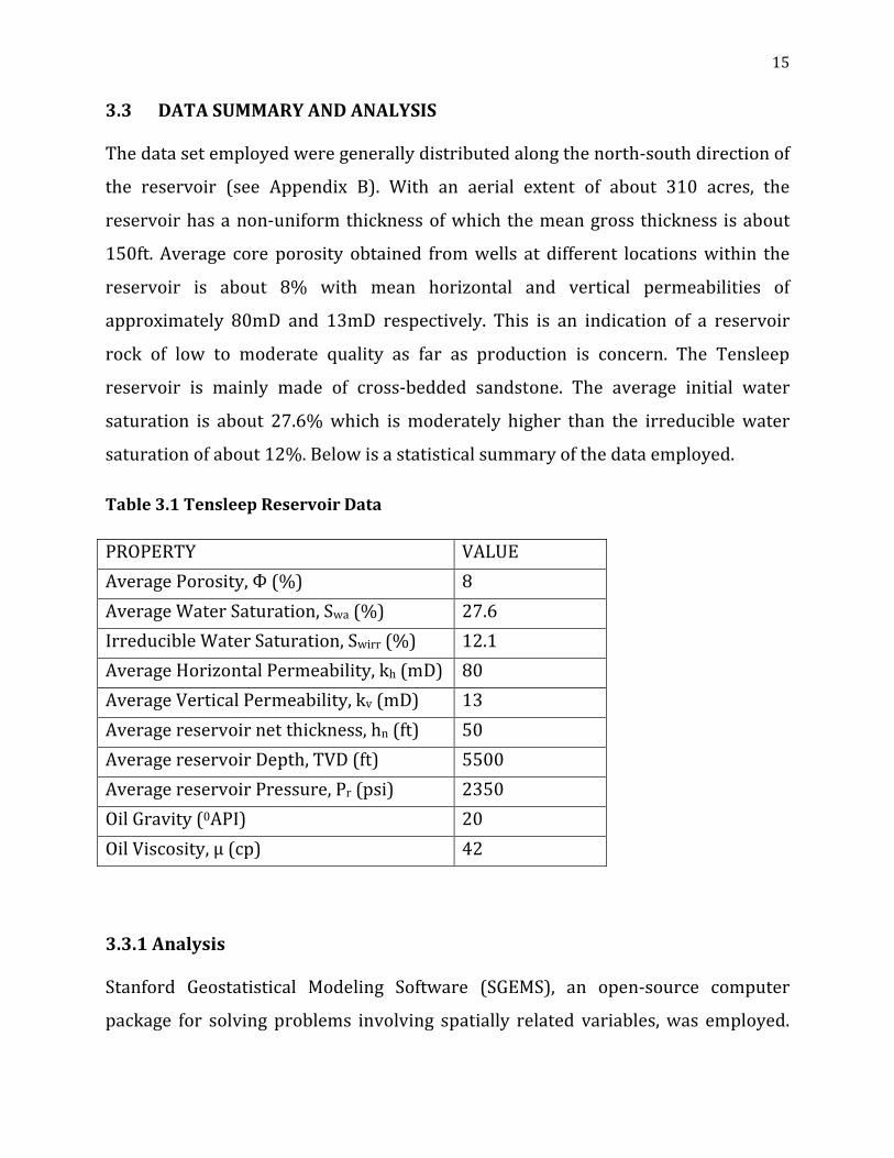
3.3 DATA SUMMARY AND ANALYSIS
The data set employed were generally distributed along the north-south direction of
the reservoir (see Appendix B). With an aerial extent of about 310 acres, the
reservoir has a non-uniform thickness of which the mean gross thickness is about
150ft. Average core porosity obtained from wells at different locations within the
reservoir is about 8% with mean horizontal and vertical permeabilities of
approximately 80mD and 13mD respectively. This is an indication of a reservoir
rock of low to moderate quality as far as production is concern. The Tensleep
reservoir is mainly made of cross-bedded sandstone. The average initial water
saturation is about 27.6% which is moderately higher than the irreducible water
saturation of about 12%. Below is a statistical summary of the data employed.
Table 3.1 Tensleep Reservoir Data
PROPERTY VALUE
Average Porosity, Ф (%) 8
Average Water Saturation, Swa (%) 27.6
Irreducible Water Saturation, Swirr (%) 12.1
Average Horizontal Permeability, kh (mD) 80
Average Vertical Permeability, kv (mD) 13
Average reservoir net thickness, hn (ft) 50
Average reservoir Depth, TVD (ft) 5500
Average reservoir Pressure, Pr (psi) 2350
Oil Gravity (0API) 20
Oil Viscosity, μ (cp) 42
3.3.1 Analysis
Stanford Geostatistical Modeling Software (SGEMS), an open-source computer
package for solving problems involving spatially related variables, was employed.

16
Each reservoir property data set was assessed using histograms, cross-plots, and
variogram analyses. Input parameters for the variogram computation and modeling
can be seen in Appendix B – Table B1. Generally, anisotropic variograms were
considered to adequately capture the spatial correlation between data points. The
properties evaluated are porosity, water saturation, horizontal and vertical
permeabilities, and reservoir thickness.
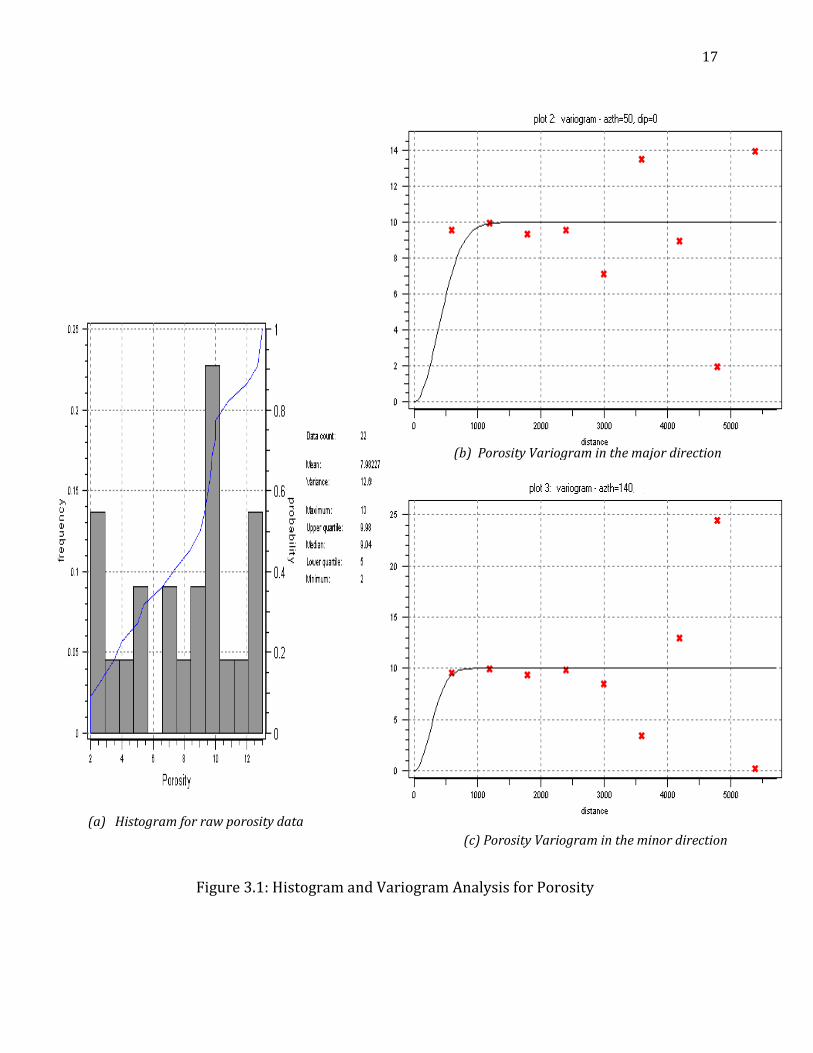
a) Porosity
The minimum and maximum raw porosity values are 2% and 13% respectively.
From the histogram plot of the porosity data a unimodal distribution was observed
(Figure 3.1a). The most occurring or likely porosity values are between 9% and
10.5%. The mean porosity value is 8% while the standard deviation is 3.5%.
Variogram analysis which measures the degree of spatial variation in the data set
was then conducted on the porosity data set to subsequently aid in the generation of
equiprobable realizations. Gaussian model was used to fit the data set by visual
inspection. The spatial variation in the porosity data points were adequately
captured in two variogram directions. Figures 3.1b and 3.1c respectively show the
major and minor directional variograms employed.
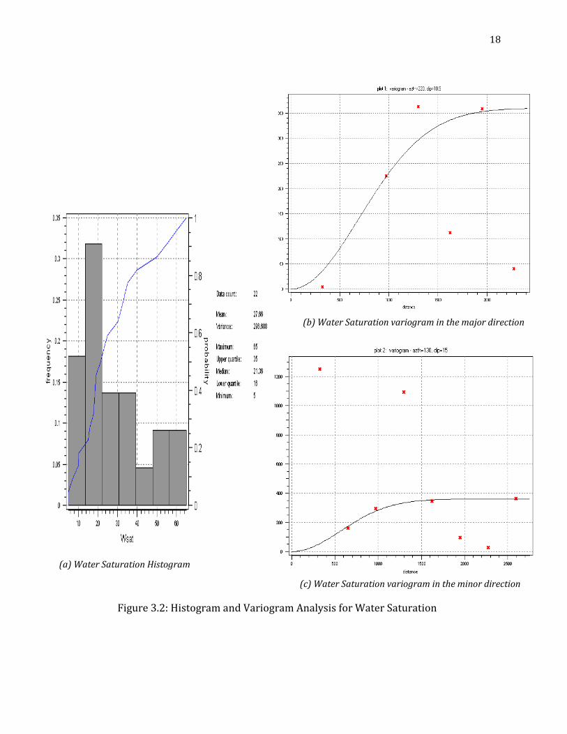
b) Water Saturation
Water saturation distribution at initial reservoir conditions was considered in this
study because of its application in the STOOIP ranking criterion. The histogram of
water saturation is shown in Figure 3.2a. Notice that 5% and 65% are the respective
minimum and maximum water saturations. A unimodal distribution was observed
from the histogram plot of the water saturation data. The range of 13 – 22%
contains the most occurring or likely water saturation values. The average water
saturation is 27.6% while the standard deviation is 17.2%.
17
(a) Histogram for raw porosity data
(b) Porosity Variogram in the major direction
(c) Porosity Variogram in the minor direction
Figure 3.1: Histogram and Variogram Analysis for Porosity
18
(b) Water Saturation variogram in the major direction
(c) Water Saturation variogram in the minor direction
(a) Water Saturation Histogram
Figure 3.2: Histogram and Variogram Analysis for Water Saturation
19
By visual inspection, Gaussian variogram model was used to fit the water saturation
data set from the variogram analysis conducted. The major and minor directional
variograms used in adequately capturing the spatial correlation in the water
saturation data set are shown in Figures 3.2b and 3.2c.
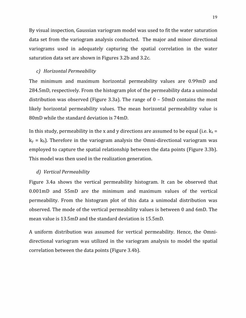
c) Horizontal Permeability
The minimum and maximum horizontal permeability values are 0.99mD and
284.5mD, respectively. From the histogram plot of the permeability data a unimodal
distribution was observed (Figure 3.3a). The range of 0 – 50mD contains the most
likely horizontal permeability values. The mean horizontal permeability value is
80mD while the standard deviation is 74mD.
In this study, permeability in the x and y directions are assumed to be equal (i.e. kx =
ky = kh). Therefore in the variogram analysis the Omni-directional variogram was
employed to capture the spatial relationship between the data points (Figure 3.3b).
This model was then used in the realization generation.
d) Vertical Permeability
Figure 3.4a shows the vertical permeability histogram. It can be observed that
0.001mD and 55mD are the minimum and maximum values of the vertical
permeability. From the histogram plot of this data a unimodal distribution was
observed. The mode of the vertical permeability values is between 0 and 6mD. The
mean value is 13.5mD and the standard deviation is 15.5mD.
A uniform distribution was assumed for vertical permeability. Hence, the Omni-
directional variogram was utilized in the variogram analysis to model the spatial
correlation between the data points (Figure 3.4b).

20
(a) Horizontal Permeability Histogram
Figure 3.3: Histogram and Variogram Analysis for Horizontal Permeability
(b) Omni-directional variogram for Horizontal Permeability

21
(a) Vertical Permeability Histogram
Figure 3.4: Histogram and Variogram Analysis for Vertical Permeability
(b) Omni-directional variogram for Vertical Permeability

22
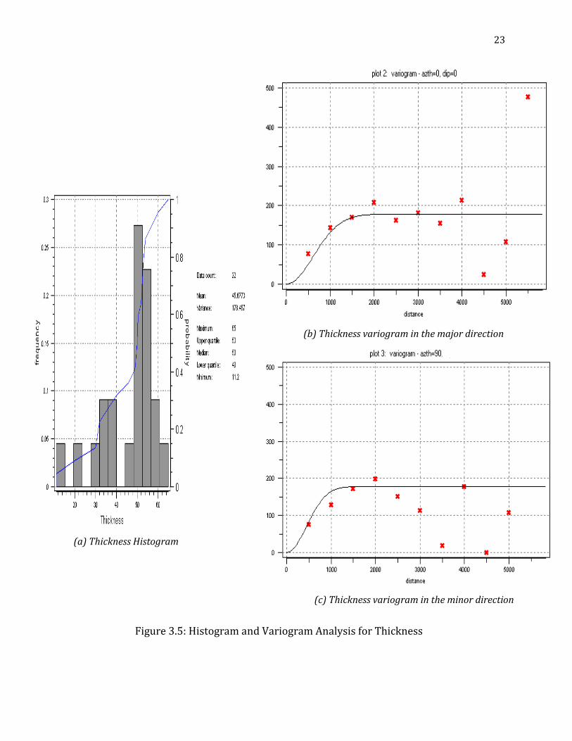
e) Thickness
The non-uniform net thickness distribution is characterized by minimum and
maximum values of 11.2ft and 65ft, respectively. From the histogram plot of the
thickness data a unimodal distribution was observed (Figure 3.5a). The most likely
thickness values fall between 48ft and 53ft. The mean thickness value is 46ft whiles
the standard deviation is 13ft.
Gaussian model was used to fit the thickness data from the variogram analysis.
Figures 3.5b and 3.5c respectively show the major and minor directions in which the
variogram analysis was conducted.
f) Cross – Plot Analysis
Cross-plots of vertical permeability versus horizontal permeability, permeability
versus porosity, and water saturation versus porosity from the various wells were
analyzed. From the analyses, only the vertical versus horizontal permeability
showed a fair correlation (Figure 3.6). The others showed weak correlation (see
Appendix B)
3.4 BUILDING OF RESERVOIR REALIZATIONS
Simulation was employed in the statistical estimation of the reservoir properties
over the entire volume of the Tensleep reservoir model. Stochastic simulation
method was used as opposed to kriging due to the following reasons;
� Multiple equiprobable realizations of the reservoir is possible
� Honor well data, histogram and Variogram used in quality control of the data.
� Allows flow simulations to be done and
� Makes uncertainty calculations possible.
23
(c) Thickness variogram in the minor direction
(b) Thickness variogram in the major direction
(a) Thickness Histogram
Figure 3.5: Histogram and Variogram Analysis for Thickness

24
y = 0.019x1.377
R² = 0.535
0.00
0.00
0.01
0.10
1.00
10.00
1.00 10.00 100.00 1000.00
Ve
rtic
al
Pe
rme
ab
ilit
y, k
v(m
D)
Horizontal Permeability, kh (mD)
Cross-Plot of kv Versus kh
Figure 3.6: Cross-plot of kv against kh

25
Sequential Gaussian Simulation (SGSIM) was used to generate 30 realizations each
for porosity, water saturation, horizontal permeability, vertical permeability and
thickness. The parameters obtained from the variogram analysis were used in this
exercise. For each property a maximum conditioning data of 12 was used with a
seed value of 14071789.
The SGSIM employed the mean and variance of simple kriging in which the trend
component is assumed to be constant and mean is known. The Kriged surface was
smoother than the true surface. SGSIM assumes that the variable is Gaussian. If that
is not the case, it is possible to transform the marginal distribution of the variable
into a Gaussian distribution and work on the transformed variable. Below is the
summary of the algorithm that was followed in generating the realizations for each
of the reservoir property.
1. Transform Z into a Gaussian variable according to Eq. (2.1)
2. Simulate Y
3. “Back-transform” the simulated values y1, . . . , yN into z1, . . . ,zN:
( ))(1
iiyGFz −=
Ni ,...,1= ………………….3.1
Data obtained after generating realizations for each reservoir property were then
merged for each cell using Microsoft Excel. In all a total of 32,900 cells were
generated over the entire reservoir volume for each realization. Each cell is
characterized by an average porosity, water saturation, horizontal and vertical
permeabilities, and thickness values which together depict a fair representation of
reservoir heterogeneity. Table 3.2 shows a summary of the reservoir dimensions
and grid data used.

26
Table 3.2 Reservoir and Cell dimensions
Reservoir Dimensions (in feet)
Length 6101
Width 2280
Gross Thickness 150
Net Thickness 50
Average Reservoir Depth 5500
Cell Dimensions (in feet)
Length 64
Width 64
Thickness 15
Number of Cells in the X-direction 35
Number of Cells in the Y-direction 94
Number of Cells in the Z-direction 10
Total Number of cells 32,900
3.5 RANKING OF RESERVOIR REALIZATIONS
The 30 realizations generated above using SGEMS need to be reduced to a small
number in order to cut down the cost of comprehensive flow simulations. In this
regard, the reservoir representations built were ranked based on STOOIP, kga, CHPV,
Breakthrough times and Cumulative Recovery. The STOOIP measure represents the
static ranking criteria whereas the kga, CHPV and Average Breakthrough Time
measures make up the dynamic criteria.
3.5.1 Stock Tank Oil Originally in Place
The total volume of oil initially in place in the reservoir was used as a ranking
criterion. OOIP for each cell was determined from equation 3.2.
oi
wiccc
B
ShASTOOIP c
)1(****7758 −=
ϕ………………………………………………….3.2

27
Where Boi = Initial Oil Formation Volume Factor (RB/STB); Ac = Area of cell;
hc = cell thickness; φc = cell porosity; Swic = cell initial water
saturation
Again, the total STOOIP for each realization was calculated from equation 3.3.
( )∑=
−=n
ccwi
oi
R ShAB
STOOIP1
)1(***7758
ϕ …………………………………………..3.3
Where n = total number of cells per realization (i.e. 32900 cells).
The 30 realizations were then ranked from the highest to the lowest STOOIP values.
In this order the 10th, 50th and 90th percentile realizations were obtained based on
the STOOIP values and compared with the same from other ranking criteria. In the
realization selection process, the 10th, 50th, and 90th percentile values were used in
order to have a fair representation of uncertainty in terms of low, medium and high
values of STOOIP.
3.5.2 Geometric Average Permeability
Permeability which measures the reservoirs ability to transmit fluids is a dynamic
property. Using the horizontal and vertical permeability values, a geometric average
permeability was calculated for each grid cell from equation 3.4. An average of the
kga for each realization was then used in the ranking process. This measure is a
geometric average and does not take into consideration permeability anisotropy in
the reservoir. However, its application in this work adds to the selected number of
probable representations of the reservoir.
( )vhga kkk *= …………………………………..3.4
Where kga = Geometric Average Permeability
kh = horizontal permeability
kv = vertical permeability.

28
Furthermore, the realizations were ranked from the highest geometric average
permeability to the lowest. To capture uncertainty, the realizations corresponding
to P10, P50 and P90 of the average permeability values were selected and compared
with the same from other ranking criteria.
3.5.3 Connected Hydrocarbon Pore Volume
The connected hydrocarbon pore volume is a ranking measure which seeks to inter-
relate reservoir static and dynamic properties. It is a measure of the reservoir pore
volume that contains connected hydrocarbon.
This ranking criterion employs the use of cut-offs for the basic reservoir properties.
Since permeability (k) is a dynamic reservoir property it is the key parameter used
in defining connectivity even though cut-offs for oil saturation and porosity are also
used. For example if the value of the permeability cut-off is 5mD then any cell whose
k value falls below this will not be counted in the calculation and will be considered
as non-connected cell. In this criterion the geometric average permeability defined
by equation 3.4 was used.
The cut-off values employed in this work for the geometric average permeability,
porosity and water saturation are 10mD (due to high oil viscosity), 4% (i.e. the
lower mean porosity quartile) and 72% (i.e. at irreducible oil saturation)
respectively. Equation 3.5 is used in the calculation of the CHPV for each realization.
( )
−= ∑
=
n
ccjwiR uiShACHPV
1
)(*)1(****7758 ϕ ………………….………3.5
Where i (uj) = connectivity indicator (1 if connected and 0 if otherwise). Note; the
terms A, h, φ and Swi are defined in equation 3.2
Again, the 30 realizations were then ranked from the highest to the lowest value of
CHPV. Realizations corresponding to P10, P50 and P90 of CHPV were obtained in
the same manner as before and compared with other ranking criteria.

29
3.5.4 Breakthrough times
A simple direct line flooding which involves five producers and five injectors located
respectively at the east and west side of the reservoir models was employed.
Arrangement of wells was done along the north-south direction of the reservoir. The
distance between wells of the same type is about 1152ft and that between lines of
producers and injectors is about 2112ft. Figure 3.7 shows the schematic diagram of
the water flood pattern used in this study.
A 3-dimensional streamline simulation run was carried out for 10 years using S3D
software (Datta-Gupta and King, 2007) and the breakthrough time for each well in a
realization was recorded. This breakthrough time was obtained from the time of
flight formulation. Time of flight is the total travel time of the injected water tracer
from an injector to a producer. This is given by equation 3.6 where the integration is
done over the distance from the injector to the producer.
∫ →=
u
dszyx
φτ ),,( …………………………………...3.6
Where: τ = time-of-flight; φ = porosity; u = velocity, s = distance
The average of these breakthrough times was obtained and assigned per realization.
The realizations were then ranked in the order of highest average breakthrough
times (ABT), after which the P10, P50 and P90 realizations were selected. The
selected realizations were then compared with the same from other ranking criteria.

30
Injector 1
Injector 2
Injector 3
Injector 5
Injector 4
Producer 1
Producer 2
Producer 3
Producer 4
Producer 5
Figure 3.7 Schematic diagram for direct line waterflood pattern

31
3.5.5 Cumulative Recovery
The simple direct line waterflood pattern as employed in the case of breakthrough
times was used and the cumulative recoveries for each realization after a 10 – year
simulation, were recorded. Cumulative recovery was obtained as a fraction of the
original oil initially in place that has been recovered over the period of 10 years.
N
NR
p
cum = ………………………………………3.7
Where; Rcum = Cumulative recovery
NP = Cumulative oil production over the total number of years (10 years)
N = Original oil initially in place.
Subsequently, these cumulative recovery values were also used to rank the 30
realizations from the highest to the lowest. Realizations corresponding to P10, P50
and P90 were obtained in the same manner as before and compared with other
ranking criteria.
3.6 FILTERING SELECTED REALIZATIONS BY RECOVERY AND WATER CUT
3–Dimensional streamline simulation was carried out for an additional 5 years
making a total of 15 years and the cumulative recovery was recorded. This was done
for each of the selected realizations corresponding to the percentiles from each
ranking criteria (with the exception of those from the Cumulative recovery criteria).
The cumulative recoveries from the selected realizations were compared for each
ranking criteria, among the dynamic criteria and between the static and dynamic
criteria. By using the cumulative recovery as a filter, three realizations were selected
from the dynamic criteria corresponding to P10, P50 and P90. This was done by
comparing and selecting the realization with the highest cumulative recovery for
32
each percentile of the kga, CHPV and ABT. Also, the three realizations picked from
the STOOIP criteria were used to represent the static selected realizations.
Subsequently, the field water cut histories obtained from each of the selected
percentile realizations were compared between those of the static and dynamic
criteria. This was done to show the criteria whose realizations have a better field
performance and also to select those realizations whose water cut histories are
closest to that of the actual field case. Field Oil rates associated with the selected
realizations were also compared.
3.7 CHAPTER SUMMARY
Sequential Gaussian Simulation was employed to generate 30 equiprobable
realizations of the reservoir. These realizations were then ranked by both static and
dynamic criteria. A total of 12 realizations were selected out of the 30, comprising
four sets of three realizations corresponding to P10, P50 and P90 from STOOIP, kga,
CHPV and breakthrough times. The cumulative recovery after 15 years was used as
a filter to reduce the dynamic set of 9 realizations to 3. Field water cut histories for
the selected realizations were then compared.
The following chapter presents discussions of the results obtained from the work
done.

33
CHAPTER FOUR –RESULTS AND DISCUSSION
The results obtained from this research work are presented in this chapter. Analysis
of the results is discussed and pertinent observations derived from the results are
also included in this presentation.
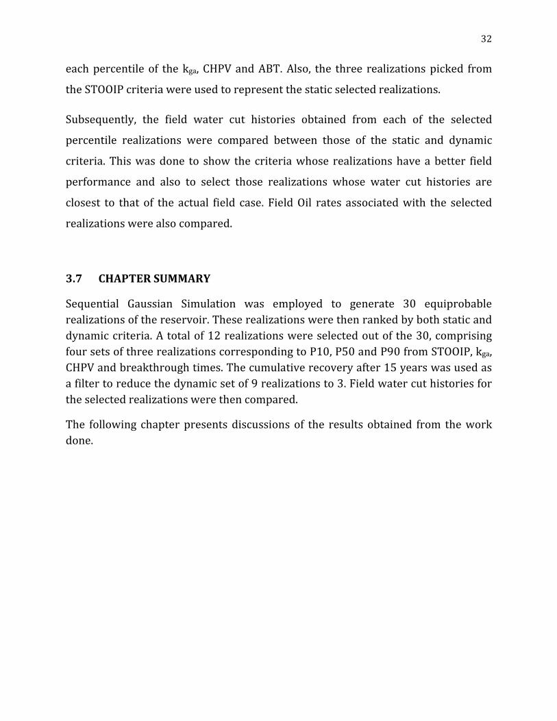
4.1 BUILDING OF RESERVOIR MODELS
In all 30 static equiprobable descriptions of the reservoir were generated with
SGEMS. Table 4.1 shows the results of the statistical means obtained from the
realizations generated for porosity, water saturation, horizontal permeability,
vertical permeability, and net thickness.
Generally, the mean values after simulation of the petrophysical properties are
slightly smaller than those of the raw data. This observation may be attributed to
the variogram parameters employed for each property. That notwithstanding, the
mean before and after are fairly close for all the properties used in building the
realizations. The implication of this observation is that, statistically the realizations
generated are of good quality. This degree of quality is depicted in Figure 4.1a which
shows the porosity histogram for realization 7. The mode and mean together with
other statistical parameters of this realization are quite similar to those of the raw
data shown in Figure 4.1b.

34
Table 4.1 Brief summary of the Statistical Mean analyses before and after building
the realizations
PROPERTY BEFORE SGSIM AFTER SGSIM
Real.
Number
Porosity (%) Mean 9.72
Minimum mean 3.5 15
Mean (for all realizations) 3.9
Maximum Mean 4.3 13
Water Saturation
(%) Mean 33.05
Minimum mean 18.5 15
Mean (for all realizations) 22.5
Maximum Mean 24.9 22
Horizontal
Permeability
(mD)
Mean 83.27
Minimum mean 42.3 14
Mean (for all realizations) 49.2
Maximum Mean 53.0 21
Vertical
Permeability
(mD)
Mean 10.71
Minimum mean 4.7 15
Mean (for all realizations) 5.7
Maximum Mean 5.6 1
Thickness (ft) Mean 10.29
Minimum mean 50.99 15
Mean (for all realizations) 60.27
Maximum Mean 58.92 1
Also the reasonable variation in the maximum and minimum average values (Table
4.1) suggests that the extreme high and low cases of what the static reservoir model
could be was fairly represented.
Realizations 16, 21, 4, 15 and 28 are the realizations whose mean porosity, water
saturation, vertical and horizontal permeability, and thickness values are closest to
that of the raw data used.
Realization 6 which has the highest mean value for porosity eventually had the
highest STOOIP (5.8 MMSTB) and CHPV (6.4 MMRB) as would normally be expected.
Conversely, realization 9 with the lowest porosity mean value emerged as the
realization with the lowest STOOIP (3.6 MMSTB) and CHPV (3.7 MMRB).
35
(a) Porosity Histogram for realization 7 (b) Porosity Histogram before SGSIM
Figure 4.1 – Porosity Histogram Before and After SGSIM
36
4.2 RANKING OF THE RESERVOIR MODELS
The 30 realizations were ranked using both static and dynamic measures. The static
measures do not consider fluid flow mechanism in the reservoir. The main reservoir
parameters used in this measure are porosity, water saturation, oil formation
volume factor, net thickness and area. This measure is mainly the stock tank oil
originally in place. However, the dynamic ranking criteria consider the reservoir
permeability, fluid saturations and mobility, and pressure among others. These
measures are Geometric Average Permeability (kga), connected hydrocarbon pore
volume (CHPV), average breakthrough times (ABT) and cumulative recovery (CR).
4.2.1 Static Ranking
The highest and lowest STOOIP values obtained are 5.8 MMSTB and 3.6 MMSTB,
respectively. This again is a fair reflection of the extreme high and low cases of
uncertainty captured in the realizations. The wide variation in the realizations
generated gives a broader range within which the most probable representation of
the reservoir would fall. It is observed that the estimated STOOIP (4.5 MMSTB) for
the Tensleep reservoir falls within the above range.
Realization 6 came out with the highest STOOIP. This could be inferred from its
highest average porosity value. Realizations 1 and 13 showed medium values of the
static ranking measure, whereas realization 9 came out with the minimum STOOIP
partly due to its lowest mean porosity. The static ranking results could be seen in
Appendix C (Table C2).
Using percentile evaluation, it is observed that the P10, P50 and P90 realizations are
number 18, 13 and 23, respectively. Primarily, this selection process seeks to
represent the low, medium and high cases of uncertainty in the reservoir
descriptions generated. Also, it was used to reduce the large number of models into
a limited quantity (three) for subsequent fluid flow simulation.

37
4.2.2 Dynamic Ranking
Geometric average permeability, connected hydrocarbon pore volume, average
breakthrough time and cumulative recovery were the main yardsticks used in this
method of ranking.
The kga and CHPV considered the permeability and fluid properties of the reservoir
at initial conditions. Pressure and time factors were not taken into account in these
two ranking criteria and are therefore partially dynamic. Their dynamic
classification is due to the permeability and fluid saturation considered.
On the other hand, the average breakthrough time and cumulative recovery are
dynamic ranking measures that consider pressure and time components among
other relevant factors. They are therefore the comprehensive dynamic measures
used in this study.
4.2.2.1 Geometric Average Permeability (kga)
The highest and lowest average effective permeabilities obtained were 39.8 mD and
17.8 mD for models 5 and 11, respectively. As shown in Figure 4.2a, this criterion
had little correlation with the STOOIP criteria due to the lack of direct relationship
between the static and dynamic properties of the reservoir. The implication of this is
that, both cannot be used alternatively to rank reservoir models. The P10, P50 and
P90 selections based on kga corresponded to realizations 25, 30 and 9.
4.2.2.2 Connected Hydrocarbon Pore Volume (CHPV)
The CHPV compared very well with the STOOIP ranking measure. This may be due
to its partial relationship with the static properties of the reservoir (i.e. both
measures use porosity and other reservoir parameters like thickness and area).
Figure 4.2b shows a cross-plot of CHPV versus STOOIP. Even though the correlation
was very good, not all CHPV ranks matched with the static (STOOIP) ranks. For
example, realization 24, which was ranked 23rd in the CHPV, was ranked 18th in the
38
static STOOIP criteria. Again, realization 5 ranked 15th by CHPV was ranked 25th by
the STOOIP measure. This observation of indirect correlation implies that a
realization with a high STOOIP rank would not necessarily have a high CHPV rank
and vice versa due to the dynamic component of the CHPV measure.
Not all the pore volumes containing hydrocarbons in the reservoir are connected.
This can be inferred from the lower CHPV values compared with the hydrocarbon
pore volume (HPV), signifying that reservoir pore volume is not perfectly related to
its connectivity.
Again, realizations 6 (6.4 MMRB) and 9 (3.7 MMRB) produced the highest and
lowest CHPV, respectively. From this CHPV criterion, realizations 22, 26 and 10
correspond to P10, P50 and P90.
4.2.2.3 Average Breakthrough times (ABT)
This dynamic measure is relatively new in the ranking of equiprobable reservoir
realizations. In this study, the average breakthrough times obtained for the
realizations range between 1 and 5 years.
Realizations 4 and 2 showed the earliest and latest average breakthrough times.
Based on the percentiles, models 6, 10 and 7 corresponding to P10, P50 and P90
were selected for further analysis.
There is basically no clear correlation between this measure and the static measure
as would normally be expected (Figure 4.2c). This observation emphasizes that
both measures have no direct relationship and therefore static and dynamic ranking
measures cannot be used alternatively. However, employing both criteria in ranking
reservoir models gives a wider window within which the most probable reservoir
representation would fall.

39
15
20
25
30
35
40
45
3.6 4.1 4.6 5.1 5.6 6.1
kg
a(m
D)
STOOIP, MMSTB
kga Versus STOOIP
y = 1.302x - 1.303R² = 0.841
3.5
4.0
4.5
5.0
5.5
6.0
6.5
7.0
3.5 4.5 5.5 6.5
CH
PV
, MM
RB
STOOIP, MMSTB
CHPV Versus STOOIP
1.5
2.0
2.5
3.0
3.5
4.0
4.5
4 5 6
AB
T (
Ye
ars
)
STOOIP (MMSTB)
ABT Versus STOOIP
0.35
0.37
0.39
0.41
0.43
0.45
0.47
0.49
0.51
0.53
3.5 4.0 4.5 5.0 5.5 6.0
Cu
mu
lati
ve
Re
cov
ery
STOOIP, MMSTB
CR Versus STOOIP
(d) Cross-plot of Cumulative Recovery versus
STOOIP for all realizations
(a) Cross-plot of kga versus STOOIP for all realizations (b) Cross-plot of CHPV versus STOOIP for all realizations
(c) Cross-plot of Average Breakthrough Times
versus STOOIP for all realizations
Figure 4.2 – Comparison between the Static and Dynamic Ranking Criteria

40
4.2.2.4 Cumulative Recovery (CR)
Cumulative recovery is also a dynamic ranking criterion. Over the 10-year
simulation run of a line drive waterflood, the highest cumulative recovery recorded
from all the realizations is about half of the original oil in place. Realizations 8 and 6
are the realizations with the highest (51%) and lowest (40%) cumulative
recoveries, respectively (See Appendix C – Table C2).
Figure 4.2d shows a poor correlation between the cumulative recovery and the
static measure. This can be explained by the lack of clear or direct relationship
between cumulative recovery and original oil initially in place and hence cannot be
used to substitute each other in the ranking of reservoir models.
However, realization 6 with the highest STOOIP produced the lowest recovery
whereas model 9 which has the lowest STOOIP has a high recovery. The implication
of this observation is that high STOOIP value does not guarantee high cumulative
recovery.
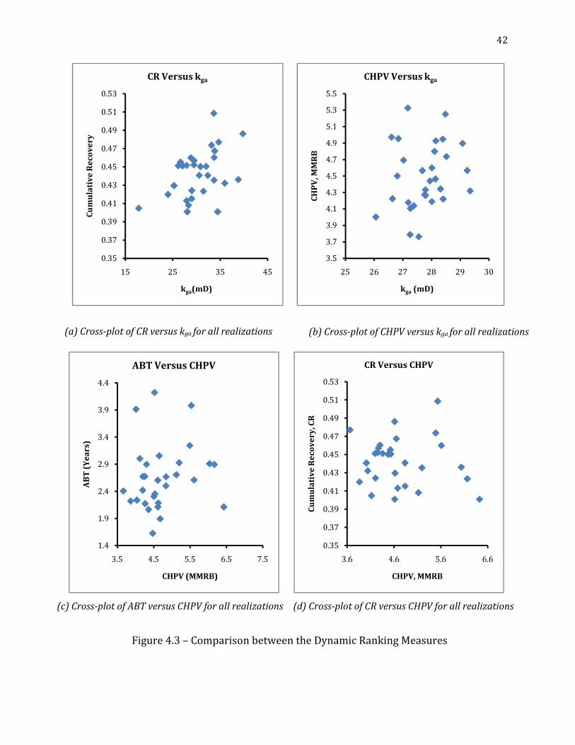
4.2.3 Relationship between Dynamic Ranking Criteria
Analysis of the results to understand the relationships between the dynamic
measures indicated that the cross-plot of CR versus average Geometric Average
Permeability showed fairly reasonable correlation (Figure 4.3a). It is observed that
realizations with high average permeability tend to produce high cumulative
recovery. However, because the Geometric Average Permeability measure is an
average value without any geospatial consideration, higher values of kga do not
necessarily guarantee higher cumulative recovery. Moreover, the cumulative
recovery takes into consideration reservoir rock and fluid properties, pressure and
time components which are not accounted for in the average Geometric Average
Permeability criteria. Hence it is in very rare cases that one would expect a
correlation between the two.
41
For these same reasons the average Geometric Average Permeability depicted a
poor correlation with the other dynamic measures. The cross-plot of CHPV versus
Geometric Average Permeability did not show any recognizable trend (Figure 4.3b).
Generally, poor correlation is observable between the dynamic ranking measures
(Figure4.3).
4.2.4 Application of Cumulative Recovery
It is worth noting that after utilizing STOOIP and three dynamic criteria, the original
30 realizations from SGSIM reduced to 12 (i.e. three realizations each from the
STOOIP, kga, CHPV and ABT). The simulation was run for an additional 5 years, for a
total of 15 years, and the cumulative recovery for each selected percentile (P10, P50
and P90) was recorded and analyzed. The realizations with high cumulative
recovery over the 10 – year run still maintained their ranks after the 15-year run.
From the static ranking criterion, the P50 realization (Realization 13) with the
medium STOOIP had the highest cumulative recovery and it was followed by the
P90 realization–23 (Figure 4.4a). The P10 realization had the lowest cumulative
recovery (CR). This observation suggests that a realization of high STOOIP rank does
not guarantee a high CR rank and vice versa; indicating the lack of a direct
relationship between the static and dynamic measures.
A reasonable trend is observable between the cumulative recovery criterion and the
other dynamic criteria after selecting the percentiles. Realization 25 corresponding
to the lowest (P10 realization) based on Geometric Average Permeability has the
lowest recovery followed by the P50 realization, with the highest cumulative
recovery being recorded by the P90 realization (Figure 4.4b). Similar observations
can be made for the selected P10, P50 and P90 realizations from both CHPV (Figure
4.4c) and ABT (Figure 4.4d) measures. Selected realizations with high CHPV and
ABT values have high cumulative recovery.
42
0.35
0.37
0.39
0.41
0.43
0.45
0.47
0.49
0.51
0.53
15 25 35 45
Cu
mu
lati
ve
Re
cov
ery
kga(mD)
CR Versus kga
3.5
3.7
3.9
4.1
4.3
4.5
4.7
4.9
5.1
5.3
5.5
25 26 27 28 29 30
CH
PV
, MM
RB
kga (mD)
CHPV Versus kga
1.4
1.9
2.4
2.9
3.4
3.9
4.4
3.5 4.5 5.5 6.5 7.5
AB
T (
Ye
ars
)
CHPV (MMRB)
ABT Versus CHPV
0.35
0.37
0.39
0.41
0.43
0.45
0.47
0.49
0.51
0.53
3.6 4.6 5.6 6.6
Cu
mu
lati
ve
Re
cov
ery
, CR
CHPV, MMRB
CR Versus CHPV
(a) Cross-plot of CR versus kga for all realizations (b) Cross-plot of CHPV versus kga for all realizations
Figure 4.3 – Comparison between the Dynamic Ranking Measures
(c) Cross-plot of ABT versus CHPV for all realizations (d) Cross-plot of CR versus CHPV for all realizations

43
0.460
0.465
0.470
0.475
0.480
0.485
0.490
0.495
0.500
0.505
0.510
0.515
P10 P50 P90
Cu
mu
lati
ve
Re
cov
ery
Percentile from STOOIP
CR Vs STOOIP
Real. 18
Real. 13
Real. 23
0.490
0.495
0.500
0.505
0.510
0.515
0.520
0.525
0.530
0.535
0.540
P10 P50 P90
Cu
mu
lati
ve
Re
cov
ery
Percentile from kga
CR Vs kga
Real. 9
Real. 30
Real. 25
0.470
0.475
0.480
0.485
0.490
0.495
0.500
0.505
0.510
0.515
0.520
0.525
P10 P50 P90
Cu
mu
lati
ve
Re
cov
ery
Percentile from CHPV
CR Vs CHPV
Real. 10
Real. 26
Real. 22
0.450
0.460
0.470
0.480
0.490
0.500
0.510
0.520
0.530
0.540
P10 P50 P90
Cu
mu
lati
ve
Re
cov
ery
Percentile from ABT
CR Vs ABT
Real. 7
Real. 10
Real. 6
(a) Cumulative Recovery versus Percentiles from
STOOIP
(b) Cumulative Recovery versus Percentiles from kga
(c) Cumulative Recovery versus Percentiles from CHPV (d) Cumulative Recovery versus Percentiles from ABT
Figure 4.4 – Cumulative Recovery after 15 years simulation versus percentiles from other
ranking measures
44
However, it is difficult to make the above observation by simply inspecting the ranks
in Table B2. Also, the cross-plots between the dynamic criteria for all the
realizations did not clearly show this trend. This therefore emphasizes the
significance of the percentile selection of the realizations based on the various
ranking criteria. Not only did it fairly represent the uncertainty associated with the
model selection, it also demonstrated the general trend of correlation between
cumulative recovery and the other dynamic measures.
Once more, the cumulative recovery (CR) after 15 years was used as filter to select
three realizations from the dynamic criteria. This was done by comparing the CR per
percentile for each dynamic measure (kga, CHPV and ABT) and selecting the one
with the highest recovery value. The figures showing the comparison are in
Appendix C. From this process, realizations 25, 10 and 9 corresponding to P10, P50
and P90 were selected to represent the dynamic criteria.
Finally, the CR values of the selected realizations from the static criterion were
compared with that of the dynamic. It was observed that the percentile realizations
of the dynamic criterion had higher cumulative recoveries than the static selected
ones (See Appendix C).
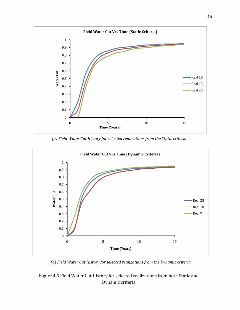
4.2.5 Application of Field Water Cut
At this stage, the original 30 realizations have been reduced to 6, that is, three each
from both static and dynamic measures. Field water cut which is a performance
criterion was used as the filter for this stage.
A 15-year simulation of a line drive waterflood was carried out on the two sets of
the three realizations selected (P10, P50 and P90) and the field water cuts were
analyzed. Figure 4.5 shows the field water cuts of the realizations selected from both
static and dynamic criteria. It was observed that the two sets of realizations
depicted extreme high and low cases of water cut. Realizations 18 and 9

45
corresponding to the static and dynamic measures came out with the highest water
cut whereas the lowest water cuts were shown by realizations 23 (static) and 10
(dynamic). By comparison, realization 18 from the static measure was observed to
have the earliest water breakthrough time and realization 9 from the dynamic
criteria, also produced the earliest breakthrough time. This explains why 18 and 9
have the highest water cut history in both cases.
The same observation was made for these two realizations when the field water oil
ratio was used to evaluate reservoir performance (See Appendix C). On the contrary,
when the field production rate was employed as a filter, those realizations with high
water cut in both cases depicted lower oil rates as compared to those with low
water cut history (See Appendix C).
4.3 HISTORY MATCHING
An attempt was made to history match the water cut from the field data. The
realizations from both static and dynamic measures whose water cut histories were
closest to that of the field under study were selected for this exercise. Due to the
high water cut observed during the period of history of the reservoir under study,
realizations 18 and 9 from the static and dynamic measures were selected for water
cut history matching. The history matching was carried out with minimal
adjustments to the reservoir input properties (Figure 4.6).
Thus, successful history match was obtained in a relatively short time using the
reduced set of realizations ranked by static and dynamic criteria. This type of
exercise demonstrates the need to analyze and rank realizations from static
modeling before using the reduced set of realizations in further fluid flow
simulations.
46
0
0.1
0.2
0.3
0.4
0.5
0.6
0.7
0.8
0.9
1
0 5 10 15
Wa
ter
Cu
t
Time (Years)
Field Water Cut Vrs Time (Static Criteria)
Real 18
Real 13
Real 23
0
0.1
0.2
0.3
0.4
0.5
0.6
0.7
0.8
0.9
1
0 5 10 15
Wa
ter
Cu
t
Time (Years)
Field Water Cut Vrs Time (Dynamic Criteria)
Real 25
Real 10
Real 9
(b) Field Water Cut History for selected realizations from the Dynamic criteria
(a) Field Water Cut History for selected realizations from the Static criteria
Figure 4.5 Field Water Cut History for selected realizations from both Static and
Dynamic criteria

47
0
0.1
0.2
0.3
0.4
0.5
0.6
0.7
0.8
0.9
1
1979 1984 1989 1994
Wa
ter
Cu
t
Time
Water Cut History Match
WCut History
Real 9 (Dynamic)
Real 18 (Static)
Figure 4.6 Water Cut History Match for selected realizations from both Static and
Dynamic Ranking Criteria

48
4.4 CHAPTER SUMMARY
The 30 realizations generated by SGSIM were reduced to 12 realizations by the
percentile selection from the static and dynamic ranking criteria. Application of the
cumulative recovery yielded three out of the nine realizations from the dynamic
criteria.
Two realizations selected from the analysis of both static and dynamic ranking
criteria were used to conduct a successful water cut history match.
The following chapter presents the conclusions made from the above results along
with some recommendations for further study.
49
CHAPTER FIVE – CONCLUSIONS AND RECOMMENDATIONS
The methodology, results and observations from this study are summarized in this
section. Major conclusions are presented along with a set of recommendations for
further study.
5.1 SUMMARY AND CONCLUSIONS
The objectives of the study are to build multiple equiprobable representations of the
reservoir with unique static and dynamic properties, and rank these realizations
with existing and new criteria to subsequently select a few for fluid flow simulation.
An actual field case study is used to evaluate the effectiveness of the new ranking
criteria.
A total of 30 equiprobable descriptions of the reservoir were built and ranked by
both static and dynamic measures. Apart from the horizontal and vertical
permeability distributions which were assumed to be uniform, the other
petrophysical properties were considered to be anisotropic. Two variogram
directions (i.e. major and minor directions of continuity) were employed to properly
capture the spatial relationships exhibited by the data. Subsequently, Sequential
Gaussian Simulation was used to generate 30 static models of the reservoir.
The STOOIP, geometric average permeability, connected hydrocarbon pore volume,
cumulative recovery and average breakthrough time were calculated for each
realization and used as the basis for ranking the realizations. The peculiarity of
these measures for each realization suggests the static and dynamic uniqueness of
the realizations generated.
In general, no strong correlation between the static (STOOIP) and dynamic (kga,
CHPV, ABT, and CR) measures was observed due to the lack of direct relationship
between the two. The 10th, 50th, and 90th percentiles of the realizations from each

50
ranking measure were utilized to significantly reduce the number of realizations by
60% for further studies.
Geometric Average Permeability, Average Breakthrough times, and Cumulative
Recovery are found to be effective dynamic measures for ranking reservoir
realizations. The dynamic ranking criteria were used to reduce the number of
realizations from 30 to 9 with uncertainty retained in the reduction. Then
cumulative recovery from the 15-year simulation of a line drive waterflood
provided three (3) realizations classified as low, medium and high.
Furthermore, from the water cut history of the 15 year waterflood, it can be
concluded that the realizations from the dynamic criteria provided a relatively
better reservoir performance match than that of the static criteria. This may be
attributed to the stronger relationship between the dynamic criteria and the
reservoir performance measures.
Based on the reservoir performance(cumulative recovery and water cut) after 15
years of water flooding, it is concluded that the ranking criteria evaluated in this
study can be effectively used to reduce the number of realizations in an integrated
study to a manageable size to be used for fluid flow simulation. The reduced set of
realizations can be employed for history matching and performance prediction.
Appendix D shows the workflow for building and ranking reservoir models on the
basis of this study.
5.2 RECOMMENDATIONS
The following is a set of recommendations provided to aid the building and ranking
of petroleum reservoir models.

51
It is recommended that a large number of equiprobable realizations are developed
for any reservoir study in order to adequately capture the uncertainty in the
reservoir characterization. For this work, due to computer hardware limitations
only 30 descriptions of the Tensleep reservoir were generated. However, for
extensive reservoir modeling with uncertainty assessment more than 30
realizations are recommended.
The capturing of reservoir heterogeneity is of great importance in reservoir
characterization. It is therefore recommended that fine grid reservoir models be
built in order to better account for small scale reservoir heterogeneities.
Fractures and faults among others play a key role in defining the reservoir structure
and drainage. Capturing these features in the characterization of the reservoir is
essential since they may affect the fluid flow dynamics. This study did not
incorporate the structural features of the reservoir; however, for a comprehensive
description of the reservoir, they should be integrated with the other static
properties.
No two petroleum reservoirs are the same. Due to this uniqueness of reservoirs, it is
a challenge to generally state whether a particular ranking criteria is best or worse.
It is therefore recommended that for any reservoir, an integrated ranking exercise
of both static and dynamic criteria be carried out in order to come up with a more
robust method. From this integrated ranking, a set of the tens to hundreds of
realizations could then be selected for fluid flow analysis, history matching and to
predict future reservoir performance.
There is lack of sufficient data in this study and hence appropriate conclusions could
not be drawn. However in any reservoir characterization exercise it is
recommended that adequate data be used in order to obtain more representative
results.

52
REFERENCES
Al-Khalifa, M.A., “Advances in Generating and Ranking Integrated Geological Models
for Fluvial Reservoir”, SPE 86999, presented at the SPE Asia Pacific Conference on
Integrated Modeling for Asset Management, held in Kuala Lumpur, Malaysia, 20-30
March 2004.
Ates, H., Bahar, A., Salem, E., Mohsen, C., and Akhil, D., “Ranking and Upscaling of
Geostatistical Reservoir Models Using Streamline Simulation: A field Case Study”,
SPE 81497, presented at the SPE 13th Middle East Oil Show and Conference, held in
Bahrain, 9-12 June 2003.
Ates, H., Kelka, M., and Datta-Gupta, A., “The description of Reservoir Properties by
integrating Geological, Geophysical and Engineering Data”, The University of Tulsa
and Texas A&M University, Joint Industry Project, 2003, pp. 3-16.
Ballin, P., Journel, A., and Aziz, K., “Prediction of Uncertainty in Reservoir
Performance Forecasting”, Journal of Canadian Petroleum Technology (JCPT), no. 4,
April 1992.
Datta-Gupta, A., and King, M.J., Streamline Simulation: Theory and Practice, SPE
Textbook Series, 2007.
Deutsch, C., Geostatistical Reservoir Modeling, Oxford University Press, 2002b.
Deutsch, C and Srinivasan, S., “Improved Reservoir Management through Ranking
Reservoir Models”, Society of Petroleum Engineers (SPE), Paper 35411, 1996.
Fenik, D.R., Nouri, A., and Deutsch, C.V., “Criteria for Ranking Realizations in the
Investigation of SAGD Reservoir Performance”, Paper 2009-191, presented at the
Canadian International Petroleum Conference, held in Calgary, Alberta, Canada, 16-
18 June 2009.
Garcia, R.G., “Reservoir Simulation of CO2 Sequestration and Enhanced Oil Recovery
in the Tensleep Formation, Teapot Dome Field”, Master of Science Thesis, Texas
A&M University, December 2005.
Gilman, J.R., Meng, A.Z., Uland, M.J., Dzurman, P.J., and Cosic, S., “Statistical Ranking
of Stochastic Geomodels Using Streamline Simulation: A Field Application”, SPE

53
77374, presented at SPE Annual Technical Conference and Exhibition, San Antonio,
Texas, USA. 2005
Goovaerts, P., Webster, R., and Dubois, J.P., 1997. “Assessing the risk of soil
contamination in the Swiss Jura using indicator geostatistics”, Environmental and
Ecological Statistics, 4(1): 31-48, Rothamsted Experimental Station, Harpenden,
Herts AL5 2JQ, UK. 1997.
Mclennan, J., and Deutsch, C., “Ranking Geostatistical Realizations by Measures of
Connectivity”, SPE 98168, presented at the SPE International Thermal Operations
and Heavy Oil Symposium, held in Calgary, Alberta, Canada, 1-3 November 2005.
Saad, N., and Kalkomey, C.T., “Ranking Geostatistical Models Using Tracer
Production Data”, SPE 35494, presented at the European 3D Reservoir Modeling
Conference, held in Stavanger, Norway, 16-17 April 1996.
Yadav, S., Bryant, S.L., and Srinivasan, S., “Ranking of Geostatistical Reservoir Models
and Uncertainty Assessment Using Real-Time Pressure Data”, SPE 100403,
presented at SPE Western Regional/AAPG Pacific Section/GSA Cordillera Section
Joint Meeting held in Alaska, USA, 8-10 May 2006.

54
APPENDIX A: Nomenclature
A = Area
h = thickness
φ= porosity
k = permeability, mD
µ = viscosity, cp
B = formation volume factor
Sw = Water saturation
Subscripts
o = oil
i = initial
c = cell number
n = total number of realizations
h = horizontal
v = vertical
eff = effective

55
APPENDIX B: Additional Figures and Tables for Chapter 3
Appendix B contains additional Figures and Tables discussed in Chapter 3 of this
study report.
Figure B1 – Location Map of the Teapot Dome Oil Field (Garcia, 2005).

56
(a) Raw Porosity data distribution over the reservoir (b) Porosity distribution for Realization 16
Figure B2: Porosity Distribution before and after SGSIM
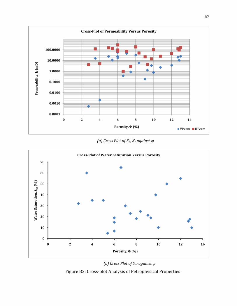
57
0.0001
0.0010
0.0100
0.1000
1.0000
10.0000
100.0000
0 2 4 6 8 10 12 14
Pe
rme
ab
ilit
y, k
(m
D)
Porosity, Ф (%)
Cross-Plot of Permeability Versus Porosity
VPerm HPerm
0
10
20
30
40
50
60
70
0 2 4 6 8 10 12 14
Wa
ter
Satu
rati
on
, Sw
i(%
)
Porosity, Ф (%)
Cross-Plot of Water Saturation Versus Porosity
(a) Cross Plot of Kh, Kv against φ
(b) Cross Plot of Swi against φ
Figure B3: Cross-plot Analysis of Petrophysical Properties

58
Table B1 Input Parameters for Variogram Computation and Modeling
Parameter Porosity Water
Saturation Horizontal
Permeability Vertical
Permeability Thickness
Number of Lags 35 20 20 20 35
Lag Separation 218 325 325 325 218
Lag Tolerance 75 110 105 105 75
Number of Directions 2 2 1 1 2
Major
Direction/
Omni-
directional
Azimuth 50 220 0 0 0
Dip 0 10.5 0 0 0
Tolerance 50 21 90 90 55
Bandwidth 1500 1500 2000 2000 1500
Minor
Direction
Azimuth 140 130 90
Dip 30 15 10
Tolerance 50 20 23
Bandwidth 1200 1000 1000
Nugget Effect 0 0 0 0 0
Number of Structures 1 1 1 1 1
Sill Contribution 10 360 5470 240 178.5
Minimum Range 228.9 455 650 585 152.6
Medium Range 1068.2 1755 1625 1235 915.6
Maximum Range 4959.5 3380 3445 2405 2365.3
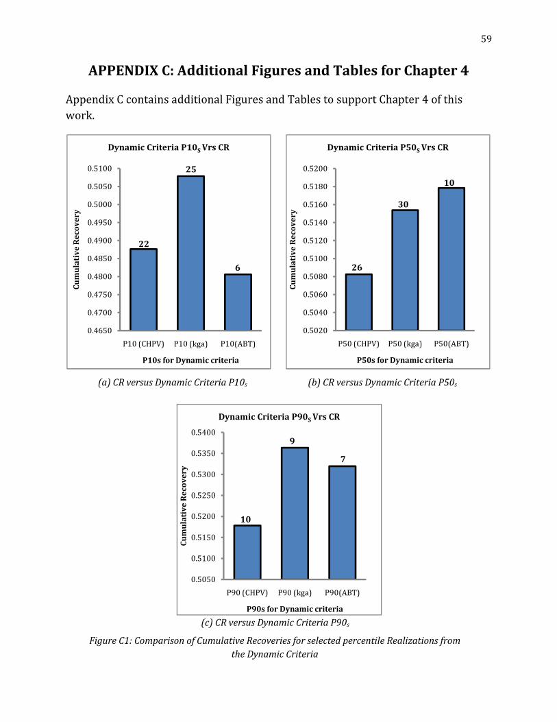
59
APPENDIX C: Additional Figures and Tables for Chapter 4
Appendix C contains additional Figures and Tables to support Chapter 4 of this
work.
0.4650
0.4700
0.4750
0.4800
0.4850
0.4900
0.4950
0.5000
0.5050
0.5100
P10 (CHPV) P10 (kga) P10(ABT)
Cu
mu
lati
ve
Re
cov
ery
P10s for Dynamic criteria
Dynamic Criteria P10S Vrs CR
6
25
22
0.5020
0.5040
0.5060
0.5080
0.5100
0.5120
0.5140
0.5160
0.5180
0.5200
P50 (CHPV) P50 (kga) P50(ABT)
Cu
mu
lati
ve
Re
cov
ery
P50s for Dynamic criteria
Dynamic Criteria P50S Vrs CR
10
30
26
0.5050
0.5100
0.5150
0.5200
0.5250
0.5300
0.5350
0.5400
P90 (CHPV) P90 (kga) P90(ABT)
Cu
mu
lati
ve
Re
cov
ery
P90s for Dynamic criteria
Dynamic Criteria P90S Vrs CR
7
9
10
(a) CR versus Dynamic Criteria P10s (b) CR versus Dynamic Criteria P50s
(c) CR versus Dynamic Criteria P90s
Figure C1: Comparison of Cumulative Recoveries for selected percentile Realizations from
the Dynamic Criteria
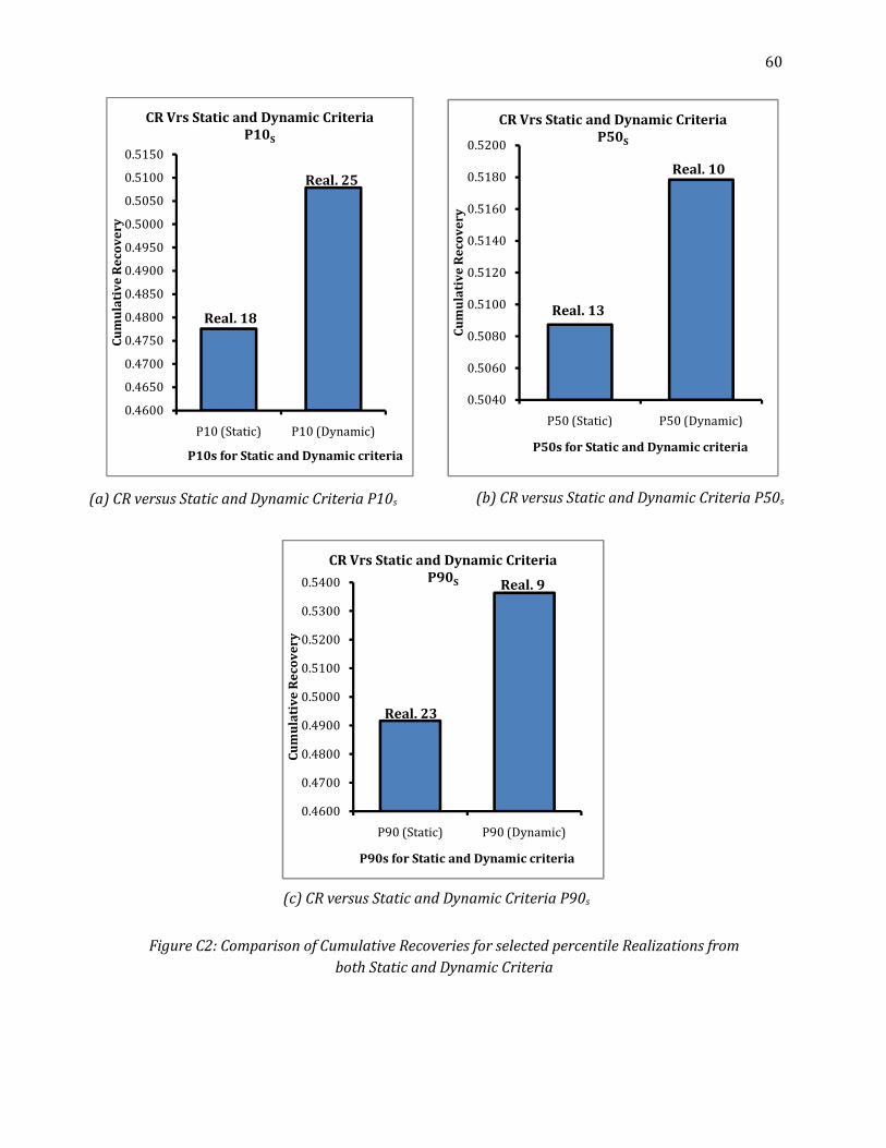
60
0.4600
0.4650
0.4700
0.4750
0.4800
0.4850
0.4900
0.4950
0.5000
0.5050
0.5100
0.5150
P10 (Static) P10 (Dynamic)
Cu
mu
lati
ve
Re
cov
ery
P10s for Static and Dynamic criteria
CR Vrs Static and Dynamic Criteria P10S
Real. 25
Real. 18
0.5040
0.5060
0.5080
0.5100
0.5120
0.5140
0.5160
0.5180
0.5200
P50 (Static) P50 (Dynamic)
Cu
mu
lati
ve
Re
cov
ery
P50s for Static and Dynamic criteria
CR Vrs Static and Dynamic Criteria P50S
Real. 10
Real. 13
0.4600
0.4700
0.4800
0.4900
0.5000
0.5100
0.5200
0.5300
0.5400
P90 (Static) P90 (Dynamic)
Cu
mu
lati
ve
Re
cov
ery
P90s for Static and Dynamic criteria
CR Vrs Static and Dynamic Criteria P90S Real. 9
Real. 23
(a) CR versus Static and Dynamic Criteria P10s (b) CR versus Static and Dynamic Criteria P50s
(c) CR versus Static and Dynamic Criteria P90s
Figure C2: Comparison of Cumulative Recoveries for selected percentile Realizations from
both Static and Dynamic Criteria

61
Table C1 - Values of each Criterion per Realization before Ranking
0
5
10
15
20
25
0 5 10 15
WO
R
Time (Years)
Field WOR Vrs Time (Static Criteria)
Real 18
Real 13
Real 23
0
2
4
6
8
10
12
14
16
18
20
0 5 10 15
WO
RTime (Years)
Field WOR Vrs Time (Dynamic Criteria)
Real 25
Real 10
Real 9
0
500
1000
1500
2000
2500
3000
0 5 10 15
Oil
Ra
te (
bb
l/d
ay
)
Time (Years)
Field Oil Rate Vrs Time (Static Criteria)
Real 18
Real 13
Real 23
0
500
1000
1500
2000
2500
0 5 10 15
Oil
Ra
te (
bb
l/d
ay
)
Time (Years)
Field Oil Rate Vrs Time (Dynamic Criteria)
Real 25
Real 10
Real 9
(a) Field WOR versus Time (Static Criteria)
(d) Field Oil Rate versus Time (Dynamic Criteria)
(b) Field WOR versus Time (Dynamic Criteria)
(c) Field Oil Rate versus Time (Static Criteria)
Figure C3: Analysis of selected realizations by WOR and Oil Rate performance measures

62
Real Number
STOOIP (MMSTB )
kga (mD)
CHPV (MMRB)
Average Breakthrough time (Years)
Cumulative Recovery (%)
1 4.535 28.06 4.615 2.111 40.09
2 4.438 26.63 4.522 4.224 45.52
3 5.459 31.45 6.166 2.895 42.34
4 4.493 30.83 4.474 1.625 45.02
5 4.244 39.75 4.612 2.603 48.62
6 5.788 34.46 6.424 2.111 40.09
7 5.190 33.16 5.490 3.245 47.37
8 4.917 33.63 5.534 3.982 50.85
9 3.638 34.67 3.663 2.406 47.71
10 5.413 28.81 5.610 2.611 46.00
11 4.737 17.80 4.119 3.003 40.48
12 4.670 27.90 4.678 1.894 41.30
13 4.533 27.90 4.503 2.306 45.16
14 4.799 33.84 4.649 3.055 46.74
15 3.950 32.37 4.012 3.913 44.07
16 4.886 33.69 5.197 2.925 43.55
17 5.052 28.32 5.122 2.706 40.81
18 4.077 29.01 4.204 2.672 42.41
19 4.171 27.04 4.357 2.063 45.11
20 4.279 23.99 3.863 2.220 41.99
21 4.270 33.72 4.301 2.898 46.03
22 3.998 35.95 4.039 2.236 43.21
23 5.313 38.80 6.038 2.910 43.62
24 4.522 29.46 4.254 2.674 45.22
25 4.282 26.16 4.196 2.419 45.13
26 4.514 32.02 4.532 2.351 45.05
27 4.526 30.58 4.835 2.501 44.08
28 4.760 25.26 4.624 2.185 42.95
29 4.891 28.98 4.838 2.668 41.53
30 4.548 29.46 4.266 2.172 45.69
Table C2 – Ranking Results for each Criterion

63
STATIC RANKING DYNAMIC RANKING
Rank Real Number STOOIP
(MMSTB)
Real
Number
kga
(mD) Real
Number
CHPV (MMRB)
High
1 6 5.788 5 39.748 6 6.424
2 3 5.459 23 38.802 3 6.166
3 10 5.413 22 35.945 23 6.038
4 23 5.313 9 34.665 10 5.610
5 7 5.190 6 34.464 8 5.534
6 17 5.052 14 33.841 7 5.490
7 8 4.917 21 33.715 16 5.197
8 29 4.891 16 33.693 17 5.122
9 16 4.886 8 33.634 29 4.838
10 14 4.799 7 33.159 27 4.835
Medium
11 28 4.760 15 32.372 12 4.678
12 11 4.737 26 32.021 14 4.649
13 12 4.670 3 31.450 28 4.624
14 30 4.548 4 30.833 1 4.615
15 1 4.535 27 30.576 5 4.612
16 13 4.533 30 29.463 26 4.532
17 27 4.526 24 29.463 2 4.522
18 24 4.522 18 29.008 13 4.503
19 26 4.514 29 28.978 4 4.474
20 4 4.493 10 28.807 19 4.357
Low
21 2 4.438 17 28.316 21 4.301
22 25 4.282 1 28.065 30 4.266
23 20 4.279 12 27.902 24 4.254
24 21 4.270 13 27.902 18 4.204
25 5 4.244 19 27.044 25 4.196
26 19 4.171 2 26.633 11 4.119
27 18 4.077 25 26.157 22 4.039
28 22 3.998 28 25.258 15 4.012
29 15 3.950 20 23.985 20 3.863
30 9 3.638 11 17.803 9 3.663
Table C2 Cont. After Ranking

64
DYNAMIC RANKING
Rank Real
Number
Average Breakthrough Time (Years)
Real
Number
Cumulative Recovery (%)
High
1 2 4.224 8 50.85
2 8 3.982 5 48.62
3 15 3.913 9 47.71
4 7 3.245 7 47.37
5 14 3.055 14 46.74
6 11 3.003 21 46.03
7 16 2.925 10 46.00
8 23 2.910 30 45.69
9 21 2.898 2 45.52
10 3 2.895 24 45.22
Medium
11 17 2.706 13 45.16
12 24 2.674 25 45.13
13 18 2.672 19 45.11
14 29 2.668 26 45.05
15 10 2.611 4 45.02
16 5 2.603 27 44.08
17 27 2.501 15 44.07
18 25 2.419 23 43.62
19 9 2.406 16 43.55
20 26 2.351 22 43.21
Low
21 13 2.306 28 42.95
22 22 2.236 18 42.41
23 20 2.220 3 42.34
24 28 2.185 20 41.99
25 30 2.172 29 41.53
26 1 2.111 12 41.30
27 6 2.111 17 40.81
28 19 2.063 11 40.48
29 12 1.894 1 40.09
30 4 1.625 6 40.09
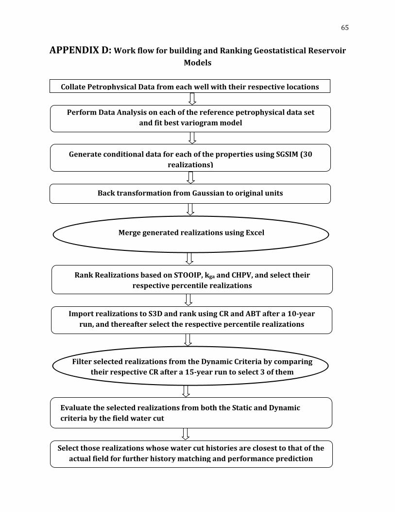
65
APPENDIX D: Work flow for building and Ranking Geostatistical Reservoir
Models
Collate Petrophysical Data from each well with their respective locations
Generate conditional data for each of the properties using SGSIM (30
realizations)
Back transformation from Gaussian to original units
Rank Realizations based on STOOIP, kga and CHPV, and select their
respective percentile realizations
Evaluate the selected realizations from both the Static and Dynamic
criteria by the field water cut
Merge generated realizations using Excel
Import realizations to S3D and rank using CR and ABT after a 10-year
run, and thereafter select the respective percentile realizations
Filter selected realizations from the Dynamic Criteria by comparing
their respective CR after a 15-year run to select 3 of them
Select those realizations whose water cut histories are closest to that of the
actual field for further history matching and performance prediction
Perform Data Analysis on each of the reference petrophysical data set
and fit best variogram model