building a simple spectrum analyzer with...

FACULTY OF ENGINEERING AND SUSTAINABLE DEVELOPMENT

Building a simple spectrum analyzer with dsPIC30F4013

Lian Xiangyu & Jiang Chunguang

06/2011

Bachelor’s Thesis in Electronics

Bachelor`s Thesis in Electronics

Examiner: Niklas Rothpfeffer

Supervisor: Efrain Zenteno

Lian Xiangyu & Jiang Chunguang Building a simple spectrum analyzer with dsPIC30F4013

i

Abstract

FFT-based digital spectral analyzer has become more and more widely used as a result of the

development of Digital Signal Processing (DSP) techniques. Modern Analog-to-Digital

Converters (ADC) and processors have made it possible to make fast measurements with a

limited number of hardware.

In this thesis, a design of a simple low-cost FFT-based digital spectrum analyzer was

presented. The author discusses the design of each components of the system in qualitatively

and quantitatively. The report presents the whole system design in detail which contains filter

design, micro-controller design, UART transmission design and MATLAB GUI design. Some

satisfying measurement result of the system were presented in the paper. The system can

provide fast measurement with good accuracy. But the measured result has a limited range

and resolution of the display is not very high. At last, the advantages and disadvantages of the

system was discussed which is considered as guidelines for further work.


ii

Preface

In the period to complete the thesis work, there are many frustrations happened. And we were

dejected and confused at one time. Luckily, thanks to our patient supervisor Efrain Zenteno

who helped us to solve different problems. Also thanks to Niklas Rothpfeffer to provide us

get equipments again and again, thanks to all the teachers teach us the knowledge so that we

can finish our thesis. Besides, thanks to our friends who have always been encouraging and

supporting us. At last, thanks to our parents provide us the chance to study in Sweden.


iii

Table of contents

Building a simple spectrum analyzer with dsPIC30F4013 ................................................................ 1

Abstract .................................................................................................................................................... i

Preface ..................................................................................................................................................... ii

Table of contents .................................................................................................................................... iii

1. Introduction ..................................................................................................................................... 1

1.1 Background .............................................................................................................................. 1

1.2 Research Aims ......................................................................................................................... 4

2. Theory ............................................................................................................................................. 5

2.1 FFT ................................................................................................................................................ 5

2.2 D-L Lemma ................................................................................................................................... 5

2.3Twiddle Factors .............................................................................................................................. 6

2.4The Butterfly Diagram ................................................................................................................... 7

2.5 Low Pass Filter .............................................................................................................................. 8

3. Process ........................................................................................................................................... 11

3.1 Analog low-pass filter design ................................................................................................. 11

3.2 System set up ......................................................................................................................... 13

3.3 ADC configuration ................................................................................................................. 14

3.4 DSP engine configuration ...................................................................................................... 16

3.5 UART configuration .............................................................................................................. 17

3.6 Display software configuration .............................................................................................. 19

4 Result ............................................................................................................................................. 20

4.1 Final system ........................................................................................................................... 20

4.2 Measurement results............................................................................................................... 20

5 Discussion ..................................................................................................................................... 24

5.1 Discussion of the method ....................................................................................................... 24

5.2 Discussion of the final system ................................................................................................ 24

6 Conclusion ..................................................................................................................................... 26


iv

References ............................................................................................................................................. 27

Appendix A Code of dsPIC30F4013 .................................................................................................. C1

Appendix B Code of MATLAB Display............................................................................................ C5


1

1. Introduction

1.1 Background

A spectrum analyzer is basically supposed to measure a power of the signal versus its

frequency. This job was done by using analog Swept Spectrum Analyzer (SSA) in the old

times [1]. But nowadays, a modern FFT-based digital spectral analyzer and do the same with

lesser requirement and provide better results [2]. This has made the spectral analyzing more

convenient without hurting its accuracy [3] [4]. FFT-based spectrum analysis (FFTSA) has

become a widely used method for many implementations [5].

As Figure 1 shows, the analyzed signal will be presented in frequency domain instead of time

domain. Letting the horizontal axis illustrates the frequency and the vertical axis illustrates the

amplitude of the signal [6].

Figure 1. Imagination of spectrum for signal


2

Figure 2. Simplified Spectrum Analyzer Block Diagram.

Figure 2 presents the basic architecture of both SSA and Digital Spectral Analyzer. It

explains theoretically how a basic spectral analyzer works [1].

In the analog module, the analog input signal was first sent into an analog down-converter. At

the same time, the local oscillator will provide a sinusoidal signal as reference signal to the

down-converter. After multiplying these two signals together, the down-converter will

produce a signal with suitable frequency for subsequent processing [1]. This output signal is

called Intermediate Frequency (IF) signal. The frequency of the reference signal generated by

the LO is controlled by the frequency range of the FFT through a controller in a Digital

Spectral Analyzer. However, it is swept linearly over the frequency band or span to be

measured [1].

In the digital module, the IF signals is sent into the ADC. The ADC will converter the analog

signal into digital form. And the collected data is sent into DSP. The DSP will compute the

FFT and output data to digital display. The processor should also control the LO with some

algorithms. Most simple processors have the capability to do the job.


3

Figure 3. Detailed architecture of a Digital Spectral Analyzer.

Figure 3 presents the detailed architecture of a simple Digital Spectral Analyzer which is

studied in this paper [7]. This figure of Digital Spectral Analyzer shows more information

about the digital module part than Figure 1 because it shows the FFT process.

In the analog module, the analog input signal is first applied to a sharp roll-off analog low-

pass filter. The bandwidth of the low-pass filter is controlled by the controller in the processor.

Then the output of the filter is applied to the digital module.

In the digital module, the analog signal is first applied to the ADC. The working frequency of

the ADC is also controlled by the processor which can change the sampling frequency

generated from the reference oscillator. The sampling rate of the ADC must be larger than

twice the bandwidth of the low-pass filter to make sure no aliasing occurs [8]. At the same

time, the reference signal with sampling frequency chosen is read by a Weighting Function

ROM and converted to digital data. Then the multiplier will collect both data from the ADC

and Weighting Function ROM to multiply them together to compute the FFT. Then data is

transferred into the processor.


4

The memory of the processor will add the numbers stored in the memory with coefficients

(sin and cos) read from ROM and restore the result [7]. Then it will add and store again under

the control of the arithmetic unit until the process is done. The arithmetic unit also decides

how the controller should control the bandwidth of the analog low pass filter and the sampling

frequency of the reference signal. At last the processor can output the results in memory to the

display device.

1.2 Research Aims

The aim of the research is to design a simple Digital Spectral Analyzer with a limited number

of hardware from HIG. The processor is a dsPIC4013 micro-controller. It will compute the

analog to digital conversion and FFT. Then send the result through a PIC kit2 to a PC which

is considered to a display device. By building a GUI with MATLAB, the PC will display the

result graphically. Software used is MPLAB IDE with micro c30 complier and MATLAB

The system will analyze signal from 0 to 41 kHz. It should have some capabilities as the

equipment used in laboratory works. The system could be powered by batteries and easy to

carry, making it a convenient tool for simple signal analysis.


5

2. Theory

2.1 FFT

The FFT refers to a "Fast Fourier Transform" which is a very efficient "Discrete Fourier

Transform"(DFT). The reason of using FFT instead of DFT is that it saves time. For example,

a straight DFT with N samples requires N2

complex multiplications, while a FFT with the

same samples requires only Nlog2N complex multiplications [9].

The reason why FFT is fast can be explained by discussing its three characteristics:

“Danielson-Lanczos Lemma” (D-L Lemma), “twiddle factors" and” Butterfly Diagram”.

2.2 D-L Lemma

The DFT process follows equation 1 [7]:

1.....2,1,0

)()(

21

0

Nk

enfkF N

knjN

n

(1)

Where F(k) is the power of the signal at frequency elements k, and f(n) are N samples of the

input function.

In a D-L Lemma, the first step is to break down the expression into two parts: even terms and

odd terms. It becomes equation 2:

N

njN

knjN

k

N

knjN

k

N

knjN

n

eenfenf

OEenfkF

2

2

21

2

0

2

21

2

0

21

0

)12()2(

)()(

(2)

Where n

NN

nj

We

2

, known as twiddle factors.


6

Then F (k) is broken down in this order until the expression runs out of samples, which means

0

0

0

k

e [9]. This is the reason why the number of samples (N) in the FFT needs to be the

power of 2.

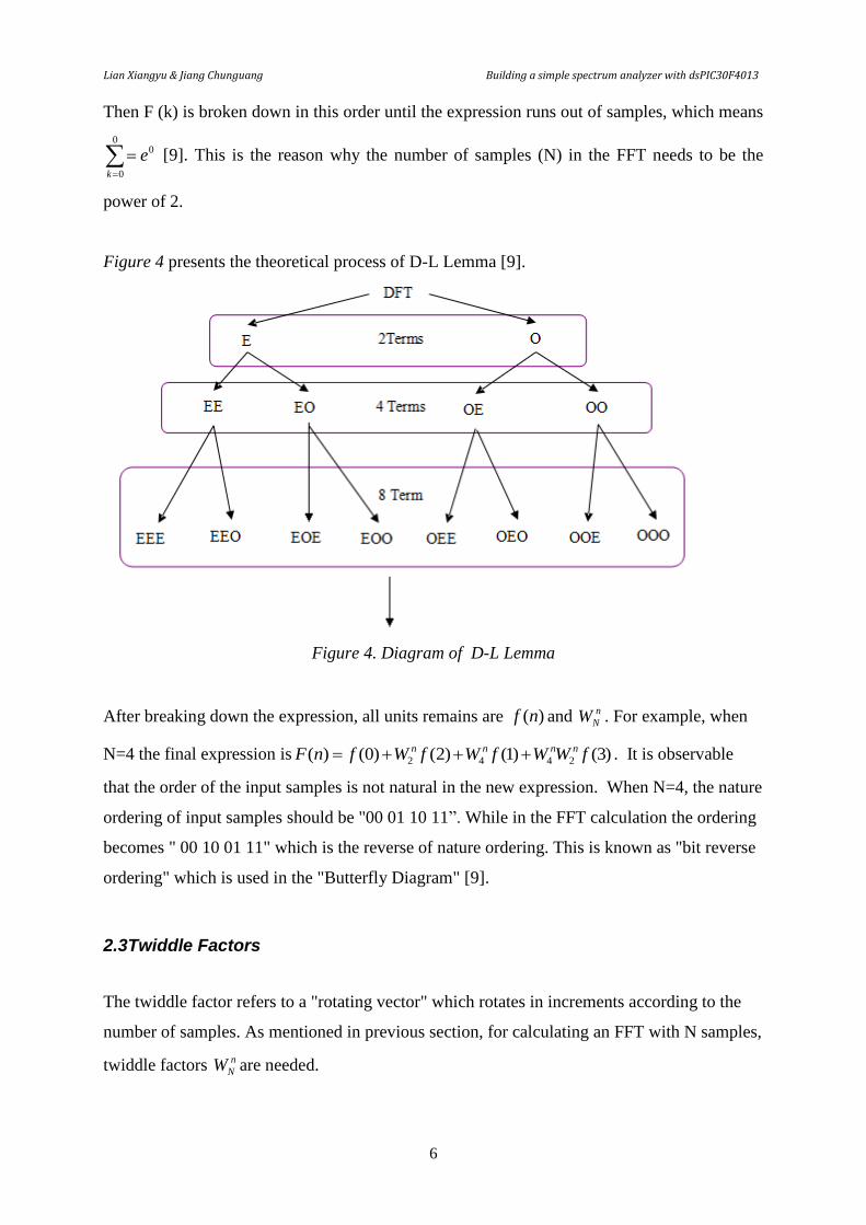
Figure 4 presents the theoretical process of D-L Lemma [9].

Figure 4. Diagram of D-L Lemma

After breaking down the expression, all units remains are )(nf and n

NW . For example, when

N=4 the final expression is )3()1()2()0()( 2442 fWWfWfWfnF nnnn . It is observable

that the order of the input samples is not natural in the new expression. When N=4, the nature

ordering of input samples should be "00 01 10 11”. While in the FFT calculation the ordering

becomes " 00 10 01 11" which is the reverse of nature ordering. This is known as "bit reverse

ordering" which is used in the "Butterfly Diagram" [9].

2.3Twiddle Factors

The twiddle factor refers to a "rotating vector" which rotates in increments according to the

number of samples. As mentioned in previous section, for calculating an FFT with N samples,

twiddle factors n

NW are needed.


7

Figure 5 presents how to generate twiddle factors for a certain number of samples [9].

Figure 5. Diagram of Twiddle Factors

Figure 5 indicates that the large number of samples in FFT, the more twiddle factors needed.

And the twiddle factor has redundancy in values as the vector rotates around [9]. This means

Nn

N

n

N WW . Also, the values of twiddle factors with 180 degrees out of phase are the negative

of each other which means 2 -N

n

N

n

N WW

. The "Butterfly diagram" takes advantage of these

characteristic of the twiddle factor, making the FFT realizable.

2.4The Butterfly Diagram

The Butterfly Diagram is an efficient FFT algorithm based on D-L Lemma and the twiddle

factors. For an FFT with N samples, the Butterfly Diagram will contain N2log stages. The

first stage of the diagram is presented in figure 6 [9].

Figure 6. First stage of Butterfly Diagram


8

The -1 in the figure 7 refers to 0

2

1

2 WW as mentioned in previous section. Then the next

stage will connect the upper and lower legs of the butterflies presented in figure 7 [9].

Figure 7. Butterfly Diagram

The diagram will continue computing in this way until the N2log stage is done. Note that if

the input samples are in bit reversed ordering, the output will be natural ordering.

2.5 Low Pass Filter

In signal processing, filter is a device that can remove these unwanted components in a

signal . It can be either analog or digital, discrete-time or continuous-time, linear or non-linear,

time-invariant or time-variant, passive or active. In this work, an analog continuous-time

active low-pass filter is chosen. As it require lesser components and easy to be built. The

purpose of using such a filter in this work is to remove signals that have frequency higher

than half of the sampling frequency. So the analog low-pass filter is an anti-aliasing

component of the system.

The following figures are representative of a low pass filter has different type of filter

response.


9

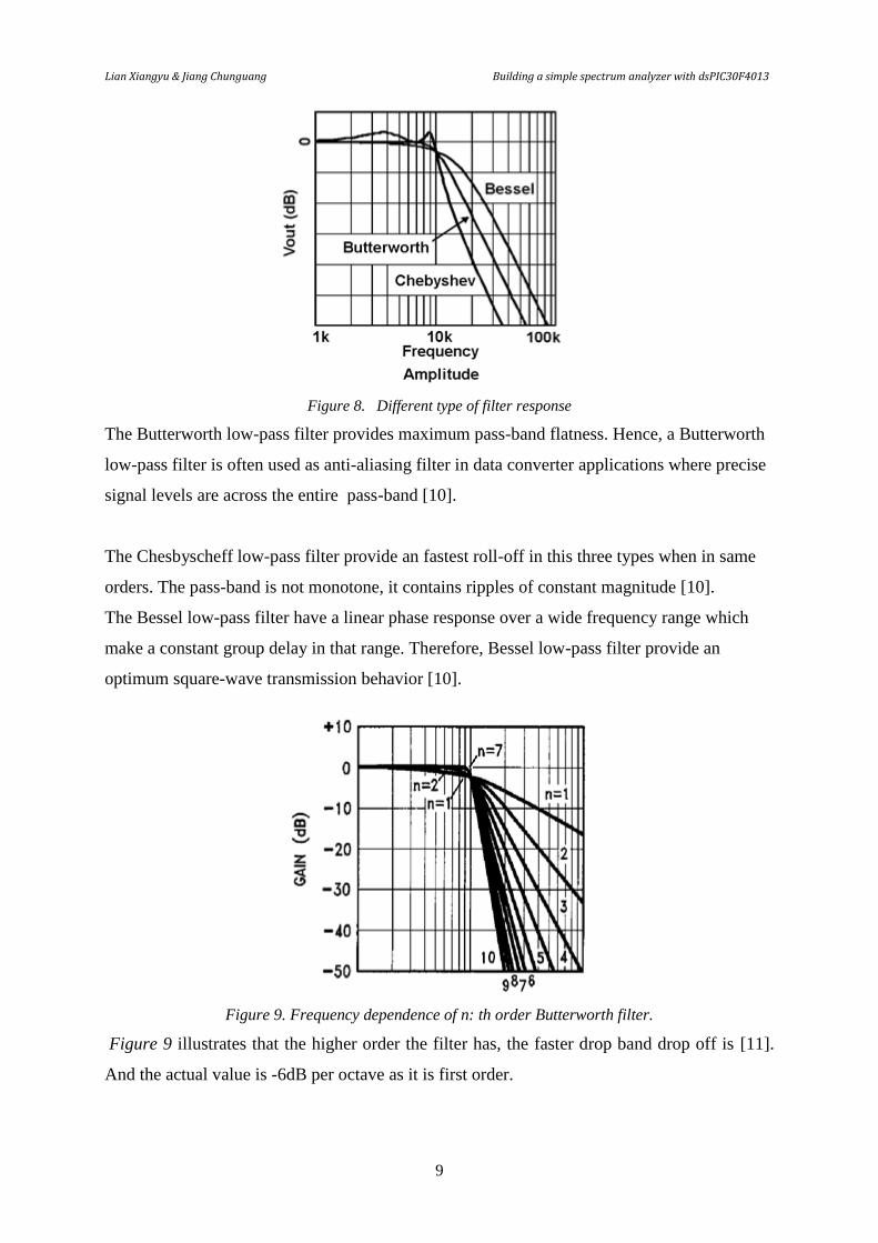
Figure 8. Different type of filter response

The Butterworth low-pass filter provides maximum pass-band flatness. Hence, a Butterworth

low-pass filter is often used as anti-aliasing filter in data converter applications where precise

signal levels are across the entire pass-band [10].

The Chesbyscheff low-pass filter provide an fastest roll-off in this three types when in same

orders. The pass-band is not monotone, it contains ripples of constant magnitude [10].

The Bessel low-pass filter have a linear phase response over a wide frequency range which

make a constant group delay in that range. Therefore, Bessel low-pass filter provide an

optimum square-wave transmission behavior [10].

Figure 9. Frequency dependence of n: th order Butterworth filter.

Figure 9 illustrates that the higher order the filter has, the faster drop band drop off is [11].

And the actual value is -6dB per octave as it is first order.


10

The Sallen-key topology can provide high accuracy, unity gain, and low Q(Q<3).

The Multiple Feedback topology is commonly used in filters that have high Q and require a

high gain [10].

2

2121

2

211 )(1

1)(

sCCRRsRRCsA

cc (3)

21

211

2

2

2

121

2,14

4

CCf

CCbCaCaR

c

(4)

where

2121

2

1

2111 )(

CCRRb

RRCa

c

c

(5)

In order to obtain real values under the square root, C2 must satisfy the following condition:

2

1

112

4

a

bCC (6)

Table 1 presents the coefficients of a second order filter

SECOND-ORDER BESSEL BUTTERWORTH TSCHEBYSCHEFF

a1 1.3617 1.4142 1.065

a1 0.618 1 1.9305

Q 0.58 0.71 1.3

Table.1 second order filter coefficients

The cut-off frequency of the second-order filter follows equation 5:

22112

1

CRCRfc

(7)


11

3. Process

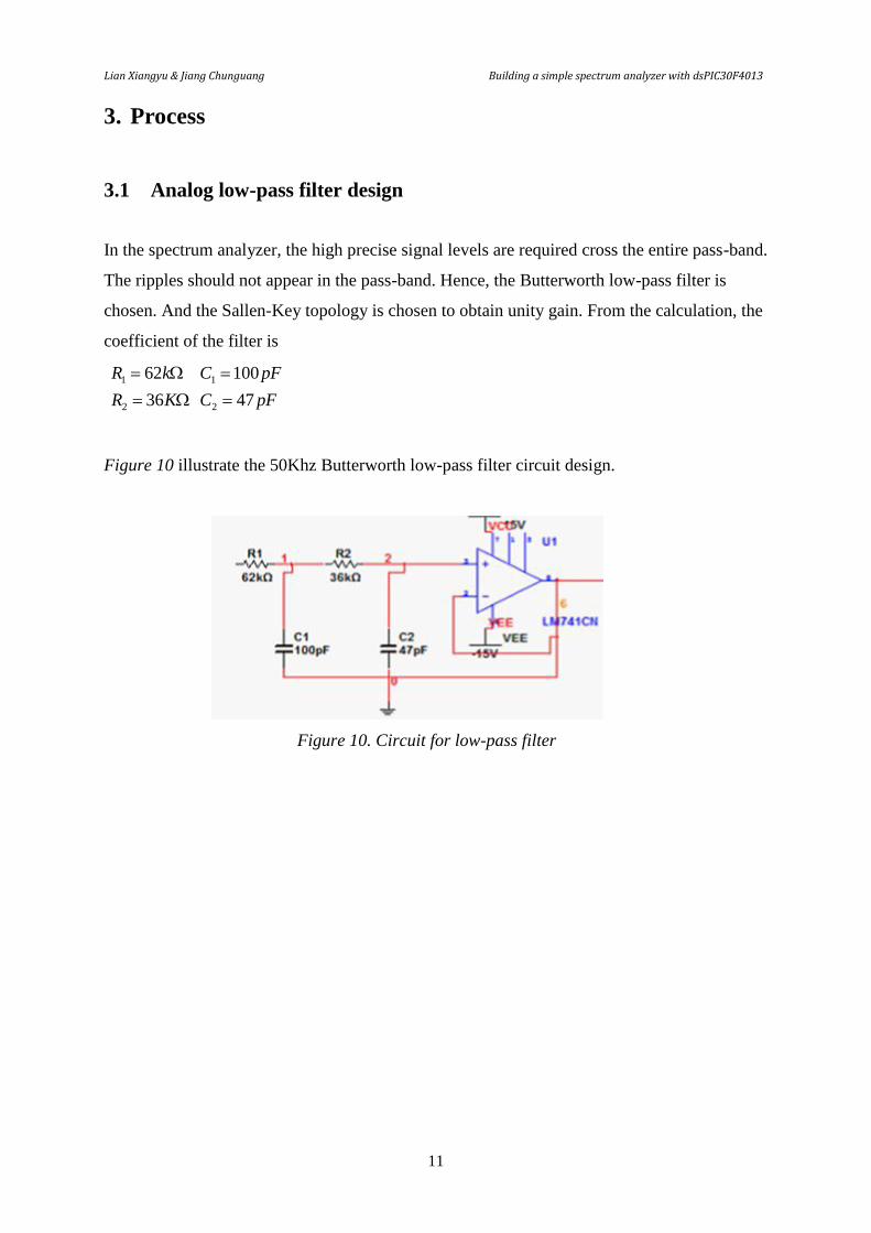
3.1 Analog low-pass filter design

In the spectrum analyzer, the high precise signal levels are required cross the entire pass-band.

The ripples should not appear in the pass-band. Hence, the Butterworth low-pass filter is

chosen. And the Sallen-Key topology is chosen to obtain unity gain. From the calculation, the

coefficient of the filter is

KR

kR

36

62

2

1

pFC

pFC

47

100

2

1

Figure 10 illustrate the 50Khz Butterworth low-pass filter circuit design.

Figure 10. Circuit for low-pass filter


12

Connect the circuit as the same to figure 10. Table 2 below shows the practical test results.

frequency Output(1) Output(2

combination)

Output(3

combination) Gain(dB)

50hz 1.038 1.065 1.058 0.32394707025

100hz 1.044 1.075 1.076 0.37400997332

1khz 1.038 1.075 1.076 0.32394707025

2k 1.044 1.069 1.065 0.37400997332

3k 1.044 1.069 1.065 0.37400997332

4k 1.044 1.068 1.053 0.37400997332

5k 1.044 1.053 1.047 0.37400997332

6k 1.044 1.05 1.022 0.37400997332

7k 1.044 1.052 1.011 0.37400997332

8k 1.044 1.052 1.01 0.37400997332

9k 1.044 1.045 0.989 0.37400997332

10k 1.044 1.045 0.988 0.37400997332

15k 1.044 1.038 0.977 0.37400997332

20k 1.025 1.004 0.955 0.21447730784

25k 1.013 0.956 0.855 0.11218890721

30k 0.975 0.859 0.756 -0.21990768603

35k 0.913 0.756 0.62 -0.79058444931

40k 0.856 0.639 0.402 -1.3505247065

45k 0.781 0.539 0.356 -2.1469793225

50k 0.7 0.431 0.256 -3.0980391997

60k 0.55 0.3 0.156 -5.1927462101

70k 0.438 0.2 0.101 -7.1705177899

80k 0.356 0.15 0.05 -8.9710000405

90k 0.294 0.125 0.032 -10.633053392

100k 0.244 0.106 0.014 -12.252203473

200k 0.081 0.069 0.102 -21.830299622

1M 0.106 0.069 0.092 -19.493882695

Table 2. Result of practical test for filter


13

Figure 11. the result of practical test for filter

From table 2 and figure 11 we can indicate that the aim of build a 50Khz Butterworth low-

pass filter achieved.

3.2 System set up

First of all, a system clock needs to be configured. Adjusting the clock of the microcontroller

is done by setting up the oscillator configuration register. In this work can be easily done by

using a macro: _FOSC. Then Oscillator Control Register (OSCCON) and FRC Oscillator

Tuning Register (OSCTUN) were not written to as the FRC oscillator for this work do not

need specification. So the system clock is configured as below:

_FOSC (CSW_FSCM_OFF & FRC)

Set up Internal Fast RC Oscillator as source oscillator. No PLL mode enabled and disable

clock switch. The oscillator is working at 7.37MHz so the frequency of the instruction cycle

is 1.84MHz.


14

Then some other registers were written to provide necessary configuration.

_FWDT (WDT_OFF)

Watch-Dog Timer is disabled.

_FBORPOR (MCLR_EN & PWRT_OFF)

Enable MCLR reset pin is enabled and the power-up timers is disabled.

_FGS (CODE_PROT_OFF)

Code protection is disabled.

3.3 ADC configuration

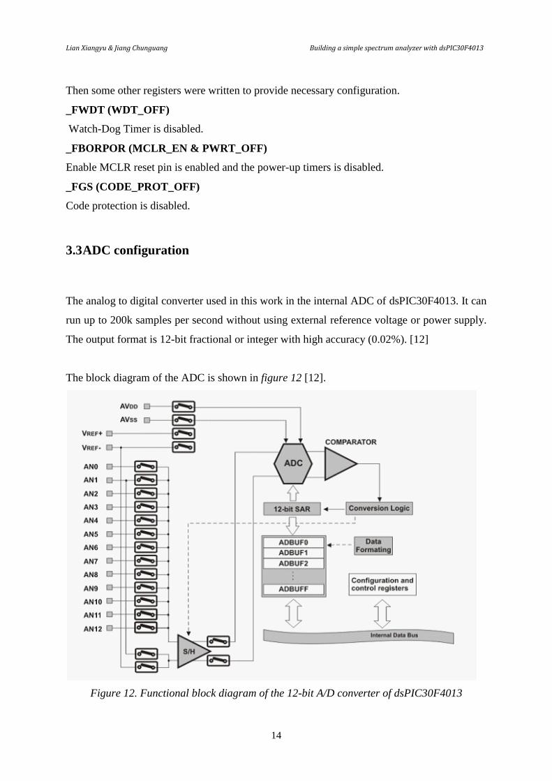
The analog to digital converter used in this work in the internal ADC of dsPIC30F4013. It can

run up to 200k samples per second without using external reference voltage or power supply.

The output format is 12-bit fractional or integer with high accuracy (0.02%). [12]

The block diagram of the ADC is shown in figure 12 [12].

Figure 12. Functional block diagram of the 12-bit A/D converter of dsPIC30F4013


15

AN0 to AN12 are input channels. Only one of them is used in this work. Vref+ and Vref-

refers to external reference voltage which is not used in this work. ADBUF0 to ADBUFF

refers are output buffers of the ADC. Only ADBUF0 is used in this work for easier data

collecting.

The pin out of dsPIC30F4013 is presented in figure 13 [12].

Figure 13. Pin out of dsPIC30F4013

To setup a ADC that satisfy the system, the following status registers in the dsPIC30F4013

need to be written: ADCON1, ADCON2, ADCON3, ADPCFG, TRISB, ADCHS and

ADCSSL. The ADC was set to work with following characteristics.

A. Generate input analog signal from port B 10, channel AN10.

B. The ADC runs with MUX A multiplexer. Positive and negative input of MUX A were set

to be AN10 and ground.

C. The sampling process takes 1 TAD and the conversion takes 14 TAD.

D. The sampling frequency is of ADC is 89 kHz as the ADCS bits on ADCON3 were set to be

two. From 2

)12( CY

AD

TT , knowing that TCY=1/FCY=0.54us, Tad is 0.81 us.

So FAD=1/15*TAD=82 kHz.

E. No scan on the ADC input


16

F. Reference voltage of ADC is AVdd (5V) and AVss(ground).

G. An interrupt will occur upon completion of each conversion. This will make all the output

data of ADC stored in ADCBUF0.

H. The output data format is fractional. And the ADC will auto start sampling and conversion

after the ADC is on.

3.4 DSP engine configuration

The core of DSP used in this work is the multiplier. It computes the FFT arithmetic. The first

step to set up the DSP is to declare the array of twiddle factors in program memory. Then

declare the array of ADC output array in the Y data bus of the multiplier.

As mentioned in theory, an FFT process with N samples needs only N/2 twiddle factors. As

each element in twiddle factors has one "real" part and one "imag" part. So totally N

fractional numbers written in 2N bytes were contained in the Twiddle Factor array. This array

is considered as constants and stored in program memory. The PSV mode will generate these

constant to the X data bus of multiplier when computing the FFT which will reduce the

processing time. The PSVPAG register which is used to translate 24-bit data in program

memory to 16-bit data in multiplier can be automatically written by a macro. The final code

of this step is as follows.

const fractcomplex twiddleFactors[] __attribute__ ((space(auto_psv), aligned

(FFT_N*2)));[13]

The array on input sample is the array of ADC output data. For an FFT with N samples, the

input array contain N elements which is 2N fractional numbers written in 4N bytes. To collect

data from ADC output buffer , the "real" part of the array needs to be declared equal to

ADCBUF0. Programmed as ADCoutput[i].real=ADCBUF0, where i is an integer which

increase from zero to N-1. Then declare the array to be transferred to y data bus of the

multiplier. The code for this step is:


17

fractcomplex ADCoutput[FFT_N]

__attribute__((space(ymemory),far,aligned(FFT_N*2*2)))[13]

As the output data range is [-1,1] and the multiplier requires data range to be [-0.5,0.5][11].

The "real" parts of the array need to be scale by 0.5 for further processing. This is done by

shift the ADC output data one bit to the right. The "imag" part of the array also needs to be

declared to be 0 as the input signal does not contain an imaginary part.

ADCoutput[i].real = ADCoutput[i].real>>1; ADCoutput[i].imag = 0x0000;

where i is an integer which increase from zero to N-1.

The FFT process is done with the macro

FFTComplexIP (LOG2_N, &sourcevector, (fractcomplex *) __builtin_psvoffset

(&twiddleFactors[0]), (int)__builtin_psvpage(&twiddleFactors[0]));[13]

With this macro, the multiplier will generate input samples from the "sourcevector" and

twiddle factors from program memory. LOG2_N refers to the number of stages the Butterfly

will process. The output result with frequency component is in bit reversed ordering and

stored back into the "sourcevector". As the real frequency of the signal is calculated in further

processing, the "sourcevector" needs to be translated into natural ordering. This is done by the

macro BitReverseComplex(LOG2_N, &sourcevector)[12]. As the "sourcevector" still

contains a "real" part and an "imag" part , and the final output is the power of the signal in

"real" only. The power is calculated as 22 IRP . This is done by the macro

SquareMagnitudeCplx(FFT_N, (fractcomplex *) &sourcevector[0], (fractional*)

&sourcevector[0].real);[13]

The value of the power is stored in "real" part of the "sourcevector" after this step. And the

FFT process is considered to be over.

3.5 UART configuration

The UART part of the system is designed to connect the dsPIC30F4013 to the PC. Output

data of DSP model is transferred through the transmitter. The tool used for connection is a

PICkit2.


18

The UART model within dsPIC30F4013 is designed with following characteristics [12]:

A . Use U1TX as transmit channel.

B. 8-bit data communication with no parity.

C. A transmission interrupt is generated when a character is transferred to the transmit shift

register and the transmit buffer becomes empty.

D. UART model continue operation in IDLE mode.

E. UART loop back mode is disabled.

F. UART baud rate is 2300 bytes per second.

The transmitted data is displayed on the software named PICkit 2 programmer. This is a

powerful software when a PICkit2 is used as the UART tool. This software is achievable from

the Microchip official website. The user interface of the software is presented in figure 14.

Figure 14. User interface of PICkit2 UART Tool

All data received can be saved in a .txt file through this software for further analyze


19

3.6 Display software configuration

MATLAB is a numerical computing environment developed by Mat Works. It has friendly

graphical interface to users, and lots of tools to solve problems easily. In this case, the

designed GUI should have capacity of open and read.txt documents transform hexadecimal

numbers to decimal numbers, plot the data in Frequency-Amplitude figure. Through the tools

of MATLAB named guide can easy to satisfy this requirement.

Figure 15. Creating a new GUI

As soon as user create a new GUI through guide, to documents in .fig and .m format will be

saved automatic. User can edit the GUI in the figure documents easily and the code for size,

position will be created in the .M file. But the callback function needs to be written by user in

the .M file.


20

4 Result

4.1 Final system

The final system is structured following figure.16.

Figure 16. Block diagram of the system

The system computes a 64 samples FFT with 82k Hz sampling rate and transfer 64 bytes data

to a PC. As the measurement range is from 0 to 41k Hz (0 to FS/2), a 64 points display can

provide enough resolution. Higher samples FFT process will take much more calculations

which will increase the measurement time.

The measurement time of the system is theoretically 31.867ms. The A/D conversion part

takes 1.102ms. FFT calculations take 2.719ms. UART transmission takes 28.045ms.

4.2 Measurement results

This part is done by comparing the measured FFT result of different kinds of signals with the

theoretical results.

Figure 17-22 present the test result of different signals


21

Figure 17. Measurement result of a 5kHz sine wave with 1.2V amplitude.

Figure 18. Simulation result of a 5kHz sine wave with 1.2V amplitude on MATLAB.

Figure 17 is the measured result of a 5kHz sine wave while figure 18 is the simulation result

of the same signal. The simulation was made by doing a 64 samples FFT to a 5kHz sine wave

with 82kHz sampling frequency on MATLAB. So the simulation has similar circumstances as

the real measurement. Comparing both figures, it is indictable that, there is a noise at the first

element of the output. But it does not affect the measurement a lot as it is display on 0Hz.

This error is produced by the A/D converter. When the A/D converter is just turned on, the


22

first output data has low accuracy. Also the measured amplitude of the signal which is 1.25V

is a little bit higher than the theoretical result which is 1.2V.

Figure 19. Measurement result of a 15kHz sine wave with 1.8V amplitude.

Figure 20. Simulation result of a 15 kHz sine wave with 1.8V amplitude on MATLAB.

The simulation in figure 20 was done with similar circumstance as the previous part which is

64 samples FFT with 82kHz sampling frequency. But the simulated signal was changed to a

15kHz sine wave. Figure 19 presents a nice measurement of a 15 kHz square wave comparing

with the simulation result. But the noise at 0Hz still remains. Also there are some low power

noise at 22k Hz and 35k Hz.


23

Figure 21. Measurement result of a 4kHz square wave with 1.8V amplitude.

Figure 22.Simulation result of a 4kHz square wave with 1.8V amplitude on MATLAB

The simulation in figure 22 was done similar to simulations before, changing the simulated

signal to a 4kHz square wave. In figure 21, the noise at 0Hz is smaller in this measurement as

the input signal is a square wave and the noise of the first output of A/D converter did not

affect the measurement a lot. The aliasing signals in the theoretical result were not contained

in the measurement result because of the analog low-pass filter.


24

5 Discussion

5.1 Discussion of the method

The purpose of this research is a design a low-cost spectrum analyzer. The method used is to

structure the system with a dsPIC30F4013. Through the studying process, we found that using

this device cannot make a very good system as it seems to be. There are also some errors in

the teaching materials. A lot of complains have been made on the official web-site about the

teaching material of the chip. Especially the part when the chip is working as a spectrum

analyzer. So when doing the literature review of the dsPIC30F family, nonofficial teaching

materials are recommended as well as the device data sheet.

5.2 Discussion of the final system

Advantages of the system

The final system has following advantages which follows the research aim.

A. The system is absolute low cost. Without considering the PC and MATLAB, it cost about

200KR in total.

B. The system is easy to use. It is powered by a 5V power supply or 3 batteries and connected

to a PC with a USB line. This also means it is easy to carry.

C. The system can do fast measurement and provide satisfying result within the measuring

range.

D. The display of the system is friendly. User can easily observe and record the result.

Disadvantages of the system

The system also has some disadvantages comparing with equipments used in laboratory

works.

A. The system is unstable enough comparing with other advanced equipments. It can easily

generate errors. But luckily these errors are easy to recognize and mostly happen when the

system is just turned on. In this case more than three measurements are recommended for

higher accuracy.


25

B. The system requires a PC to display the measured result. This limits the measurement

when a PC is not available.

C. The system requires two software to display the measured results. This may increase the

measuring time.

D. The measuring range of the system is limited. The A/D converter is sampling at only 82k

samples per second.

E. The resolution of the display is not high as number of samples chosen for the FFT is 64.


26

6 Conclusion

The final result of the work almost follows the research aim. So generally the system is

satisfying. Considering the errors in the measurement and limitation of the system as

mentioned in the discussion part, some further work can be done to improve the system.

A. Add an MAX232 chip to the system as communication tool between UART and the PC.

The MAX232 mode must be made stable for good data transmission. This can avoid using

two software for data analyze and simplify the system.

B. Add a window function before the FFT process to improve the result. This will also add

more multiplication to the system and greatly increase the measurement time.

C. Configure the A/D converter to sample at a higher sampling rate. This can increase the

range of the measurement .

D. Use a graphic LCD as display device. This makes the system work without a PC. But also

increase the cost of the system greatly.

E. Increase the number of samples of the FFT to improve the result which will also increase

the measurement time.

F. Make a box for the system to avoid damage to the chip.


27

References

[1] M. T. Hunter , A. G. Kourtellis, C. D. Ziomek and W. B. Mikhael, "Fundamentals of

Modern Spectral Analysis," in AUTOTESTCON, 2010 IEEE, 13-16 2010, pp. 1-5.

[2] M. T. Hunter, W. B. Mikheal and A. G. Kourtellis, "Wideband digital down converters

for Synthetic instrumentation," in IEEE Transaction on Instrumentation and Measurement,

vol. 58, no.2, pp. 263-269, Feb. 2009.

[3] M. Hunter, "Efficient fft-based spectral analysis using polynomial-based filters for next

generation test systems," in AUTOTESTCON, 2007 IEEE, 17-20 2007, pp. 677-686.

[4] W. Lowdermilk and F. Harris, "Cost effective, versatile, high performance, spectral

analysis in a synthetic instrument," in AUTOTESTCON, 2008 IEEE, 08-11 2008,

pp. 148-153.

[5] W. Lowdermilk and F. Harris, "Wide spectral span spectrum analysis with an anlog step

and dwell translation pre-processor to a high dynamic range fft-based spectrum

analyzer," in AUTOTESTCON, 2009 IEEE, 14-17 2009, pp. 365-368.

[6] RF, Electronics and Wireless Test and Measurement Blog(2010).'RF Spectrum Analyzer

Tutorial and Basics'[online]. Available at: http://testrf.com/2010/spectrum-analyzer-

tutorial/ last accessed: 23th March 2011.

[7] J. H. Flink , J. Bertrand and V. Cottage, "Spectrum analyzer using digital filters" in

United States Patent, Jun. 1978, pp. 54-75

[8] A. M. Chwastyk, "A fast digital spectral analyzer," in IEEE Transaction on

Instrumentation and Measurement, vo. 20, no. 4, pp. 198-202, Nov. 1971.

[9] "A DFT and FFT tutorial " (2011), available at :

http://www.alwayslearn.com/DFT%20and%20FFT%20Tutorial/DFTandFFT_FFT_Overview

.html

[10] R. Manchini. "Op amps for everyone" available

at :http://focus.ti.com/lit/an/slod006b/slod006b.pdf. Last acceded on: 12th

June 2011

http://testrf.com/2010/spectrum-analyzer-


28

[11] "Butterworth Filters" (2011), available at :http://www-

k.ext.ti.com/SRVS/Data/ti/KnowledgeBases/analog/document/faqs/bu.htm

[12] Microchip Technology Inc. (2007), "dsPIC30F3014, dsPIC30F4013 Data Sheet".

[13] Microchip Technology Inc. (2004), "dsPIC language tools libraries".

http://www-k.ext.ti.com/SRVS/Data/ti/KnowledgeBases/analog/document/faqs/bu.htm

http://www-k.ext.ti.com/SRVS/Data/ti/KnowledgeBases/analog/document/faqs/bu.htm


C1

Appendix A

Code of dsPIC30F4013

ADC.c:

#include <p30f4013.h>

#include <dsp.h>

#define FFT_N 64

fractcomplex ADCoutput[FFT_N] __attribute__((space(ymemory),far,aligned(FFT_N*2*2)));

void ADC()

{

int i =0;

TRISB = 0xFFFF;

ADPCFG = 0xFBFF;

ADCON1bits.FORM=3;

ADCON1bits.SSRC=7;

ADCON1bits.ASAM=1;

ADCHS = 0x000A;

ADCSSL = 0;

ADCON3bits.SAMC=1;

ADCON3bits.ADRC=0;

ADCON3bits.ADCS=2;

ADCON2bits.VCFG=0;


C2

ADCON2bits.SMPI=0;

ADCON1bits.ADON=1;

for(i=0;i<FFT_N;i++)

{

while (ADCON1bits.DONE==0)

{};

ADCoutput[i].real=ADCBUF0;

}

}

Main.c:

#include <p30f4013.h>

#include <dsp.h>

#include <uart.h>

#define FFT_N 64

#define LOG2_N 6

#define SAMPLE_FREQ 89000

_FOSC(CSW_FSCM_OFF & FRC) ;

_FWDT(WDT_OFF);

_FBORPOR(MCLR_EN & PWRT_OFF);

_FGS(CODE_PROT_OFF);

extern fractcomplex ADCoutput[FFT_N]

__attribute__((space(ymemory),far,aligned(FFT_N*2*2)));


C3

const fractcomplex twiddleFactors[] __attribute__ ((space(auto_psv), aligned (FFT_N*2)))=

{

{0x7FFF, 0x0000}, {0x7F62, 0xF374}, {0x7D8A, 0xE707},{ 0x7A7D, 0xDAD8},

{0x7642, 0xCF04}, {0x70E3, 0xC3A9},{ 0x6A6E, 0xB8E3},{ 0x62F2, 0xAECC},

{0x5A82, 0xA57E}, {0x5134, 0x9D0E}, {0x471D, 0x9592}, {0x3C57, 0x8F1D},

{0x30FC, 0x89BE},{ 0x2528, 0x8583},{ 0x18F9, 0x8276},{ 0x0C8C, 0x809E},

{0x0000, 0x8000}, {0xF374, 0x809E},{ 0xE707, 0x8276},{ 0xDAD8, 0x8583},

{0xCF04, 0x89BE}, {0xC3A9, 0x8F1D},{ 0xB8E3, 0x9592},{ 0xAECC, 0x9D0E},

{0xA57D, 0xA57D}, {0x9D0E, 0xAECC},{ 0x9592, 0xB8E3}, {0x8F1D, 0xC3A9},

{0x89BE, 0xCF04}, {0x8583, 0xDAD8},{ 0x8276, 0xE707},{ 0x809E, 0xF374}

} ;

extern void ADC();

int main (void)

{

ADC();

int i = 0;

int j=1;

for (i=0; i<FFT_N;i++ )

{

ADCoutput[i].real = ADCoutput[i].real>>1;

ADCoutput[i].imag = 0x0000;

}

FFTComplexIP (LOG2_N, &ADCoutput[0], (fractcomplex *) __builtin_psvoffset

(&twiddleFactors[0]), (int)__builtin_psvpage(&twiddleFactors[0]));


C4

BitReverseComplex(LOG2_N, &ADCoutput[0]);

SquareMagnitudeCplx(FFT_N, &ADCoutput[0], &ADCoutput[0].real);

U1MODEbits.UARTEN=1;

U1STAbits.UTXISEL=1;

U1BRG= 0x0031;

U1STAbits.UTXEN=1;

U1TXREG=ADCoutput[0].real;

for(j=1;j<FFT_N;j++)

{

while (U1STAbits.TRMT == 0)

{};

U1TXREG=ADCoutput[j].real;

}

return NULL;

}


C5

Appendix B

Code of MATLAB Display

function varargout = SpectrumAnalyzer(varargin)

gui_Singleton = 1;

gui_State = struct('gui_Name', mfilename, ...

'gui_Singleton', gui_Singleton, ...

'gui_OpeningFcn', @SpectrumAnalyzer_OpeningFcn, ...

'gui_OutputFcn', @SpectrumAnalyzer_OutputFcn, ...

'gui_LayoutFcn', [] , ...

'gui_Callback', []);

if nargin && ischar(varargin{1})

gui_State.gui_Callback = str2func(varargin{1});

end

if nargout

[varargout{1:nargout}] = gui_mainfcn(gui_State, varargin{:});

else

gui_mainfcn(gui_State, varargin{:});

end

function SpectrumAnalyzer_OpeningFcn(hObject, eventdata, handles, varargin)

handles.output = hObject;


C6

guidata(hObject, handles);

guidata(hObject, handles);

a=textread('fftdata.txt','%s',64);

b=hex2dec(a);

c=b*0.0102;

t=(0:63)*1375;

plot(t,c);

xlabel('frequency[Hz]');

ylabel('Amplitude[V]');

building a simple spectrum analyzer with...

Documents