build, compute, critique, repeat: data analysis with
TRANSCRIPT

ST01CH10-Blei ARI 4 December 2013 17:0
Build, Compute, Critique,Repeat: Data Analysis withLatent Variable ModelsDavid M. BleiComputer Science Department, Princeton University, Princeton, New Jersey 08540;email: [email protected]
Annu. Rev. Stat. Appl. 2014. 1:203–32
The Annual Review of Statistics and Its Application isonline at statistics.annualreviews.org
This article’s doi:10.1146/annurev-statistics-022513-115657
Copyright c© 2014 by Annual Reviews.All rights reserved
Keywords
latent variable models, graphical models, variational inference, predictivesample reuse, posterior predictive checks
Abstract
We survey latent variable models for solving data-analysis problems. A latentvariable model is a probabilistic model that encodes hidden patterns in thedata. We uncover these patterns from their conditional distribution and usethem to summarize data and form predictions. Latent variable models areimportant in many fields, including computational biology, natural languageprocessing, and social network analysis. Our perspective is that models aredeveloped iteratively: We build a model, use it to analyze data, assess how itsucceeds and fails, revise it, and repeat. We describe how new research hastransformed these essential activities. First, we describe probabilistic graph-ical models, a language for formulating latent variable models. Second, wedescribe mean field variational inference, a generic algorithm for approxi-mating conditional distributions. Third, we describe how to use our analysesto solve problems: exploring the data, forming predictions, and pointing usin the direction of improved models.
203
Ann
ual R
evie
w o
f St
atis
tics
and
Its
App
licat
ion
2014
.1:2
03-2
32. D
ownl
oade
d fr
om w
ww
.ann
ualr
evie
ws.
org
by P
rinc
eton
Uni
vers
ity L
ibra
ry o
n 01
/09/
14. F
or p
erso
nal u
se o
nly.
ST01CH10-Blei ARI 4 December 2013 17:0
1. INTRODUCTION
This review is about the craft of building and using probability models to solve data-driven prob-lems. We focus on latent variable models, which assume that a complex observed data set exhibitssimpler, but unobserved, patterns. Our goal is to uncover the patterns that are manifest in the dataand use them to help solve the problem.
Here are some problems that latent variable models can help solve:
1. You are a sociologist who has collected a social network and various attributes about eachperson. You use a latent variable model to discover the underlying communities in thispopulation and to characterize the kinds of people that participate in each. The discoveredcommunities help you understand the structure of the network and help predict “missing”edges, such as people who know each other but are not yet linked or people who wouldenjoy meeting each other.
2. You are a historian who has collected a large electronic archive that spans hundreds of years.You would like to use this corpus to help form hypotheses about evolving themes and trendsin language and philosophy. You use a latent variable model to discover the themes that arediscussed in the documents, how those themes changed over time, and which publicationsseemed to have a large impact on shaping those themes. These inferences help guide yourhistorical study of the archive, revealing new connections and patterns in the documents.
3. You are a biologist with a large collection of genetic measurements from a population ofliving individuals around the globe. You use a latent variable model to discover the ancestralpopulations that mixed to form the observed data. From the structure you discovered withthe model, you form hypotheses about human migration and evolution. You attempt toconfirm the hypotheses with subsequent experiments and data collection.
Data-analysis problems like these, and solutions using latent variable models, abound in many fieldsof science, government, and industry. In this review, we show how to use probabilistic models as alanguage for articulating assumptions about data, how to derive algorithms for computing underthose assumptions, and how to solve data-analysis problems through model-based probabilisticcomputations.
1.1. Box’s Loop
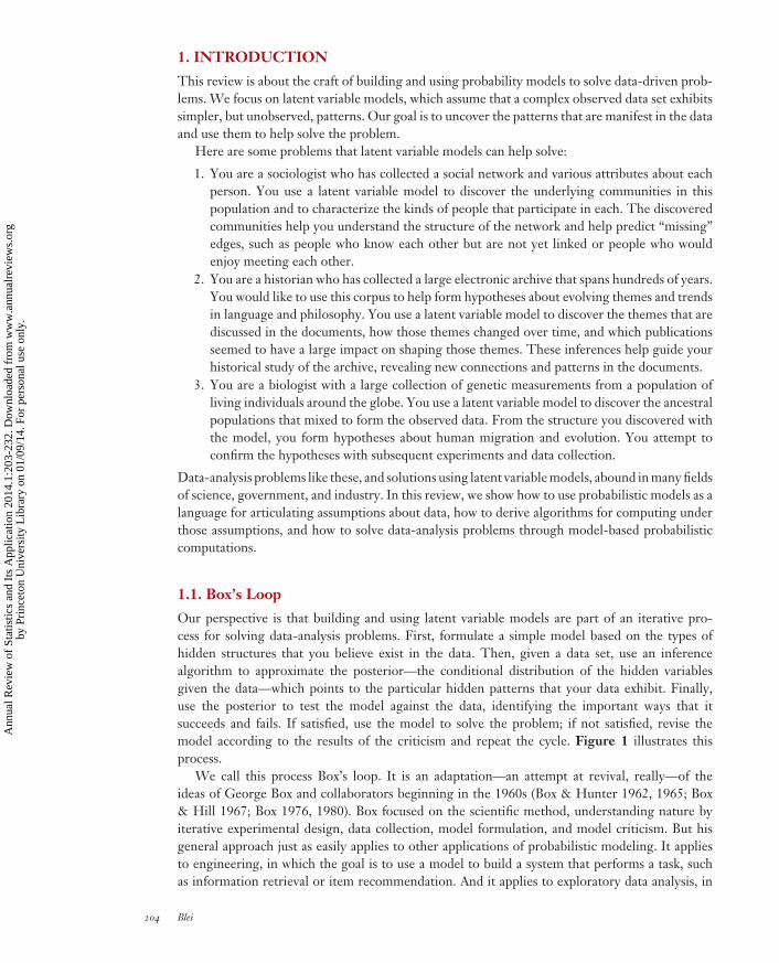
Our perspective is that building and using latent variable models are part of an iterative pro-cess for solving data-analysis problems. First, formulate a simple model based on the types ofhidden structures that you believe exist in the data. Then, given a data set, use an inferencealgorithm to approximate the posterior—the conditional distribution of the hidden variablesgiven the data—which points to the particular hidden patterns that your data exhibit. Finally,use the posterior to test the model against the data, identifying the important ways that itsucceeds and fails. If satisfied, use the model to solve the problem; if not satisfied, revise themodel according to the results of the criticism and repeat the cycle. Figure 1 illustrates thisprocess.
We call this process Box’s loop. It is an adaptation—an attempt at revival, really—of theideas of George Box and collaborators beginning in the 1960s (Box & Hunter 1962, 1965; Box& Hill 1967; Box 1976, 1980). Box focused on the scientific method, understanding nature byiterative experimental design, data collection, model formulation, and model criticism. But hisgeneral approach just as easily applies to other applications of probabilistic modeling. It appliesto engineering, in which the goal is to use a model to build a system that performs a task, suchas information retrieval or item recommendation. And it applies to exploratory data analysis, in
204 Blei
Ann
ual R
evie
w o
f St
atis
tics
and
Its
App
licat
ion
2014
.1:2
03-2
32. D
ownl
oade
d fr
om w
ww
.ann
ualr
evie
ws.
org
by P
rinc
eton
Uni
vers
ity L
ibra
ry o
n 01
/09/
14. F
or p
erso
nal u
se o
nly.

ST01CH10-Blei ARI 4 December 2013 17:0
Infer hidden quantitiesMarkov chain Monte Carlo,
variational inference,Laplace approximation
Criticize modelPerformance on a task,
prediction on unseen data,posterior predictive checks
Build modelMixtures and mixed-membership models,
time-series models, generalized linear models,factor models, Bayesian nonparametrics
REVISE MODEL
Apply modelPredictive systems,data exploration,
data summarization
DATA
Figure 1Box’s loop. Building and computing with models are part of an iterative process for solving data-analysis problems. This is Box’s loop, amodern interpretation of the perspective of Box (1976).
which the goal is to summarize, visualize, and hypothesize about observational data, namely datathat we observe but that are not part of a designed experiment.
Why revive this perspective now? The future of data analysis lies in close collaborationsbetween domain experts and modelers. Box’s loop cleanly separates the tasks of articulatingdomain assumptions into a probability model, conditioning on data and computing with thatmodel, evaluating it in realistic settings, and finally using the evaluation to revise the model’s as-sumptions. It is a powerful methodology for guiding collaborative efforts in solving data-analysisproblems.
As machine learning researchers and statisticians, our research goal is to make Box’s loopeasy to implement, and modern research has radically changed each component in the 50 yearssince Box’s original research. We have developed intuitive grammars for building models, scalablealgorithms for computing with a wide variety of models, and general methods for understandingthe performance of a model to guide its revision. This review provides a curated view of thestate-of-the-art research for implementing Box’s loop.
In the first step of the loop, we build (or revise) a probability model. The model itself is awell-defined mathematical object, but building a model is an art. For interesting perspectives,the reader is referred to Box & Draper (1987), Lehmann (1990), and Good [2009 (1983)]. Inthis review, we will draw on probabilistic graphical models (Pearl 1988, Dawid & Lauritzen1993, Jordan 2004), a field of research that connects graph theory to probability theory andprovides an elegant language for building models. With graphical models, we can clearly ar-ticulate what types of hidden structures are governing the data and construct complex modelsfrom simpler components—such as clusters, sequences, hierarchies, and others—to tailor ourmodels to the data at hand. This language gives us a palette with which to posit and revise ourmodels.
The observed data enter the picture in the second step of Box’s loop. Here, we compute theposterior distribution, the conditional distribution of the hidden patterns given the observations, to
www.annualreviews.org • Data Analysis with Latent Variable Models 205
Ann
ual R
evie
w o
f St
atis
tics
and
Its
App
licat
ion
2014
.1:2
03-2
32. D
ownl
oade
d fr
om w
ww
.ann
ualr
evie
ws.
org
by P
rinc
eton
Uni
vers
ity L
ibra
ry o
n 01
/09/
14. F
or p
erso
nal u
se o
nly.

ST01CH10-Blei ARI 4 December 2013 17:0
understand how the hidden structures we assumed are manifested in the data.1 Most useful modelsare difficult to compute with, however, and researchers have developed powerful approximateposterior inference algorithms for approximating these conditionals. Techniques such as Markovchain Monte Carlo (MCMC) (Metropolis et al. 1953, Hastings 1970, Geman & Geman 1984)and variational inference (Peterson & Anderson 1987, Jordan et al. 1999, Wainwright & Jordan2008) make it possible for us to examine large data sets with sophisticated statistical models.Moreover, these algorithms are modular—recurring components in a graphical model lead torecurring subroutines in their corresponding inference algorithms.
Finally, we close the loop, studying how our models succeed and fail to guide the process ofrevision. Here, again, is an opportunity for a revival. With new methods for quickly building andcomputing with sophisticated models, we can make better use of techniques such as predictivesample reuse (PSR) (Geisser 1975) and posterior predictive checks (PPCs) (Box 1980, Rubin1984, Meng 1994, Gelman et al. 1996). These techniques assess a model’s fitness by contrastingthe predictions that it makes against the observed data in the ways that matter to the task at hand.This activity, known as model criticism, is essential to solving modern data-analysis problems.
1.2. This Review
We describe each component of Box’s loop in turn. In Section 2, we describe probabilistic modelingas a language for expressing assumptions about data, and we provide graphical model notation asa convenient visual representation of structured probability distributions. In Section 3, we discussseveral simple examples of latent variable models and describe how they can be combined andexpanded when developing new models for new problems. In Section 4, we describe mean fieldvariational inference, a method of approximate posterior inference that can be easily applied to awide class of models and that can handle large data sets. Finally, in Section 5, we describe how tocriticize and assess the fitness of a model, using predictive likelihood and PPCs.
Again, this article represents a curated view. For other surveys of latent variable models, seeSkrondal & Rabe-Hesketh (2007), Ghahramani (2012), and Bishop (2013). For more completetreatments of probabilistic modeling, see books such as Bishop (2006) and Murphy (2013). Finally,for another perspective on iterative model building, see Krnjajic et al. (2008).
With the ideas presented here, our hope is that the reader can begin to iteratively build sophis-ticated methods to solve real-world problems. We emphasize, however, that data analysis withprobability models is a craft. Here, we survey some of its tools, but the reader will master themonly as with any other craft—with practice.
2. LATENT VARIABLE MODELS
When we build a latent variable model, we imagine what types of hidden quantities might be usedto describe the data we are interested in, and we encode that relationship in a joint probability dis-tribution of hidden and observed random variables. Then, given an observed data set, we uncoverthe particular hidden quantities that describe it through the posterior, which is the conditionaldistribution of the hidden variables given the observations. Furthermore, we use the posterior to
1In a way, we take a Bayesian perspective because we treat all hidden quantities as random variables and investigate themthrough their conditional distribution given observations. However, we prefer the more general language of latent variables,which can be either parameters to the whole data set or local hidden structure to individual data points (or something inbetween). Furthermore, in performing model criticism we will step out of the Bayesian framework to ask whether the modelwe assumed has good properties in the sampling sense.
206 Blei
Ann
ual R
evie
w o
f St
atis
tics
and
Its
App
licat
ion
2014
.1:2
03-2
32. D
ownl
oade
d fr
om w
ww
.ann
ualr
evie
ws.
org
by P
rinc
eton
Uni
vers
ity L
ibra
ry o
n 01
/09/
14. F
or p
erso
nal u
se o
nly.

ST01CH10-Blei ARI 4 December 2013 17:0
form the predictive distribution, the distribution over future data that the observations and themodel imply.
For example, the mixture model is one of the simplest latent variable models. A mixture modelassumes that the data are clustered and that each data point is drawn from a distribution associatedwith its assigned cluster. The hidden variables of the model are the cluster assignments andparameters to the per-cluster distributions. Given observed data, the mixture model posterioris a conditional distribution over clusterings and parameters. This conditional identifies a likelygrouping of the data and the characteristics of each group.
More formally, a model consists of three types of variables. The first type is an observation,which represents a data point. We denote N data points as x = x1:N . The second type is a hiddenvariable, which encodes hidden quantities (such as cluster memberships and cluster means) that areused to govern the distribution of the observations. We denote M hidden variables as h = h1:M .The third type is a hyperparameter, which is a fixed nonrandom quantity that we denote by η.Note that we focus on models of hidden and observed random variables, and we always assume thatthe hyperparameters are fixed. Estimating hyperparameters from data is the important problemof empirical Bayes (Efron & Morris 1973, Robbins 1980, Morris 1983, Efron 2013).
A model is a joint distribution of x and h, p(h, x | η) = p(h | η)p(x | h), which formally describeshow the hidden variables and observations interact in a probability distribution. After we observethe data, we are interested in the conditional distribution of the hidden variables, p(h | x, η) ∝p(h, x | η). The conditional distribution also leads to the predictive distribution, p(xnew | x) =∫
p(xnew | h)p(h | x, η)dh.We continue with the example of a Gaussian mixture model. The variables of the model are K
mixture components μ1:K , each of which is the mean of a Gaussian distribution, and a set of mixtureproportions θ , a nonnegative K vector that sums to one. Data arise by first choosing a componentassignment zn (an index from 1 to K) from the mixture proportions and then drawing the datapoint xn from the corresponding Gaussian: xi | zi ∼ N (μzi , 1). The hidden variables for this modelare the mixture assignments for each data point z1:N , the set of mixture component means μ1:K ,and the mixture proportions θ . To complete the model, we place distributions, known as priors,on the mixture components (e.g., a Gaussian) and the mixture proportions (e.g., a Dirichlet). Thefixed hyperparameters η are the parameters to these distributions.
Suppose we observe a data set x1:N of real values. We analyze these data with a Gaussian mixtureby estimating p(μ1:K , θ, z1:N | x1:N ), the posterior distribution of the mixture components, themixture proportions, and the way the data are clustered. This posterior reveals hidden structurein our data—it clusters the data points into K groups and describes the location (i.e., the mean)of each group.2 The predictive distribution, derived from the posterior, provides the distributionof the next data point. Figure 2 shows an example. Below, we describe three ways of specifying amodel: its generative probabilistic process, its joint distribution, and its directed graphical model.
2.1. The Generative Probabilistic Process
The generative probabilistic process describes how data would arise from the model. Though themodel is rarely “true,” the generative process helps make clear how the latent variables interact
2Note, however, that even after computing the posterior, we do not yet know that a Gaussian mixture is a good modelfor our data. No matter which data we observe, we can obtain a posterior over the hidden variables, that is, a clustering.(Furthermore, note that the number of mixture components is fixed—the number we chose may not be appropriate.) Afterwe have formulated the model and inferred the posterior, we discuss in Section 5 how to check whether it adequately explainsthe data.
www.annualreviews.org • Data Analysis with Latent Variable Models 207
Ann
ual R
evie
w o
f St
atis
tics
and
Its
App
licat
ion
2014
.1:2
03-2
32. D
ownl
oade
d fr
om w
ww
.ann
ualr
evie
ws.
org
by P
rinc
eton
Uni
vers
ity L
ibra
ry o
n 01
/09/
14. F
or p
erso
nal u
se o
nly.

ST01CH10-Blei ARI 4 December 2013 17:0
−2.5
0.0
2.5
5.0
−6 −4 −2x
y
a
−2.5
0.0
2.5
5.0
−6 −4 −2x
y
b
Figure 2Example data and inference with a mixture of Gaussians. (a) A data set of 100 points. (b) The same data set, now visualized with thehidden structure that we derived from approximating the posterior for a mixture of four Gaussians. Each data point is colored with itsmost likely assigned cluster, the most likely cluster means are marked in gray, and the contours give the posterior predictive distributionof the next data point.
to govern the distribution of the observations. The generative process for the Gaussian mixturemodel is the following:
1. Draw mixture proportions θ ∼ Dirichlet(α).2. For each mixture component k, draw μk ∼ N (0, σ 2
0 ).3. For each data point n:
a. Draw mixture assignment zn| θ ∼ Discrete(θ ).b. Draw data point xn| zn, μ ∼ N (μzn , 1).
The posterior distribution can be considered to reverse this process: Given data, what is thedistribution of the hidden structure that probably generated them?
This process makes the hyperparameters explicit; they are the variance of the prior on themixture components σ 2
0 and the Dirichlet3 parameters α. The process also helps us identify localand global hidden variables. The global variables are the mixture proportions θ and the mixturecomponents μ = μ1:K . These variables describe hidden structure that is shared for the entire dataset. The local variables are the mixture assignments; each assignment zi helps govern only thedistribution of the ith observation. This distinction becomes important in Section 4, when wediscuss algorithms for approximating the posterior.
2.2. The Joint Distribution
The traditional way of representing a model is with the factored joint distribution of its hiddenand observed variables. This factorization comes directly from the generative process. For the
3The Dirichlet distribution is a distribution on the simplex, nonnegative vectors that sum to one. Thus, a draw from a Dirichletcan be used as a parameter to a multinomial downstream in the model. Furthermore, note that we refer to a single draw froma multinomial (or a multinomial with N = 1) as a discrete distribution.
208 Blei
Ann
ual R
evie
w o
f St
atis
tics
and
Its
App
licat
ion
2014
.1:2
03-2
32. D
ownl
oade
d fr
om w
ww
.ann
ualr
evie
ws.
org
by P
rinc
eton
Uni
vers
ity L
ibra
ry o
n 01
/09/
14. F
or p
erso
nal u
se o
nly.

ST01CH10-Blei ARI 4 December 2013 17:0
Gaussian mixture, the joint is
p(θ, μ, z, x | σ 20 , α) = p(θ | α)
K∏k=1
p(μk | σ 20 )
N∏i=1
(p(zi | θ )p(xi | zi , μ)). 1.
For each term, we substitute the appropriate density function. In this case, p(θ |α) is the Dirichletdensity, p(μk | σ0) is the Gaussian density, p(zi | θ ) = θzi is a discrete distribution, and p(xi | zi , μ)is a Gaussian density centered at the zith mean. Notice the distinction between local and globalvariables: Local variables have terms inside the product over N data points, whereas global variableshave terms outside of this product.
The joint distribution lets us calculate the posterior. In the Gaussian mixture model, theposterior is
p(θ, μ, z | x, σ 20 , α) = p(θ, μ, z, x | σ 2
0 , α)p(x | σ 2
0 , α). 2.
We use the posterior to examine the particular hidden structure that is manifest in the observeddata. We also use the posterior (over the global variables) to form the posterior predictive distri-bution of future data. For the mixture, the predictive distribution is
p(xnew | x, σ 20 , α) =
∫ (∑znew
p(znew | θ )p(xnew | znew, μ, σ 20 )
)p(θ, μ | x, σ 2
0 , α)dθdμ. 3.
The inner sum marginalizes out the local hidden variables for the new data point, conditionedon the global hidden variables. The outer integral marginalizes out the global hidden variables,conditioned on the data. In Section 5, we discuss how the predictive distribution is important forchecking and criticizing latent variable models.
The denominator of Equation 2 is the marginal probability of the data, also known as theevidence, which is found by marginalizing out the hidden variables from the joint. For manyinteresting models, the evidence is difficult to efficiently compute, and developing approximationsto the posterior has thus been a focus of modern Bayesian statistics. In Section 4, we describevariational inference, a technique for approximating the posterior that emerged from the statisticalmachine learning community.
2.3. The Graphical Model
Our final way of viewing a latent variable model is as a probabilistic graphical model, an-other representation that derives from the generative process. The generative process indicatesa pattern of dependence among the random variables. For example, in the mixture model’sprocess, the mixture components μk and mixture proportions θ do not depend on any hid-den variables; they are generated from distributions parameterized by fixed hyperparameters(steps 1 and 2 in the generative process described in Section 2.1). The mixture assignment zi
depends on the mixture proportions θ , which parameterizes its distribution (step 3a). The ob-servation xi depends on the mixture components μ and mixture assignment zi (step 3b). Wecan encode these dependencies with a graph in which nodes represent random variables andedges denote dependence between them. This is a graphical model.4 The graphical modelillustrates the structure of the factorized joint distribution and the flow of the generativeprocess.
4Formally, the semantics of graphical models assert that there is a possible dependence between random variables connectedby an edge. Here, as a practical matter, we read the graph as asserting dependence.
www.annualreviews.org • Data Analysis with Latent Variable Models 209
Ann
ual R
evie
w o
f St
atis
tics
and
Its
App
licat
ion
2014
.1:2
03-2
32. D
ownl
oade
d fr
om w
ww
.ann
ualr
evie
ws.
org
by P
rinc
eton
Uni
vers
ity L
ibra
ry o
n 01
/09/
14. F
or p
erso
nal u
se o
nly.

ST01CH10-Blei ARI 4 December 2013 17:0
α
x1 x2 x3
z1 z2 z3
σ0
θ
μ1 μ2
σ0
K
N
zn
xn
α
~ DirichletK(α)
~ Discrete(θ)
θ
μk
a b
Figure 3(a) A graphical model for a mixture of two Gaussians. There are three data points. The shaded nodes areobserved variables, the unshaded nodes are hidden variables, and the blue square boxes are fixedhyperparameters (such as the Dirichlet parameters). (b) A graphical model for a mixture of K Gaussians withN data points.
Figure 3a illustrates a graphical model for three data points drawn from a mixture of twoGaussians. This is an unpacked model, in which each data point is given its own substructure inthe graph. We can summarize repeated components of a model with plates, rectangles that encasea substructure to denote replication. Figure 3b is a more succinct graphical model for N datapoints modeled with a mixture of K Gaussians.
The field of graphical models provides a powerful approach to reasoning about probabilitydistributions. It connects the topological structure of a graph with elegant algorithms for comput-ing various quantities about the joint distributions that the graph describes. Formally, a graphicalmodel represents the family of distributions that respects the independencies it implies. (Theseinclude the basic independencies described above, along with others that derive from graph the-oretic calculations.) We do not discuss graphical models in depth. Good references include Pearl(1988), Jordan (1999), Bishop (2006), Koller & Friedman (2009), and Murphy (2013).
We simply use graphical models as a convenient visual language for expressing how hiddenstructure interacts with observations. In our applied research, we have found that graphical modelsare useful for domain experts (such as scientists) to build and discuss models with statisticians andcomputer scientists.
3. EXAMPLE MODELS
Above, we describe the basic idea behind latent variable models and provide a simple example, theGaussian mixture model. In this section, we describe some of the commonly recurring componentsin latent variable models—mixed memberships, linear factors, matrix factors, and time series—andpoint to some of their applications.
Many of the models we describe below were discovered (and sometimes rediscovered) in specificresearch communities. They were often bundled with a particular algorithm for carrying outposterior inference and were sometimes developed without a probabilistic modeling perspective.
210 Blei
Ann
ual R
evie
w o
f St
atis
tics
and
Its
App
licat
ion
2014
.1:2
03-2
32. D
ownl
oade
d fr
om w
ww
.ann
ualr
evie
ws.
org
by P
rinc
eton
Uni
vers
ity L
ibra
ry o
n 01
/09/
14. F
or p
erso
nal u
se o
nly.

ST01CH10-Blei ARI 4 December 2013 17:0
Here, we present these models probabilistically and treat them more generally than as stand-alone solutions. We separate the independence assumptions they make from their distributionalassumptions, and we postpone until Section 4 our discussion of how to compute the posterior.
The models below are useful in and of themselves—we select a set of models that have use-ful applications and a history in the statistics and machine learning literature—but we hope todeemphasize their role in a “cookbook” of methods. Rather, we highlight their use as compo-nents in more complex models for more complex problems and data. This is the advantage of theprobabilistic modeling framework.
3.1. Linear Factor Models
Linear factor models embed high-dimensional observed data in a low-dimensional space. Thesemodels have been a mainstay in the field of statistics for nearly a century; principal componentanalysis (Pearson 1901, Hotelling 1933), factor analysis (Thurstone 1931, 1938; Thomson 1939),and canonical correlation analysis (Hotelling 1936) can all be interpreted this way, althoughthe probabilistic perspective on them is more recent (Roweis 1998, Tipping & Bishop 1999,Collins et al. 2002). Factor models are important as a component in more complicated models(such as the Kalman filter; see Section 3.4.2. below) and have generally spawned many extensions(Bartholomew et al. 2011).
In a factor model, there is a set of hidden components, and each data point is associated with ahidden vector of weights, with one weight for each component. The data arise from a distributionwhose parameters combine the global components with the per–data point weights. Conditionedon data, the posterior locates the global components that describe the data set and the local weightsfor each data point. The components capture general patterns in the data; the weights capturehow each data point exhibits those patterns and serve as a low-dimensional embedding of thehigh-dimensional data.
Figure 4a illustrates the graphical model. Notice that the independence assumptions about thehidden and observed variables (which come from the structure of the graphical model) are similarto those from the mixture model (Figure 3). Suppose the data are p-dimensional. The linear factormodel contains K components μ1:K , each of which is a p-vector. We organize the componentsinto a K × p matrix μ. For each data point n, we draw a K-dimensional weight vector wn andthen draw the data point from a distribution parameterized by w�
n μ. Traditionally, the data aredrawn from a Gaussian (Tipping & Bishop 1999), but extensions to linear factors have consideredexponential families in which w�
n μ is the natural parameter (Collins et al. 2002, Mohamed et al.2008).
3.2. Mixed-Membership Models
Mixed-membership models are used for unsupervised analyses of grouped data, multiple sets ofobservations that we assume are statistically related to each other. In a mixed-membership model,each group is drawn from a mixture, in which the mixture proportions are unique to the groupand the mixture components are shared across groups.
Consider the following examples: Text data are collections of documents, each containing aset of observed words; genetic data are collections of people, each containing observed allelesat various locations along the genome; survey data are completed surveys, each a collection ofanswers by a single respondent; social networks are collections of people, each containing a set ofconnections to others. In these settings, mixed-membership models assume that there is a singleset of coherent patterns underlying the data—themes in text (Blei et al. 2003), populations in
www.annualreviews.org • Data Analysis with Latent Variable Models 211
Ann
ual R
evie
w o
f St
atis
tics
and
Its
App
licat
ion
2014
.1:2
03-2
32. D
ownl
oade
d fr
om w
ww
.ann
ualr
evie
ws.
org
by P
rinc
eton
Uni
vers
ity L
ibra
ry o
n 01
/09/
14. F
or p
erso
nal u
se o
nly.

ST01CH10-Blei ARI 4 December 2013 17:0
K
K
zt ~ Discrete(θzt–1)
~ θkDirichletK(α)
xt ~ p( ·|μzt)
μk ~ p( ·|η)μk
α
xt–1 xt xt+1
zt–1 zt zt+1
η
θk
d Hidden Markov model
K
xt ~ p( ·|wtTμ)
μk
xt–1 xt xt+1
wt–1 wt wt+1
σμ
θw
e Kalman filter
η
K
NM
xmn
~ Discrete(θm)
~ DirichletK(α)
~ p( ·|μznm)
~ p( ·|η)μk
zmn
θm
α
~ p( ·|wnTμ)
σμ
K
N
wn
xn
μk
σw
a Linear factor b Mixed membership
σγ
M
N
wn
xmn ~ p( ·|wnTγm)
γm
σw
c Matrix factorization
Figure 4Graphical models for the model components described in Section 3. (a) Linear factor model. (b) Mixed-membership model. (c) Matrixfactorization. (d ) Hidden Markov model. (e) Kalman filter.
genetic data (Pritchard et al. 2000), types of respondents in survey data (Erosheva et al. 2007), andcommunities in networks (Airoldi et al. 2008)—but that each group exhibits a different subset ofthose patterns and to different degrees.
Mixed-membership models posit a set of global mixture components. Each data group ariseswhen we first choose a set of mixture proportions and then, for each observation in the group,choose a mixture assignment from the per-group proportions and the data point from its cor-responding component. The groups share the same set of components, but each exhibits themwith a different proportion. Thus, the mixed-membership posterior uncovers the recurring pat-terns in the data and the proportion with which they occur in each group. Contrast this situation
212 Blei
Ann
ual R
evie
w o
f St
atis
tics
and
Its
App
licat
ion
2014
.1:2
03-2
32. D
ownl
oade
d fr
om w
ww
.ann
ualr
evie
ws.
org
by P
rinc
eton
Uni
vers
ity L
ibra
ry o
n 01
/09/
14. F
or p
erso
nal u
se o
nly.

ST01CH10-Blei ARI 4 December 2013 17:0
with that of simple mixture models, in which each data group is associated with a single mixturecomponent. Mixed-membership models give better predictions than do mixture models and pro-vide more interesting exploratory structure.
Figure 4b illustrates the graphical model for a mixed-membership model. There are M groupsof N data points; the observation xmn is the nth observation in the mth group.5 The hidden variableμk is an appropriate parameter to a distribution of xmn (e.g., if the observation is discrete, then μk
is a discrete distribution), and p(· | η) is an appropriate prior with hyperparameter η. The otherhidden variables are per-group mixture proportions θm, a point on the simplex (i.e., K vectorsthat are positive and sum to one), and per-observation mixture assignments zmn, each of whichindexes one of the components. Given grouped data, the posterior finds the mixture componentsthat describe the whole data set and mixture proportions for each group. Note that the mixturegraphical model of Figure 3 is a component of this more complicated model.
For example, mixed-membership models of documents—in which each document is a groupof observed words—are known as topic models (Blei et al. 2003, Erosheva et al. 2004, Steyvers& Griffiths 2006, Blei 2012). In a topic model, the data-generating components are probabilitydistributions over a vocabulary, and each document is modeled as a mixture of these distributions.Given a collection, the posterior components place their probability mass on terms that are associ-ated under a single theme—which connects to words that tend to co-occur—and thus are termedtopics. The posterior proportions indicate how each document exhibits those topics; for example,one document might be about “sports” and “health,” whereas another may be about “sports” and“business.” (Again, we emphasize that the topics too are uncovered by the posterior.) Figure 5shows the topics from a topic model fit to 1.8 million articles from the New York Times. This figurewas made by estimating the posterior (Section 4) and then plotting the most frequent words fromeach topic.
3.3. Matrix Factorization Models
Many data sets are organized into a matrix, in which each observation is indexed by a row and acolumn. Our goal may be to understand something about the rows and columns, or to predict thevalues of unobserved cells. For example, in the Netflix challenge problem (Bell & Koren 2007),we observe a matrix in which rows are users, columns are movies, and each cell xnm (if observed)is how user n rated movie m. The goal is to predict which movies user n will like that she has notyet seen. Another example is political roll-call data: how lawmakers vote on proposed bills. In theroll-call matrix, rows are lawmakers, columns are bills, and each cell is how lawmaker n voted onbill m. Here, the main statistical problem involves exploration. Where do the lawmakers sit onthe political spectrum? Which ones are most conservative? Which ones are most liberal?
A matrix factorization model uses hidden variables to embed both the rows and the columns ina low-dimensional space. Each observed cell is modeled by a distribution whose parameters are alinear combination of the row embedding and column embedding; for example, cells in a single rowshare the same row embedding but are governed by different column embeddings. Conditionedon an observed matrix, the posterior distribution provides low-dimensional representations of itsrows and columns. These representations can be used to form predictions about unseen cells andto explore hidden structure in the data.
For example, in the movie recommendation problem we use the model to cast each user andmovie in a low-dimensional space. For an unseen cell (a particular user who has not watched
5Each group need not have the same number of observations, but this makes the notation cleaner.
www.annualreviews.org • Data Analysis with Latent Variable Models 213
Ann
ual R
evie
w o
f St
atis
tics
and
Its
App
licat
ion
2014
.1:2
03-2
32. D
ownl
oade
d fr
om w
ww
.ann
ualr
evie
ws.
org
by P
rinc
eton
Uni
vers
ity L
ibra
ry o
n 01
/09/
14. F
or p
erso
nal u
se o
nly.

ST01CH10-Blei ARI 4 December 2013 17:0
Game
Second
SeasonTeam
Play
Games
Players
Points
Coach
Giants
1
House
Bush
Political
Party
ClintonCampaign
Republican
Democratic
SenatorDemocrats
6
School
Life
Children
Family
Says
Women
HelpMother
ParentsChild
11
StreetSchool
House
Life
Children
FamilySays
Night
Man
Know
2
Percent
Street
House
Building
Real
SpaceDevelopment
SquareHousing
Buildings
7
Percent
Business
Market
Companies
Stock
Bank
Financial
Fund
InvestorsFunds
12
Life
Says
Show
ManDirector
Television
Film
Story
Movie
Films
3
Game
SecondTeam
Play
Won
Open
Race
Win
RoundCup
8
Government
Life
WarWomen
PoliticalBlack
Church
Jewish
Catholic
Pope
13
House
Life
Children
Man
War
Book
Story
Books
Author
Novel
4
Game
Season
Team
RunLeague
GamesHit
Baseball
Yankees
Mets
9
Street
Show
ArtMuseum
WorksArtists
Artist
Gallery
ExhibitionPaintings
14
Street
House
NightPlace
Park
Room
Hotel
Restaurant
Garden
Wine
5
Government
Officials
WarMilitary
Iraq
Army
Forces
Troops
Iraqi
Soldiers
10
Street
YesterdayPolice
Man
CaseFound
Officer
Shot
Officers
Charged
15
Figure 5Topics found in a corpus of 1.8 million articles from the New York Times. Modified from Hoffman et al. (2013).
a particular movie), our prediction of the rating depends on a linear combination of the user’sembedding and the movie’s embedding. We can also use these inferred representations to findgroups of users that have similar tastes and groups of movies that are enjoyed by the same kindsof users.
Figure 4c illustrates the graphical model. This model is closely related to a linear factor model,except that each cell’s distribution is determined by hidden variables that depend on the cell’s rowand column. The overlapping plates show how the observations at the nth row share its embeddingwn but use different variables γm for each column. Similarly, the observations in the mth columnshare its embedding γm but use different variables wn for each row. Casting matrix factorization
214 Blei
Ann
ual R
evie
w o
f St
atis
tics
and
Its
App
licat
ion
2014
.1:2
03-2
32. D
ownl
oade
d fr
om w
ww
.ann
ualr
evie
ws.
org
by P
rinc
eton
Uni
vers
ity L
ibra
ry o
n 01
/09/
14. F
or p
erso
nal u
se o
nly.

ST01CH10-Blei ARI 4 December 2013 17:0
−2 0 2 4
Robert Berry
Eric Canto
r
Jesse
Jack
son
Timoth
y Johnso
n
Dennis Kucin
ich
James M
arshall
Ronald Paul
Michael M
cCaul
Harry M
itchell
Anh Cao
Figure 6Ideal point models separate Republicans (red ) from Democrats (blue) and try to capture the degree to which each lawmaker is liberal orconservative. Modified courtesy of Sean Gerrish.
as a general probabilistic model is known as probabilistic matrix factorization (Salakhutdinov &Mnih 2008).
Matrix factorization is widely used. In quantitative political science, ideal point models areone-dimensional matrix factorizations of legislative roll-call data (Clinton et al. 2004). Figure 6illustrates the one-dimensional embeddings of lawmakers in the one hundred fifteenth USCongress. The model captured the divide between Democrats and Republicans and identifieda finer-grained political spectrum from liberal to conservative. Similar models are used in edu-cational testing scenarios, in which rows are testers and columns are questions on a test (Baker1992). Finally, extensions of matrix factorization models were important in winning the Netflixchallenge (Koren et al. 2009). The developers of the winning approach essentially took into ac-count Box’s loop; they fitted simple matrix models first and then, as a result of insightful modelcriticism, embellished the basic model to consider important elements such as time and (latent)movie popularity.
3.4. Time-Series Models
Many observations are sequential: They are indexed by time or position, and we want to take thisstructure into account when making inferences. For example, genetic data are indexed by locationon the chromosome; data from radar observations are indexed by time; words in a sentence areindexed by their position. There are two canonical and closely related latent variable models of timeseries: the hidden Markov model (HMM) and the Kalman filter. Each has had important scientificand engineering applications, and each demonstrates how we can use simple latent variable modelsto construct more complex ones.
3.4.1. Hidden Markov models. In an HMM, each observation of the time series is drawn froman unobserved mixture component, and that component is drawn conditional on the previousobservation’s mixture component. The posterior is similar to a mixture model, but one in whichthe model assumes a Markovian structure on the sequence of mixture assignments. HMMs havebeen successfully used in many applications, notably in speech recognition (Rabiner 1989) andcomputational biology (Durbin et al. 1998). For example, in speech recognition, the hidden statesrepresent words from a vocabulary, the Markov process is a model of natural language (whichmay be more complex than the simple first-order model described above), and the data are theobserved audio signal. Posterior inference of the hidden states provides an estimate of what isbeing said in the audio signal.
Figure 4d illustrates the graphical model; note how modeling a time series translates to alinked chain in the graph. The global hidden variables are the mixture components μ1:K (as in amixture model or a mixed-membership model) and the transition probabilities θ1:K . The transition
www.annualreviews.org • Data Analysis with Latent Variable Models 215
Ann
ual R
evie
w o
f St
atis
tics
and
Its
App
licat
ion
2014
.1:2
03-2
32. D
ownl
oade
d fr
om w
ww
.ann
ualr
evie
ws.
org
by P
rinc
eton
Uni
vers
ity L
ibra
ry o
n 01
/09/
14. F
or p
erso
nal u
se o
nly.

ST01CH10-Blei ARI 4 December 2013 17:0
probabilities provide K conditional distributions over the next component, given the value of theprevious one.
3.4.2. The Kalman filter. Whereas an HMM is a time-series adaptation of the mixture model,a Kalman filter is a time-series adaptation of a linear (Gaussian) factor model (Kalman 1960). Inparticular, we draw the row embeddings from a state-space model, a Gaussian whose mean is theprevious position’s embedding. See West & Harrison (1997) for a general probabilistic perspectiveon continuous time series.
Kalman filters are influential in radar tracking applications, in which wt is a vector that repre-sents the latent position of an object in space, the state-space model captures the assumed processby which the position moves (which may be more complex than the simple process laid out above),and the observations represent blips on a radar screen that are corrupted by noise (Bar-Shalomet al. 2004). Inferences from this model help track an object’s true position and predict its nextposition.
Figure 4e illustrates the graphical model. Although the underlying distributions are different—in the Kalman filter the hidden chain of variables is a sequence of continuous variables, rather thandiscrete ones—the structure of the graphical model is nearly the same as for the HMM. Althoughthe algorithms for the HMM and the Kalman filter were developed independently for differentpurposes and in different research communities, they are both instances of general algorithmsfor graphical models. Finding such connections, and developing diverse applications with newmodels, is one of the advantages of the graphical model formalism.
3.5. The Craft of Latent Variable Modeling
Above, we describe a selection of latent variable models, each of which builds on simpler models.However, we emphasize that our goal is not to deliver a complete catalog of models. In fact, weomit some important types of models, such as Bayesian nonparametric models (Ferguson 1973,Antoniak 1974, Teh & Jordan 2008, Hjort et al. 2010, Gershman & Blei 2012) that let the datadetermine the structure of the latent variables, random effects models (Gelman et al. 1995) thatallow data to depend on hidden covariates, and hierarchical models (Gelman & Hill 2007) thatallow data to exhibit complex and overlapping groups. Rather, we want to demonstrate how touse probability modeling as a language of assumptions for tailoring latent variable models to eachdata-analysis challenge.
There are several ways to adapt and develop new latent variable models. One way to adapt amodel is to change the data-generating distribution of an existing model. At the bottom of eachprobabilistic process is a step that generates an observation conditioned on the latent structure.For example, in the mixed-membership model, the observation is drawn from a distributionconditioned on a component; in the factor model, it is a distribution conditioned on a linearcombination of weights and factors. Depending on the type of observation at hand, changing thisdistribution can lead to new latent variable models. We might use ordinal distributions for ordereddata, gamma distributions and truncated Gaussians for positive data, or discrete distributions forcategorical data. We can even use conditional models, such as generalized linear models (Nelder& Wedderburn 1972, McCullagh & Nelder 1989), that use observed (but not modeled) covariatesto help describe the data distribution.
Another way to develop new models is to change the distributional assumptions on the latentvariables. We might replace a Gaussian with a gamma distribution to enforce positivity. Doingso fundamentally changes models such as Gaussian matrix factorization to a form of nonnegativematrix factorization, a technique that is important in computer vision problems (Lee & Seung
216 Blei
Ann
ual R
evie
w o
f St
atis
tics
and
Its
App
licat
ion
2014
.1:2
03-2
32. D
ownl
oade
d fr
om w
ww
.ann
ualr
evie
ws.
org
by P
rinc
eton
Uni
vers
ity L
ibra
ry o
n 01
/09/
14. F
or p
erso
nal u
se o
nly.

ST01CH10-Blei ARI 4 December 2013 17:0
1880Electric
MachinePowerEngineSteam
TwoMachines
IronBattery
Wire
1890ElectricPower
CompanySteam
ElectricalMachine
TwoSystemMotor
Engine
1900Apparatus
SteamPowerEngine
EngineeringWater
ConstructionEngineer
RoomFeet
1910Air
WaterEngineeringApparatus
RoomLaboratoryEngineer
MadeGas
Tube
1920Apparatus
TubeAir
PressureWaterGlassGas
MadeLaboratory
Mercury
1930Tube
ApparatusGlass
AirMercury
LaboratoryPressure
MadeGas
Small
Air
1940
TubeApparatus
GlassLaboratory
RubberPressure
SmallMercury
Gas
1950Tube
ApparatusGlass
AirChamber
InstrumentSmall
LaboratoryPressureRubber
1960Tube
SystemTemperature
AirHeat
ChamberPowerHigh
InstrumentControl
1970Air
HeatPowerSystem
TemperatureChamber
HighFlowTube
Design
1980High
PowerDesign
HeatSystemSystemsDevices
InstrumentsControlLarge
1990Materials
HighPower
CurrentApplicationsTechnology
DevicesDesignDeviceHeat
2000DevicesDevice
MaterialsCurrent
GateHighLight
SiliconMaterial
Technology
Figure 7A dynamic topic found with a dynamic topic model applied to a large corpus from the magazine Science. The model has captured theidea of technology and how it has changed throughout the course of the collection. Modified from Blei (2012).
1999). Alternatively, we might replace simple distributions with more complex distributions thatthemselves have latent structure. For example, the idea behind so-called spike and slab modeling(Ishwaran & Rao 2005) is to generate a vector (such as the hidden weights in a factor model) in atwo-stage process: First, generate a bank of binary variables that indicate which factors are relevantto a data point, and second, generate the weights of those factors from an appropriate distribution.This process provides a sparse hidden vector in a way that a simple distribution cannot.
Finally, we can mix and match components from different models to create wholly new tech-niques. For example, a dynamic topic model captures documents that are organized in time (Blei& Lafferty 2006). At each time point, the documents are modeled with a mixed-membershipmodel, but the components are connected sequentially from time point to time point. Figure 7illustrates one of the topic sequences found with a dynamic topic model fit to the magazine Science.Incorporating time gives a much richer latent structure than we find with the model of Figure 5.Dynamic topic models take elements from mixed-membership models and Kalman filters to solvea unique problem—they find the themes that underlie the collection and reveal how those themeschange smoothly through time.
As another example, McAuliffe et al. (2004) and Siepel & Haussler (2004) combined tree-basedmodels and HMMs to simultaneously analyze genetic data from a collection of species organizedin a phylogenetic tree. These models can predict the exact locations of protein-coding genescommon to all the species in the collection.
www.annualreviews.org • Data Analysis with Latent Variable Models 217
Ann
ual R
evie
w o
f St
atis
tics
and
Its
App
licat
ion
2014
.1:2
03-2
32. D
ownl
oade
d fr
om w
ww
.ann
ualr
evie
ws.
org
by P
rinc
eton
Uni
vers
ity L
ibra
ry o
n 01
/09/
14. F
or p
erso
nal u
se o
nly.

ST01CH10-Blei ARI 4 December 2013 17:0
We emphasize that we have only scratched the surface of the types of models that we canbuild. Models can be formed from myriad components—binary vectors, time series, hierarchies,mixtures—which can be composed and connected in many ways. With practice and experience inprobabilistic models, data analysts are able to both formally express the type of latent structurethey want to uncover and devise the generative assumptions that can capture it.
4. POSTERIOR INFERENCE WITH MEAN FIELDVARIATIONAL METHODS
In Sections 2 and 3, we describe the probabilistic modeling formalism, discuss several latent vari-able models, and show how they can be combined and expanded to create new models. We nowturn to the nuts and bolts of how to use models with observed data—how to uncover hidden struc-ture and how to form predictions about new data. Both problems hinge on computing the posteriordistribution, the conditional distribution of the hidden variables given the observations. Comput-ing or approximating the posterior is the central algorithmic problem in probabilistic modeling.(It is the second step of Box’s loop in Figure 1.) This is the problem of posterior inference.
For some basic models we can compute the posterior exactly, but for most interesting modelswe must approximate it, and researchers in Bayesian statistics and machine learning have pioneeredmany methods for approximate inference. The most widely used methods include Laplace approx-imations and Markov chain Monte Carlo (MCMC) sampling. Laplace approximations (Tierneyet al. 1989) represent the posterior as a Gaussian, derived from a Taylor approximation. Laplaceapproximations work well in some simple models but are difficult to use in high-dimensional set-tings (MacKay 2003). The reader is referred to Smola et al. (2003) and Rue et al. (2009) for recentinnovations.
MCMC sampling methods (Robert & Casella 2004) include fundamental algorithms suchas Metropolis–Hastings (Metropolis et al. 1953, Hastings 1970) and Gibbs sampling (Geman& Geman 1984, Gelfand & Smith 1990). Such methods form a Markov chain over the hiddenvariables whose stationary distribution is the posterior of interest. The algorithm simulates thechain, drawing consecutive samples from its transition distribution, to collect independent samplesfrom its stationary distribution. It approximates the posterior with the empirical distribution overthose samples. MCMC is a workhorse of modern Bayesian statistics.
Approximate posterior inference is an active field, and it is not our purpose to survey its manybranches. Rather, we discuss a particular strategy, mean field variational inference. Variationalinference is a deterministic alternative to MCMC in which sampling is replaced by optimization( Jordan et al. 1999, Wainwright & Jordan 2008). In practice, variational inference tends to befaster than sampling methods, especially with large and high-dimensional data sets, but it hasbeen less vigorously studied in the statistics literature. Using stochastic optimization (Robbins &Monro 1951), variational inference scales to massive data sets (Hoffman et al. 2013).
In this section, we first describe conditionally conjugate models, a large subclass of latentvariable models. Then we present the simplest variational inference algorithm, mean field infer-ence, for this subclass. Mean field variational inference provides a generic way to approximate theposterior for many models.6
6This section is more mathematically dense and abstract than the rest of this review. Readers may want to skip it if they arecomfortable approximating a posterior with a different method (and not interested in reading about variational inference) orknow someone who will implement posterior inference programs for their models and do not need to absorb the details.
218 Blei
Ann
ual R
evie
w o
f St
atis
tics
and
Its
App
licat
ion
2014
.1:2
03-2
32. D
ownl
oade
d fr
om w
ww
.ann
ualr
evie
ws.
org
by P
rinc
eton
Uni
vers
ity L
ibra
ry o
n 01
/09/
14. F
or p
erso
nal u
se o
nly.
ST01CH10-Blei ARI 4 December 2013 17:0
KL divergence
Latent variable model Variational family
N
η
zn xn
β
N
λ
ϕn zn
β
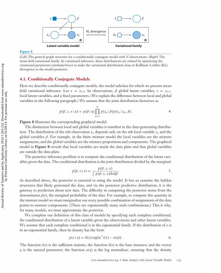
Figure 8(Left) The general graph structure for a conditionally conjugate model with N observations. (Right) Themean field variational family. In variational inference, these distributions are related by optimizing thevariational parameters (unshaded boxes) to make the variational distribution close in Kullback–Leibler (KL)divergence to the model posterior.
4.1. Conditionally Conjugate Models
Here we describe conditionally conjugate models, the model subclass for which we present meanfield variational inference. Let x = x1:N be observations, β global latent variables, z = z1:N
local latent variables, and η fixed parameters. (We explain the difference between local and globalvariables in the following paragraph.) We assume that the joint distribution factorizes as
p(β, z, x | η) = p(β | η)N∏
n=1
p(zn | β)p(xn | zn, β). 4.
Figure 8 illustrates the corresponding graphical model.The distinction between local and global variables is manifest in the data-generating distribu-
tion. The distribution of the nth observation xn depends only on the nth local variable zn and theglobal variables β. For example, in the finite mixture model the local variables are the mixtureassignments, and the global variables are the mixture proportions and components. The graphicalmodel in Figure 8 reveals that local variables are inside the data plate and that global variablesare outside the data plate.
The posterior inference problem is to compute the conditional distribution of the latent vari-ables given the data. The conditional distribution is the joint distribution divided by the marginal:
p(β, z | x) = p(β, z, x)∫p(β, z, x)dzdβ
. 5.
As described above, the posterior is essential to using the model. It lets us examine the hiddenstructures that likely generated the data, and via the posterior predictive distribution, it is thegateway to prediction about new data. The difficulty in computing the posterior stems from thedenominator p(x), the marginal probability of the data. For example, to compute this quantity inthe mixture model we must marginalize out every possible combination of assignments of the datapoints to mixture components. (There are exponentially many such combinations.) This is why,for many models, we must approximate the posterior.
We complete our definition of this class of models by specifying each complete conditional,the conditional distribution of a latent variable given the observations and other latent variables.We assume that each complete conditional is in the exponential family. If the distribution of x isin an exponential family, then its density has the form
p(x | η) = h(x) exp{η�t(x) − a(η)}. 6.
The function t(x) is the sufficient statistic; the function h(x) is the base measure; and the vectorη is the natural parameter; the function a(η) is the log normalizer, ensuring that the density
www.annualreviews.org • Data Analysis with Latent Variable Models 219
Ann
ual R
evie
w o
f St
atis
tics
and
Its
App
licat
ion
2014
.1:2
03-2
32. D
ownl
oade
d fr
om w
ww
.ann
ualr
evie
ws.
org
by P
rinc
eton
Uni
vers
ity L
ibra
ry o
n 01
/09/
14. F
or p
erso
nal u
se o
nly.

ST01CH10-Blei ARI 4 December 2013 17:0
integrates to one. The derivatives of a(η) are the cumulants of the sufficient statistic. Many commondistributions are in the exponential family: Gaussian, multinomial/categorical, Poisson, gamma,Bernoulli, Dirichlet, beta, and others (see Brown 1986).
Thus, the complete conditional for the global variable is
p(β | x, z) = h(β) exp{ηg (x, z)�t(β) − a(ηg (x, z))}. 7.
The complete conditional for the local variable is
p(zn | xn, β) = h(zn) exp{η�(xn, β)�t(zn) − a(ηl (xn, β))}. 8.
We have overloaded notation for the base measure h(·), sufficient statistic t(·), and log normalizera(·). For example, one complete conditional might be Gaussian; another might be discrete. Notethat the natural parameters are functions of the conditioning variables. Also note that we use theconditional independencies of the local variables; although they are implicitly conditioned on allthe observations and other latent variables, the local variables for the nth data context depend onlyon the nth data point and global variables.
Requiring complete conditionals in the exponential family is less stringent than requiring fullconjugacy (which has given rise to the moniker conditional conjugacy). In contrast, consider theclassical Bayesian modeling setting, in which a latent variable is used as a parameter to the obser-vations. The model is fully conjugate (as opposed to conditionally conjugate) if the conditionaldistribution of the latent variable is in the same family as its prior, a property that depends on boththe prior and the data-generating distribution (Box & Tiao 1973, Bernardo & Smith 1994). Forexample, if β is drawn from a Dirichlet and x1:N are drawn from a multinomial with parameter β,then the conditional distribution of β remains in the Dirichlet family.
In complex latent variable models, however, the local variables prevent us from choosing priorsto make the global variables conjugate to the observations, which is why we resort to approxi-mate inference. However, conditioned on both the local variables and observations we can oftenchoose prior/likelihood pairs that leave the complete conditional in the same family as the prior.Continuing with mixtures, we can use any common prior/likelihood pair (e.g., gamma/Poisson,Gaussian/Gaussian, Dirichlet/multinomial) to build an appropriate conditionally conjugatemixture model.
This general model class encompasses many types of models, including numerous forms ofBayesian mixture models, mixed-membership models, factor models, sequential models, hier-archical regression models, random effects models, Bayesian nonparametric models, and others.Generic inference algorithms for this class of models allow us to quickly build, use, and revisesophisticated latent variable models in many data-analysis settings.
4.2. Mean Field Variational Inference
In the preceding section, we define a large class of models for which we would like to approximatethe posterior distribution. We now present mean field variational inference as a simple algorithmfor performing this approximation. Mean field inference is a fast and effective method for obtainingapproximate posteriors.
Variational inference for probabilistic models was pioneered by machine learning researchersin the 1990s ( Jordan et al. 1999, Neal & Hinton 1999), building on previous work in statisticalphysics (Peterson & Anderson 1987). The idea is to posit a family of distributions over the latentvariables with free parameters (termed variational parameters) and then fit those parameters to findthe member of the family that is close to the posterior; closeness is measured by Kullback–Leibler(KL) divergence (Kullback & Leibler 1951).
220 Blei
Ann
ual R
evie
w o
f St
atis
tics
and
Its
App
licat
ion
2014
.1:2
03-2
32. D
ownl
oade
d fr
om w
ww
.ann
ualr
evie
ws.
org
by P
rinc
eton
Uni
vers
ity L
ibra
ry o
n 01
/09/
14. F
or p
erso
nal u
se o
nly.

ST01CH10-Blei ARI 4 December 2013 17:0
In the following subsections, we present coordinate ascent inference for conditionally conjugatemodels. Variants of this general algorithm have appeared several times in the machine learningresearch literature (Attias 1999, 2000; Wiegerinck 2000; Ghahramani & Beal 2001; Xing et al.2003). For good reviews of variational inference in general, see Jordan et al. (1999) and Wainwright& Jordan (2008). Here, we follow the treatment in Hoffman et al. (2013).
4.2.1. The variational objective function. We denote the variational family over the latentvariables by q (β, z | ν), where ν are the free variational parameters that index the family. (Wespecify them below.) The goal of variational inference is to find the optimal variational parametersby solving
ν∗ = arg minν
KL(q (β, z | ν) | | p(β, z | x)). 9.
It is through this objective that we tie the variational parameters ν to the observations x (Figure 8).The inference problem has become an optimization problem.
Unfortunately, computing the KL divergence implicitly requires computing p(x), the samequantity from Equation 5 that makes exact inference impossible. Variational inference optimizesa related objective function:
L(ν) = E[log p(β, z, x | η)] − E[log q (β, z | ν)], 10.
where all expectations are taken with respect to the variational distribution. This objective is equalto the negative KL divergence minus log p(x). Thus, maximizing Equation 10 is equivalent tominimizing the divergence. Intuitively, the first term values variational distributions that placemass on latent variable configurations that make the data likely; the second term, which is theentropy of the variational distribution, values diffuse variational distributions.
4.2.2. The mean field variational family. Before optimizing the objective, we must specifythe variational family in more detail. We use the mean field variational family, in which eachlatent variable is independent and governed by its own variational parameter. Let the variationalparameters ν = {λ, φ1:N }, where λ is a parameter to the global variable and φ1:N are parametersto the local variables. The mean field family is
q (β, z | ν) = q (β | λ)N∏
n=1
q (zn | φn). 11.
Note that each variable is independent but that the variables are not identically distributed. Al-though it cannot capture correlations between variables, this family is very flexible and can focus itsmass on any complex configuration of them. We note that the data do not appear in Equation 11;data connect to the variational parameters only when we optimize the variational objective.
To complete the specification, we set each variational factor to be in the same family as thecorresponding complete conditional in the model (Equations 7 and 8). If p(β | x, z) is a Gaussian,then λ are free Gaussian parameters; if p(φn | xn, z) is discrete over K elements, then φn is a freedistribution over K elements. We note that although we assume this structure, Bishop (2006) showsthat the optimal mean field variational distribution (Equation 11) will necessarily be in this family.
4.2.3. Coordinate ascent variational inference. We now optimize the variational objectivein Equation 10. We present the simplest algorithm: coordinate ascent variational inference. Incoordinate inference, we iteratively optimize each variational parameter while holding all theother variational parameters fixed. Again, we emphasize that this algorithm applies to a largecollection of models. We can use it to easily perform approximate posterior inference in manydata-analysis settings.
www.annualreviews.org • Data Analysis with Latent Variable Models 221
Ann
ual R
evie
w o
f St
atis
tics
and
Its
App
licat
ion
2014
.1:2
03-2
32. D
ownl
oade
d fr
om w
ww
.ann
ualr
evie
ws.
org
by P
rinc
eton
Uni
vers
ity L
ibra
ry o
n 01
/09/
14. F
or p
erso
nal u
se o
nly.

ST01CH10-Blei ARI 4 December 2013 17:0
With conditionally conjugate models and the mean field family, each update is available inclosed form. Recall that the global factor q (β | λ) is in the same family as Equation 7. The globalupdate is the expected parameter of the complete conditional:
λ∗ = Eq [ηg (z, x)], 12.
where this expectation is taken with respect to the variational distribution. The reader is referredto Hoffman et al. (2013) for a derivation.
The reason this update works in a coordinate algorithm is that it is only a function of the dataand local parameters φ1:N . To understand this point, note that ηg (z, x) is a function of the dataand local variables, and recall from Equation 11 that the latent variables are independent in thevariational family. Consequently, the expectation of ηg (z, x) involves only the local parameters,which are fixed in the coordinate update of the global parameters.
The update for the local variables is analogous:
φ∗n = Eq [η�(β, xn)]. 13.
Again, thanks to the mean field family, this expectation depends only on the global parameters λ,which are held fixed when updating the local parameter φn.
Putting these steps together, the coordinate ascent inference algorithm proceeds as follows:
1. Initialize global parameters λ randomly.2. Repeat until the objective converges:
a. For each data point, update local parameter φn from Equation 13.b. Update the global parameter λ from Equation 12.
This algorithm provably goes uphill in the variational objective function, leading to a local op-timum. We monitor convergence by tracking the relative change in the variational objective ofEquation 10. In practice, one uses multiple random restarts to find a good local optimum.
Note that coordinate-ascent variational inference relates closely to the expectation-maximization algorithm of Dempster et al. (1977). Both are coordinate ascent algorithms thatiterate between per–data point computations and data set–wide computations. Furthermore, theEM objective is derived from Jensen’s inequality in the same way as the variational objective.
We return briefly to the Gaussian mixture model. The latent variables are the mixture assign-ments z1:N and the mixture components μ1:K . The mean field variational family is
q (μ, z) =K∏
k=1
q (μk | λk)N∏
n=1
q (zn | φn). 14.
The global variational parameters are Gaussian variational means λk, which describe the distri-bution over each mixture component; the local variational parameters are discrete distributionsover K elements φn, which describe the distribution over each mixture assignment. The completeconditional for each mixture component is a Gaussian, and the complete conditional for eachmixture assignment is a discrete distribution. In step 2a, we estimate the approximate posteriordistribution of the mixture assignment for each data point; in step 2b, we reestimate the locationsof the mixture components. This procedure converges to an approximate posterior for the fullmixture model. Note that this is how we performed inference on the simulated data of Figure 2.
4.2.4. Building on mean field inference. The coordinate ascent inference algorithm describedabove is the simplest variational inference algorithm. Developing faster, more accurate, and moresophisticated variational inference methods are active areas of machine learning and statistics re-search. Structured variational inference (Saul & Jordan 1996) relaxes the mean field assumption;
222 Blei
Ann
ual R
evie
w o
f St
atis
tics
and
Its
App
licat
ion
2014
.1:2
03-2
32. D
ownl
oade
d fr
om w
ww
.ann
ualr
evie
ws.
org
by P
rinc
eton
Uni
vers
ity L
ibra
ry o
n 01
/09/
14. F
or p
erso
nal u
se o
nly.

ST01CH10-Blei ARI 4 December 2013 17:0
the variational distribution allows some dependencies among the variables. Nonconjugate vari-ational inference (Knowles & Minka 2011, Wang & Blei 2013) relaxes the assumption that thecomplete conditionals are in the exponential family. These algorithms generalize previous researchon nonconjugate models, which required specialized approximations for the particular model athand. In general, variational methods are a powerful tool for approximate posterior inference incomplex models.
5. MODEL CRITICISM
With the tools described in Sections 2, 3, and 4, the data-rich reader can compose complex modelsand approximate their posteriors with mean field variational inference. These constitute the firsttwo components of Box’s loop in Figure 1. In this section, we discuss the final component, modelcriticism.
Typically, we perform two types of tasks with a model: exploration and prediction. In explo-ration, we use our inferences about the hidden variables—usually through approximate posteriorexpectations—to summarize the data, visualize the data, or facet the data, that is, divide it intogroups and structures dictated by the inferences. Examples of exploratory tasks include using topicmodels to navigate large collections of documents and using clustering models on microarray datato suggest groups of related genes.
In prediction, we forecast future data by using the posterior predictive distribution:
p(xnew | x) =∫
p(β | x)(∫
p(znew | β)p(xnew | znew, β)dznew
)dβ. 15.
(Equation 3 gives the predictive distribution for a mixture model.) Usually, the posterior p(β | x) isnot available, so we substitute an approximation, q (β), which we find by an approximate inferencealgorithm such as MCMC or variational inference. Examples of predictive tasks include using amatrix factorization to predict which items a user will purchase or using a time-series model topredict future stock prices on the basis of their histories.
Both exploratory and predictive tasks require that we assess the fitness of the model, under-standing how good it is in general and where it falls short in particular. The ultimate measure ofmodel fitness is to assess it for the task at hand—for example, to deploy a recommendation systemon the Web, trade on predictions about the stock market, or form clusters of genes that biologistsfind useful—but it is also essential to evaluate methods as part of the iterative model-buildingprocess. In this section, we review two useful general techniques: predictive likelihood withsample-reuse (Geisser 1975) and posterior predictive checks (Box 1980, Rubin 1984, Meng 1994,Gelman et al. 1996). Conceptually, both methods involve confronting the model’s posteriorpredictive distribution with the observed data: A misspecified model’s predictive distribution willbe far away from the observations.
The practice of model criticism is fundamentally different from the practice of model selection(Claeskens & Hjort 2008), which is the problem of choosing among a set of alternative models.First, we can criticize a model either with or without an alternative in mind. If our budget for timeand energy allowed for developing only a single model, it would still be useful to know how andwhere it succeeds and fails. Second, using a model for a chosen task always involves using the poste-rior, or the approximate posterior. This approximate posterior is a function of both the model andthe chosen inference algorithm. Thus, we should test this bundle directly to better assess how theproposed solution—model and inference algorithm—will fare when deployed to its assigned task.
Finally, we comment about the relationship between model criticism and orthodox Bayesianthinking. Orthodox Bayesian thinking requires that all the uncertainty about our data be encoded
www.annualreviews.org • Data Analysis with Latent Variable Models 223
Ann
ual R
evie
w o
f St
atis
tics
and
Its
App
licat
ion
2014
.1:2
03-2
32. D
ownl
oade
d fr
om w
ww
.ann
ualr
evie
ws.
org
by P
rinc
eton
Uni
vers
ity L
ibra
ry o
n 01
/09/
14. F
or p
erso
nal u
se o
nly.

ST01CH10-Blei ARI 4 December 2013 17:0
in the model: If we think that multiple models might be at play, then we build a “super model” thatconnects them in a mixture and integrate out the model choice, or we approximate the marginalprobability of the observations (Kass & Raftery 1995, MacKay 2003) to determine which modelmore likely generated the data.
Model criticism, however, views model formulation as part of the iterative process of Box’sloop. Criticism techniques seek to show how a model falls short and indicate where we shouldmake it more complex. In model criticism, we step out of the formal Bayesian framework toask how well the model (and inference) captures the underlying data distribution, a perspectivethat is beautifully laid out in Box (1980) and Rubin (1984). Moreover, if we think of our modelas a working theory about the data, these methods connect to ideas of falsification in the phi-losophy of science (Popper 1959, Gelman & Shalizi 2012). Observations that do not match thepredictions of a theory are evidence against it and point us in the directions of improvement.Finally, note that model criticism can be a philosophically controversial idea because it is incoher-ent under certain theoretical frameworks [see the discussion of Box (1980) and the comments inLauritzen (2007)].
5.1. Predictive Sample Reuse
One way to assess a model (and its corresponding inference algorithm) is to evaluate its gen-eralization performance, the probability that it assigns to unseen data. Geisser (1975) proposedpredictive sample reuse (PSR), which amounts to using cross-validation to estimate this probabil-ity. [Cross-validation was coinvented by Geisser (1975), independently of Stone (1974).]
Let x[n] be the data set with the nth item removed. Suppose our model is p(β, z, x) and we usevariational inference to approximate the posterior p(β, z | x[n]) with q[n](β, z). The log predictivelikelihood for the nth data point is
�n = log p(xn | x[n]) 16.
= log∫ (∫
p(xn | zn)q (zn)dzn
)q[n](β)dβ. 17.
This is the (approximate) posterior predictive probability of the nth data point using data that donot contain it. The full predictive likelihood is
∑Nn=1 �n. It estimates the held-out log probability of
new data with leave-one-out cross-validation. Note that q (zn) is the local variational parameter forthe nth data point; it is computed holding q[n] fixed (which did not account for xn) and estimatingthe posterior local context for xn.
This procedure is expensive because it requires fitting N approximate posteriors, one for eachdata point. In practice, we can use K-fold cross-validation to estimate the score. We divide ourdata into K groups; we iteratively hold each group out and approximate the posterior over theglobal variables β with the rest of the data; finally, we compute �n for each data point, integratingover the approximate posterior estimated from data that do not contain the nth point.
One advantage of PSR is that it does not simply help evaluate the modeling assumptions butalso places all approximate inference algorithms on the same playing field. Consider the model andinference algorithm as a conduit between the data and a predictive distribution of new data; the logpredictive probability of Equation 17 evaluates the predictive distribution no matter how it wasapproximated. In contrast, model selection based on approximations to the marginal probabilityof the observations (Kass & Raftery 1995, MacKay 2003) may be subject to unknown biases. Forexample, it is difficult to compare approximations to the marginal based on variational inferenceto those based on MCMC. PSR easily lets us compare two different approximations of the samepredictive distribution.
224 Blei
Ann
ual R
evie
w o
f St
atis
tics
and
Its
App
licat
ion
2014
.1:2
03-2
32. D
ownl
oade
d fr
om w
ww
.ann
ualr
evie
ws.
org
by P
rinc
eton
Uni
vers
ity L
ibra
ry o
n 01
/09/
14. F
or p
erso
nal u
se o
nly.

ST01CH10-Blei ARI 4 December 2013 17:0
A further advantage of PSR is that it can be adapted to the prediction problems most relevantto the model at hand. For example, in grouped data we may want to consider each group to bepartially observed and assess the predictive likelihood of the remaining observations. This is a goodway to evaluate probabilistic topic models (Blei & Lafferty 2007, Asuncion et al. 2009). Moreover,the individual scores in Equation 17 can be examined in the same way that we examine residuals:Practitioners can look for patterns in poor predictions to identify where a model succeeds andfails.
5.2. Posterior Predictive Checks
Posterior predictive checks (PPCs) (Guttman 1967, Box 1980, Rubin 1984, Meng 1994, Gelmanet al. 1996) help answer the important question, “Is my model good enough in the ways thatmatter?” In a PPC, we locate the observed data in its posterior predictive distribution. If we findthat our observed data are not typical—that is, they have low probability under the posteriorpredictive distribution—then there may be an issue with the model.
PPCs cleanly separate what we care about modeling from what we easily can model. Themodel-building process requires computational compromises—a Gaussian distribution where itis not appropriate or an independence assumption that we know not to be true—but a good modelcaptures what we care about even in light of those compromises. PPCs are a tool for diagnosingwhether our simplified models, built for computational convenience, are good enough with respectto the aspects of the data that are important to us.
Here is the intuition, paraphrased from Rubin (1984). Suppose we were to repeat the data-collection process that gave our observed data. These new data come from the same process as theobservations, so we expect the two data sets to be similar. Now consider the proposed model. Ifit is suitable, then its posterior predictive distribution will give a good approximation to the data-collection distribution; that is, our observations will lead to a predictive mechanism that capturestheir distribution. Thus, we consider what a data set would look like if it were drawn from themodel’s posterior predictive distribution. If it does not look like the observations—the data drawnfrom the distribution that we are hoping the model will capture—then there may be a problemwith the model.
More formally, we define a discrepancy T(X) to be a function of the data that matters to us;it is a property of the data that we hope our model captures in its predictive distribution. [Thefunction T(X) is also called a test statistic.] Let xrep be a random set of new hypothetical futureobservations, a data set drawn from the posterior predictive distribution. Then,
PPC = P (T (X rep) > T (x) | x). 18.
Note, the only random variable in this expression is xrep. This PPC is the probability that thereplicated data are far away (in terms of T ) from the observations.
An important development from Meng (1994) is to define the discrepancy as a function ofboth the data and the latent variables T (x, β). (For cleaner notation, we omit the local variable.)Then,
PPC = P (T (X rep, β) > T (x, β) | x). 19.
Here, both the hidden variables β and the replicated data xrep are random. Their joint distributionis a product of the posterior and data-generating distribution: p(β, xrep | x) = p(β | x)p(xrep | β).Thus, the PPC can be decomposed as an expectation of an indicator:
PPC =∫
p(β | x)∫
p(xrep | β)1[T (xrep, β) > T (x, β)]dxrepdβ. 20.
www.annualreviews.org • Data Analysis with Latent Variable Models 225
Ann
ual R
evie
w o
f St
atis
tics
and
Its
App
licat
ion
2014
.1:2
03-2
32. D
ownl
oade
d fr
om w
ww
.ann
ualr
evie
ws.
org
by P
rinc
eton
Uni
vers
ity L
ibra
ry o
n 01
/09/
14. F
or p
erso
nal u
se o
nly.

ST01CH10-Blei ARI 4 December 2013 17:0
Because it is written as an interval, this equation reveals how to estimate the PPC with a MonteCarlo approximation. For T replications:
1. Draw β (t) from the posterior p(β | x) or approximate posterior.2. Draw replicated data x(t) from the sampled β (t).3. Compute the discrepancies on both the sampled data T (x(t), β (t)) and the originally observed
data T (x, β (t)).
The posterior predictive p-value is the proportion of cases in which T (x(t), β (t)) > T (x, β (t)).Gelman et al. (1996) emphasize the additional value of scatter plots (sampled values of β by thediscrepancies) to further criticize and assess the model.
For example, consider the discrepancy to be the average log probability of the data:
T (x, β) = 1N
N∑n=1
log p(xn | β). 21.
We sample from the posterior, replicate a data set from the sample, and compute the average logprobability of both the observed data and the replicated data. In spirit, this process leads to a checksimilar to classical goodness-of-fit tests of residuals (Cook & Weisberg 1982): A model is a poorfit if the observed log probabilities are consistently smaller than those that are generated by themodel’s posterior.
A key advantage of the PPC methodology is that it is adaptable to the particular needs of thepractitioner. For example, the discrepancy can be the median of the log probabilities to account foroutliers, a set of conditional probabilities if that is how the model will be used, or weighted towardthe types of observations that are important to model well in the application at hand. Furthermore,we can look at multiple discrepancies, even reusing computation to do so, to understand trade-offsinvolved among various models.
In applied data analysis, PPCs are not as widely used as we would hope. Part of our goal here isto rekindle interest in them as a general module in Box’s loop. PPCs are best understood throughexamples.
The presence of certain emission lines in astrophysical spectra gives clues as to the chemicalcomposition of stars. Excess electromagnetic radiation in a narrow energy range is evidence forthese lines. Such evidence is generally sparse, however, and whether it is “significant” is importantto forming new astrophysics theories and designing subsequent experiments. Van Dyk & Kang(2004) used PPCs on complex spectral models—with a likelihood ratio as the discrepancy—todetermine the existence of emission lines.
Belin & Rubin (1995) and Gelman et al. (2005) provide two good examples of how PPCs caniteratively point to new models and help suggest when to stop expanding. Gelman et al. (2005)look at residual variance in a designed experiment. Their data set contains groups, and they usePPCs to decide to include group-level variance terms in their model. They also focus on howPPCs can be used with imputed data, local hidden variables (in the parlance of this review) that arefilled in by the model, to directly estimate discrepancies otherwise confounded by missingness.
Belin & Rubin (1995) use the PPC methodology to implement several iterations of Box’sloop. They analyze data from an experiment that collected response times by schizophrenicsand nonschizophrenics on a psychological task. Their discrepancies were the largest observedvariance for schizophrenics, the smallest observed variance for schizophrenics, and the averagewithin-person variance across all subjects. Note that these would be difficult to build into themodel, but they are easy to check in replicated data. In checking these multiple aspects of thereplicated data, these authors build a sequence of four increasingly complex models—all on asingle data set—before settling on one to assess on future data. Figure 9 is modified from their
226 Blei
Ann
ual R
evie
w o
f St
atis
tics
and
Its
App
licat
ion
2014
.1:2
03-2
32. D
ownl
oade
d fr
om w
ww
.ann
ualr
evie
ws.
org
by P
rinc
eton
Uni
vers
ity L
ibra
ry o
n 01
/09/
14. F
or p
erso
nal u
se o
nly.
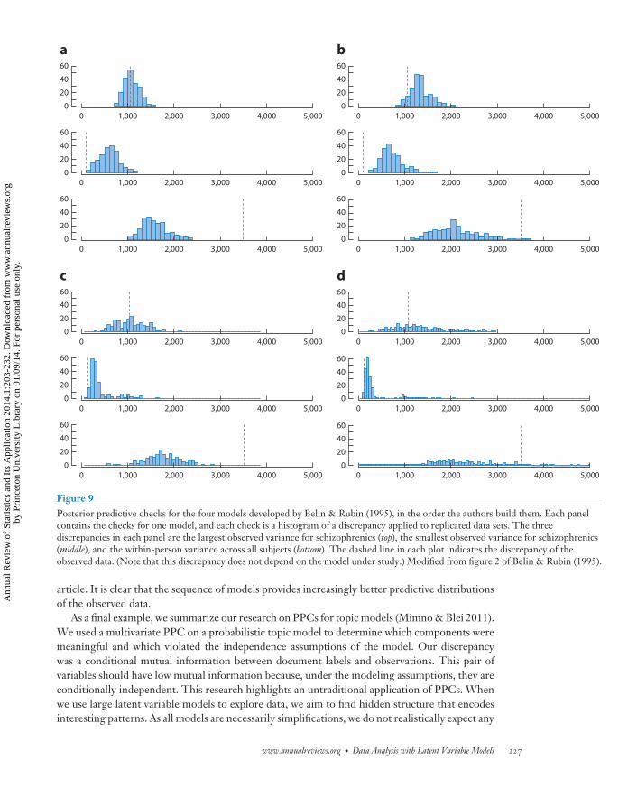
ST01CH10-Blei ARI 4 December 2013 17:0
0 5,0004,0003,0002,0001,000
60
0
20
40
0 5,0004,0003,0002,0001,000
60
0
20
40
0 5,0004,0003,0002,0001,000
60
0
20
40
0 5,0004,0003,0002,0001,000
60
0
20
40
0 5,0004,0003,0002,0001,000
60
0
20
40
0 5,0004,0003,0002,0001,000
60
0
20
40
a b
0 5,0004,0003,0002,0001,000
60
0
20
40
0 5,0004,0003,0002,0001,000
60
0
20
40
0 5,0004,0003,0002,0001,000
60
0
20
40
0 5,0004,0003,0002,0001,000
60
0
20
40
0 5,0004,0003,0002,0001,000
60
0
20
40
0 5,0004,0003,0002,0001,000
60
0
20
40
c d
Figure 9Posterior predictive checks for the four models developed by Belin & Rubin (1995), in the order the authors build them. Each panelcontains the checks for one model, and each check is a histogram of a discrepancy applied to replicated data sets. The threediscrepancies in each panel are the largest observed variance for schizophrenics (top), the smallest observed variance for schizophrenics(middle), and the within-person variance across all subjects (bottom). The dashed line in each plot indicates the discrepancy of theobserved data. (Note that this discrepancy does not depend on the model under study.) Modified from figure 2 of Belin & Rubin (1995).
article. It is clear that the sequence of models provides increasingly better predictive distributionsof the observed data.
As a final example, we summarize our research on PPCs for topic models (Mimno & Blei 2011).We used a multivariate PPC on a probabilistic topic model to determine which components weremeaningful and which violated the independence assumptions of the model. Our discrepancywas a conditional mutual information between document labels and observations. This pair ofvariables should have low mutual information because, under the modeling assumptions, they areconditionally independent. This research highlights an untraditional application of PPCs. Whenwe use large latent variable models to explore data, we aim to find hidden structure that encodesinteresting patterns. As all models are necessarily simplifications, we do not realistically expect any
www.annualreviews.org • Data Analysis with Latent Variable Models 227
Ann
ual R
evie
w o
f St
atis
tics
and
Its
App
licat
ion
2014
.1:2
03-2
32. D
ownl
oade
d fr
om w
ww
.ann
ualr
evie
ws.
org
by P
rinc
eton
Uni
vers
ity L
ibra
ry o
n 01
/09/
14. F
or p
erso
nal u
se o
nly.
ST01CH10-Blei ARI 4 December 2013 17:0
model to be adequate. We can use PPCs to filter out aspects of the model that are not capturingthe data well and to better focus our explorations and visualizations on the meaningful patterns.
6. DISCUSSION
We have reviewed the components of Box’s loop (Figure 1), an iterative process for building andrevising probabilistic models. We posit a model with a graphical model, use generic approximateinference methods to compute with it, and then step out of our assumptions to assess and criticizehow well it fits our observed data. Implementing Box’s loop with modern statistics and machinelearning methods allows us to develop complex probabilistic models to solve real-world data-analysis problems.
Currently, this loop is implemented at the level of a scientific community: Researchers build amodel, derive an inference method, and use the model to solve a problem. Other researchers (orthe same researchers, on a different project) identify how the model falls short, build an improvedmodel, and demonstrate the improvement. One goal for statisticians and computer scientists is todevelop tools—both methodological and technological—for implementing the loop more easilyand more efficiently. These tools will let us develop and use sequences of models before settlingon the appropriate one for the data at hand.
There are several challenges. First, we need approximate inference algorithms that are bothscalable and generic, algorithms that can be used to compute with a large class of models andwith massive data sets. A promising avenue of research in this vein is probabilistic program-ming. Researchers in probabilistic programming are developing software that allows users toeasily specify models and compute approximate posteriors (Gilks & Spiegelhalter 1992, Bishopet al. 2003, McCallum et al. 2009, Stan Development Team 2013; also see http://research.microsoft.com/infernet). These existing systems are a good start, but probabilistic programmingmust be more flexible and more efficient for iterative model building to become a standard practice.
A second challenge is to continue to develop the theory and methods of exploratory data anal-ysis. Exploratory analysis has recently become increasingly important because scientists and otherdata consumers want to discover, understand, and exploit patterns in streams of observationaldata. (Such goals are outside the traditional scientific goal of drawing conclusions from a designedexperiment.) In this spirit, we should continue to develop methods such as PPCs to help navigatelarge data sets with complex models. We should further develop the foundations of data explo-ration, along the lines of Tukey (1962), Good (1983), and Diaconis (1985), to develop principledmethods for exploring observational data.
However, the most important challenges are those we cannot yet identify. The limitationsof our methods will be revealed only when we circle Box’s loop with new data sets and newproblems. In a sense, this is itself an instance of Box’s loop. When we collaborate with scientistsand engineers to solve new data-analysis problems, we can identify how our methods fall short.These shortcomings, in turn, direct us to where and how our methods can be improved.
DISCLOSURE STATEMENT
This material is partly based on research sponsored by DARPA under agreement number FA8750-14-2-0009. The U.S. Government is authorized to reproduce and distribute reprints for Govern-mental purposes notwithstanding any copyright notation thereon. The views and conclusionscontained herein are those of the author and should not be interpreted as necessarily represent-ing the official policies or endorsements, either expressed or implied, of DARPA or the U.S.Government.
228 Blei
Ann
ual R
evie
w o
f St
atis
tics
and
Its
App
licat
ion
2014
.1:2
03-2
32. D
ownl
oade
d fr
om w
ww
.ann
ualr
evie
ws.
org
by P
rinc
eton
Uni
vers
ity L
ibra
ry o
n 01
/09/
14. F
or p
erso
nal u
se o
nly.

ST01CH10-Blei ARI 4 December 2013 17:0
ACKNOWLEDGMENTS
My work is supported by National Science Foundation (NSF) CAREER grant IIS-0745520, NSFBIGDATA grant IIS-1247664, NSF NEURO grant IIS-1009542, Office of Naval Research grantN00014-11-1-0651, and the Alfred P. Sloan foundation. The author is grateful to Martha Benco,Steve Fienberg, Andrew Gelman, Sean Gerrish, Jeremy Manning, Xiao-Li Meng, David Mimno,Donald Rubin, Hal Stern, Chris Wiggins, and Chong Wang for useful comments and discussions.
LITERATURE CITED
Airoldi EM, Blei DM, Fienberg SE, Xing EP. 2008. Mixed membership stochastic blockmodels. J. Mach.Learn. Res. 9:1981–2014
Antoniak CE. 1974. Mixtures of Dirichlet processes with applications to Bayesian nonparametric problems.Ann. Stat. 2:1152–74
Asuncion A, Welling M, Smyth P, Teh YW. 2009. On smoothing and inference for topic models. Proc. Conf.Uncertain. Artif. Intell. 25:27–34
Attias H. 1999. Inferring parameters and structure of latent variable models by variational Bayes. Proc. Conf.Uncertain. Artif. Intell. 15:21–30
Attias H. 2000. A variational Bayesian framework for graphical models. Adv. Neural Inf. Process. Syst. 12:209–15Baker FB. 1992. Item Response Theory. New York: Marcel DekkerBar-Shalom Y, Li XR, Kirubarajan T. 2004. Estimation with Applications to Tracking and Navigation: Theory
Algorithms and Software. New York: WileyBartholomew DJ, Knott M, Moustaki I. 2011. Latent Variable Models and Factor Analysis, Vol. 899: A Unified
Approach. New York: WileyBelin TR, Rubin DB. 1995. The analysis of repeated-measures data on schizophrenic reaction times using
mixture models. Stat. Med. 14:747–68Bell RM, Koren Y. 2007. Lessons from the Netflix prize challenge. ACM SIGKDD Explor. Newsl. 9:75–79Bernardo JM, Smith AFM. 1994. Bayesian Theory. Chichester, UK: WileyBishop CM. 2006. Pattern Recognition and Machine Learning. New York: SpringerBishop CM. 2013. Model-based machine learning. Philos. Trans. R. Soc. A 371:20120222Bishop CM, Spiegelhalter D, Winn J. 2003. VIBES: a variational inference engine for Bayesian networks.
Adv. Neural Inf. Process. Syst. 15:793–800Blei DM. 2012. Probabilistic topic models. Commun. ACM 55:77–84Blei DM, Lafferty JD. 2006. Dynamic topic models. In Proceedings of the 23rd International Conference on
Machine Learning, ed. W Cohen, A Moore, pp. 113–20. New York: Assoc. Comput. Mach.Blei DM, Lafferty JD. 2007. A correlated topic model of science. Ann. Appl. Stat. 1:17–35Blei DM, Ng AY, Jordan MI. 2003. Latent Dirichlet allocation. J. Mach. Learn. Res. 3:993–1022Box GEP. 1976. Science and statistics. J. Am. Stat. Assoc. 71:791–99Box GEP. 1980. Sampling and Bayes’ inference in scientific modelling and robustness. J. R. Stat. Soc. A
143:383–430Box GEP, Draper NR. 1987. Empirical Model-Building and Response Surfaces. New York: WileyBox GEP, Hill WJ. 1967. Discrimination among mechanistic models. Technometrics 9:57–71Box GEP, Hunter WG. 1962. A useful method for model-building. Technometrics 4:301–18Box GEP, Hunter WG. 1965. The experimental study of physical mechanisms. Technometrics 7:23–42Box GEP, Tiao GC. 1973. Bayesian Inference in Statistical Analysis. New York: WileyBrown LD. 1986. Fundamentals of Statistical Exponential Families with Applications in Statistical Decision Theory.
Hayward, CA: Inst. Math. Stat.Claeskens G, Hjort NL. 2008. Model Selection and Model Averaging. New York: Cambridge Univ. PressClinton J, Jackman S, Rivers D. 2004. The statistical analysis of roll call data. Am. Polit. Sci. Rev. 98:355–70Collins M, Dasgupta S, Schapire R. 2002. A generalization of principal component analysis to the exponential
family. Adv. Neural Inf. Process. Syst. 14:617–24Cook RD, Weisberg S. 1982. Residuals and Influence in Regression. London: Chapman & Hall
www.annualreviews.org • Data Analysis with Latent Variable Models 229
Ann
ual R
evie
w o
f St
atis
tics
and
Its
App
licat
ion
2014
.1:2
03-2
32. D
ownl
oade
d fr
om w
ww
.ann
ualr
evie
ws.
org
by P
rinc
eton
Uni
vers
ity L
ibra
ry o
n 01
/09/
14. F
or p
erso
nal u
se o
nly.
ST01CH10-Blei ARI 4 December 2013 17:0
Dawid AP, Lauritzen SL. 1993. Hyper Markov laws in the statistical analysis of decomposable graphicalmodels. Ann. Stat. 21:1272–317
Dempster AP, Laird NM, Rubin DB. 1977. Maximum likelihood from incomplete data via the EM algorithm.J . R. Stat. Soc. B. 36:1–38
Diaconis P. 1985. Theories of data analysis: from magical thinking through classical statistics. In ExploringData: Tables, Trends, and Shapes, ed. DC Hoaglin, F Mosteller, JW Tukey, pp. 1–36. New York: Wiley
Durbin R, Eddy SR, Krogh A, Mitchison G. 1998. Biological Sequence Analysis: Probabilistic Models of Proteinsand Nucleic Acids. New York: Cambridge Univ. Press
Efron B. 2013. Empirical Bayes modeling, computation, and accuracy. Tech. rep. 263, Div. Biostat., Stanford Univ.,Stanford, CA. http://statweb.stanford.edu/∼ckirby/brad/papers/2013EBModeling.pdf
Efron B, Morris C. 1973. Combining possibly related estimation problems. J. R. Stat. Soc. B 35:379–421Erosheva E, Fienberg S, Lafferty J. 2004. Mixed-membership models of scientific publications. Proc. Natl.
Acad. Sci. USA 101(Suppl. 1):5220–27Erosheva EA, Fienberg SE, Joutard C. 2007. Describing disability through individual-level mixture models
for multivariate binary data. Ann. Appl. Stat. 1:502–37Ferguson TS. 1973. A Bayesian analysis of some nonparametric problems. Ann. Stat. 1:209–30Geisser S. 1975. The predictive sample reuse method with applications. J. Am. Stat. Assoc. 70:320–28Gelfand AE, Smith AFM. 1990. Sampling-based approaches to calculating marginal densities. J. Am. Stat.
Assoc. 85:398–409Gelman A, Carlin JB, Stern HS, Rubin DB. 1995. Bayesian Data Analysis. London: Chapman & HallGelman A, Hill J. 2007. Data Analysis Using Regression and Multilevel/Hierarchical Models. New York: Cambridge
Univ. PressGelman A, Meng X-L, Stern H. 1996. Posterior predictive assessment of model fitness via realized discrep-
ancies. Stat. Sin. 6:733–807Gelman A, Shalizi CR. 2012. Philosophy and the practice of Bayesian statistics. Br. J. Math. Stat. Psychol.
66:8–38Gelman A, Van Mechelen I, Verbeke G, Heitjan DF, Meulders M. 2005. Multiple imputation for model
checking: completed-data plots with missing and latent data. Biometrics 61:74–85Geman S, Geman D. 1984. Stochastic relaxation, Gibbs distributions and the Bayesian restoration of images.
IEEE Trans. Pattern Anal. Mach. Intell. 6:721–41Gershman SJ, Blei DM. 2012. A tutorial on Bayesian nonparametric models. J. Math. Psychol. 56:1–12Ghahramani Z. 2012. Bayesian nonparametrics and the probabilistic approach to modelling. Philos. Trans. R.
Soc. A 371:1984Ghahramani Z, Beal MJ. 2001. Propagation algorithms for variational Bayesian learning. Adv. Neural Inf.
Process. Syst. 13:507–13Gilks WR, Thomas A, Spiegelhalter DJ. 1992. A language and program for complex Bayesian modelling.
Statistician 43:169–77Good IJ. 1983. The philosophy of exploratory data analysis. Philos. Sci. 50:283–95Good IJ. 2009 (1983). Subjective probability as the measure of a non-measurable set. In Good Thinking: The
Foundations of Probability and Its Applications, pp. 73–82. Mineola, NY: DoverGuttman I. 1967. The use of the concept of a future observation in goodness-of-fit problems. J. R. Stat. Soc.
B 29:83–100Hastings WK. 1970. Monte Carlo sampling methods using Markov chains and their applications. Biometrika
57:97–109Hjort NL, Holmes C, Muller P, Walker SG, eds. 2010. Bayesian Nonparametrics. New York: Cambridge Univ.
PressHoffman MD, Blei DM, Wang C, Paisley J. 2013. Stochastic variational inference. J. Mach. Learn. Res.
14:1303–47Hotelling H. 1933. Analysis of a complex of statistical variables into principal components. J. Educ. Psychol.
24:417–41Hotelling H. 1936. Relations between two sets of variates. Biometrika 28:321–77Ishwaran H, Rao JS. 2005. Spike and slab variable selection: frequentist and Bayesian strategies. Ann. Stat.
33:730–73
230 Blei
Ann
ual R
evie
w o
f St
atis
tics
and
Its
App
licat
ion
2014
.1:2
03-2
32. D
ownl
oade
d fr
om w
ww
.ann
ualr
evie
ws.
org
by P
rinc
eton
Uni
vers
ity L
ibra
ry o
n 01
/09/
14. F
or p
erso
nal u
se o
nly.
ST01CH10-Blei ARI 4 December 2013 17:0
Jordan MI, ed. 1999. Learning in Graphical Models. Cambridge, MA: MIT PressJordan MI. 2004. Graphical models. Stat. Sci. 19:140–55Jordan MI, Ghahramani Z, Jaakkola TS, Saul LK. 1999. An introduction to variational methods for graphical
models. Mach. Learn. 37:183–233Kalman RE. 1960. A new approach to linear filtering and prediction problems. Trans. ASME J. Basic Eng.
82:35–45Kass RE, Raftery AE. 1995. Bayes factors. J. Am. Stat. Assoc. 90:773–95Knowles DA, Minka TP. 2011. Non-conjugate variational message passing for multinomial and binary re-
gression. Adv. Neural Inf. Process. Syst. 24:1701–9Koller D, Friedman N. 2009. Probabilistic Graphical Models: Principles and Techniques. Cambridge, MA: MIT
PressKoren Y, Bell R, Volinsky C. 2009. Matrix factorization techniques for recommender systems. Computer
42:30–37Krnjajic M, Kottas A, Draper D. 2008. Parametric and nonparametric Bayesian model specification: a case
study involving models for count data. Comput. Stat. Data Anal. 52:2110–28Kullback S, Leibler RA. 1951. On information and sufficiency. Ann. Math. Stat. 22:79–86Lauritzen SL. 2007. Discussion of some aspects of model selection for prediction: article of Chakrabarti and
Ghosh. In Bayesian Statistics 8, ed. JM Bernardo, MJ Bayarri, JO Berger, AP David, D Heckerman, et al.,pp. 84–90. Oxford, UK: Oxford Univ. Press
Lee DD, Seung HS. 1999. Learning the parts of objects by non-negative matrix factorization. Nature 401:788–91
Lehmann EL. 1990. Model specification: the views of Fisher and Neyman, and later developments. Stat. Sci.5(2):160–68
MacKay DJC. 2003. Information Theory, Inference, and Learning Algorithms. New York: Cambridge Univ. PressMcAuliffe JD, Pachter L, Jordan MI. 2004. Multiple-sequence functional annotation and the generalized
hidden Markov phylogeny. Bioinformatics 20:1850–60McCallum A, Schultz K, Singh S. 2009. FACTORIE: probabilistic programming via imperatively defined
factor graphs. Adv. Neural Inf. Process. Syst. 22:1249–57McCullagh P, Nelder JA. 1989. Generalized Linear Models. London: Chapman & HallMeng X-L. 1994. Posterior predictive p-values. Ann. Stat. 22:1142–60Metropolis N, Rosenbluth AW, Rosenbluth MN, Teller AH, Teller E. 1953. Equations of state calculations
by fast computing machines. J. Chem. Phys. 21:1087–92Mimno D, Blei DM. 2011. Bayesian checking for topic models. In Proceedings of the Conference on Empirical
Methods in Natural Language Processing, ed. P Merlo, pp. 227–37. Stroudsburg, PA: Assoc. Comput.Linguist.
Mohamed S, Ghahramani Z, Heller K. 2008. Bayesian exponential family PCA. Adv. Neural Inf. Process. Syst.21:1089–96
Morris CN. 1983. Parametric empirical Bayes inference: theory and applications. J. Am. Stat. Assoc. 78:47–65Murphy KP. 2013. Machine Learning: A Probabilistic Approach. Cambridge, MA: MIT PressNeal RM, Hinton GE. 1999. A view of the EM algorithm that justifies incremental, sparse, and other variants.
In Learning in Graphical Models, ed. MI Jordan, pp. 355–68. Cambridge, MA: MIT PressNelder JA, Wedderburn RWM. 1972. Generalized linear models. J. R. Stat. Soc. A 135:370–84Pearl J. 1988. Probabilistic Reasoning in Intelligent Systems: Networks of Plausible Inference. New York: Morgan
Kaufmann Publ.Pearson K. 1901. On lines and planes of closest fit to systems of points. Lond. Edinb. Dublin Philos. Mag. J. Sci.
6:559–72Peterson C, Anderson JR. 1987. A mean field theory learning algorithm for neural networks. Complex Syst.
1:995–1019Popper KR. 1959. The Logic of Scientific Discovery. London: HutchinsonPritchard JK, Stephens M, Donnelly P. 2000. Inference of population structure using multilocus genotype
data. Genetics 155:945–59Rabiner LR. 1989. A tutorial on hidden Markov models and selected applications in speech recognition. Proc.
IEEE 77:257–86
www.annualreviews.org • Data Analysis with Latent Variable Models 231
Ann
ual R
evie
w o
f St
atis
tics
and
Its
App
licat
ion
2014
.1:2
03-2
32. D
ownl
oade
d fr
om w
ww
.ann
ualr
evie
ws.
org
by P
rinc
eton
Uni
vers
ity L
ibra
ry o
n 01
/09/
14. F
or p
erso
nal u
se o
nly.
ST01CH10-Blei ARI 4 December 2013 17:0
Robbins H. 1980. An empirical Bayes estimation problem. Proc. Natl. Acad. Sci. USA 77:6988–89Robbins H, Monro S. 1951. A stochastic approximation method. Ann. Math. Stat. 22:400–7Robert CP, Casella G. 2004. Monte Carlo Statistical Methods. New York: SpringerRoweis S. 1998. EM algorithms for PCA and SPCA. Adv. Neural Inf. Process. Syst. 10:626–32Rubin DB. 1984. Bayesianly justifiable and relevant frequency calculations for the applied statistician. Ann.
Stat. 12:1151–72Rue H, Martino S, Chopin N. 2009. Approximate Bayesian inference for latent Gaussian models by using
integrated nested Laplace approximations. J. R. Stat. Soc. B 71:319–92Salakhutdinov R, Mnih A. 2008. Probabilistic matrix factorization. Adv. Neural Inf. Process. Syst. 20:1257–64Saul LK, Jordan MI. 1996. Exploiting tractable substructures in intractable networks. Adv. Neural Inf. Process.
Syst. 8:486–92Siepel A, Haussler D. 2004. Combining phylogenetic and hidden Markov models in biosequence analysis.
J. Comput. Biol. 11:413–28Skrondal A, Rabe-Hesketh S. 2007. Latent variable modelling: a survey. Scand. J. Stat. 34:712–45Smola AJ, Vishwanathan SVN, Eskin E. 2003. Laplace propagation. Adv. Neural Inf. Process. Syst. 16:441–48Stan Development Team. 2013. Stan: A C++ Library for Probability and Sampling, Version 1.3. http://
mc-stan.orgSteyvers M, Griffiths T. 2006. Probabilistic topic models. In Latent Semantic Analysis: A Road to Meaning, ed.
T Landauer, D McNamara, S Dennis, W Kintsch, pp. 424–40. London: Laurence ErlbaumStone M. 1974. Cross-validatory choice and assessment of statistical predictions. J. R. Stat. Soc. B 36:111–47Teh YW, Jordan MI. 2008. Hierarchical Bayesian nonparametric models with applications. In Bayesian Non-
parametrics, ed. NL Hjort, C Holmes, P Muller, SG Walker, pp. 158–207. New York: Cambridge Univ.Press
Thomson G. 1939. The factorial analysis of human ability. Br. J. Educ. Psychol. 9:188–95Thurstone LL. 1931. Multiple factor analysis. Psychol. Rev. 38:406–27Thurstone LL. 1938. Primary Mental Abilities. Chicago: Univ. Chicago PressTierney L, Kass RE, Kadane JB. 1989. Fully exponential Laplace approximations to expectations and variances
of nonpositive functions. J. Am. Stat. Assoc. 84:710–16Tipping ME, Bishop CM. 1999. Probabilistic principal component analysis. J. R. Stat. Soc. B 61:611–22Tukey JW. 1962. The future of data analysis. Ann. Math. Stat. 33:1–67van Dyk DA, Kang H. 2004. Highly structured models for spectral analysis in high-energy astrophysics. Stat.
Sci. 19:275–93Wainwright MJ, Jordan MI. 2008. Graphical models, exponential families, and variational inference. Found.
Trends Mach. Learn. 1:1–305Wang C, Blei DM. 2013. Variational inference in nonconjugate models. J. Mach. Learn. Res. 14:1005–1031West M, Harrison J. 1997. Bayesian Forecasting and Dynamic Models. Berlin: SpringerWiegerinck W. 2000. Variational approximations between mean field theory and the junction tree algorithm.
Proc. Conf. Uncertain. Artif. Intell. 16:626–33Xing EP, Jordan MI, Russell S. 2003. A generalized mean field algorithm for variational inference in expo-
nential families. Proc. Conf. Uncertain. Artif. Intell. 19:583–91
232 Blei
Ann
ual R
evie
w o
f St
atis
tics
and
Its
App
licat
ion
2014
.1:2
03-2
32. D
ownl
oade
d fr
om w
ww
.ann
ualr
evie
ws.
org
by P
rinc
eton
Uni
vers
ity L
ibra
ry o
n 01
/09/
14. F
or p
erso
nal u
se o
nly.
ST01-FrontMatter ARI 25 November 2013 21:12
Annual Review ofStatistics and ItsApplication
Volume 1, 2014ContentsWhat Is Statistics?
Stephen E. Fienberg � � � � � � � � � � � � � � � � � � � � � � � � � � � � � � � � � � � � � � � � � � � � � � � � � � � � � � � � � � � � � � � � � � � � � � � � � � � 1
A Systematic Statistical Approach to Evaluating Evidence fromObservational StudiesDavid Madigan, Paul E. Stang, Jesse A. Berlin, Martijn Schuemie,
J. Marc Overhage, Marc A. Suchard, Bill Dumouchel, Abraham G. Hartzema,and Patrick B. Ryan � � � � � � � � � � � � � � � � � � � � � � � � � � � � � � � � � � � � � � � � � � � � � � � � � � � � � � � � � � � � � � � � � � � � � � � �11
The Role of Statistics in the Discovery of a Higgs BosonDavid A. van Dyk � � � � � � � � � � � � � � � � � � � � � � � � � � � � � � � � � � � � � � � � � � � � � � � � � � � � � � � � � � � � � � � � � � � � � � � � � � � �41
Brain Imaging AnalysisF. DuBois Bowman � � � � � � � � � � � � � � � � � � � � � � � � � � � � � � � � � � � � � � � � � � � � � � � � � � � � � � � � � � � � � � � � � � � � � � � � � � �61
Statistics and ClimatePeter Guttorp � � � � � � � � � � � � � � � � � � � � � � � � � � � � � � � � � � � � � � � � � � � � � � � � � � � � � � � � � � � � � � � � � � � � � � � � � � � � � � � � �87
Climate Simulators and Climate ProjectionsJonathan Rougier and Michael Goldstein � � � � � � � � � � � � � � � � � � � � � � � � � � � � � � � � � � � � � � � � � � � � � � � � � 103
Probabilistic ForecastingTilmann Gneiting and Matthias Katzfuss � � � � � � � � � � � � � � � � � � � � � � � � � � � � � � � � � � � � � � � � � � � � � � � � 125
Bayesian Computational ToolsChristian P. Robert � � � � � � � � � � � � � � � � � � � � � � � � � � � � � � � � � � � � � � � � � � � � � � � � � � � � � � � � � � � � � � � � � � � � � � � � � 153
Bayesian Computation Via Markov Chain Monte CarloRadu V. Craiu and Jeffrey S. Rosenthal � � � � � � � � � � � � � � � � � � � � � � � � � � � � � � � � � � � � � � � � � � � � � � � � � � � 179
Build, Compute, Critique, Repeat: Data Analysis with LatentVariable ModelsDavid M. Blei � � � � � � � � � � � � � � � � � � � � � � � � � � � � � � � � � � � � � � � � � � � � � � � � � � � � � � � � � � � � � � � � � � � � � � � � � � � � � � � 203
Structured Regularizers for High-Dimensional Problems: Statistical andComputational IssuesMartin J. Wainwright � � � � � � � � � � � � � � � � � � � � � � � � � � � � � � � � � � � � � � � � � � � � � � � � � � � � � � � � � � � � � � � � � � � � � 233
High-Dimensional Statistics with a View Toward Applications in BiologyPeter Buhlmann, Markus Kalisch, and Lukas Meier � � � � � � � � � � � � � � � � � � � � � � � � � � � � � � � � � � � � � 255
v
Ann
ual R
evie
w o
f St
atis
tics
and
Its
App
licat
ion
2014
.1:2
03-2
32. D
ownl
oade
d fr
om w
ww
.ann
ualr
evie
ws.
org
by P
rinc
eton
Uni
vers
ity L
ibra
ry o
n 01
/09/
14. F
or p
erso
nal u
se o
nly.

ST01-FrontMatter ARI 25 November 2013 21:12
Next-Generation Statistical Genetics: Modeling, Penalization, andOptimization in High-Dimensional DataKenneth Lange, Jeanette C. Papp, Janet S. Sinsheimer, and Eric M. Sobel � � � � � � � � � � � � � 279
Breaking Bad: Two Decades of Life-Course Data Analysis inCriminology, Developmental Psychology, and BeyondElena A. Erosheva, Ross L. Matsueda, and Donatello Telesca � � � � � � � � � � � � � � � � � � � � � � � � � � � � 301
Event History AnalysisNiels Keiding � � � � � � � � � � � � � � � � � � � � � � � � � � � � � � � � � � � � � � � � � � � � � � � � � � � � � � � � � � � � � � � � � � � � � � � � � � � � � � � � 333
Statistical Evaluation of Forensic DNA Profile EvidenceChristopher D. Steele and David J. Balding � � � � � � � � � � � � � � � � � � � � � � � � � � � � � � � � � � � � � � � � � � � � � � 361
Using League Table Rankings in Public Policy Formation:Statistical IssuesHarvey Goldstein � � � � � � � � � � � � � � � � � � � � � � � � � � � � � � � � � � � � � � � � � � � � � � � � � � � � � � � � � � � � � � � � � � � � � � � � � � � 385
Statistical EcologyRuth King � � � � � � � � � � � � � � � � � � � � � � � � � � � � � � � � � � � � � � � � � � � � � � � � � � � � � � � � � � � � � � � � � � � � � � � � � � � � � � � � � � � 401
Estimating the Number of Species in Microbial Diversity StudiesJohn Bunge, Amy Willis, and Fiona Walsh � � � � � � � � � � � � � � � � � � � � � � � � � � � � � � � � � � � � � � � � � � � � � � � 427
Dynamic Treatment RegimesBibhas Chakraborty and Susan A. Murphy � � � � � � � � � � � � � � � � � � � � � � � � � � � � � � � � � � � � � � � � � � � � � � � 447
Statistics and Related Topics in Single-Molecule BiophysicsHong Qian and S.C. Kou � � � � � � � � � � � � � � � � � � � � � � � � � � � � � � � � � � � � � � � � � � � � � � � � � � � � � � � � � � � � � � � � � � 465
Statistics and Quantitative Risk Management for Banking and InsurancePaul Embrechts and Marius Hofert � � � � � � � � � � � � � � � � � � � � � � � � � � � � � � � � � � � � � � � � � � � � � � � � � � � � � � � 493
vi Contents
Ann
ual R
evie
w o
f St
atis
tics
and
Its
App
licat
ion
2014
.1:2
03-2
32. D
ownl
oade
d fr
om w
ww
.ann
ualr
evie
ws.
org
by P
rinc
eton
Uni
vers
ity L
ibra
ry o
n 01
/09/
14. F
or p
erso
nal u
se o
nly.