BSR: A Statistic-based Approach for Establishing and Refining Software Process Performance Baseline

Qing Wang1, Nan Jiang1,2, Lang Gou1,2, Xia Liu1,2, Mingshu Li1, Yongji Wang1 1Institute of Software, Chinese Academy of Sciences

4# South Fourth Street, Zhong Guan Cun Beijing 100080, P.R. CHINA

Tel: +86(10)62544128 2Graduate University of Chinese Academy of Sciences,

19# Yuquan Road, Shijingshan District Beijing 100039, P.R. CHINA

{wq, jiangnan, goulang, liuxia, mingshu, ywang}@itechs.iscas.ac.cn

ABSTRACT High-level process management is quantitative management. The Process Performance Baseline (PPB) of process or subprocess under statistical management is the most important concept. It is the basis of process control and improvement. The existing methods for establishing process baseline are too coarse-grained or have some limitation, which lead to inaccurate or ineffective quantitative management. In this paper, we propose an approach called BSR (Baseline-Statistic-Refinement) for establishing and refining software process performance baseline, and present the experience result to validate its effectiveness for quantitative process management.

Categories and Subject Descriptors D.2.8 [Software Engineering]: Metrics – Process metrics

General Terms Experimentation, Management, Measurement.

Keywords Measurement, Quantitative process management, Process performance baseline, Software process improvement

1. INTRODUCTION Software process techniques are widely applied in the development of software-intensive systems. Under software process, how to estimate the schedule, effort, size, and defect density as well as how to control the actual performance against estimation are crucial. Is the process capable of delivering products that meet requirements? Does the performance of the process meet the business needs of the organization?[7] The measurement and quantitative management for software process are necessary to solve these problems.

Quantitative management for software process is used to indicate whether the process has achieved its predictable goal and what causes exist when significant deviation appears. In fact, many software quality management models such as CMM/CMMI[3][4], ISO9000:2000[14] and ISO/IEC15504[13], all stress the importance of the measurement and quantitative management for software process. In CMMI, Quantitative Process Management is a characteristic of capability level 4. ISO9000: 2000 emphasizes that “The organizations shall apply suitable methods for monitoring, where applicable, measurement of the quality management system processes”. Other quality models and standards, such as ISO/IEC15504, also require measurement. So, measurement and quantitative management for software process have become the general requirements of quality management system.

There are several methods (e.g. PSM-Practical Software Measurement, GDM-Goal Driven Measurement) and techniques (e.g. Six Sigma[20], SPC[5][6][15], Ishikawa’s seven basic tools[12]) for software process measurement and quantitative control. Performance and capability are two key factors to measure whether software process is mature or not. PPB is the characterization of the actual results achieved by following a process, which is used as a benchmark for comparing actual process performance and capability against expected process performance and capability. As we know, software process is different from traditional process. Its performance doesn’t depend on the device of product line, but depends on the people who execute the process. Different people or teams have different performance and capability even use the same device. The baseline of software process is difficult to establish precisely; it should be evolved and refined based on the historical data with the process improvement. Many researches try to address it. Unfortunately, most of them depend on the benchmark or the experience in the industry. It can be used to provide some help in estimation but lacks accuracy for quantitative management.

In this paper, we propose an approach called BSR (Baseline-Statistic-Refinement) to establish and refine software process performance baseline. Focusing on objective process that has definite capability, the BSR approach provides methods and steps to establish and refine the performance baseline based on statistics techniques. We have applied the approach in a number of organizations to validate that the approach can establish an effective baseline for process control and improvement. Also,

Permission to make digital or hard copies of all or part of this work for personal or classroom use is granted without fee provided that copies are not made or distributed for profit or commercial advantage and that copies bear this notice and the full citation on the first page. To copy otherwise, or republish, to post on servers or to redistribute to lists, requires prior specific permission and/or a fee. ICSE'06, May 20-28, 2006, Shanghai, China. Copyright 2006 ACM 1-59593-085-X/06/0005...$5.00.

585

BSR is very helpful for software organizations to apply quantitative management at CMMI Level 4.

2. RELATED WORK Benchmark is a technique to establish the process performance baseline using external comparisons. The ISBSG[11] organization collects data from different projects and organizations. A new project or a group of completed projects can be benchmarked against similar projects in the ISBSG Repository. In this technique, projects are compared against the median value and quartiles values from a selected group of projects in the ISBSG Repository. These values are a group of attributes that are known to influence development productivity, namely development platform, language type and maximum team size. The Benchmark in ISBSG is helpful for comparing the performance among projects, and it is also helpful for estimation when the project lacks historical data. However, for quantitative process control, it is coarse-grained. Basically, ISBSG focuses on the productivity of software products. Effort distribution among the basic process activities, such as project management, requirement analysis, design, implementation and test, are also provided[11]. However, quantitative management is focused on the identified processes or subprocesses which are significant for process improvement. These processes or subprocesses have small granularity against general engineering phase. It may not be the best but it is stable. It can be managed quantitatively too. So using the benchmark to establish the performance baseline will lack effective pertinence for managing these processes quantitatively.

The Experience Factory (EF)[1][2] aims to establish an organizational infrastructure to facilitate systematic and continuous organizational learning through the sharing and reuse of experience in software engineering. EF teaches the organization to observe itself, collect data about itself, build models and draw conclusions based on the data, package the experience for further reuse, and most importantly to feed the experience back to the organization and for sharing it within and outside the organization. A number of organizations have adopted some of the principles of experience factories into their own businesses, such as the Software Engineering Laboratory at NASA[1][18] and Daimler Benz[8]. In practice, the EF method is implemented by first putting the organization in place, which is to establish the baseline. EF does not focus itself on process performance baseline. But the experience fed back in EF method is very useful in establishing the process baseline. BSR approach adopts the principle in its method.

SPC (Statistical Process Control)[5][6][19][15] is the method widely used to manage process quantitatively. According to [16][17], SPC has been applied in many high-level maturity organizations. The goal of statistical process control is to monitor and control the process’s stability. SPC needs three control limits, which are based on the population statistical parameters called average μ and standard deviation σ. Generally, the two statistics come from historical data or current large sample. Actually, we often take μ and σ as the performance and capability of process respectively. In many methods, the two population statistics parameters are calculated from large sample data. It means the large data sample is needed before SPC was applied appropriately. In addition, SPC is often used to monitor stable process and make an alert when an exception occurs.

How to measure these data before the process is stable, how to provide information for process improvement and how to evolve the performance baseline are the barriers of process improvement. Institute of Software, Chinese Academy of Sciences (ISCAS) research and present a method called BSR to address establishing and refining performance baseline based on statistics through the lifecycle of process improvement.

3. BSR APPROACH As we know, either measurement or management needs cost. So we should apply these appropriately. For quantitative management, the first thing is to identify which processes should be placed under quantitative control, and then collect data, construct the sample to be measured to indicate the status of the process. In general, only those processes with affirmatory goal(s), resource(s) and skill(s) may be evolved to the stable status, which is also declaimed in PSP[9] and TSP[10]. ISCAS presents a software process modeling method[24] to help software organizations establish and model their processes with determined capabilities. In this modeling method, we organize the process with definite goal, knowledge and performance as a basic process unit, such as, a java programming processes which people has lower, middle or higher productivity. We call these process units as process agents. These process agents have relationship with each other and are described in the method too. They are the entities of process quantitatively control. BSR collects and measures the data of these processes, establishes their performance baseline, and refines them continuously.

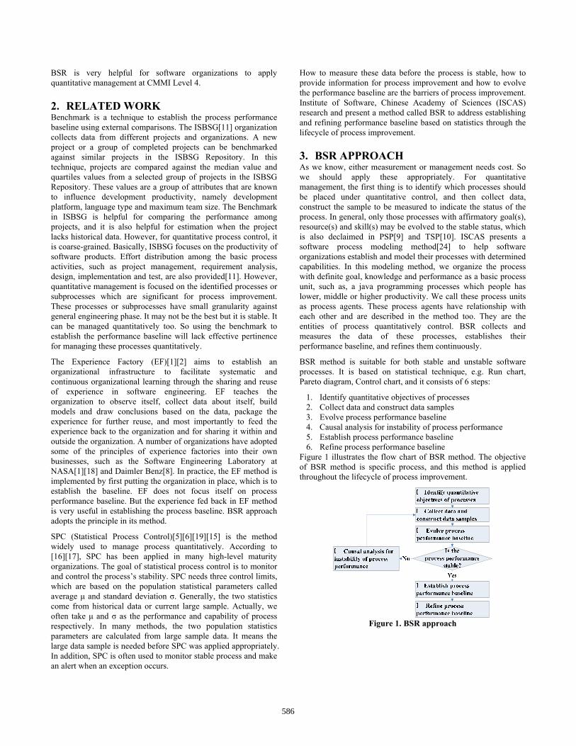
BSR method is suitable for both stable and unstable software processes. It is based on statistical technique, e.g. Run chart, Pareto diagram, Control chart, and it consists of 6 steps:

1. Identify quantitative objectives of processes 2. Collect data and construct data samples 3. Evolve process performance baseline 4. Causal analysis for instability of process performance 5. Establish process performance baseline 6. Refine process performance baseline

Figure 1 illustrates the flow chart of BSR method. The objective of BSR method is specific process, and this method is applied throughout the lifecycle of process improvement.

Figure 1. BSR approach

586

3.1 Identifying Quantitative Objectives of Processes The first step in establishing and refining process performance baseline is to identify the processes and their quantitative objectives, which allows us to concentrate on the necessary and higher priority process improvement. At the same time, it also makes the quantitative management economical and objectively realizable.

The following principles should be referred when identifying the objective processes:

Goal-Driven Principle: Selection of objective processes is based upon the business goals of the organization.

Determinateness Principle: the determinateness of process is affected by human, environment, technique and resource. We should model, construct or select the process with specific resource, skill, and domain knowledge. Their performance and capability can be compared and improved.

Stability Principle: the process we select could be stable. In other words, we can get a stable process by process improvement.

3.2 Collecting Data and Constructing Data Samples With the processes and its quantitative objectives identified, the next step is to collect data and construct data samples. First, it is necessary to determine which measures are useful for describing process performance. The Goal-Question-Metric paradigm or the Practical Software Measurement is an effective method that can be used to determine measures that provide insight into the process performance.

When the proper measures are determined, we should collect data to affect the quantitative objectives of process. The historical data of related projects are also needed to construct the data sample. The data must be comparable to ensure a reasonable baseline is established. For example, if we compare the defect density (defect number in unit size) of modules that have different complexity, the variations of data will be large, and the cause of large variations can not be eliminated. Thus, we will not get a reasonable process performance baseline. In this case, we should assess each module for complexity and difficulty by a weighting factor.

3.3 Evolving Process Performance Baseline Process Performance Baseline contains two important indicators of process: performance and capability. As Figure 2 illustrates, the process performance is “a measure of actual results achieved by following a process” [19], and the process capability is “the range of expected results that can be achieved by following a process.” [19].

Figure 2. Process performance and capability

Under process management, we will collect data according to plan and specified procedure. Measuring these data by appropriate

algorithm should provide helpful information to guide the process improvement. How to measure the data on hand and analyze why the quality is not good are challenges. In this period, there is not a large data sample, and an adequate performance baseline has not been established. We do not know what reasonable value we can expect. BSR uses run chart to analyze the distribution of data sample and find the information for improvement. It can evolve the performance baseline with the continuous improvement.

In run chart, we consider two statistics: average μ and standard deviation σ. For a sample X={x1, x2,…, xn}, we can calculate the average and the standard deviation by the formulas as shown:

nxn

ii∑

=

=1

μ , )1()(1

2 −−= ∑=

nxn

ii μσ

Where μ is the central line in the run chart, and μ±σ is the run limits. Figure 3 shows an example of a run chart.

Figure 3. Run chart

Basically, process has a desired value of performance, such as the variance between plan schedule and actual schedule is zero. The two statistics reflect the population information of process. The larger the difference between μ and the desired value, the worse performance is. The larger the standard deviation σ, the more unstable the process’s capability is.

Table 1 lists the basic principle of analysis.

Table 1. Analysis for run chart

μ σ Problem of the process Action of improvement

Good Large

Process performance is good, but the process is unstable.

Analysis the cause of the instability, such as difference of team member’s capability, morale of engineers, and lack of management and monitoring.

Bad Small

Process performance is bad, but the process is stable.

Analysis the cause of the bad performance, such as inaccurate estimation, lack of engineer’s experience, and inefficient method.

Bad Large

Process performance is bad, and the process is unstable.

Analysis the cause of the bad performance and instability. The causes include all causes mentioned above.

Good Small

Process performance is good, and the process is stable.

No action, we can go to Step 5 to establish the baseline.

Normally, average and standard deviation provide general information and direction for process improvement. The data points that exceed the limit should be analyzed further.

3.4 Causal Analysis for Instability of Process Performance The statistics μ and σ of measured data sample reflect the population information of process. Based on the data, the exceptional point should be analyzed to find and remove the

587

specific cause that raise the exception. Statistical methods such as Pareto, Causal-and-effect diagram, and Scatter chart are helpful.

A Pareto diagram is a frequency chart of bars in descending order; the frequency bars are usually associated with types or causes of problems. By arranging the causes based on problem frequency, a Pareto diagram can identify the few causes that account for the majority of problems. It indicates which problems should be solved first in process improvement. Pareto analysis is commonly referred to the 80-20 principle (20% of the causes account for 80% of the problems). It helps in identifying areas that cause most of the problems, which normally means we get the best return on investment when we fix them. More discussion about Pareto diagram is in the reference [15].

There are some other tools for causal analysis, such as Causal-and-effect diagram and Scatter chart [15]. We can use these tools to identify the cause of process variations, and find a proper approach to improve process performance and capability. When we implement process improvement, we can perform step 2 to step 4 repeatedly, until the process is stable enough to establish process performance baseline.

3.5 Establishing Process Performance Baseline Along with the improvement of process, we find the average is getting close to the desired value, and the standard deviation is getting narrower. They will be evolved in an accepted and stable scope. Most of the data points fall in the run limits (μ±σ). The baseline has been established. The process is regarded as being in a stable state. Subsequently, we can regard μ and σ as the population statistics and will be used in Shewhart 3σ control chart. [4].

3.6 Refining Process Performance Baseline In last step, we evolved the baseline of process performance and got the population statistics of process objective. We can upgrade into Quantitative Management Level. SPC was often applied to here. Shewhart 3σ control charts were the first option. Based on SPC, we can:

Determine whether processes are behaving consistently or have stable trends

Identify processes where the performance is within natural bounds that are consistent across process implementation teams

Identify processes that show unusual (e.g., sporadic or unpredictable) behavior

Identify and analyze the causes of defects and other problems that can be improved

Here, at first, the quality and process performance were understood in statistical terms and were managed throughout the life of the processes. The causes of process variation are identified, the appropriate corrective actions are taken, and the process is improved continuously. Subsequently, the process is improved based on a quantitative understanding of common causes of variation inherent in process. Process performance is refined continuously.

The approach to refine process performance baseline is analyzing the variations that are found in the Shewhart 3σ control chart. If

the performance values fall outside the control limits or indicate a trend, the process has a variation.

Software process is different from manufacturing process. This means the principle of determining whether the process is out of control and how to analyze the problem should be changed and improved. For example, if the defect density data always fall in the area between central line and lower control limit in Shewhart 3σ control chart, it is a problem in manufacturing process. But in software process, it may be a good phenomenon, since it indicates quality has been improved. In this instance, we do not need to take corrective actions, just refine the performance baseline.

4. EXPERIENCE RESULT OF BSR The BSR approach has been applied in more than 50 software organizations. We select three organizations that want to achieve high software capability maturity level to practice the BSR approach. BSR was applied throughout their process improvement lifecycle from lower level to higher level. The overview of the three organizations is shown in Table 2.

Table 2. Organizations overview

Org. Scale (People) Domain Current

CMM Level A 120 Software process improvement,

software quality assurance CMMI 4

B 500 IT consulting, system integration and outsourcing CMMI 5

C 480 Software research and service CMM 4 The three organizations cover different domains. Experience of historical projects indicates that coding process and requirement management (RM) process are key processes in the whole life cycle. We use coding process and requirement management process to practice BSR approach.

We collect different data from the three organizations depending on their process improvement focuses. Table 3 presents the performance indicator and the formula of process quantitative objective in the three organizations. This section will discuss the performance of schedule, quality, and requirement stability in detail.

Table 3. Definition of PPB

Process Coding Process RM Process

Performance Schedule Quality Requirement stability

Indicator RSV: Relative schedule variation of task

MDD: Module defect density

RCR: Requirement change rate

Formula RSV=(actual time–plan time)/plan time*100%

MDD= defects /Size of module

RCR=changed requirements /total requirements

Data Source Org A, Org B Org A Org C

Distribution Normal distribution

Poisson distribution

Binomial distribution

4.1 Schedule As shown in Table 3, two organizations are concerned about the schedule performance of coding process. After establishing organizational standard process, they begin to collect schedule data.

588

4.1.1 Organization A Table 4 shows schedule data for one of the teams in coding process when it was in the initial phase of improvement from CMMI Level 3. This team could be regarded as a subprocess of coding process.

Table 4. The 1st Schedule data from organization A

Task No.

Plan (day)

Actual (day)

RSV (%)

Task No.

Plan (day)

Actual(day)

RSV (%)

1 10 9 -10.0 16 15 18.5 23.3 2 5 3 -40.0 17 5 5.5 10.0 3 10 13.5 35.0 18 5 6.5 30.0 4 8 8 0.0 19 7 6.5 -7.1 5 5 5 0.0 20 7 7.5 7.1 6 12 10.5 -12.5 21 5 5.5 10.0 7 5 5.5 10.0 22 8 8 0.0 8 15 14 -6.7 23 5 4.5 -10.0 9 10 6 -40.0 24 10 13 30.0

10 5 5 0.0 25 5 5 0.0 11 5 5 0.0 26 5 7 40.0 12 20 22 10.0 27 5 5.5 10.0 13 5 5 0.0 28 5 4.5 -10.0 14 5 6.5 30.0 29 10 5 -50.0 15 5 5 0.0 30 5 5 0.0

As shown in Table 4, the actual schedule did not keep consistent against the plan. We used run chart to analyze it.

According to statistics, we calculated the average and the standard deviation of data sample in Table 4. They are respectively 1.97 and 20.97.

The statistical distribution of the organization A’s data is represented by run chart in Figure 4.

Run Chart

-60.0-30.0

0.0

30.060.0

1 3 5 7 9 11 13 15 17 19 21 23 25 27 29 30Task No.

RSV(%) UCL Average LCL

Figure 4. Run chart for organization A Table 5. Members of the 9 exceptional tasks

Task No. RSV (%)

Engineer A

Engineer B

Engineer C

2 -40.0 √ 3 35.0 √ 9 -40.0 √ 14 30.0 √ 16 23.3 √ 18 30.0 √ 24 30.0 √ 26 40.0 √ 29 -50.0 √

In Figure 4, the average of RSV is 1.97%, and the standard deviation of RSV is 20.97%, which represents that the team is very unstable. Sometimes they delay; sometimes they are ahead of the schedule. Most likely, some team members have problems. In order to find the cause of instability, we analyzed the 9 tasks in Figure 4, which are beyond the upper control limit or lower control limit. Table 5 gives the members’ data of each exceptional task.

In Table 5, there are 3 engineers involved in the 9 tasks. We should analyze the individual performance of each engineer to find ways of improving the coding process.

Organization A improved personal capability of the 3 engineers. Then, we continually collected the subsequent schedule data about this team, as shown in Table 6.

Table 6. The 2nd Schedule data from organization A

Task No.

Plan (day)

Actual(day)

RSV (%)

Task No.

Plan (day)

Actual(day)

RSV (%)

1 5 5 0.0 16 15 15.5 3.3 2 10 10.5 5.0 17 25 25.5 2.0 3 10 10.5 5.0 18 5 5 0.0 4 7 7 0.0 19 5 5 0.0 5 15 15.5 3.3 20 14 14.5 3.6 6 5 5 0.0 21 5 5 0.0 7 5 5 0.0 22 8 8 0.0 8 18 17.5 -2.8 23 15 15.5 3.3 9 20 19.5 -2.5 24 10 10.5 5.0 10 7 7 0.0 25 5 5 0.0 11 5 5 0.0 26 20 19.5 -2.5 12 10 10.5 5.0 27 5 5 0.0 13 5 5 0.0 28 5 5 0.0 14 13 13.5 3.8 29 5 5 0.0 15 10 10.5 5.0

For these data samples, the average and the standard deviation are respectively 1.26 and 2.42.

The statistical distribution is shown in Figure 5.

Run Chart

-5.0-2.01.04.07.0

1 3 5 7 9 11 13 15 17 19 21 23 25 27 29Task No.

RSV(%) UCL Average LCL

Figure 5. Run chart for organization A after process improvement

As shown in Figure 5, the average of RSV is 1.26%, which is a good performance of schedule. The standard deviation is 2.42, which represents the data points distribute closely around the average value. According to Table 1, schedule performance became good and the coding process was stable after process improvement. Organization A could go to step 5 of BSR approach and establish the PPB.

Based on BSR, the acceptable μ and σ could be used to initialize the PPB of the quantitative management objective. In this case, μ=1.26 and σ=2.42 were regarded as the population statistics to calculate the control limit of Shewhart 3σ control chart.

Based on statistics, RSV should have or approximately have a normal distribution when the data sample is large enough. Its statistical distribution could be represented by XmR (individuals and moving range) control chart. XmR chart can be constructed by the formulas as shown below.

Assume that the sequence of data sample is ix , i=1, 2…n, the moving range is:

1−−= iii xxmR i =2…n

589

According to theory of statistics, we can get the upper control limit, central line, and lower control limit for mR-chart and X-chart as follows:

σ69.3=mRUCL , σ13.1=mRCL , 0=mRLCL

σμ 3+=xUCL , μ=xCL , σμ 3−=xLCL

Setting μ=1.26 and σ=2.42, the control limits for XmR chart are shown in Table 7.

Table 7. XmR chart control limit for organization A

UCLmR CLmR LCLmR UCLx CLx LCLx 8.93 2.73 0 8.52 1.26 -5.99

Table 8 gives the schedule data of this team in current period from organization A after the coding process was stable.

Table 8. The 3th Schedule data from organization A

Task No.

Plan (day)

Actual (day)

RSV (%)

Task No.

Plan (day)

Actual(day)

RSV (%)

1 5 5 0.0 11 5 5 0.0 2 5 5 0.0 12 10 10.5 5.0 3 10 10.3 3.0 13 15 14.5 -3.3 4 5 5.5 10.0 14 5 5 0.0 5 5 5.5 10.0 15 5 5 0.0 6 5 5 0.0 16 15 16 6.7 7 5 5 0.0 17 15 15 0.0 8 8 7.5 -6.3 18 5 5 0.0 9 20 19.5 -2.5 19 10 10.5 5.0 10 7 6.5 -7.1

We constructed the XmR chart in Figure 6 by using the control limits in Table 7 and schedule data in Table 8.

Figure 6. XmR chart for organization A

In Figure 6, the upper chart is mR-chart and the lower chart is X-chart. In practice of traditional SPC, the two charts are observed separately. mR-chart is observed first. X-chart has significance only if the mR-chart appears stable. Indeed, many methods for software process ignore the mR-chart. However, there are some differences for software process. In software process management, mR-chart and X-chart should be observed together to analyze the cause of variation effectively.

In Figure 6, the data sample is nearly stable. There is one data point beyond the upper control limit in mR-chart: task NO.6. There are 4 data points in X-chart out of control. Task NO.4 and task NO.5 are delayed, exceeding the upper control limit. Task NO.8 and task NO.10 are ahead of schedule, falling below the lower control limit. Table 9 gives the causal analysis of the five variations.

Table 9. Causal analysis of the variations in XmR chart

Task No. Causal analysis

4,5 Before task NO.4, the moving range increased continually and RSV exceeded the upper limit. In this case, a significant exception should be considered because it means the performance grows worse.

6 The moving range is larger and the RSV decreases, which means the corrective action is effective and the performance grows better. In this case, no exception to monitor even if the moving range exceeds the limit.

8

The moving range increases a little and the RSV decreases and falls below the lower control limit of X-chart. Maybe it’s also a good appearance because it means the task productivity increased and the schedule was completed ahead of time. In this case, if the quality measure also indicated better, it’s a good signal of process performance.

10 Between 8 and 10, the moving range and RSV has a little fluctuation, but it doesn’t have a significant negative impact and the RSV goes better. So this point wasn’t a worry exception.

In a word, PPB established by BSR approach is helpful in finding variation of process. It is easy to analyze the cause and improve it to keep the process controllable.

Up to now, we complete evolving and establishing PPB of RSV in organization A. When RSV performance became better, such as that most of the data points were below the average value and the fluctuation was small, the baseline could be optimized continually.

4.1.2 Organization B Table 10 shows schedule data of coding process of organization B when it was in the initial phase of improvement.

Table 10. The 1st Schedule data from organization B

Task NO.

Plan (day)

Actual(day)

RSV (%)

Task NO.

Plan (day)

Actual(day)

RSV (%)

1 4 4 0.0 25 11 11 0.0 2 6 6 0.0 26 7 31.5 350.0 3 5 5 0.0 27 1 2 100.0 4 8 28 250.0 28 5 5 0.0 5 50 100 100.0 29 10 10 0.0 6 10 5 -50.0 30 5 5 0.0 7 3 3 0.0 31 3 4 33.3 8 1 3 200.0 32 3 3 0.0 9 2 2 0.0 33 5 5 0.0 10 9 6 -33.3 34 9 21 133.3 11 6 4 -33.3 35 34 60 76.5 12 4 4 0.0 36 5 7 40.0 13 30 60 100.0 37 45 81 80.0 14 6 6 0.0 38 7 7 0.0 15 7 7 0.0 39 7 7 0.0 16 5 4 -20.0 40 7 7 0.0 17 25 35 40.0 41 7 7 0.0 18 7 49 600.0 42 1 1 0.0 19 5 5 0.0 43 1 1 0.0 20 12 42 250.0 44 2 3 50.0 21 5 7 40.0 45 3 5 66.7 22 5 1 -80.0 46 3 4 33.3 23 7 1 -85.7 47 5 5 0.0 24 11 11 0.0

The average and the standard deviation of data sample in Table 10 are respectively 47.68 and 117.36. The run chart of organization B is shown in Figure 7.

590

Run Chart

-150.050.0

250.0450.0

650.0

1 3 5 7 9 11 13 15 17 19 21 23 25 27 29 31 33 35 37 39 41 43 45 47

Task No.RSV(%) UCL Average LCL

Figure 7. Run chart for organization B

In Figure 7, the average of RSV is 47.68%, which is very bad. The standard deviation is 117.36, which is very large as well. RSV distribute from -85.71% to 600%. There are many possible causes leading to the bad performance and instability. In order to find the main reasons, all the exceptional tasks in Figure 7 should be analyzed further more. Among the total 47 tasks, there are 24 tasks that have overrun or are ahead of schedule. Pareto diagram could be applied to rate the major cause, as shown in Figure 8.

Pareto Diagram

8

5

21

8

33%

67%

88%96% 100%

0

2

4

6

8

10

uncleartask

inaccurateestimation

lack ofmonitoring

non-projecttask

personalovertime Cause

Task

s

0%

50%

100%

Cum

ulat

ive

Per

cent

age

Tasks Cumulative Percentage

Figure 8. Cause analysis of bad performance and instability

Table 11. The 2nd Schedule data from organization B

Task No.

Plan (day)

Actual (day)

RSV (%)

Task No.

Plan (day)

Actual(day)

RSV (%)

1 7 7 0.0 21 7 7.5 7.1 2 14 14.5 3.6 22 5 5 0.0 3 2 2 0.0 23 7 7.5 7.1 4 5 5.5 10.0 24 4 4 0.0 5 2 2 0.0 25 7 7.5 7.1 6 6 5.5 -8.3 26 30 31 3.3 7 4 4 0.0 27 4 4 0.0 8 12 12.5 4.2 28 2 2 0.0 9 14 14.5 3.6 29 68 68 0.0 10 5 5 0.0 30 88 91 3.4 11 14 14.5 3.6 31 82 84 2.4 12 1 1 0.0 32 1 1 0.0 13 3 3 0.0 33 8 8 0.0 14 1 1 0.0 34 83 85 2.4 15 30 31 3.3 35 1 1 0.0 16 28 29 3.6 36 7 7.5 7.1 17 22 21 -4.5 37 5 5 0.0 18 5 5.5 10.0 38 5 5 0.0 19 2 2 0.0 39 3 3 0.0 20 3 3 0.0

In Figure 8, there are five causes leading to bad performance and process instability. Among the five causes, almost 90% of the 24 tasks are due to the first three causes: unclear task, inaccurate estimation, and lack of monitoring. Organization B should improve its process focus on these three aspects. Based on these

measure and analysis, organization B improved its process objectively. The subsequent schedule data was shown in Table 11. The run chart based on Table 11 is shown in Figure 9.

Run Chart

-10.0-5.00.05.0

10.0

1 3 5 7 9 11 13 15 17 19 21 23 25 27 29 31 33 35 37 39

Task No.RSV(%) UCL Average LCL

Figure 9. Run chart for organization B after process

improvement In Figure 9, the average of RSV is 1.77%. It represents that the schedule performance became close to the expected value of schedule after process improvement. The standard deviation is 3.58, which is much better than before. According to Table 1, schedule performance is good and the process is stable. As was the case with organization A, organization B can apply SPC to manage this process quantitatively.

4.2 Quality Table 12. The 1st MDD data from organization A

Module No. Size(KLOC) Defects MDD 1 43.5 87 2.0 2 2.6 15 5.7 3 0.3 5 15.5 4 1.0 2 2.1 5 1.9 22 11.4 6 1.8 2 1.1 7 1.9 25 13.2 8 10.3 13 1.3 9 5.9 41 6.9

10 1.0 3 2.9 11 2.2 7 3.2 12 2.7 4 1.5 13 2.2 6 2.8 14 7.0 15 2.1 15 17.5 24 1.4 16 12.6 51 4.0 17 2.8 0 0.0 18 7.5 32 4.3 19 1.7 23 13.8 20 13.0 77 5.9 21 10.9 21 1.9 22 2.2 33 14.8 23 1.9 9 4.7 24 7.3 19 2.6 25 3.3 3 0.9 26 7.2 18 2.5 27 2.3 10 4.4 28 1.2 14 11.4 29 1.0 7 6.7 30 1.2 10 8.3 31 0.3 9 30.2 32 0.8 10 12.2 33 2.0 0 0.0 34 34.1 9 0.3

In the last section, we present how to use BSR approach on RSV, which has a normal distribution. Since run chart just focuses on two basic statistics, average and standard deviation, which reflects the center and dispersion of data sample, it is applicable to all

591

data sample obeying any kind of distribution. This section will present how to evolve the baseline of MDD in Table 3, which has a Poisson distribution.

Table 12 shows a group of MDD data from organization A when it was in the initial phase of process improvement. In order to balance the difference of complexity between different modules, we assessed each module for complexity and difficulty by a weighting factor. The module size value in Table 12 had been amended by multiplying the original size of the module by its weighting factor.

The average and the standard deviation of data sample in Table 12 are respectively 5.94 and 6.31. The statistical distribution is represented by run chart in Figure 10.

Run Chart

-5.0

5.0

15.0

25.0

35.0

1 4 7 10 13 16 19 22 25 28 31 34Module No.MDD UCL Average LCL

Figure 10. Run chart for MDD from organization A

In Figure 10, the average is 5.94, which means the average MDD is 5.94 defects/KLOC. This defect density is acceptable in Organization A. The standard deviation is 6.31 and the range of fluctuation is -0.63~12.24. Since the defect density cannot be negative, we chose the lower control limit as 0; thus the range of fluctuation in Figure 10 is 0~12.24, which means the process is unstable. So, the focus of process improvement is how to stabilize the MDD. The method of further causal analysis of the instability is similar to the method we used in Section 4.1.

Based on these analysis and improvement, the subsequent MDD data is shown in Table 13.

Table 13. The 2nd MDD data in Organization A

Module No. Size(KLOC) Defects MDD Zi 1 14.5 55 3.8 0.83 2 2.5 10 4.0 0.48 3 2.5 6 2.4 -0.85 4 2.8 8 2.9 -0.43 5 1.4 4 2.8 -0.40 6 5.7 23 4.0 0.85 7 7.8 30 3.8 0.69 8 15.2 46 3.0 -0.77 9 0.7 2 2.9 -0.24 10 5.6 23 4.1 0.92 11 4.7 14 3.0 -0.49 12 9.3 33 3.5 0.26 13 6.2 18 2.9 -0.67 14 4.2 12 2.8 -0.63 15 17.6 53 3.0 -0.86 16 3.3 13 4.0 0.58 17 6.5 22 3.4 0.00 18 5.2 15 2.9 -0.64 19 5.6 22 3.9 0.66 20 2.5 9 3.7 0.24 21 4.4 15 3.4 0.05 22 0.9 3 3.4 -0.01 23 0.8 3 4.0 0.29 24 10.6 40 3.8 0.67

According to the data sample in Table 13, the average and the standard deviation are respectively 3.39 and 0.51. The statistical distribution is represented in Figure 11.

Run Chart

2.0

3.0

4.0

5.0

1 2 3 4 5 6 7 8 9 10 11 12 13 14 15 16 17 18 19 20 21 22 23 24Module No.MDD UCL Average LCL

Figure 11. Run chart for MDD after process improvement

Figure 11 shows a stable process. In this situation, Shewhart 3σ control chart for SPC could be applied to manage the process quantitatively. As we know, the MDD data obeys Poisson distribution. According to statistics, Z-chart is appropriate. The control limits can be calculated as follows. Assume the size of module No.i is ai, and the defects in the module is ci, then the MDD is ui=ci/ai. We assign u as the population average μ, then u =μ=3.39.

The data point in Z-chart is iii auuuZ //)( −= .

The upper control limit, central line, and lower control limit of Z-chart are 3=ZUCL , 0=ZCL , 3−=ZLCL . The Figure 12 is Z-Chart of data in Table 13.

Z-Chart

-5.0-3.0-1.01.03.05.0

1 2 3 4 5 6 7 8 9 10 11 12 13 14 15 16 17 18 19 20 21 22 23 24

Module No.Zi UCL LCL CL

Figure 12. Z-Chart for MDD from organization A

Similarly, the performance could be optimized continually.

4.3 Requirement Stability This section will present how to evolve the baseline of RCR in Table 3, which has a binomial distribution. Table 14 shows RCR data in organization C when the RM process was just established.

Table 14. The 1st RCR data from organization C

Project No. Total Changed RCR 1 823 202 0.25 2 333 100 0.30 3 15 1 0.07 4 939 403 0.43 5 233 20 0.09 6 233 50 0.21 7 112 22 0.20 8 123 5 0.04 9 221 78 0.35

10 211 22 0.10 The average and the standard deviation of data sample in Table 14 are respectively 0.204 and 0.131.The statistical distribution is represented in Figure 13.

592

Run Chart

0.00

0.20

0.40

1 2 3 4 5 6 7 8 9 10Project No.

RCR UCL Average LCL

Figure 13. Run chart for RCR from organization C In Figure 13, the average of RCR is 20.4%, which is high. The standard deviation is 0.131, which means the RCR is between 7.3%-33.4%. Obviously, RM process is not only performing badly but is also unstable. Organization C applied causal-and-effect diagram to analyze the cause as shown in Figure 14.

Figure 14. Causal-and-effect diagram After a period of process improvement, the subsequent data of RCR was shown in Table 15.

Table 15. The 2nd RCR data from organization C

Project No. Total Changed RCR PTi 1 53 4 0.08 0.301 2 46 3 0.07 -0.001 3 38 3 0.08 0.342 4 91 8 0.09 0.875 5 126 8 0.06 -0.080 6 162 13 0.08 0.772 7 26 2 0.08 0.241 8 183 15 0.08 0.915 9 399 32 0.08 1.208 10 221 12 0.05 -0.660 11 633 30 0.05 -1.820 12 343 14 0.04 -1.833 13 129 2 0.02 -2.288

The average of data sample is 0.065 and the standard deviation is 0.021. The statistical distribution is represented by run chart in Figure 15.

Run Chart

0.00

0.05

0.10

1 2 3 4 5 6 7 8 9 10 11 12 13Project No.

RCR UCL Average LCL

Figure 15. Run chart for RCR after process improvement As shown in Figure 15, the RCR is stable enough to establish PPB. According to Section 3.5, the expected value of RCR is 6.5%, and the fluctuation range is 4.4%~8.6%. Organization C can apply SPC to manage RM process quantitatively. RCR data obeys binomial distribution. According to statistics, we can use PT chart. The control limits can be calculated as follows.

Assume the number of changed requirements is Xi, the number of total requirements is ni, and the average RCR of population is P. The RM process was stable in organization C, so the μ used in baseline could be regarded as P. Then P=μ=0.065.

The data point in PT chart is: )1(/)( PPnPnXP iiiT −−=

The upper control limit, central line, and lower control limit of PT -chart are: 3=TUCL , 0=TCL , 3−=TLCL .

Figure 16 is PT chart for RCR data in Table 15.

PT Chart

-4

-2

0

2

4

1 2 3 4 5 6 7 8 9 10 11 12 13Project No.

PTi UCL CL LCL

Figure 16. PT Chart for RCR Similarly, the performance of RCR could be optimized continually.

The experiences of the three organizations mentioned in Section 4 validate that BSR approach is effective for evolving, establishing and refining process performance baseline.

5. CONCLUSION ISCAS has developed a toolkit called SoftPM[23], SoftPM includes a set of tools of which MA is one of them. MA is based on active measurement model (AMM[21][22]) and BSR approach. SoftPM has been applied in a number of software organizations, whose software products cover domains of commercial and government. Based on these usages, BSR approach has been approved by these organizations and got many good experience results.

Although all organizations we mentioned in section 4 have high capability/maturity level, BSR method is also suitable for organizations which have lower level. The only prerequisite of BSR method is that the organization should define their processes and select some of them and related quality features to be measured.

The contribution of BSR is providing an effective method to establish and maintain the process performance baseline when the organizations want to manage these processes quantitatively. It uses run chart to get information of process improvement when the process is in lower level and unstable. The information can help organization identify which significant weakness they have in the current status. They will do the most effective and beneficial improvement based on it. Definitely, it can reduce the cost of process improvement and quantitative management.

In addition, our experience results show that BSR method is also helpful for establishing process benchmark for software industry. More studies and practices should be made to promote the method.

6. ACKNOWLEDGEMENTS This work is supported by the National Natural Science Foundation of China under Grant Nos. 60273026 and 60473060;

593

the Hi-Tech Research and Development Program (863 Program) of China under Grant Nos. 2004AA1Z2100 and 2005AA113140.

7. REFERENCES [1] Basili, V., Caldiera, G., McGarry, F., Pajerski, R., Page, G.,

Waligora, S., The software engineering laboratory: an operational software experience factory. Proceedings of the 14th international conference on software engineering (ICSE’92) (Melbourne, Australia, May11-15, 1992). ACM Press, New York, NY, 1992, 370-381.

[2] Basili, V., Caldiera, G., Rombach, D.H., The Experience Factory, Encyclopaedia of Software Engineering, Vol.2, 1994, 469-476

[3] Chrissis, M.B., Konrad,M., Shrum,S., CMMI: Guide for Process Integration and Product Improvement, Addison-Wesley Publishing Company, 2004.

[4] CMMI Product Team, Capability Maturity Model® Integration (CMMISM), Version 1.1, CMU/SEI-2002-TR-001, ESC-TR-2002-001, Software Engineering Institute, Carnegie Mellon University, Pittsburgh, PA, 2001.

[5] Eickelmann, N., Anant, A., Statistical Process Control: What You Don’t Measure Can Hurt You! , IEEE Software, 20,2(Mar/Apr. 2003), 49-51.

[6] Florac, W.A., Carleton, A.D., Measuring software process-Statistical process control for software process improvement, Addison-Wesley Publishing Company, 1999.

[7] Florac, W.A, Park, R.E., Carleton, A.D., Practical Software Measurement: Measuring for Process Management and Improvement, GUIDEBOOK CMU/SEI-97-HB-003, Software Engineering Institute, Carnegie Mellon University, Pittsburgh, PA, 1997.

[8] Houdek, F., Schneider, K., Wieser, E., Establishing Experience Factories at Daimler-Benz: An Experience Report, Proceeding of 20th International Conference on Software Engineering (ICSE’98) (Kyoto, Japan, April 19-25). IEEE Computer Society, Washington, DC, 443-447.

[9] Humphrey, W.S., The Personal Software Process, CMU/SEI-2000-TR-022, Software Engineering Institute, Carnegie Mellon University, Pittsburgh, PA, 2000.

[10] Humphrey, W.S., The Team Software Process, CMU/SEI-2000-TR-023, Software Engineering Institute, Carnegie Mellon University, Pittsburgh, PA, 2000.

[11] ISBSG, http://www.isbsg.org [12] Ishikawa, K., Guide to Quality Control, Quality Resource,

White Plains, New York, 1989. [13] ISO/IEC15504-1998, Information Technology- Software

Process Assessment. [14] ISO/IEC9001:2000, Quality Management Systems-

Requirements. [15] Paulk, M.C. Applying SPC to the Personal Software

ProcessSM, 2000, Proceedings of the Tenth International Conference on Software Quality,( New Orleans, LA,16-18 October 2000).

[16] Paulk, M.C., Practices of High Maturity Organizations, The 11th Software Engineering Process Group Conference (SEPG’99)(Atlanta, Georgia, March 8-11) 1999.

[17] Radice, R., Statistical Process Control in Level 4 an 5 Organization Worldwide, Proc. 12th Ann. Software Technology Conf., 2000. also available at www.stt.com.

[18] SEL, http://sel.gsfc.nasa.gov/website/exp-factory/exp-proj.htm

[19] Sun, J., The Statistical Process Control of the Near Zero-Nonconformity Process, Tsinghua University Press, March 2001.(Chinese)

[20] Tayntor, C.B., Six Sigma Software Development. CRC Press LLC, New York. 2003.

[21] Wang, Q., Li, M.S., Liu, X., An Active Measurement Model for Software Process Control and Improvement. Journal of Software, Vol.16, No.3 pp.407~418 2005 (Chinese)

[22] Wang, Q., Li, M.S., Measuring and Improving Software Process in China, The 4th International Symposium on Empirical Software Engineering, (ISESE’ 05)(Noosa Heads, Australia, Nov. 17-18) accepted.

[23] Wang, Q., Li, M.S., Software Process Management: Practices in China, In Proc. of the Software Process Workshop 2005 (SPW2005), Beijing, 2005.

[24] Zhao, X.P., Keith, C., Li, M.S., Applying Agent Technology to Software Process Modeling and Process-Centered Software Engineering Environment, The 20th Annual ACM Symposium on Applied Computing (SAC’05)(New Mexico, USA, March13-17, 2005), ACM Press New York, NY, 2005, 1529-1533.

594