bryn ll. jones , p. h. heins , e. c. kerrigan arxiv:1502 ... · bryn ll. jones1y, p. h. heins1, e....
TRANSCRIPT

Under consideration for publication in J. Fluid Mech. 1
Modelling for Robust Feedback Control ofFluid Flows
BRYN Ll. JONES1†, P. H. HEINS1, E. C. KERRIGAN2,3
J. F. MORRISON3 AND A. S. SHARMA4
1Department of Automatic Control and Systems Engineering, University of Sheffield, Sheffield,S1 3JD, UK
2 Department of Electrical and Electronic Engineering, Imperial College London, SW7 2AZ,UK
3 Department of Aeronautics, Imperial College London, London, SW7 2AZ, UK
4 Engineering and the Environment, University of Southampton, Highfield, Southampton,SO17 1BJ, UK
(Received ?; revised ?; accepted ?. - To be entered by editorial office)
This paper addresses the problem of designing low-order and linear robust feedbackcontrollers that provide a priori guarantees with respect to stability and performancewhen applied to a fluid flow. This is challenging since whilst many flows are governed by aset of nonlinear, partial differential-algebraic equations (the Navier-Stokes equations), themajority of established control system design assumes models of much greater simplicity,in that they are firstly: linear, secondly: described by ordinary differential equations, andthirdly: finite-dimensional. With this in mind, we present a set of techniques that enablesthe disparity between such models and the underlying flow system to be quantified in afashion that informs the subsequent design of feedback flow controllers, specifically thosebased on the H∞ loop-shaping approach. Highlights include the application of a modelrefinement technique as a means of obtaining low-order models with an associated boundthat quantifies the closed-loop degradation incurred by using such finite-dimensionalapproximations of the underlying flow. In addition, we demonstrate how the influenceof the nonlinearity of the flow can be attenuated by a linear feedback controller thatemploys high loop gain over a select frequency range, and offer an explanation for thisin terms of Landahl’s theory of sheared turbulence. To illustrate the application of thesetechniques, a H∞ loop-shaping controller is designed and applied to the problem ofreducing perturbation wall-shear stress in plane channel flow. DNS results demonstraterobust attenuation of the perturbation shear-stresses across a wide range of Reynoldsnumbers with a single, linear controller.
Key words:
1. Introduction
The ability to exert control over fluid flows has received renewed attention in recentyears, with the potential to improve the efficiency of fluid-based systems thereby of-fering wide-ranging economic and environmental benefits across a range of industries.Examples include the lowering of fuel costs and greenhouse gas emissions via the dragreduction of aircraft (Bushnell 2003) and shipping (Corbett & Koehler 2003), optimal
† Email address for correspondence: [email protected]
arX
iv:1
502.
0215
4v1
[ph
ysic
s.fl
u-dy
n] 7
Feb
201
5
2 B. Ll. Jones, P. H. Heins, E. C. Kerrigan, J. F. Morrison and A. S. Sharma
mixing of chemical reagents (Couchman & Kerrigan 2010) and wind turbine gust alle-viation (Frederick et al. 2010), with many more examples stemming from the naturalworld (Fish & Lauder 2006). Attempts to control fluid flow are typically classified intothree broad categories (Gad-el-Hak 2000): passive (e.g. Choi et al. (1993)), active open-loop (e.g. Sturzebecher & Nitsche (2003); Hanson et al. (2010)) and active closed-loopcontrol (e.g. Bewley (2001); Hogberg et al. (2003); Kim (2003); Kim & Bewley (2007);Semeraro et al. (2011)), each with their own merits and extensively discussed in manyreview papers and textbooks (e.g. Bewley (2001); Collis et al. (2004); Gad-el-Hak (2000)).
This paper is concerned with the use of active (in the sense that powered actuators areassumed) closed-loop control of fluid flows. There are compelling reasons for employingsuch control, despite it being the most difficult to implement practically, owing to thedual requirements of sensing and actuation. Principal amongst these reasons is the uniqueability of feedback controllers to reject the effects of uncertainty upon the desired outputsof a system (Vinnicombe 2001), a concept that is of central importance in obtainingsuitable control models for fluid flows, and which is the primary focus of this paper.
Uncertainties arise not only from the intrinsic model assumptions but also from exoge-nous disturbances inherent to practical problems. To synthesise a feedback controller fora fluid flow, a model describing the dynamics of the system is required, where the system(or “plant”) comprises actuators, sensors and the flow itself, in addition to the spatialinterconnections between these subsystems. The dynamics of electromechanical compo-nents, such as pressure sensors (Arthur et al. 2006) and synthetic jet actuators (Gallaset al. 2003), are typically well approximated by lumped-parameter models consisting ofa few ordinary differential equations (ODEs). However, this is seldom the case for fluidflows, described in many cases by the incompressible Navier-Stokes equations:
∂V (x, t)
∂t= −V (x, t) · ∇V (x, t)−∇P (x, t) +
1
Re∇2V (x, t) + g(x, t), (1.1a)
0 =∇ · V (x, t), (1.1b)
where V (x, t) and P (x, t) are the velocity and pressure fields, respectively, evolving indomain Ω ∈ R3 under the influence of an external forcing g(x, t), with x ∈ Ω and t ∈ R+.Boundary and initial conditions are given as:
V (x, t) = V ∂(x, t) with x ∈ ∂Ω, V (x, 0) = V 0,
where ∂Ω is the boundary of the domain. In contrast to (1.1), the majority of existingmodern control systems theory relies upon models in standard, linear state-space form:
x(t) = Ax(t) + Bu(t), (1.2a)
y(t) = Cx(t) + Du(t), (1.2b)
where A ∈ Rn×n, B ∈ Rn×m, C ∈ Rq×n, D ∈ Rq×m, x(t) ∈ Rn is the state vector withinitial state x(0) = x0, u(t) ∈ Rm is the vector of control inputs and y(t) ∈ Rq is themeasurement vector. The states in (1.2a) evolve according to a finite-dimensional set oflinear ODEs, and for the purposes of practical controller implementation it is desirablethat the number of states be small, typically no more than n ∼ O(102). This means thatin order to apply standard controller synthesis algorithms, the control model (1.2) mustbe of much greater simplicity than the underlying flow model (1.1).
Attempts to approximate the plant (1.1) by the control model (1.2) represents a trade-off between reduced complexity for increased plant/model uncertainty. The process bywhich this is achieved gives rise to a further challenge, that is, the details of the trans-formation process itself. Although the ability to reduce the effects of uncertainty is an
Modelling for Robust Feedback Control of Fluid Flows 3
inherent feature of any control system employing feedback, certain branches of controltheory handle the effects of uncertainty in a more rigorous fashion than others. Robustcontrol (Zhou et al. 1996; Zhou & Doyle 1998; Dullerud & Paganini 2000), comprising afamily of H∞ design methods (Glad & Ljung 2000; Skogestad & Postlethwaite 2005) areof particular importance in this respect, and successful application of these methods hasbeen demonstrated upon fluid flows (Bewley & Liu 1998; Baramov et al. 2004; Luaga &Bewley 2004; Bobba 2004). An attractive feature of robust control is its ability to providea priori guarantees concerning the degree of stability of the closed-loop system, subjectto model uncertainty and exogenous disturbances. The starting point for generating suchcontrollers is a model of the form (1.2) that describes the linear dynamics of the flow.
1.1. The importance of linear dynamics
A question that naturally arises is under what circumstances can a linear feedback con-troller, synthesised from a linear model (1.2), actually stabilise a flow governed by (1.1)?Although linearisations of (1.1) are inevitably unable to capture the nonlinear dynam-ics that endow turbulent flows with their ‘multiscale’ characteristics (Kim & Bewley2007), they are widely accepted as being relevant in explaining such phenomena as tran-sition to turbulence in wall-bounded flows (Semeraro et al. 2011; Butler & Farrell 1992;Trefethen et al. 1993; Schmid & Henningson 2000), as well as at least some of the mech-anisms that sustain turbulence in such flows. In this respect, linear effects have receivedsome attention since Batchelor and Proudman’s seminal work on rapid distortion the-ory (RDT) (Hunt & Carruthers 1990; Lee et al. 1990). Farrell & Ioannou (1993, 1996)have suggested that the linearised Navier-Stokes equations in plane channel flow un-der stochastic forcing can exhibit behaviour reminiscent of the streamwise vortices andstreaks characteristic of turbulent flow. Transient growth studies have highlighted the im-portance of the linear operator to streak formation (Butler & Farrell 1992; Chernyshenko& Baig 2005). The input-output (gain-based) analysis by Jovanovic & Bamieh (2005)of the linearised Navier-Stokes equations also revealed the importance of long streakystructures. Kim & Lim (2000) demonstrated in simulations of turbulent channel flowthat the turbulence decays without the term coupling the wall-normal vorticity and thewall-normal velocity in the linearised Navier-Stokes equations.
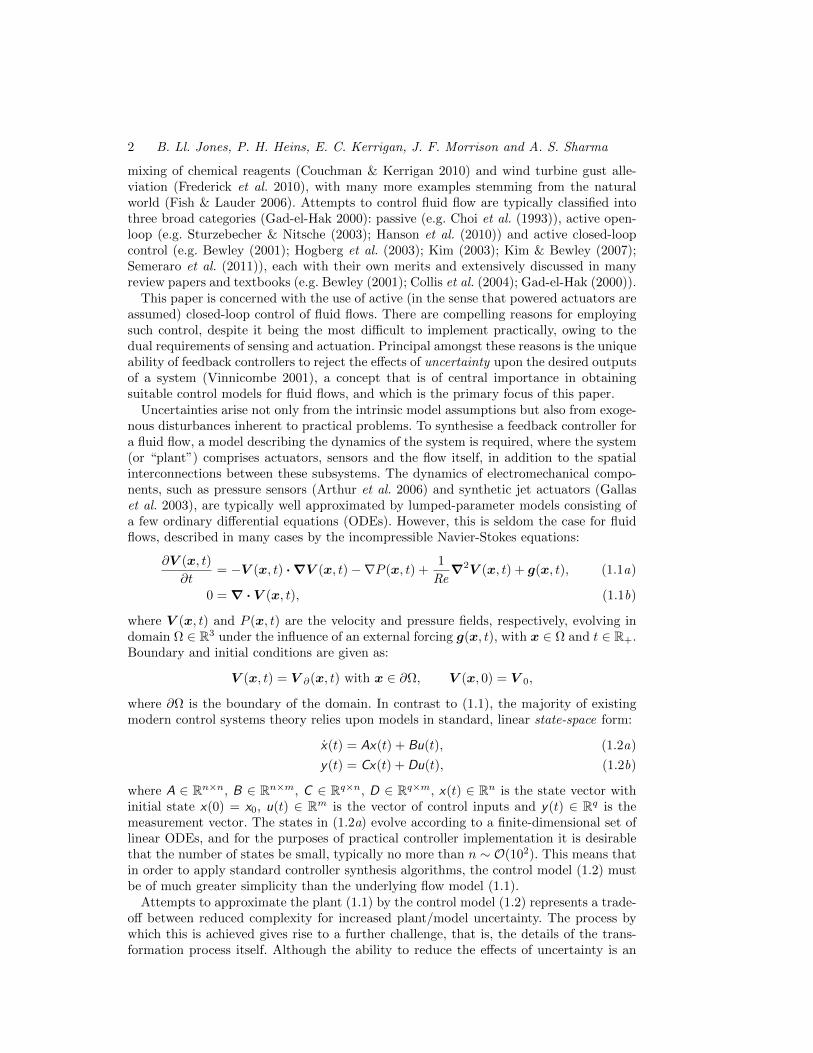
More recently McKeon & Sharma (2010); McKeon et al. (2013) explained how thestructure of turbulence and its sustainment arises from a feedback interconnection be-tween the linear and nonlinear terms of (1.1a). This is depicted in Figure 1, wherein theenergy conserving nonlinearity forces a linear subsystem that describes the dynamics offluctuations around a mean velocity profile (Sharma & McKeon 2013), with the lineardynamics playing a key role in selectively amplifying certain structures in the flow. Intheir analysis, McKeon & Sharma (2010) treated the nonlinearity of the flow arisingfrom the interaction between scales as an unstructured forcing that acts to produce aturbulent mean profile of the appropriate form. By studying the singular vectors of theresolvent operator relating this input forcing to an output velocity field, these authorswere able to predict coherent structures within the turbulent flow under study, that werein good agreement with experimental observations. The same authors also argued thatthe decomposition of the Navier-Stokes equations into a linear system driven by an un-known forcing was justifiable owing to high gain at the critical layer resulting in the linearsystem being selective to the point where the exact form of the forcing was unimportant.Sharma et al. (2011) have also proved, using the passivity theorem, that a linear feedbackcontroller can always be found to relaminarise a turbulent flow, given sufficient actuationand sensing. This was explained in physical terms with respect to Landahl’s theory ofsheared turbulence (Landahl 1977, 1975, 1967). Since the interaction of shear fluctua-

4 B. Ll. Jones, P. H. Heins, E. C. Kerrigan, J. F. Morrison and A. S. Sharma
Figure 1. System-level description of the turbulence process. The nonlinearity produces aforce f := −V · ∇V that acts as a disturbance input to the linear subsystem.
tions is linear and underpins the generation of turbulent fluctuations, the linear controlstrategy is effective. Shear interaction is a linear RDT approximation embodied in theOrr-Sommerfeld-Squire (OSS) equations: it is governed by the wall-normal disturbancevelocity which appears in the coupling term and which is related to the pressure via thelinear ‘fast’ source term in the Poisson equation for pressure fluctuations (Kim 1989;Dunn & Morrison 2003). As a result, the response to forcing of the wall-normal velocityand pressure is rather quicker than that of both the streamwise or spanwise velocities.This occurs because the shear interaction timescale is considerably shorter than eitherthe viscous or turbulence timescales (Landahl 1977) so that the Reynolds stresses areless effective. Batchelor & Townsend (1956) have shown that pressure-gradient fluctua-tions drive the momentum field, appearing as spikes in the instantaneous mean-squareacceleration. Sharma et al. (2011) have also shown that first, these fluctuations reach amaximum at y+ ≈ 20, and second, the forcing is at a maximum at the same location.This explains why the linear controller is effective even though it is operating on thewall-normal component alone. Landahl’s theory (Landahl 1975, 1967) also provides a‘wave-guide’ model of the viscous sublayer in which the least dispersive components arethose of the wall-normal velocity component and pressure fields. Clearly, understand-ing these linear mechanisms and the extent to which they are local to the wall has asignificant bearing on potential drag-reduction strategies: for active, linear control, afundamental appreciation of the shear-interaction timescale is a prerequisite and clearly,pressure is a key component to the interaction between the inner, wall region and theouter layer (Townsend 1961; Bradshaw 1967; Morrison 2007).
Given the importance of suppressing turbulence for reducing skin-friction drag, muchattention has been focussed on designing controllers for wall-bounded flows, particularlyplane channel-flows (Bewley & Liu 1998; Lee et al. 2001; Hogberg et al. 2003; Baramovet al. 2004; Hoepffner et al. 2005; Kim & Bewley 2007). Kim (2003) examined differenttypes of Linear Quadratic Regulator (LQR), also for turbulent channel flow, to minimise(1) wall-shear stress fluctuations, (2) turbulent kinetic energy, and (3), the linear couplingterm. All resulted in significant drag reduction, a common feature being a weakening ofquasi-streamwise vortices resulting in reduced high skin-friction extrema at the wall.There are many models of the near-wall cycle (see, for example, Hamilton et al. (2006))but all suggest that transient energy growth, as described by the OSS equations, providesa linear paradigm of near-wall turbulence (Butler & Farrell 1992). Central to our approachis that, for a model-based feedback controller to be successful, the role of linear dynamicscan be exploited. A key challenge is that much of our knowledge derives from directnumerical simulations at low Reynolds number (Robinson 1991) and, as a result, ourunderstanding is primarily kinematic. Here the approach is dynamic, in the sense thatany form of control implies the selective response of a flow to forcing.
We conclude this section with an acknowledgement that despite the importance oflinear mechanisms in wall-bounded turbulence, much research has also focussed on theimportance of nonlinear effects. Notable examples include the role that nonlinear mech-

Modelling for Robust Feedback Control of Fluid Flows 5
Figure 2. Robust flow control configuration, including disturbance inputs w and f arisingfrom model uncertainty and the nonlinear forcing of the flow, respectively.
anisms play in the transition process (Pringle & Kerswell 2010; Pringle et al. 2012;Cherubini et al. 2010, 2011) wherein the optimal perturbations differ considerably interms of structure and energy growth, compared to their linear counterparts.
1.2. Robust control and uncertainty in fluid flows
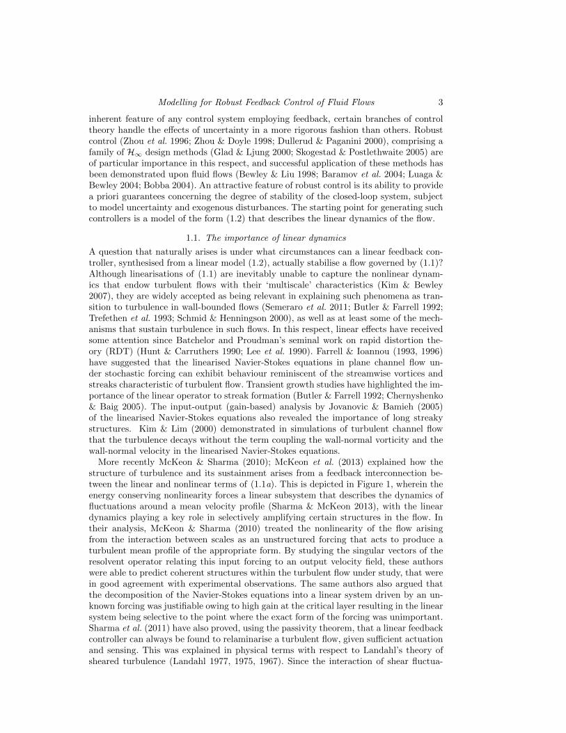
With respect to the preceding discussion, linear approximation of the flow dynamicsrepresents just one source of uncertainty between the actual flow (1.1) and state-spacemodels (1.2) employed for controller design. It is therefore important to identify andmodel the other sources of uncertainty, as such information can guide the controllerdesign process. An illustrative robust control problem is shown in Figure 2, where Kdenotes the feedback controller, U represents model uncertainty and Pgen is the nominal(approximate) model of the ‘generalised’ plant, that is, the linearised dynamical model ofthe fluid flow, the sensors and actuators, as well as the interconnection structure betweenthe plant and controller.
The generalised plant consists of individual partitions that map the control, nonlinearforcing and model uncertainty disturbance input signals, u, f and w , respectively, to themeasured output signal, y , according to:
y = Pww + Pff + Pu. (1.3a)
It is worth noting that the individual partitions are transfer function matrices, obtainablefrom a Laplace transform of a time-domain model. For example, P can be obtained fromthe Laplace transform of (1.2) as follows:
P = C (sI − A)−1B + D, (1.3b)
where s ∈ C and I is the identity matrix. The aim of the present work is to design astabilising controller K, so as to make the H∞ norm ‖·‖∞ of the closed-loop transferfunctions from w and f to y , Pyw and Pyf , respectively, both small, where:
‖Pyw‖∞ := supw 6=0
‖y(t)‖2‖w(t)‖2
, ‖Pyf‖∞ := supf 6=0
‖y(t)‖2‖f(t)‖2
. (1.3c)
Furthermore, in the interests of robustness, the controller should achieve these aims inthe presence of model uncertainty U , which represents a set of norm bounded transferfunction matrices that captures this class of uncertainty. Modelling the uncertainty setagain represents a trade-off between complexity and achievable performance, since Ushould be general enough so that the actual plant lies within the set of all perturbedplants defined by the interconnection of U with the nominal model Pgen, but not sogeneral that closed-loop performance is sacrificed. Within a flow control context, it is de-sirable that the uncertainty set U captures the discrepancy between the actual flow and a
6 B. Ll. Jones, P. H. Heins, E. C. Kerrigan, J. F. Morrison and A. S. Sharma
simpler control model. Bobba (2004) was amongst the first to categorise the uncertaintythat arises when approximating (1.1) by a model in linear, state-space form (1.2). Thesesources of uncertainty are summarised as follows:
• Model uncertainty. This takes two forms. The first of these is parametric uncer-tainty that arises owing to a lack of precise knowledge of the parameters (e.g. Reynoldsnumber) of the system. Also, if the governing equations are linearised around an equi-librium flow solution, then the theoretical and actual mean flows may differ. Anothersource of parametric error might arise from numerical errors incurred during the processof eliminating the algebraic constraint (1.1b) to obtain an unconstrained system (1.2a).This arises, for example, when inverting an ill-conditioned discretised Laplacian to ob-tain the Orr-Sommerfeld matrix. Secondly, dynamic uncertainty, which is inherent inany finite-dimensional approximation of an infinite-dimensional system. Spatial discreti-sations of (1.1) only resolve a finite number of dynamic modes, typically those of low-est spatial frequency, and consequently neglect all higher frequency modes. Of thosemodes that are retained by a spatial discretisation, some will be better resolved thanothers (Boyd 2001). The problem of determining a suitable level of spatial refinement(and hence which modes are of dynamical importance) is of fundamental importance indesigning controllers that can tolerate the uncertainty arising from the use of a finite-dimensional flow model. Addressing this issue is an important contribution of this paper.• Disturbance uncertainty. In practice, a flow will be subjected to disturbances arising
from a number of sources, such as uncertain boundary conditions, forcing from acousticnoise and the coupling of sensor noise into the flow via a feedback controller. Such dis-turbances may be impractical to model in any great detail, other than perhaps knowinga bound on their magnitude and the point at which they enter the closed-loop system. Inaddition, and as discussed in Section 1.1, the nonlinearity of the Navier-Stokes equationscan be treated as an uncertain disturbance forcing acting upon the linear system. From acontrol systems perspective this is important, since it enables the problem of suppressingturbulence to be formulated as a disturbance rejection problem.
In summary, in order for a feedback controller to guarantee robustness to these sourcesof model uncertainty, the controller design process must account for each uncertainty insome way. The manner in which this can be achieved is discussed in the following section.
1.3. Addressing sources of uncertainty
If bounds on all the uncertainties listed above are known, then each uncertainty can be‘extracted’ from the plant model to form a structured perturbation matrix U , and thisstructure can then be exploited in subsequent controller designs, based on structured-singular-value synthesis algorithms (Skogestad & Postlethwaite 2005). An alternative,and simpler class of uncertainty model exists in the form of unstructured uncertainty,whereby the perturbation matrix U is ‘full’. Many different unstructured uncertaintymodels exist (Vinnicombe 2001), such as additive uncertainty, multiplicative input un-certainty and inverse multiplicative output uncertainty, each with their own merits interms of representing parametric, dynamic and disturbance uncertainty. An appropriateuncertainty model for closed-loop flow control, for reasons that will be discussed below,is that of coprime factor uncertainty. Background material on this subject is presentedin Appendix A, but we note, briefly, that coprime factor perturbations take the form:
Pp :=
(N + UN )(M+ UM)−1, (1.4)

Modelling for Robust Feedback Control of Fluid Flows 7
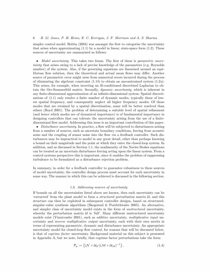
Figure 3. Feedback control diagram for disturbance rejection. The objective is to design theloop-shaping controller K to reject the disturbance, arising form the nonlinear forcing f , uponthe measured outputs y (e.g. wall shear-stress) of the flow system. The system within the shadedregion is the closed-loop transfer function matrix Pyf (1.5) from disturbance forcing to output.
where the nominal plant P := NM−1 is separated into its stable coprime factors Nand M, each of which are perturbed by norm bounded perturbations UN , and UM,respectively, to form a set of perturbed plants Pp.
Although seemingly abstract, this class of uncertainty is particularly useful as it can beregarded as a blend of multiplicative and inverse multiplicative type uncertainties thatnaturally account for dynamic and parametric uncertainty, respectively (Vinnicombe2001). It also accounts for uncertainty in the number of right-half plane system polesand zeroes, both of which impose fundamental performance limitations upon feedbackcontrollers. It is worth emphasising that the use of such an unstructured uncertaintydescription greatly reduces the difficulty of modelling the uncertainty set, and hencereduces the difficulty of designing a robust controller. Indeed, in the case of coprimefactor uncertainty, no effort is required at all since controller synthesis techniques thatemploy this description, such as the H∞ loop-shaping procedure of McFarlane & Glover(1992), automatically synthesise controllers that maximise the amount of coprime factoruncertainty that a closed-loop system can tolerate. In doing so, and as explained furtherin Appendix A, H∞ loop-shaping controllers also attenuate the effect of disturbancesentering at different points in the system (including sensor noise). To see this is the casefor rejecting the influence of the forcing arising from the nonlinearity of the flow, consideragain the system described by the model (1.3a). Assuming an output feedback controllaw of the form u = −Ky leads to the following expression for the closed-loop transferfunction Pyf that relates f to y :
y = (I + PK)−1 Pf︸ ︷︷ ︸
Pyf
f . (1.5)
The relevant closed-loop system is depicted in Figure 3. The control objective is to re-duce the influence of f upon y , and this is achieved by making the gain of Pyf small (interms of ‖Pyf‖∞), which in turn amounts to designing the loop-shaping controller K toensure that the gain of the open-loop system PK is greater than unity, as can be seenfrom inspection of (1.5). Such loop-shaping controllers therefore provide a convenientframework for dealing with the parametric, dynamic and disturbance uncertainties en-countered when attempting to control flows (1.1) from controllers designed upon simplermodels (1.2). This simplicity of designing robust controllers has thus meant that H∞loop-shaping controllers have found use in a variety of applications, ranging from theflight control of vertical take-off aircraft (Hyde et al. 1995), control of combustion os-cillations (Chu et al. 2003), bluff body form-drag reduction (Dahan et al. 2012) andwind-turbine active blade-pitch control (Lu et al. 2014).
Of the many studies conducted into feedback control of wall-bounded flows, few have
8 B. Ll. Jones, P. H. Heins, E. C. Kerrigan, J. F. Morrison and A. S. Sharma
explicitly addressed the issue of uncertainty modelling with respect to the class of uncer-tainties listed above. This is not to say that such feedback controllers have not been robust(at least to some extent), but such assessment has only been possible after closed-looptesting, rather than at the controller design stage. The focus of this paper, therefore, isupon obtaining state-space models (1.2) of flows described by linearisations of (1.1), thatare of sufficient simplicity to enable straightforward synthesis of controllers with a prioristability and performance guarantees.
The remainder of this paper is organised as follows. We begin in Section 2 by formulat-ing the modelling problem. The starting point is the linearised Navier-Stokes equationsand the finishing point is a low-order, state-space model suitable for controller synthesis.On the way we show how to numerically convert a system of DAEs to one of ODEs, andthe motivation for doing so. We also introduce the ν-gap metric as a useful tool fromfeedback control theory and show how it can be used to efficiently derive low-order state-space models from spatial discretisations of the linearised flow system. In Section 3, aH∞loop-shaping controller is designed from a low-order model and applied to plane channel-flow. Significant portions of this paper are expository in nature and assume little priorknowledge from the reader of feedback control, other than a rudimentary appreciation ofclassical loop-shaping techniques such as PID control and lead/lag compensation (Astrom& Murray 2008). To preserve clarity of exposition, some control systems material is in-cluded as appendices. In particular, background material on coprime-factor uncertaintyand H∞-loop shaping is presented, as are the algorithms employed to firstly convert thesemi-discretised Navier-Stokes equations into a standard state-space model.
2. Formulation of low-order control models
The dynamics of infinitesimal perturbations in a viscous, incompressible, wall-boundedflow can be described by linearisation of the Navier-Stokes equations (1.1) around a meanflow solution. Subsequent spatial discretisation yields a system in the generalised state-space (or descriptor) form:[
E11 00 0
]︸ ︷︷ ︸
ED
d
dt
[v(t)p(t)
]︸ ︷︷ ︸
xD(t)
=
[A11 A12
A21 0
]︸ ︷︷ ︸
AD
[v(t)p(t)
]︸ ︷︷ ︸xD(t)
+
[B1
B2
]︸ ︷︷ ︸BD
u(t), (2.1)
where v(t) ∈ Cnv and p(t) ∈ Cnp are the semi-discretised vectors of (perturbation)velocities and pressure, respectively, and u(t) ∈ Cm is a vector of control inputs. Thestate vector is xD(t), E11 ∈ Cnv×nv is the symmetric, positive definite mass matrixand A11 ∈ Cnv×nv contains a mixture of discrete diffusion and linearised convectiveterms. The matrices A12 ∈ Cnv×np and A21 ∈ Cnp×nv represent the discrete gradientand divergence operators, respectively, and B1 ∈ Cnv×m and B2 ∈ Cnp×m describe howthe control inputs influence the states. Note that the subscript ‘D’, denotes vectors andmatrices pertaining to descriptor state-space systems.
The state evolution equation (2.1), together with the measurement equation y(t) =CDxD(t) + DDu(t), can be written as a descriptor state-space system:
EDxD(t) = ADxD(t) + BDu(t), (2.2a)
y(t) = CDxD(t) + DDu(t), (2.2b)
where ED, AD ∈ CnD×nD , CD ∈ Cq×nD , DD ∈ Cq×m and y(t) ∈ Cq is the vector ofmeasured outputs. The order nD = nv +np of the state vector depends on the resolution,but is typically very large for simulation models (e.g. nD > 106). For control models,

Modelling for Robust Feedback Control of Fluid Flows 9
Figure 4. Side view of plane channel flow and conceptual sketch of the control system. Spatiallycontinuous actuation (transpiration) and sensing (streamwise shear stress) occurs at both walls.For a given wavenumber pair, the feedback controller K takes, as inputs, the sensor measure-ments y , and outputs a control signal u to the actuators.
however, the number of states need not be the same, and can in fact be much lower, asdiscussed in more detail in Section 2.3.
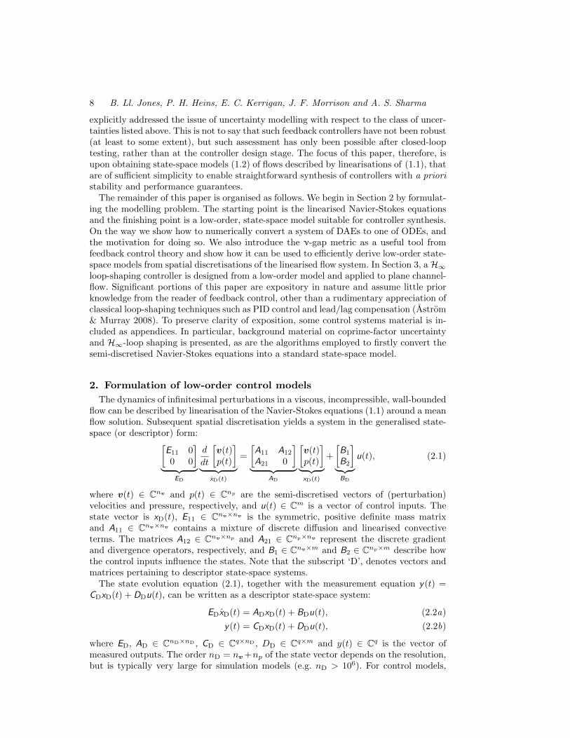
As an example of the above formulation, consider the fully developed flow betweentwo infinite, parallel, planar and stationary boundaries, as shown in Figure 4. Non-dimensionalising length scales by the channel half-height, h, velocities by the centre-linevelocity Ucl and pressure by ρU2
cl, the linearised Navier-Stokes equations for incompress-ible plane channel flow are (Aamo & Krstic 2003; McKernan 2006):
∂u
∂t= −U ∂u
∂x− v ∂U
∂y− ∂p
∂x+
1
Re∇2u, (2.3a)
∂v
∂t= −U ∂v
∂x− ∂p
∂y+
1
Re∇2v, (2.3b)
∂w
∂t= −U ∂w
∂x− ∂p
∂z+
1
Re∇2w, (2.3c)
0 =∂u
∂x+∂v
∂y+∂w
∂z, (2.3d)
where Re = ρUclh/µ is the Reynolds number and the mean velocity profile satisfiesU = 1 − y2. In non-dimensional co-ordinates the upper and lower walls are located aty = ±1. The streamwise, wall-normal and spanwise perturbation velocities u, v and w,respectively, and perturbation pressure p are functions of x, y, z and t . The initial andboundary conditions are as follows:
u(x, y, z, 0) = u0, v(x, y, z, 0) = v0, w(x, y, z, 0) = w0, (2.4a)
u(x,±1, z, t) = 0, v(x,±1, z, t) = 0, w(x,±1, z, t) = 0. (2.4b)
For the purposes of the current investigation, it is sufficient to employ actuators andsensors that render the system (2.3) controllable and observable (Astrom & Murray 2008;Bewley & Liu 1998). Therefore, the walls are assumed continuously distributed with walltranspiration actuators and sensors capable of measuring the streamwise component ofthe wall-shear stress (Aamo & Krstic 2003; Bewley & Liu 1998; McKernan et al. 2006).A conceptual sketch of this arrangement is shown in Figure 4. The control objective ofthe present study is to attenuate the streamwise wall-shear stress perturbations. Sucha control objective was employed by Lee et al. (2001) and Lim (2003), where linearcontrollers were synthesised that significantly reduced the wall-shear stress perturbations,leading to significant reductions in the mean drag.

10 B. Ll. Jones, P. H. Heins, E. C. Kerrigan, J. F. Morrison and A. S. Sharma
Actuator dynamics are accounted for by modelling the dynamics of the actuationsurfaces as first-order systems with a time constant ς ∈ R. For effective control, theactuators should possess sufficient bandwidth to counter the disturbances within theflow. For the present study, a value of ς = 1 was found sufficient. Assuming the controlinputs u(x, y, z, t) are voltages supplied to each actuation surface, then the control inputcan be modelled by the following inhomogenous boundary conditions on the upper andlower walls, respectively:
∂v(x,+1, z, t)
∂t:= −1
ςv(x,+1, z, t) +
1
ςu(x,+1, z, t), (2.5a)
∂v(x,−1, z, t)
∂t:= −1
ςv(x,−1, z, t) +
1
ςu(x,−1, z, t). (2.5b)
In terms of measurements we consider the streamwise component of the wall shearstress τxy at both walls:
y(x, y, z, t) :=
[τyx|y=+1
τyx|y=−1
]=
1
Re
(∂u∂y + ∂v∂x
)∣∣y=+1(
∂u∂y + ∂v
∂x
)∣∣y=−1
. (2.6)
Having defined inputs and outputs, the infinite-dimensional system (2.3) is then renderedfinite-dimensional via spatial discretisation. The flow is Fourier-transformed in the spa-tially homogenous x and z directions, in which case the distributed control input u isapproximated as follows:
u(x,±1, z, t) ≈ R
(Nx∑
nx=1
Nz∑nz=1
u(±1, t)ei(αx+βz)
), (2.7)
where i :=√−1, α and β are streamwise and spanwise wavenumbers, respectively,
and u ∈ C2 are the Fourier-transformed inputs at each wavenumber pair (α, β). Theoutput equation (2.6) is similarly approximated. In the inhomogenous y direction theflow is discretised on Ny Chebyshev collocation nodes (Weideman & Reddy 2000) and
the spatial y-derivatives ∂∂y ,
∂2
∂y2 are approximated by Chebyshev differentiation ma-
trices Ych, Y 2ch, respectively (Weideman & Reddy 2000). Application of the Fourier-
transform decouples the system dynamics by wavenumber, and so the flow dynamics foreach individual pair (α, β) can now be expressed as a linear, finite-dimensional descriptorstate-space system:
ED11 0 0 00 ED22 0 00 0 ED33
00 0 0 0
︸ ︷︷ ︸
ED
d
dt
uny (t)vny (t)wny (t)pny (t)
︸ ︷︷ ︸
xD(t)
=
AD11 AD12 0 AD14
0 AD22 0 AD24
0 0 AD33AD34
AD41AD42
AD430
︸ ︷︷ ︸
AD
uny (t)vny (t)wny (t)pny (t)
︸ ︷︷ ︸xD(t)
+
0 0
BD21BD22
0 00 0
︸ ︷︷ ︸
BD
u(t),
(2.8a)
y(t) =
[CD11
CD120 0
CD21 CD22 0 0
]︸ ︷︷ ︸
CD
xD(t), (2.8b)
where uny (t), vny (t), wny (t) and pny (t) are vectors containing the Fourier transformedvelocity and pressure coefficients at the ny-th collocation node (where 1 6 ny 6 Ny) fora given wavenumber pair. The elements of the dynamics matrix are defined as: AD11
:=

Modelling for Robust Feedback Control of Fluid Flows 11
AD22 := AD33 := −iαUny + 1
Re ∆, AD12:= −dUny
dy , AD14 := −AD41 := −αI , AD24 :=−AD42
:= −Ych, AD34:= −AD43
:= −βI , and ED11:= ED22
:= ED33:= I , where i :=√
−1, Uny := 1 − y2ny and ∆ := −α2 + Y 2ch − β2 is the discrete Laplacian operator. The
control input influences the states via BD21 := [ 1ς 0 ... 0 ]
Tand BD22 :=[ 0 ... 0 1
ς ]T
. In thecase of streamwise shear-stress measurements CD11
:= 1
Re Ych 1,1:Ny(1/Re times the top
row of Ych), CD12:= 1
Re [ iα 0 ... 0 ], CD21:= 1
Re Ych Ny,1:Ny, and CD22
:= 1
Re [ 0 ... 0 iα ].
Boundary conditions (2.4b)–(2.5b) are enforced in a straightforward fashion by modifyingthe top and bottom rows of the submatrices in ED and AD. For example, the no slipcondition u(x,+1, z, t) = 0 is enforced by setting the top rows of ED11
, AD11, AD12
and AD14 equal to zero, except for the (1, 1) element of AD11 which is set equal to 1,whist (2.5a) is satisfied by setting the top rows of AD22 and AD24 to zero, with theexception of the (1, 1) element of AD22
, which is set to −1/ς.
2.1. Dealing with descriptor systems: Eliminating the incompressibility constraint
Control of descriptor state-space systems (2.2) is less well understood than that for stan-dard state-space systems (1.2), and so controller synthesis becomes more straightforwardif the former can be converted into the latter. This is trivial when the inverse of ED ex-ists, since both sides of (2.2a) can be premultiplied by E−1D . However, this is not possiblein (2.1) since ED is singular, owing to the assumption of incompressibility. To overcomethis difficulty, the system (2.3) is usually reformulated so that the resulting ED matrix isnon-singular and can be inverted to yield a standard state-space system. For the case ofplane channel flow, it is possible to analytically eliminate the divergence constraint (2.3d)by reformulating the system in terms of a divergence-free basis described in terms of wall-normal velocities and wall-normal vorticities. A non-singular ED can then be obtained byusing a set of basis functions that individually satisfy the boundary conditions, yieldingthe familiar OSS system (Schmid & Henningson 2000; Kim & Lim 2000):
d
dt
[vny (t)
ζny (t)
]=
[LOS 0LC LS
]︸ ︷︷ ︸
AOSS
[vny (t)
ζny (t)
], (2.9a)
where ζny (t) is the vector of Fourier transformed wall-normal vorticities at a particularwavenumber pair. The OSS matrix AOSS consists of the Orr-Sommerfeld matrix LOS, theCoupling matrix LC and the Squire matrix LS:
LOS := ∆−1(−iαUny∆ + iα
d2Uny
dy2+
1
Re∆2
), (2.9b)
LC := −iβdUny
dy, (2.9c)
LS := −iαUny +1
Re∆, (2.9d)
Although this reformulation has proven itself invaluable for hydrodynamic stabilityanalyses, its use for control system design is not without limitation. For instance, it isdifficult to analytically obtain divergence-free bases for more complicated flows, suchas those with variable fluid properties, or those with complex geometries (Ferziger &Peric 1997). This is one of the main reasons why the majority of feedback flows controlstudies have concentrated on channel flows or similar, parallel, shear flows. Also, satisfyingboundary conditions in a divergence-free basis is considerably more difficult than inthe original primitive-variable basis, particularly for complex geometries. The boundary
12 B. Ll. Jones, P. H. Heins, E. C. Kerrigan, J. F. Morrison and A. S. Sharma
conditions, naturally expressed in terms of primitive variables, must be transformedto equivalent conditions in a divergence-free basis that is subject to higher-order spatialderivatives (e.g. fourth-order in (2.9b)). Failure to satisfy these conditions precisely resultsin an unphysical system, contaminated by ‘spurious’ eigenmodes (Bewley & Liu 1998).
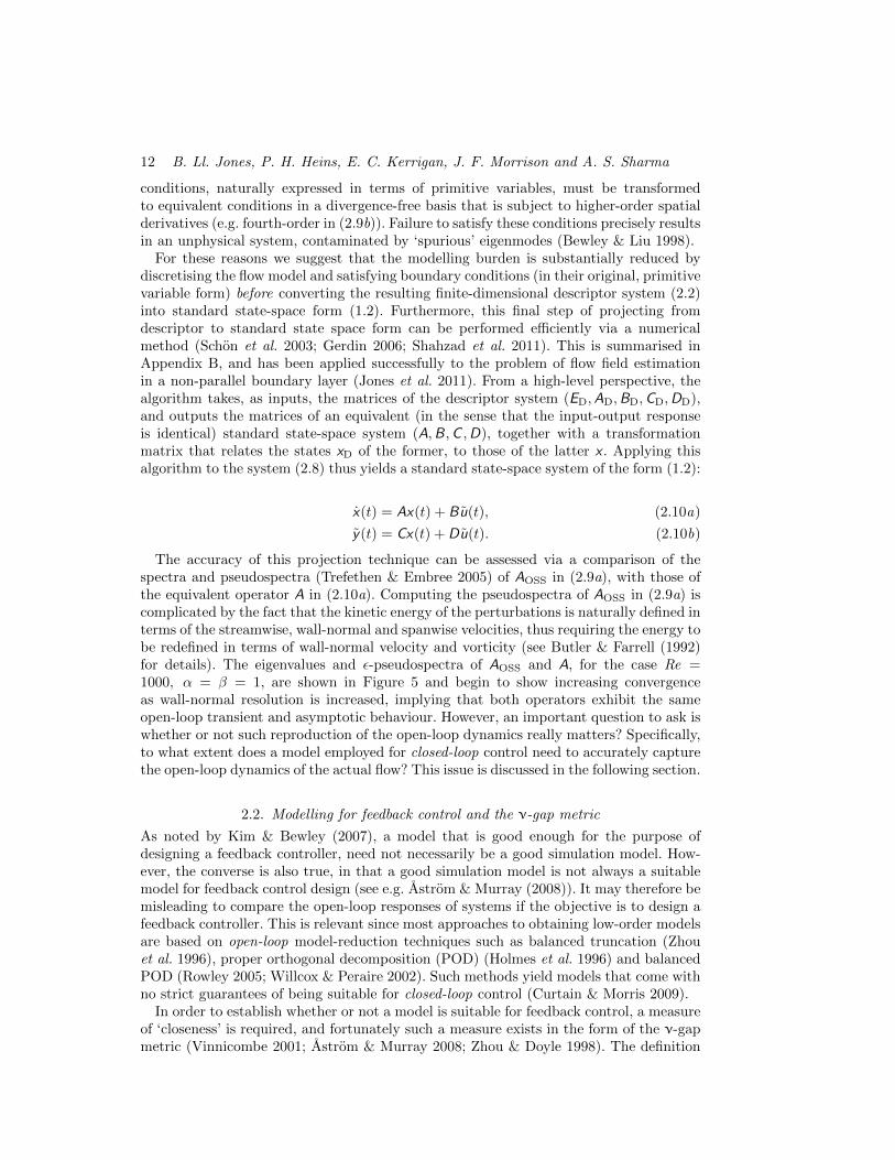
For these reasons we suggest that the modelling burden is substantially reduced bydiscretising the flow model and satisfying boundary conditions (in their original, primitivevariable form) before converting the resulting finite-dimensional descriptor system (2.2)into standard state-space form (1.2). Furthermore, this final step of projecting fromdescriptor to standard state space form can be performed efficiently via a numericalmethod (Schon et al. 2003; Gerdin 2006; Shahzad et al. 2011). This is summarised inAppendix B, and has been applied successfully to the problem of flow field estimationin a non-parallel boundary layer (Jones et al. 2011). From a high-level perspective, thealgorithm takes, as inputs, the matrices of the descriptor system (ED,AD,BD,CD,DD),and outputs the matrices of an equivalent (in the sense that the input-output responseis identical) standard state-space system (A,B,C ,D), together with a transformationmatrix that relates the states xD of the former, to those of the latter x . Applying thisalgorithm to the system (2.8) thus yields a standard state-space system of the form (1.2):
x(t) = Ax(t) + Bu(t), (2.10a)
y(t) = Cx(t) + Du(t). (2.10b)
The accuracy of this projection technique can be assessed via a comparison of thespectra and pseudospectra (Trefethen & Embree 2005) of AOSS in (2.9a), with those ofthe equivalent operator A in (2.10a). Computing the pseudospectra of AOSS in (2.9a) iscomplicated by the fact that the kinetic energy of the perturbations is naturally defined interms of the streamwise, wall-normal and spanwise velocities, thus requiring the energy tobe redefined in terms of wall-normal velocity and vorticity (see Butler & Farrell (1992)for details). The eigenvalues and ε-pseudospectra of AOSS and A, for the case Re =1000, α = β = 1, are shown in Figure 5 and begin to show increasing convergenceas wall-normal resolution is increased, implying that both operators exhibit the sameopen-loop transient and asymptotic behaviour. However, an important question to ask iswhether or not such reproduction of the open-loop dynamics really matters? Specifically,to what extent does a model employed for closed-loop control need to accurately capturethe open-loop dynamics of the actual flow? This issue is discussed in the following section.
2.2. Modelling for feedback control and the ν-gap metric
As noted by Kim & Bewley (2007), a model that is good enough for the purpose ofdesigning a feedback controller, need not necessarily be a good simulation model. How-ever, the converse is also true, in that a good simulation model is not always a suitablemodel for feedback control design (see e.g. Astrom & Murray (2008)). It may therefore bemisleading to compare the open-loop responses of systems if the objective is to design afeedback controller. This is relevant since most approaches to obtaining low-order modelsare based on open-loop model-reduction techniques such as balanced truncation (Zhouet al. 1996), proper orthogonal decomposition (POD) (Holmes et al. 1996) and balancedPOD (Rowley 2005; Willcox & Peraire 2002). Such methods yield models that come withno strict guarantees of being suitable for closed-loop control (Curtain & Morris 2009).
In order to establish whether or not a model is suitable for feedback control, a measureof ‘closeness’ is required, and fortunately such a measure exists in the form of the ν-gapmetric (Vinnicombe 2001; Astrom & Murray 2008; Zhou & Doyle 1998). The definition

Modelling for Robust Feedback Control of Fluid Flows 13
Figure 5. Eigenvalues (dots) and ε-pseudospectra (contours) in lower-left quadrant of the com-plex plane for (a), (b) AOSS in (2.9a), and (c), (d) A in (2.10a). Pseudospectral contours plottedfor ε = 10−3.5, 10−3, . . . , 10−2 (outermost contour). Left plots are computed for low wall-normalresolution (Ny = 20 grid-points), right plots are for higher resolution (Ny = 40). Computedvalues are for Reynolds number Re = 103 and wavenumbers α = β = 1. Also shown are thevalues of the eigenvalues with maximum real part λmax, corresponding to those eigenmodes thatare least stable in the sense that their eigenvalues are closest to the right-half of the complexplane.
of the ν-gap metric is beyond the scope of the present work, but it suffices to state thatthe ν-gap between two systems, denoted δν(Pa,Pb), is a metric and thus satisfies thefollowing important properties:
0 6 δν(Pa,Pb) 6 1, (2.11a)
δν(Pa,Pc) 6 δν(Pa,Pb) + δν(Pb,Pc) (Triangle inequality). (2.11b)
The ν-gap assumes systems are connected in feedback by a unity gain controller (K = I ).This is a restrictive assumption, but is easily overcome by shaping the systems withcompensators, as in Figure 6, that are designed to shape the open-loop system in adesirable fashion (e.g. high gain at low frequencies, low gain at high frequencies, etc.) ina similar manner to classical control methods, such as PID or lag-lead control. The ν-gap is then computed between the shaped systems δν(Pa,W ,Pb,W). Thus, the ν-gap isvery much dependent on the closed-loop objectives encapsulated by the compensatorfunctions. This is important since determining whether or not a model is suitable fordesigning feedback controllers depends not just on the nominal system, but also uponthe closed-loop control objectives. Lastly, the ν-gap metric is of considerable practical
14 B. Ll. Jones, P. H. Heins, E. C. Kerrigan, J. F. Morrison and A. S. Sharma
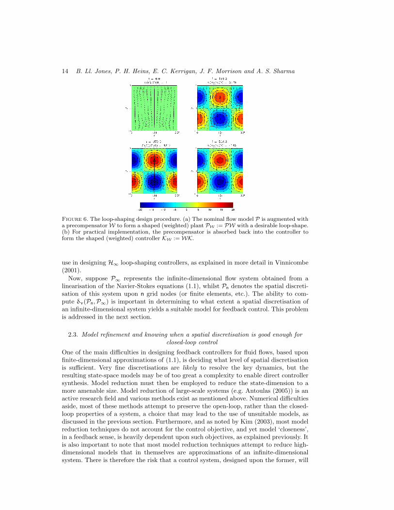
Figure 6. The loop-shaping design procedure. (a) The nominal flow model P is augmented witha precompensatorW to form a shaped (weighted) plant PW := PW with a desirable loop-shape.(b) For practical implementation, the precompensator is absorbed back into the controller toform the shaped (weighted) controller KW :=WK.
use in designing H∞ loop-shaping controllers, as explained in more detail in Vinnicombe(2001).
Now, suppose P∞ represents the infinite-dimensional flow system obtained from alinearisation of the Navier-Stokes equations (1.1), whilst Pn denotes the spatial discreti-sation of this system upon n grid nodes (or finite elements, etc.). The ability to com-pute δν(Pn,P∞) is important in determining to what extent a spatial discretisation ofan infinite-dimensional system yields a suitable model for feedback control. This problemis addressed in the next section.
2.3. Model refinement and knowing when a spatial discretisation is good enough forclosed-loop control
One of the main difficulties in designing feedback controllers for fluid flows, based uponfinite-dimensional approximations of (1.1), is deciding what level of spatial discretisationis sufficient. Very fine discretisations are likely to resolve the key dynamics, but theresulting state-space models may be of too great a complexity to enable direct controllersynthesis. Model reduction must then be employed to reduce the state-dimension to amore amenable size. Model reduction of large-scale systems (e.g. Antoulas (2005)) is anactive research field and various methods exist as mentioned above. Numerical difficultiesaside, most of these methods attempt to preserve the open-loop, rather than the closed-loop properties of a system, a choice that may lead to the use of unsuitable models, asdiscussed in the previous section. Furthermore, and as noted by Kim (2003), most modelreduction techniques do not account for the control objective, and yet model ‘closeness’,in a feedback sense, is heavily dependent upon such objectives, as explained previously. Itis also important to note that most model reduction techniques attempt to reduce high-dimensional models that in themselves are approximations of an infinite-dimensionalsystem. There is therefore the risk that a control system, designed upon the former, will
Modelling for Robust Feedback Control of Fluid Flows 15
fail to stabilise the latter, owing to a phenomenon known as ‘spillover’ (Balas 1978),whereby a controller excites unmodelled plant dynamics.
Jones & Kerrigan (2010) developed an alternative method for obtaining low-ordercontrol models of spatially distributed systems, that circumvented each of the problemsdescribed above. The method involved computing a sequence of ν-gaps between low-orderplant-models of successively finer spatial resolution, starting from a coarsely discretised(and thus low-order) model. This gradual refinement of model resolution is the conceptualopposite of model reduction-based approaches, and can hence be thought of as modelrefinement. Generally speaking, as spatial resolution is increased, the sequence of ν-gapsbetween successive plant-models asymptotes towards zero, reflecting the fact that froma closed-loop perspective there are diminishing returns to be obtained from employinghighly resolved models. The rate at which the sequence converges to zero is dependentupon the flow, the control objective and the method of spatial discretisation, but canbe very great. Establishing the rate of convergence enables the construction of an upperbound on the ν-gap between the models in the computed sequence and the infinitedimensional plant, which then informs the selection of a suitable low-order model (Jones& Kerrigan 2010). This enables the synthesis, on low-order models, of robust controllersthat are guaranteed to stabilise the actual plant, a feature not shared by model reductionmethods where the gap between the high-order model (e.g. a DNS flow model) andplant (e.g. Navier-Stokes equations) is not known, and where the gap between high-order and reduced models may be too expensive to compute. Since the calculation ofthe bound is based on shaped plant-models of small state-dimension, model refinementavoids the numerical problems inherent in large-scale model reduction-based approaches.Its application here is the first that we are aware of upon a flow control problem.
The design procedure is summarised as follows. Firstly, closed-loop objectives are spec-ified by the construction of a precompensator to form the weighted (infinite-dimensional)plant P∞,W . This is then discretised on an initial grid of ni nodes (where ni is small),using an appropriate means of spatial discretisation (finite-difference, finite-element,spectral, etc.), producing a low-order, finite-dimensional plant model Pni,W . Ideally,one would compute δν(Pni,W ,P∞,W) directly, but in general this is not possible. How-ever, it is straightforward to form an upper bound as follows. Starting from n = ni,compute the ν-gaps between models of successively finer discretisation to form a se-quence δν(Pn,W ,Pn+1,W) and stop when this sequence begins to asymptote towardszero, at some number of grid points n = n0. Then construct a sequence an with afinite series (such as a geometric progression) that upper bounds the ν-gap sequence forall n > n0. The triangle inequality property of the ν-gap metric (2.11b) can then beexploited as follows:
δν(Pn0,W ,P∞,W) 6∞∑
n=n0
δν(Pn,W ,Pn+1,W) 6∞∑
n=n0
an. (2.12)
Thus, the ν-gap between the low-order, finite dimensional plant-model Pn0,W and theinfinite-dimensional plant P∞,W can be bounded by computing the series of the se-quence an. Then, provided the robust stability margin of a H∞ loop-shaping controller(synthesised from Pn0,W) exceeds this bound by a reasonable margin, then robust closed-loop performance is guaranteed. The assumptions and technical details underpinning thisprocess are fully discussed in Jones & Kerrigan (2010), and a sketch of the procedure isshown in Figure 7.
The model refinement method embodies the fact that sensibly designed feedback con-trol systems are insensitive to unmodelled dynamics occurring at frequencies above the
16 B. Ll. Jones, P. H. Heins, E. C. Kerrigan, J. F. Morrison and A. S. Sharma
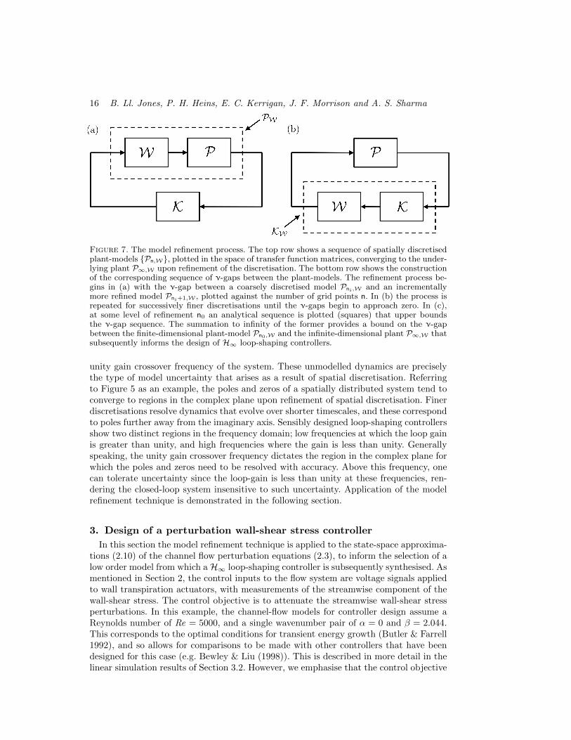
Figure 7. The model refinement process. The top row shows a sequence of spatially discretisedplant-models Pn,W, plotted in the space of transfer function matrices, converging to the under-lying plant P∞,W upon refinement of the discretisation. The bottom row shows the constructionof the corresponding sequence of ν-gaps between the plant-models. The refinement process be-gins in (a) with the ν-gap between a coarsely discretised model Pni,W and an incrementallymore refined model Pni+1,W , plotted against the number of grid points n. In (b) the process isrepeated for successively finer discretisations until the ν-gaps begin to approach zero. In (c),at some level of refinement n0 an analytical sequence is plotted (squares) that upper boundsthe ν-gap sequence. The summation to infinity of the former provides a bound on the ν-gapbetween the finite-dimensional plant-model Pn0,W and the infinite-dimensional plant P∞,W thatsubsequently informs the design of H∞ loop-shaping controllers.
unity gain crossover frequency of the system. These unmodelled dynamics are preciselythe type of model uncertainty that arises as a result of spatial discretisation. Referringto Figure 5 as an example, the poles and zeros of a spatially distributed system tend toconverge to regions in the complex plane upon refinement of spatial discretisation. Finerdiscretisations resolve dynamics that evolve over shorter timescales, and these correspondto poles further away from the imaginary axis. Sensibly designed loop-shaping controllersshow two distinct regions in the frequency domain; low frequencies at which the loop gainis greater than unity, and high frequencies where the gain is less than unity. Generallyspeaking, the unity gain crossover frequency dictates the region in the complex plane forwhich the poles and zeros need to be resolved with accuracy. Above this frequency, onecan tolerate uncertainty since the loop-gain is less than unity at these frequencies, ren-dering the closed-loop system insensitive to such uncertainty. Application of the modelrefinement technique is demonstrated in the following section.
3. Design of a perturbation wall-shear stress controller
In this section the model refinement technique is applied to the state-space approxima-tions (2.10) of the channel flow perturbation equations (2.3), to inform the selection of alow order model from which aH∞ loop-shaping controller is subsequently synthesised. Asmentioned in Section 2, the control inputs to the flow system are voltage signals appliedto wall transpiration actuators, with measurements of the streamwise component of thewall-shear stress. The control objective is to attenuate the streamwise wall-shear stressperturbations. In this example, the channel-flow models for controller design assume aReynolds number of Re = 5000, and a single wavenumber pair of α = 0 and β = 2.044.This corresponds to the optimal conditions for transient energy growth (Butler & Farrell1992), and so allows for comparisons to be made with other controllers that have beendesigned for this case (e.g. Bewley & Liu (1998)). This is described in more detail in thelinear simulation results of Section 3.2. However, we emphasise that the control objective
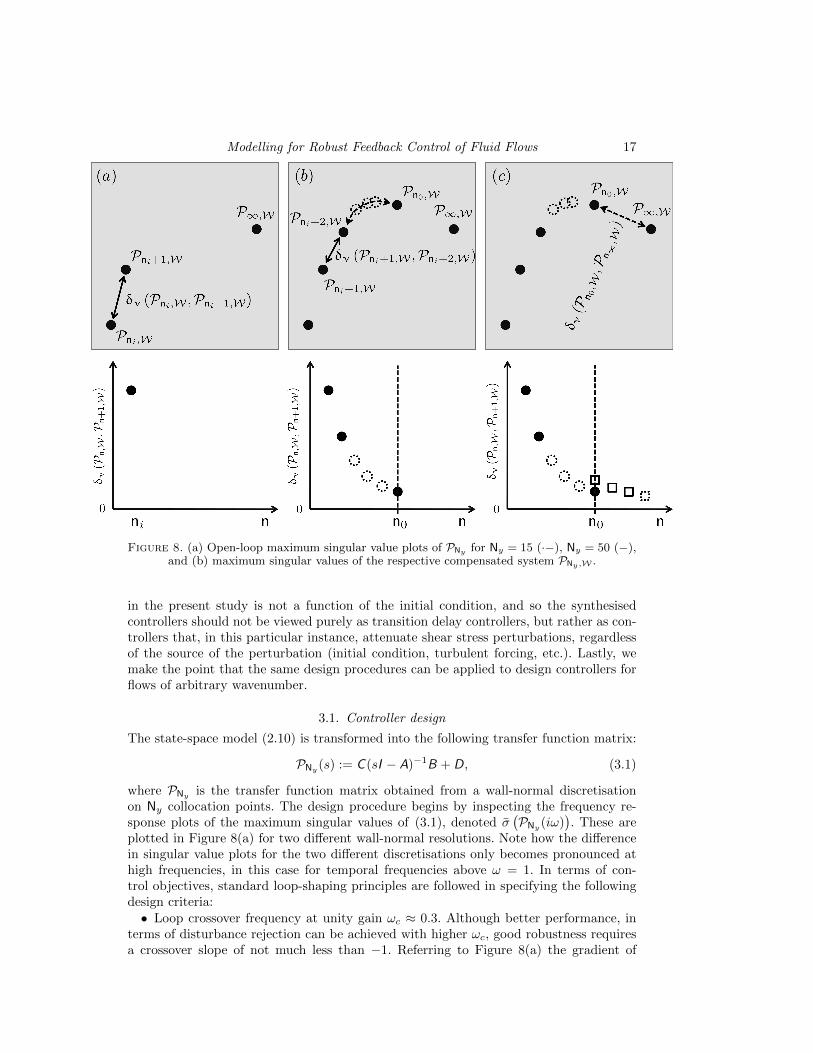
Modelling for Robust Feedback Control of Fluid Flows 17
Figure 8. (a) Open-loop maximum singular value plots of PNy for Ny = 15 (·−), Ny = 50 (−),and (b) maximum singular values of the respective compensated system PNy,W .
in the present study is not a function of the initial condition, and so the synthesisedcontrollers should not be viewed purely as transition delay controllers, but rather as con-trollers that, in this particular instance, attenuate shear stress perturbations, regardlessof the source of the perturbation (initial condition, turbulent forcing, etc.). Lastly, wemake the point that the same design procedures can be applied to design controllers forflows of arbitrary wavenumber.
3.1. Controller design
The state-space model (2.10) is transformed into the following transfer function matrix:
PNy (s) := C (sI − A)−1B + D, (3.1)
where PNyis the transfer function matrix obtained from a wall-normal discretisation
on Ny collocation points. The design procedure begins by inspecting the frequency re-sponse plots of the maximum singular values of (3.1), denoted σ
(PNy (iω)
). These are
plotted in Figure 8(a) for two different wall-normal resolutions. Note how the differencein singular value plots for the two different discretisations only becomes pronounced athigh frequencies, in this case for temporal frequencies above ω = 1. In terms of con-trol objectives, standard loop-shaping principles are followed in specifying the followingdesign criteria:• Loop crossover frequency at unity gain ωc ≈ 0.3. Although better performance, in
terms of disturbance rejection can be achieved with higher ωc, good robustness requiresa crossover slope of not much less than −1. Referring to Figure 8(a) the gradient of

18 B. Ll. Jones, P. H. Heins, E. C. Kerrigan, J. F. Morrison and A. S. Sharma
the singular-value plots decreases rapidly above ωc ≈ 0.3, as higher frequency poles areencountered, thus limiting the achievable bandwidth of the system.• High loop gain at frequencies below ωc. This reduces the effects of disturbances and
uncertain parameters in low frequency ranges, noting inparticular that a slope of −1at ω = 0 provides ‘integral’ control, i.e. complete rejection of input disturbances ofconstant magnitude.• Slope of −1 around ωc, for good robustness to coprime factor uncertainty.• Low loop gain at frequencies above ωc. This ensures the closed loop is insensitive
to noise on sensors, as well as unmodelled high frequency dynamics. Low loop gain isnaturally provided by the high frequency poles of the system, but can be augmented withextra poles from the controller, if necessary.These requirements are met by augmenting PNy
with the following precompensator W:
W(s) :=
2(10s+1)
s 0 0 0
0 2(10s+1)s 0 0
0 0 2(10s+1)s 0
0 0 0 2(10s+1)s
, (3.2)
Singular value plots of the compensated (weighted) system PNy,W := PNyW are shown
in Figure 8(b). Note the greater low-frequency gain, low high-frequency gain, and gentleroll-off at the crossover frequency.
Having designed a precompensator, the model refinement procedure is then employedto determine a suitable level of model discretisation. The sequence of ν-gaps betweenplant models PNy,W of successively finer spatial resolution is computed, starting from alow-order model with only Ny = 4 colocation points. The gap between this model, andthe next most refined model is δν(P4,W ,P5,W) = 0.69, which is large and means that acontroller designed upon P4,W may not be guaranteed to robustly stabilise P5,W , let alonethe infinite-dimensional plant P∞,W . However, as the level of discretisation increases,the gaps between models decreases. For example, the gap between P30,W and P31,Wis equal to 0.02, which is negligible from a robust control perspective. The sequenceof ν-gaps is plotted in Figure 9(a), from which it is apparent that the ν-gaps betweensuccessive models rapidly becomes small as model resolution is increased. The samesequence is plotted on a logarithmic scale in Figure 9(b), together with a plot of thefollowing geometric sequence:
aNy := 1.2(0.82)Ny . (3.3)
This sequence forms an upper bound on the ν-gap sequence δν(PNy,W ,PNy+1,W)for 5 6 Ny 6 30. Assuming this holds true for all higher resolutions enables a boundbetween low-order model and infinite dimensional plant to be computed. For example, se-lecting a nominal value of Ny = 15, the following bound on δν(P15,W ,P∞,W) is obtainedfrom (2.12):
δν(P15,W ,P∞,W) 6∞∑
Ny=15
1.2(0.82)Ny =1.2(0.82)15
1− 0.82= 0.34. (3.4)
It is important to note the bound in (3.4) was calculated from computations uponlow-order models only. This bound was then used to inform the design of a H∞ loop-shaping controller. Direct controller synthesis, based upon the low-order model P15,W ,yielded a loop-shaping controller K15 with a robust stability margin of bopt(P15,W) =0.68. A-priori robust performance guarantees (of the controller working well upon the

Modelling for Robust Feedback Control of Fluid Flows 19
Figure 9. The model refinement process, showing a plot of (a) δν(PNy,W ,PNy+1,W
)against
grid resolution Ny, (b) the same data (·) plotted on a logarithmic scale, together with a plot (×)of the sequence log10
(1.2(0.82)Ny
).
infinite-dimensional plant) are therefore obtained by observing that bopt(P15,W) ex-ceeds δν(P15,W ,P∞,W) by a reasonable margin of 0.34. This is verified by the simulationresults in the following sections.
3.2. Linear simulation results
The controller and precompensator computed in the previous section were combined toform the weighted controller WK15. This was connected in feedback to a higher-fidelity(linear) flow model (2.8) employing Ny = 100 wall-normal grid-points, and denoted P100.The flow was seeded from the optimal initial condition for plane channel flow as com-puted by Butler & Farrell (1992), whilst the state vector of the weighted controllerwas initialised to zero, thus ensuring the controller possessed no prior knowledge of theinitial state of the flow. Figure 10(a) shows the evolution of wall-shear stress perturba-tions τyx against time for both the controlled and uncontrolled flows. After an initialtransient period, the perturbations asymptote quickly towards zero under the action ofthe loop-shaping controller. This is despite the uncertainties arising from the initial stateof the controller and from the discretisation error between low and higher-order mod-els employed for controller synthesis and simulation, respectively. In turn, and referringto Figure 10(b), significant attenuation of the perturbation kinetic energy is achieveddespite this not being an explicit control objective. The energy gain of the closed-loopsystem reaches a maximum value of E(t)/E0 = 2857 at an earlier time of t = 293. Thisrepresents a 40% reduction in perturbation energy growth compared to the uncontrolledcase. The output from the weighted controller is shown in Figure 10(c). For the sake ofcomparison, a higher-order controller WK35 was synthesised and tested on the P100 flowmodel. The closed-loop response and control input signal were indistinguishable fromthose in Figure 10 obtained from the lower-order controllerWK15. This again underlinesthe point that spatial refinement of a flow model typically yields diminishing returns interms of obtaining benefits in closed-loop performance.
The velocities and their wall-normal derivatives at t = 293 are plotted in Figure 11,which illustrates the influence of the controller upon the flow, particularly in the near-wall region. From Figure 11(b) it is clear that the controller has achieved its objectiveof attenuating the streamwise wall-shear stress perturbations. Flow visualisations for the

20 B. Ll. Jones, P. H. Heins, E. C. Kerrigan, J. F. Morrison and A. S. Sharma
Figure 10. Linear simulation results. (a) Streamwise wall shear-stresses perturbations againsttime for the uncontrolled (- -) and controlled (−) flows. (b) Perturbation energy gain E(t)/E(0)against time for the uncontrolled (- -) and controlled (−) flows. (c) Controller output u(t)against time. All control signals are from a weighted controller WK15 based on Re = 5000and (α, β) := (0, 2.044).
controlled case are shown in Figure 12, which demonstrates how the wall transpirationacts to attenuate streak formation, and thus attenuate the perturbation energy. Indeed,the control at the walls creates the small ‘buffer’ vortices observed by Bewley & Liu(1998) in their application of transient energy controllers. Such vortices interfere with theshear interaction mechanism that enables velocity perturbations in the channel interiorto induce near-wall streaks. A plot of streamwise vorticity against channel height is shownin Figure 13 and shows the variation, particularly in the near-wall region between thecontrolled and uncontrolled flows.
It is interesting to compare the buffer vortices produced by the present controller tothose produced by transient energy controllers. Although precise comparisons betweendifferent controllers requires the same sensing, actuation and penalty on control effort, thequalitative differences that emerge as a result of employing different control objectivescan be inferred. In Bewley & Liu (1998), a H2 controller was synthesised upon thesame flow as studied here, and achieved a peak energy gain of 1313 - approximatelyhalf that achieved by the present controller. The buffer vortices induced by the transientenergy controller were of sufficient magnitude to produce streamwise streaks that opposedand thus weakened the streaks in the channel centre. However, the presence of thesenear-wall streaks meant that the streamwise component of the wall shear-stress wasconsiderably greater. Thus the present wall-shear controller can be viewed as a particularcase of transient energy controller with a control input penalty of sufficient magnitude toprevent the buffer vortices from inducing opposing near-wall streaks, thus maintainingzero perturbation shear-stress at the wall.
3.3. Robustness to Reynolds number variations
For a controller to work well in practice, it must be robust to sources of uncertainty suchas model parameter variations. In a flow control context, such variations might includeperturbations to the Reynolds number. A controller that offers good performance upon anominal flow, but destabilises a flow with a slightly different Reynolds number is clearlyimpractical. Thus, it is important to quantify the performance degradation incurred byattaching a controller to flows with Reynolds numbers different to that employed bythe nominal plant model. Such information can be used to ascertain the range of flows
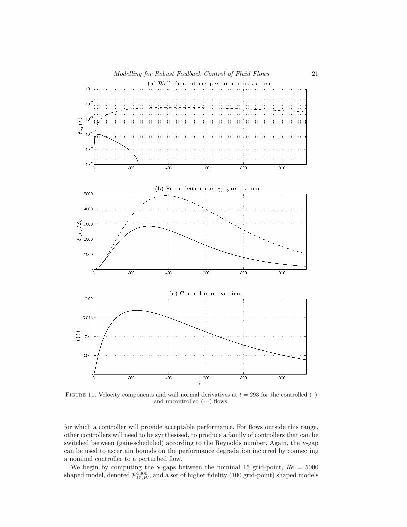
Modelling for Robust Feedback Control of Fluid Flows 21
Figure 11. Velocity components and wall normal derivatives at t = 293 for the controlled (–)and uncontrolled (- -) flows.
for which a controller will provide acceptable performance. For flows outside this range,other controllers will need to be synthesised, to produce a family of controllers that can beswitched between (gain-scheduled) according to the Reynolds number. Again, the ν-gapcan be used to ascertain bounds on the performance degradation incurred by connectinga nominal controller to a perturbed flow.
We begin by computing the ν-gaps between the nominal 15 grid-point, Re = 5000shaped model, denoted P5000
15,W , and a set of higher fidelity (100 grid-point) shaped models

22 B. Ll. Jones, P. H. Heins, E. C. Kerrigan, J. F. Morrison and A. S. Sharma
Figure 12. Evolution of the optimal initial condition in channel flow under the action of theH∞loop-shaping controller. The controller is designed to attenuate the magnitude of streamwiseperturbation wall shear-stresses. Filled contours represent streamwise perturbation velocitieswhilst vectors depict the wall-normal and spanwise velocity perturbation fields. Perturbationenergy gain E(t)/E0 is also shown. Re = 5000, α = 0, β = 2.044. Notice the appearance of thebuffer vortices close to the walls for t > 0.
at Reynolds numbers in the range 500 6 Re 6 50, 000, denotedPRe100,W
. A plot
of δν
(P500015,W ,PRe
100,W
)is shown in Figure 14. As expected, the ν-gaps are smallest for
perturbed flows with Reynolds numbers close to that of the nominal flow and graduallyincrease as the Reynolds number of the perturbed flows departs from the nominal value.Such information can be used, in conjunction with the controller’s stability margin to

Modelling for Robust Feedback Control of Fluid Flows 23
Figure 13. Streamwise vorticity ζx at t = 293 for controlled (–) and uncontrolled (- -) flows.
Figure 14. Variation of the ν-gap metric between nominal and perturbed flows. The nominalsystem is a 15 grid-point model based on Re = 5000, α = 0, β = 2.044. Perturbed models arebased on 100 grid points and Reynolds numbers in the range 500 6 Re 6 50, 000.

24 B. Ll. Jones, P. H. Heins, E. C. Kerrigan, J. F. Morrison and A. S. Sharma
Figure 15. Streamwise wall-shear stress perturbations against time for the uncontrolled (- -)and controlled (–) systems. Here, the controller based on P5000
15,W is applied to a perturbed system
of higher fidelity and higher Reynolds number, P20,000100,W .
determine the range of Reynolds numbers over which the nominal controller can beexpected to perform well. For example, the robust stability margin of the loop-shapingcontroller from Section 3.1 was computed as bopt(P5000
15,W) = 0.68. Provided this exceedsthe ν-gap between the nominal and perturbed flows by a reasonable margin (typicallytaken to be 0.3 - see Appendix A for further details) then one can expect reasonableperformance from the controller. The performance requirement is thus bopt(P5000
15,W) −δν
(P500015,W ,PRe
100,W
)> 0.3 and, referring to Figure 14, this is satisfied for flows in the
range 500 / Re / 20, 000. One would therefore expect the nominal controller to workwell upon Re = 20, 000 flows, and this is confirmed in Figure 15, which shows effectiveattenuation of the streamwise wall-shear stress perturbations for a linearised flow at thisReynolds number.
3.4. DNS results
The results from the previous section were based on a linear model of the flow, andhence neglected the nonlinearity of the Navier-Stokes equations. In this section, the H∞loop-shaping controller is tested upon a nonlinear simulation of a channel flow. Non-linear simulations were performed using a modified version of Channelflow, a spectralDNS code for analysis of incompressible Navier-Stokes flow in channel geometries writ-ten by Gibson (2012). Velocity and pressure are represented as Fourier expansions inthe periodic streamwise and spanwise directions and as Chebyshev polynomials in thewall-normal direction. Channelflow uses the influence-matrix method of Kleiser & Schu-mann (1980) to integrate the Navier-Stokes equations forward in time. This methodsolves the Navier-Stokes equations at each time step via solutions of a sequence of one-dimensional scalar Helmholtz equations for u, v, w and p for each wavenumber pair, with
Modelling for Robust Feedback Control of Fluid Flows 25
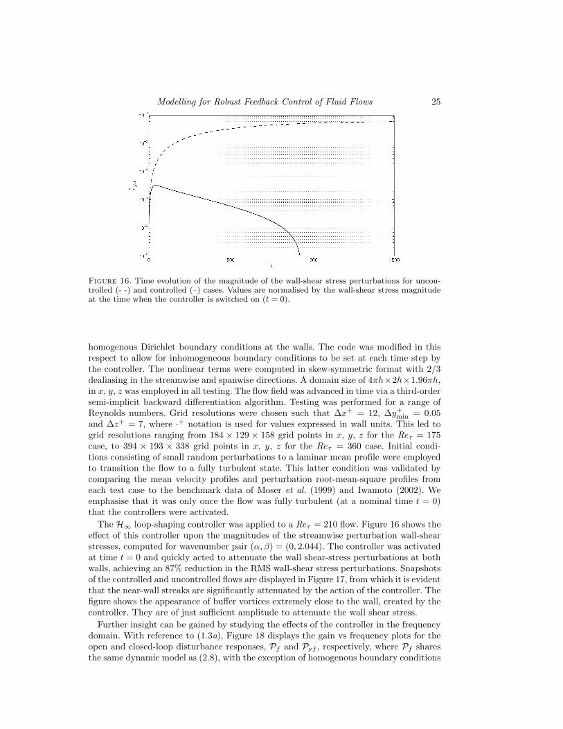
Figure 16. Time evolution of the magnitude of the wall-shear stress perturbations for uncon-trolled (- -) and controlled (–) cases. Values are normalised by the wall-shear stress magnitudeat the time when the controller is switched on (t = 0).
homogenous Dirichlet boundary conditions at the walls. The code was modified in thisrespect to allow for inhomogeneous boundary conditions to be set at each time step bythe controller. The nonlinear terms were computed in skew-symmetric format with 2/3dealiasing in the streamwise and spanwise directions. A domain size of 4πh×2h×1.96πh,in x, y, z was employed in all testing. The flow field was advanced in time via a third-ordersemi-implicit backward differentiation algorithm. Testing was performed for a range ofReynolds numbers. Grid resolutions were chosen such that ∆x+ = 12, ∆y+min = 0.05and ∆z+ = 7, where ·+ notation is used for values expressed in wall units. This led togrid resolutions ranging from 184 × 129 × 158 grid points in x, y, z for the Reτ = 175case, to 394 × 193 × 338 grid points in x, y, z for the Reτ = 360 case. Initial condi-tions consisting of small random perturbations to a laminar mean profile were employedto transition the flow to a fully turbulent state. This latter condition was validated bycomparing the mean velocity profiles and perturbation root-mean-square profiles fromeach test case to the benchmark data of Moser et al. (1999) and Iwamoto (2002). Weemphasise that it was only once the flow was fully turbulent (at a nominal time t = 0)that the controllers were activated.
The H∞ loop-shaping controller was applied to a Reτ = 210 flow. Figure 16 shows theeffect of this controller upon the magnitudes of the streamwise perturbation wall-shearstresses, computed for wavenumber pair (α, β) = (0, 2.044). The controller was activatedat time t = 0 and quickly acted to attenuate the wall shear-stress perturbations at bothwalls, achieving an 87% reduction in the RMS wall-shear stress perturbations. Snapshotsof the controlled and uncontrolled flows are displayed in Figure 17, from which it is evidentthat the near-wall streaks are significantly attenuated by the action of the controller. Thefigure shows the appearance of buffer vortices extremely close to the wall, created by thecontroller. They are of just sufficient amplitude to attenuate the wall shear stress.
Further insight can be gained by studying the effects of the controller in the frequencydomain. With reference to (1.3a), Figure 18 displays the gain vs frequency plots for theopen and closed-loop disturbance responses, Pf and Pyf , respectively, where Pf sharesthe same dynamic model as (2.8), with the exception of homogenous boundary conditions

26 B. Ll. Jones, P. H. Heins, E. C. Kerrigan, J. F. Morrison and A. S. Sharma
Figure 17. Representative snapshot of the controlled (top) and uncontrolled (bottom) flowsat the lower wall, taken at t = 1000. The figure shows contours of perturbation streamwisevelocity (shaded regions) and perturbation streamwise vorticity (solid and dashed lines) in wallunits. The near-wall streaks are significantly attenuated by the controller. The near-wall buffervortices induce just enough streak formation of reverse sign to reduce the wall shear stress.
Modelling for Robust Feedback Control of Fluid Flows 27
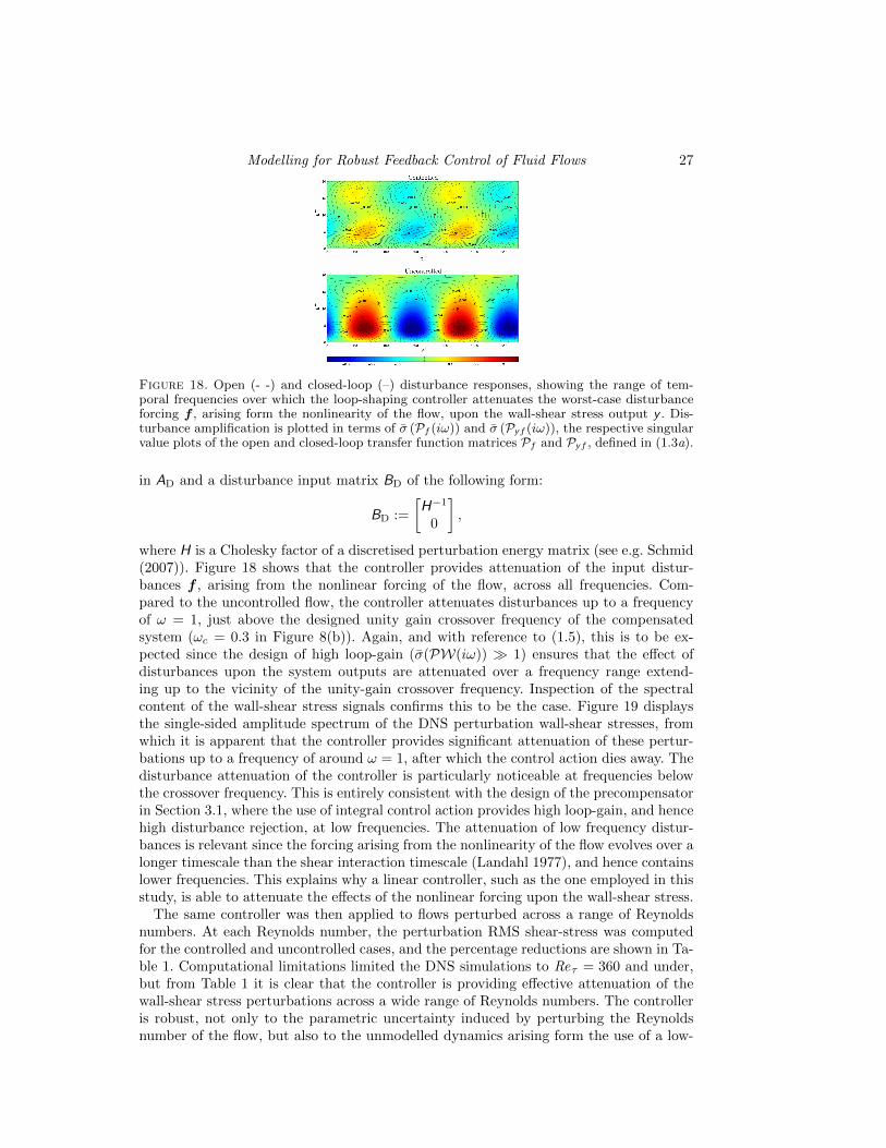
Figure 18. Open (- -) and closed-loop (–) disturbance responses, showing the range of tem-poral frequencies over which the loop-shaping controller attenuates the worst-case disturbanceforcing f , arising form the nonlinearity of the flow, upon the wall-shear stress output y . Dis-turbance amplification is plotted in terms of σ (Pf (iω)) and σ (Pyf (iω)), the respective singularvalue plots of the open and closed-loop transfer function matrices Pf and Pyf , defined in (1.3a).
in AD and a disturbance input matrix BD of the following form:
BD :=
[H−1
0
],
where H is a Cholesky factor of a discretised perturbation energy matrix (see e.g. Schmid(2007)). Figure 18 shows that the controller provides attenuation of the input distur-bances f , arising from the nonlinear forcing of the flow, across all frequencies. Com-pared to the uncontrolled flow, the controller attenuates disturbances up to a frequencyof ω = 1, just above the designed unity gain crossover frequency of the compensatedsystem (ωc = 0.3 in Figure 8(b)). Again, and with reference to (1.5), this is to be ex-pected since the design of high loop-gain (σ(PW(iω)) 1) ensures that the effect ofdisturbances upon the system outputs are attenuated over a frequency range extend-ing up to the vicinity of the unity-gain crossover frequency. Inspection of the spectralcontent of the wall-shear stress signals confirms this to be the case. Figure 19 displaysthe single-sided amplitude spectrum of the DNS perturbation wall-shear stresses, fromwhich it is apparent that the controller provides significant attenuation of these pertur-bations up to a frequency of around ω = 1, after which the control action dies away. Thedisturbance attenuation of the controller is particularly noticeable at frequencies belowthe crossover frequency. This is entirely consistent with the design of the precompensatorin Section 3.1, where the use of integral control action provides high loop-gain, and hencehigh disturbance rejection, at low frequencies. The attenuation of low frequency distur-bances is relevant since the forcing arising from the nonlinearity of the flow evolves over alonger timescale than the shear interaction timescale (Landahl 1977), and hence containslower frequencies. This explains why a linear controller, such as the one employed in thisstudy, is able to attenuate the effects of the nonlinear forcing upon the wall-shear stress.
The same controller was then applied to flows perturbed across a range of Reynoldsnumbers. At each Reynolds number, the perturbation RMS shear-stress was computedfor the controlled and uncontrolled cases, and the percentage reductions are shown in Ta-ble 1. Computational limitations limited the DNS simulations to Reτ = 360 and under,but from Table 1 it is clear that the controller is providing effective attenuation of thewall-shear stress perturbations across a wide range of Reynolds numbers. The controlleris robust, not only to the parametric uncertainty induced by perturbing the Reynoldsnumber of the flow, but also to the unmodelled dynamics arising form the use of a low-

28 B. Ll. Jones, P. H. Heins, E. C. Kerrigan, J. F. Morrison and A. S. Sharma
Figure 19. Single-sided amplitude spectrum of the streamwise wall-shear stress perturbationsfor Reτ = 210. The magnitudes of the wall-shear stress perturbations are significantly lower forthe controlled case (–) at frequencies below the loop crossover frequency (ω = 0.3), compared tothe uncontrolled flow (- -). This is consistent with the linear system responses shown in Figure 18.
Reτ = 175 Reτ = 210 Reτ = 247 Reτ = 281 Reτ = 315 Reτ = 360
87.9% 89.3% 87.5% 87.0% 88.1% 87.9%
Table 1. Percentage RMS reductions in perturbation wall-shear stresses under the control ofthe H∞ loop-shaping controller synthesised from the nominal flow model P5000
15,W .
order spatially discretised model. This is to be expected following on from the resultsof the ν-gap analysis in Figure 14. In addition, the controller demonstrates robustnessto the dynamic uncertainty arising from the nonlinearity of the flow, providing effectiveregulation of the wall-shear stress despite a turbulent initial condition in which the flowis significantly perturbed away from the laminar state assumed in the control model.
4. Conclusions
We have addressed the problem of obtaining models of systems based on the Navier-Stokes equations that provide a priori robust stability and performance bounds for closed-loop flow control. It is suggested that, from the point of view of employing existing linearcontrol systems theory, there are essentially three problems to be tackled: linearisation,spatial discretisation and conversion from a system of DAEs to one of ODEs. We havepresented results that add further evidence to suggest that linear control is effective in thecontrol of wall turbulence even though turbulence is intrinsically nonlinear. Reasons forthis are encapsulated in theories such as RDT, Landahl’s ideas on sheared turbulence orgain-based analyses of turbulence formation. Specifically, by modelling the forcing arisingfrom the nonlinearity of the flow as a disturbance input to the linear flow dynamics, weshowed how the effects of such forcing could be heavily attenuated by designing a feedbackcontroller with high loop-gain over a certain frequency range, and justified this range interms of the timescale separation between linear and nonlinear mechanisms.
The present paper applied two methods for addressing the further issues of discretisa-tion and conversion of equations from physical to state space. For the first, the model-

Modelling for Robust Feedback Control of Fluid Flows 29
refinement procedure was applied to efficiently obtain spatially discretised models of lowstate dimension, from which robust controllers could be readily synthesised, with guaran-teed performance bounds when applied to the actual flow. This is the first instance of thistechnique being applied to a flow control problem. Model refinement is the conceptualopposite of model-reduction based methods, since the starting point of the former ap-proach lay with models of low, rather than high order, and where the emphasis lay uponobtaining models suitable for closed-loop, as opposed to open-loop control. This newapproach to flow control employed established tools from robust control theory, such asthe ν-gap metric and the robust stability margin. In addition, it was argued that coprimefactor uncertainty represents an appropriate choice of uncertainty model for capturingthe inevitable discrepancies that exist between an actual fluid-flow system and a simplercontrol model, hence motivating the use of H∞ loop-shaping control, a technique that tothe best of our knowledge has not previously been applied to the problem of controllingwall turbulence. The problem of converting from physical to state space was overcomeusing a numerical approach that eased the prescription of boundary conditions, comparedto traditional velocity vorticity-based methods.
These techniques were demonstrated upon a simplified problem of skin-friction dragreduction where the controller was based on a linearised, low-order model of the flow.A robust controller was synthesised that provided high attenuation of the perturbationstreamwise wall-shear stresses across a wide range of Reynolds numbers, as evidenced byresults from high fidelity linear simulations and nonlinear DNS. Actuation in the form ofwall-based blowing/suction, vwall, was based on sensing in τyx such that perturbationsof τyx for a given wavenumber pair were minimised. In doing so, the control exerted aninfluence over τyz by setting up near-wall ‘buffer’ vortices.
Future research should address the problem of optimal actuator and sensor placement.Importantly, the framework of gap-metrics and H∞ loop-shaping can be extended toaddress this very issue, as demonstrated by Reinschke & Smith (2003). Loop shapingdesign is a (temporal) frequency domain approach to control systems design. However,it should be noted that frequency does not unambiguously distinguish large structuremoving quickly from small structure moving slowly, and it is the former that makesthe greater contribution to skin friction. In the present work, we have assumed, forsimplicity, that the walls are densely populated with sensors. As a result, the linearisedsystem is rendered observable. Similarly, if in the control objective, small structure playsan important part in generating skin-friction drag then the techniques described in thispaper ensures mesh refinement to an appropriate level by increasing the spatial fidelityof the model. Hence, the model refinement process indicates the appropriate degree ofrefinement required to meet the control objective. For more realistic configurations, futureresearch should also address the consequences of non-conservative domains, i.e. thosein which the nonlinearity of the disturbance field may be taken to be significant, andthe extent to which it may be accommodated by the disturbance rejection framework.For flows exhibiting a more broadband forcing, such as in a turbulent mixing layer forexample, our approach would require a high bandwidth controller to reject high frequencydisturbances, which would likely necessitate the use of fast actuation, which may or maynot be possible. The leads onto the final point that despite the potential effectiveness ofthe linear controllers developed in this paper, it is possible that some form of nonlinearcontrol may provide enhanced performance by selectively exploiting the nonlinearity ofthe flow in some desirable fashion, and designing such controllers could be an interestingavenue of future research.
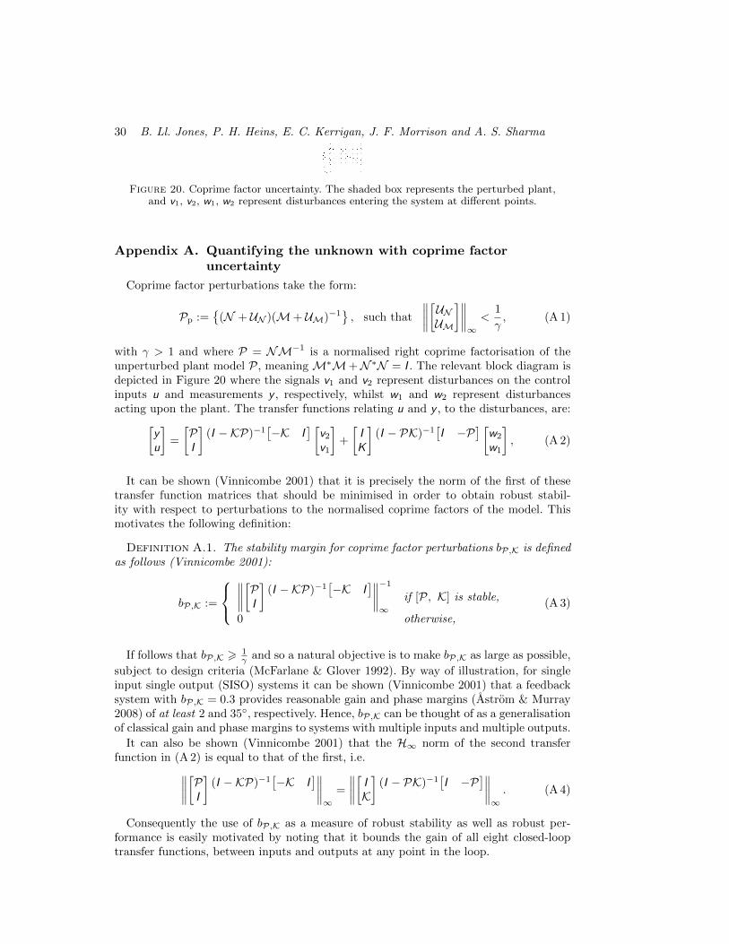
30 B. Ll. Jones, P. H. Heins, E. C. Kerrigan, J. F. Morrison and A. S. Sharma
Figure 20. Coprime factor uncertainty. The shaded box represents the perturbed plant,and v1, v2, w1, w2 represent disturbances entering the system at different points.
Appendix A. Quantifying the unknown with coprime factoruncertainty
Coprime factor perturbations take the form:
Pp :=
(N + UN )(M+ UM)−1, such that
∥∥∥∥[UNUM]∥∥∥∥∞<
1
γ, (A 1)
with γ > 1 and where P = NM−1 is a normalised right coprime factorisation of theunperturbed plant model P, meaningM∗M+N ∗N = I . The relevant block diagram isdepicted in Figure 20 where the signals v1 and v2 represent disturbances on the controlinputs u and measurements y , respectively, whilst w1 and w2 represent disturbancesacting upon the plant. The transfer functions relating u and y , to the disturbances, are:[
yu
]=
[PI
](I −KP)−1
[−K I
] [v2v1
]+
[IK
](I − PK)−1
[I −P
] [w2
w1
], (A 2)
It can be shown (Vinnicombe 2001) that it is precisely the norm of the first of thesetransfer function matrices that should be minimised in order to obtain robust stabil-ity with respect to perturbations to the normalised coprime factors of the model. Thismotivates the following definition:
Definition A.1. The stability margin for coprime factor perturbations bP,K is definedas follows (Vinnicombe 2001):
bP,K :=
∥∥∥∥[PI
](I −KP)−1
[−K I
]∥∥∥∥−1∞
if [P, K] is stable,
0 otherwise,
(A 3)
If follows that bP,K > 1γ and so a natural objective is to make bP,K as large as possible,
subject to design criteria (McFarlane & Glover 1992). By way of illustration, for singleinput single output (SISO) systems it can be shown (Vinnicombe 2001) that a feedbacksystem with bP,K = 0.3 provides reasonable gain and phase margins (Astrom & Murray2008) of at least 2 and 35, respectively. Hence, bP,K can be thought of as a generalisationof classical gain and phase margins to systems with multiple inputs and multiple outputs.
It can also be shown (Vinnicombe 2001) that the H∞ norm of the second transferfunction in (A 2) is equal to that of the first, i.e.∥∥∥∥[PI
](I −KP)−1
[−K I
]∥∥∥∥∞
=
∥∥∥∥[ IK]
(I − PK)−1[I −P
]∥∥∥∥∞. (A 4)
Consequently the use of bP,K as a measure of robust stability as well as robust per-formance is easily motivated by noting that it bounds the gain of all eight closed-looptransfer functions, between inputs and outputs at any point in the loop.

Modelling for Robust Feedback Control of Fluid Flows 31
Appendix B. Computing a standard state-space system fromdescriptor form
Let ED, AD ∈ CnD×nD . The pair (ED,AD) is said to be regular if there exists an s ∈ Csuch that det(sED − AD) 6= 0 (Dai 1989). If (ED,AD) in (2.2a) is regular, there existnonsingular matrices T ,S ∈ Cr×r such that the transformation:
TEDSS−1xD(t) = TADSS
−1xD(t) + TBDu(t), (B 1a)
yields the following system in standard form Gerdin (2006, Lem. 2.3):[I 00 N
] [x(t)χ(t)
]=
[A 00 I
] [x(t)χ(t)
]+
[BG
]u(t), (B 1b)
where N ∈ C(nD−n)×(nD−n) is nilpotent (meaning that Ninp = 0 for some inp ∈ N), Aand B are as in (1.2), G ∈ C(nD−n)×m, I are identity matrices of compatible dimensions
and[x(t)χ(t)
]= S−1xD(t). The matrices in (B 1) are computed as follows (Gerdin 2006;
Schon et al. 2003; Shahzad et al. 2011):(i) Compute the generalised Schur form of the matrix pencil λED − AD so that:
T1(λED − AD)S1 = λ[E1 E2
0 E3
]+[A1 A2
0 A3
], (B 2)
where T1 and S1 are unitary matrices i.e. T ∗1T1 = T1T∗1 = I , and are not to be confused
with T and S in (B 1a). The generalised eigenvalues should be sorted so that the diagonalelements of E1 contain only non-zero elements. The generalised Schur form and thesubsequent reordering can be computed using a QZ algorithm (Golub & Van Loan 1996).
(ii) Solve the following coupled Sylvester equation to obtain the matrices L and R:
E1R + LE3 = −E2, (B 3a)
A1R + LA3 = −A2. (B 3b)
The solution to (B 3) can be obtained by solving for L in:
A1E−11 LE3A
−13 − L−
(A2 − A1E
−11 E2
)A−13 = 0, (B 4a)
and substituting to obtain R:
R = −E−11 E2 − E−11 LE3. (B 4b)
(iii) Form the matrices in (B 1) as follows:
T =
[E−11 0
0 A−13
] [I L0 I
]T1, S = S1
[I R0 I
], (B 5a)
A = E−11 A1,
[BG
]= TBD, N = A−13 E3. (B 5b)
(iv) Provided (Gerdin 2006) NjG = 0 for all j ∈ N > 1, then (2.2b) is given by:
y(t) = CDS
[x(t)χ(t)
]=[C J
] [x(t)χ(t)
]= Cx(t) + Du(t). (B 6)
where J ∈ Cq×(nD−n) and D := −JG . This completes the numerical conversion of adescriptor state-space system (2.2) into a standard state-space system (1.2).
REFERENCES

32 B. Ll. Jones, P. H. Heins, E. C. Kerrigan, J. F. Morrison and A. S. Sharma
Aamo, O. M. & Krstic, M. 2003 Flow control by feedback: Stabilization and Mixing . Springer.
Antoulas, A. C. 2005 An overview of approximation methods for large scale dynamical sys-tems. Annual reviews in Control 29, 181–190.
Arthur, G. G., McKeon, B. J., Dearing, S. S., Morrison, J. F. & Cui, Z. 2006 Man-ufacture of micro-sensors and actuators for flow control. Microelectronic Engineering 83,1205–1208.
Balas, M. J. 1978 Feedback control of flexible systems. IEEE Transactions on AutomaticControl 23, 673–679.
Baramov, L., Tutty, O. R. & Rogers, E. 2004 H∞ Control of Nonperiodic Two-DimensionalChannel Flow. IEEE Transactions on Control Systems Technology 12 (111-122).
Batchelor, G. K. & Townsend, A. A. 1956 Turbulent diffusion. In Surveys in Mechanics(ed. G. K. Batchelor & R. M. Davies), pp. 352–399. Cambridge University Press.
Bewley, T. R. 2001 Flow control: new challenges for a new renaissance. Progress in AerospaceSciences 37, 21–58.
Bewley, T. R. & Liu, S. 1998 Optimal and robust control and estimation of linear paths totransition. Journal of Fluid Mechanics 365, 305–349.
Bobba, K. M. 2004 Robust flow stability: Theory, computations and experiments in near wallturbulence. PhD thesis, California Institute of Technology, Pasadena, California, USA.
Boyd, J. P. 2001 Chebyshev and Fourier Spectral Methods, 2nd edn. Dover, Mineola, New York.
Bradshaw, P. 1967 ‘Inactive’ motion and pressure fluctuations in turbulent boundary layers.Journal of Fluid Mechanics 30, 241–258.
Bushnell, D. M. 2003 Aircraft drag reduction - a review. Journal of Aerospace Engineering217, 1–18.
Butler, K. M. & Farrell, B. F. 1992 Three-dimensional optimal perturbations in viscousshear flow. Phys. Fluids A 4 (8), 1637–1650.
Chernyshenko, S. I. & Baig, M. F. 2005 The mechanism of streak formation in near-wallturbulence. Journal of Fluid Mechanics 544, 99–131.
Cherubini, S., De Palma, P., Robinet, J.-Ch. & Bottaro, A. 2010 Rapid path to transitionvia nonlinear localized optimal perturbations in a boundary-layer flow. Physical Review E82 (6), 066302.
Cherubini, S., De Palma, P., Robinet, J.-Ch. & Bottaro, A. 2011 The minimal seed ofturbulent transition in the boundary layer. Journal of Fluid Mechanics 689, 221–253.
Choi, H., Moin, P. & Kim, J. 1993 Direct numerical simulation of turbulent flow over riblets.Journal of Fluid Mechanics 255, 503–539.
Chu, Y., Glover, K. & Dowling, A. P. 2003 Control of combustion oscillations via H∞loop-shaping, µ-analysis and Integral Quadratic Constraints. Automatica 39, 219–231.
Collis, S. S., Joslin, R. D., Seifert, A. & Theofilis, V. 2004 Issues in active flow control:theory, control, simulation and experiment. Progress in Aerospace Sciences 40, 237–289.
Corbett, J. J. & Koehler, H. W. 2003 Updated emissions from ocean shipping. Journal ofGeophysical Research 108(D20), 4650–4664.
Couchman, I. J. & Kerrigan, E. C. 2010 Control of mixing in a Stokes’ fluid flow. Journalof Process Control 20, 1103–1115.
Curtain, R. & Morris, K. 2009 Transfer functions of distributed parameter systems: A tuto-rial. Automatica 45, 1101–1116.
Dahan, J. A., Morgans, A. S. & Lardeau, S. 2012 Feedback control for form-drag reductionon a bluff body with a blunt trailing edge. J. Fluid Mech. 704, 360–387.
Dai, L. 1989 Singular Control Systems. Springer-Verlag.
Dullerud, G. & Paganini, F. 2000 A Course in Robust Control Theory: A Convex Approach.Springer.
Dunn, D. C. & Morrison, J. F. 2003 Anisotropy and energy flux in wall turbulence. J. FluidMech. 491, 353–378.
Farrell, B. & Ioannou, J. 1993 Stochastic forcing of the linearized Navier-Stokes equations.Phys. Fluids 5 (11), 2600–2609.
Farrell, B. & Ioannou, J. 1996 Turbulence suppression by active control. Phys. Fluids 8 (5),1257–1268.
Ferziger, J. H. & Peric, M. 1997 Computational Methods for Fluid Dynamics. Springer.
Modelling for Robust Feedback Control of Fluid Flows 33
Fish, F. E. & Lauder, G. V. 2006 Passive and Active Flow Control by Swimming Fishes andMammals. Annual Review of Fluid Mechanics 38, 193–224.
Frederick, M., Kerrigan, E. C. & Graham, J. M. R. 2010 Gust alleviation using rapidlydeployed trailing-edge flaps. Journal of Wind Engineering and Industrial Aerodynamics98 (12), 712–723.
Gad-el-Hak, M. 2000 Flow control: Passive, Active and Reactive Flow Management . Cam-bridge University Press.
Gallas, Q., Carroll, B., Cattafesta, L., Holman, R., Nishida, T. & Sheplak, M. 2003Lumped Element Modeling of Piezoelectric-Driven Synthetic Jet Actuators. AIAA Journal41, 240–247.
Gerdin, M. 2006 Identification and Estimation for Models Described by Differential-AlgebraicEquations. PhD thesis, Linkoping University, Sweden.
Gibson, J. F. 2012 Channelflow: A spectral Navier-Stokes simulator in C++. Tech. Rep.. U.New Hampshire.
Glad, T. & Ljung, L. 2000 Control Theory: Multivariable and Nonlinear Methods. Taylor &Francis.
Golub, G. H. & Van Loan, C. F. 1996 Matrix Computations, 3rd edn. The Johns HopkinsUniversity Press.
Hamilton, J. M., Kim, J. & Waleffe, F. 2006 Regeneration mechanisms of near-wall turbu-lence structures. Journal of Fluid Mechanics 287, 317–348.
Hanson, R., Lavoie, P., Naguib, A. M. & Morrison, J. F. 2010 Transient growth instabilitycancelation by a plasma actuator array. Experiments in Fluids 49 (6), 1339.
Hoepffner, J., Chevalier, M., Bewley, T. R. & Henningson, D. S. 2005 State estimationin wall-bounded flow systems. Part 1. Perturbed laminar flows. Journal of Fluid Mechanics534, 263–294.
Hogberg, M., Bewley, T. R. & Henningson, D. S. 2003 Linear feedback control and esti-mation of transition in plane channel flow. J. Fluid Mech. 481, 149–175.
Holmes, P., Lumley, J. L. & Berkooz, G. 1996 Turbulence, Coherent Structures, DynamicalSystems and Symmetry . Cambridge, UK: Cambridge University Press.
Hunt, J. C. R. & Carruthers, D. J. 1990 Rapid distortion theory and some of the ‘problems’of turbulence. J. Fluid Mech. 212, 497–532.
Hyde, R. A., Glover, K. & Shanks, G. T. 1995 VSTOL first flight of an H-infinty controllaw. Computing and Control Engineering Journal 6 (1), 11–16.
Iwamoto, K. 2002 Database of fully developed channel flow. Tech. Rep. ILR-0201. Departmentof Mechanical Engineering, The University of Tokyo.
Jones, B. L. & Kerrigan, E. C. 2010 When is the discretization of a spatially distributedsystem good enough for control? Automatica 46 (9), 1462–1468.
Jones, B. Ll., Kerrigan, E. C., Morrison, J. F. & Zaki, T. A. 2011 Flow Estimationof Boundary Layers Using DNS Based Wall Shear Information. International Journal ofControl 84, 1310–1325.
Jovanovic, M. R. & Bamieh, B. 2005 Componentwise energy amplification in channel flows.J. Fluid Mech. 534, 145–183.
Kim, J. 1989 On the structure of pressure fluctuations in simulated turbulent channel flow. J.Fluid Mech. 205, 421–451.
Kim, J. 2003 Control of turbulent boundary layers. Phys. Fluids 15 (5).
Kim, J. & Bewley, T. R. 2007 A linear systems approach to flow control. Annual Review ofFluid Mechanics 39, 383–417.
Kim, J. & Lim, J. 2000 A linear process in wall-bounded turbulent shear flows. Phys. Fluids12 (8).
Kleiser, L. & Schumann, U. 1980 Treatment of incompressibility and boundary conditionsin 3-d numerical spectral simulations of plane channel flows. In Conference on NumericalMethods in Fluid Mechanics, 3rd, Cologne, West Germany, October 10-12, 1979, Proceed-ings. (A80-38252 15-34) Braunschweig, Friedr. Vieweg und Sohn Verlagsgesellschaft mbH ,pp. 165–173.
Landahl, M. T. 1967 A wave guide model for turbulent shear flow. J. Fluid Mech. 29, 441–459.
Landahl, M. T. 1975 Wave Breakdown and Turbulence. SIAM J. Appl. Math. 28 (4), 735–756.

34 B. Ll. Jones, P. H. Heins, E. C. Kerrigan, J. F. Morrison and A. S. Sharma
Landahl, M. T. 1977 Dynamics of boundary layer turbulence and the mechanism of dragreduction. Phys. Fluids 20 (10), S55–S63.
Lee, K. H., Cortelezzi, L., Kim, J. & Speyer, J. 2001 Application of reduced-order controllerto turbulent flows for drag reduction. Physics of Fluids 13 (5), 1321–1330.
Lee, M. J., Kim, J. & Moin, P. 1990 Structure of turbulence at high shear rate. J. Fluid Mech.216, 561–583.
Lim, J. 2003 Control of wall-bounded turbulent shear flows using modern control theory. PhDthesis, University of California, Los Angeles.
Lu, Q., Bowyer, R. & Jones, B. Ll. 2014 Analysis and design of Coleman transform-based individual pitch controllers for wind-turbine load reduction. Wind Energy (Doi:10.1002/we.1769).
Luaga, E. & Bewley, T. R. 2004 Performance of a linear robust control strategy on a nonlinearmodel of spatially developing flows. Journal of Fluid Mechanics 512, 343–374.
McFarlane, D. & Glover, K. 1992 A loop shaping design procedure using H∞ synthesis.IEEE Transactions on Automatic Control 37 (6), 759–769.
McKeon, B. J. & Sharma, A. S. 2010 A critical-layer framework for turbulent pipe flow.Journal of Fluid Mechanics 658, 336–382.
McKeon, B. J., Sharma, A. S. & Jacobi, I. 2013 Experimental manipulation of wall turbu-lence - a systems approach. Physics of Fluids 25 (3), 031301.
McKernan, J. 2006 Control of plane Poiseuille flow: A theoretical and computational investi-gation. PhD thesis, Cranfield University.
McKernan, J., Papadakis, G. & Whidborne, J. F. 2006 Linear state-space representationof plane poiseuille flow for control design - a tutorial. Int. J. Modelling, Identification andControl 1 (4), 272–280.
Morrison, J. F. 2007 The interaction between inner and outer regions of turbulent wall-bounded flow. Phil. Trans. R. Soc. A 365 (1852), 683–698.
Moser, R., Kim, J. & Mansour, N. N. 1999 Direct numerical simulation of turbulent channelflow up to Reτ = 590. Phys. Fluids 11 (4), 943–945.
Pringle, C. C. T. & Kerswell, R. R. 2010 Using nonlinear transient growth to constructthe minimal seed for shear flow turbulence. Physical review letters 105 (15), 154502.
Pringle, C. C. T., Willis, A. P. & Kerswell, R. R. 2012 Minimal seeds for shear flowturbulence: using nonlinear transient growth to touch the edge of chaos. Journal of FluidMechanics 702, 415–443.
Astrom, K. J. & Murray, R. M. 2008 Feedback Systems: An Introduction for Scientists andEngineers. Princeton University Press.
Reinschke, J. & Smith, M. C. 2003 Designing robustly stabilising controllers for LTI spatiallydistributed systems using coprime factor synthesis. Automatica 39, 193–203.
Robinson, S. K. 1991 Coherent motions in the turbulent boundary layer. Annual Review ofFluid Mechanics 23, 601.
Rowley, C. W. 2005 Model reduction for fluids, using balanced proper orthogonal decomposi-tion. International Journal of Bifurcation and Chaos 15 (3), 997–1013.
Schmid, P. J. 2007 Nonmodal stability theory. Annual Review of Fluid Mechanics 39, 129–162.Schmid, P. J. & Henningson, D. S. 2000 Stability and Transition in Shear Flows. Springer.Schon, T., Gerdin, M., Glad, T. & Gustaffson, F. 2003 A modeling and filtering framework
for linear implicit systems. In Proceedings of the 42nd IEEE Conference on Decision andControl , pp. 892–897. Maui, Hawaii, USA.
Semeraro, O., Bagheri, S., Brandt, L. & Henningson, D. S. 2011 Feedback control ofthree-dimensional optimal disturbances using reduced-order models. Journal of Fluid Me-chanics 677, 63–102.
Shahzad, A., Jones, B. L., Kerrigan, E. C. & Constantinides, G. A. 2011 An efficientalgorithm for the solution of a coupled Sylvester equation appearing in descriptor systems.Automatica 47, 244–248.
Sharma, A. S. & McKeon, B. J. 2013 On coherent structure in wall turbulence. Journal ofFluid Mechanics 728, 196–238.
Sharma, A. S., Morrison, J. F., McKeon, B. J., Limebeer, D. J. N., Koberg, W. H. &Sherwin, S. J. 2011 Relaminarisation of Reτ = 100 channel flow with globally stabilisinglinear feedback control. Physics of Fluids 23 (12), 125105.

Modelling for Robust Feedback Control of Fluid Flows 35
Skogestad, S. & Postlethwaite, I. 2005 Multivariable Feedback Control . John Wiley & Sons,Ltd.
Sturzebecher, D. & Nitsche, W. 2003 Active cancellation of tollmien-schlichting instabilitieson a wing using multi-channel sensor actuator systems. International Journal of Heat andFluid Flow 24, 572–583.
Townsend, A. A. 1961 Equilibrium layers and wall turbulence. Journal of Fluid Mechanics11, 97–120.
Trefethen, L. N. & Embree, M. 2005 Spectra and Pseudospectra - The Behaviour of Non-normal Matrices and Operators. Princeton University Press.
Trefethen, L. N., Trefethen, A. E., Reddy, S. C. & Driscoll, T. A. 1993 Hydrodynamicstability without eigenvalues. Science 261.
Vinnicombe, G. 2001 Uncertainty and Feedback . Imperial College Press.Weideman, J. A. C. & Reddy, S. C. 2000 A MATLAB differentiation matrix suite. ACM
Transactions on Mathematical Software 26 (4), 465–519.Willcox, K. & Peraire, J. 2002 Balanced model reduction via the proper orthogonal decom-
position. AIAA Journal 40 (11).Zhou, K. & Doyle, J. C. 1998 Essentials of Robust Control . Prentice Hall.Zhou, K., Doyle, J. C. & Glover, K. 1996 Robust and optimal control . Prentice Hall.