brush control feasibility study for the o.h. ivie ... · brush control feasibility study for the...

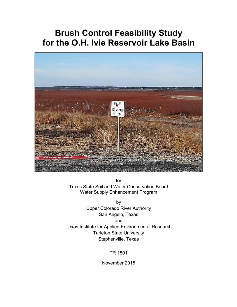
Brush Control Feasibility Study for the O.H. Ivie Reservoir Lake Basin

for Texas State Soil and Water Conservation Board

Water Supply Enhancement Program

by Upper Colorado River Authority

San Angelo, Texas and

Texas Institute for Applied Environmental Research Tarleton State University

Stephenville, Texas

TR 1501

November 2015

O.H. Ivie Reservoir Feasibility Study

ii

Acknowledgements Funding for this project was provided by the Texas State Soil and Water Conservation Board (TSSWCB) through Cooperative Agreement 13007-2013-04 with the Upper Colorado River Authority (UCRA). Under subcontract arrangements with the UCRA, the Texas Institute for Applied Environmental Research (TIAER) at Tarleton State University embarked on the hydrologic simulations required for a feasibility study under the TSSWCB’s Water Supply Enhancement Program (WSEP). The UCRA and TIAER appreciate the support of the TSSWCB in funding and providing direction for this project as well as their review of this report.

The technical assistance to define needed crop growth parameters for saltcedar and willow baccharis as input to SWAT was provided by Dr. James Kiniry, Dr. Mike White and Ms. Amber Williams at the U.S. Department of Agriculture – Agricultural Research Service – Grassland, Soil and Water Research Laboratory (USDA-ARS-GSWRL). Additional technical assistance in defining crop rotations and animal grazing for Runnels County were provided by Mr. Marty Gibbs and Mr. Richard Mizenmayer of Texas A&M AgriLife Extension Service. Dr. Kannan Narayanan and Dr. Ali Saleh at TIAER provided invaluable assistance and guidance on the operation of the SWAT model for this project. The assistance provided by all these individuals is very much appreciated and added to the technical rigor of this study. Further, the timely review comments of Mr. Chuck Brown, Director of Operations at UCRA, were beneficial and greatly appreciated.

Primary Authors: Larry Hauck, Lead Scientist, TIAER Ujwal Pandey, Senior Research Associate, TIAER

Cover photo: Photograph taken January 22, 2014 at Concho Park marina showing low reservoir levels in O.H. Ivie Reservoir and the saltcedar (reddish-orange color) infestation of the dry, exposed reservoir basin.


iii

Table of Contents Introduction ................................................................................................................................... 1

Purpose .................................................................................................................................................... 1

Description of the Project Area ............................................................................................................ 2

Model Development ...................................................................................................................... 6

Description of Soil and Water Assessment Tool ............................................................................... 6

Modeling Approach ................................................................................................................................ 7

Delineation of Modeled Areas .............................................................................................................. 9

Elm Creek SWAT Model Development ........................................................................................... 9

O.H. Ivie Reservoir Basin SWAT Model Development ............................................................... 15

Temporal Model Input ...................................................................................................................... 20

Elm Creek Watershed Model Calibration .................................................................................... 21

Calibration Process .............................................................................................................................. 21

Calibration Results ............................................................................................................................... 23

Model Calibration Discussions ........................................................................................................... 27

Simulation of Effects of Brush Management ............................................................................... 29

Simulation Methods ............................................................................................................................. 29

Standard Brush Control Evaluation Method ................................................................................. 29

Water Yield Results ............................................................................................................................. 30

Summary ..................................................................................................................................... 31

References .................................................................................................................................. 33

Appendix A: Evaluation Method for Additional Water Savings ................................................... 37

List of Figures Figure 1. Photograph of the Concho River arm of O.H. Ivie Reservoir showing low

reservoir levels and heavy brush encroachment into the immediate basin. ................ 2

Figure 2. Watershed of O.H. Reservoir showing upstream reservoirs .......................................... 3

Figure 3. USGS daily data for the period 1998-2014 for O.H. Ivie Reservoir. .............................. 4

Figure 4. Annual rainfall for the O.H. Ivie Reservoir area during the period of 1995-2014 ........ 5

Figure 5. USGS stations near the O.H. Ivie Reservoir ..................................................................... 8

Figure 6. Slope classification of the Elm Creek watershed ........................................................... 10

Figure 7. SWAT subbasin delineation of Elm Creek watershed ................................................... 11


iv

Figure 8. Land cover of Elm Creek watershed ................................................................................ 12 Figure 9. Hydrologic soil groupings for Elm Creek watershed based on SURGO level

data. ....................................................................................................................................... 14

Figure 10. Slope classification for immediate basin of O.H. Ivie Reservoir ................................... 15

Figure 11. Land cover for Water-Level Condition 1 of immediate basin of O.H. Reservoir ........ 17

Figure 12. Land cover for Water-Level Condition 2 of immediate basin of O.H. Reservoir ........ 18 Figure 13. Hydrologic soil groupings for immediate basin of O.H. Ivie Reservoir based on

SURGO level data obtained from county soil survey reports ....................................... 19 Figure 14. Time series of measured and simulated monthly streamflow for Elm Creek

watershed, 1995-2010. ....................................................................................................... 25 Figure 15. Scatter plot of measured and simulated monthly streamflow for Elm Creek

watershed, 1995-2010. ....................................................................................................... 25 Figure 16. Time series of measured and simulated annual streamflow for Elm Creek

watershed, 1995-2010. ....................................................................................................... 26 Figure 17. Scatter plot of measured and simulated annual streamflow for Elm Creek

watershed, 1995-2010. ....................................................................................................... 26

List of Tables Table 1. Slope classification description of Elm Creek watershed .............................................. 10 Table 2. Land cover of Elm Creek watershed by classification categories in the 2006

NLCD ..................................................................................................................................... 13

Table 3. Slope classification description for immediate basin of O.H. Ivie Reservoir .............. 16

Table 4. Land cover for Water-Level Condition 1 of immediate basin of O.H. Reservoir ........ 17

Table 5. Land Cover for Water-Level Condition 2 of immediate basin of O.H. Reservoir ....... 18

Table 6. Process-related parameters adjusted in calibration of SWAT Elm Creek model ...... 24

Table 7. Hydrologic calibration statistics and results of SWAT Elm Creek model .................... 27 Table 8. Predicted increase in water yield from brush control in the immediate basin of

O.H. Ivie Reservoir; annual average for 1995-2010 ...................................................... 31


1

Introduction The Texas Legislature has designated the Texas State Soil and Water Conservation Board (TSSWCB) as the agency responsible for administering the Water Supply Enhancement Program (WSEP). The objective of the WSEP is to increase availability of surface and ground water through selective control of brush species that are detrimental to water conservation (TSSWCB, 2014). The reported potential benefits of brush control include enhanced water yield, conserved water lost to evapotranspiration, recharged groundwater and aquifers, enhanced spring and stream flows, improved soil health, restored native wildlife habitat by improving rangeland, improved livestock grazing distribution, protected water quality and reduced soil erosion, wildfire suppression by reducing hazardous fuels, and management of invasive species (NRCS, 2009; TSSWCB, 2015). Such resources as Jones and Gregory (2008) and Rainwater et al. (2008) provide an overview on the effectiveness of brush control plus the complexities associated with scientifically establishing the increases in water yield from brush control.

The TSSWCB WSEP requires that feasibility studies be performed using computer models to predict water yield changes for watersheds where brush control is being considered. The feasibility studies are reviewed and evaluated to prioritize for the brush control projects that have the best opportunities to increase water yields in areas of water supply needs. TSSWCB (2014) provides detailed guidance for application of the appropriate models for feasibility studies on proposed brush control projects. To provide for consistency and comparability between studies, the WSEP guidance recommends application of the Soil and Water Assessment Tool (SWAT) or Ecological Dynamics Simulation (EDYS) model, though other models will be considered and reviewed by the WSEP Science Advisory Committee.

While both SWAT and EDYS have been successfully applied to predict the potential changes in water yield from brush control, SWAT has been more widely applied than EDYS. Evaluation of water yield enhancement in Gonzales County as performed using EDYS was reported in McLendon et al. (2012). SWAT was the early model of choice for evaluating water yield increases from brush control as encapsulated in USDA and Texas A&M (2002) and Connor et al. (2000) where individual studies are combined into one report providing predicted water yield increases from brush control for eight Texas watersheds. Further, SWAT has continued to be applied in more recent brush control feasibility studies (e.g., Bumgarner and Thompson, 2012).

Purpose The purpose of this report is to document the development, calibration, and application of a SWAT model of the immediate basin of O.H. Ivie Reservoir to predict the effects of brush management on water yields under the TSSWCB WSEP feasibility study guidance. Due to an extended multi-year period of low water levels in O.H. Ivie Reservoir, much of the immediate basin has been exposed allowing extensive, dense infestations of undesirable brush species; most notably saltcedar (Tamarix spp.) and willow baccharis (Baccharis salicna T&G) as well as


2

limited areas of mesquite (Prosopis glandulosa) infestation (see Cover Photograph as well as Figure 1). The SWAT application was used to estimate changes in water yield from the exposed basin under the conditions of the replacement of the invasive brush species with grasslands.

Figure 1. Photograph of the Concho River arm of O.H. Ivie Reservoir showing low reservoir levels and heavy brush encroachment into the immediate basin. Photograph taken from FM 1929 bridge looking north on January 22, 2014; saltcedar appear as reddish orange color and willow baccharis as light greenish-brown.

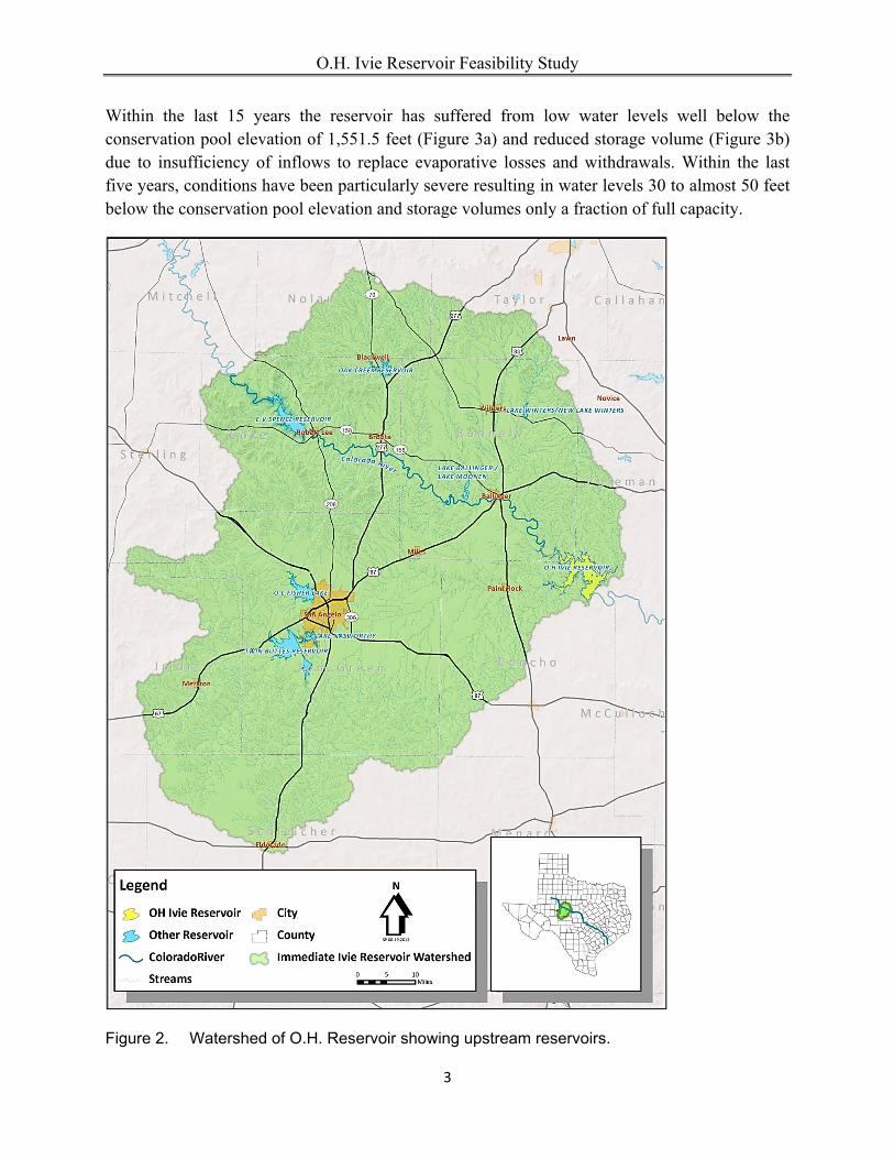
Description of the Project Area The dam to O.H. Ivie Reservoir was completed and storage began March 15, 1990. According to information of the U.S. Geological Survey (USGS) for station 0813660 (O.H. Ivie Reservoir near Voss, TX), the drainage area of the reservoir is 24,038 square miles (sq. mi.) of which it is estimated that 11,391 sq. mi. probably are noncontributing. In addition, E.V. Spence Reservoir on the Colorado River and Twin Buttes Reservoir, Lake Nasworthy, and O.C. Fisher Lake within the Concho River watershed are all positioned upstream of O.H. Ivie Reservoir. Consequentially, these upstream reservoirs reduce the effective drainage area of the O.H. Ivie Reservoir under all but the wettest conditions to about 3,400 sq. mi (Figure 2). At conservation pool elevation, O.H. Ivie Reservoir has a storage capacity of 554,000 acre-feet and a surface area of 19,100 acres. The Colorado River Municipal Water District owns and operates O.H. Ivie Reservoir as well as two other major surface reservoirs and four groundwater well fields for the purpose of supplying municipal water to the cities of Abilene, Big Spring, Midland, Odessa, San Angelo, Snyder and other smaller communities and Millersview-Doole Water Supply Cooperation (CRMWD, 2015).


3

Within the last 15 years the reservoir has suffered from low water levels well below the conservation pool elevation of 1,551.5 feet (Figure 3a) and reduced storage volume (Figure 3b) due to insufficiency of inflows to replace evaporative losses and withdrawals. Within the last five years, conditions have been particularly severe resulting in water levels 30 to almost 50 feet below the conservation pool elevation and storage volumes only a fraction of full capacity.

Figure 2. Watershed of O.H. Reservoir showing upstream reservoirs.


4

Figure 3. USGS daily data for the period 1998-2014 for O.H. Ivie Reservoir. Figure 3a provides water elevations, Figure 3b provides reservoir storage. Source: USGS (2015a)


5

These lowered water levels have resulted in a proliferation of saltcedar and willow baccharis in the immediate basin of the reservoir. Saltcedar and willow baccharis are classified as phreatophytes, which as deep-rooted plants capture a significant portion of their water needs from the phreatic zone (zone of saturation) and the layer of soil just above the phreatic zone. Both species are highly competitive invasive species that replace other more desirable grass, brush, and tree species. Saltcedar is a non-native invasive species whereas willow baccharis is a native species with invasive tendency in moist open areas e.g., exposed lake bed as a result of falling water levels. Because of the density of their stands and deep roots, saltcedar and willow baccharis often consume more water through evapotranspiration than more desirable plants. The detrimental impacts on water supply of phreatophytes are documented in many reports and in the scientific literature of which a sampling is Gregory and Hatler (2008), Hatler and Hart (2009), Homes (1998), and Robinson (1958).

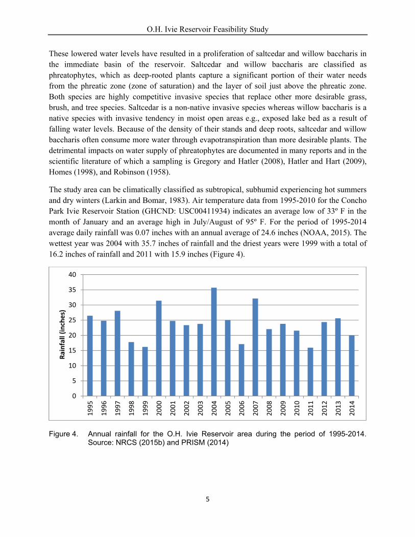
The study area can be climatically classified as subtropical, subhumid experiencing hot summers and dry winters (Larkin and Bomar, 1983). Air temperature data from 1995-2010 for the Concho Park Ivie Reservoir Station (GHCND: USC00411934) indicates an average low of 33º F in the month of January and an average high in July/August of 95º F. For the period of 1995-2014 average daily rainfall was 0.07 inches with an annual average of 24.6 inches (NOAA, 2015). The wettest year was 2004 with 35.7 inches of rainfall and the driest years were 1999 with a total of 16.2 inches of rainfall and 2011 with 15.9 inches (Figure 4).

Figure 4. Annual rainfall for the O.H. Ivie Reservoir area during the period of 1995-2014. Source: NRCS (2015b) and PRISM (2014)

0

5

10

15

20

25

30

35

40

1995

1996

1997

1998

1999

2000

2001

2002

2003

2004

2005

2006

2007

2008

2009

2010

2011

2012

2013

2014

Rainfall (inches)


6

Model Development

Description of Soil and Water Assessment Tool SWAT is a physically-based watershed and landscape simulation model developed by the USDA-Agricultural Research Service (Arnold et al., 1998). Major components of the model include hydrology, weather, erosion, soil, temperature, crop growth, nutrients, pesticides and agricultural management. SWAT also has the ability to predict changes in sediment, nutrients (such as organic and inorganic nitrogen and organic and soluble phosphorus), pesticides, dissolved oxygen, bacteria and algae loadings from different management conditions in large un-gaged basins. SWAT operates on a daily time step and can be used for long-term simulations. The model output is available in daily, monthly and annual time scales.

For modeling purposes, the watershed to be simulated is partitioned into subwatersheds, which in SWAT are referred to as subbasins. Each subbasin is comprised of the land area within its boundaries as well as a stream reach. Collectively the subbasins represent the entire domain of the modeled area and the reaches define the stream drainage network of the watershed. Hydrologic response units (HRUs) provide an additional subdivision representing lumped land areas within each subbasin that are comprised of unique land cover, soil, and management combinations. Within the computations of SWAT, a water balance is performed on each HRU that takes into account precipitation, surface runoff, soil water content, evapotranspiration, lateral subsurface flow, and the amount of water leaving the soil profile. Further, the life cycle of land cover (e.g., crops, forest, rangeland, urban) specified for each HRU is simulated in a process mode. Within the reach of each SWAT subbasin, the surface water is routed including any flow contributions from upstream subbasins, transmission and evaporation losses, and surface and subsurface flow contributions from the HRUs within the subbasin. SWAT is typically operated on a daily time step and can be applied to simulate watershed conditions for multiple years and decades. A complete description of the SWAT model, its features and theoretical development are provided in Neitsch et al. (2011).

For this feasibility study, the water quality simulation capabilities of SWAT were not required regarding nutrients, sediments, and pesticides. Rather the focus was on the hydrologic features of the model. SWAT provides two options for estimating surface runoff: the Soil Conservation Service (SCS) curve-number (CN) runoff equation and the Green and Ampt infiltration method (Neitsch et al., 2011). The SCS runoff equation was selected for this study, because it uses daily precipitation data, whereas the Green and Ampt method requires sub-daily precipitation data, which were not available for the study area. The SCS runoff equation is an empirical model involving rainfall-runoff relationships developed using the CN to provide a consistent basis of estimating amounts of runoff (Neitsch et al., 2011; SCS, 1986). The value of the CN is a function of both the land use and the soil hydrologic group, where a higher value results in the computation of greater runoff than a smaller value.


7

The 2012 version of SWAT was used for this application (Arnold et al., 2013). ArcSWAT 2012.10.0.13 for ArcGIS 10.0 and SWATeditor 2012.10.0.13 were used to delineate the study area into subbasins.

Modeling Approach The WSEP policy for feasibility studies stipulates that the model must be calibrated using graphical and statistical methods to observational streamflow data to establish the reliability of the model in representing the real-world system and for predicting changes in the water yield from brush control scenarios (TSSWCB, 2014). Typically the observational data required for calibration consists of daily flow from one or more USGS streamflow gaging stations located within the study area. In situations, such as for this project, where the study area does not contain a streamflow gaging station, the WSEP policy states:

If the watershed of interest does not contain a USGS gage, data from either the nearest downstream gage or a gage in a neighboring watershed may be used to calibrate the model. The decision to use data from either a downstream gage or a gage in a neighboring watershed should be based on an analysis of the similarities in hydrology and land use to the watershed of interest. (TSSWCB, 2014, p. 3)

Because the project study area consists of the immediate exposed basin of O.H. Ivie Reservoir, there are no streamflow gages located within the area. The policy guidance, therefore, is to use data from a downstream gage or a gage in a neighboring watershed for calibration purposes. Four candidate USGS streamflow gages are located within reasonable proximity of the study area:

1) USGS station 08127000, Elm Creek at Ballinger, Texas, 2) USGS station 08126380, Colorado River near Ballinger, Texas, 3) USGS station 08136500, Concho River at Paint Rock, Texas, and 4) USGS station 08316700, Colorado River near Stacy, Texas.

The location of each station is depicted on Figure 5.

The Colorado River near Ballinger (station 08126380) and the Concho River at Paint Rock (08136500) were not considered reasonable sources of calibration data, because use of the data from either station would necessitate modeling a large watershed (well over 1,000 sq. mi. each) that included areas distant from the study area and contained the additional complexity of one or more large upstream reservoirs. The Colorado River near Stacy (08316700) was at first considered a promising source of data for calibration of the model. This station is located a relatively short distance below O.H. Ivie Reservoir dam and was the closest location to the immediate basin of the reservoir. A SWAT model could easily be developed for the relatively small drainage area between the station location and the upstream reservoir dam; a drainage area of approximately 155 sq. mi. Daily reservoir release data were available from the Colorado River Municipal Water District, which could be used as an upstream inflow boundary condition to the modeled area. A SWAT model was developed for the intervening area between the dam and


8

gage. However, it was determined that during the period 1995-1998 of the 1995-2010 calibration period not only were small environmental flow releases occurring from the reservoir, but during that 4-year period on several occasions the reservoir was above its conservation pool level and large releases were made through the dam outlets. Upon commencement of efforts to calibrate the model, it became apparent that the releases from the reservoir were confounding the ability to actually calibrate the model. Flood and environmental releases dominated the flow regime as compared to the appreciably smaller runoff generated from the modeled area making it extremely difficult to meaningfully calibrate the model. Graphical and statistical measures of goodness-of-fit of model predictions to observational data were always very good because the input releases were sufficient to provide good calibration measures regardless of how well the model was actually predicting the additional streamflow from the watershed area being modeled. Therefore, this modeling effort was abandoned.

Figure 5. USGS stations near the O.H. Ivie Reservoir.

By process of elimination, the Elm Creek station near Ballinger (08127000) was selected for use in model calibration. The Elm Creek gaging station is located approximately 20 miles northwest of O.H. Ivie Reservoir, though the 450 sq. mi. watershed above the station extends to the north another 40 miles above the station. As will be presented in more detail in the next section


9

(Delineation of Modeled Areas), the predominate land use of the watershed is rangeland, which would represent the anticipated replacement vegetation after brush control is implemented on the reservoir basin, and the soils are generally similar between the Elm Creek watershed and the O.H. Ivie Reservoir basin.

Therefore, the modeling approach required that a SWAT model be developed for both the Elm Creek watershed above the USGS station and the immediate basin of O.H. Ivie Reservoir. The SWAT model was calibrated to the Elm Creek watershed. The SWAT input coefficients developed from the calibration process were then used in the model of the reservoir basin.

Delineation of Modeled Areas The ArcGIS-ArcView extension of SWAT (ArcSWAT 2012) was used to develop the Elm Creek watershed and O.H. Ivie Reservoir basin SWAT models. The geospatial data used in developing the models consisted of elevation, land cover, soils, and locations of geographic points of interest such as reservoirs and the Elm Creek USGS gage location.

Elm Creek SWAT Model Development The Elm Creek model was developed using the geospatial data mentioned above. Ten-meter Digital Elevation Models (DEMs) from the National Elevation Dataset were used to generate the topographic inputs to the model including a slope raster classified into the four slope categories for use in defining HRUs. The four selected slope categories were 1) 0-1 percent, 2) 1-2 percent, 3) 2-5 percent and 4) greater than 5 percent (Figure 6 and Table 1). The DEMs were also used with ArcSWAT 2012 to delineate the watershed boundary and its outlet using the latitude-longitude coordinates for the USGS gage 08127000 (Elm Creek at Ballinger, Texas). The watershed was subdivided into subbasins using outlets for four existing dams in the watershed and manually added outlets to create subbasins of approximately equal area (Figure 7). Information on basic characteristics (e.g., conservation pool elevation and volume) of the all reservoirs was obtained from a TSSWCB Excel file database containing location information and physical characteristics (TSSWCB, 2011), except for characteristics of Lake Winters, which were obtained from TWDB (2015). Three of the lakes are small Public Law (PL) 566 flood retardation structures and the fourth is the larger Lake Winters, a municipal water supply reservoir operated by the City of Winters with a capacity of 8,374 acre-feet at its conservation pool elevation of 1,790 feet.

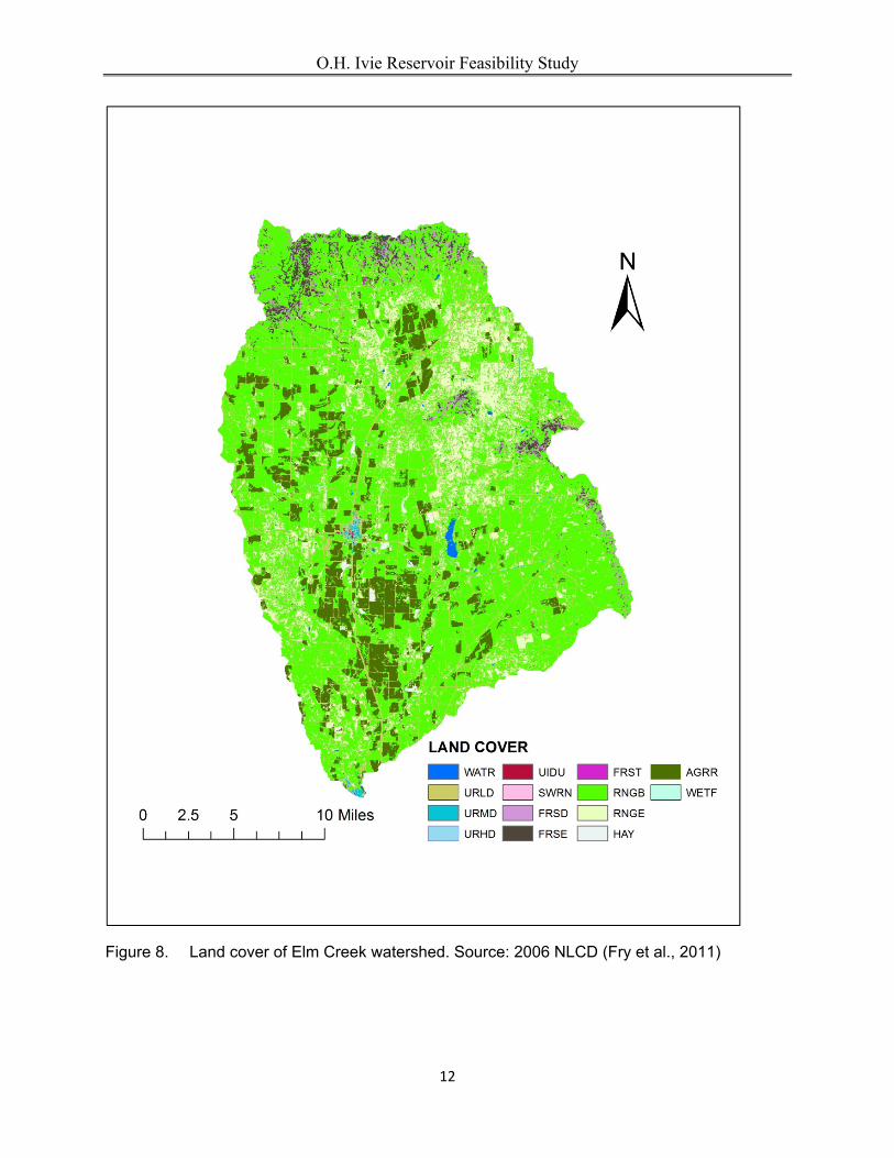
The land cover data for HRU development was obtained from the National Land Cover Dataset (NLCD) for year 2006 (Fry et al., 2011). The 2006 NLCD was selected to represent the average land cover over the simulated time period of 1995-2010 (Figure 8). Comparisons of the 2001, 2006, and 2011 NLCDs for Elm Creek indicated no major land use changes for the three periods. From the 2006 NLCD the dominate land cover in the watershed was indicated to be brushy rangeland (RNGB) comprising almost 63 percent of the watershed, followed by grass dominated rangeland (RNGE) at 14 percent, and agricultural row crop at just over 11 percent (Table 2).


10

Table 1. Slope classification description of Elm Creek watershed

Slope Category Area

(acres) Percent of Watershed

(%)

0-1% 107,123 36

1-2% 80,207 27

2-5% 70,111 24

>5% 39,089 13

Figure 6. Slope classification of the Elm Creek watershed


11

Figure 7. SWAT subbasin delineation of Elm Creek watershed


12

Figure 8. Land cover of Elm Creek watershed. Source: 2006 NLCD (Fry et al., 2011)


13

Table 2. Land cover of Elm Creek watershed by classification categories in the 2006 NLCD (Fry et al., 2011)

Land Cover Abbreviation Area

(acres)

Percent of Watershed Area

(%)

Range-Brush RNGB 185,663 62.61

Range-Grasses RNGE 41,534 14.01

Agricultural Land-Row Crops AGRR 33,543 11.31

Residential-Low Density URLD 20,228 6.82

Forest-Evergreen FRSE 6,826 2.30

Forest-Deciduous FRSD 5,312 1.79

Hay HAY 1,527 0.51

Water WATR 771 0.26

Residential-Medium Density URMD 684 0.23

Residential-High Density URHD 176 0.06

Industrial UIDU 76 0.03

Forest-Mixed FRST 75 0.03

Wetlands-Forested WETF 86 0.03

Southwestern US (Arid) Range SWRN 30 0.01

Total ─ 296,531 100.00

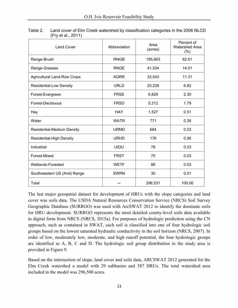
The last major geospatial dataset for development of HRUs with the slope categories and land cover was soils data. The USDA Natural Resources Conservation Service (NRCS) Soil Survey Geographic Database (SURRGO) was used with ArcSWAT 2012 to identify the dominate soils for HRU development. SURRGO represents the most detailed county-level soils data available in digital form from NRCS (NRCS, 2015a). For purposes of hydrologic prediction using the CN approach, such as contained in SWAT, each soil is classified into one of four hydrologic soil groups based on the lowest saturated hydraulic conductivity in the soil horizon (NRCS, 2007). In order of low, moderately low, moderate, and high runoff potential, the four hydrologic groups are identified as A, B, C and D. The hydrologic soil group distribution in the study area is provided in Figure 9.

Based on the intersection of slope, land cover and soils data, ARCSWAT 2012 generated for the Elm Creek watershed a model with 29 subbasins and 387 HRUs. The total watershed area included in the model was 296,500 acres.


14

Figure 9. Hydrologic soil groupings for Elm Creek watershed based on SURGO level data.


15

O.H. Ivie Reservoir Basin SWAT Model Development

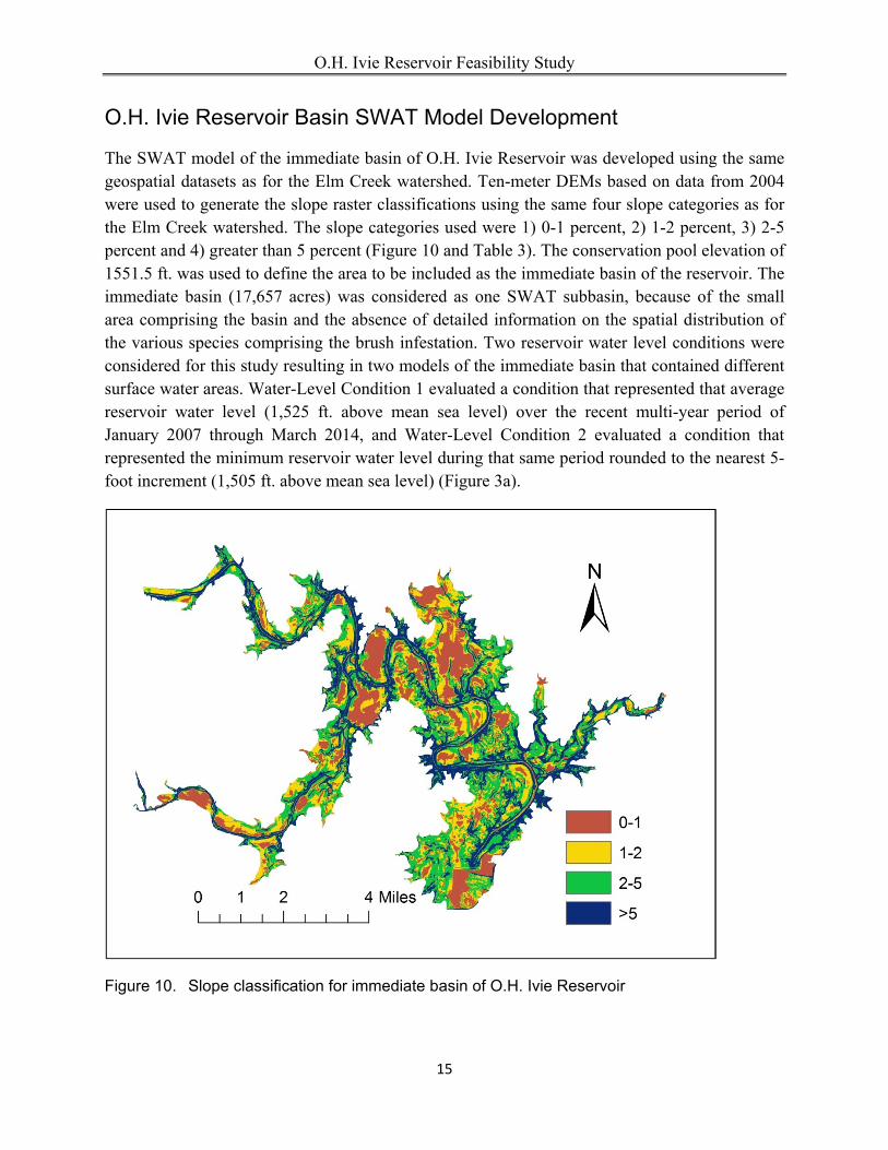
The SWAT model of the immediate basin of O.H. Ivie Reservoir was developed using the same geospatial datasets as for the Elm Creek watershed. Ten-meter DEMs based on data from 2004 were used to generate the slope raster classifications using the same four slope categories as for the Elm Creek watershed. The slope categories used were 1) 0-1 percent, 2) 1-2 percent, 3) 2-5 percent and 4) greater than 5 percent (Figure 10 and Table 3). The conservation pool elevation of 1551.5 ft. was used to define the area to be included as the immediate basin of the reservoir. The immediate basin (17,657 acres) was considered as one SWAT subbasin, because of the small area comprising the basin and the absence of detailed information on the spatial distribution of the various species comprising the brush infestation. Two reservoir water level conditions were considered for this study resulting in two models of the immediate basin that contained different surface water areas. Water-Level Condition 1 evaluated a condition that represented that average reservoir water level (1,525 ft. above mean sea level) over the recent multi-year period of January 2007 through March 2014, and Water-Level Condition 2 evaluated a condition that represented the minimum reservoir water level during that same period rounded to the nearest 5-foot increment (1,505 ft. above mean sea level) (Figure 3a).

Figure 10. Slope classification for immediate basin of O.H. Ivie Reservoir


16

Table 3. Slope classification description for immediate basin of O.H. Ivie Reservoir

Slope Category Area

(acres) Percent of Watershed

(%)

0-1% 3,551 20.1

1-2% 3,948 22.4

2-5% 5,537 31.4

>5% 4,621 26.1

The land cover data for HRU development was obtained from the 2006 NLCD (Fry et al., 2011). Much of the immediate basin was, however, represented as water due to the higher reservoir water levels at the time the 2006 NLCD was developed. For both Water-Level Condition 1 and 2, all exposed land surface not included in the 2006 NLDC was considered as having become brush infestation. As with the Elm Creek model, the 2006 NLCD with the above modification to define brush infestation was used to represent the average land cover over the simulated time period of 1995-2010. Based on visual observations at key observations points around the lake, Mr. Chuck Brown, Director of Operations at the Upper Colorado River Authority, estimated that 60 percent of the brush infestation of the O.H. Ivie Reservoir basin was comprised of saltcedar, 35 percent of willow baccharis and 5 percent of mesquite (Brown, 2014).1 The land cover for Water-Level Condition 1 is provided in Figure 11 and Table 4. For Water-Level Condition 1 the major land cover was water at 49 percent followed by the brush infestation category (BRUSH) at 45 percent with a mix of land covers constituting the remaining 6 percent. For Water-Level Condition 2 the BRUSH category dominates at 74 percent of the immediate basin, followed by water at 20 percent and again a mix of land covers comprising the remaining 6 percent (Figure 12 and Table 5). Note that the urban land covers in the immediate basin are largely service roads and boat ramp areas, which comprise only a small amount of the area.

Because the digital NRCS SURRGO database (NRCS, 2015a) only defined a single soil referred to as “Water” for much of the immediate basin, a second approach was employed to develop the needed soils. The approach taken to develop the distribution of soils in the immediate basin of O.H. Ivie Reservoir was to obtain paper copies of soil surveys for the three counties that partially occur in the immediate basin (Wiedenfeld et al., 1970; Botts et al., 1974; Clower and Dowell, 1988). The relevant soil maps in each survey were georeferenced and the soils were delineated into a digital format using GIS manipulations to create an equivalent SURRGO-level soils map (see Figure 13 for soils of immediate basin by hydrologic soil groups). This digital soils data map was then used in ArcSWAT 2012 with the slope and land cover databases in HRU development.

1 The visual observations of Mr. Brown at the Upper Colorado River Authority represent the best available information on the brush infestation in the immediate basin. Such traditional sources of brush infestation data, as the Texas Parks and Wildlife Department’s Ecological Systems Classification (Elliot et al., 2014), provided no indication of brush infestation in this area despite the obvious presence of such in recent years.


17

Figure 11. Land cover for Water-Level Condition 1 of immediate basin of O.H. Reservoir. (Brush is area of saltcedar, willow baccharis and mesquite infestation.)

Table 4. Land cover for Water-Level Condition 1 of immediate basin of O.H. Reservoir. (Brush is area of saltcedar, willow baccharis and mesquite infestation.)

Land Cover Abbreviation Area

(acres) Percent of Area

(%) Water WATR 8,564 48.50

Brush Infestation BRUSH 7,986 45.23

Forest-Evergreen FRSE 592 3.35

Residential-Low Density URLD 185 1.05

Hay HAY 115 0.65

Agricultural Land-Row Crops AGRR 109 0.62

Forest-Deciduous FRSD 44 0.25





Total ─ 17,657 100.00


18

Figure 12. Land cover for Water-Level Condition 2 of immediate basin of O.H. Reservoir. (Brush is area of saltcedar, willow baccharis and mesquite infestation.)

Table 5. Land cover for Water-Level Condition 2 of immediate basin of O.H. Reservoir. (Brush is area of saltcedar, willow baccharis and mesquite infestation.)

Land Cover Abbreviation Area (acres) Percent of

Watershed Area (%)

Brush Infestation BRUSH 13,027 73.78

Water WATR 3,523 19.95

Forest-Evergreen FRSE 592 3.35

Residential-Low Density URLD 185 1.05

Hay HAY 115 0.65

Agricultural Land-Row Crops AGRR 109 0.62

Forest-Deciduous FRSD 44 0.25





Total ─ 17,657 100.00


19

It is important to note that the area in each modeled condition represented by the “water” land cover category is non-contributing to the water yield hydrologic components of the SWAT model.

Based on the intersection of slope, land cover and soils data, ArcSWAT 2012 generated for the single subbasin a Water-Level Condition 1 model containing 74 HRUs of which 26 HRUs were water and a Water-Level Condition 2 model containing 75 HRUs of which 27 HRUs were water.

Figure 13. Hydrologic soil groupings for immediate basin of O.H. Ivie Reservoir based on SURGO level data obtained from county soil survey reports.


20

Temporal Model Input In addition to the geospatial data requirement to develop the SWAT models, there are temporal data needs to operate the model. The main temporal data needs are land management and daily streamflow, precipitation, wind, solar radiation, and minimum and maximum air temperature data. Temporal data for operating the model were needed for the period of 1993-2010, which allowed for a two-year period of model operation to overcome any inaccuracies in the model-assumed initial conditions prior to comparing simulations to observed streamflows for the period of 1995-2010.

As discussed above under the section on Modeling Approach, the source of the daily streamflow data for model calibration was the USGS gaging station 08127000 on Elm Creek near Ballinger, Texas. The daily streamflow data for the period January 1, 1995 through December 31, 2010 were obtained from USGS (2015b). Additional information provided by the USGS on the quality of the daily streamflow data indicated that records are good above 5 cubic feet per second (cfs) and poor below that flow (USGS, 2015c).

Data on municipal withdrawals from Lake Winters were obtained from the Texas Commission on Environmental Quality online water rights database (TCEQ, 2014). These data were manipulated into the proper units and added as input to SWAT to characterize Lake Winters.

The precipitation data are an extremely important input to the model. Because of the high spatial and temporal variability of precipitation and the distance between precipitation monitoring stations, these data are typically the source of some of the discrepancies between simulated and observed streamflows when calibrating the SWAT model. Especially for relatively small watersheds, such as Elm Creek, where the hydrologic response is not integrated over large areas and multiple precipitation measurement locations, the unrepresentativeness of recorded precipitation data to actual precipitation can constrain the ability to calibrate the model. For this study the precipitation data were obtained from NRCS High-resolution Climate Extractor (HCE) for the period of 1993-2006, with 2006 being the most recently available data from that source, and Oregon State Prism Data for 2007 through 2010 (NRCS, 2015b; PRISM, 2014). Both data sources provide spatially-distributed, serially complete precipitation data. The reason for selecting this combined source of data will be discussed in the next section (Elm Creek Watershed Model Calibration).

The required daily maximum and minimum air temperature data, wind, relative humidity and solar radiation for both the Elm Creek watershed and immediate basin of O.H. Ivie Reservoir were downloaded data from Global Weather Data for SWAT (http://globalweather.tamu.edu/). The weather data from this online resource was developed to obtain SWAT weather data extracted from the National Centers for Environmental Prediction Climate Forecast System Reanalysis, which was designed and executed as a global, high resolution data source.


21

Information on the management practices used on the cropland and on rangeland regarding management and stocking densities in the Elm Creek watershed was obtained from personal communication with Texas A&M AgriLife Extension Service personnel in Runnels County, Texas (AgriLife, 2014).

Elm Creek Watershed Model Calibration

Calibration Process The Elm Creek model was calibrated for hydrology using a combination of automated and manual adjustments of process-related input parameters. These input parameters were adjusted to minimize the differences between the simulated and observed (also referred to as measured) daily flows at USGS station 08127000, represented as the outlet of the SWAT model. Parameters were varied within their acceptable ranges as described in the SWAT input and output documentation (Neitsch et al., 2011). A combination of graphical comparisons of simulation and observational data and statistical measures were used to evaluate goodness-of-fit. The graphical comparisons consisted of time-series and scatter plots of monthly and annual data. Time-series and scatter plots of daily data were also used in the calibration process. But by nature of the daily time step and daily precipitation input data of SWAT, the daily results were used only to guide the calibration to observed monthly and annual streamflow.

Four statistical measures of goodness-of-fit were considered: mean, percent bias (PBIAS), Nash-Sutcliffe coefficient of model efficiency (NSE), and the ratio of root mean square error (RMSE) to the standard deviation of the observational data (RSR) (Moriasi et al., 2007). Each is calculated as follows:

Mean

n

i

obsi

obs nYY1

/ or

n

i

simi

sim nYY1

/

Percent Bias

n

i

obsi

n

i

simi

obsi

Y

YYPBIAS

1

1

Nash-Sutcliffe Efficiency

n

i

n

i

obsobsi

simi

obsi YYYYNSE

1 1

22/1


22

RMSE-observation standard deviation ratio

2

1

2

1

n

i

obsobsi

n

i

simi

obsi

YY

YY

RSR

Where

obsiY = the observed streamflow on the ith period (day, month, year),

sim

iY = the simulated streamflow on the ith period (day, month, year),

Y = the mean of the observed or simulated streamflow for 1995-2010, and

n = total number of periods or time steps (days = 5,844, months = 192, year = 16)

The Y is a simple statistical measure of central tendency of the simulated and observed data. The

closer the simulated and observed Y flow, the better the fit of the model.

PBIAS is a measure of the average tendency of the simulated data to be larger or smaller than the observational data. The optimal value of PBIAS is 0.0, with low-magnitude values indicating more accurate model simulation than higher values. Positive values of PBIAS indicate the model is generally under predicting flow, and negative values indicate the model is over predicting flow. Based on Moriasi et al. (2007), the following PBIAS values were used to evaluate model goodness-of-fit for monthly and yearly time steps: between 0 and plus or minus (+/-) 10 percent indicates a “very good” model simulation fit to observed flows, values between +/-10 and +/-15 percent indicates a “good” model simulation fit, and values between +/-15 and +/-25 percent indicates a “satisfactory” model simulation fit.

NSE is a measure of the plotted fit of observed verses simulated data to the 1:1 line (Moriasi et al., 2007). The NSE can range from -∞ to 1.0 with a value of 1.0 indicating a perfect fit between simulated and observed data. An NSE of 0 indicates that the model predictions are as accurate as the mean of the observed data, and an NSE of less than 0 indicates that the observed mean is a better predictor than the model. Based on Moriasi et al. (2007), the following NSE values were used to evaluate model goodness-of-fit for monthly and yearly time steps: 0.75 < NSE ≤ 1.00 indicates a “very good” model simulation fit to observed flows, 0.65 < NSE ≤ 0.75 indicates a “good” model simulation fit, and 0.50 < NSE ≤ 0.65 indicates a “satisfactory” model simulation.

RSR standardizes the commonly used error index statistic of RMSE by the standard deviation of the observed data. Consequentially RSR contains the benefits of an error index statistics and a normalization factor (Moriasi et al., 2007). RSR values range from an optimal value of 0, which indicates zero residual variation and perfect model simulation, to a large positive value, which indicates poor model simulation. The lower RSR the better the model simulation performance. Again, based on Moriasi et al. (2007), the following RSR values were used to evaluate model


23

goodness-of-fit for monthly and yearly time steps: 0.00 < RSR ≤ 0.50 indicates a “very good” model simulation fit to observed flows, 0.50 < RSR ≤ 0.60 indicates a “good” model simulation fit, and 0.60 < RSR ≤ 0.70 indicates a “satisfactory” model simulation fit.

Reported watershed hydrologic studies provide NSE values more consistently than either PBIAS or RSR. A sense of the level of statistical goodness-of-fit obtained in some Texas watershed applications of SWAT can be obtained from this non-exhaustive overview of some published studies and the NSE values reported for these studies. For the 1,432 sq. mi. Guadalupe River watershed above Canyon Lake, Bumgarner and Thompson (2012) reported NSE values of 0.72 for the daily SWAT flow simulation comparison to observational data and a value of 0.85 for the monthly simulation. Moon et al. (2004) applied SWAT to the 600 sq. mi. Cedar Creek watershed of East Texas and reported NSE values of 0.48 and 0.78 for daily and monthly simulation evaluations. For the 653 sq. mi. watershed of the Arroyo Colorado, Kannan et al. (2011) reported NSE values ranging from a low of 42 to a high of 60 based on SWAT simulated daily streamflows compared to observational data at two gages and for separate calibration and validation periods. Saleh and Du (2004) reported calibration and validation NSE values of 0.17 and 0.62 for SWAT simulation of daily flows for the 356 sq. mi. Upper North Bosque River watershed and NSE values of 0.50 and 0.78 for monthly flow simulations. In a separate study of the entire Bosque River watershed, Santhi et al. (2001) reported NSE values ranging from 0.62 to 0.89 for separate calibration and validation time periods comparing SWAT monthly simulations to observation data at two gage locations. For the 140 sq. mi. North Fork Guadalupe River watershed, Afinowicz et al. (2005) reported NSE values of 0.40 and 0.09 for calibration and validation of SWAT simulated daily streamflows and 0.20 and 0.50 for calibration and validation of monthly streamflows. From these reported studies in Texas, two general patterns emerge that are not without exception. Monthly NSE values are usually better (higher) than the daily values, and reported applications of SWAT to larger watersheds produce higher NSE values than for smaller watersheds.

Calibration Results

The parameters adjusted during the hydrologic calibration process for the Elm Creek watershed SWAT model are provided in Table 6. Default values were used for all other SWAT process-related input parameters as described in Neitsch et al. (2011). Based on conversation with Mr. Mizenmayer of AgriLife (AgriLife, 2014), the CNs for rangeland were varied between the two periods of 1995-1999 and 2000-2010. The initial attempts at model calibration indicated different hydrologic responses to precipitation for these two periods that could not be resolved using one set of prescribed CNs for the entire calibration period. Mr. Mizenmayer stated that appreciably higher stocking densities of cattle occurred prior to the short, but intense drought that started in 1998, peaked in 1999, and persisted through mid-2000. Further, Mr. Mizenmayer provided the following overview of recent conditions in Runnels County and the watershed area. As a result of the drought, several large ranches in the watershed greatly reduced or entirely


24

eliminated their herd sizes and a watershed-wide embracing of this same strategy was necessitated. The continuation of various levels of drought in the watershed for 2000-2010, as also indicated by O.H. Ivie Reservoir water levels (Figure 3), resulted in diminished herd sizes until restocking has gradually occurred within recent years beyond the end of the calibration period in 2010. To account for this substantive change in stocking densities and runoff response for this dominate watershed land cover (see Table 2), CNs were increased 10 percent above default values for the 1995-1999 period over the CNs for the remainder of the calibration period and decreased by 5 percent after 1999, guided by typical CNs for agricultural lands and their variations based on ground cover and grazing intensities as provided in NRCS (1986). The daily calculation of CNs was based on plant evapotranspiration, which was accomplished by setting SWAT input parameter ICN = 1.

Table 6. Process-related parameters adjusted in calibration of SWAT Elm Creek model.

Parameter Description (units) SWAT input file location

Calibrated parameter value

Default parameter value

ALPHA_BF Base-flow recession constant (days)

*.gw 0.07 0.048

CANMX Maximum canopy storage (mm) *.hru 5 **

CN2 Initial SCS curve number [for 1995-1999 grazing conditions] (--)

*.mgtAll Rangeland

increased by 10% of original CN2

**

CNOP SCS runoff curve number for management operations [for 2000-2010 grazing conditions] (--)

*.mgtAll Rangeland

decreased by 5% of original CN2

**

ESCO Soil evaporation compensation factor

*.hru 0.4 0.95

GW_DELAY Groundwater delay time (days) *.gw 30 30

GW_REVAP Represents water movement from the shallow aquifer to the root zone (--)

*.gw 0.08 0.02

GWQMN Threshold depth for water in the shallow aquifer for return flow to occur (mm)

*.gw 90 0

ICN Daily curve number calculation Method

*.bsn 1 0

RCHRG_DP Deep aquifer percolation factor (--) *.gw .85 0

REVAPMN Threshold depth for water in the shallow aquifer for percolation to the deep aquifer to occur (mm)

*.gw 90 1

SHALLST Initial depth of water in shallow aquifer (mm H2O)

*.gw 80 1000

SOL_AWC Available water capacity of the soil layer (mm water/mm soil)

*.sol +0.03 **

SURLAG Surface runoff lag coefficient (--) .bsn 1 4


25

In Table 7 is provided a summary of the calibration results and statistical measures of goodness-of-fit. Plots of simulated and observed flow at the outlet of Elm Creek watershed are provided on a monthly basis in Figures 14 and 15 and on a yearly basis in Figures 16 and 17.

Figure 14. Time series of measured and simulated monthly streamflow for Elm Creek

watershed, 1995-2010.

Figure 15. Scatter plot of measured and simulated monthly streamflow for Elm Creek

watershed, 1995-2010.


26

Figure 16. Time series of measured and simulated annual streamflow for Elm Creek watershed, 1995-2010.

Figure 17. Scatter plot of measured and simulated annual streamflow for Elm Creek watershed, 1995-2010.


27

Table 7. Hydrologic calibration statistics and results of SWAT Elm Creek model.

Calibration time step

Percent bias (PBIAS) %

Coefficient of determination

(R2)

RMSE-observation

standard deviation ratio

(RSR)

Nash-Sutcliffe coefficient of

model efficiency (NSE)

Daily -1.0 0.44 0.75 0.44

Monthly -1.0 0.76 0.50 0.75

Yearly -1.0 0.65 0.59 0.65

Calibra-tion time

step

Simulated

Measured

Max stream-

flow (cfs)

Min stream-

flow (cfs)

Mean stream-

flow (cfs)

Median stream-

flow (cfs)

Max stream-

flow (cfs)

Min stream-

flow (cfs)

Mean stream-

flow (cfs)

Median stream-

flow (cfs)

Daily 6,032 0 31 2 12,400 0 30 2

Monthly 799 0 31 7 770 0 31 4

Yearly 88 3 31 16 96 1 30 16

Model Calibration Discussions

The calibration of the Elm Creek watershed model proved to be challenging. The initial calibration efforts quickly exposed deficiencies in the precipitation data from the datasets associated with the SWAT model. While a modicum of improvement was realized from using data from individual precipitation monitoring locations available online from the National Oceanic and Atmospheric Administration (NOAA), the simulated flow patterns still indicated weaknesses in the input precipitation data that prevented reasonable simulation of runoff during several wet periods wherein the predicted flows were inconsistently either too high or too low. Use of the HCE precipitation data, which were available through 2006, and PRISM data for the remainder of the period improved model simulated runoff response to precipitation events. Even with the improvement in simulated flow with these precipitation data, the high observed streamflow month of June 1997 was still grossly under predicted (Figures 14 and 15) and this under prediction led to the same issue with the annual predictions for year 1997 (Figure 16 and 17).

However, with the HCE-PRISM precipitation data and the rangeland CN adjustments to reflect changes in stocking densities resulting from the drought centered around 1999, acceptable goodness-of-fit statistics were obtained for the monthly and annual calibration steps and simulated and measured mean flows were in good agreement (Table 7). As anticipated, the statistical measures were better for the monthly time periods than for the daily data. Somewhat unusual, the yearly statistical measures were not as good as the monthly, though experience has


28

indicated that this unanticipated result can occur when difficulties arise in predicting some high flow months as occurred for this situation. Based on the measures of goodness-of-fit in Moriasi et al. (2007), the monthly and yearly statistics indicated model performance ranged from the “satisfactory” to “good” categories. Compared to published studies in Texas for comparably sized watersheds, the statistical measures for Elm Creek watershed indicated an acceptably calibrated model.

The calibration parameters developed for the Elm Creek watershed model are expected to readily transfer to the models of the immediate basin of O.H. Ivie Reservoir. The two different modeled areas are within reasonable proximity with the outlet of the Elm Creek watershed being about 20 miles northwest of the central area of the reservoir (Figure 9). Because the dominate land covers in the Elm Creek watershed were brushy rangeland and grassy rangeland, SWAT input process-related parameters were calibrated to the brush replacement or removal conditions to be simulated for the immediate basin of O.H. Ivie Reservoir. The hydrologic soil groups of both watersheds are similar, though estimates of the distribution of the soil groups indicated that Groups A and D soils were both more abundant in the immediate basin than in the Elm Creek watershed, as visually discernible in Figure 9.

One weakness of the modeling effort is that the Elm Creek watershed did not contain areas of intensive infestation of saltcedar and willow baccharis, so these pertinent species were not contained in the model calibration. The simulation of the pre-treatment brush infestation situation of the immediate basin was, therefore, based on the plant growth parameters provided through the expertise of Dr. Kiniry at the U.S. Department of Agriculture – Agricultural Research Service – Grassland, Soil and Water Research Laboratory and the process-related input parameters developed for the SWAT Elm Creek watershed model. Note regarding the transfer of input CNs: the CNs used for rangeland for the period of 2000-2010, which reflected low stocking conditions, were used for the immediate basin as it was anticipated that stocking densities would be light to none for the immediate basin.

A second weakness of SWAT regards its limited capabilities to accurately simulate the hydrologic interconnection of the surface waters in O.H. Ivie Reservoir to adjacent areas of both shallow groundwater and deeper, water saturated soil layers sustained by the reservoir’s surface waters. As strongly suggested by the presence of dense stands of saltcedar and willow baccharis in the exposed reservoir basin, these phreatophytic species likely have roots reaching shallow groundwater zones and soil saturation zones, which are in turn sustained by the water in the reservoir. Through evapotranspiration the phreatophytes remove water from these subsurface zones that would not be reached by shallower rooted grasses. Because of the density of the stands of saltcedar and willow baccharis in the immediate basin, these phreatophytes would also result in increased evapotranspiration exceeding that of other types of brush and tress species that may have roots that grow deep enough to reach these subsurface zones of water but would not grow in such densities and consequently do not have as much leaf area index for evapotranspiration. Under this situation, the subsurface water losses through phreatophytic


29

evapotranspiration would be replaced by water in O.H. Ivie Reservoir. Thus, the phreatophytes exert subsurface water losses not directly incorporated into the SWAT model.

A means of operating SWAT through its auto-irrigation feature is discussed in Appendix A. This feature was used to give a reasonable upper limit on the water salvage realized by a non-phreatophytic replacement vegetation, such as shallower rooted grasses or grass with sparse brush that does not use as much water from the saturation zones, which are anticipated to lie below parts of the immediate basin. Because there are no direct data for O.H. Ivie Reservoir supporting the likely, but spatially limited occurrences of areas for water salvage, this addition to water yield is not directly included in the main body of this report, but provided as an appendix.

Simulation of Effects of Brush Management To evaluate increases in water yield from brush control, SWAT was operated for the condition with the infestation of saltcedar, willow baccharis and mesquite and the water yield for that scenario was compared to the water yield for the condition where these phreatophytic brush species were removed and replaced with another vegetative cover, which was assumed to be grass dominated rangeland.

Simulation Methods Because of the absence of any hydrologic calibration data for the immediate basin of O.H. Ivie Reservoir, the SWAT input parameters developed for the Elm Creek watershed calibration were used in the two O.H. Ivie Reservoir basin models. The two subbasin configurations vary in the amount of the basin that is covered by the remaining water in O.H. Ivie Reservoir. Water-Level Condition 1 incorporates conditions of a reservoir level of 1,525 feet with 7,986 acres of exposed basin with brush infestation. Water-Level Condition 2 incorporates conditions of a reservoir level of 1,505 feet with 13,027 acres of exposed basin with brush infestation. (The exact amount of brush infestation is unknown, but as shown on the Cover Photograph and Figure 1 much of the exposed basin is covered by dense infestations of saltcedar and willow baccharis.) The crop parameters to represent saltcedar in SWAT were taken from the ALMANAC (Agricultural Land Management Alternative with Numerical Assessment Criteria) simulation model and the existing SWAT crop parameters for mesquite were used to represent willow baccharis; both based on the guidance and expertise of Dr. James Kiniry, Research Agronomist at the U.S. Department of Agriculture – Agricultural Research Service – Grassland, Soil and Water Research Laboratory obtained via email communications with Dr. Mike White and Ms. Amber Williams at the same research facility (White and Williams, 2014).

Standard Brush Control Evaluation Method The standard method of evaluating water yield increase from brush control entails operating the SWAT model for conditions with and without the brush infestation and comparing the water


30

yield results from the two simulations. Both SWAT representations of the immediate basin of O.H. Ivie Reservoir were operated for the brush infestation conditions using the information described above and locally-specific precipitation data from HCE for 1993-2006 and PRISM for 2007-2010 (NRCS, 2015b; PRISM, 2014). Each water-level condition was operated in SWAT with the brush infestation land cover for the period of 1995-2010 with the simulation actually starting in January 1, 1993 to allow two years for the model to equilibrate after initial conditions were specified at model start-up. The water level in the reservoir was held constant over the simulated period. These SWAT simulations were considered the baseline condition to which brush removal simulations would be compared.

To simulate the removal of saltcedar, willow baccharis and mesquite for Water-Level Conditions 1 and 2, all invasive brush was replaced with grassy rangeland containing areas dominated by grammanoid or herbaceous vegetation, generally greater than 80 percent of total vegetation (RNGE in the SWAT plant data input file). Thus, 100 percent of the brush infestation was considered as treatable.

To assess changes in water yield from removal of the brush infestation, the baseline and scenarios were compared using the standard water yield output from SWAT.

Water Yield Results The average annual water yield was obtained from SWAT output for the baseline condition with saltcedar, willow baccharis and mesquite present and the two water-level conditions under the grassy brush replacement scenario. For each of these three modeled simulations, the annual average water yield predicted by SWAT was obtained for each of the single subbasin to provide a total annual average water yield. This water yield is taken for the SWAT outputted parameter WYLD in the subbasin output file. WYLD represents the predicted net amount of water that leaves a subbasin that contributes to streamflow via surface runoff, lateral flow and groundwater discharge and does not include losses in a stream reach, such as from evaporation and transmission losses. Because of the immediate proximity of each subbasin HRU to the waters of O.H. Ivie Reservoir, WYLD was considered a more relevant determination of water yield than other SWAT output that would include additional reductions due to evaporation and transmission losses in a conveyance stream. The annual average output for WYLD for the period of 1995-2010 was considered for this study per the feasibility study guidance (TSSWCB, 2014). The difference in water yield between each brush control simulation and the brush infestation baseline simulation was calculated and is summarized in Table 8. Because of the different distributions of hydrologic soil groups determined for Water-Level Condition 1 and 2, the average increase in water yield is different. The exposed land area not under water in Water-Level Condition 1 had a greater percentage of soils in hydrologic groups favoring more runoff, generally greater slopes, than the additionally exposed land area under Water-Level Condition 2 (see Figures10 and 13). This difference in the distribution of hydrologic soil groups resulted in a greater increase in water yield under Condition 1 (29,465 gallons/acre/year [gal/ac/yr]) than


31

under Condition 2 (20,473 gal/ac/yr). All predicted yield increases are well within the range of yield increases predicted in other brush control modeling studies (Connor et al., 2000; Bumgarner and Thompson, 2012).

Table 8. Predicted increase in water yield from brush control in the immediate basin of O.H. Ivie Reservoir; annual average for 1995-2010.

Water-Level Condition Condition 1 (average-

water level) Condition 2 (low-water

level)

Annual Average Increase in Water Yield per unit area of Brush Control (water depth)

27.56 mm (1.09 inches)

19.15 mm (0.75 inches)

Annual Average Water Yield Increase (million gallons/year for entire basin)

235.3 million gal / year 266.7 million gal / year

Brush Area 7,986 ac 13,027 ac

Annual Average Water Yield 29,465 gal/ac/yr 20,473 gal/ac/yr

A second less quantitative analysis was performed with SWAT that predicted a maximum water salvage from removal of the phreatophytic saltcedar and willow baccharis because of their deep roots that are capable of reaching deeper zones of water saturation that would be unavailable or not as available to the replacement vegetation. This analysis is based on the reasonable assumption that portions of the brush infestation are underlain by zones of saturated soil and shallow groundwater that are hydrologically connected to the water in O.H. Ivie Reservoir. The extra evapotranspiration by the phreatophytic brush from these zones of plentiful water were assumed to be replaced by water from O.H. Ivie Reservoir. Because of the unknowns associated with both the extent of area where this process of enhanced evapotranspiration will occur and temporal permanency of these areas, this additional water savings is not formally included in the evaluation, but rather is left for consideration in Appendix A.

Summary A feasibility study under the TSSWCB WSEP was undertaken for the immediate basin of O.H. Ivie Reservoir. The study was performed through funding of the TSSWCB with the Upper Colorado River Authority (UCRA) as the lead performing entity and the Texas Institute for Applied Environmental Research (TIAER) the performing entity of the computer modeling development and application. The TSSWCB WSEP requires that a feasibility study be performed using computer models to predict water yield changes for any watershed where brush control is being considered. Due to an extended period of low water level in O.H. Ivie Reservoir, a large amount of the immediate basin of the reservoir has been exposed and phreatophytic brush, predominately saltcedar and willow baccharis, have infested these exposed areas in dense stands. It is the purpose of this study to apply the Soil and Water Assessment Tool (SWAT) to evaluate changes in water yield that could be realized with the replacement of the dense stands of phreatophytic brush with grassy rangeland or brushy rangeland.


32

O.H. Ivie Reservoir is located in west-central Texas near the city of Ballinger. At conservation pool elevation, the reservoir has a storage capacity of 554,000 acre-feet and a surface area of 19,100 acres. Since 1998 O.H. Ivie Reservoir has not had water levels at the conservation pool elevation and within recent years the water levels have fallen to between 30 to almost 50 feet below the conservation pool elevation. Commensurately, reservoir storage has suffered such that within recent years it has consistently remained at less than 20 percent of conservation storage capacity.

In order to properly calibrate SWAT, the Elm Creek watershed was first modeled. The Elm Creek watershed model was defined as the drainage area above the U.S. Geological Survey (USGS) streamflow gaging station on Elm Creek. This watershed was selected as a surrogate for the immediate basin of O.H. Ivie Reservoir for calibration purposes, because of the absence of gaged streamflow records for the immediate basin that precluded direct calibration of the model to the immediate basin. The Elm Creek watershed outlet is located approximately 20 miles northwest of the central portion of O.H. Ivie Reservoir. Also the Elm Creek watershed and immediate basin have similar soils and the dominate land covers. The SWAT model of Elm Creek watershed was calibrated against the streamflow record of the USGS gage for the period of 1995-2010. Through adjustment of process-based input parameters to SWAT, an acceptably calibrated model was obtained based on typical statistical measures of goodness-of-fit. The SWAT simulated daily mean flow of 31 cfs compared favorably to the observed daily mean flow of 30 cfs. Other statistical measures of fit of simulated monthly flows to observed monthly flows were rated to range from “satisfactory” to “good.”

The process-based input parameters from the calibrated Elm Creek watershed model were used in the SWAT models that were developed for the immediate basin of O.H. Ivie Reservoir. Two different immediate basin models were developed reflecting two different water levels in the reservoir. Water Level Condition 1 was based on the average reservoir water elevation of 1,525 ft. above mean seal level over the recent multi-year period of January 2007 through March 2014, and Water Level Condition 2 used the lowest water elevation over that period of 1,505 ft. For both baseline water-level conditions, the distribution of brush was assumed to be 60 percent saltcedar and 40 percent a combination of willow baccharis and mesquite, based on the estimated species distribution of the brush infestation in the immediate basin. Willow baccharis is much more plentiful than mesquite, but both are modeled with the same plant growth parameters in SWAT. Each water-level condition model was operated for the baseline brush infestation scenario and the replacement vegetation for each scenario was grass dominated rangeland (grassy rangeland). For all cases modeled, the period of simulation was 1995-2010.

The increased water yield of 20,000 gal/ac/yr was determined from comparison of water yield results of the baseline brush infestation scenario to the replacement vegetation scenario under each of the two water-level conditions. In SWAT, water yield is the combination of direct runoff, lateral flow and shallow groundwater flow that would reach the water in O.H. Ivie Reservoir.


33

References

Afinowicz, J.D., C.L. Munster, and B.P. Wilcox. 2005. Modeling effects of brush management on the rangeland water budget: Edward Plateau, Texas. J. American Water Resources Assoc. 41(1):181-193.

AgriLife (Texas A&M AgriLife Extension Service). 2014. Telephone conversations over multiple occasions with Mr. Marty Gibbs and Mr. Richard Mizenmayer, Ballinger, Texas (2014-2015).

Arnold, J.G., J.R. Kiniry, R. Srinivasan, J.R. Williams, E.B Haney, and S.L. Neitsch. 2013. Soil and Water Assessment Tool Input/Output Documentation Version 2012. (TR-439). USDA Agricultural Research Service Agricultural Grassland, Soil and Water Research Laboratory and Texas A&M AgriLife Blackland Research Center, Temple, Texas.

Arnold, J.G., R. Srinivasan, R.S. Muttiah, and J.R. Williams. 1998. Large‐area hydrologic modeling and assessment: Part I. Model development. J. American Water Resources Assoc. 34(1): 73-89.

Botts, O.L., B. Hailey, and W.D. Mitchell. 1974. Soil Survey of Coleman County, Texas. United States Department of Agriculture, Soil Conservation Service in cooperation with the Texas Agricultural Station.

Brown, C. 2014. E-mail communication January 17, 2014 regarding brush infestation of O.H. Ivie Reservoir basin. Upper Colorado River Authority, San Angelo, TX.

Bumgarner, J.R. and F.E. Thompson. 2012. Simulation of Streamflow and the Effects of Brush Management on Water Yields in the Upper Guadalupe River Watershed, South-Central Texas, 1995-2010. (Scientific Investigations Report 2012-5051) U.S. Geological Survey.

Clower, D.F. and G.S. Dowell, III. 1988. Soil Survey of Concho County, Texas. United States Department of Agriculture, Soil Conservation Service in cooperation with the Texas Agricultural Station and Texas State Soil and Water Conservation Board.

CRMWD (Colorado River Municipal Water District). 2015. Who is the Colorado River Municipal Water District? Website. <http://www.crmwd.org/crmwd_district.htm>. Accessed November 2, 2015.

Connor, J.R., J. Bach, B. Dugas, R. Muttiah, W. Rosenthal, S. Bednarz, and T. Dybala. 2000. Brush Management/Water Yield Feasibility Studies for Eight Watersheds in Texas. (TR-182). Texas Water Resources Institute, Texas A&M University, College Station, Texas.

Elliott, Lee F., David D. Diamond, C. Diane True, Clayton F. Blodgett, Dyan Pursell, Duane German, and Amie Treuer-Kuehn. 2014. Ecological Mapping Systems of Texas: Summary Report. Texas Parks and Wildlife Department, Austin, Texas. (Geospatial data available at: <https://tpwd.texas.gov/gis/data>. Accessed November 13, 2015.)

Fry, J., Xian, G., Jin, S., Dewitz, J., Homer, C., Yang, L., Barnes, C., Herold, N., and Wickham, J. 2011. Completion of the 2006 National Land Cover Database for the Conterminous United States, PE&RS, Vol. 77(9):858-864. Available online at: < http://www.mrlc.gov/nlcd2006.php>

Gregory, L. and W. Hatler. 2008. A Watershed Protection Plan for the Pecos River in Texas. Texas A&M University AgriLife Research and Extension and Texas Water Resources Institute.


34

Hatler, W.L. and C.R. Hart. 2009. Water Loss and Salvage in Saltcedar (Tamarix spp.) Stands on the Pecos River, Texas. Invasive Plant Science and Management 2:309-317.

Holmes, D.M. 1998. Management and Ecology of Willow Baccharis in the Texas Rolling Plains. Master of Science Thesis, Range Science, Texas Tech University, Lubbock, TX.

Jones, C.A. and L. Gregory. 2008. Effects of Brush Management on Water Resources. (TR-338). Texas Water Resources Institute, Texas A&M AgriLife, College Station, Texas.

Kannan, N., J. Jeong, R. Srinivasan. 2011. Hydrologic Modeling of a Canal-Irrigated Agricultural Watershed with Irrigation Best Management Practices: Case Study. ASCE Journal of Hydrologic Engineering. 16(9):746-757.

Larkin, T.J. and G.W. Bomar. 1983. Climatic Atlas of Texas. (LP-192). Texas Department of Water Resources. Austin, Texas.

McDaniel, K.C. 2015. Saltcedar Information. Available online from Weed Information New Mexico State University at <http://age-web.nmsu.edu/saltcedar/Index.htm>. Accessed March 6, 2015.

McLendon, T., C.R. Pappas, C.L. Coldren, E.B. Fish, M.J. Beierle, A.E. Hernandez, K.A. Rainwater, and R.E. Zartman. 2012. Application of the EDYS Decision Tool for Modeling of Target Sites [in Gonzales County] for Water Yield Enhancement through Brush Control. KS2 Ecological Field Service, LLC and Texas Tech University.

Moriasi, D.N., J.G. Arnold, M.W. Van Liew, R.L. Bingner, R.D. Harmel, and T.L. Veith. 2007. Model evaluation guidelines for systematic quantification of accuracy in watershed simulations. Transactions of the American Society of Agricultural and Biological Engineers, 50 (3), 885-900.

Moon, J., R. Srinivasan, and J.H. Jacobs. 2004. Stream flow estimation using spatially distributed rainfall in the Trinity River Basin, Texas. Transactions of the American Society of Agricultural Engineers. 47(5): 1445-1451.

Neitsch, S.L., J.G. Arnold, J.R. Kiniry, and J.R. Williams. 2011. Soil and Water Assessment Tool Theoretical Documentation: Version 2009. USDA Agricultural Research Service Agricultural Grassland, Soil and Water Research Laboratory and Texas A&M AgriLife Blackland Research Center, Temple, Texas.

NOAA (National Oceanic and Atmospheric Administration). 2015. Concho Park Ivie Reservoir Station, Texas (GHCND: USC00411934). Available online at: <http://www.ncdc.noaa.gov/cdo-web/datasets >

NRCS (Natural Resources Conservation Service). 1986. Urban Hydrology for Small Watersheds (TR-55). U.S. Department of Agriculture.

NRCS (Natural Resources Conservation Service). 2007. Chapter 7 Hydrologic Soil Groups of Part 630 Hydrology National Engineering Handbook. U.S. Department of Agriculture.

NRCS (Natural Resources Conservation Service). 2009. Conservation Practice Standard Code 314 Brush Management. U.S. Department of Agriculture.

NRCS (Natural Resources Conservation Service). 2015a. Soil main website. Available online at: <http://www.nrcs.usda.gov/wps/portal/nrcs/site/soils/home/>


35

NRCS (Natural Resources Conservation Service). 2015b. High-resolution Climate Extractor. Available online at: <http://199.133.175.81/HCEWebT/>

PRISM Climate Group at Oregon State University. 2014. PRISM Products Matrix. Available online at: <www.prism.oregonstate.edu>

Rainwater, K.A., E.B. Fish, R.E. Zartman, C.G. Wan, J.L. Schroeder, and W.S. Burgett. 2008. Evaluation of the TSSWCB Brush Control Program: Monitoring Needs and Water Yield Enhancement. Texas Tech University Water Resources, Lubbock, Texas.

Robinson, T.W. 1958. Phreatophytes. Geological Survey Water-Supply Paper 1423, United States Government Printing Office, Washington, D.C. Available online at <http://pubs.usgs.gov/wsp/1423/report.pdf>

Saleh, A. and B. Du. 2004. Evaluation of SWAT and HSPF within BASINS program for the Upper North Bosque River watershed in Central Texas. Transactions of the American Society of Agricultural Engineers. 47(4): 1039-1049.

Santhi, C., J.G. Arnold, J.R. Williams, W.A. Dugas, R. Srinivasan, and L.M. Hauck. 2001. Validation of the SWAT model on a large river basin with point and nonpoint sources. Journal of the American Water Resources Association. 35(5): 1169-1188.

SCS (Soil Conservation Service). 1986. Urban Hydrology for Small Watersheds. Technical Release 55. U.S. Department of Agriculture – Natural Resources Conservation Service – Conservation Engineering Division. (First issued 1975, Revised 1986). Accessed February 12, 2015. </ftp.wcc.nrcs.usda.gov/wntsc/H&H/other/TR55documentation.pdf>.

TCEQ (Texas Commission on Environmental Quality). 2014. Water Rights Database and Related Files: Water Use data for 1990-1999 and 2000-2013. Available online at: <http://www.tceq.texas.gov/permitting/water_rights/wr_databases.html>

TSSWCB (Texas State Soil and Water Conservation Board). 2011. Excel file containing characteristics of PL-566 reservoirs.

TSSWCB (Texas State Soil and Water Conservation Board). 2014. Policy on Brush Control Feasibility Studies for the Water Supply Enhancement Program (Approved July 18, 2013; Revision Approved May 15, 2014). Texas State Soil and Water Conservation Board, Temple, Texas.

TSSWCB (Texas State Soil and Water Conservation Board). 2015. Water Supply Enhancement Program Website. Accessed January 30, 2015. <http://www.tsswcb.texas.gov/brushcontrol>.

TWDB (Texas Water Development Board). 2014. Lake Winters (Colorado River Basin). Last accessed November 3, 2015. Available online at: <http://www.twdb.texas.gov/surfacewater/rivers/reservoirs/winters/index.asp>

USDA (United State Department of Agriculture) and Texas A&M (Texas A&M University). 2002. Brush Management/Water Yield Feasibility Study for Four Watershed in Texas. (TR-207). Texas Water Resources Institute, Texas A&M University, College Station, Texas.

USGS. (United States Geological Survey). 2015a. USGS National Water Information System: Web Interface for Station 08136600 (O.H. Ivie Reservoir near Voss, TX). Most recently accessed February 7, 2015. <http://waterdata.usgs.gov/tx/nwis/uv?site_no=08136600>.


36

USGS. (United States Geological Survey). 2015b. USGS National Water Information System: Web Interface for Station 08127000 (Elm Creek at Ballinger, TX). Most recently accessed February 13, 2015. < http://waterdata.usgs.gov/tx/nwis/uv?site_no=08127000>.

USGS. (United States Geological Survey). 2015c. USGS National Water Information System: Web Water-Year Summary for Site USGS 08127000. Accessed February 13, 2015. <http://waterdata.usgs.gov/tx/nwis/wys_rpt/?site_no=08127000&agency_cd=USGS>.

White, M. and A. Williams. 2014. Series of email exchanges February 26, 2014 with Dr. Mike White, Agricultural Engineer, and Ms. Amber Williams, Biological Science Technician, U.S. Department of Agriculture – Agricultural Research Service – Grassland, Soil and Water Research Laboratory, Temple, TX.

Wiedenfeld, C.C., L.J. Barnhill, and C.J. Novosad. 1970. Soil Survey of Runnels County, Texas. United States Department of Agriculture, Soil Conservation Service in cooperation with the Texas Agricultural Station.


37

Appendix A

Evaluation Method for Additional Water Savings The predicted water yield increases from the standard analysis using SWAT do not include additional water savings that would be anticipated from water salvage. For the purposes of this study, water salvage was defined as water savings related to reduced losses from the waters of the reservoir resulting from replacement of deep-rooted phreatophytes with shallower rooted vegetation that does not as readily reach a zone of saturation. As further explanation, Hatler and Hart (2009) analyzed diurnal fluctuations in shallow groundwater interconnected hydrologically to the Pecos River to estimate evapotranspiration from saltcedar and water salvage from chemical treatment of the saltcedar. Hatler and Hart reported annual evapotranspiration losses from saltcedar over their 6-year study to range from 420 millimeters (mm) (1.4 ft.) to 1,180 mm (3.9 ft.) and water salvage after treatment ranging from 31 percent to 82 percent of the evapotranspiration. Hatler and Hart also state that water salvage is dependent upon site-specific environmental conditions, dependent upon the actual replacement vegetation, and short-lived if regrowth treatment of the phreatophytes is not continued. The opportunity for water salvage from brush control of the immediate basin of O.H. Ivie Reservoir can be explained as follows. Because saltcedar, willow baccharis and mesquite are all phreatophytes, there is every expectation from the scientific literature on behavior and characteristics of phreatophytes that the deep roots from the species reside in or near shallow zones of saturation and this root connection to plentiful water results in an enhancement of evapotranspiration losses (e.g., Robinson, 1958; Holmes, 1998; Hatler and Hart, 2009). If this hydrologic situation was not the case, these phreatophytic species would not be so dominantly present in the basin as the saltcedar and willow baccharis, especially, are largely absent from other areas of the study area. These saturation zones are the result of their hydrologic connectivity with the waters in O.H. Ivie Reservoir. Thus, a portion of the evapotranspiration losses from the phreatophytes results from their roots entering or being in close proximity to these shallow saturation zones. Because of the hydrologic connection, waters removed from these saturation zones by evapotranspiration will be replaced by water from O.H. Ivie Reservoir creating an additional loss in the water balance of O.H. Ivie Reservoir. Removal of these deep-rooted phreatophytes will reduce evapotranspiration losses and therefore result in a water savings for O.H. Ivie Reservoir in addition to the water yield increase predicted with the standard brush control evaluation method.

Because of the aforementioned weaknesses in SWAT in representing this type of complex shallow groundwater-surface water interaction, the model was applied to approximate the additional evapotranspiration of the phreatophytes resulting from their roots being in zones of saturation. To estimate these additional evapotranspiration losses, the model was operated for Water-Level Condition 2 (low water level) with and without auto-irrigation of SWAT operational. When auto-irrigation was in operation the trigger for automatic irrigation was


38

initiated by plant water demand when potential plant growth was reduced by 7.5 percent and the source of water was defined as diverted water from an unlimited external water source. The initiation of auto-irrigation at 7.5 percent reduction in potential plant growth is the midpoint of the recommended range of 5 to 10 percent. Operation of SWAT with this input setting resulted in saltcedar evapotranspiration within the range reported in Hatler and Hart (2009) and McDaniel (2015).

To evaluate water salvage, the SWAT output results were evaluated at the HRU level to determine the difference in annual average evapotranspiration between the scenario with auto-irrigation operations, which simulated an unlimited water source connection for the phreatophytes, and without auto-irrigation which represents the baseline scenario for the Standard Brush Control Evaluation Method described in the main body of this report. Since the standard method already included the water yield increase realized from brush control, there would be a double accounting of water savings if the auto-irrigation scenario with phreatophytes was compared to a scenario without auto-irrigation that involved replacement vegetation rather than with the phreatophytes still present.

Additional water savings not captured by the standard SWAT brush control evaluation presented in Table 8 would be anticipated from control of saltcedar and willow baccharis, if the replacement vegetation were non-phreatophytic and not having roots that reached to a zone of saturation. An upper limit on the water salvage from brush control disconnecting the roots of the land cover from an assumed underlying unlimited source of shallow groundwater is provided in Table A-1. These maximum water salvage estimates were obtained through the comparisons of evapotranspiration from the baseline brush infestation scenario to the scenario applying the auto-irrigation feature in SWAT to mimic presence of a plentiful water supply from a zone of saturation fed by water from O.H. Ivie Reservoir. Unfortunately, only an upper limit of the annual average water salvage from removal of saltcedar (1.4 million gallons per acre per year) and willow baccharis (0.65 million gallons per acre per year) can be provided, because the areal extent and temporal permanency of the brush infestation underlain by a shallow zone of saturation within the reach of the roots of the phreatophytic vegetation is unknown.

These enormous water salvage numbers are highly unlikely to be obtained for the entire area of phreatophyte infestation. If such high water salvage potential were actually possible for each acre of infestation, the present evapotranspiration rates, which are based on an interconnection of the shallow groundwater to the water in the reservoir, would have totally dried up O.H. Ivie Reservoir. However, it is reasonable to anticipate that depending on soil types, shallow subsurface geology, topography and proximity to water in the reservoir, there are some areas of the phreatophyte infestation where their removal would result in savings approaching these water salvage amounts, while other areas will approach the other extreme of no water salvage potential. The potential additional savings through water salvage are great though undoubtedly spatially-limited within the present stands of saltcedar and willow baccharis.


39

Table A-1. Predicted maximum water salvage from phreatophyte removal where a shallow zone of saturation is present; annual average for 1995-2010.

Water-Level Condition Saltcedar HRUs Willow Baccharis HRUs

Average Annual Evapotranspiration with Auto-Irrigation (mm of water) 1,916 mm 1,198 mm

Average Annual Evapotranspiration without Auto-Irrigation [Baseline Scenario] (mm of water)

592 mm 585 mm

Maximum Potential Annual-Average Water Salvage with Phreatophyte Removal (mm of water; inches of water)

1,324 mm (52 inches) 613 mm (24 inches)

Maximum Per Acre Potential Annual-Average Water Salvage with Phreatophyte Removal (gal/ac/yr)

1,400,000 gal/ac/yr 650,000 gal/ac/yr

brush control feasibility study for the o.h. ivie ... · brush control feasibility study for the...

Documents