1

May 6, June 21, 2013

Revised September 13, 2013

Brownian  Computation  is  Thermodynamically  Irreversible  

John D. Norton1

Department of History and Philosophy of Science

Center for Philosophy of Science

University of Pittsburgh

Pittsburgh PA 15260

http://www.pitt.edu/~jdnorton

jdnorton@pitt.edu

Brownian computers are supposed to illustrate how logically reversible

mathematical operations can be computed by physical processes that are

thermodynamically reversible or nearly so. In fact, they are thermodynamically

irreversible processes that are the analog of an uncontrolled expansion of a gas

into a vacuum.

Keywords: Brownian computation, entropy, fluctuations, thermodynamics of

computation

1.  Introduction  

The thermodynamics of computation applies ideas from thermal and statistical physics to

physical devices implementing computations. Its major focus has been to characterize the

principled limits to thermal dissipation in these devices. The best case of no dissipation arises

when we use processes that create no thermodynamic entropy. They are thermodynamically

reversible processes in which all driving forces are in perfect balance.

Thermal fluctuations, such as arise through random molecular motions, are not normally

a major consideration in thermodynamic analyses. However, they become decisive in the

1 I thank Laszlo Kish for helpful discussion.

2

thermodynamics of computation. For the thermodynamic dissipation associated with

thermodynamically irreversible processes is minimized by reducing the computational devices to

the smallest scales possible, that is, to molecular scales. Thermal fluctuations now become a

major obstacle to reducing thermodynamic dissipation. Consider a thermodynamic process, such

as a single step of computation in a physical computer, at these molecular scales. In order to

proceed to completion, it must overcome these fluctuations. The problem is serious. It is the

essential idea behind a “no go” result described elsewhere (Norton, 2011, Section 7.4;

forthcoming a; manuscript, Part II). If the process is to proceed to completion with reasonable

probability, it follows quite generally that it must create thermodynamic entropy in excess of k ln

2 per step.

This quantity of entropy, k ln 2, is the minimum amount associated by Landauer’s

principle with the erasure of one bit of information. If each step of a computation must create

more thermodynamic entropy that this Landauer limit, then any debate over the cogency of the

Landauer principle is rendered superfluous. Indeed we have to give up the idea that the minimum

thermodynamic dissipation is determined by the logical specification of the computation. For the

minimum dissipation is fixed by the number of discrete steps in the computational procedure

used, which makes this minimum dependent on the implementation.

The no go result wreaks greatest harm when the computer proceeds with what I shall call

a “discrete protocol” tacitly presumed above. It is the familiar protocol in which the computation

is divided into a series of discrete steps, each of which must be completed before the next is

initiated.

There is an escape from the no go result. Bennett (1973, 1982) and Bennett and Landauer

(1985) have described a most ingenious protocol for computation that minimizes its effects. In

the protocol, called “Brownian” computation, the many logical steps of a complicated

computation are collapsed into a single process thermodynamically. It is done by chaining the

logical steps of the computation into a single process such that random thermal motions carry the

computational device’s state back and forth over the steps in a way that is analogous to the

Brownian motion of a pollen grain in water. No step is assuredly complete until the device

happens to enter a final, dissipative trap state from which it escapes with very low probability.

The no go result still applies to this new, indiscrete protocol, but now the thermodynamic

entropy creation required is merely that required for one step. It can be negligible in the context

3

of a large and complicated computation if that single step really is close to thermodynamic

reversibility. That is the hope. However, it is not realized.

For all the mechanical and computational ingenuity of the devices, the thermodynamic

analysis Bennett provides is erroneous. The devices are described as implementing

thermodynamically reversible computations, or coming close to it, thereby demonstrating the

possibility in principle of thermodynamically reversible computation. In fact the devices are

thermodynamically irreversible. They implement processes that are the thermodynamic analog of

an uncontrolled, irreversible expansion of a one-molecule gas, the popping of a balloon of gas

into a vacuum.

Sections 2 and 3 below will describe the operation of a Brownian computer and give a

thermodynamic analysis of it. The main result is that an n stage computation creates k ln n of

thermodynamic entropy; and that extra thermodynamic entropy is created if a trap state is

introduced to assure termination of the computation; or if an energy gradient is introduced to

speed up the computation.

Section 4 affirms the main claim of this paper, that, contrary to the view in the literature,

Brownian computation is thermodynamically irreversible. Section 5 reviews several ways that

one might come to misidentify a thermodynamically irreversible process as reversible. The most

important is the practice in the thermodynamics of computation of tracking energy instead of

entropy in an effort to gauge which processes are thermodynamically reversible.

Finally, if a Brownian computer implements logically irreversible operations, its

accessible phase space may become exponentially branched. This branching has been associated

with Landauer’s principle of the necessity of an entropy cost of erasure. In Section 6, it is argued

that the connection is spurious and that Brownian computation can provide no support for the

supposed minimum to the entropy cost. Brownian computation is powered by a

thermodynamically irreversible creation of entropy and it creates thermodynamic entropy

whether it is computing a logically reversible or a logically irreversible operation. It cannot tell

us what the minimum dissipation must be if we were to try to carry out the same operations with

thermodynamically reversible processes.

4

2.  Brownian  Computers  

All bodies in thermal contact with their environment exhibit fluctuations in their physical

properties. They are indiscernible in macroscopic bodies. Fluctuation driven motions are visible

through an optical microscope among tiny particles suspended in water. The botanist Robert

Brown observed them in 1827 as the jiggling of pollen grains, but he did not explain them. In his

year of miracles of 1905, Einstein accounted for the motions as thermal fluctuations. When we

proceed to still smaller molecular scales, these thermal motions become more important. In

biological cells they can bring reagents into contact and are involved in the complicated

chemistry of DNA and RNA. Bennett, sometimes in collaboration with Landauer (Bennett, 1973,

1982; Bennett and Landauer 1985), notes that the molecular structures involved with DNA and

RNA are at a level of complexity that they could be used to build computing devices whose

function would, in some measure, be dependent on the thermal motions of the reagents. They

then develop and idealize the idea as the notion of a mechanical computing device powered by

these random thermal motions. These are the Brownian computers.

To see how these thermal motions can have a directed effect, consider the simplest case

of a small particle released in the leftmost portion a long channel, shown from overhead in

Figure 1. Random thermal motions will carry the particle back and forth in the familiar random

walk. If a low energy trap is located at the rightmost end of the channel, the particle will

eventually end up in it. It will remain there with high probability, if the trap is deep enough.

Figure 1. Brownian motion of particle in a channel

Bennett suggests that this sort of motion can drive forward a vastly more complicated

contrivance of many mechanical parts that implements a Turing machine and hence carries out

computations. It consists of many interlocked parts that can slide over one another. The

continuing thermal jiggling of the parts leads the device to meander back and forth between the

many states that comprise the steps of the computation.

The reader is urged to consult the works cited above for drawings and a more complete

description of the implementation of the Brownian computer.

5

The computer must be assembled from rigid components that interlock and slide over one

another. It consists of various shapes that can slide up and down from their reference position to

function as memory storage devices; actuator rods that move them; rotating disks with grooves in

them to move the actuators; and so on. No friction is allowed, since that would be

thermodynamically dissipative; and no springs are allowed. A spring-loaded locking pin, for

example, would fail to function. Once the spring drives the pin home, it would immediately

bounce out because of the time-reversible, non-dissipative dynamics assumed.

While Bennett’s accounts describe many essential parts of the Brownian computer, many

more are not described. No doubt, a complete specification of all the parts of the Brownian

computer would be lengthy. However, without it, we must assume with Bennett that the device

really can be constructed from the very limited repertoire of processes allowed. That is, the

possibility of the device and thus the entire analysis remains an unproven conjecture. I will leave

the matter open since there are demonstrable failures in the analysis to be elaborated below, even

if the conjecture is granted.

For reasons that will be apparent later, Bennett mostly considers Brownian computations

in which each computational state has a unique antecedent state. This condition is met if the

device computes only logically reversible operations, such as NOT. For then, if the present state

of a memory cell is O, its antecedent state must have been 1; and vice versa. However the

condition is not realized if the device computes logically irreversible operations, such as the

erase function. For then, if the present state of a memory cell is the erasure value 0, its

antecedent state may have been either a 0 or a 1.

That each state has a unique antecedent state requires that the whole device implement a

vastly complicated system of interlockings, so that the entire device has only one degree

freedom. The computation is carried out by the device meandering along this one degree of

freedom. The effect of this requirement, as implemented by Bennett, has an important abstract

expression. The position and orientation of each component of the massively complicated

Brownian computer can be specified by their coordinates. The combination of them all produces

a configuration space of very high dimension. The limitation to a single degree of freedom

results in the accessible portion of the configuration space being a long, labyrinthine, one-

dimensional channel with a slight thickness given by the free play of the components.

6

Figure 2 illustrates how this channel comes about in the simplest case of two components

constrained to move together. The components are bar and a plate with a diagonal slot cut into it.

The bar has a pin fixed to its midpoint and the pin engages with the slot in the plate. Without the

pin, the two components would be able to slide independently with the two degrees of freedom

labeled by x and y. The confinement of the pin to the slot constrains them to move together,

reducing the possible motions to a single degree of freedom. That single degree of freedom

corresponds to the diagonal channel in their configuration space shown at right.

y

y

xx

Figure 2. Two Components with a Single Common Degree of Freedom.

The channel in the configuration space of a Brownian computer would be vastly more

complicated. It will end with a low energy trap analogous to the one shown in Figure 1 so that

the computation is completed with high probability.

Here is Bennett’s (1984) brief summary:

In a Brownian computer, such as Bennett’s enzymatic computer, the interactions

among the parts create an intricate but unbranched valley on the many-body

potential-energy surface, isomorphic to the desired computation, down which the

system passively diffuses, with a drift velocity proportional to the driving force.

The summary includes an unneeded complication. Bennett presumes that some slight energy

gradient is needed to provide a driving force that will bring the computation towards its end

state. In fact, as we shall see shortly, entropic forces are sufficient, if slower.

7

3.  Thermodynamic  Analysis  of  Brownian  Computers  

Bennett and Landauer (Bennett, 1973, 1982; Bennett and Landauer 1985) report several

results concerning the thermodynamic and stochastic properties of Brownian computers. They do

not provide the computations needed to arrive at the results. They are, apparently, left as an

exercise for the reader. In this section, I will do the exercise. As we shall see in this and the

following sections, I am able to recover some of the results concerning probabilities. However

the fundamental claim that the Brownian computer operates at or near thermodynamic

reversibility will prove unsustainable.

3.1  Uncontrolled  Expansion  of  a  Single  Molecule  Gas  

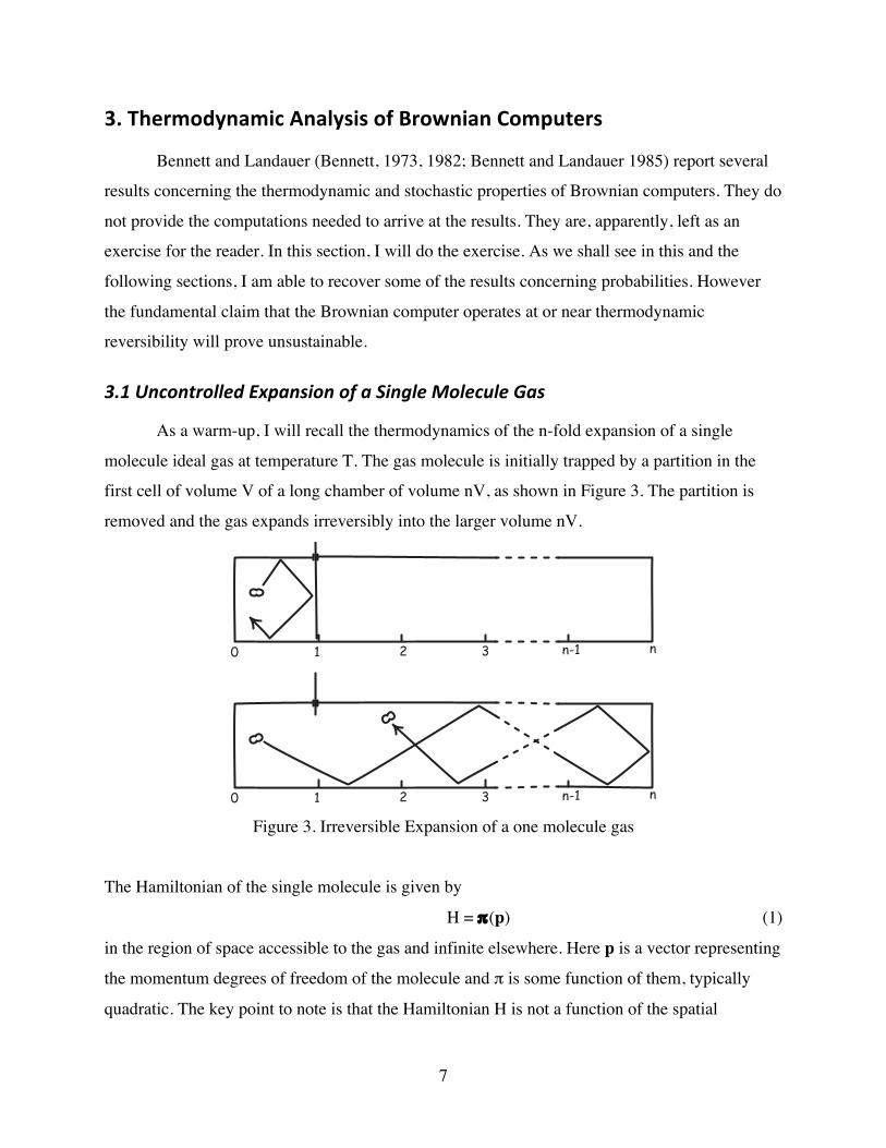
As a warm-up, I will recall the thermodynamics of the n-fold expansion of a single

molecule ideal gas at temperature T. The gas molecule is initially trapped by a partition in the

first cell of volume V of a long chamber of volume nV, as shown in Figure 3. The partition is

removed and the gas expands irreversibly into the larger volume nV.

0 1 2 3 n-1 n

0 1 2 3 n-1 n Figure 3. Irreversible Expansion of a one molecule gas

The Hamiltonian of the single molecule is given by

H = π(p) (1)

in the region of space accessible to the gas and infinite elsewhere. Here p is a vector representing

the momentum degrees of freedom of the molecule and π is some function of them, typically

quadratic. The key point to note is that the Hamiltonian H is not a function of the spatial

8

coordinates x = (x, y, z) of the molecule. This independence drives the results that follow. We

assume that the x coordinate is aligned with the long axis of the chamber and that it has a cross-

sectional area A.

At thermal equilibrium, the molecule’s position is Boltzmann distributed probabilistically

over its phase space as

p(x,p) = exp(-H/kT)/Z(λ) (2)

where we assume the molecule is confined to a region x=0 to x=λ of the chamber. Using V=A.1,

the partition function Z(λ) associated with the molecule confined to the region x=0 to x=λ is

€

Z(λ) =all p∫ exp(−H / kT )Adxdp =Vλ exp(−π (p) / kT )

all p∫x=0

λ

∫ dp (3)

The associated canonical thermodynamic entropy is

€

S(λ) =∂∂T(kT lnZ(λ)) = k ln(Vλ)+ Sp (T ) (4)

The contribution of the momentum degrees of freedom is absorbed into a constant Sp(T) that will

not figure in the subsequent calculations. The independence of the Hamiltonian (1) from the

position coordinates leads to the characteristic logarithmic volume dependence of the canonical

entropy (4), that is, that S(λ) varies as k ln (Vλ).

It follows that the thermodynamically irreversible n-fold increase in volume of the one

molecule gas from λ=1 to λ=n is associated with an entropy change

ΔSgas = k ln (Vn) – k ln V = k ln n (5)

During the expansion, the mean energy of the gas remains constant and, since it does no work,

no net heat is exchanged with the environment. Since the environment is unchanged, we have for

its thermodynamic entropy change

ΔSenv = 0 (6)

Thus the total entropy change is

ΔStot = ΔSgas + ΔSenv = k ln n (7)

Since the internal energy E is remains the same, it follows from (5) that the change in free energy

F = E –TS of the gas is

ΔFgas = - kT ln n (8)

We recover the same result from (3) and the canonical expression F = -kT ln Z.

9

The essential point for what follows is that this expansion is driven entirely by entropic

forces. There is no energy gradient driving it; the internal energy E of the gas is the same at the

start of the expansion, when it is confined to volume V, as at the end, when it occupies a volume

nV.

More generally, this sort of process is driven by an imbalance of a generalized

thermodynamic force. For isothermal processes whose stages are parameterized by λ, the

appropriate generalized force is

X = - (∂F/∂λ) (9)

If we parameterize the states of the isothermally expanding one molecule gas by the volume

V(λ) = Vλ, occupied at stage λ, then F(λ)= -kT ln V(λ) and the generalized force adopts the

familiar form of the pressure of a single-molecule ideal gas:

€

X =T ∂k lnV (λ)∂V (λ)

=kTV (λ)

(10)

3.2  Brownian  Motion  

One of the papers of Einstein’s annus mirabilis of 1905 gives his analysis of Brownian

motion (Einstein, 1905). In the paper he noted that the thermal motions of small particles

suspended in a liquid would be observable under a microscope and he conjectured that their

motions were the same as those observed in pollen grains by the botanist Brown. Einstein’s goal

was to give an account of these thermal motions within the molecular-kinetic theory of heat and

thereby finally to establish it as the correct account of thermal processes.2

His starting point was to propose the astonishing idea that, from the perspective of the

molecular-kinetic theory, individual molecules and microscopically visible particles can be

treated by the same analysis and will give the same results. To reflect this astonishing idea, the

analysis just given above of the statistical physics of a single molecule, has been written in such

a way that it can be applied without change to a microscopically visible particle, such as a pollen

grain. The controlling fact is that the Hamiltonian for a microscopically visible particle can be

written as (1), for the energy of the particle will be independent of its position in the suspending

liquid. The particular expression π(p), which gives the dependence of the Hamiltonian on the

2 For an account of Einstein analysis, see Norton (2006, Section 3).

10

momentum degrees of freedom, will be different. For the particle is, to first approximation,

moving through a resisting, viscous medium. However this difference will not affect the results

derived above.

First, we will be able to conclude that a single Brownian particle will exert a pressure

conforming to the ideal gas law, as shown in (10). What this means is that the collisions of the

Brownian particle with the walls confining it to some volume V will lead to a mean pressure

equal to kT/V on the walls. Einstein considered the case of the confining walls as a semi-

permeable membrane that allows the liquid but not the particle to pass. Then the pressure is

appropriately characterized as an osmotic pressure.

Second, the volume dependence of the thermodynamic entropy of the Brownian particle

will conform to (4), so that an n-fold expansion of the volume accessible to the particle will be

associated with an increase of thermodynamic entropy of ΔS = k ln n as shown in (5). By the

same reasoning as in the case of the one molecule gas, the increase in total entropy is also ΔStot =

k ln n as given by (7).

In direct analogy with the irreversible expansion described above for a single molecule

gas, we can form a liquid filled chamber of volume nV with the Brownian particle trapped by a

partition in the leftmost volume V, as shown in Figure 4. The particle exerts a pressure on the

partition of kT/V. When the partition is removed, the unopposed pressure will lead to a

thermodynamically irreversible expansion of the one Brownian particle gas into the full

chamber. The uncontrolled expansion from volume V to nV is associated with the creation of k

ln n of thermodynamic entropy.

0 1 2 3 n-1 n

0 1 2 3 n-1 n Figure 4. Irreversible Expansion of a one Brownian particle gas

11

Thermodynamically, the expansion of the one molecule gas and the one Brownian

particle gas are the same. The two Figures 3 and 4, however, suggest the great dynamical

differences. Ordinary gas molecules at normal temperatures move quickly, typically at many

hundreds of meters per second. The motion of the one molecule is unimpeded by any other

molecules, so it moves freely between the collisions with the walls. Brownian particles have the

same mean thermal energy of kT/2 per degree of freedom. But since they are much more

massive than molecules, their motion is correspondingly slower. More importantly, they undergo

very many collisions: the jiggling motion of a pollen grain visible under a microscope is the

resultant of enormously many collisions with individual water molecules in each second.

This means that the expansion of the one Brownian particle gas is very much slower than

that of the one molecule gas. When we observe the Brownian particle under the microscope, we

are watching it for the briefest moment of time if we set our time scales according to how long

the particle will take to explore the volume accessible to it. If we were to watch it for an

extended time, we would see that the particle has adopted a new equilibrium state in which it

explores the full volume nV, just as the expanded one molecule gas explores the same volume

nV.

These differences of time scales between the one molecule gas and the one Brownian

particle gas are irrelevant, however, to the thermal equilibrium states. Both gases start out in an

equilibrium state confined to a volume V; they undergo an uncontrolled, n-fold expansion to a

new equilibrium state confined to volume nV; and their thermodynamic entropies each increase

by k ln n.

These remarks draw on the analysis of the earlier parts of Einstein’s (1905) paper. In

sections 3 and later, he took up another aspect of Brownian motion that will not arise in the

otherwise analogous physics of Brownian computers. Einstein modeled the Brownian particles as

spheres and the surrounding water as a viscous fluid. (There is no analog of the fluid in the

Brownian computer.) Einstein then modeled the diffusion of Brownian particles through the

liquid as governed by the balance of two forces: the driving force of osmotic pressure in a

gradient of particles and the opposing viscous forces as the particles move. What matters for our

purposes is that Einstein eventually arrived at a result in the new theory of stochastic processes

being created by his paper that is more general that the particular case he analyzed.

12

It is a result concerning particles, such as Brownian particles, that are animated in a

random walk. Their positions spread through space according to a Gaussian distribution whose

spatial variance is proportional to time. It follows that the average (absolute) distance d(t)

covered in some time t is proportional to

€

t . This means that we cannot speak meaningfully of

the average speed over time of the Brownian particle, for that average speed

d(t)/t is proportional to 1/

€

t → 0 as t→∞ (11)

That is, if one tries to estimate average speed by forming the familiar ratio “distance/time,” that

ratio can be made arbitrarily small by allowing time to become arbitrarily large. Einstein (1907,

p. 42) remarks that the “…speed thus provided corresponds to no objective property of the

motion investigated…”

3.3  The  Undriven  Brownian  Computer  without  Trap  

A Brownian computer behaves thermodynamically like a one molecule gas or a one

Brownian particle gas expanding irreversibly into its configuration space. Here I will develop the

simplest case of the undriven Brownian computer without a trap. This is the case that is closest to

the irreversible expansion of a one molecule/Brownian particle gas. While it does not terminate

the computation usefully, it sets the minimum thermodynamic entropy creation for all Brownian

computers. Later we will add extra processes, such as a slight energy gradient to drive the

computation faster, or an energy trap to terminate it. Each of these additions will create further

thermodynamic entropy.

In this simplest case, the Brownian computer explores a one-dimensional labyrinthine

channel in its phase space. All spatial configurations in the channel are assumed to have the same

energy; there is no energy gradient pressing the system in one or other direction. As a result, the

Hamiltonian of the Brownian computer is of the form (1), where we have the controlling fact that

it depends only on the momentum degrees of freedom. The analysis proceeds as before.

We divide the very high dimensional configuration space of the computer into n stages.

Precisely how the division is effected will depend upon the details of the implementation. One

stage may correspond to all configurations in which the Turing machine reader head is

interacting directly with one particular tape cell. For simplicity, we will assume that each stage

occupies the same volume V in configuration space. Progress through the channel is

parametrized by λ, which counts off the stages passed.

13

To operate the computer, its state is localized initially in the volume of phase space

corresponding to the first stage, λ=0 to λ=1. The device is then unlocked—the thermodynamic

equivalent of removing the partition in the gas case—and the computer undertakes a random

walk through the accessible channel in its phase space. As with the one molecule gas, changes in

the momentum degrees of freedom play no role in the expansion. The computer settles down into

a new equilibrium state in which it explores the full volume nV of the channel of its

configuration space. The expansion is driven by an unopposed generalized force X given by (9),

and with a volume dependence in configuration space of the single-molecule ideal gas law (10)

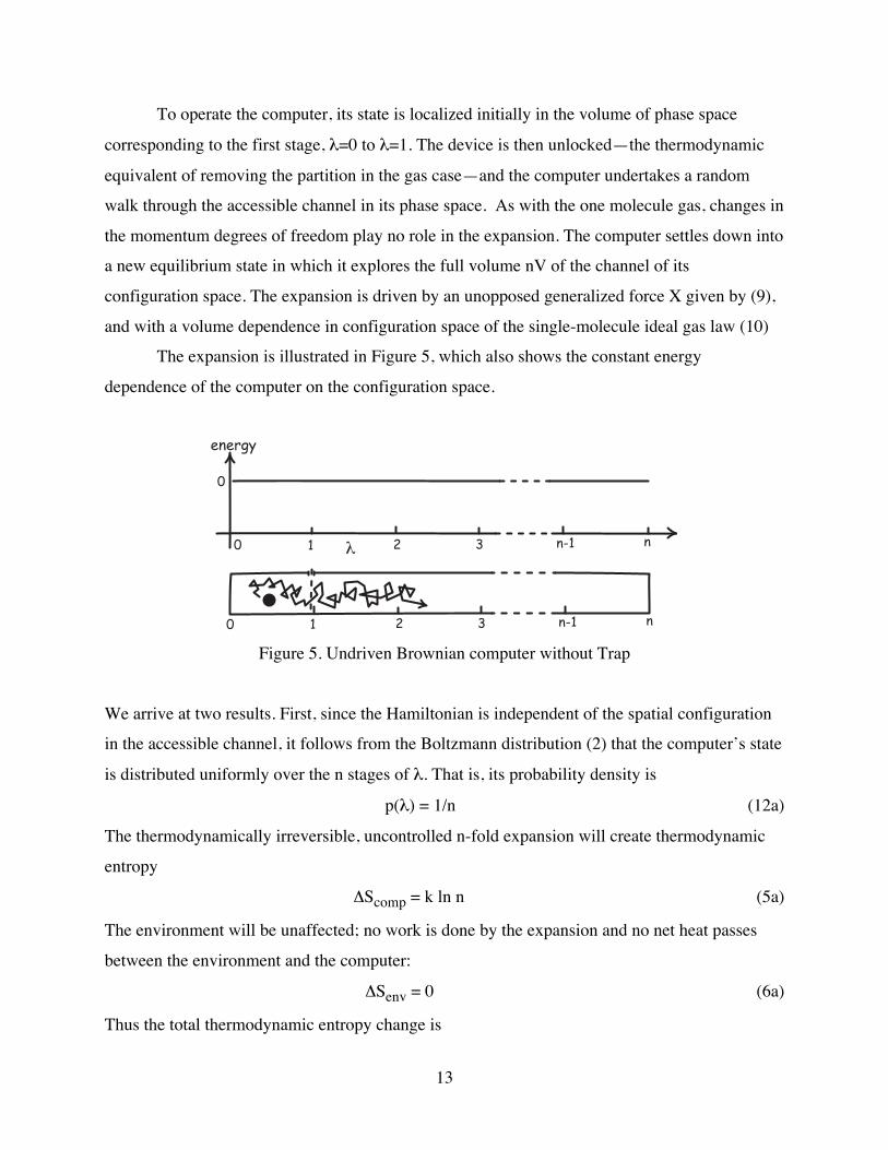
The expansion is illustrated in Figure 5, which also shows the constant energy

dependence of the computer on the configuration space.

0

0

0

1 2 3 n-1 n

1 2 3 n-1 n!

energy

Figure 5. Undriven Brownian computer without Trap

We arrive at two results. First, since the Hamiltonian is independent of the spatial configuration

in the accessible channel, it follows from the Boltzmann distribution (2) that the computer’s state

is distributed uniformly over the n stages of λ. That is, its probability density is

p(λ) = 1/n (12a)

The thermodynamically irreversible, uncontrolled n-fold expansion will create thermodynamic

entropy

ΔScomp = k ln n (5a)

The environment will be unaffected; no work is done by the expansion and no net heat passes

between the environment and the computer:

ΔSenv = 0 (6a)

Thus the total thermodynamic entropy change is

14

ΔStot = ΔScomp + ΔSenv = k ln n (7a)

This is the minimum thermodynamic entropy creation associated with the operation of the

Brownian computer. Embellished versions below add processes that create more thermodynamic

entropy.

As before, the free energy change is

ΔFcomp = - kT ln n (8a)

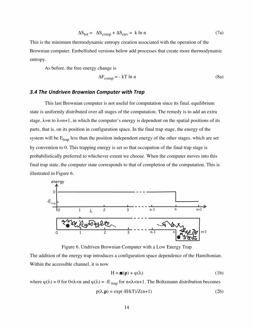
3.4  The  Undriven  Brownian  Computer  with  Trap  

This last Brownian computer is not useful for computation since its final, equilibrium

state is uniformly distributed over all stages of the computation. The remedy is to add an extra

stage, λ=n to λ=n+1, in which the computer’s energy is dependent on the spatial positions of its

parts, that is, on its position in configuration space. In the final trap stage, the energy of the

system will be Etrap less than the position independent energy of the other stages, which are set

by convention to 0. This trapping energy is set so that occupation of the final trap stage is

probabilistically preferred to whichever extent we choose. When the computer moves into this

final trap state, the computer state corresponds to that of completion of the computation. This is

illustrated in Figure 6.

0

0

0

1 2 3 n-1 n n+1

n+11 2 3 n-1 n!

energy

-Etrap

Figure 6. Undriven Brownian Computer with a Low Energy Trap

The addition of the energy trap introduces a configuration space dependence of the Hamiltonian.

Within the accessible channel, it is now

H = π(p) + ϕ(λ) (1b)

where ϕ(λ) = 0 for 0<λ<n and ϕ(λ) = -E trap for n<λ<n+1. The Boltzmann distribution becomes

p(λ,p) = exp(-H/kT)/Z(n+1) (2b)

15

where the partition function is

€

Z(n+1) = exp(−H / kT )dxdp = exp(−π (p)all p∫∫ / kT )dp ⋅ exp(−ϕ(λ)

λ=0

n+1∫ / kT )Vdλ

€

= M ⋅V ⋅ (n+ exp(Etrap / kT )) (3b)

using the fact that the volume element of configuration space dx = Vdλ and writing the

contribution from the momentum degrees of freedom as

€

M = exp(−π (p)all p∫ / kT )dp . Since the

momentum degrees of freedom are uninteresting, we integrate them out and recover the

probability densities

€

p(λ) =1

n+ exp(Etrap / kT ) for 0<λ<n

€

p(λ) =exp(Etrap / kT )

n+ exp(Etrap / kT ) for n<λ<n+1 (12b)

It follows that the probability P that the computer is in the trap state n<λ<n+1 is

P = 1/(1 + n.exp(-Etrap/kT)) OP = exp(Etrap/kT)/n

where OP = P/(1-P) is the odds of the computer being in the final trap state. Inverting this last

expression enables us to determine how large the trapping energy Etrap should be for any

nominated P or OP:

Etrap = kT(ln n + ln OP) = kT ln n + kT ln (P/(1-P)) (13b)

We compute the thermodynamic entropy of the expanded equilibrium state as

€

S(n+1) =∂∂T(kT lnZ(n+1)) =

∂∂T(kT lnM )+ ∂

∂T(kT lnV )+ ∂

∂T(kT ln(n+ exp(Etrap / kT ))

€

= Sp(T )+ k lnV + k ln(n+ exp(Etrap / kT ))−P ⋅Etrap /T (4b)

The first term Sp(T) represents the contribution of the momentum degrees of freedom and is

independent of stage of computation achieved. Hence, as before, it need not be evaluated more

specifically.

The thermodynamic entropy of the initial state is S(1) = Sp(T) + k ln V as before.

Therefore, the increase in thermodynamic entropy in the course of the thermodynamically

irreversible expansion and trapping of the computer state is

ΔScomp = k ln (n + exp(Etrap/kT)) – P. Etrap/T (5b)

In the course of the thermodynamically irreversible expansion, when the system falls into the

final energy trap, it will release energy Etrap as heat to the environment. More carefully, on

16

average it will release energy P. Etrap since the computer state will only be in the trap with high

probability P. This will increase the thermodynamic entropy of the environment by3

ΔSenv = P. Etrap/T (6b)

Thus the total thermodynamic entropy change is

ΔStot = ΔScomp + ΔSenv = k ln (n + exp(Etrap/kT))

= k ln n + k ln (1+ OP) (7b)

Hence the effect of adding the trap is to increase the net creation of thermodynamic entropy over

that of the untrapped system (7a) by the second term k ln (1+ OP) = k ln (1/(1-P)). The added

term will be larger according to how much we would like the trap state to be favored, that is,

how large we set the odds OP.

Rearranging (5b), we find that change in free energy F=E-TS is

ΔFcomp = - kT ln n - kT ln (1+ OP) (8b)

We recover the same result from (3b) and the canonical expression F = -kT ln Z.

3.5  The  Energy  Driven  Brownian  Computer  without  Trap  

This last case of the undriven but trapped Brownian computer is sufficient to operate a

Brownian computer. Bennett (1973, p. 531; 1982, p. 921), however, includes the complication

of a slight energy gradient in the course of the computation, in order to speed up the

computation. We can understand the thermodynamic import of this augmentation by considering

the simpler case of an energy gradient driven computer, without the energy trap.

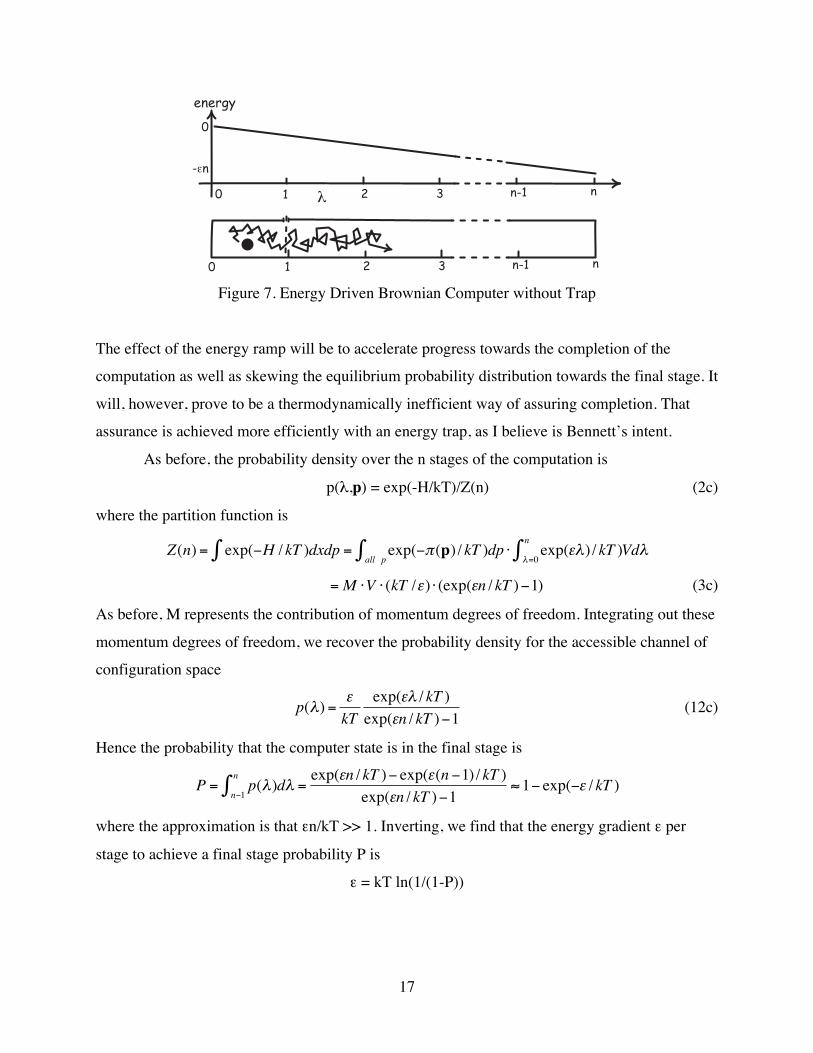
The energy gradient is included by assuming that there is linear spatial dependence of the

energy of the system on the parameter λ that tracks progress through the accessible channel in

the phase space. That is, we assume an energy ramp of ε per stage. The Hamiltonian becomes:

H = π(p) - ελ (1c)

This is illustrated in Figure 7.

3 While the process is not thermodynamically reversible, we recover the same thermodynamic

entropy change for the environment by imagining another thermodynamically reversible process

in which heat energy P. Etrap is passed to the environment.

17

0

0

0

-!n

1 2 3 n-1 n

1 2 3 n-1 n"

energy

Figure 7. Energy Driven Brownian Computer without Trap

The effect of the energy ramp will be to accelerate progress towards the completion of the

computation as well as skewing the equilibrium probability distribution towards the final stage. It

will, however, prove to be a thermodynamically inefficient way of assuring completion. That

assurance is achieved more efficiently with an energy trap, as I believe is Bennett’s intent.

As before, the probability density over the n stages of the computation is

p(λ,p) = exp(-H/kT)/Z(n) (2c)

where the partition function is

€

Z(n) = exp(−H / kT )dxdp = exp(−π (p)all p∫∫ / kT )dp ⋅ exp(ελ)

λ=0

n∫ / kT )Vdλ

€

= M ⋅V ⋅ (kT /ε) ⋅ (exp(εn / kT )−1) (3c)

As before, M represents the contribution of momentum degrees of freedom. Integrating out these

momentum degrees of freedom, we recover the probability density for the accessible channel of

configuration space

€

p(λ) =εkT

exp(ελ / kT )exp(εn / kT )−1

(12c)

Hence the probability that the computer state is in the final stage is

€

P = p(λ)dλn−1

n∫ =

exp(εn / kT )− exp(ε(n −1) / kT )exp(εn / kT )−1

≈ 1− exp(−ε / kT )

where the approximation is that εn/kT >> 1. Inverting, we find that the energy gradient ε per

stage to achieve a final stage probability P is

ε = kT ln(1/(1-P))

18

For desirable values of P that are close to unity, this last formula shows that a steep energy

gradient is needed. For a P = 0.99, we would require ε = kT ln(100) = 4.6 kT. Finally, If we

assume in addition that ε << kT, this probability reduces to

P = 1 - exp(-ε/kT) ≈ ε/kT,

This conforms with Bennett’s (1973, p.51) remark that:

…if the driving force ε is less than kT, any Brownian computer will at equilibrium

spend most of its time in the last few predecessors of the final state, spending about

ε/kT of its time in the final state itself

Before computing the thermodynamic entropy change, it will be convenient to compute

the mean energy of the initial state E(1) and the final state E(n) associated with the configuration

space degrees of freedom. We have for the mean energy that

€

E(n) = kT 2 ∂∂TlnZ(n)

€

= kT 2 ∂∂TlnM + kT 2 ∂

∂Tln(kT /ε)+ kT 2 ∂

∂Tln(exp(εn / kT )−1)

€

= Ep(T )+ kT −εn

1− exp(−εn / kT )

where Ep(T) represents the contribution of the momentum degrees of freedom and is independent

of stage of computation achieved. Setting n=1, we find

€

E(1) = Ep (T )+ kT −ε

1− exp(−ε / kT )

We now compute the thermodynamic entropy of the final equilibrium state as4

€

S(n) =∂∂T(kT lnZ(n))

€

=∂∂T(kT lnM )+ ∂

∂T(kT lnV )+ ∂

∂T(kT ln(kT /ε))+ ∂

∂T(kT ln(exp(εn / kT )−1))

€

= Sp(T )−Ep (T ) /T + k lnV + k ln(kT /ε)+ k ln(exp(εn / kT )−1)+E(n) /T

€

= k lnV + k ln(kT /ε)+ k ln(exp(εn / kT )−1)+E(n) /T (4c)

4 The expression is simplified using Sp(T) = Ep(T)/T. This follows from considering the

momentum degrees of freedom contribution to both entropy and energy during a

thermodynamically reversible heating from T=0.

19

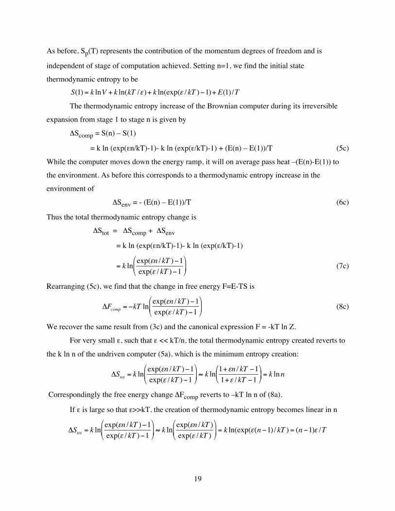
As before, Sp(T) represents the contribution of the momentum degrees of freedom and is

independent of stage of computation achieved. Setting n=1, we find the initial state

thermodynamic entropy to be

€

S(1) = k lnV + k ln(kT /ε)+ k ln(exp(ε / kT )−1)+E(1) /T

The thermodynamic entropy increase of the Brownian computer during its irreversible

expansion from stage 1 to stage n is given by

ΔScomp = S(n) – S(1)

= k ln (exp(εn/kT)-1)- k ln (exp(ε/kT)-1) + (E(n) – E(1))/T (5c)

While the computer moves down the energy ramp, it will on average pass heat –(E(n)-E(1)) to

the environment. As before this corresponds to a thermodynamic entropy increase in the

environment of

ΔSenv = - (E(n) – E(1))/T (6c)

Thus the total thermodynamic entropy change is

ΔStot = ΔScomp + ΔSenv

= k ln (exp(εn/kT)-1)- k ln (exp(ε/kT)-1)

€

= k ln exp(εn / kT )−1exp(ε / kT )−1

⎛

⎝ ⎜

⎞

⎠ ⎟ (7c)

Rearranging (5c), we find that the change in free energy F=E-TS is

€

ΔFcomp = −kT ln exp(εn / kT )−1exp(ε / kT )−1

⎛

⎝ ⎜

⎞

⎠ ⎟ (8c)

We recover the same result from (3c) and the canonical expression F = -kT ln Z.

For very small ε, such that ε << kT/n, the total thermodynamic entropy created reverts to

the k ln n of the undriven computer (5a), which is the minimum entropy creation:

€

ΔStot = k ln exp(εn / kT )−1exp(ε / kT )−1

⎛

⎝ ⎜

⎞

⎠ ⎟ ≈ k ln

1+εn / kT −11+ε / kT −1

⎛

⎝ ⎜

⎞

⎠ ⎟ = k lnn

Correspondingly the free energy change ΔFcomp reverts to –kT ln n of (8a).

If ε is large so that ε>>kT, the creation of thermodynamic entropy becomes linear in n

€

ΔStot = k ln exp(εn / kT )−1exp(ε / kT )−1

⎛

⎝ ⎜

⎞

⎠ ⎟ ≈ k ln

exp(εn / kT )exp(ε / kT )

⎛

⎝ ⎜

⎞

⎠ ⎟ = k ln(exp(ε(n −1) / kT ) = (n −1)ε /T

20

which grows with n much faster than the logarithm in k ln n. Since large values of ε would be

needed to drive the system into its final stage with high probability, this method of assuring

termination of the computation is thermodynamically costly.

3.6  The  Energy  Driven  Brownian  Computer  with  Trap  

Finally, I will provide an abbreviated account of the case of a Brownian computer that is

both driven by an energy gradient and brought to completion with an energy trap. Its

Hamiltonian is a combination of the two earlier cases

H = π(p) + ϕ(λ) (1d)

where

ϕ(λ) = - ελ for 0<λ<n

= - εn -E trap for n<λ<n+1.

It is illustrated in Figure 8.

0

0

0

1 2 3 n-1 n n+1

n+11 2 3 n-1 n!

energy

-"n-Etrap

-"n

Figure 8. Energy Driven Brownian Computer with Energy Trap

Since this case incorporates both dissipative processes added in the last two cases, in operation it

will create more thermodynamic entropy than any case seen so far, that is, in excess of k ln n, so

I will not compute the thermodynamic entropy created.

If P is the probability that the fully expanded system is in the trap, we can compute the

odds ratio OP = P/(1-P) by taking the ratio of the partition functions for the two regions of phase

space: Z(n) for the first n stages and Z(trap) for the final trap state n<λ<n+1. From (3c) and (3b)

we have

€

Z(n) = M ⋅V ⋅ (kT /ε) ⋅ (exp(εn / kT )−1)

21

€

Z(trap) = M ⋅V ⋅ exp((εn+Etrap ) / kT )

We have for the odds ratio

€

Op =P1−P

=Z(trap)Z(n)

=exp((εn+Etrap ) / kT )

(kT /ε) ⋅ (exp(εn / kT )−1)=εkT

⋅exp(Etrap / kT )1− exp(−εn / kT )

We can invert this last expression to yield

Etrap = kT ln (kT/ε) + kT ln (1- exp(-εn/kT)) + kT ln OP (13d)

It reverts to the corresponding expression (13b) for the undriven Brownian computer when we

assume that εn/kT << 1, for then

kT ln (kT/ε) + kT ln (1- exp(-εn/kT)) ≈ kT ln (kT/ε) + kT ln (εn/kT) = kT ln n

If instead we assume more realistically that εn/kT >> 1, so that exp(-εn/kT) ≈ 0, we recover

Etrap = kT ln (kT/ε) + kT ln OP = kT ln (OP kT/ε)

This seems to be the result to which Bennett (1982, p. 921) refers when he writes:

However the final state occupation probability can be made arbitrarily large,

independent of the number of steps in the computation, by dissipating a little extra

energy during the final step, a “latching energy” of kT ln (kT/ε) + kT ln (1/η)

sufficing to raise the equilibrium final state occupation probability to 1- η.

The two results match up close enough if we set P=1- η and approximate OP ≈ 1/(1-P)

when P is very close to unity. However the result does not conform quite as well with

Bennett’s (1973, p. 531) remark that:

If all steps had equal dissipation, ε<kT, the final state occupation

probability would be only about ε/kT. By dissipating an extra

kT ln (3 kT/ε) of energy during the last step, this probability is

increased to about 95%.

A final stage probability of P = 0.95 corresponds to an odds ratio of OP = 20, so that the

extra energy dissipated should be kT ln (20 kT/ε). Compatibility would be restored if we

assume a missing “+” in Bennett’s formula, for ln 20 = 3, so that

kT ln (20 kT/ε) = kT ln 20 + kT ln (kT/ε) = kT (3 + ln (kT/ε))

22

4  Thermodynamic  Reversibility  is  Mistakenly  Attributed  to  Brownian  

Computers  

The results of the last section can be summarized as follows. An n stage computation on a

Brownian computer is a thermodynamically irreversible process that creates a minimum of k ln n

of thermodynamic entropy (see equation (7a)). Additional thermodynamic entropy of k ln (1+

OP) is created to complete the computation by trapping the computer state in a final energy trap

with probability odds OP (see equation (7b)). If we accelerate the computation by adding an

energy gradient of ε per stage, we introduce further creation of thermodynamic entropy

according to equation (7c). For a larger gradient, the thermodynamic entropy created grows

linearly with the number of stages.

While it is thermodynamically irreversible, a Brownian computer is routinely misreported

as operating thermodynamically reversibly. Bennett (1984) writes:

A Brownian computer is reversible in the same sense as a Carnot engine: Both

mechanisms function in the presence of thermal noise, both achieve zero

dissipation in the limit of zero speed, and both are, in accordance with

thermodynamic convention, presumed to be absolutely stable against structural

decay (e.g., thermal annealing of a piston into a more rounded shape), despite

their being non-equilibrium configurations of matter.

This misreporting is especially awkward since the case of the Brownian computer is offered as

the proof of a core doctrine in the recent thermodynamics of computation: that logically

reversible operations can be computed by thermodynamically reversible processes. Bennett

(1988, pp. 329-31) reports that the “proof of the thermodynamic reversibility of computation [of

logically reversible operations]” arose through the investigation into the biochemistry of DNA

and RNA that culminated in the notion of the Brownian computer. Bennett (2003, p. 531) reports

that the objection against thermodynamically reversible computation of logically reversible

operations “has largely been overcome by explicit models.” He then cites the non-

thermodynamic, hard sphere model of Fredkin and Toffoli; and “at a per-step cost tending to

zero in the limit of slow operation (so-called Brownian computers discussed at length in my

review article; [(Bennett, 1982)]).”

23

5.  Thermodynamically  Reversible  Processes  

Evidently, thermodynamically reversible processes can be hard to identify correctly. The

above misidentification remains unchallenged in the literature. Hence it will be useful to review

here just what constitutes thermodynamic reversibility and how it can be misidentified.

5.1  What  They  Are  

The key notion in a thermodynamically reversible process is that all thermodynamic

driving forces are in perfect balance. This traditional conception is found in the old text-books.

Poynting and Thomson (1906, p. 264) give the “conditions for reversible working” that

“indefinitely small changes in the external conditions shall reverse the order of change.” They

list these conditions as: bodies exchanging heat “never differ sensibly” in temperature; and that

the “pressure exerted by the working substance shall be sensibly equal to the load.” It follows

that “exactly reversible processes are ideal, in that exact reversibility requires exact equilibrium

with surroundings, that is, requires a stationary condition.” This means that nothing changes, so

there is no process. They then offer the familiar escape:5

…we can approximate as closely as we like to the conditions of reversibility, by

making the conditions as nearly as we like [to] those required, and lengthening

out the time of change.

Planck (1903, §§71-73) gives an essentially similar account. He writes of pressures that differ

“just a trifle,” “infinitesimal differences of temperature” and “infinitely slow” progress. The

process consists of “a succession of states of equilibrium.” More fully:

If a process consists of a succession of states of equilibrium with the exception of

very small changes, then evidently a suitable change, quite as small, is sufficient

to reverse the process. This small change will vanish when we pass over to the

limiting case of the infinitely slow process…

5 It is quite delicate matter to explain the cogency of the notion of a thermodynamically

reversible process when proper realization of the process entails that nothing changes, so no

process occurs. For my attempt see Norton (forthcoming b).

24

We need only add to these classic accounts that generalized thermodynamic forces, such as those

derived from (9) and which generalize the notion of pressure, must also be in balance.

When a Brownian particle is released into a liquid, its resulting exploration of the

accessible volume is driven, thermodynamically speaking, by an unbalanced osmotic pressure, as

Einstein argued in his celebrated analysis of 1905. Hence it is a thermodynamically irreversible

expansion. Correspondingly, when a Brownian computer is set into its initial state and then

allowed to explore the accessible computational space, the exploration is a thermodynamically

irreversible process.

5.2  How  We  Might  Misidentify  Them    

There are many ways we may come to misidentify a thermodynamically irreversible

process as thermodynamically reversible.

Infinite slowness is not sufficient to identify thermodynamic reversibility.

While thermodynamically reversible processes are infinitely slow, the converse need not hold.

Sommerfeld (1962, p. 17) gives the simple example of an electrically charged capacitor that can

be discharged arbitrarily slowly through an arbitrarily high resistance. While the process can be

slowed indefinitely, it is a thermodynamically irreversible conversion of the electrical energy of

the capacitor into heat. The driving voltage is not balanced by an opposing force. A simpler

example is the venting of a gas at high pressure into a vacuum through a tiny pinhole. The

process can be slowed arbitrarily, but it is not thermodynamically reversible since the gas

pressure is unopposed.

Reversibility of the microscopic or molecular dynamics not sufficient to assure

thermodynamic reversibility.

One cannot discern thermodynamic reversibility by affirming the reversibility of the individual

processes that comprise the larger process at the microscopic or molecular level. They may be

reversible, in the sense that they can go either way, while the overall process is itself

thermodynamically irreversible. As a general matter, any thermodynamically irreversible process

25

may be reversed by a vastly improbable fluctuation. That possibility depends upon the

microscopic reversibility of the underlying processes.6

A pertinent example is the thermodynamically irreversible expansion of a one molecule

gas. Its momentary, microscopic behavior is reversible. To see this, consider a one molecule gas

suddenly released into a large chamber filled with fixed, oddly shaped obstacles. If we simply

attend to the molecule’s motion over a brief period of time, while it undergoes one or two

collisions, we would see mechanically reversible motions, as illustrated in Figure 9.

0 1 2 3 n-1 n

0 1 2 3 n-1 n Figure 9. Microscopic Reversibility of a Thermodynamically Irreversible Expansion

However that would mislead us. We need to attend to the initial low entropy state of confinement

of the one molecule gas; and its final high entropy state in which it explores the larger volume

freely in order to recognize the thermodynamically irreversible character of the expansion. 6 For isothermal, isobaric chemical reactions, the relevant generalized force is the chemical

potential µA = (∂GA/∂nA)T,P, where G = E + PV – TS is the Gibbs free energy of reagent A and

nA the number of moles of A. In dilute solutions, µA = µA0 + RT ln [A] for R the ideal gas

constant, µA0 the chemical potential at reference conditions and [A] the molar concentration.

While each chemical reaction is reversible at the molecular level, the term RT ln [A] contributes

an entropic force, so that a chemical reaction will be thermodynamically irreversible if the

concentrations of the reagents and products are not constantly adjusted to keep them at

equilibrium levels.

26

Precisely the same must be said for both Brownian motion and a Brownian computer.

They are both initialized in a state of low thermodynamic entropy; and then expand in a

thermodynamically irreversible process to explore a larger space. At any moment, however, their

motions will be mechanically reversible. We would be unable to tell whether we are observing

their development forward in time or a movie of that development run in reverse. To separate the

two, we would need to observe long enough to see whether the time evolution carries the system

to explore the larger accessible space or whether it carries it back to its initial state of

confinement.

Bennett (1982, p, 912) reports that a Brownian computer “is about as likely to proceed

backward along the computational path, undoing the most recent transition, as to proceed

forward.” Similarly Bennett and Landauer (1985, p. 54) report for the Brownian computer that

“[i]t is nearly as likely to proceed backward along the computational path, undoing the most

recent transition, as it is to proceed forward.”7

This sort of reversibility is insufficient to establish thermodynamic reversibility.

Tracking internal energy instead of thermodynamic entropy is insufficient to identify

thermodynamic reversibility.

A thermodynamically reversible process is one in which the total thermodynamic entropy Stot =

Ssys + Senv remains constant, where Ssys is the thermodynamic entropy of the system and Senv

that of the environment. Thermodynamically reversible processes must be identified by tracking

this entropy. They cannot be identified by tracking internal energy changes.

What confounds matters is that we often track thermodynamic reversibility by means of

quantities that carry the label “energy,” such as free energy F = E-TS. These energies are useable

this way in so far as they are really measures of thermodynamic entropy adapted to special

conditions. For example, Brownian computers implement isothermal processes while in thermal

contact with an environment with which they exchange no work. Hence, if we have a

thermodynamic process parameterized by λ so that d = d/dλ, then the constant entropy condition

of thermodynamic reversibility for a computer “comp” in a thermal environment “env” is

0 = dStot = dScomp + dSenv = dScomp –dEcomp/T = - dFcomp/T. 7 I believe the “nearly” refers to the small external force they add corresponding to the energy

ramp of Section 3.5 above.

27

It corresponds to constancy of the free energy Fcomp of the computer.

Tracking internal energies gives the wrong result for Brownian computers. The

thermodynamically irreversible n stage expansion of the Brownian computer is a constant energy

process. The final energy trap could be replaced by a trap stage with a large volume Vtrap =

NtrapV of accessible configuration space. Then the final trapping can also be effected without

any change of internal energy. The odds for the computer state being in the trap are OP = P/(1-P)

= Ntrap/n. Using (7a), the total thermodynamic entropy created is

ΔStot = ΔScomp + ΔSenv = k ln (n + Ntrap)

= k ln n + k ln (1+ Ntrap/n) = k ln n + k ln (1+ OP)

which agrees with the thermodynamic entropy creation of the energy trap (7b).

Bennett (1973, p. 531) introduced a small energy gradient in order to bring some

“positive drift velocity” into Brownian computation. As we saw in Section 3.2 and equation (11),

without it, no average speed can be assigned to Brownian motion. However it is also unnecessary

for completion of the computational processes. They proceed as does any diffusion process, with

progress increasing with the square root of time. That means the computation will take longer to

complete. Since temporal efficiency is not the issue, there seems no point in including a

superfluous source of thermodynamic irreversibility.

In assessing the thermodynamic efficiency of the Brownian computation of logically

reversible functions, Bennett and Landauer do not track thermodynamic entropy. Rather they

track the wrong quantity, energy. Bennett writes of energy “dissipated,” both as the energy ε per

step and in the trap energy or “latching” energy Etrap. See Bennett (1973, p. 531; 1982, p. 915,

921). Bennett and Landauer (1985, pp. 54-56) write of energy “expended” or “dissipated”:

A small force, provided externally, drives the computation forward. This force

can again be as small as we wish, and there is no minimum amount of energy that

must be expended in order to run a Brownian clockwork Turing machine.

and

The machine can be made to dissipate as small an amount of energy as the user

wishes, simply by employing a force of the correct weakness.

If the energy ε per stage is made arbitrarily small, the change of internal energy E of the

Brownian computer will also become arbitrarily small. However it would be an elementary error

28

to confuse that with the operation of the computer becoming thermodynamically reversible, so

that no net thermodynamic entropy is created; or to confuse it with the change in free energy

F=E-TS becoming arbitrarily small. For one must also account for the “TS” term in free energy.

For a Brownian computer driven by an energy gradient of ε per stage, the free energy change is

given by (8c). As we saw in Section 3.5, it reverts to the value –kT ln n when ε becomes

arbitrarily small.

Finally, I will mention another confusion here, although it has only played an indirect

role in the misidentification of Brownian computation. It is common to assign an additional

thermodynamic entropy of k ln 2 to a binary memory device merely if we do not know the datum

held in the device. As I have argued in Norton (2005, §3.2), this additional assignment is

incompatible with standard thermodynamics. If one persists in using it, one will misidentify

which are processes of constant thermodynamic entropy and thus which are thermodynamically

reversible. Thus Bennett (1988; 2003, p. 502) describes erasure of a cell with “random data” as

“thermodynamically reversible,” but one with “known data” as “thermodynamically

irreversible.” Since this literature uses the same erasure process in both cases, it follows that

whether a process is thermodynamically reversible depends on what you know. That is

incompatible with thermodynamic reversibility as a (near) balance of physical forces. They will

balance independently of what we know. To rescue these claims, we need to rebuild

thermodynamics with new notions of entropy and reversibility. Ladyman et al. (2008) have tried

to construct such an augmented thermodynamics. Norton (2011, §8) explains why I believe their

efforts have failed.8

8 Bennett (1988, p. 329) writes:

When truly random data (e.g. a bit equally likely to be 0 or 1) is erased, the

entropy increase of the surroundings is compensated by an entropy decrease of the

data, so that the operation as a whole is thermodynamically reversible….When

erasure is applied to such [nonrandom] data, the entropy increase of the

environment is not compensated by an entropy decrease of the data, and the

operation is thermodynamically irreversible.

To interpret these remarks, one needs to know that Bennett tacitly assumes an inefficient erasure

procedure that also creates k ln 2 of thermodynamic entropy that is passed to the environment.

29

6  Relation  to  Landauer’s  Principle  

Brownian computation is normally limited to logically reversible operations, so that the

accessible phase space forms a linear channel. If it is applied to logically irreversible operations,

the accessible phase space becomes branched, possibly exponentially so. This branching has

been associated with Landauer’s principle of the entropy cost of information erasure. I have

argued elsewhere (Norton, 2005, 2011) that, even 50 years after its conception, the principle is at

best a poorly supported speculation.9 None of the attempts to demonstrate it have succeeded.

Can Brownian computation finally provide the elusive justification? We shall see below that the

principle gains no support from Brownian computation.

6.1  The  Principle  

Bennett (2003, p. 501) describes it as:

Landauer’s principle, often regarded as the basic principle of the thermodynamics

of information processing, holds that any logically irreversible manipulation of

information, such as the erasure of a bit or the merging of two computation paths,

must be accompanied by a corresponding entropy increase in non-information-

bearing degrees of freedom of the information-processing apparatus or its

environment.

He then asserts a converse:

Conversely, it is generally accepted that any logically reversible transformation of

information can in principle be accomplished by an appropriate physical

mechanism operating in a thermodynamically reversible fashion.

6.2  Computing  Logically  Irreversible  Operations  

The simplest instance of logical irreversibility is erasure. An n stage erasure program

applied to a single memory cell has two computational paths. One takes the cell, initially holding

0 to the end state, holding 0; the other takes a cell initially holding 1 to the end state 0. This

9 For other critiques of Landauer’s principle, see Maroney (2005) and Hemmo and Shenker

(2012, Ch. 11-12).

30

logical branching backwards from the 0 end state is implemented in a Brownian computer as

backward branched channels in the accessible phase space, as shown on the top left in Figure 10.

While we may initialize the program to run on a cell holding, say, 0, when the computer

state diffuses through the accessible phase space, it will also enter the other branch. This

increases the accessible configuration space from nV to 2nV and that will lead to a

corresponding increase in thermodynamic entropy creation. The analyses of Section 3 still apply

since they depend only on the accessible volume of phase space, not whether it has a linear or

branched structure. For an undriven, trapped Brownian computer, replacing n with 2n in (7b), we

find that

ΔStot= k ln 2n + k ln (1+ OP) = k ln 2 + k ln n + k ln (1+ OP)

That is, there is an increase of thermodynamic entropy creation due to exploration of the

additional branches of k ln 2.

Figure 10 shows the more general case in which the program uses the same n stages

sequentially to erase an N cell memory device, holding binary data.

1 n

n

N=1

00

start

endnn

N=2

0 0

n

start

end

nn

n0 00 00 1

1 0 1 01 1

n

n

N=3

start

end

0 0 00 0 0

n

n0 0 0

n

n

0 0 0

n

n1 0 0

n

n0 1 0

n

n1 0 0

n

n1 1 0

0 0 10 1 00 1 11 0 01 0 11 1 01 1 1

Figure 10. Accessible Configuration Space for an N Cell Erasure Program in Brownian

Computation

The volume of configuration space accessible is

31

2nV + 4nV + 8nV + … + 2NnV = nV(2N+1-2)

Replacing n with n(2N+1-2) in (7b), we find that

ΔStot= k ln n(2N+1-2) + k ln (1+ OP) = k ln (2N+1-2) + k ln n + k ln (1+ OP)

The increase in thermodynamic entropy creation is

k ln (2N+1-2) (14)

6.3  Failure  of  the  Connection  to  Landauer’s  Principle  

One might be tempted to see some sort of vindication of Landauer’s principle in this

entropy increase. It is not there.

The lesser problem is that expression (14) is the wrong formula. The Landauer limit for

erasure of memory cells with binary data is k ln 2 per cell; that is Nk ln 2 for an N cell device.

For large N, (14) approaches (N+1)k ln 2.

The main problem is that nothing in the logical irreversibility of the erasure operation

necessitates the creation of the entropy of (14). Rather, it is an awkward artifact of Brownian

computation that it unnecessarily makes accessible volumes of phase spaces associated with

unintended branches of the computation. In this regard it is akin to the category of failed proofs

of Landauer’s principle listed in (Norton, 2011, §3) as “proof by thermalization.” Those proofs

thermalize a memory device, thereby introducing an unnecessary thermodynamically irreversible

expansion and then misreport the thermodynamic entropy created as a necessity of erasure.

The issue with Landauer’s principle is to determine which operations can be carried out

by thermodynamically reversible computations and which cannot; and to specify how much

thermodynamic entropy the latter must create. Brownian computation is driven by

thermodynamically irreversible processes. Hence it is the wrong instrument to use. That some

Brownian computation creates some amount of thermodynamic entropy is no basis for

determining that another device, operating in a thermodynamically reversible way, cannot do

better.

Thermodynamic entropy is always created in Brownian computation. Its extent depends

only on the volume of phase space into which the computation expands and not on whether the

operation computed is logically reversible. Consider a logically reversible operation that chains

(2N+1-2) operations in series, such that each operation involves nV of configuration space. The

operation is logically reversible but its computation will create exactly as much thermodynamic

32

entropy as the erasure of the N cell memory device above. What matters is not whether a

logically reversible operation is computed, but whether the two computations are driven by the

same expansion of phase space volume.

6.4  Landauer’s  Principle  as  a  Temporal  Effect?  

Bennett’s analysis differs from that just given, as it must. It cannot include the

thermodynamic entropy (14), for his analysis neglects the entropic forces that create it. Instead,

Bennett’s concern is that exploration of the additional accessible phase will slow down the

computation unacceptably. He writes (Bennett, 1982, p. 922)10

In a Brownian computer, a small amount of logical irreversibility can be tolerated

…, but a large amount will greatly retard the computation or cause it to fail

completely, unless a finite driving force (approximately kT ln 2 per bit of

information thrown away) is applied to combat the computer’s tendency to drift

backward into extraneous branches of the computation. Thus driven, the

Brownian computer is no longer thermodynamically reversible, since its

dissipation per step no longer approaches zero in the limit of zero speed.

That is, we must create more thermodynamic entropy to drive the computation forward to its end

state and keep in out of the extraneous branches. Bennett (1973 pp. 531-32) gives the

quantitative expression:

This in turn means (roughly speaking) that the dissipation per step must exceed

kT ln m, where m is the mean number of immediate predecessors 1) averaged

over states near the intended path, or 2) averaged over all accessible states,

whichever is greater. For a typical irreversible computer, which throws away one

bit per logical operation, m is approximately two, and thus kT ln 2 is, as Landauer

has argued ([Landauer 1961]), an approximate lower bound on the energy

dissipation of such machines.

Bennett leaves unclear whether the “energy dissipation” indicated is derived from a computation

not provided or is presumed on the prior authority of Landauer’s principle. I will not pursue the

10 See also Bennett (1982, pp. 905-906, 923) for similar remarks.

33

question. Since this dissipation arises in addition to the entropy creation described in Section 6.1

above, it is at best only a part of the full account.

More generally, unless the branching structure introduces infinite phase volume, the extra

dissipation is unnecessary and can provide no vindication of Landauer’s principle. For Bennett’s

concern over the speed of computation is misplaced. It is standard in thermodynamics to allow

processes unlimited but finite time for completion, so that they can approach thermodynamic

reversibility arbitrarily closely. If one’s interest is what is possible in principle by a

thermodynamically reversible process, one should not create additional thermodynamic entropy

merely to speed up the process. That will only confound the analysis.

References  

Bennett, Charles.: “Logical Reversibility of Computation.” IBM Journal of Research and

Development, 17, 525-32. (1973)

Bennett, Charles H.: “The Thermodynamics of Computation—A Review.” International Journal

of Theoretical Physics, 21, 905-40; reprinted in Leff and Rex, 2003, Ch. 7.1. (1982)

Bennett, Charles H.: “Thermodynamically Reversible Computation,” Physical Review Letters,

53(No. 12), 1202. (1984)

Bennett, Charles H. and Landauer, Rolf “The Fundamental Physical Limits of Computation,”

Scientific American, 253, 48-56. (1985)

Bennett, Charles, H.: “Demons, Engines and the Second Law.” Scientific American, 257(5),

108-116. (1987)

Bennett, Charles “Notes on the History of Reversible Computation,” IBM Journal of Research

and Development, 32 (No. 1), 16-23; reprinted in Leff and Rex (2003), pp. 327-334.

(1988)

Einstein, Albert: “Über die von der molekularkinetischen Theorie der Wärme geforderte

Bewegung von in ruhenden Flüssigkeiten suspendierten Teilchen,” Annalen der Physik,

17, 549-560. Reprinted as Doc. 16 in Stachel (1989) and Doc. I in Einstein (1926). (1905)

Einstein, Albert: “Theoretische Bemergkungen Über die Brownsche Bewegung,” Zeitschrift für

Elektrochemie und angewandte physikalische Chemie, 13, 41-42. Doc. 40 in Stachel

(1989) and Doc. IV in Einstein (1926). (1907)

34

Einstein, Albert Investigations on the Theory of the Brownian Movement. R. Fürth, ed., A. D.

Cowper trans. Methuen; repr. New York: Dover, 1956. (1926)

Hemmo, Meir and Shenker, Orly: The Road to Maxwell’s Demon. Cambridge: Cambridge

University Press. (2012)

Ladyman, J., Presnell, S., and Short, A.: ‘The Use of the Information-Theoretic Entropy in

Thermodynamics’, Studies in History and Philosophy of Modern Physics, 39, 315-324.

(2008)

Landauer, Rolf: “Irreversibility and heat generation in the computing process”, IBM Journal of

Research and Development, 5: 183–191; reprinted in Leff and Rex (2003, Ch. 4.1).

(1961)

Leff, Harvey S. and Rex, Andrew, eds.: Maxwell’s Demon 2: Entropy, Classical and Quantum

Information, Computing. Bristol and Philadelphia: Institute of Physics Publishing. (2003)

Maroney, Owen J.E.: “The (absence of a) relationship between thermodynamic and logical

irreversibility”, Studies in the History and Philosophy of Modern Physics, 36, pp. 355–

374. (2005)

Norton, John D.: “Eaters of the lotus: Landauer's principle and the return of Maxwell's demon.”

Studies in the History and Philosophy of Modern Physics, 36, 375–411. (2005)

Norton, John D. "Atoms Entropy Quanta: Einstein's Miraculous Argument of 1905," Studies in

History and Philosophy of Modern Physics, 37 (2006), 71-100. (2006)

Norton, John D.: “Waiting for Landauer.” Studies in History and Philosophy of Modern Physics,

42, 184–198. (2011)

Norton, John D.: “The End of the Thermodynamics of Computation: A No Go Result,” PSA

2012: Philosophy of Science Association Biennial Meeting. To appear in Philosophy of

Science. Preprint http://philsci-archive.pitt.edu/id/eprint/9658 (forthcoming a)

Norton, John D.: "Infinite Idealizations," Prepared for Vienna Circle Institute Yearbook.

Springer: Dordrecht-Heidelberg-London-New York. (forthcoming b)

Norton, John D.: “All Shook Up: Fluctuations, Maxwell’s Demon and the Thermodynamics of

Computation,” prepared for Entropy. (manuscript)

Planck, Max Treatise on Thermodynamics. trans. A. Ogg. London: Longmans, Green, and Co.

(1903)

35

Poynting, J. H and Thomson, J. J. A Text-Book of Physics: Heat. 2nd ed. London: Charles

Griffith and Co. (1906)

Sommerfeld, Arnold Thermodynamik und Statistik. 2nd ed. Frankfurt: Harri Deutsch, 2002.

(1962)

Stachel, John et al. (eds.) The Collected Papers of Albert Einstein: Volume 2: The Swiss Years:

Writing, 1900-1902. Princeton: Princeton University Press. (1989)