brownian motion applied to human intersections …
TRANSCRIPT
BROWNIAN MOTION APPLIED
TO HUMAN INTERSECTIONS
THESIS
Presented to the Graduate Council of
Texas State University-San Marcos
in Partial Fulfillment
of the Requirements
for the Degree
Master of SCIENCE
by
Jonathan Turner
San Marcos, Texas
August 2012

BROWNIAN MOTION APPLIED
TO HUMAN INTERSECTIONS
Committee Members Approved:
Sukhjit Singh, Chair
Gregory Passty
Alexander White
Approved:
J. Michael Willoughby
Dean of Graduate College

COPYRIGHT
by
Jonathan Turner
2012

FAIR USE AND AUTHOR'S PERMISSION STATEMENT
Fair Use
This work is protected by the Copyright Laws of the United States (Public Law 94-553,
section 107). Consisten with fair use as defined in the Copyright Laws, brief quotations
from this material are allowed with proper acknowledgment. Use of this material for
financial gain without the author's express written permission is not allowed.
Duplication Permission
As the copyright holder of this work I, Jonathan Turner, authorize duplication of this
work, in whole or in part, for educational or scholarly purposes only.

v
ACKNOWLEDGEMENTS
I would like to thank my committee members, Doctors Singh, Passty, and White from
the Department of Mathematics at Texas State University-San Marcos, for their support
and assistance in creating this thesis.
This manuscript was submitted on 2 May, 2012.

vi
TABLE OF CONTENTS
ACKNOWLEDGEMENTS ............................................................................................................ v
LIST OF FIGURES ...................................................................................................................... viii
ABSTRACT .................................................................................................................................... ix
CHAPTER
I. AUTHOR'S INTEREST .................................................................................................. 1
II. HISTORY OF BROWNIAN MOTION ........................................................................... 4
Applications Today ................................................................................................ 4
Founders ................................................................................................................ 7
III. EINSTEIN'S NEW APPROACH .................................................................................. 11
Einstein's Paper .................................................................................................... 11
Post Dissertation Discoveries .............................................................................. 14
IV. DEVELOPMENT OF THE DIFFUSIVITY CONSTANT ............................................ 18
List of Symbols .................................................................................................... 18
Einstein's Diffusivity Coefficient......................................................................... 18
V. ADAPTING EINSTEIN'S DIFFUSIVITY COEFFICIENT ........................................... 32
Need for Adaptation ............................................................................................. 32
Size of the Particle ............................................................................................... 32
Viscosity of Pedestrian Movement ...................................................................... 34
Temperature ......................................................................................................... 37
New Restrictions .................................................................................................. 41
Rate ...................................................................................................................... 46
University ............................................................................................................ 49
VI. DATA GATHERING ..................................................................................................... 57
City ...................................................................................................................... 57
University ............................................................................................................ 58

v
VII. DATA ANALYSIS ....................................................................................................... 60
City ...................................................................................................................... 62
University ............................................................................................................ 68
Conclusion ........................................................................................................... 80
BIBLIOGRAPHY ......................................................................................................................... 82

viii
LIST OF FIGURES
Figure Page
4.1. Example of Particle Diffusion ....................................................................................26
7.1. Manhattan Subway Map .............................................................................................63
7.2. Map of Shibuya ...........................................................................................................65
7.3. Map of Texas State Core ............................................................................................69
7.4. Map of Texas State Sections ......................................................................................70
7.5. Bus Loop Image .........................................................................................................70
7.6. Alkek Base Image ......................................................................................................74
7.7. The Quad Image .........................................................................................................76

ix
ABSTRACT
BROWNIAN MOTION APPLIED TO HUMAN INTERSECTIONS
by
Jonathan Turner, B.S.
Texas State University-San Marcos
August 2012
SUPERVISING PROFESSOR: SUKHJIT SINGH
In this paper, we will adapt Einstein's work on Brownian Motion to pedestrian
movement and then use that information to prove three hypotheses:
1) In general, pedestrian movement at an intersection is not a Brownian Motion.
2) Pedestrian movement at intersections in high density cities is a Brownian Motion.
3) Pedestrian movement at intersections on a university campus during normal
business hours on normal business days is a Brownian Motion.
We will attempt this by examining the concept of Brownian Motion as presented by
three of its main founders, Brown, Weiner, and Einstein, as well as many applications,
and then summarizing Einstein's work on developing a diffusivity coefficient. We will
then adapt Einstein's Brownian Coefficient of Diffusivity from the molecular case to
pedestrian movement. It is during this process that we will prove or disprove our three
hypotheses. Finally, we will analyze video logs to determine if the theory holds, and if
not, then why it failed.

1
CHAPTER I
AUTHOR'S INTEREST
Brownian Motion is formally defined as the movement of microscopic particles
suspended in a liquid or gas, caused by collisions between these particles and the
molecules of the liquid or gas, though it is commonly used in mapping many
macroscopic random motions that exist in our world. My first introduction to
Brownian Motion was in a Thermodynamics class one year ago, though then it was
called the “Drunk Walk”. It was called such because, much like walking drunk, there is
roughly equal probability of stumbling forward as there is stumbling in any other
direction. Always being a math nerd, I fervently believed that everything could be
described through math, especially considering that most rigorous sciences use
mathematical foundations; but what about human movements? We aren’t mindless
particles that travel randomly or a liquid that follows the geographical path of least
resistance, but instead we make intelligent decisions for the directions we choose. How
could math describe something such as this? My key to this problem was probability.
We have many Decomposition Theorems throughout the scientific community,
ranging from the Helmholtz Decomposition Theorem, which states that any smooth
vector space disappearing at infinity can be decomposed into rotational and non-
rotational pieces, to the basis of Ito Stochastic Differential Equations. This last
2
concept is probably the most closely related to what I have come to believe. According
to Kiyoshi Ito (1915-2008) any process can be defined as1:
Xt=X0+
(t,Xt)dt +
(t,Xt)dWt
where Xt is a given process, X0 is an arbitrary function, α is the drift (the change in the
average value of Xt), and σ dWt is the white noise (a random process with mean 0 as
t∞). This formula can essentially be used as a rough definition for what a process is.
Wt is also known as the Wiener Process, named after its creator Norbert Wiener, a
man we will provide some background on in the next chapter.
The Wiener Process is a continuous-time stochastic process that is often called the
standard Brownian Motion. This is one of the best known stochastic processes that
utilizes stationary and independent increments. To summarize it briefly, the Wiener
Process, Wt, is characterized by:
1) W0=0;
2) Wt, t≥0, is almost surely continuous; i.e. the probability of this event occurring
is one.
3) Wt has independent increments with Wt -Ws ≈N(0,t-s) where N(µ,σ) is the normal
distribution with expected value µ and variance σ.
Ito's formula provides a concrete statement for a thought that I can only describe with
words, that every process is composed of two pieces, the deliberate or intelligent, and
the random. With this belief in mind, I began searching for one of the most deliberate
_____________
1
Goodman, Jonathan. "Stochastic Calculus Lecture 7." New York University
http://www.math.nyu.edu/faculty/goodman/teaching/StochCalc/notes/l9.pdf
(accessed November 16, 2011)

3
processes we know of, but a process that I could still remove any sign of forced
movement from if applied properly, Human Movement.

4
CHAPTER II
HISTORY OF BROWNIAN MOTION
§Applications Today
Prior to two years ago, I had never even heard of Brownian Motion, much less
known what it was, and from the looks of my classmates, I was not the only one. As
humans the first thing we always want to know with a new piece of knowledge is
"When can I use this?" Brownian Motion is very frequently used and has found its way
into almost every aspect of our lives.
Fractional Brownian Motion, a concept we will discuss later, is the most widely
used method for determining irregularities in cloud formations while simultaneously
allowing us to better predict weather patterns. In dealing with weather, multiple aspects
come into play, such as temperature and humidity. Meteorologists make several basic
assumptions when dealing with forecasting weather patterns:
1) The heat index, a number determined using temperature and humidity, is
separable and linear;
2) Temperature forecasts are normally distributed;

5
3) Statistics of forecast uncertainty are independent of current location and flow
direction.
As the reader will see, subject to these assumptions, weather patterns can be
described using Brownian Motion and thus be predicted within a smaller percentage of
error.2
In medicine, this same concept, Fractional Brownian Motion, is used in
conjunction with ultrasonic imaging to detect abnormalities in the size or shape of
organs, leading to faster and more accurate detection of cancerous tumors.3 Cancer is
classified as an abnormal growth in the organism, in our case the human body. When
taking an image through ultrasonic imaging, the picture that results is fuzzy because of
the body's movement, both systematic and random, passing fluids' varying density, or
even minor changes in the intensity of the waves sent out. The solution to this is to
break every image down into its individual pixels and to map their movement instead of
viewing the image as a whole. For each pixel, we then determine its most probable
location through the use of Fractional Brownian Motion. This provides a much more
precise placement of each individual pixel, and as a result, a more accure entire image.4
_____________________
2 Brix, Anders, Stephen Jewson, and Christine Ziehmann. Weather Derivative Valuation: The
Meteorological, Statistical, Financial, and Mathematical Foundations. Cambridge, United Kingdom:
Cambridge University Press, 2005
3 Grupo de Fisica Matematica da Universidade de Lisboa. “Uses of Brownian Motion in Brain Imaging
and Neuroscience.” GFM Seminar. http://gfm.cii.fc.ul.pt/events/seminars/20070614-lori (accessed October
10, 2011)
4 Chen, C. C., J. S. Daponte, and M. D. Fox. "Fractal feature analysis and classification in medical
imaging." IEEE Trans Med Imaging. http://www.ncbi.nlm.nih.gov/pubmed/18230510 (accessed October
24, 2011

6
Fractional Brownian Motion is a continuous process with expected value zero for its
integral. This motion is a continuous Gaussian process, and is also considered to be the
only self-similar Gaussian Process we currently know of. That is, a mapping of
Fractional Brownian Motion would appear the same regardless of what section is
currently being viewed, or if a portion was enlarged, it would also appear the same as the
rest of the mapping.
Chemical solutions follow Einstein's Diffusivity Model, which will be further
explained in Chapter III and derived in Chapter IV, and allow toxic gasses to be
properly mapped and contained. This is because of the tendency for gaseous and liquid
solutions to continue moving out in every direction until they are evenly distributed and
at equilibrium with their surroundings. However, it is impossible to say that the
introduced solution will move outward as a perfect sphere because of multiple variables
such as the inherent Brownian Motion already present in the surroundings or any
motion the surroundings input can be taking as a whole, such as wind or flowing
water.5
Even in our own economics, Brownian Motion has been used to describe certain
phenomena that exist in stock markets. In 1959, the Naval Research Laboratory in
Washington, D.C. discovered that the stock market, as well as other financial markets,
moves in the same general form as suspended molecules do. At first glance, this would
appear to be false, but there are a few basic rules that the stock market must operate by,
the most useful in this case being that any rise or fall must occur as a multiple of 1/8 of
_____________
5 Imperial College of London. “Applications of Brownian Motion: Article Two.” Surprise 95.
http://www.doc.ic.ac.uk/~nd/surprise_95/journal/vol2/ykl/article2.html (accessed October 10, 2011)

7
a dollar at the time that this paper was written. This turns a formerly fluid problem into
a discrete one, setting it up for the first comparison to molecules. Secondly, the number
of trades in a day must be finite. Furthermore, an average value can be assumed for the
number of trades in a day, though the actual number can certainly go above or below.
Using these pieces of information, the researchers at NRL began to construct what was
initially an inductive proof by taking many samples of the closing sales data. Once the
data were analyzed and a Brownian Motion was established, they began work on
proving this deductively. The final conclusion was that buyers and sellers operate off
of an average 1:1 ratio that can easily go one way or the other on a daily basis.6
Brownian Motion is all around us and is becoming increasingly useful with every
new detail we learn about it, but now we are left with the obvious question of "What is
Brownian Motion?". Unfortunately that is a long answer, and to properly describe it we
must start at the beginning with the man who discovered it.
§Founders
Since its discovery, there have been many great leaps in our understanding, but
throughout the last two centuries, there are three men whose work has stood out the
most: Robert Brown, the discoverer, Albert Einstein, the man who was first able to
_____________
6
US Naval Research Laboratory. “Brownian Motion In The Stock Market.” Operations
Research.http://www.e-m-h.org/Osbo59.pdf (accessed October 10, 2011)

8
describe the motion, and Norbert Wiener, a mathematician that, while not known for
his work on this subject, made the most advancements in one-dimensional Brownian
Motion. In this section, we will provide a small amount of background on these men.
Brownian Motion, named after its discoverer, was first described by an English
botanist named Robert Brown (1773-1858) in the year 1827. A scientist at heart, Robert
Brown spent most of his life in the medical field, first as a field surgeon in 1795, and then
as the first person to discover the "naked ovule in the gymnospermae".7 While watching
the pollen suspended in air, Brown noticed that the particles were in a constant state of
seemingly random motion. When curiosity overtook him, Brown set the pollen in a still
glass of water and noticed that even there, the pollen was in a similar state of constant
motion. Since his first experiment involved "living plant specimens he was led to ask
whether it persisted in plants that were dead." Eleven months later, Brown used grains
that had been preserved in alcohol and were undoubtedly devoid of life. The same results
ensued, leading the scientist to try the same experiment with a variety of stones that were
pulverized into a fine powder. Once more, the same random and constant motion was
viewed. Unfortunately, because of his current technology and the lack of development of
certain mathematical and physical theories at the time, Robert Brown was unable to
provide further insight.
Albert Einstein (1879-1955), one of the main founders of Brownian Motion, was born
in Germany, but moved to Switzerland in 1896 where he enrolled at the Swiss Federal
_____________
7 Brian J. Ford, "Brownian Movement in Clarkia Pollen: A Reprise of the First Observations."
http://www.sciences.demon.co.uk/wbbrowna.htm (accessed October 10, 2011)

9
Polytechnic School in Zurich. He went there in order to become a teacher in physics and
mathematics, and in 1901, Einstein earned his diploma, as well as gained Swiss
citizenship. Even though he had the degree, Albert Einstein was unable to procure a
teaching position and instead found a job in the Swiss Patent Office, all the while still
attending school for his graduate education. In 1905, a year commonly referred to as his
“Miracle Year”, Einstein received his doctorate. Over the next few decades, Einstein
moved from university to university, always taking a position in the department of
physics. His jobs ranged from Professor to Director. In 1933, Albert Einstein emigrated
to the United States and once again acquired a position as a physics professor at
Princeton. At the end of World War II, shortly after he had retired from his teaching
position, Albert Einstein was offered Presidency of the State of Isreal, a position that he
declined, choosing instead to establish the Hebrew University of Jerusalem.8
Norbert Wiener (1894-1964) was considered one of the few child prodigies in
mathematics. Born in Columbia, Missouri, Wiener earned his Ph.D. from Harvard at the
age of 18. He then went on to study a variety of subjects such as philosophy, logic, and
mathematics while attending school in Cambridge, England. In 1919, Norbert Wiener
gained a teaching position for Mathematics at MIT (Massachusetts Institute of
Technology), gaining his assistant professorship by 1929, and becoming a full professor
in 1931 at the young age of 37. Norbert Wiener worked on a variety of projects, ranging
from anti-aircraft devices in 1940 to his work on Brownian Motion in 1930. However, he
_____________
8 "Albert Einstein-Biography." Nobelprize.org
http://www.nobelprize.org/nobel_prizes/physics/laureates/1921/einstein-bio.html (accessed November 29,
2011)

10
is most known for his work in Cybernetics as well as the theories behind data transfer. In
regards to Brownian Motion, Norbert Wiener made his name with the Wiener Process,
the process summarized in Chapter 1.9
_____________
9 Robert Vallee. "Norbert Wiener-Biography." International Society for the Systems Sciences.
http://www.isss.org/lumwiener.htm (accessed November 28, 2011)

11
CHAPTER III
EINSTEIN'S NEW APPROACH
§Einstein's Paper
Though many mathematicians tried to conquer Brownian Motion since its discovery,
the true breakthrough did not come until 1905 when Albert Einstein arrived at a solution
in his dissertation. Until Einstein began his work on Brownian Motion, the majority of
the methods tried were aimed at describing the motion of each individual particle through
velocities.10
They were working in this manner because they were working off of the
Equipartition Theorem which informally states that "energy is shared equally amongst all
energetically accessible degrees of freedom of a system."11
During the 1870's, a number
of scientists and mathematicians attempted to use the Kinetic Theory of Heat to explain
the movement, much like Einstein did, but were unable to overcome a counterargument
presented by Karl von Nageli in 1879 who, after using the Equipartition Theorem,
showed that because the mass of the particles were so high in comparison to the
surrounding liquid particles, the velocities of the particles would have to be "vanishingly
_____________
10 John Stachel, Einstein's Miraculous Year (Princeton: Princeton University Press, 2005)
11
"The Equipartition Theorem." Department of Chemistry, Oxford University.
http://vallance.chem.ox.ac.uk/pdfs/Equipartition.pdf (accessed October 3, 2011)

12
12
small." (Stachel 2005,75) Instead, Einstein chose to focus on the Osmotic Pressure and
the Mean-Square Displacement of particles under observation rather
than their individual motions. Finally, he related the motions to the Molecular
Theory of Heat and the Macroscopic Theory of Dissipation. In his "Second Paper" as
it is known since it was the second paper during his "Miraculous Year", Einstein
explained why these theories could be used, writing that "According to this theory, a
dissolved molecule differs from a suspended body in size only, and it is difficult to see
why suspended bodies should not produce the same osmotic pressure as an equal number
of dissolved molecules." (Stachel 2005, 86)
To provide a better basis for our analysis of Einstein's methods, the Molecular
Theory of Heat, a model most commonly used to describe gaseous or suspended
particles, begins with five assumptions:
1) A macroscopic volume contains a large number of particles.
2) The separation between particles is relatively large
3) There are no forces between particles except when they collide.
4) All collisions are elastic
5) The particles' directions are random

13
13
Also, the Macroscopic Theory of Dissipation states that :
The tendency to maximize multiplicity predicts that when there is inequity
in a given quantity (e.g. concentration of particles), there will be a net
movement of this quantity from areas of higher concentration to areas of
lower concentration until an equilibrium is reached.12
With these two theorems in mind, Einstein began his work. In a paper he wrote to
Conrad Habicht, a prominent physicist of the time and one of his close friends, Einstein
stated that:
…on the assumption of the molecular theory of heat, bodies on the order
of magnitude 1/1000mm, suspended in liquids, must already perform an
observable random motion that is produced by thermal motion; in fact,
physiologists have observed <unexplained> motions of suspended small,
inanimate, bodies, which motions they designate as “Brownian molecular
motion. (Stachel 2005, 78)
His next step was to show that the movements of particles were independent of one
another. He did this by assuming that at some point the liquid must reach a point of
equilibrium, i.e. the solution will be stagnant and of a single temperature. Since it could
happen to one glass, it could happen to another. So long as the number of particles
contained in each glass was the same, Einstein showed that their velocities were
independent of volume, position, and by extension, time (Einstein 1956, 8). The exact
calculations and method will be explained further in Chapter IV when we begin
construction of the diffusivity constant.
_____________
12
Maria Spies. "Macroscopic Theory of Dissipation." University of Illinois
http://www.life.illinois.edu/biophysics/401/Files/083111notes.pdf
(accessed October 10, 2011)
14
14
§Post Dissertation Discoveries
Though Einstein did manage to prove the irrefutable existence of Brownian Motion
and create an expression to describe it as well, there was still work to be done. Only one
year later, Einstein released another paper on "Brownian Movement".13
This was brought
about because of work done by Professor Gouy who had direct observations that showed
"…Brownian Motion is caused by the irregular thermal movements of the molecules of
the liquid." (Einstein 1956, 19) Einstein, after reading Gouy's paper, began work on
considering the rotation of the particles as well as their positional displacement.
The first case he worked on was considering the liquid to be at thermal equilibrium, or
rather the heat entering the solution equaled the heat leaving to the surroundings.
Following a similar process to before, Einstein showed that adding a rotational
component to the particles does not affect the probability that the particle will be found in
a certain area. Though this was a simple concept to show, it had enormous implications.
Not only did it show that a rotational spin leaves the solution relatively unaffected, but it
also played a part when energy was being transferred into or out of the liquid. (Einstein
1956, 22)
Einstein assumed that the heat was working on an indefinitely small portion of the
liquid. This preserved the generality of adding heat while simultaneously allowing for
unimaginably complex systems of heat transfer. However, by sticking to this method, the
_____________
13
Albert Einstein. Investigations on the Theory of the Brownian Movement. New York, NY: Dover
Publications, 1956

15
15
equation was affected only by a constant in regards to the liquid at equilibrium for each
partition. "This relation, which corresponds exactly with the exponential law frequently
used by Boltzmann in his investigations in the theory of gases, is characteristic of the
molecular theory of heat." (Einstein 1956, 23)
Einstein continued on with his work, discovering new properties for unique situations
such as un-dissociated solvents in liquids, relatively large particles in small amounts of
liquid, and with every step he continued to incorporate all previous characteristics.
However, the next paper of his that we will cover here is one submitted two years later in
January of 1907. After reading Svedberg's "Zeit. f. Elektrochemie", Einstein wrote a
paper to "point out some properties of this motion indicated by the molecular theory of
heat." (Einstein 1956, 63) He summarized these properties into what he called
Theoretical Observations.
The first theory involved the ability to "calculate the mean value of the instantaneous
velocity" of a particle at any particular temperature. This implies, much like his earlier
solutions showed, that the velocity of a particle is independent of all other extrinsic
values, such as its own size, as well as all extrinsic and intrinsic characteristics of the
solution in which the particle is suspended in. (Einstein 1956, 63)
The second theory was that the velocity of these particles would be impossible to
determine through observation with the ultra microscope. This is because every
suspended particle of this nature has continuous and random impulses that force it to
continue moving, but in no particular or consistent direction. Because Brownian Motion
is independent of the time intervals we use to describe it, then the particles could in
theory be changing their velocities at immeasurably small times. (Einstein 1956, 65)

16
16
The third theory was that the velocity of a particle has no limiting factor. When
looked at over a particular path length, any velocity ensued would appear as an
instantaneous move and could not be measured, even if the system could be observed.
This is because, much like above in the second theory, the velocity of the particle is
independent of the time segment, but as velocity is the change in position over a time,
then as the time interval decreases, the velocity inversely increases without limit. It
should be noted here that, though the velocity is increasing inversely to time, the distance
travelled is decreasing proportionally with it. This places a restriction on time never
decreasing below the minimum interval of time required for a molecule to make a single
movement, as we will see in the next chapter. During Einstein's time, this extremely
small interval could never be measured; however, times have changed. (Einstein 1956,
67)
Physicists from University of Texas and Institut de Physique de la Matiere Complexe
in Switzerland have recently been able to witness and track the velocity of a single
particle obeying Brownian Motion. In March, 2011, Huang et al. released a paper
detailing the experiment that was created for this particular purpose.14
Using a 75 MHz bandwidth optical trap with sub-angstrom spatial precision, as well as
a dichroic mirror and condenser lenses to increase the precision of the sensor, a single
particle was tracked and observed through its various impulse velocities, each of which
was mapped instantly with a velocity autocorrelation function. The results were that
_____________
14
Huang, Rongxin, I. Chavez, K. Tuate, B. Lukic, S. Jeney, M. Raisen, And E. Florin. "Direct
observation of the full transition from ballistic to diffusive Brownian Motion in a liquid". Nature Physics.
http://chaos.utexas.edu/wp-uploads/2011/02/27.-2011-Nature-Physics.pdf (accessed October 31, 2011)

17
17
Einstein's descriptions were extremely accurate, but with the technology now at our
disposal, we can now make even more precise equations to describe this random
movement.

18
CHAPTER IV
DEVELOPMENT OF THE DIFFUSIVITY CONSTANT
§ List of Symbols
E Energy T Temperature
F Free Energy t Time
k Viscosity τ Time Interval
n Number of Suspended Particles V Volume
N Number of Molecules v Particle Density in Solution
ρ Osmotic Pressure μ Mass of a Particle
S Entropy λx Displacement of Particle
R Gas Law Constant z Molecules
P Radius of Particle (Assumed Spherical)
§Einstein's Diffusivity Coefficient
In this section we will begin construction of the diffusivity coefficient discovered by
Einstein in his 1905 dissertation. We will follow his work closely, though since much of
the theory was discussed in the previous chapter, we will be working more with the
applied portions. All work in this section is adapted directly from Albert Einstein's
Investigations on the theory of the Brownian Movement.

19
Our first step is to assume that we have a liquid with a semi-permeable wall and that
only one side of this solution has suspended particles. We will call the volume of this
side of the solution V*. If the ratio of space to particles, V*/z, is sufficiently large, then
we have the General Gas Law:
V* (1)
When looking at this same situation in a stagnant solution, i.e. one with no flow or
fluid movement, then by the classical theory of thermodynamics, there should be no force
acting against our partition. Note here that we can ignore the force of gravity because we
have already determined that this force is negligible in this situation since our particles
are in a perpetually suspended state.
According to the molecular theory of heat, a "dissolved molecule is differentiated
from a suspended body solely by its dimensions,…" (Einstein 1956, 3) Thus, it is only
logical that suspended particles would create the same amount of osmotic pressure as the
dissolved molecules. Einstein argues that then the particles must not be stationary. In
other words, the suspended particles must be in a constant state of irregular motion, even
if this motion is a very slow one. Taking this into account, we can now relate (1) in terms
of the number of molecules V* possesses in a unit volume, n/V*=v. Because we are
dealing with suspended particles, we can now assume that there is some amount of
separation between them, because if there were not then they would be the same particle.
We now arrive at:
ρ =
=
(2)

20
where N is the number of molecules contained in a gram-molecule.
Next we will define an arbitrary list of quantities, p1,p2,…,pm, which completely define
the instantaneous conditions, such as location and velocity of all particles, for our system.
Since these conditions are instantaneous, then they must have some dependency on time.
Writing:
=Φv( ,…, ) (v=1,2,…m) (3)
leads to:
Σ
=0 (4)
It then follows that the entropy, defined by Webster's Dictionary as a function of
thermodynamic variables, such as temperature, pressure, or composition, that is a
measure of the energy that is not available for work during a thermodynamic process, is
given by:
S
… (5)
where T is absolute temperature, Ē is the energy of the system, E is the energy as a
function of pv, and x is related to N by the relation 2xN = R . (Einstein 1956,5)
According to Gibbs Free Energy, Einstein states:
F(P',T)= Ē +P'V-TS
where P' is pressure, T is temperature, V is volume, S is our entropy, and Ē is the internal
energy of the system. Substituting, we have:
F
…
(6)
21
Here B is simply replacing our integral. Note that the internal energy in our entropy and
in our free equation cancel. Also, because the V in PV is in regards to the total volume
occupied by the suspended particles, and as we stated earlier that volume is negligible,
this term also vanishes to 0.
Since B replaced our integral in (6) then B is dependent upon the volume of the
affected portion of the system, recall V* is separated from V by a semi permeable wall, as
well as the number of suspended particles, n. We can note here that the volume of the
suspended particles is negligible when compared to V*, so this system will be entirely
defined by our quantities p1,…,pm.
At this point, Einstein begins using rectangular coordinates, and as we are following
his work, we will do the same. Moreover, he uses the location of each particle's center of
gravity as that particle's location, which is allowable since their volumes are negligible.
Thus, each particle is located at (xi,yi,zi), , and each set of coordinates along
with the change in each coordinate, dxi,dyi,dzi, must be entirely contained in V*. We can
then write the differential of B as
dB= dx1dy1dz1…dxndyndzn J (7)
where J is all remaining characteristics of dB, and is independent of each dxi, dyi, dzi, as
well as V*, and therefore of the semi permeable wall as well. Because of this, J is also
independent of the magnitude of V* as well as the positions of each of the particles. For
example, if there was a second system of equal number of particles, denoted dB', and:
dx1dy1dz1 …dxn dyn dzn = dx'1dy'1dz'1 …dx'n dy'n dz'n (8)
then it follows that:

22
(9)
If we assume that the movement of a single particle is independent of any other
particle and that the solution is stagnant, i.e. the system is at equilibrium with no forces
exerted on the particles contained within it, then it follows from (8) that B and B' are
equal, yielding:
(10)
It follows from (10) that:
meaning that:
J'=J
Therefore J must be independent of both V* and the location of each particle. By using
integration, we then arrive at:
… (11)
Equation (6) implies:
(12)
and from equation (2):

23
(13)
Equations (12) and (13) together show that "…solute molecules and suspended
particles are, according to this theory, identical in their behaviour at great dilution."
(Einstein 1956, 9)
Next we will take the change of our free energy equation (12) with respect to a change
in location of the particles, , already substituting 0 in for V, yielding:
(14)
Note that the above expression equals 0. This is because the quantity of free energy
does not change with the position of the particles, and therefore the change of free energy
must equal 0.
Next, we will assume that our problem is bounded on an interval with length L. For
simplicity, we will consider a one dimensional problem. We can do this because even
though the problem is in three dimensions, and occasionally higher with more advanced
mathematical problems, each particle's change in position can be viewed as a one
dimensional line from the point of starting to the point of conclusion.
We will also assume that there is a force, K, that is acting on each individual particle.
This can be thought of as the effect of an internal flow in a liquid or a ceiling fan
circulating the air in a sealed room. In both cases, there is no outside force acting on the
room as a whole, but the internal force is affecting the suspended particles. From this, we
then have:

24
where v is our solution particle density. Also:
where is some virtual arbitrary displacement. Substituting the above two expressions
in (14), considering our system to be at equilibrium, then yields:
(15)
The above equation "states that equilibrium with the force K is brought about by
osmotic pressure forces." (Einstein 1956, 10) This then gives us that this system's
dynamic equilibrium is composed of two opposite forces, the movements of the
suspended particles, each affected individually by K, and the process of diffusion which
will force the particles away from one another and towards a near even spread.
If we now consider our particles to have radius P centered about their center of
gravity, or in other words, if we assume our particles are spheres, we then have a
velocity:
(16)
imparted upon each particle, where k is the viscosity of the solution that the particles are
suspended in. This leads to a flow of:

25
(17)
per unit area per unit time.
Because we are working also with the diffusion of the particles as one of the forces
acting on each particle, let D be the diffusivity coefficient, and μ the mass of a single
particle. Then diffusion will force:
(18)
grams of mass through a unit area over a unit time. But since we are thinking of this
diffusion in terms of solid particles with a separation between each, we can instead view
(18) in terms of number of particles, essentially taking μ=1, which yields:
. (19)
Now that we have the velocity imparted on each particle through both diffusion and the
force K, we can substitute these values in equation (15).
(20)
Solving for D with the assistance of (15) and (20) yields:
(21)
This means that the diffusivity coefficient of our suspended particles is dependent only
upon the viscosity of the liquid and the size of the particles. However, given that NP, the
number of particles multiplied by the size of the particles, must always be a constant, and

26
that the viscosity and temperature are constants in a solution at equilibrium, D must
always be a constant for each system we view.
Even though we have found the coefficient of diffusion for the most basic of
Brownian Motions, we have yet to actually describe the spread of the particles over a
time. Therefore, we will now work on a function to determine the location of a particle at
a given time. Seeing as how the very nature of Brownian Motion is the randomness that
each of its particles possesses, we will not try to map the movement of each individual
particle, but instead will create a probability distribution that will describe the likelihood
of finding some particle in some location at some time.
An example of this can be shown in Figure 4.1 with its three time-varying images.
The first image shows an initial distribution, with probability much greater to the left of
the solution than to the right. However, by the third image, the probability of locating a
solute particle in a given area is relatively close to the same value throughout the
solution. This is the process we will be using.
Figure 4.1 Description: Example of Particle Diffusion

27
For this, we will now introduce a time-interval, τ, and will take τ to be extremely small
when compared to an observable amount of time, but still large enough to wholly
encompass a single movement by a suspended particle. This restriction makes the
movement of a particle in some time period τ1 independent of the movement of that same
particle in some other time period τ2.
We will also assume once again that the number of particles in our solution is n. We
will also take advantage that in a bounded time interval, a particle can only move a finite
distance, Δ. Note that we are still considering our particle's motion to be one-
dimensional, and also that Δ can be different for each particle. Take dn to be the number
of particles which experience a change in location of order of magnitude lying between Δ
and Δ+dΔ over the time interval τ, then:
(22)
where Φ is an even probability function, based upon Δ, distance, always being positive,
and:
. (23)
Because of (23) we know that Φ(Δ) can only differ from 0 for small values of Δ and that
. (Einstein 1956, 13)
Recall that v was the number of particles per unit volume. Now instead of viewing the
system as a whole, we will look at a single unit volume. From (22) we know that v is
dependent only upon location x and time t. Thus define v=f(x,t), and will use this to
determine the particle distribution at time t+τ in regards to the distribution at time t.

28
Because of (23) we are able to determine the number of particles between the limits x and
dx, to be:
(24)
Also, since τ is extremely small in regards to t:
(25)
Using a Taylor Series expansion, we can also rewrite f(x+Δ,t) as:
(26)
Recall that only small values of Δ contribute to the summation, allowing us to bring
the summation under an integral. Thus, from (25) and (26) we have:
(27)
Since Φ(x)=Φ(-x), because Φ is an even function, then all even terms on the right side
of (27) vanish while the odd terms are diminishing rapidly. Because of this, we will only
take into account the first and third terms of the right hand side of (27). Also, recall the
condition we placed on (23) and place:
Doing this yields:
(28)
29
It should be noted at this point that the above equation is a well known partial differential
equation used to map one-dimensional diffusion, namely the heat equation.
Through this entire chapter we have described each particle's movement in terms of
the same coordinate system, much like Einstein has done through the majority of the
paper that we're following, On the Movement of Small Particles Suspended in a
Stationary Liquid Demanded by the Molecular-Kinetic Theory of Heat, contained in
Investigations on the Theory of the Brownian Movement. However, "this is unnecessary,
since the movements of the single particles are mutually independent." (Einstein 1956,
15) Instead we will now proceed with all of our particles beginning at a single point.
Imagine if you will an Alka-Seltzer being dropped into a glass of water. While it's
true that all of the bubbles that rise from the tablet rise to the surface of the water, they
have one of the best viewable spreads of this concept. If one was to take a snapshot of
these bubbles while the tablet is still dissolving, then the height of the glass can be
thought of as time and the cross sectional planes the area. Near the base, the bubbles are
all clustered together, but as they reach the top, they will all spread out in a more even
distribution. At the same time though, there is a level of randomness for where the
bubbles will meet the surface.
Now that we are all on the same page in terms of how diffusion works, we will begin
playing with the equations once again. In this case, we will start with all of our particles
at a generally centralized location, denote that location to be our origin, and call this time
t0=0. Since we cannot actually place a great number of particles at a specific point, we
will instead use the origin to denote their center of gravity.
30
Now f(x,t)dx, first brought up for use in (24), will "give the number of particles
whose x-coordinate has increased between t=0 and t=t by a value between x and x+dx."
(Einstein 1956, 16) We then have:
and
(29)
for and t=0.
With (28) and (29), we now have a second order partial differential equation with
initial conditions. Solving this, we arrive at the solution:
(30)
Now that we have the above function, which is the probability distribution for a
system of suspended particles, we use it in conjunction with the second part of (29) to
determine the Mean-Square Displacement:
(31)
Solving for is completed as follows: (Einstein 1956, 101)

31
where y=(x2/4Dt). Thus:
(32)
Substituting (21) into the above equation yields:
(33)
for our Mean-Square Displacement.
To summarize, in this chapter we followed Einstein's 1905 dissertation on Brownian
Motion and concluded with three very important findings: the diffusivity coefficient, D;
the displacement probability function, f; and the mean-square displacement, λ. They are
listed below respectively.
(21)
(30)
(33)

32
CHAPTER V
ADAPTING EINSTEIN'S DIFFUSIVITY COEFFICIENT
§Need for Adaptation
Now that we have Einstein's diffusivity coefficient, Chapter IV (21), we arrive at a
very distinct difference between his system and the one this thesis is based on: Humans
are not randomly floating particles. In Einstein's coefficient, there are constants that are
only applicable to mindless molecules, such as the gas law constant R. In fact, the only
constant that we can confidently keep the same is the number of particles N. Because of
this, we will need to adapt his constant to a function of our own.
In the next few sections, we will break down the meaning and effect behind each of
the constants given in Einstein's paper. We will then view similar effects that play into
how people go about their daily lives. The most difficult part of this will be determining
exactly where intelligent movement comes into play and whether it actually affects our
data or not.
§Size of the Particle
In Einstein's paper, there was only one restriction in regards to size, and that was that
the size of the particle must be very small compared to the volume of the system.

33
This was so the particles could move with a great amount of freedom without hitting a
wall and having that influence their movement. It also can be thought of in conjunction
with the number of particles in the system. If the size of the particles is not extremely
small and there are a large number of particles in the volume, then the probability that
two particles will collide with one another and alter their paths is greatly increased.
Now we must consider this same concept in regards to our own problem. In the
problem of pedestrian intersections, our volume is not necessarily the size of the
intersection, but rather the size of the paths leaving it. This follows from the same
concept, that only so many people can fit down a pathway before they bump into one
another, an occurrence most of us prefer to avoid. Though as stated in the previous
section, the number of people will not require any adapting, it can be implied that the
number of people traveling down a large pathway is going to be greater than those
traveling down a slim path. At least it would be if human intelligence would mind its
own business.
The main drive behind where we go and what paths we take is time. This idea will
crop up a few times throughout this chapter, and so we will explain the concept here.
Most humans who are walking in the types of conditions we are applying this thesis to,
college campus, city streets, etc., are walking with a purpose. For example, they have to
go to work, get to class, or accomplish errands before stores close. In this respect, there
are two quotes that stand out greatly:
Benjamin Franklin: "Time is money."
Author Unknown: "A watch is nothing more than a leash meant to bind a man's life."

34
This mindset drives the large majority to take the swiftest route, which in the case of
most intersections, implies the one of shortest distance. At most, the flow of pedestrians
down a path may be slowed, but the quantity taking that path will be the same.
Remember that we are, in essence, ignoring the time it takes for a person to choose a
path, and instead are only concerned with the path that they chose.
If the above is true, then our size, or rather what Einstein's size constant relates to in
our settings, will still remain a constant, though it will definitely depend upon the
individuals taking the paths. As the reader will see later, when we put our theories to the
test, the size can be approximated for each group within a small degree of error.
Therefore, we will adapt our P to a new P', where P' is an average size of the individuals
passing through our intersection.
§Viscosity of Pedestrian Movement
Viscosity, denoted above by k, is definitely a more concrete thought in regards to
liquids than pathways. Viscosity is formally defined as: a resistance to flow in a fluid or
semi fluid. This comes about from the nature of the fluid, such as oil versus water. Oil is
much denser than water and is much more difficult to move through, especially because
its cohesion, the force holding individual molecules together, is greater than that of water.
In terms of pedestrians, we must now ponder the thought of what slows our
movement. In truth there are a variety of things, such as the slope of the terrain or
whether a pathway is improved or not. Take a moment to consider crossing a muddy
path. Most people will be careful with every step both for the sake of their shoes and so
they don't accidentally step into a semi-filled hole and sink down to their knees. As a
35
result, their progress is greatly slowed in regards to somebody taking a stroll along a
sidewalk on a sunny day. This would be a great difficulty for us, except that our choices
are not that free.
The intersections that we are choosing are all of one general type, in most cases paved.
This allows us to ignore the condition of one pathway compared to another and instead
only be concerned with that which affects all pathways, for example the weather.
While we have dealt with the issue of terrain type though, we have yet to deal with the
difficult of travelling a sloped pathway. It is also only logical that, like water, humans
would take the path of least resistance. This means that it would make more sense for us
to travel around a hill instead of going over it. In some situations, this does occur, which
is why we will break this problem into a few cases in order to get a grasp of how this
problem will work itself out. Before that though, it is important to introduce an
elementary physics equation:
where W is the work, xf - x i is the change in location, and F is the force exerted. In our
case it can be thought of in terms of change of elevation of the final location versus the
initial point.
Case I
The first case is that the person must reach a location on the far side of the hill, we will
assume the "hill" is a not a mountain, or that if it is then the person walking it does not
have to be anywhere anytime soon. Also note that even though we are using the term
36
"hill", it could equally mean depression since the person walking through will still need
to walk up and down the slopes. From the above equation for work, it is clear that it will
take the same amount of work to travel regardless of which path the walker takes. Keep
in mind though that this only applies to a hill whose height is non-negligible, but at the
same time is still able to be travelled somewhat casually by foot. For example, few
people on their way to work will climb a wall instead of walking around, while if the
angle of incline of the hill is extremely small, then few people would waste the time
walking around.
Considering these two extremes, we can infer that there is a middle range of slope
where the probability of traveling either way is equally likely, anywhere below that slope
people will walk over, while at an angle above they will walk around. The beauty of this
case is in its complexity though. Because there is a middle range, a range above, and a
range below, the probability of each choice is relatively equal if we know nothing of the
surrounding terrain. Moreover, since we can consider hills to be depressions in this case,
I conjecture that our mapping of probability for pedestrians choosing the hill or not based
upon angle will most likely resemble a modified cosine function.
Case II
Our next case is when the location is on some elevation of the hill. If the location is
sufficiently close to the far side, then the situation can be thought of as the same as Case
I, so we will ignore that situation. Equally, if the location is on the near side of the hill,
then the path of least resistance, in regards to which path will take the least work and
energy for the person travelling it, is the path going up the hill. Therefore, the only case

37
that we need to consider is if the location is on the far side of the hill, but still sufficiently
removed from the base of the far side. Once again, we will ignore the two ranges of
slope that skew the Case I probability one way or the other and instead only view the
middle ground. In this situation, I claim that it will be quicker to travel over the hill than
to walk around it, but that at the same time this path will take a slightly higher amount of
energy from the pedestrian. We are now left with the question of "Is the probability
equal at this point or is something else affecting it?"
Recall that in the Size section of this chapter we described how deliberate human
movement is usually dependent, in some way, on time. In this situation we can now use
this concept, which predicts that the pedestrians will take the path over the hill because it
is a shorter path of travelable slope, and therefore will allow them to arrive in a shorter
amount of time.
Using Case I and Case II, we now have a sufficient grasp on what viscosity would
translate to in terms of walking. The predicted conclusion from these cases is that
whether the pathway goes up a hill or not can be ignored when observing which way the
humans will travel. This, taken along with the fact that the pathways we will be
observing in each case will all be of one type, in terms of improved or unimproved,
allows us to describe our new viscosity, k', as a constant. I predict that this constant will
depend upon the weather as well as the terrain that all pathways will share.
§Temperature
Our next term to adapt is temperature. At first glance, it would appear that we could
leave this alone, but unfortunately this will be one of the more difficult concepts to adapt.

38
Not just a mild novelty for molecules, temperature determines their velocity. Part of the
Kinetic Molecular Theory is that the average kinetic energy of a molecule is:
where k is Boltzmann's constant and T is the temperature in degrees Kelvin.15
Kinetic
energy, a basic physics concept, can be calculated by the equation:
where m is mass and v is velocity. Since mass is an intrinsic property, then we have
shown that temperature affects the square of the velocity proportionally.
Now we are left with a question much like we had with viscosity: What affects how
rapidly a person moves? While the obvious answer is a vehicle, that falls outside of our
jurisdiction, so instead we will consider the exact opposite of our viscosity concept. That
is, we will now look at all of the things that will not slow a person down, but will instead
motivate them to move faster. Once again, our friend time rears its ugly head. Just as
time provided enough motivation for our person to travel over the hill, making that
problem easier, it will make this problem much harder as we must now create a function
dependent upon time. What does this mean for us? This means that our diffusivity
coefficient is no longer a constant for the system, but will instead be a function that varies
_____________
15 Blauch, David N. "Kinetic Molecular Theory." Davidson University.
http://www.chm.davidson.edu/vce/kineticmoleculartheory/BasicConcepts.html (accessed November 19,
2011)
39
over time, which may or may not affect the function, (Chapter IV, Equation (30)),
Einstein found over a century ago.
Our first move will be to try and determine a time interval, τ, such that f(x,t) = f (x,t+τ),
that is, the two functions are time independent. We will start with the same method
Einstein did and add in a few other traits of humans in order to make the solution more
manageable. Einstein restricted his τ in such a manner that a particle would have
sufficient time to make an entire jump from one location to another. (Einstein 1956, 13)
Therefore, we will need to make our τ large enough so that it covers all actions and
reactions that might be taken. To do this, we will start from small time intervals and
work our way up.
The lowest possible case, using our own Texas State University as a basis, would be a
full class period. This allows students to rush to class as others are exiting, for those
students to walk to their next location, a lull in traffic after class starts, and finally it all
starts over again. Now we'll make an assumption, a simple counterexample that I have
video data to back up the result of. Wednesday mornings at Texas State are a mixture of
80 minute classes and 50 minute classes. If our first case is true, then the mixture of this
overlapping time period should match up with that of when there are only 80 minute
classes running. However, we can immediately see that this is not the case. This is
because now there is less traffic and more time during this passing period for those in the
50 minute classes going to an 80 minute class, allowing them to move more casually,
while simultaneously getting to their destination early enough that the pathways are still

40
clear for those just leaving their 80 minute class who must immediately go to a new
destination with little time to spare.
Now we take a step up to days, and while this may look tempting for a work week, we
must also take weekends into account. Granted, the diminished numbers are not exactly
what we're opposing here, but what does it mean to be a weekend on campus? It means
that most buildings are closed and the destinations for those walking around are severely
depleted. This will lead to an obvious skew in the paths pedestrians will choose. For
example, at the center of the quad there are four directions to go, however nothing going
up the hill is open, and the only open building in the direction of the stallions is the
recreation center on the far side of campus. Therefore, it would be much easier to predict
the movement of somebody standing in the center of that intersection: they would either
walk down the hill towards the dining facility or the city, or they will walk towards the
bus loop which is a pathway towards other off-campus shops and residential areas.
Now we must go one more step up to the week level. In reality, the week and month
level can be excluded by the same method that the days were, mainly because we have
vacations that come up at regular times each year. Also, we could eliminate the annual
cycle because of long running events such as construction projects. The conclusion is
that no matter how long we make the cycle, there will always be some reaction to an
action that was taken in the period before it. This is because of the deliberate and
adaptable nature of humans, and as such, will never be a pure Brownian Motion.

41
§New Restrictions
At this point, it would be perfectly common to call this thesis a failure, and it is true
that the original all-encompassing idea has been proven false. However, we will not stop
here. Instead, we will now narrow down our strategy to a particular situation, but before
that, it is important to recount what this false-hood actually means.
If we back up to the very meaning behind a path's intersection, the reader will
understand why this concept will never be an all-encompassing one. An intersection in
terms of travel is a point in the road where multiple pathways can be chosen. Throughout
this chapter, I have been vaguely placing them in terms of sidewalks, using my own
university campus as an example for when something must be proven false. However,
there are more than those few options available to any who think to take them.
A perfect example comes from when I was hiking up a mountain in Colorado last year
with a friend. In that situation, we were generally presented with two continuous options,
follow the trail or turn back. Yes, occasionally there would be other trails that branched
off, but for the majority of the time, my friend and I only had two options. That last
statement is clearly false, and I will explain why. While I admit that it is not always the
safest option, we chose to break away from the path where it was winding down along
the riverside and hiked straight up the mountain where the map told us we would
eventually meet another path. And now like magic those reading this have just seen what
many might never understand, that there are "pedestrian intersections" everywhere,
whether we know to take them or not.

42
It may look at first like this contradicts the assumption of data collection that we made
in the section of Viscosity, but in reality there was no change. Both the path along the
river and our own trail up the side of the mountain were unimproved, frequently cluttered
with trees and rocks, leaving the only real difference to be the slope. This concept can be
applied in a large majority, though not all, situations because sharp changes in terrain are
extremely uncommon. This holds true for the jagged mountains slowly transitioning to
rolling hills before hitting the flatlands, for deserts becoming tundra as well as the dense
clustered network of a city thinning out into more spacious towns before becoming
residential and finally rural.16
Even though we have solidly proven that, in general,
pedestrian intersections cannot be classified as Brownian Motions, I conjecture that there
is a location where it is.
While the above paragraph may seem out of place, there is a necessary concept in
there that will allow us to redirect our focus and continue on with our work. The concept
is the fading of types of climates and conditions. It is true that the nature side of the
claim was serving only as an illustration, yet it was a necessary one to allow the complete
understanding of our next step, to choose a location that acts as a point of, for lack of a
better term, "climate diffusion". Short of a person whose entire life is spent on the
mountain with no desire to interact with other humans, the path chosen at the top of a
mountain will have a high probability of either following a trail, giving only two choices,
_____________________ .
16 Short, Nicholas M. "Vegetation Applications." NASA. http://rst.gsfc.nasa.gov/Sect3/Sect3_1.html
(accessed November 20, 2011)

43
or of being directed back towards society, which also severely limits choices. Thus we
shall now focus only on the case of a large metropolis, a city that never sleeps.
As we now look at a concrete jungle, it may appear that we will need to revisit all of
the work we have already completed in terms of altering Einstein's coefficient, but in
reality the work for all but one has already been completed. While the average size of a
person may vary from location to location, we have already accepted this and have
acknowledged that it will be dependent upon the system. Thus narrowing down our
choices for systems will not affect this portion. The viscosity is now even easier to view
as a constant in this location as well. Because in the high density portion of a city all of
the side-walks are either paved or are greatly improved paths, not to mention that cities
historically select areas that are relatively flat for ease of transporting supplies and goods
for commerce, it is clear that our viscosity now falls under the most simplistic form that
we described in its above section.
The final term that requires attention is once again, temperature. We will continue
along with the concept of using time as the major component that affects pedestrian
speed, and we will also continue on with the same method for selecting our time interval,
τ. Before we dive too deeply into this new area, I find it necessary to explain why this
situation will survive where the general state failed.
The main killer of our example, which eliminated everything below the town level of
density, was that there were too many rest periods for small intervals of time. For large
intervals of time, annual and above, we then had to take account of construction projects
that were eliminating a path choice in one interval, and then not only opening it up for the

44
next, but also acting as another main pathway, extremely skewing results and destroying
the concept of time-independent.
It should be noted at this point that there are now standardized distinguishing
characteristics or classifications separating what a city or a town is, so we will proceed
with using the term city with the concept of permanent establishments of civilization with
high-rise buildings and high density populations. For an example, consider places such
as Dallas, TX or Denver, CO. Now that we have established a basis for the terms we are
using, let us continue on with constructing our τ.
A main defining factor of a city is its night life. Even if a building is closed, it is
usually still occupied by security or custodians. An example of this situation would be
establishments such as banks or warehouses. Note that businesses such as bars or
nightclubs which are only open during the night fall under this same category as well, just
with a slightly translated time with respect to the our first examples. On the other hand,
if it remains open, then there are all those individuals as well as the normal workers on
the night-shift, as well as the occasional customer. A perfect example of this would be
supermarkets, convenient stores, hotels, and even gas stations.
Secondly, a city does not take weekends off. While large skyscrapers filled with
businessmen deciding a company's future are generally closed on the weekends, the
entertainment sections of the city are not. If anything, they are even more active on the
weekends to accommodate those who have the day off.
Finally, a city is more or less a clustered mess. No city simple springs from the
ground in a nice orderly fashion, it is built up over decades, if not longer. In that long
45
stretch of time, buildings are constructed wherever they can find space, normally on the
edge of town, civilization grows up around those buildings, and then the process
continues with yet another construction. Meanwhile, the establishments in the middle of
the city would occasionally rise and fall as new owners bought out the previous ones.
Once large enough, cities will usually create zones for industrial, commercial,
entertainment, and residential areas, but all of the buildings already located in a zone that
they were not supposed to be in are protected under grandfather clauses which permit
them to remain where they are.17
For further information on this concept, read Ernest
Burgess' The Growth of the City: An Introduction to a Research Project.
Using these three conditions together, I hypothesize that the movement of a pedestrian
at an intersection in the domain of a city is of the form of a Brownian Motion. I claim
this because there will always be motion throughout the city, accepting that the number
of persons passing over a time will fluctuate, and that there is no destination in the city
that makes any single direction more likely to be chosen than the rest. Furthermore, I put
forth that our τ need only be large enough for a person within the realm of a single
intersection to have sufficient time to exit. Note that even though τ must be large enough
to give the person a chance to leave, it does not mean that every person in our intersection
will leave by the end of that time interval, only that they have the chance to.
The reader may note at this point that this is almost exactly the same restriction that
Einstein placed on his system with the floating particles in the previous chapter (refer to
_____________________
17 Burgess, Ernest W. The Growth of the City: An Introduction to a Research Project. Boston, MA:
Ardent Media, 1967

46
page 20). Furthermore, this claim would imply that, regardless of time, if we were to
take a snapshot of an intersection, a second photo only a few moments later, and only
view the pedestrians contained inside as particles, i.e. ignore the direction that they are
facing, then there will be equal probability of choosing any path leaving that intersection.
Therefore, our "temperature" factor, T', will also be a constant.
§Rate
We will go ahead and adapt the gas law constant, RR', here as it will provide a small
example of our methods. R is most known for its use in the basic chemistry equation for
ideal gasses:
where P is pressure, V is volume, T is temperature, and N is the molar quantity of a
substance. In other words, N is the mass of our substance divided by the mass in one
mole of that same substance. However, this equation can be adapted away from R and to
a well known constant, Boltzmann's Constant.
In this case, we can rewrite the above equation as:
where NA is Avogadro's Number, i.e. the number of molecules in a mole, and kb is
Boltzmann's Constant. By making this change, we now eliminate the molar quantity
portion of the units, allowing us to view the problem in terms of energy per degree
Kelvin.

47
Now we will apply what we learned in the previous section on adapting temperature.
In the previous section we concluded that our temperature relates to time in our new
system, and that one unit of our time will be the smallest time interval, τ, such that a
person in the intersection has sufficient time to leave that intersection. Therefore, one
degree Kelvin will relate to a single increment of τ.
Next we will view the amount of energy exerted through walking. We will view this
in terms of average daily walking distance versus the average distance to a mass transit
system. This may seem like a strange move as both terms are distances, however the first
determines that the average person has enough energy and physical stamina to conquer a
distance, A, while the second claims that a pedestrian will only walk a distance B.
Therefore A divided by B will allow us to have a view of the amount of energy that a
person possesses in terms of walking.
According to research done by the Fairfax County Department of Transportation, the
average distance that a pedestrian will tolerate walking is less than .5 miles, with the
majority of people refusing to walk much farther than .3 miles. As such, most cities plan
for mass transit systems, i.e. subways and bus stops, to be no more than .3 miles from any
high traffic areas. For example, downtown Manhattan has subway entrances spaced an
average of .17 miles apart.18
_____________
18
Planning Commission Committee. "Walking Distance Research."
Fairfax County Department of Transportation.
http://www.fairfaxcounty.gov/planning/tod_docs/walking_distance_abstracts.pdf (accessed November
20,2011)

48
According to a research study completed in 2008 by the American Diabetes
Association, a free-living American, i.e. an American with no notable daily physical
regimen, walks an average of 7 miles a day.19
This value is obviously much greater than
that of the distance to a mass transit system, presented in the above paragraph, at a factor
of being 14 times greater. Therefore, this implies that a person will normally have more
than enough energy to make it from their location to a form of transportation.
The reason we had to consider such a large distance in regards to the size of an
intersection is because our average pedestrian could be anywhere in from just beginning
their walk to being half a mile in. It was then necessary to account for their energy at this
point. However, since less than 8% of the average daily distance is being covered in this
short span, we can now consider the energy of each person to be a constant. Therefore
the energy of our system, which is composed of many people, can also be estimated by a
constant.
At this point, we have accounted for all conditions contained inside of Einstein's
famous diffusivity coefficient. To summarize, kk', PP',TT',RR', NN,
viscosity, size, temperature or driving force, rate or energy, and number respectively, are
all constants. This forces our new DD':
to also be a constant only dependent upon the unchanging characteristics of the system.
_____________ 19
American Diabetes Association. "The Role of Free-Living Daily Walking in Human Weight Gain and
Obesity: Results" Medscape Today News. http://www.medscape.com/viewarticle/572997_3 (accessed
November 20, 2011)
49
§University
We will continue with the analysis of the data for the city intersections in the next
chapter, but before that there is another issue to be discussed, and that is the benefits of
restrictions, as well as the doors they open for us. Notice that in order to have Brownian
Motion be true in theory, we had to restrict its location. However, if we apply another
restriction, we can continue to apply it to many more situations, even if on a grand scale
these situations are very few in number.
The next case to be discussed will be in regards to what many of my examples thus far
have been , a university campus. In the section on Temperature in Chapter 5 we used the
universities to show that Brownian Motion does not hold true for all times. Also, we
used an example of mountains to show that Brownian Motion does not apply to rural
situations. In order to apply this concept to university campuses, we will need to make
both restrictions, location and time. We will restrict our location to only university
campuses, considering a university to be a collection of colleges in one general location.
It can be noted that much like small towns still early in their development, universities
are somewhat organized, and yet because of unforeseen construction projects, there are
still anomalies caused either from available land restricting area, or the technology of the
time being impractical for a certain terrain type. Therefore, there is a certain amount of
chaos in their overall design.
Secondly, we must return to the same concept that forced our original case into failure,
and that is time. Brownian Motion will only have a chance of survival if over its entire
time domain, the probability distributions are time independent. We have already shown

50
that because of the vast quantity of closed, entirely unmanned structures in a university at
night, not to mention the holidays and breaks that come around regularly, a proper
mapping could never be achieved for all times. However, if we restrict our time domain
as well, then we eliminate this problem all together.
For this new case, we will be restricting our location to university campuses and our
time to being no earlier than half-way through the first class cycle of the day, and no later
than normal business closing hours. For example, in terms of our own Texas State
University-San Marcos, we will restrict the time domain to between the hours of 0900
and 1700 (9am to 5pm). For the same reasons as explained before, rate, viscosity, size,
and number will all remain as constants. This leaves us with showing that once again our
temperature will relate to a constant.
As we have claimed previously, we will continue to have temperature dependent upon
some form of time, but what about all of the other events that occur on campus? When
Final Exam week nears, the library sees more students than it normally does. At the same
time though, the number of students setting up group study sessions at other locations
across campus increases as well, not to mention the quantity coming in to see their
professors. Therefore, if we consider our restriction to exclude the week of finals, but not
the week before when this sudden surge of studying arrives, then I conjecture that
nothing other than the number of students has changed.
Another distinguishing factor between cities and universities is the number of group
activities per area. If we exclude classes, jobs, and meetings, then what we are left with
are the extra activities that a person participates in outside of their home. This could

51
include anything from going golfing, to joining a bowling league, or even practicing with
a marching band. As a university is a concentration of as many activities as possible in
order to broaden and expose a person’s mind, then it is clear that there will always be
more to do outside of the normal routine of the work day. However, the nature of human
cohesiveness eliminates any true difference between these regular activities and a class or
job, a claim that we will show at this time.
It is typical that in order for a large number of people to come together more than
once, then there is a set location and a set time. The more meetings a group has, the more
rigid that schedule becomes. Diversely, the fewer meetings there are, the more random
the meetings become. To illustrate this concept, we will provide examples of the two
extremes.
Assume that there is an organization which meets more than once. We will make no
other assumptions on this case, allowing them to meet anywhere from every hour to once
a year. We can now create a collection of subsets, indexed by meeting location. Thus if
there is only one meeting location, then the subset will be the entire set of meetings that
this club holds. On the other hand, if there are a variety of locations that this group meets
at, then there will be more than one subset. At this point, we can make a very important
observation, that the number of locations will always be finite. One might ask the
question of why is this move legal, and it is because if there is any change in the meeting
of the group, then we can consider it an entirely different group. We simple choose one
of the variations, in this case location, as our basis for selection.

52
We can now simplify the problem to a group meeting at a variety of times in a single
location. We will now narrow this down more by eliminating all meetings that occur
outside of our time domain of 0900 to 1700, and will consider only one cycle, i.e. one
day. In most situations this would remove a great deal of meetings as it is easier for
students to match their schedules after the school day has concluded, but for the purpose
of this paper, we will still assume that there are multiple meetings within that time frame.
The best case scenario is that the meetings are regular to the point of being
synonymous to a class, in which case it can be ignored. Life is rarely that kind, so we
will look at the worst case, sporadic unpredictable meeting times. Note that every other
formation of meetings must be a subset of this cluster, thus if this situation holds then we
are finished.
In order to properly analyze this case, we will create a set E comprised of time
intervals {a1,a2,…an} where n is the number of meetings held in this location held
between 0900 to 1700, and each ai is the time interval during which the meeting is held.
Recall here that E is only spans one day. Note that each ai is a closed interval ranging
from the start of the meeting till the end. We will make our set even smaller now by
placing a restriction on our ai’s. If ai∩aj is not empty for any i,j between 1 and n, then we
will denote ai’ = a iUaj. Furthermore, let τ be the time increment defined before. Denote
ai = [ xi,yi] for each ai in E. If for any xi greater than yj, the length of the interval between
them, |xi-yj|, is less than τ, then they are sufficiently close together to constitute one
meeting. Therefore, we will denote aj’ = [ xj,yi]. Our last change will be if ai has length
less than τ, then we will remove it from the set.

53
We will denote our new set, E after applying the above alterations as many times as is
necessary, as E’. At this point, E’ is a set of closed, bounded, disjoint intervals of length
greater than and separation strictly greater than 0. These alterations greatly simplified a
formerly indescribable set into a greatly restricted one without losing generality. Since
there is a separation between meetings, then there is time for those involved in the
meetings to leave and return. If they choose not to leave the meeting location for
whatever reason, then they are not part of our data set and can be ignored.
We will now view the individuals leaving the meeting location. They can be doing a
variety of things, from leaving for the day, to grabbing lunch, and even to heading to
another class. While it is true that the more we know about the individual the better we
could predict where that one person is going, but if we consider him a random particle at
some intersection, then we can say nothing in regards to which direction he is heading.
Also, since there is sufficient separation of time between meetings, then we can also
view those heading towards the meetings. Much like those heading to classes, they
would be walking to some location on campus. If they are walking as individuals, then
the data set is not altered as they are no different from any other student walking to class.
However, let us assume that they are walking as a massive group.
A large influx of people leaving an intersection through the exact same pathway would
upset the data for that intersection. However, short of their continued and repetitive
movement through that single intersection, the group would only appear as a singularity
in the data set, one that as time continued on, the movement of the other students would
sufficiently compensate for as time grows sufficiently large. Note that beyond the time

54
frame that the group moving together interrupts the intersection, there is factor affecting
the normal usage of that intersection.
Therefore, since meetings being held at unspecified times for an unspecified duration
in the day can only, at most, affect the motion of an intersection for the duration that they
move through it as a unified front, and since all motion before and after is independent of
that influx, then group meetings will not affect the possibility or form of the Brownian
Motion Diffusivity Coefficient. It should be noted at this point that we made no
specifications as to the location, the duration, or the number of members attending the
meeting. In this manner, we can then classify all other activities that may gain some
notoriety, for example a school art fair or a football game, as meetings and thus conclude
that they will also not affect the diffusivity coefficient of a Brownian Motion being
applied to the intersections, at least not so long as they are considered within the same
restrictions that we applied to the meetings. Recall that the restrictions are the location
being on campus and the time being contained between 0900 till 1700. Therefore our
temperature will once again be a constant that can be related to time.
At this point, we have already shown that the factors of viscosity, number, size, and
temperature will all be transferred to constants in our new D’ for our university case, but
there is still one more issue, rate. Recall that for rate, we showed that we could show a
relation of average distance willing to travel versus the average distance to public
transportation, and that if this ratio is sufficiently large, then we can consider our new
rate, R’, as a constant.

55
All of the universities in America with population above 10,000, as determined by
CollegeStat.org, have a public transit system composed mainly of busses. According to
Huan Li and Robert Bertini of Portland State University, the optimal bus stop spacing is
every 930 feet20
, although the average for the nation is 802. To plan for the longer of the
two cases, we will use our optimal bus stop spacing for the calculations. Then if the
numbers imply a constant value for this case, then it must hold true for the average which
is lower.
According to American College of Sports Medicine, the average distance walked daily
by a normal student at a university is 4.17 kilometers a day with an average distance of
1.43 kilometers at a time without rest21
. These distances correspond to 2.59 miles and
0.89 miles respectively. Note that 930 feet is equivalent to 0.176 miles. This means that
of the average distance walked casually at a time, it would only require approximately
20% of the distance to reach a bus stop. We can therefore assume that, like before, there
will be no great energy difference that a person contains in regards to the distance of the
intersection with respect to the bus stop. Thus, our rate, R’, will also be a constant.
To summarize, every one of the constants that constructs Einstein’s Diffusivity
Coefficient is converted to some other constant for our own diffusivity coefficient in
_____________ 20
Huan Li, Robert Bertini. "Optimal Bus Stop Spacing for Minimizing Transit Operation Cost."
Department of Civil and Environmental Engineering, Portland State University.
http://www.its.pdx.edu/upload_docs/1248894217RWAeWSDYZ9.pdf (accessed November 25, 2011)
21 David R. Bassett Jr., Andra L. Cureton, Barbara E. Ainsworth. "Measurement of daily walking
distance-questionnaire versus pedometer." Medicine and Science in Sports and Exercise.
http://journals.lww.com/acsm-msse/Abstract/2000/05000/Measurement_of_daily_walking.21.aspx
(accessed November 25, 2011)
56
regards to the scenario of a university campus during normal business days on a time
span from 0900 till 1700. Therefore, our diffusivity coefficient for this case will also be a
constant that is dependent only upon the conditions of the intersection in question.

57
CHAPTER VI
DATA GATHERING
§ City
In this section, we will review the methods for gathering data to supplement our
theory of Brownian Motion in city intersections. Video data is the most reliable source
for analyzing this data, and as such we will utilize the internet. A variety of data can
always be found on the internet, and so we will utilize multiple search engines to locate
video footage of full traffic intersections, or at the very least a full view of one corner of
the intersection. It is equally applicable to disregard the scale of the system because,
much like in Fractional Brownian Motion, if it is true for the individual corner of the
intersection, which itself is a pedestrian intersection, then it must also be true for the
traffic intersection as a whole which is simply an enlarged version of our single corner
intersection.
After locating a large variety of video footage made public online, links of which
will be listed along with each trial in Chapter 7 as well as being logged with our sources,
we will then begin narrowing our search to only those locations with multiple video logs,
and of those, only the ones that are in a major city. These two restrictions are the most
important, the latter for obvious reasons. The first restriction is important because if we
only have one log of an intersection, then there is nothing to say if a spike on one side is

58
regular or a random occurrence. The minimum number we will use to test this is three
videos, though more are greatly desired. We will then do a simple headcount as people
cross a set line. This line can vary from city to city, but should remain as close to
constant as possible when viewing the same intersection. As it is unlikely that any actual
divider will be present in all of our footage, the default measurement we will use is when
the person or persons pass beyond the corner of the surrounding buildings.
Furthermore, we will also be looking at the conditions of the time that the video was
taken. While determining exact outdoor temperature and humidity at the time will be
next to impossible, it should quickly become clear as the videos are observed whether the
time is night or day, as well as if it is raining, clear, or overcast. This will be important to
us as we have already determined that the coefficient may depend upon the weather,
however it should not play a major role in the directions pedestrians choose. In other
words, even though we may have insufficient evidence to concur exactly what the
equation to map the movement will be, there will be enough data to determine if the
movement is or is not a Brownian Motion.
§ University
For the university portion of this thesis, we will be using my own campus to collect
data. To attempt to compensate for this limit in location types on a larger scale, we will
be pursuing multiple locations on campus.
Unlike before where we were primarily dependent upon the data collected and
posted by others, this scenario will be much easier to observe. As we will be there in
person, there is no difference between marking down the people as we see them versus

59
recording the motion and watching it later. However, we will continue to video tape the
intersections as it allows for pauses and reviewing at later dates. Also, as we are already
on scene, it will be much easier to more accurately describe all weather conditions that
day, from the temperature to how hard the wind is blowing.
Once again, we will be using the corner of buildings as our default measuring tool to
determine whether a person has exited the intersection or not. Also, as we will clearly
have more access to observational resources, we will raise the minimum footage of one
area from three to five clips, as well as placing a minimum ten minute restriction on each
clip. This will assist us greatly in not only confirming or disproving Brownian Motion is
present, but if it is present, it will also provide a clearer example of the mapping of a
Brownian Motion. For example, if we analyze the data in a cumulative manner, then not
only should we see relatively even percentages at the end of the trials, but the percentages
should start skewed and then form to the estimated percentage, which in every case will
be the inverse of the number of options a pedestrian can take. Make note that if even one
direction has an incorrect percentage, then at least two of the directions must be skewed,
the one we first detected, as well as at least one other to compensate.

60
CHAPTER VII
DATA ANALYSIS
As all data collected and analyzed will require a large amount of space, we will be
utilizing both the full data as well as a summarized explanation of each intersection as a
whole. We will be analyzing the data not by the number of people who chose an
intersection at any given time, but rather what percentage of people leaving the
intersection chose that direction. This will allow a greater cohesiveness between times of
traffic and emptier periods.
Brownian Motion, though random by its very nature, is one of the most difficult
concepts to map. As such, we will analyze the data in a three step process. First, we will
create a running evaluation which will show how the numbers behave as time carries on.
While this alone can never be solid proof of whether our hypotheses are true or false, it
will provide an intuitive basis for how to proceed with that test. Also, should the
hypothesis prove to be false, then this portion of the analyzing process will be vital in
explaining why.
Step two of analyzing the data is attempting to prove our hypotheses false. In
reality, to prove a Brownian Motion exists at the intersection, we will need to create a
normalized function with average equal to the inverse number of options available, as
well as determining how to vary coefficients to match the setting. Because this is

61
extremely time-consuming, it would be more beneficial for us to first determine if the
hypothesis is incorrect. We will do this by assuming that our hypothesis is true, that
Brownian Motion is present in intersections, and then use a computer program known as
R to determine the validity of this.
Unfortunately, this process could never confirm that our hypotheses are true, but
proving something false can be done in a matter of seconds. To do this, we will perform
a t-test, which is used in statistics to determine if a sample follows a t-distribution. A t-
distribution is much like a normalized distribution, and actually provides a more flexible
fit for sample data. As our number of samples increase, our t-distribution will tend
towards our normalized function, if one exists. Therefore, if our sample data cannot
satisfy the t-test, then it cannot satisfy the more stringent Brownian Motion requirements.
In our t-test, we will be assuming that the distribution is symmetric across an average
equal to the inverse of the number of options available.
Our third step, if step two fails to reject our hypothesis, will be to break down each
video log into the most specific subcategories we possibly can. This will include pairing
first intersections, then matching time of day, weather conditions, nearby entertainment
areas, transportation options, as well as any other conditions that become apparent during
this process. While this is possible for our University case, because we are using
observational type data, it will be extremely difficult for our City case because our data
there is retrospective. We will then determine the normalized function for each,
matching up the coefficients detailed in Chapter 5, and then attempting to solve for the
others.

62
§ City
In regards to pedestrian movements at intersections that exist even in major cities
where movement in general is a constant, both step one and two results have shown that
Brownian Motion is not present. However, it does not suffice to simply say that, so we
will instead look at the two cities that we were able to collect the most data on and
explain why those two in particular failed. From those, we will also draw a tentative
conclusion as to why Brownian Motion is not present in even major cities.
In New York, particularly Manhattan where the majority of our films came from, the
streets are not simple cells with random constructions on every side. Instead, the streets
and city blocks are formed into extremely long and narrow blocks only large enough for
two buildings to occupy width wise. While this poses no irregularities for the middle of
the street, it does limit the number of entrances contained on the narrow side of the block.
In particular, the entrances on those sides are generally for either extremely small shops,
or for service entrances to the larger complexes.
Furthermore, there is an extremely complicated system of subway stations that, for
the most part, run straight along the major streets, crossing over the minor ones
occasionally only to reach hubs or other high traffic areas. This implies that if a person
has a long distance to travel, that they are more likely to travel up along the major streets
to reach a subway entrance. However, there is still the issue of the entrance locations to
the subways. Unlike in London, where the entrances are generally at the intersection,
New York subway stations are located along the narrow portions of the surrounding
blocks, occupying all four directions around the intersection in question. At first glance,

63
it would appear that this would only strengthen the theory of Brownian Motion being
present, but in reality, it is a hindrance to more intersections than it assists. While we
have no data to establish if there is Brownian Motion at the intersections where the
subway entrances are located as our data is retrospectively collected, we can only make
conclusions on the majority of the intersections in the city, which have no subway
entrance.
For the answer to the obvious question of "Why?", the answer is one that we've
already established and used multiple times. With a subway entrance located on the
narrow side, it is faster for a person to walk along the major road they exited their
previous location from, and then turn only when they've reached the point where they are
on the same street as the subway entrances. This leads to a large difference in the number
Figure 7.1 Manhattan Subway Map
64
of people travelling laterally through a city intersection, giving those numbers instead to
the North-South directions.
Also, keeping in line with our idea that modes of transportation are important to how
humans plan their paths to and from a location, it is important to note busses. Bus stops
in New York occur along major roads as well, and are generally located close to a
subway entrance, however the busses themselves, which we were not concerned with
while collecting data, run a variety of routes through the city, transporting the pedestrian
to any number of locations. We are only concerned with our one intersection in
particular though, so where the bus travels is not nearly as important as where it stops.
Because the stops are on the major roads and near subway entrances, it is clearly more
likely for a person to walk along that major road, though where they cross over remains
far more random than in the case with the subways. That is, until we consider their major
difference from subways.
Because busses require only roads and bus stops, they are able to be placed much
more frequently. In fact, while there are only four subway routes running in Manhattan,
there are bus routes and bus stops along nearly every major road, and not only that, but
they also cross over laterally every few blocks. Thus, if the person has a relatively long
distance to travel, which from the data collected before was well under a quarter mile for
the average human, they are likely to seek a bus stop if they are not already within range
of a subway entrance.
Next, we will look at Shibuya Station, Tokyo, Japan. In particular we will be
observing the corner of the intersection that is directly next to the main entrance to the

65
station. Initially, this didn't appear to be a problem as there were entrances on every
corner of the intersection, but this assumption was wrong. The majority of the
pedestrians entering our corner came from across the intersections from other corners,
and still they chose to enter the main entrance instead of using the side entrances to the
station. This happened regardless of whether it was night or day.
Secondly, there was a high skew in the numbers that was time dependant. Shibuya
was the only one that I noticed this trend in, though after a small amount of investigation,
I believe that it is only because of the lack of data we possessed on the other cities to
Figure 7.2 Map of Shibuya

66
match Shibuya's conditions. While the southern choice was consistently low, there were
major consistent flows to the north during the day time, and to the west during the night.
With looking at the one intersection as a single self contained unit, there is no reason for
this flux of people, however the surrounding area answers all of the questions.
To the north of Shibuya Station is Shibuya's famous shopping district. In this region,
people of all ages come together in what can only be described as a giant outdoor mall.
Much like 6th Avenue in New York, which is a major tourist attraction and shopping
center that leads into Time Square, Shibuya's shopping district is equally visited, if not
more so for the already high density that Tokyo possesses. Also, just beyond the
shopping area is a large park. While this park may not match Central Park in any sense,
having a small patch of nature in the middle of a city will always have a magnetic pull on
the populous. With all of the family friendly events to the north, it is easy to see why that
route is chosen so frequently during the day light hours.
During the night, it all shifts to the west though. As shops and restaurants to the
north close, the western area known as Shibuya's Dogenzaka area start their nightly
debut. Dogenzaka is easily the night life of this region of Tokyo, and is most well known
for the multitude of night clubs, bars, and even "Love Hotels".22
Dogenzaka has even
gone so far as to be called the backbone to Shibuya's nightlife scene. There can be no
doubt that this is an area of Tokyo that flourishes at night, and as a result, the flow of
people travelling there must increase at night.
Finally, there is a question to both of these instances which is, "What lies beyond
Dogenzaka and the shopping district?". The answer is that we don't care. Because of
67
Tokyo's high population density and its major reliance on public transportation instead of
everyone owning their own vehicle, their train stations are placed extremely close
together. In fact, just on the other side of Dogenzaka is a train station, as well as just
north of Shibuya's market district where the park starts to make its debut. Because of the
intersection that we are viewing in Tokyo, it is clear that any person we witness is likely
to have come by train, and are equally likely to leave in the same fashion. With this in
mind, there is no reason for them to travel beyond those train stations. On the other hand,
if their objective was on the other side of those stations, then they would not have left the
station at Shibuya and would never be considered in our data set.
Now is the time when we must say what we've learned from the above. First and
foremost, let me restate that our hypothesis, that pedestrian movement in cities followed
Brownian Motion, is not correct. However, with every failure comes greater
understanding, and what we've learned from this is how to predict where a person will go
based solely upon where they are. Before now, I have always thought that it would be
near impossible to determine where a person would go if you only knew where they
were, but that's not true anymore.
From the above, it is clear that a pedestrian is follows a loose set of priorities when
travelling, and by that, these object will hold a higher probability of being chosen in
almost nearly this order. First, there's the need for faster and easier transportation. This
can come in the form of busses, trains, subways, or even walking to a car-lot to regain
_____________
22 Jack Song. "Dogenzaka in Shibuya: Tokyo's Hippest Entertainment District." Asiagate.
http://goldsea.com/Asiagate/Entertainment/tokyo.html (accessed January 30, 2012)

68
one's own vehicle. From there, the pedestrian has much more freedom to move while
exerting the least amount of energy. Second is entertainment. While entertainment is
certainly not second on most individuals' lists, those areas do have a higher density than
places where only those working would travel. This is because both those seeking
entertainment, whether it be for shopping or heading to a pub, as well as the people who
work at these locations are present.
Taking the above information in conjunction with knowledge about which side of an
intersection a person entered from, thus eliminating any number of a finite quantity of
choices, prediction of where a person will go is greatly increased. Using this concept
over and over again, we could ideally map exactly where a pedestrian leaving one area
would travel to, however that task will have to be left to another. In the end, while
Brownian Motion may not be present in the cities, the void it has left is equally useful if
not more so.
§ University
For our university scenario, we used our own Texas State University-San Marcos
campus as a trial to base our initial results upon. Three locations were chosen at random
with the only criteria being that they had to be in a relatively centralized location on
campus and that there had to be a minimum of four pathways leaving the intersection.
For this purpose, the three intersections chosen were by the Bus Loop, the main
intersection of the Quad, and at the base of Alkek Library. The results in all three cases
showed false for the first two tests.
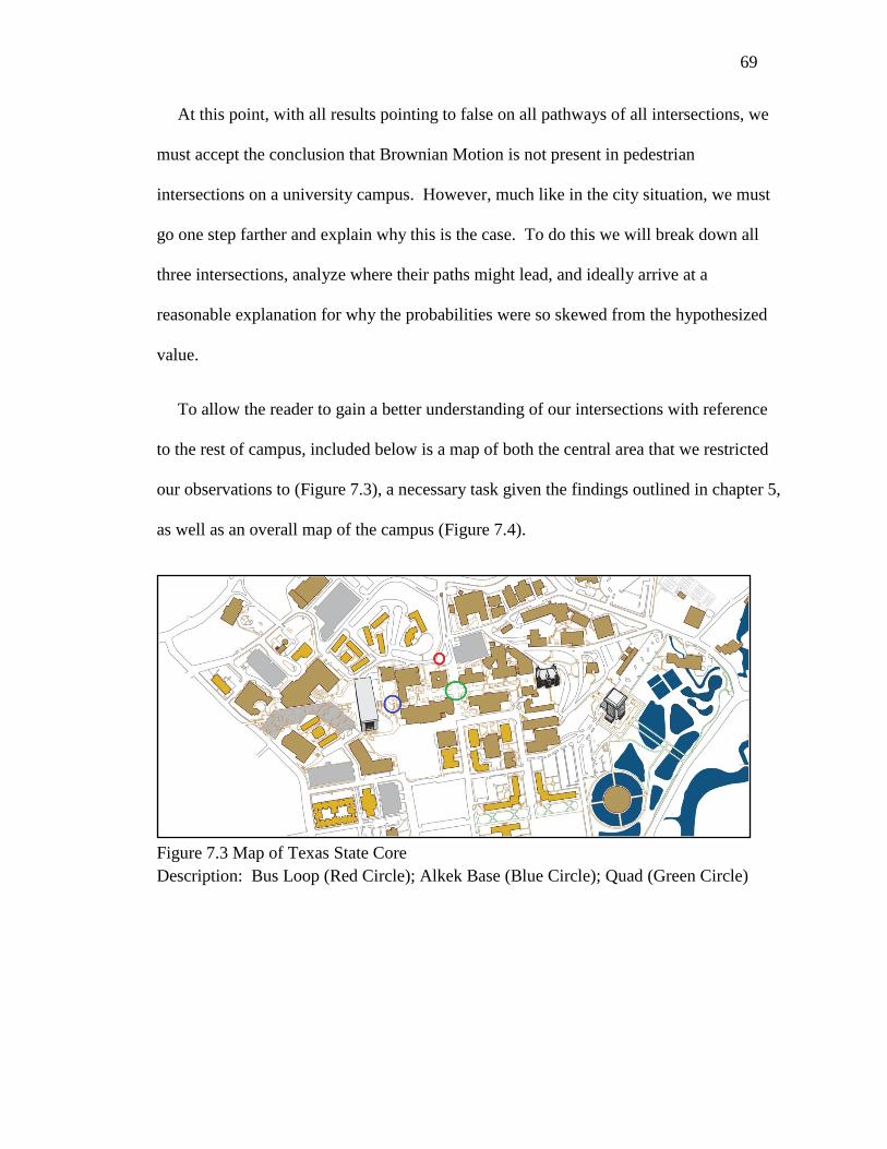
69
At this point, with all results pointing to false on all pathways of all intersections, we
must accept the conclusion that Brownian Motion is not present in pedestrian
intersections on a university campus. However, much like in the city situation, we must
go one step farther and explain why this is the case. To do this we will break down all
three intersections, analyze where their paths might lead, and ideally arrive at a
reasonable explanation for why the probabilities were so skewed from the hypothesized
value.
To allow the reader to gain a better understanding of our intersections with reference
to the rest of campus, included below is a map of both the central area that we restricted
our observations to (Figure 7.3), a necessary task given the findings outlined in chapter 5,
as well as an overall map of the campus (Figure 7.4).
Figure 7.3 Map of Texas State Core
Description: Bus Loop (Red Circle); Alkek Base (Blue Circle); Quad (Green Circle)

70
Figure 7.4 Map of Texas State Sections
Description: Figure 7.3 is bordered in red
The Bus Loop was the most extensively studied of the group, but at the same time is
the most reasonable to arrive at the conclusion we have drawn. All of our perspectives
will be specified in reference to the video’s view, but to state them plainly: Right led to
the line of busses commuting students to off campus locations; Up consisted of the
sidewalk and roadway leading up the hill towards Derrick Hall; Stairs was a pathway
leading off to the left; Ramp was a pathway also headed to the left, but whose exit was
Figure7.5 Bus Loop Image

71
distinctly different from Stairs. We will use these names in place of explaining the
pathway direction each time. It should be noted at this time that, though the percentages
may have varied from test to test, as did the population, the ranking of each probability in
terms of highest to lowest almost always remained the same.
Right was the clear choice for the majority of the population. As the name I have
given to the intersection suggests, the main reason that students would visit this pathway
is to access the busses for transportation purposes. At first, one might assume that the
probability would be the same since roughly the same number of students entering
campus by this method will also leave campus by this same method, however because
this is a four path intersection, that is not the case. All of the students entering by busses
have three unique options of where to go, while those preparing to leave campus only
have one pathway from this intersection that will end at the desired location. Beyond the
purpose of mass transportation, there is no other conceivable reason why a student would
choose this pathway, but as we saw in Chapter 5, transportation is a major influence on
where a person will walk.
The second strongest probability pathway went to the Ramp. This pathways was the
closest to reaching the desired percentage, and was close enough that we could not reject
the possibility of the true mean, or rather the average of all people to select that pathway,
to be twenty-five percent. However, because all four are required to meet this restriction
to be considered for a Brownian Motion, the test as a whole still failed.
The possible causes for Ramp being second were considerably less obvious based
upon the possible outcomes of the closely related Stairs, however upon closer inspection

72
the unexpected reasons become clear. Choosing the Ramp pathway is the shortest
distance to almost half of the buildings on campus. It also provides the shortest route to a
major commuter parking area by the tennis courts, a wide gently sloped pathway to the
Quad, though notably not the shortest, but most importantly, it is the quickest path to the
strip of busses serving all on-campus locations. From these busses, the students may
travel to the outlying commuter parking, multiple locations all over campus, the small
patch of green on campus, Sewell Park, and the Student Recreation Center. At this point,
from the earlier argument that most students entering campus by these busses are not very
likely to leave by some other method, the possibility of needing to travel to a commuter
lot cannot be ruled out simply by personal experience of having to leave my own car at
campus overnight for a variety of reasons. The secondary busses are still the most
important factor in this situation though, and it is because of the entertainment portion.
As was put forth as a hypothesis in the above City section of the data analysis, the
second most travelled pathway leads to a source of entertainment, we must view the few
locations the campus busses can lead to, the park and the recreation center. Whether it’s
a game of soccer, lifting weights, or relaxing by the river, these two places offer just
about any outdoor fun that can be desired inside of a large town. The Ramp pathway also
leads to the music building, which is frequently holding concerts, the photography and art
labs for those who enjoy taking photos, and my personal favorite, is the shortest pathway
to the off-campus coffee shops located just north of the traffic intersection.
The clear third choice in the ranking of the Bus Loop is the Up path. This pathway is
notably the largest simply to compensate for those students who would prefer to walk in a
rarely travelled road, which is unfortunately a common occurrence on our campus, than

73
continue on the distance farther to the stairs. Up provides the shortest distance to the
majority of Derrick Hall, a large grouping of dorm buildings, as well as every building
west of Alkek Library. If walking was the only method that had to be considered, then
this path would have been the clear second, but after analyzing the Ramp path, it is
clearer why the probabilities for this pathway were so severely decreased. Even though
the Up path does provided the shortest walking distance to half of campus, the Student
Rec Center, and a major parking area, only a few of the campus buildings can be reached
by walking from here easier than by travelling via a campus bus. Due to traffic on the
busses, walking is frequently the only option most students are willing to take, but the
traffic itself is proof enough that students are more willing to ride the bus if possible and
convenient enough.
The last pathway on the probability ranking for the Bus Loop was the Stairs path.
This pathway, while providing a shorter distance to the base of Derrick Hall as well as all
buildings in the main portion of campus east of Alkek, still fell far too short to be
competitive. I believe this is because:
1) The proportion of buildings are far too small to compare with Ramp and Up.
2) Stairs has very few or no sources of entertainment or places of mass
transportation.
Our next analysis will be of the intersection at the base of Alkek Library, which we
will call Alkek Base from here on. On the next page, figure 7.6, is an image of the
intersection at a single point in time during our observations.

74
Figure 7.6 Alkek Base Image
From the perspective of the footage, Up is the pathway leading towards Derrick Hall,
Right is the path directed down towards the Stallions statue and the Quad, Left leads to
the stairs headed up towards the library, and Down is a sidewalk towards a construction
area and will be the first pathway we analyze.
The Down pathway ends in a three-way intersection. To the left is a narrow sidewalk
that leads only to the Evans building, a building that can be reach much faster by
choosing Right instead. To the right of the t-intersection is yet another narrow pathway,
though this one leads up a set of stairs that snakes around to the other side of Alkek
Library. Due to construction, the stairs do not lead anywhere else, and so it is clear to see
that choosing Left would accomplish the same thing at a much shorter distance. This
being said, it is easy to see why Down was consistently the lowest ranking probability
choice. The second lowest was Up, and the reason is much easier to explain. Up is a

75
path that ends in MCS and Derrick Hall with only minor side paths that weave around the
building to the road behind. This same conclusion can be reached much faster and easier
by taking Left and then turning at another intersection closer to the library stairs.
The first and second highest probabilities of this intersection are the only ones in our
entire data set that varied enough to alter rankings from set to set. The Left and Right
pathways cumulative percentages swapped locations, and so to actually rank them farther
we must look at the averages. By this method, Right falls in third place, though this is
the first anomaly we have encountered. Using our earlier observations, it would appear
that, with this intersection being near center of campus and both pathways leading
towards half of the buildings on campus, that the decision would fall to the transportation
and entertainment aspects. However, with both the bus loop and the park planted to the
right, and only the Student Recreation Center and a bus stop, that is much farther away
than the bus loop, to the left, this decision clearly points to Right ranking above Left.
This prediction contradicts observed results though, leading to a probable combination of
one or more of three likely conclusions.
1) There is an unknown factor present on university campuses that is able to sway
population flow.
2) The results of the sample set of percentages of Right fell below the average of the
true population average.
3) The results of the sample set of percentages of Left fell above the average of the
true population average.

76
In any case, there is currently insufficient data from this intersection to draw a possible
conclusion of exactly what the cause is.
The final of our three intersections is the Quad. Of all three, this was the most closely
related to being a pure Brownian Motion, but even so, this intersection failed to meet the
most basic requirements. To provide the reader with a view of exactly where our paths
lead: Up leads towards Old Main; Right leads to Commons and The Square; Left leads to
the Bus Loop; Down leads towards The Stallions and Alkek Library. See figure 7.7
below.
Left, the obvious choice to be our top pathway because of the extremely close Bus
Loop, actually had the lowest average, however its rankings were more frequently in
Figure 7.7 The Quad Image
77
third place. This could imply that, on a university campus, buildings hold a larger pull
than transportation does on the students within our restricted times.
Up was ranked third on the list, though as can be implied from above, it was actually
ranked fourth in two of the three periods. In this intersection, this pathway provides the
shortest distance to roughly half of the academic buildings as well as one dining facility.
It is also the shortest pathway down to the Tennis Courts, which have a commuter
parking area, to Sewell Park, which was listed before as being a source of entertainment,
and to Bobcat Stadium, which houses the largest commuter parking area. With this
pathway meeting both of our major influences, it once again places doubt on our
conjectured influences, but places an even larger question in our minds. Exactly what is
pulling college students down one pathway or another?
The Down pathway was the most unlike a pure Brownian Motion because of its
unique consistency. Regardless of time, place, or weather conditions, this pathway was
always chosen the most frequently by a large margin. In two of our three observational
sessions, each of which lasted in excess of fifteen minutes, the difference in cumulative
percentages between this and the second highest rate was eleven percent. On the third
test, this difference jumped to twenty one percent. Besides being the shortest pathway to
approximately half of the buildings on campus, both academic and residential, none of
our other aforementioned influences are accessed via this route. At least, not at first
glance.
The only noticeable pull that this pathway might have is the large quantity of booths
and stands. The Quad is frequently home to a variety of student organizations trying to

78
gain new members, hosting fundraisers, or gaining support for a variety of events and
projects. While these booths may not be entertainment themselves, though occasionally
some are, they do provide a link to entertaining and motivational things. As students one
of our largest priorities should be education, and almost every organization, whether it be
fraternities, sororities, ROTC, or religious groups, stress education first and have
minimum GPA requirements. This is mostly due to the students needing to remain in
good standing with the university in order to remain in the groups, but still the motivation
is there.
Also, there is rarely a better way to meet new people and have fun gatherings than to
join an organization with other like-minded people. Therefore, even though these booths
themselves may not provide entertainment, I believe that the human mind is advanced
enough to realize that these booths provide a gamble for greater future experiences,
allowing us to label entertainment as a pull on this intersection.
Our second ranked intersection is the Right pathway, and of all four this intersection
had the highest likelihood of being a pure Brownian Motion. Its average percentage fell
at 25.38 and its t* value was such that we could not fully reject its true average
percentage. However, as was stated before, in order for a Brownian Motion to rule our
intersection, all of the pathways must meet this requirement. As such, this pathway still
fails.
Right leads to mostly residential buildings and a few dining facilities, but its largest
pull is likely to come from The Square. The Square is an area of San Marcos known to
have a very large variety of restaurants, stores, and shops. While it's true that we

79
exempted food from entertainment, this is could still be a major pull on students for two
main reasons. The first reason is that walking to town for sustenance provides a much
larger variety, as well as a higher quality, of food choices. The second reason is that,
disregarding those who bring their own lunches from home, the options off campus
provide larger portions for a lower cost.
A perfect example of this would be the Blimpie's on campus. Each meal trade costs
approximately five dollars, varying only slightly depending upon the size chosen, and one
meal trade earns a six inch sub, chips, and a soda. Meanwhile, there is a Subway just
south of campus that provides a foot long sub, chips, and a soda for only seven dollars
and twenty five cents. Furthermore, the Subway allows free refills while the Blimpie's
does not permit refills. Thus, for a one hundred percent increase in the size of the meal it
only took a fifty percent increase in cost. For a size to size match, Subway's six inch
subs, chips, and a drink only cost five dollars as well, but once again they permit free
refills. College students spend their days in class, their nights studying, and any free time
they have is split between sleep and work. It is here that we are likely to find the third
pull on college students that we could not determine in the City section, which I believe
is cost.
We will dwell here for a moment as we revisit a pathway from our first intersection,
the Ramp pathway in the Bus Loop intersection. While describing that pathway, we
made note that it was the fastest way to go off campus, and just like south of campus, the
north side has plenty of reasonably priced restaurants. Also like our Right pathway in the
Quad, the Ramp in the Bus Loop fell second in its ranking percentages, and neither could
reject the possibility of the true mean being twenty five percent, the desired average for

80
both intersections. The similarities between the two paths cannot be ignored, and if the
conjecture of cost being the third influence, it is here that we would determine it.
However, there are still too many variables to say exactly what pulls the students off
campus with a large amount of certainty. One example of this would be bookstores.
Both north and south of campus contain bookstores within walking distance, and both
locations sell books at a lower price than the university's. In this case, was it the cost
pulling the students, or could it actually have been the books? If we put forth the books
as being third in pull and cost, though still influential, farther down on our unknown list,
then it provides a much larger pull on the Down path of the Quad as well as explaining
why the Left path of the Alkek Base intersection rose above the Right pathway. In both
cases, Alkek Library and the University Bookstore can be reached with the least energy
by choosing these pathways. Adding in this possible influencer begins to bring a greater
cohesion into the results of our observations, providing greater support for adding books
into our hypothesized affecters.
§Conclusion
In this thesis, we explored the discovery of Brownian Motion, its founders, and even
some of its applications. We then moved into studying how Albert Einstein solved the
question of how to describe the motion, and viewed how his new perspective was
developed into a mathematical representation. We then moved into adapting his
Diffusivity Coefficient into our own theoretical one, showing how each constant related
to a constant in our own situation. Finally, we collected and analyzed our data, proving
false all three starting hypotheses:

81
1) In general, pedestrian movement at an intersection is not a Brownian Motion.
2) Pedestrian movement at intersections in high density cities is a Brownian Motion.
3) Pedestrian movement at intersections on a university campus during normal
business hours on normal business days is a Brownian Motion.
We then moved on to attempt to explain why the data moved the way it did. From the
city data, we were able to create two possible influencers, transportation and
entertainment, that seemed to explain the majority of the results. Once we viewed the
university scenario, we continued with the two city influencers, but were forced to create
two others, cost and books, to explain abnormalities that our earlier affecters could not
account for.
Due to restrictions in time and data, we were not able to place numbers for exactly
how much these influencers pull pedestrian movement down one pathway or another. In
the university case we were unable to even determine an appropriate ranking for which
have the greatest pull and which are only mildly important. Future research could
alleviate this problem, and therein create a simple pedestrian movement mapping that
could label where a random person is most likely to walk to and with what probability.
This could even branch out to explaining animal movement, and why some animals will
choose one pathway to migrate one year, and then entirely changes for the next. Only
one thing can be assured from this research, that the future holds infinite possibilities.

82
BIBLIOGRAPHY
"Albert Einstein-Biography." Nobelprize.org
http://www.nobelprize.org/nobel_prizes/physics/laureates/1921/einstein-bio.html
(accessed November 29, 2011)
American Diabetes Association. " The Role of Free-Living Daily Walking in Human
Weight Gain and Obesity: Results" Medscape Today News.
http://www.medscape.com/viewarticle/572997_3 (accessed November 20, 2011)
American Institute of Physics. “Einstein on Brownian Motion.” Einstein and Our World.
http://www.aip.org/history/einstein/essay-brownian.html (accessed October 10,
2011)
Bassett, David R. Jr., Andra L. Cureton, Barbara E. Ainsworth.
"Measurement of daily walking distance-questionnaire versus pedometer."
Medicine and Science in Sports and Exercise. http://journals.lww.com/acsm-
msse/Abstract/2000/05000/Measurement_of_daily_walking.21.aspx
(accessed November 25, 2011)
Blauch, David N. "Kinetic Molecular Theory." Davidson University.
http://www.chm.davidson.edu/vce/kineticmoleculartheory/BasicConcepts.html
(accessed November 19, 2011)
Brix, Anders, Stephen Jewson, and Christine Ziehmann. Weather Derivative Valuation:
The Meteorological, Statistical, Financial, and Mathematical Foundations.
Cambridge, United Kingdom: Cambridge University Press, 2005
Burgess, Ernest W. The Growth of the City: An Introduction to a Research Project.
Boston, MA: Ardent Media, 1967

82
Chamness, Brenda, et al. "American Fitness Index-2011."
American College of Sports Medicine.
http://www.americanfitnessindex.org/docs/reports/2011_afi_report_final.pdf
(accessed November 25, 2011)
Chamness, Brenda, et al. "American Fitness Index-2011."
American College of Sports Medicine.
http://www.americanfitnessindex.org/docs/reports/2011_afi_report_final.pdf
(accessed November 25, 2011)
Chen, C. C., J. S. Daponte, and M. D. Fox.
"Fractal feature analysis and classification in medical imaging."
IEEE Trans Med Imaging. http://www.ncbi.nlm.nih.gov/pubmed/18230510
(accessed October 24, 2011)
Einstein, Albert. Investigations on the Theory of the Brownian Movement.
New York, NY: Dover Publications, 1956
"The Equipartition Theorem." Department of Chemistry, Oxford University.
http://vallance.chem.ox.ac.uk/pdfs/Equipartition.pdf (accessed October 3, 2011)
Goodman, Jonathan. "Stochastic Calculus Lecture 7." New York University
http://www.math.nyu.edu/faculty/goodman/teaching/StochCalc/notes/l9.pdf
(accessed November 16, 2011)
Grupo de Fisica Matematica da Universidade de Lisboa.
“Uses of Brownian Motion in Brain Imaging and Neuroscience.” GFM Seminar.
http://gfm.cii.fc.ul.pt/events/seminars/20070614-lori (accessed October 10, 2011)
Huang, Rongxin, I. Chavez, K. Tuate, B. Lukic, S. Jeney, M. Raisen, And E. Florin.
"Direct observation of the full transition from ballistic to diffusive Brownian
Motion in a liquid". Nature Physics. http://chaos.utexas.edu/wp-
uploads/2011/02/27.-2011-Nature-Physics.pdf (accessed October 31, 2011)
Imperial College of London. “Applications of Brownian Motion: Article Two.” Surprise
95. http://www.doc.ic.ac.uk/~nd/surprise_95/journal/vol2/ykl/article2.html
(accessed October 10, 2011)

82
Imperial College of London. “Brownian Motion: The Research Goes on.” Surprise 95.
http://www.doc.ic.ac.uk/~nd/surprise_95/journal/vol4/ykl/report.html
(accessed October 10, 2011).
Jack Song. "Dogenzaka in Shibuya: Tokyo's Hippest Entertainment District." Asiagate.
http://goldsea.com/Asiagate/Entertainment/tokyo.html (accessed January 30,
2012)
Li, Huan, Robert Bertini. "Optimal Bus Stop Spacing for Minimizing Transit Operation
Cost." Department of Civil and Environmental Engineering,
Portland State University.
http://www.its.pdx.edu/upload_docs/1248894217RWAeWSDYZ9.pdf
(accessed November 25, 2011)
"List of Largest Colleges and Universities." CollegeStats.org.
http://collegestats.org/colleges/all/largest (accessed November 25, 2011)
Merriam Webster. “Stochastic.” Dictionary.
http://www.merriam-webster.com/dictionary/stochastic (accessed October 10,
2011)
Planning Commission Committee. "Walking Distance Research."
Fairfax County Department of Transportation.
http://www.fairfaxcounty.gov/planning/tod_docs/walking_distance_abstracts.pdf
(accessed November 20, 2011)
Prof. Brian J. Ford Website.
“Brownian Movement in Clarkia Pollen: A Reprise of the First Observations.”
Ford, Brian J. http://www.sciences.demon.co.uk/wbbrowna.htm
(accessed October 10, 2011)
Renn, J. A Einstein's Invention of Brownian Motion. Berlin, Germany: Leipzig, 2005
Short, Nicholas M. "Vegetation Applications." NASA.
http://rst.gsfc.nasa.gov/Sect3/Sect3_1.html (accessed November 20, 2011)

82
Spies, Maria "Macroscopic Theory of Diffusion." Department of Biophysics,
University of Illinois
http://www.life.illinois.edu/biophysics/401/Files/083111notes.pdf
(accessed October 10, 2011)
Stachel, John. Einstein's Miraculous Year. Princeton, NJ:
Princeton University Press, 1998
Stephens, W. B. "A History on the County of Warwick Volume 7: The City of
Birmingham." Victoria County History. http://www.british-
history.ac.uk/report.aspx?compid=22959 (accessed November 20 2011)
US Naval Research Laboratory. “Brownian Motion In The Stock Market.” Operations
Research.http://www.e-m-h.org/Osbo59.pdf (accessed October 10, 2011)
Vallee, Robert. "Norbert Wiener-Biography." International Society for the Systems
Sciences. http://www.isss.org/lumwiener.htm (accessed November 28, 2011)

VITA
Jonathan Turner was born in Southbend, Indiana, on October 29, 1989. After he
completed his Bachelor of Science in Mathematics at Texas State Univeristy-San Marcos
in May, 2011, he immediately enrolled in the Graduate College of Texas State.
Email Address: [email protected]
This thesis was typed by Jonathan S. Turner.