Bridging the Gap Between Neural Networks and NeuromorphicHardware with A Neural Network Compiler

Yu Jijiy15@mails.tsinghua.edu.cn

Department of Computer Science and TechnologyTsinghua University

China

Youhui Zhang∗zyh02@tsinghua.edu.cn

Department of Computer Science and TechnologyTsinghua University

China

Wenguang Chencwg@tsinghua.edu.cn

Department of Computer Science and TechnologyTsinghua University

China

Yuan Xieyuanxie@ece.ucsb.edu

Department of Electrical and Computer EngineeringUniversity of California at Santa Barbara

USA

ABSTRACTDifferent from developing neural networks (NNs) for general-purposeprocessors, the development for NN chips usually faces with somehardware-specific restrictions, such as limited precision of networksignals and parameters, constrained computation scale, and limitedtypes of non-linear functions.

This paper proposes a general methodology to address the chal-lenges. We decouple the NN applications from the target hardwareby introducing a compiler that can transform an existing trained,unrestricted NN into an equivalent network that meets the givenhardware’s constraints. We propose multiple techniques to makethe transformation adaptable to different kinds of NN chips, andreliable for restrict hardware constraints.

We have built such a software tool that supports both spikingneural networks (SNNs) and traditional artificial neural networks(ANNs). We have demonstrated its effectiveness with a fabricatedneuromorphic chip and a processing-in-memory (PIM) design. Testsshow that the inference error caused by this solution is insignificantand the transformation time is much shorter than the retrainingtime. Also, we have studied the parameter-sensitivity evaluationsto explore the tradeoffs between network error and resource utiliza-tion for different transformation strategies, which could provideinsights for co-design optimization of neuromorphic hardware andsoftware.

KEYWORDSNeural Network, Accelerator, Compiler

1 INTRODUCTIONDesigning custom chips for NN applications with the Very-Large-Scale-Integration (VLSI) technologies has been investigated as apower-efficient and high-performance alternative to general-purposecomputing platforms such as CPU and GPU. However, program-ming these chips is difficult because of some hardware-specificconstraints: 1○ Due to the utilization of hardware resources fordigital circuits or the capability of analog computing for some mem-ristor-based designs [18, 31, 40, 44, 55], the precision of input and

∗Corresponding author

output signals of neurons is usually limited, as well as 2○ the preci-sion of NN parameters, such as synaptic weights. 3○ The presentfabrication technology limits the fan-in and fan-out of one neuron,which constrains the computation scale. 4○ The diversity of nonlin-ear functions or neuron models supported by the hardware is alsolimited. For example, for TrueNorth chips [52], the maximum ma-trix that one synaptic core can handle is 256 × 256, and it supportsonly a simplified leaky–integrate-and-fire (LIF) neuron model.

One straightforward approach to this problem is to expose thehardware details and limitations to the NN developer directly. Forinstance, IBM has provided a TrueNorth-specific training mecha-nism [22]. The mechanism constructs the whole NN model fromscratch to satisfy all hardware limitations, and then trains the NNmodel. This method has several drawbacks. First, it binds NN mod-els to the specific target hardware. Developers can hardly benefitfrom existing NN models from the machine-learning community.Second, it limits the power of the NN algorithm. The constraintsmake it more difficult to converge and reach better accuracy forlarger models. Third, training the specific NN model from scratchmay take a very long time.

Another approach is to make hardware satisfy software require-ment by consuming more hardware resources to reduce the con-straints on NNmodels [12, 15, 21, 47], such as using 16-bit precisionrather than 1-bit spiking signals in TrueNorth. This approach cangain less performance improvement fromNN quantization and com-pression technologies. For some memristor-based designs, someconstraints due to analog computing are physical limitations, whichare difficult to overcome even with more hardware resources con-sumed.

A third approach is to introduce a domain-specific Instruction SetArchitecture (ISA) for NN accelerators, such as the Cambricon [48]ISA. This approach requires both hardware and software to satisfythe ISA. However, this approach still does not solve the gap betweenprogramming flexibility required by NNs and hardware efficiencythat can be gained from NNs’ redundancy. If we use high-precisioninstructions that do not have any constraints, the hardware cangain less benefit from NN’s redundancy. In contrast, if we use low-precision instructions with many constraints, the NN developershould take these constraints into consideration when developingNN models.

1

arX

iv:1

801.

0074

6v3

[cs

.NE

] 1

8 Ja

n 20

18

In addition to these approaches, there are also some work toutilize the NNs’ redundancy for performance and provide flexibleprogramming interface by introducing a transforming procedure.EIE [27] is such an instance: it extensively uses deep compressionto squeeze the redundancy, and design custom chip, EIE, to runthe compressed NN model. NEUTRAMS [35] also use NNs’ redun-dancy to adapt the original model to satisfy hardware constraints.However, these methods highly depends on the redundancy in NNmodels. Different NN models may have different minimum require-ment (precision, connectivity, etc.) on hardware. Thus, transformingprocedure is not a general method, especially for NN models withless redundancy and hardware with severe constraints.

In this paper we propose a new method with flexibility, betterapplicability, and easy convergence. First, we decouple the neu-romorphic computer system into two levels for better flexibility,software programming model and hardware execution model. Weuse computational graph (CG), which is widely used in many pop-ular NN frameworks [1, 4, 36], as the programming model for NNmodels. We also provide the hardware/software (HW/SW) interfaceand the minimum hardware functionality that an NN hardwareshould provide. We propose a transformation workflow to converta trained NN, expressed as a CG, into an equivalent representationof HW/SW interface through the fine-tuning method.

To make the transformation workflow general and reliable fordifferent cases, we employed two principles.• Trade Scale for Capability. As the operations supported by NNhardware is not comparable to their software counterparts dueto the constraints, it is reasonable to enlarge the graph scale andcomplicate the topology properly to improve the model capability,especially under strict conditions.• Divide and conquer.We fine-tune the entire model part by partaccording to a topological ordering. Each part is a smaller graph thatis more easier to converge. We also fine-tune each part with severalphases to introduce different constraints, which also facilitates thefast convergence.

Moreover, this transformation procedure could be viewed ascompilation of traditional computer systems that converts high-level programs (the hardware-independent, trained NNmodels) intoinstructions that hardware can understand (the SW/HW interface),and the transformation tool could be called an NN compiler. As asummary, this paper has achieved the following contributions:• An NN transformation workflow is presented to complete the

aforementioned technologies to support different types of NNs.The SW/HW interface is easy to be adapted to different NNhardware.

• Such a toolchain is implemented to support two different hard-ware designs’ constraints, a real CMOS neuromorphic chip forANN&SNN, TianJi [60], and a PIM design built upon metal-oxideresistive random access memory (ReRAM) for ANN, PRIME [18].

• We complete quite a few evaluations of various metrics. The extraerror caused by this process is very limited and time overhead ismuch less (compared to the whole training process of the originalNN). In addition, its sensitivity to different configurations andtransformation strategies has been explored comprehensively.

2 BACKGROUND2.1 NN basisNNs are a set of algorithms, modeled loosely after the human brain,that are designed to recognize patterns. Traditional NNs consist ofmultiple layer of neurons. Each layer performs the computation asshown in Equation 1 where X is the input vector, Y is the outputvector,W is the weight matrix, B is the bias, and σ is a non-linearactivation function, which is typically the Rectified Linear Units(ReLU) function [54].

Y = σ (W · X + B) (1)

This kind of NN is also known as multilayer perceptron (MLP),which has been proved to be a universal approximator [30]. Mod-ern NNs are more complicated. The topology is a graph rather thana simple chain, and the types of operations are richer than matrix-vector multiplication. Most deep learning frameworks [1, 2, 4, 13]use computational graph (CG), a directed acyclic graph, to repre-sent NN computations. Vertices in the graph represent operations(e.g., dot-product, convolution, activation function, pooling) andimmutable/mutable states [1] (e.g., the weight parameters associ-ated). Edges represent the data dependency between vertices. Bothvertices and edges process or carry tensor data (multi-dimensionalarrays).

For clarity, in this paper, dot-product, bias-addition, and con-volution are categorized as weighted-sum operations. Moreover,any constant operand, including the trained weight matrix for anyvertex of weighted-sum operation, is considered as part of the cor-responding vertex as we can view it as the immutable state of thevertex.

2.2 NN ChipsThere are two types of NN chips. The first type focuses on thetraditional ANNs. They are custom architectures [11, 12, 15, 21, 23,24, 38, 39, 46, 47, 56, 57, 59, 61, 64, 67, 68] to accelerate mature ANNmodels. We usually call this type NN accelerators. The second isneuromorphic chips, which usually supports SNNs to yield higherbiological reality [7, 9, 10, 25, 51, 52, 60, 66].

These chips usually consist of a lot of processing elements (PEs)that can efficiently perform dot-product operations because thisoperation is the main body of most NN models. Different chips putdifferent constraints on the operations they support. Table 1 showsthe constraints of some existing NN chips. Most NN chips employlow precision numbers to represent weights and input/output (I/O)data instead of floating-point numbers. The scale of computationthat each PE can process is usually fixed. PRIME [18] and Dian-Nao [12] have extra adders to support larger scale computations.However, NN chips such as TianJi [60] and TrueNorth [52] do nothave extra adders, and the output of their PE can connect to onlyone input port of another PE. For these chips, the scale of computa-tion is also a problem. Despite the widely-supported dot operation,many other operations required by NNs usually lack for support.

3 PROBLEM DESCRIPTIONTo bridge the gap between NN applications and NN chips, we de-couple the whole system stack with a software programming modeland a hardware execution model. The former is the programming

2

Chip Weight I/O Scale NonlinearTianJi [60] 8-bit 8-bit 2562 ConfigurablePRIME [18] 8-bit 6-bit 2562 ReLU

Max PoolingDianNao [12] 16-bit 16-bit 162 ConfigurableTPU [37] 8-bit 8-bit None ReLU

Max Poolingetc.

TrueNorth [52] 2-bit Spiking 2562 LIFTable 1: Hardware limitations of NN chips

interface for NN experts to develop NN applications. The later isthe SW/HW interface that NN chips can executed directly.Software Programming Model. The machine-learning commu-nity has already employed Computational Graph (CG) as the pro-gramming model. It is a data-flow graph G = (V ,E) which repre-sents a number of operations with vertices V and represents datadependencies between these operations with edges E. Most deep-learning frameworks [1, 2, 4, 13] adopt CG to build NNmodels. Andthe set of supported operations is F .

Each vertex in V is an operation y = f (x1, . . . ,xn ), where f ∈F , y represents the output edge, and {x1, . . . ,xn } represent inputedges. Thus, the entire model can be expressed as a compositefunction Y = H (X ), where X represent all input vertices and Yrepresents all output vertices.

We also adopt CG as the programming model with a slight mod-ification. The difference is that we regard model parameters asimmutable states of the corresponding vertices instead of normaledges of the vertices. Namely, we regard an operation f (x ,θ ) asf θ (x), where θ is model parameters and x is an input operand.Thus, it can only be a trained NN model that all parameters havebeen already determined.Hardware Execution Model. The computation model that hard-ware could execute is also a data-flow graph G ′ = (V ′,E ′). It has asupported operation set F ′, denoted as core-op set. However, the sup-ported operations are very limited, and these operations have manylimitations. In addition, some hardware also has constraints onthe interconnection subsystem. For example, TianJi and TrueNorthdoes not support multi-cast; one output port of each PE can only beconnected to one input port. The hardware execution model formsa composite function Y ′ = H ′(X ′).

Thus, our goal is to build G ′ from G so that H ′ is approximatelyequivalent to H .MinimumHardware Requirement.We define a minimum set ofoperationsC thatC ⊂ F ′ has to be satisfied to use our NN compiler.It only contains one operation, denoted as dot–core-op. Namely, theoperation dot–core-op must belong to the core-op set. Equation 2shows the computation of the dot–core-op where X and Y are theinput and output vectors, respectively; N andM are their sizes;Wis the weight matrix of sizeM × N ; and σ is a nonlinear activationfunction.

Yj = σ (∑iWjiXi ) (1 ≤ j ≤ M, 1 ≤ i ≤ N ) (2)

In addition, the I/O data precision is B bits.

Formally, the dot–core-op meets the following constraints:• N ,M ,B are fixed.• The value range of each element inW is a finite set S . S iseither a fixed set or a configurable set SP with some param-eters P .

• Without loss of generality, only ReLU function (σ ) is sup-ported.

We choose this dot–core-op as the minimum requirement forhardware because it can cover most existing NN chips (e.g., thoselisted in Table 1). Thus, our NN compiler can support most existingNN chips.

4 TRANSFORMATION METHODOLOGYIn this section, wewill introduce the transformationmethodology totransform the software programming model into an approximatelyequivalent hardware execution model.

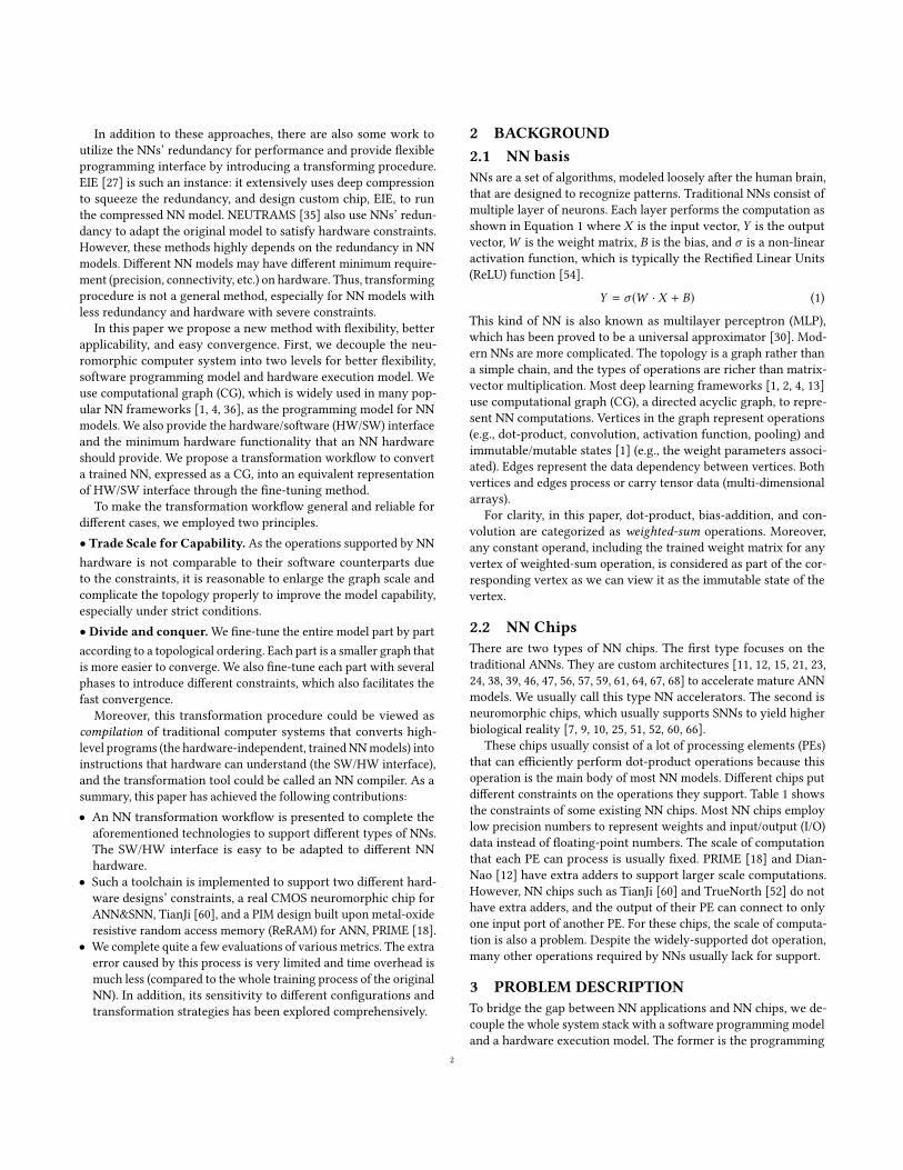
4.1 The workflow outlineThe proposed workflow involves 4 steps as shown in Figure 1.

Build

Model Information

Computational Graph

Graph Reform

Computational Graph with core_op-like operations

Graph Tuning

Computational Graph with only core_ops

Mapping

Chip configuration

FreeTuning

Value Range Tuning

RoundingTuning

Data Re-encoding

Fully Expanding

Weight Tuning

Figure 1: Workflow of our proposal, from the input modelto the output for chip. Step ‘Graph Tuning’ contains 3 sub-steps for different hardware restrictions respectively andthe third sub-step has 3 fine-tuning phases.

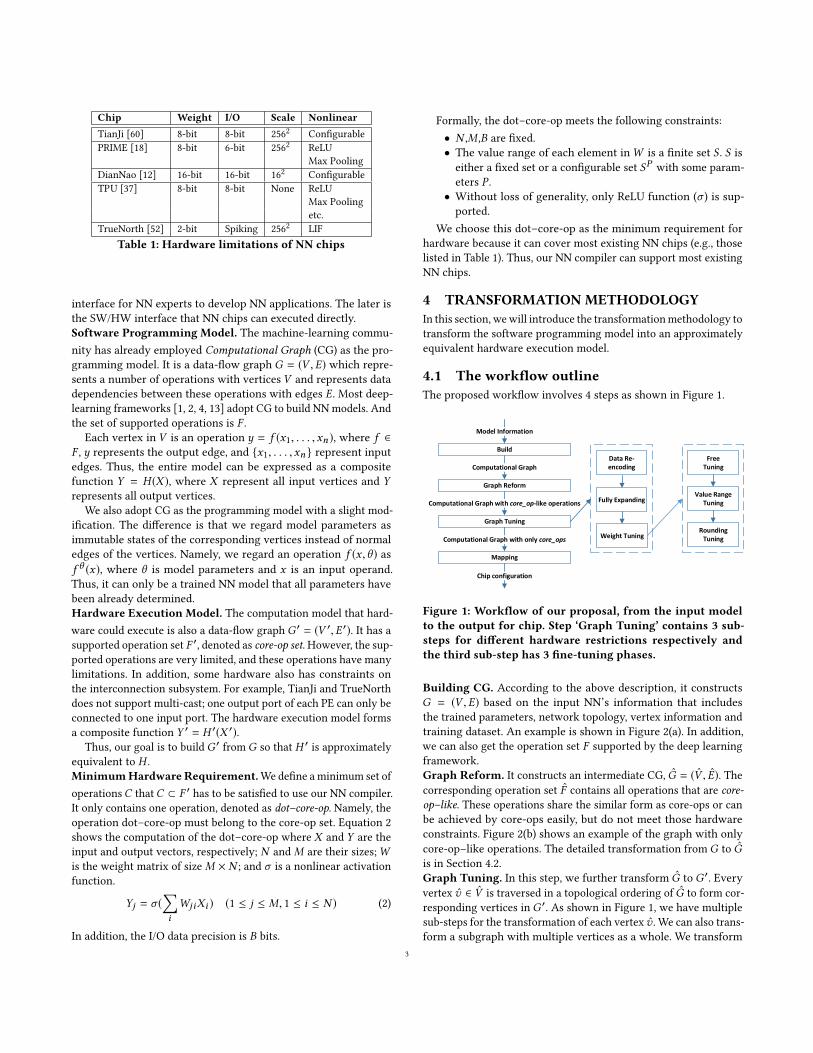
Building CG. According to the above description, it constructsG = (V ,E) based on the input NN’s information that includesthe trained parameters, network topology, vertex information andtraining dataset. An example is shown in Figure 2(a). In addition,we can also get the operation set F supported by the deep learningframework.Graph Reform. It constructs an intermediate CG, G = (V , E). Thecorresponding operation set F contains all operations that are core-op–like. These operations share the similar form as core-ops or canbe achieved by core-ops easily, but do not meet those hardwareconstraints. Figure 2(b) shows an example of the graph with onlycore-op–like operations. The detailed transformation from G to Gis in Section 4.2.Graph Tuning. In this step, we further transform G to G ′. Everyvertex v ∈ V is traversed in a topological ordering of G to form cor-responding vertices in G ′. As shown in Figure 1, we have multiplesub-steps for the transformation of each vertex v . We can also trans-form a subgraph with multiple vertices as a whole. We transform

3

Input

Conv(weight)

Add(Bias)

ReLU

Max Pooling

...

Dot(weight)

Add(Bias)

ReLU

...

Output

Input

Conv(weight)

Add(Bias)

ReLU

...

Dot(weight)

Add(Bias)

ReLU

...

Output

ReLU

Dot

ReLU

Dot

ReLU

Dot

ReLU

Dot

Input

...

...

Output

ReLU

Dot

ReLU

Dot

ReLU

Dot

ReLU

Dot

ReLU

Dot

ReLU

Dot

ReLU

Dot

ReLU

Dot

ReLU

Dot

ReLU

Dot

ReLU

Dot

ReLU

Dot

ReLU

Dot

ReLU

Dot

ReLU

Dot

ReLU

Dot

ReLU

Dot

ReLU

Dot

ReLU

Dot

ReLU

Dot

Original CG Intermediate CG CG with core-ops

(a) (b) (c)

Figure 2: A transformation example

the whole graph part by part to have a better convergence sincesmaller graph are easier to be approximated. It is where we employthe divide-and-conquer principle. The sub-steps are as following.

• Data Re-encoding. Re-encode I/O data on each edge of thesubgraph to solve the precision problem of I/O data. Thissub-step is where we employ the trade-scale-for-capabilityprinciple. It enlarges the computation scale, but does notchange the operation type, each vertex is still a core-op–likeoperation.

• Fully Expanding. Since core-op–like operations are easyto be implemented with core-ops, in this sub-step, we fullyexpand each core-op–like operation with multiple core-opoperations to solve the limitation on the computation scale.After this sub-step, the subgraph only contains core-ops.

• Weight Tuning. This step aims to fine-tune the weightmatrices of core-ops in the subgraph to minimize transfor-mation error, under the premise of satisfying the hardwareweight precision. As shown in Figure 1, we also introducethree phases of fine-tuning to make it more reliable andeasier to converge. It is also where we employ the divide-and-conquer principle.

Figure 2(c) shows an example of the transformed graph G ′ withonly core-ops. Detailed transformation are in Section 4.3.Mapping. Now we have built an equivalent Graph G ′ with onlycore-ops that meet hardware constraints, which will be mappedonto the target hardware efficiently. This part highly depends on thehardware’s interconnection implementation. In Section 4.4 we will

introduce the basic principle of mapping the hardware executionmodel onto target chips.

4.2 Graph ReformIn this step, we need to transform a CGG into a graph G with onlycore-op–like operations. The operation set F includes all operationsthat could be combined by core-ops in F ′ without any precisionconstraints. For example, the corresponding core-op–like opera-tions for dot–core-op are all operations that in the form of weightedsum with activation function, denoted as dot-like operations.

To replace all vertices represented with F into operations in F ,we take the following three steps in order.

1○ First, we find all subgraphs that match the computationof any f ∈ F , and replace them with f . For example, inFigure 2(b), we merge the dot-product, add-bias and ReLUoperations into one operation, which is a dot-like operation.

2○ Then, we can also have some customized mapping from asubgraph in G into a subgraph formed of operations in F ,and apply these dedicated designs here. For example, max-pooling operation can be built with max functions. A simplemax function with two operands can be achieved with asEquation 3, which includes multiple dot-like operations.

max(a,b) =12[ReLU(a + b) + ReLU(a − b)

+ReLU(−a + b) + ReLU(−a − b)](3)

We can use the max function with two operands to form maxfunction with more operands.

3○ Finally, for the left operations in G, we provide a defaulttransformation strategy: we use multiple dot-like operationsto form MLPs to approximate them since MLP is proved tobe an universal approximator [30].

After the transformation, we form an graph G with only core-op–like operations.

4.3 Graph TuningIn this step, we transform the intermediate graph G = (V , E) tothe hardware execution model G ′ = (V ′,E ′). We use the originalgraph G to supervise the fine-tuning progress of the generatedG ′. The graph G can provide not only labels of the output butalso supervised signals of all intermediate data between operations.Each edge e ∈ E can provide supervised signal for graph G ′. Thus,we can split G into parts, and transform it intoG ′ part by part. To doso, first we find the edges e ∈ E that correspond to the edges e ∈ E,and use them to split the graph G . Then, we perform the followingsteps against each part one by one in a topological ordering of G.Note that, we can also transform multiple adjacent parts as a wholeeach time.•DataRe-encoding. Since the originalmodelG usually use floating-point numbers for computation and data representation, directlyrounding data to hardware I/O precision may distort and lost infor-mation. Thus, this sub-step aims to re-encode the input and outputdata of each vertex. To encode a floating-point vector with a low-precision vector, we employ an autoencoder to get the low-precisionrepresentation.

4

Input

Conv(weight)

Add (Bias)

ReLU

...

Dot (weight)

Add (Bias)

ReLU

...

Output

Input

...

Output

ReLU

Dot

ReLU

Dot

ReLU

Dot

ReLU

Dot

ReLU

Dot

ReLU

Dot

ReLU

Dot

ReLU

Dot

Dot (weight)

Add (Bias)

ReLU

...

Dot (decoder)

Input

...

Output

ReLU

Dot

ReLU

Dot

ReLU

Dot

ReLU

Dot

ReLU

Dot

ReLU

Dot

ReLU

Dot

ReLU

Dot

...

Dot (decoder)

Dot (encoder)

Add (Bias)

Round

Dot (decoder)

Hardware I/O precision

Input

...

Output

ReLU

Dot

ReLU

Dot

ReLU

Dot

ReLU

Dot

ReLU

Dot

ReLU

Dot

ReLU

Dot

ReLU

Dot

Dot (weight)

...

Dot (decoder)

Dot (encoder)

Add(new Bias)

Round

Dot (decoder)

Hardware I/O precision

Input

...

Output

ReLU

Dot

ReLU

Dot

ReLU

Dot

ReLU

Dot

ReLU

Dot

ReLU

Dot

ReLU

Dot

ReLU

Dot

...

Hardware I/O precision

Dot(new W)

Add(new Bias)

Round

Dot (decoder)

Hardware I/O precision

Input

...

Output

ReLU

Dot

ReLU

Dot

ReLU

Dot

ReLU

Dot

ReLU

Dot

ReLU

Dot

ReLU

Dot

ReLU

Dot

...

Dot (decoder)

ReLU

Dot

ReLU

Dot

ReLU

Dot

ReLU

Dot

ReLU

Dot

ReLU

Dot

ReLU

Dot

ReLU

Dot

Hardware I/O precision

Hardware I/O precision

Input

...

...

Output

Error

Product

Fully

expand

Fin

e-tu

nin

g

(a) (b) (c) (d) (e) (f)

Insert

(g)

Dot (weight)

Add (Bias)

ReLU

Merge

into

Conv(weight)

Add(Bias)

ReLU

Dot (weight)

Add(Bias)

ReLU

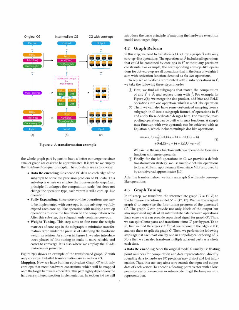
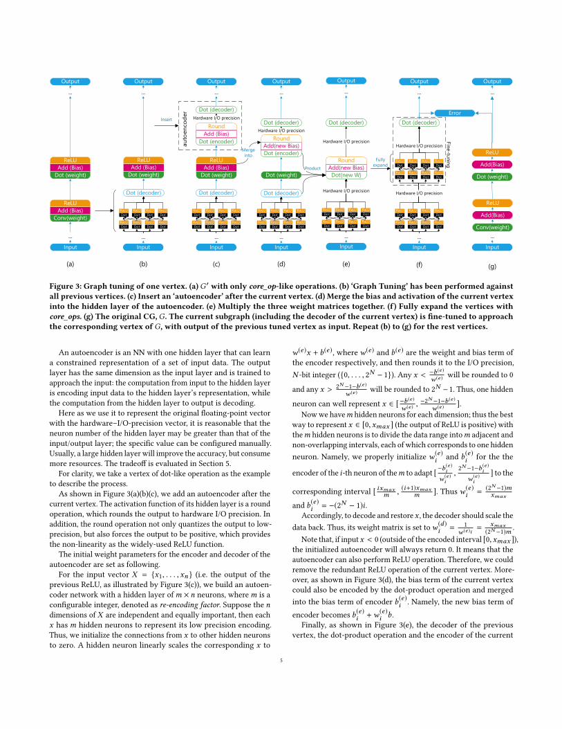
Figure 3: Graph tuning of one vertex. (a)G ′ with only core_op-like operations. (b) ‘Graph Tuning’ has been performed againstall previous vertices. (c) Insert an ‘autoencoder’ after the current vertex. (d) Merge the bias and activation of the current vertexinto the hidden layer of the autoencoder. (e) Multiply the three weight matrices together. (f) Fully expand the vertices withcore_ops. (g) The original CG,G. The current subgraph (including the decoder of the current vertex) is fine-tuned to approachthe corresponding vertex of G, with output of the previous tuned vertex as input. Repeat (b) to (g) for the rest vertices.

An autoencoder is an NN with one hidden layer that can learna constrained representation of a set of input data. The outputlayer has the same dimension as the input layer and is trained toapproach the input: the computation from input to the hidden layeris encoding input data to the hidden layer’s representation, whilethe computation from the hidden layer to output is decoding.

Here as we use it to represent the original floating-point vectorwith the hardware–I/O-precision vector, it is reasonable that theneuron number of the hidden layer may be greater than that of theinput/output layer; the specific value can be configured manually.Usually, a large hidden layer will improve the accuracy, but consumemore resources. The tradeoff is evaluated in Section 5.

For clarity, we take a vertex of dot-like operation as the exampleto describe the process.

As shown in Figure 3(a)(b)(c), we add an autoencoder after thecurrent vertex. The activation function of its hidden layer is a roundoperation, which rounds the output to hardware I/O precision. Inaddition, the round operation not only quantizes the output to low-precision, but also forces the output to be positive, which providesthe non-linearity as the widely-used ReLU function.

The initial weight parameters for the encoder and decoder of theautoencoder are set as following.

For the input vector X = {x1, . . . ,xn } (i.e. the output of theprevious ReLU, as illustrated by Figure 3(c)), we build an autoen-coder network with a hidden layer ofm × n neurons, wherem is aconfigurable integer, denoted as re-encoding factor. Suppose the ndimensions of X are independent and equally important, then eachx hasm hidden neurons to represent its low precision encoding.Thus, we initialize the connections from x to other hidden neuronsto zero. A hidden neuron linearly scales the corresponding x to

w(e)x + b(e), where w(e) and b(e) are the weight and bias term ofthe encoder respectively, and then rounds it to the I/O precision,N -bit integer ({0, . . . , 2N − 1}). Any x < −b (e )

w (e ) will be rounded to 0

and any x > 2N −1−b (e )

w (e ) will be rounded to 2N −1. Thus, one hidden

neuron can well represent x ∈ [−b (e )

w (e ) ,−2N −1−b (e )

w (e ) ].Nowwe havem hidden neurons for each dimension; thus the best

way to represent x ∈ [0,xmax ] (the output of ReLU is positive) withthem hidden neurons is to divide the data range intom adjacent andnon-overlapping intervals, each of which corresponds to one hiddenneuron. Namely, we properly initialize w(e)

i and b(e)i for the the

encoder of the i-th neuron of them to adapt [−b(e )i

w (e )i

,2N −1−b (e )

i

w (e )i

] to the

corresponding interval [ ixmaxm ,

(i+1)xmaxm ]. Thus w(e)

i =(2N −1)mxmax

and b(e)i = −(2N − 1)i .Accordingly, to decode and restorex , the decoder should scale the

data back. Thus, its weight matrix is set tow(d )i = 1

w (e )i =xmax

(2N −1)m .Note that, if inputx < 0 (outside of the encoded interval [0,xmax ]),

the initialized autoencoder will always return 0. It means that theautoencoder can also perform ReLU operation. Therefore, we couldremove the redundant ReLU operation of the current vertex. More-over, as shown in Figure 3(d), the bias term of the current vertexcould also be encoded by the dot-product operation and mergedinto the bias term of encoder b(e)i . Namely, the new bias term ofencoder becomes b(e)i +w

(e)i b.

Finally, as shown in Figure 3(e), the decoder of the previousvertex, the dot-product operation and the encoder of the current

5

vertex can be merged as one dot-product operation, whose weightmatrix is the product of the three’s matrices.

Till now, the input and output of the current vertex have beenconstrained to hardware I/O precision.

For vertices of convolution plus activation function, the processis similar. Instead of using dot-product operation as encoder anddecoder, we use convolution instead, and the three convolutionscan be merged into one as well. The initialization is also similar:the hidden layer hasm channels for each input channel, and onlythe center value of the encoder/decoder kernel is set to non-zero.

Owing to this step, we solve the limitation problem of I/O pre-cision. In this step, we only change the computation scale of theoperations in G.• Fully Expanding. In this step, we will turn G into G ′. Since thecore-op–like operations f ∈ F can be combined by core-ops in F ′,we expand all operations in G into individual subgraphs consistingof operations in F ′ to form the graph G ′.

Take dot-like operations as an example. Dot-like operations canbe represented as a fully-connected layer. As shown in Figure 3(f),to support the fully-connected layer of any scale with dot–core-ops, we use two layers of dot–core-ops to construct an equivalentgraph. The first layer is a computation layer. The original dot-like operations are divided into smaller blocks and are performedwith many dot–core-ops. The second layer is a reduce layer, whichgathers result from the former to output.

The division is straight: 1○ Divide the weight matrix into smallsub-matrices that satisfy the hardware limitation on scale; eachis held by a dot–core-op of the first layer. 2○ Divide the inputvector into sub-vectors and transfer each sub-vector to the corre-sponding sub-matrices(core_ops) at the same horizontal positionand 3○ gather results from the same column by the reduce layer.

Regarding all dot-like operations as fully-connected layers aresometimes very inefficient. We can have dedicated division accord-ing to its connection pattern.

For example, for a convolutional case (suppose a kernel of sizek×k convolves aW ×H image fromm channels ton channels), thenchannels of one pixel in the output side are fully connected to themchannels of k ×k corresponding pixels in the input side. This formsa small-scale vector-matrix multiplication of size (m×k2)×n. ThereareW ×H such small operations in the convolution case. Each inputshould be transferred to k2 such small operations, while reductionis needless. If such a small operation is still too large for a dot–core-op, we can divide the operation as the fully-connected–layer casedoes.

If there are some dot–core-ops that are not fully used, we can dis-tribute them onto one physical PE to reduce resource consumptionduring the mapping step.

Till now, the computation of the current subgraph of G has beentransformed to a subgraph ofG ′, which consists of core-ops f ′ ∈ F ′.Next, the weight matrices of the core-ops will be fine-tuned.• Weight Tuning. In this step, we will fine-tune the parametersto make the generated subgraph of G ′ approximately equal to thecorresponding subgraph of G.

As shown in Figure 3(g)(f), we use the corresponding supervisedsignal from graphG to fine-tune current subgraph ofG ′. The input

to the current subgraph is from the output of previous transformedsubgraphs instead of the corresponding supervised signal from thegraphG . Thus, the transformation of current subgraph will considerthe error from previous transformed subgraphs, which can avoiderror accumulation. The output of previous transformed subgraphcan be generated on demand or cached in advance to improve thetransformation speed.

We will consider the hardware constraints on weight parametersin this step. Specifically, target hardware usually puts strict con-straints on weight storage since it occupies most of the hardwareresources. Here we present a formal description of the constraintson the weight matrixW : the value of each elementWi j should beassigned dependently from a finite set S . S is either a fixed set ora configurable set SP with parameter(s) P . Three kinds of typicalweight encoding methods, which have been widely used by realNN chips, are presented as following (in all cases, the size of S is2N ):

• Dynamic fixed-point: SP = { −2N−1

2P , . . . ,02P , . . . ,

2N−1−12P }

where P represents the point position. This method is usedby DNPU [61], Strip [38], TianJi-ANN [60], etc.

• Fraction encoding: SP = { −2N−1P , . . . , 0P , . . . ,

2N−1−1P }, where

P is the threshold of the spiking neuron or the scale factorof the result. It is used by PRIME [18], and TianJi-SNN [60].

• Weight sharing: SP1, ...,P2N −1 = {0, P1, . . . , P2N −1}, usedby EIE [27].

Without loss of generality, suppose the floating-point parameterWi j is rounded to theki j -th element in SP , denoted as SPki j . This stepaims to find the best P and to set ki j for each element in the weightmatrix properly to minimize the transformation error. It is similarto weight quantization of network compression. Our contributionis that we generalize it to typical hardware cases and introduceseveral fine-tuning phases to deal with different parameter-settingissues separately.

For a subgraph, three fine-tuning phases are taken in order: Thefirst is to reduce the initialization error. The second is to determinethe best value range of weight matrix (i.e. to choose the best P ) andthe last is to determine the best value from SP for each element(i.e. to choose the best ki j ). Each phase gets parameters from theprevious one and fine-tunes them under certain constraints.• Free Tuning. In previous steps, we use the parameters in theoriginal graph G to initialize those parameters in the generatedgraph G ′. However, some methods, including autoencoder and theMLP-based unsupported-function handling, introduce transforma-tion errors. In addition, activation functions used by G may bedifferent from the hardware counterpart, which also makes the ini-tialization inaccurate. In addition, previous transformed subgraphsalso have errors. Therefore, some fine-tuning phases have to betaken to minimize the error, under the premise of satisfying thehardware constraints on weight precision.

Thuswe first fine-tune the subgraph ofG ′without any constrainton weight precision to reduce any existing error. In this procedure,all parameters and signals are processed as floating-point numbers,while the hardware activation function is used.• Value-Range Tuning. Now the precision constraint on weightis introduced. Accordingly, we need to choose the best value-range

6

of the weight matrix (namely, the best P ). Apparently, we willminimize J (k, P) = ∑

i j (Wi j − SPki j)2, which can be achieved by an

iterative expectationmaximization (EM) algorithm:

• E-step: fix the current parameter P (t ) and calculate k(t )i j =

argmin J (k |P (t )).• M-step: fix k(t )i j and calculate P (t+1) = argmin J (P |k(t )).

Then we replaceWi j with SPki jwhere ki j is fixed and P is the

parameter.After the initialization, we fine-tune the subgraph to optimize

P . During this process, we maintain the precision ofWi j first andthen round it to Pki j at every time P is updated.

Further, for the weight sharing case mentioned above, the EMalgorithm is just reduced to the k-means algorithm. If SP is a fixedset without any configurable parameter, we can omit this phase.• Rounding Tuning. The data-range set of weight value SP isfixed now. This procedure adjusts each weight matrix element to aproper element in this set. In another word, it aims to choose thebest index ki j forWi j . During the fine-tuning progress, parametersare stored as floating point number. In the forward phase, anyparameter is rounded to the closest element in SP . While duringthe backward phase, floating-point number is used to updateWi j .This mechanism is also employed by the above Value-Range Tuningphase if P can be set from a discrete set.

After processing all the subgraphs, we have transformed theoriginal modelG into an equivalent hardware execution modelG ′

that satisfies all the constraint conditions.

4.4 MappingThe generated graph G ′ will be deployed on the target hardwareefficiently, which is a hardware-specific problem. Thus, we give theoptimization principle here.

For NN chips that bind the neural computation and storage inthe physical cores (it is called theweight stationary computing mode,classified by [16]), this is a mapping problem to assign core-ops tophysical cores. Moreover, several core-ops that are not fully usedcan also be distributed onto one physical core, as long as there areno data conflicts.

For chips whose physical cores are computing engines with flexi-ble memory access paths to weight storage (usually work in the timedivision multiplex mode), it is a mapping and scheduling problem toschedule each core-op’s task onto physical cores. Multiple core-opscould be mapped onto one core to increase resource utilization.

As we can get data dependencies and communication patternsbetween core-ops through the transformed graph, we could usethese information to optimize the mapping or scheduling to mini-mize transmission overhead, e.g. putting densely-communicatingcores close. TrueNorth has designed such an optimized mappingstrategy [3].

Moreover, for those core-ops sharing weights (e.g. convolutionvertices can be fully expanded to a lot of core-ops sharing thesame weight matrix), we could map (or schedule) them to the samephysical core to reduce data movement.

4.5 Others

4.5.1 SNN Models. SNN, called the third generation of ANN, isa widely-used abstraction of biological neural networks. In additionto neuronal and synaptic states that traditional ANN has featured,it incorporates the timing of the arrival of inputs (called spikes)into the operating model to yield higher biological reality.

SNNs of rate coding can emulate ANNs. The spike count ina given time window can represent a numerical value within acertain range, like a traditional ANN does. Accordingly, the inputof a synapse is a spike sequence of certain firing rate from the pre-neuron. After synapse computation, it is converted into the sumof currents that will be computed by the post-neuron. For thosewidely-used SNNmodels, the functions of their synapse and neuroncomputations usually own good continuity and are derivable inrate coding domain. Therefore, the popular SGD method can beused for training SNN: several recent studies [33, 43] have used thestochastic gradient decent (SGD) algorithm to train SNNs directly orindirectly and achieved the state-of-the-art results for some objectrecognition tasks.

As our workflow is not dependent on the concrete NN type (ANNor rate-coding SNN), it can support SNN hardware and SNNmodels,too. For SNN models, the training data is the firing rate of eachneuron.

4.5.2 RNN Models. RNN is an NN with some cycle(s). We couldtransform and fine-tune each operation inside an RNN as normal,and add an additional step to fine-tune the entire RNN after that.

5 IMPLEMENTATION AND EVALUATION5.1 ImplementationWe have implemented the tool to support different hardware con-straints, including those of TianJi [60] and PRIME [18].

TianJi is fabricated with 120nm CMOS technology. The runningfrequency is 100MHz and the total dynamic power consumptionis 120mW. TianJi chip supports both ANN and SNN modes. Thenumerical accuracy of weight value is 8-bit fixed-point and the scaleof vector-matrix-multiplication is 256×256. For ANNmode, the I/Oprecision is 8-bit that is cut from the 24-bit internal computationoutput; the cut range is configurable, thus its weight encodingstrategy is dynamic fixed-point. For SNN mode, the minimal I/Oprecision is 1-bit, which can be extended to n-bit with 2n cycles asthe sampling window (as described in Section 4.5.1). The neuronmodel is a simplified LIF neuron model with a constant leakageand a threshold for firing; the weight encoding method can beviewed as fraction encoding. PRIME [18] is a memristor-basedPIM architecture for ANN. The weight precision is 8-bit and theI/O precision is 6-bit. The scale of vector-matrix-multiplication is256×256, too. The output range can be configured with an amplifier;thus its weight encoding can also be viewed as fraction encoding.

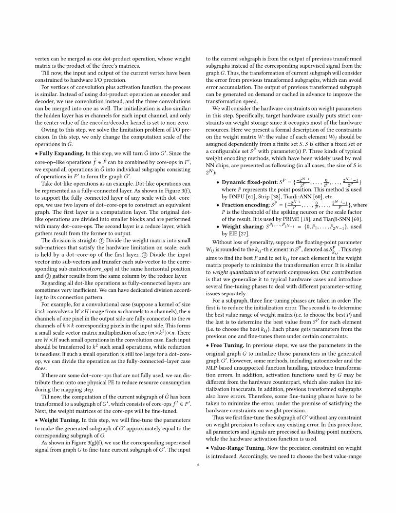
Quite a few NN applications, including an MLP for MNISTdataset (784-100-10 structure, 98.2% accuracy of full precision),LeNet-5 [42] for MNIST dataset (99.1% accuracy), a CNN [53] forCIFAR-10 dataset (84.64% accuracy 1), AlexNet [41] and VGG16 [62]for ImageNet, have been respectively transformed and then de-ployed onto TianJi [60] and PRIME [18] to show the validation. The

1As described by [53], with some special initialization method, the CNN accuracy canexceed 90%. Here we ignore it for simplicity, which does not affect our evaluation.

7

NN model Chip Weight Encoding Weight I/O Re-encoding Top1 AccuracyPrecision Precision Factor (Accuracy Drop)

MNIST-MLP Floating-point 98.2%MNIST-MLP TianJi-ANN Dynamic fixed-point 8-bit 8-bit 1× 98.15%(-0.05%)MNIST-MLP TianJi-SNN Fraction encoding 8-bit 1-bit 2× 96.59%(-1.61%)MNIST-MLP TianJi-SNN Fraction encoding 8-bit 2-bit 2× 97.63%(-0.57%)MNIST-MLP PRIME Fraction encoding 8-bit 6-bit 1× 98.14%(-0.06%)LetNet-5 Floating-point 99.1%LeNet-5 TianJi-ANN Dynamic fixed-point 8-bit 8-bit 1× 99.08%(-0.02%)LeNet-5 PRIME Fraction encoding 8-bit 6-bit 1× 99.01%(-0.09%)CIFAR10-VGG17 Floating-point 84.64%CIFAR10-VGG17 TianJi-ANN Dynamic fixed-point 8-bit 8-bit 1× 84.02%(-0.62%)CIFAR10-VGG17 PRIME Fraction encoding 8-bit 6-bit 1× 83.57%(-1.07%)ImageNet-AlexNet Floating-point 57.4%ImageNet-AlexNet TianJi-ANN Dynamic fixed-point 8-bit 8-bit 1× 56.9%(-0.5%)ImageNet-AlexNet PRIME Fraction encoding 8-bit 6-bit 1× 55.2%(-2.2%)ImageNet-AlexNet PRIME Fraction encoding 8-bit 6-bit 4× 57.0%(-0.4%)ImageNet-VGG16 Floating-pint 70.5%ImageNet-VGG16 TianJi-ANN Dynamic fixed-point 8-bit 8-bit 1× 69.6%(-0.9%)ImageNet-VGG16 PRIME Fraction encoding 8-bit 6-bit 1× 68.2%(-2.3%)ImageNet-VGG16 PRIME Fraction encoding 8-bit 6-bit 4× 69.5%(-1.0%)

Table 2: Accuracy for NNs under different restrictions

first three networks are trained by Theano [4]. Parameters of thenext two CNNs for ImageNet are extracted from trained modelsof the Caffe Model Zoo directly. The inference accuracies of fullprecision are given in Table 2.

Without loss of generality, we take the mapping of the LeNet-5for MNIST onto the TianJi system as an example.

One TianJi chip contains 6 cores connected by a 2× 3mesh NoC;each core supports 256 simplified LIF neurons and works in theweight stationary mode. The main body of a TianJi system is aPrinted Circuit Board (PCB) including 16 chips. On the whole, all ofthe cores form a 12 × 8 2D-mesh network, and there is a great gapbetween the delay/bandwidth of intra-/inter-chip communications.

The transformed CG consists of 497 TianJi’s dot–core-op. Takinginto account the weight reuse of convolution, 19 physical coresare actually occupied. We use the heuristic Kernighan-Lin (KL)partitioning algorithm for the mapping problem. It abstracts themapping as a graph partition problem and tries to minimize com-munications across partition boundaries. Take the bipartition asan example: the input to the algorithm is a graph; the weight ofeach edge is the communication delay. The goal is to partition thegraph into two disjoint subset A and B of equal size, in a way thatminimizes the communication cost of the subset of edges that crossfrom A to B.

First, a randomly generated initial mapping distribution is given.Second,the KL algorithm bi-partitions the mapped cores repeatedly till onlythe closest two cores are left in any of the final partition in the2D-mesh. During this phase, partitions that minimize the commu-nication cost between cores are remained; here the cost of an edgeacross boundary refers to its weight multiplied by the number oftransmissions, as we can get the communication statistics from

the transformed CG, including those information about the reusedcores.

5.2 EvaluationThe inference accuracies after transformation for TianJi and PRIMEare given in Table 2. This table also shows the re-encoding factor,which indicate the number of hidden units for autoencoders, foreach case.

We can see that the transformation errors introduced are verylimited, for all NN models and chips tested, we can achieve lessthan 2% accuracy drop. For most cases, we only use 1× hidden unitto re-encode data, which means that the NN scale is not changed.For the two TianJi-SNN cases, as the I/O constraints are very strict,we use 2× hidden units, thus 4× PEs will be used. For ImageNetcases on PRIME, if we only use 1× hidden units, the accuracy dropwill be over 2%. With 4× hidden units, we can reduce the accuracydrop to less than 1%. We can always achieve better accuracy withmore hardware resources employed.

This toolchain also improves the development efficiency remark-ably. For example, it can transform AlexNet in about 1 hour, whiletraining it from scratch will take about 3~4 days. Specially, trainingthe whole NN requires millions of iterations to converge, while ourmethod only costs thousands of iterations to converge for each step,that is, takes 5 to 10 minutes to transform one layer. The reason liesin that, after partitioning, we fine-tune each unit one by one; eachone is well initialized and much easier to converge than trainingthe entire model. All evaluations are completed on a common PCserver equipped with one Tesla P100 GPU.

In addition, as the large-scale NNs (e.g. those for ImageNet)cannot be occupied by the TianJi system because of the physicallimit of chip capacity (a TianJi system contains 16 chips and a chip

8

75.00%

80.00%

85.00%

90.00%

95.00%

100.00%

1 2 3 4 5

Acc

ura

cy(R

elat

ive

to g

old

en m

od

el)

I/O precision (bits)

without autoencoder 1× hidden nodes2× hidden nodes 3× hidden nodes4× hidden nodes

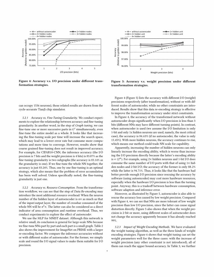
Figure 4: Accuracy v.s. I/O precision under different trans-formation strategies.

can occupy 1536 neurons), those related results are drawn from thecycle-accurate TianJi chip simulator.

5.2.1 Accuracy vs. Fine-Tuning Granularity. We conduct experi-ments to explore the relationship between accuracy and fine-tuninggranularity. In another word, in the step of Graph tuning, we canfine-tune one or more successive parts in G ′ simultaneously, evenfine-tune the entire model as a whole. It looks like that increas-ing the fine-tuning scale per time will increase the search space,which may lead to a lower error rate but consume more compu-tations and more time to converge. However, results show thatcoarse grained fine-tuning does not result in improved accuracy.For example, for CIFAR10-CNN, the inference accuracy (the I/Oprecision is 7 bits and the weight precision is 4 bits) is 83.07% as thefine-tuning-granularity is two subgraphs (the accuracy is 83.14% asthe granularity is one). If we fine-tune the whole NN together, theaccuracy is just 83.24%. Thus, one by one fine-tuning is an optimalstrategy, which also means that the problem of error accumulationhas been well solved. Unless specifically noted, the fine-tuninggranularity is just one.

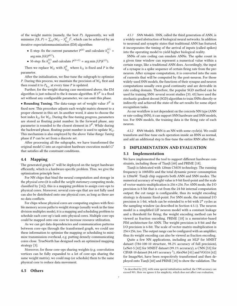
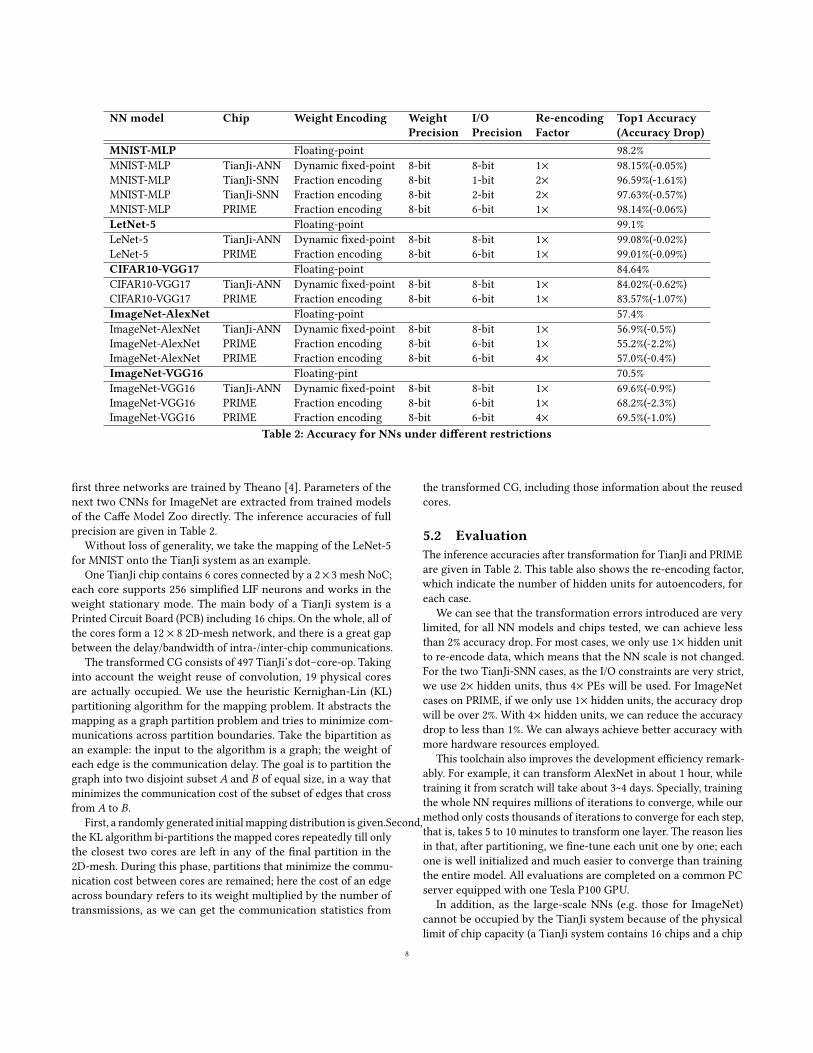
5.2.2 Accuracy vs. Resource Consumption. From the transforma-tion workflow, we can see that the step of Data Re-encoding mayintroduce the most additional resource overhead: When the neuronnumber of the hidden layer of autoencoder is n× as much as thatof the input/output layer, the number of crossbar consumed of thewhole NN will be n2×. The latter can also be considered as a directindicator of area consumption and runtime overhead. Thus, weconduct experiments to explore the effect of autoencoder.

We use the MLP for MNIST dataset. Although this network isrelative small, its conclusion is general for large-scale NNs becausewe fine-tune NNs part by part and each part is a small graph. Table 2also shows the improvement for ImageNet on PRIME with a largerre-encoding factor. We compare the inference accuracies withoutor with different scales of autoencoder. For the former, we simplyscale and round the I/O signal values to make them suitable for I/Oprecision.

96.00%

97.00%

98.00%

99.00%

100.00%

2 3 4

Acc

ura

cy(R

elat

ive

to g

old

en m

od

el)

Weight precision (bits)

without autoencoder 1× hidden unit2× hidden unit 3× hidden unit4× hidden unit

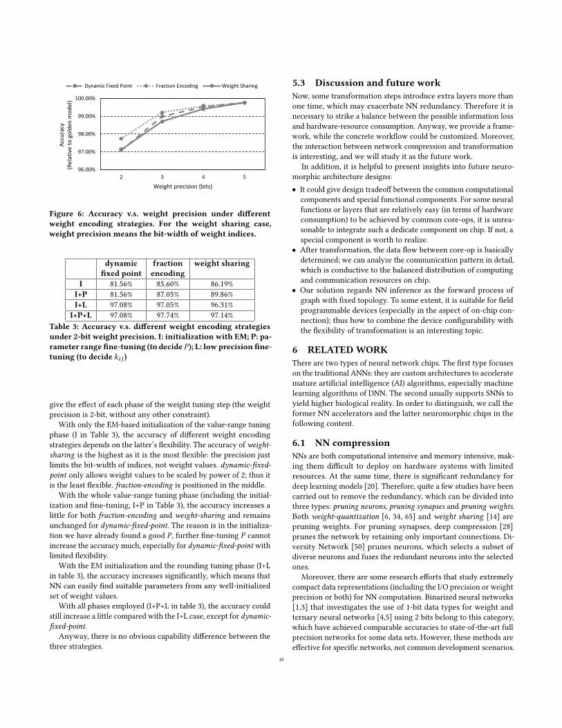
Figure 5: Accuracy v.s. weight precision under differenttransformation strategies.

Figure 4 (Figure 5) lists the accuracy with different I/O (weight)precisions respectively (after transformation), without or with dif-ferent scales of autoencoder, while no other constraints are intro-duced. Results show that this data re-encoding strategy is effectiveto improve the transformation accuracy under strict constraints.

In Figure 4, the accuracy of the transformed network withoutautoencoder drops significantly when I/O precision is less than 3bits (different NNs may have different turning points). In contrast,when autoencoder is used (we assume the I/O limitation is only1-bit and only 1x hidden neurons are used, namely, the most criticalcase), the accuracy is 84.63% (if no autoencoder, the value is only13.45%). With more hidden neurons, the accuracy continues to rise,which means our method could trade NN scale for capability.

Apparently, increasing the number of hidden neurons can onlylinearly increase the encoding ability, which is worse than increas-ing the I/O precision directly because the latter’s encoding abilityis ∝ (2n ). For example, using 2× hidden neurons and 1-bit I/O doesconsume the same number of I/O ports with that of using 1× hid-den nodes and 2-bit I/O; the accuracy of the former is only 88.2%while the latter is 94.71%. Thus, it looks like that the hardware hadbetter provide enough I/O precision since rescuing the accuracy bysoftware (using autoencoder) may cost more hardware resources,especially when the hardware I/O precision is less than the turningpoint. Anyway, this is a tradeoff between hardware consumption,software adaption and inference error.

Moreover, as illustrated by Figure 5, autoencoder is also able torescue the accuracy loss caused by low weight precision. Comparedwith Figure 4, we can see that NNs are more tolerant of low weightprecision than low I/O precision, since the latter can cause signaldistortion directly. Figure 5 also shows that when the weight pre-cision is 2-bit or more, using different scales of autoencoder doesnot change the accuracy apparently because it has already reached99%.

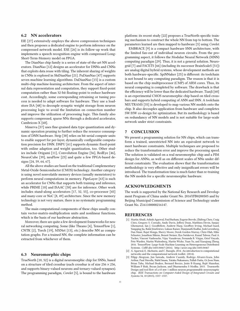
5.2.3 Impact of Weight Encoding Methods. We have evaluatedthe weight tuning algorithm, as well as the three kinds of weightencoding strategies. Figure 6 shows that weight tuning can set theweight parameters well for the three cases: with the increase ofweight precision (any other constraint is not introduced), all ofthem can reach the upper bound accuracy. In Table 3, we further

9

96.00%

97.00%

98.00%

99.00%

100.00%

2 3 4 5

Acc

ura

cy(R

elat

ive

to g

old

en m

od

el)

Weight precision (bits)

Dynamic Fixed Point Fraction Encoding Weight Sharing

Figure 6: Accuracy v.s. weight precision under differentweight encoding strategies. For the weight sharing case,weight precision means the bit-width of weight indices.

dynamic fraction weight sharingfixed point encoding

I 81.56% 85.60% 86.19%I+P 81.56% 87.05% 89.86%I+L 97.08% 97.05% 96.31%

I+P+L 97.08% 97.74% 97.14%Table 3: Accuracy v.s. different weight encoding strategiesunder 2-bit weight precision. I: initialization with EM; P: pa-rameter range fine-tuning (to decide P ); L: low precision fine-tuning (to decide ki j )

give the effect of each phase of the weight tuning step (the weightprecision is 2-bit, without any other constraint).

With only the EM-based initialization of the value-range tuningphase (I in Table 3), the accuracy of different weight encodingstrategies depends on the latter’s flexibility. The accuracy of weight-sharing is the highest as it is the most flexible: the precision justlimits the bit-width of indices, not weight values. dynamic-fixed-point only allows weight values to be scaled by power of 2; thus itis the least flexible. fraction-encoding is positioned in the middle.

With the whole value-range tuning phase (including the initial-ization and fine-tuning, I+P in Table 3), the accuracy increases alittle for both fraction-encoding and weight-sharing and remainsunchanged for dynamic-fixed-point. The reason is in the initializa-tion we have already found a good P , further fine-tuning P cannotincrease the accuracy much, especially for dynamic-fixed-point withlimited flexibility.

With the EM initialization and the rounding tuning phase (I+Lin table 3), the accuracy increases significantly, which means thatNN can easily find suitable parameters from any well-initializedset of weight values.

With all phases employed (I+P+L in table 3), the accuracy couldstill increase a little compared with the I+L case, except for dynamic-fixed-point.

Anyway, there is no obvious capability difference between thethree strategies.

5.3 Discussion and future workNow, some transformation steps introduce extra layers more thanone time, which may exacerbate NN redundancy. Therefore it isnecessary to strike a balance between the possible information lossand hardware-resource consumption. Anyway, we provide a frame-work, while the concrete workflow could be customized. Moreover,the interaction between network compression and transformationis interesting, and we will study it as the future work.

In addition, it is helpful to present insights into future neuro-morphic architecture designs:• It could give design tradeoff between the common computational

components and special functional components. For some neuralfunctions or layers that are relatively easy (in terms of hardwareconsumption) to be achieved by common core-ops, it is unrea-sonable to integrate such a dedicate component on chip. If not, aspecial component is worth to realize.

• After transformation, the data flow between core-op is basicallydetermined; we can analyze the communication pattern in detail,which is conductive to the balanced distribution of computingand communication resources on chip.

• Our solution regards NN inference as the forward process ofgraph with fixed topology. To some extent, it is suitable for fieldprogrammable devices (especially in the aspect of on-chip con-nection); thus how to combine the device configurability withthe flexibility of transformation is an interesting topic.

6 RELATEDWORKThere are two types of neural network chips. The first type focuseson the traditional ANNs: they are custom architectures to acceleratemature artificial intelligence (AI) algorithms, especially machinelearning algorithms of DNN. The second usually supports SNNs toyield higher biological reality. In order to distinguish, we call theformer NN accelerators and the latter neuromorphic chips in thefollowing content.

6.1 NN compressionNNs are both computational intensive and memory intensive, mak-ing them difficult to deploy on hardware systems with limitedresources. At the same time, there is significant redundancy fordeep learning models [20]. Therefore, quite a few studies have beencarried out to remove the redundancy, which can be divided intothree types: pruning neurons, pruning synapses and pruning weights.Both weight-quantization [6, 34, 65] and weight sharing [14] arepruning weights. For pruning synapses, deep compression [28]prunes the network by retaining only important connections. Di-versity Network [50] prunes neurons, which selects a subset ofdiverse neurons and fuses the redundant neurons into the selectedones.

Moreover, there are some research efforts that study extremelycompact data representations (including the I/O precision or weightprecision or both) for NN computation. Binarized neural networks[1,3] that investigates the use of 1-bit data types for weight andternary neural networks [4,5] using 2 bits belong to this category,which have achieved comparable accuracies to state-of-the-art fullprecision networks for some data sets. However, these methods areeffective for specific networks, not common development scenarios.

10

6.2 NN acceleratorsEIE [27] extensively employs the above compression techniquesand then proposes a dedicated engine to perform inference on thecompressed network model. ESE [26] is its follow-up work thatimplements a speech recognition engine with compressed Long-Short-Term-Memory model on FPGA.

The DianNao chip family is a series of state-of-the-art NN accel-erators. DianNao [12] designs an accelerator for DNNs and CNNsthat exploits data reuse with tiling. The inherent sharing of weightsin CNNs is explored in ShiDianNao [21]. PuDianNao [47] supportsseven machine learning algorithms. DaDianNao [15] is a custommulti-chip machine-learning architecture. From the aspect of inter-nal data representation and computation, they support fixed-pointcomputation rather than 32-bit floating-point to reduce hardwarecost. Accordingly, some corresponding retraining or tuning pro-cess is needed to adapt software for hardware. They use a load-store ISA [48] to decouple synaptic weight storage from neuronprocessing logic to avoid the limitation on connection numberand improve the utilization of processing logic. This family alsosupports compressed, sparse NNs through a dedicated accelerator,Cambricon-X [68].

Minerva [57] uses fine-grained data type quantization and dy-namic operation pruning to further reduce the resource consump-tion of DNN hardware. Strip [38] relies on bit-serial compute unitsto enable support for per-layer, dynamically configurable computa-tion precision for DNN. DNPU [61] supports dynamic fixed-pointwith online adaption and weight quantization, too. Other stud-ies include Origami [11], Convolution Engine [56], RedEye [46],NeuroCube [39], neuFlow [23] and quite a few FPGA-based de-signs [24, 59, 64, 67].

All the above studies are based on the traditional ComplementaryMetal-Oxide-Semiconductor (CMOS) technology. Another categoryis using novel nonvolatile memory devices (usually memristors) toperform neural computations in memory. PipeLayer [63] is suchan accelerator for CNNs that supports both training and inference,while PRIME [18] and ISAAC [58] are for inference. Other workincludes stand-along accelerators [17, 32, 55], co-processor [45]and many-core or NoC [8, 49] architecture. Since the new memorytechnology is not very mature, there is no systematic programmingmethod.

The main computational components of these chips usually con-tain vector-matrix-multiplication units and nonlinear functions,which is the basis of our hardware abstraction.

Moreover, there are quite a few development frameworks for neu-ral networking computing. Some (like Theano [4], TensorFlow [1],CNTK [2], Torch [19], MXNet [13], etc.) describe NN as compu-tation graphs. For a trained NN, the complete information can beextracted from whichever of them.

6.3 Neuromorphic chipsTrueNorth [10, 52] is a digital neuromorphic chip for SNNs, basedon a structure of tiled crossbar (each crossbar is of size 256 × 256,and supports binary-valued neurons and ternary-valued synapses).The programming paradigm, Corelet [5], is bound to the hardware

platform: its recent study [22] proposes a TrueNorth-specific train-ing mechanism to construct the whole NN from top to bottom. Theparameters learned are then mapped to hardware [3] using Corelet.

EMBRACE [9] is a compact hardware SNN architecture, withthe limited fan-out of individual neuron circuits. From the pro-gramming aspect, it follows the Modular Neural Network (MNN)computing paradigm [29]. Thus, it is not a general solution. Neuro-grid [7] and FACETS [66] (including its successor BrainScaleS [51])are analog/digital hybrid systems, whose development methods areboth hardware-specific. SpiNNaker [25] is different: its toolchainis not bound to any computing paradigm. The reason is that it isbased on the chip multiprocessor (CMP) of ARM cores. Thus, itsneural computing is completed by software. The drawback is thatthe efficiency will be lower than the dedicated hardware. TianJi [60]is an experimental CMOS neuromorphic chip based on tiled cross-bars and supports hybrid computing of ANN and SNN. A toolchainNEUTRAMS [35] is developed to map various NN models onto thechip. It also decouples application from hardware and completesSW/HW co-design for optimization. But its methodology is basedon redundancy of NN models and is not suitable for large-scalenetwork under strict constraints.

7 CONCLUSIONWe present a programming solution for NN chips, which can trans-form a trained, unrestricted NN into an equivalent network tomeet hardware constraints. Multiple techniques are proposed toreduce the transformation error and improve the processing speed.The solution is validated on a real neuromorphic chip and a PIMdesign for ANNs, as well as on different scales of NNs under dif-ferent constraints. The evaluation shows that the transformationmethodology is very effective and only insignificant errors will beintroduced. The transformation time is much faster than re-trainingthe NN models for a specific neuromorphic hardware.

ACKNOWLEDGMENTSThe work is supported by the National Key Research and Develop-ment Program of China under Grant No. 2016YFB0200505 and byBeijing Municipal Commission of Science and Technology underGrant No. Z161100000216147.

REFERENCES[1] Martín Abadi, Ashish Agarwal, Paul Barham, Eugene Brevdo, Zhifeng Chen, Craig

Citro, Gregory S. Corrado, Andy Davis, Jeffrey Dean, Matthieu Devin, SanjayGhemawat, Ian J. Goodfellow, Andrew Harp, Geoffrey Irving, Michael Isard,Yangqing Jia, Rafal Józefowicz, Lukasz Kaiser, Manjunath Kudlur, Josh Levenberg,Dan Mané, Rajat Monga, Sherry Moore, Derek Gordon Murray, Chris Olah, MikeSchuster, Jonathon Shlens, Benoit Steiner, Ilya Sutskever, Kunal Talwar, Paul A.Tucker, Vincent Vanhoucke, Vijay Vasudevan, Fernanda B. Viégas, Oriol Vinyals,Pete Warden, Martin Wattenberg, Martin Wicke, Yuan Yu, and Xiaoqiang Zheng.2016. TensorFlow: Large-Scale Machine Learning on Heterogeneous DistributedSystems. CoRR abs/1603.04467 (2016). http://arxiv.org/abs/1603.04467

[2] A. Agarwal, E. Akchurin, and C. Basoglu. 2014. An introduction to computationalnetworks and the computational network toolkit. (2014).

[3] Filipp Akopyan, Jun Sawada, Andrew Cassidy, Rodrigo Alvarez-Icaza, JohnArthur, Paul Merolla, Nabil Imam, Yutaka Nakamura, Pallab Datta, Gi-Joon Nam,Brian Taba, Michael Beakes, Bernard Brezzo, Jente B Kuang, Rajit Manohar,William P Risk, Bryan Jackson, and Dharmendra S Modha. 2015. Truenorth:Design and tool flow of a 65 mw 1 million neuron programmable neurosynapticchip. IEEE Transactions on Computer-Aided Design of Integrated Circuits andSystems 34, 10 (2015), 1537–1557.

11

[4] Rami Al-Rfou, Guillaume Alain, Amjad Almahairi, Christof Angermüller, DzmitryBahdanau, Nicolas Ballas, Frédéric Bastien, Justin Bayer, Anatoly Belikov, Alexan-der Belopolsky, Yoshua Bengio, Arnaud Bergeron, James Bergstra, Valentin Bis-son, Josh Bleecher Snyder, Nicolas Bouchard, Nicolas Boulanger-Lewandowski,Xavier Bouthillier, Alexandre de Brébisson, Olivier Breuleux, Pierre Luc Car-rier, Kyunghyun Cho, Jan Chorowski, Paul Christiano, Tim Cooijmans, Marc-Alexandre Côté, Myriam Côté, Aaron C. Courville, Yann N. Dauphin, OlivierDelalleau, Julien Demouth, Guillaume Desjardins, Sander Dieleman, LaurentDinh, Melanie Ducoffe, Vincent Dumoulin, Samira Ebrahimi Kahou, DumitruErhan, Ziye Fan, Orhan Firat, Mathieu Germain, Xavier Glorot, Ian J. Good-fellow, Matthew Graham, Çaglar Gülçehre, Philippe Hamel, Iban Harlouchet,Jean-Philippe Heng, Balázs Hidasi, Sina Honari, Arjun Jain, Sébastien Jean, KaiJia, Mikhail Korobov, Vivek Kulkarni, Alex Lamb, Pascal Lamblin, Eric Larsen,César Laurent, Sean Lee, Simon Lefrançois, Simon Lemieux, Nicholas Léonard,Zhouhan Lin, Jesse A. Livezey, Cory Lorenz, Jeremiah Lowin, Qianli Ma, Pierre-Antoine Manzagol, Olivier Mastropietro, Robert McGibbon, Roland Memisevic,Bart van Merriënboer, Vincent Michalski, Mehdi Mirza, Alberto Orlandi, Christo-pher Joseph Pal, Razvan Pascanu, Mohammad Pezeshki, Colin Raffel, DanielRenshaw, Matthew Rocklin, Adriana Romero, Markus Roth, Peter Sadowski,John Salvatier, François Savard, Jan Schlüter, John Schulman, Gabriel Schwartz,Iulian Vlad Serban, Dmitriy Serdyuk, Samira Shabanian, Étienne Simon, SigurdSpieckermann, S. Ramana Subramanyam, Jakub Sygnowski, Jérémie Tanguay,Gijs van Tulder, Joseph P. Turian, Sebastian Urban, Pascal Vincent, FrancescoVisin, Harm de Vries, David Warde-Farley, Dustin J. Webb, Matthew Willson,Kelvin Xu, Lijun Xue, Li Yao, Saizheng Zhang, and Ying Zhang. 2016. Theano:A Python framework for fast computation of mathematical expressions. CoRRabs/1605.02688 (2016). http://arxiv.org/abs/1605.02688

[5] Arnon Amir, Pallab Datta, William P Risk, Andrew S Cassidy, Jeffrey A Kusnitz,Steve K Esser, Alexander Andreopoulos, Theodore M Wong, Myron Flickner, Ro-drigo Alvarez-Icaza, Emmett McQuinn, Ben Shaw, Norm Pass, and Dharmendra SModha. 2013. Cognitive computing programming paradigm: a corelet languagefor composing networks of neurosynaptic cores. In Neural Networks (IJCNN),The 2013 International Joint Conference on. IEEE, 1–10.

[6] Sajid Anwar, Kyuyeon Hwang, and Wonyong Sung. 2015. Fixed point optimiza-tion of deep convolutional neural networks for object recognition. In Acoustics,Speech and Signal Processing (ICASSP), 2015 IEEE International Conference on.IEEE, 1131–1135.

[7] Ben Varkey Benjamin, Peiran Gao, Emmett McQuinn, Swadesh Choudhary,Anand R Chandrasekaran, Jean-Marie Bussat, Rodrigo Alvarez-Icaza, John VArthur, Paul A Merolla, and Kwabena Boahen. 2014. Neurogrid: A mixed-analog-digital multichip system for large-scale neural simulations. Proc. IEEE 102, 5(2014), 699–716.

[8] Mahdi Nazm Bojnordi and Engin Ipek. 2016. Memristive Boltzmann machine: Ahardware accelerator for combinatorial optimization and deep learning. In HighPerformance Computer Architecture (HPCA), 2016 IEEE International Symposiumon. 1–13.

[9] Snaider Carrillo, Jim Harkin, Liam J McDaid, Fearghal Morgan, Sandeep Pande,Seamus Cawley, and Brian McGinley. 2013. Scalable hierarchical network-on-chip architecture for spiking neural network hardware implementations. IEEETransactions on Parallel and Distributed Systems 24, 12 (2013), 2451–2461.

[10] Andrew S Cassidy, Paul Merolla, John V Arthur, Steve K Esser, Bryan Jackson,Rodrigo Alvarez-Icaza, Pallab Datta, Jun Sawada, Theodore M Wong, Vitaly Feld-man, Arnon Amir, Daniel Ben-Dayan Rubin, Filipp Akopyan, Emmett McQuinn,William P Risk, and Dharmendra S Modha. 2013. Cognitive computing buildingblock: A versatile and efficient digital neuron model for neurosynaptic cores. InNeural Networks (IJCNN), The 2013 International Joint Conference on. IEEE, 1–10.

[11] Lukas Cavigelli and Luca Benini. 2016. A 803 gop/s/w convolutional networkaccelerator. IEEE Transactions on Circuits and Systems for Video Technology (2016).

[12] Tianshi Chen, Zidong Du, Ninghui Sun, Jia Wang, Chengyong Wu, Yunji Chen,and Olivier Temam. 2014. Diannao: A small-footprint high-throughput accel-erator for ubiquitous machine-learning. In ACM Sigplan Notices, Vol. 49. ACM,269–284.

[13] Tianqi Chen, Mu Li, Yutian Li, Min Lin, Naiyan Wang, Minjie Wang, TianjunXiao, Bing Xu, Chiyuan Zhang, and Zheng Zhang. 2015. Mxnet: A flexible andefficient machine learning library for heterogeneous distributed systems. arXivpreprint arXiv:1512.01274.

[14] Wenlin Chen, James Wilson, Stephen Tyree, Kilian Weinberger, and Yixin Chen.2015. Compressing neural networks with the hashing trick. In InternationalConference on Machine Learning. 2285–2294.

[15] Yunji Chen, Tao Luo, Shaoli Liu, Shijin Zhang, Liqiang He, Jia Wang, Ling Li,Tianshi Chen, Zhiwei Xu, Ninghui Sun, and Olivier Teman. 2014. Dadiannao: Amachine-learning supercomputer. In Proceedings of the 47th Annual IEEE/ACMInternational Symposium on Microarchitecture. IEEE Computer Society, 609–622.

[16] Y. H. Chen, T. Krishna, J. Emer, and V. Sze. 2016. 14.5 Eyeriss: An energy-efficient reconfigurable accelerator for deep convolutional neural networks. In2016 IEEE International Solid-State Circuits Conference (ISSCC). 262–263. https://doi.org/10.1109/ISSCC.2016.7418007

[17] Zhen Chen, Bin Gao, Zheng Zhou, Peng Huang, Haitong Li, and Wenjia Ma.2015. Optimized learning scheme for grayscale image recognition in a RRAM

based analog neuromorphic system. In Electron Devices Meeting (IEDM), 2015IEEE International. IEEE.

[18] Ping Chi, Shuangchen Li, Cong Xu, Tao Zhang, Jishen Zhao, Yongpan Liu, YuWang, and Yuan Xie. 2016. Prime: A novel processing-in-memory architecturefor neural network computation in reram-based main memory. In Proceedings ofthe 43rd International Symposium on Computer Architecture. IEEE Press, 27–39.

[19] Ronan Collobert, Koray Kavukcuoglu, and Clement Farabet. 2011. Torch7: AMatlab-like Environment for Machine Learning. In neural information processingsystems.

[20] Misha Denil, Babak Shakibi, Laurent Dinh, Marc' Aurelio Ranzato, and Nandode Freitas. 2013. Predicting Parameters in Deep Learning. In Advances in Neu-ral Information Processing Systems 26, C. J. C. Burges, L. Bottou, M. Welling,Z. Ghahramani, and K. Q. Weinberger (Eds.). Curran Associates, Inc., 2148–2156.

[21] Zidong Du, Robert Fasthuber, Tianshi Chen, Paolo Ienne, Ling Li, Tao Luo,Xiaobing Feng, Yunji Chen, and Olivier Temam. 2015. ShiDianNao: Shiftingvision processing closer to the sensor. In ACM SIGARCH Computer ArchitectureNews, Vol. 43. ACM, 92–104.

[22] Steven K Esser, Paul A Merolla, John V Arthur, Andrew S Cassidy, Rathinaku-mar Appuswamy, Alexander Andreopoulos, David J Berg, Jeffrey L McKinstry,Timothy Melano, Davis R Barch, Carmelo di Nolfo, Pallab Datta, Arnon Amir,Brian Taba, Myron D Flickner, and Dharmendra S Modha. 2016. Convolutionalnetworks for fast, energy-efficient neuromorphic computing. Proceedings of theNational Academy of Sciences (2016), 201604850.

[23] Clément Farabet, Berin Martini, Benoit Corda, Polina Akselrod, Eugenio Cu-lurciello, and Yann LeCun. 2011. Neuflow: A runtime reconfigurable dataflowprocessor for vision. In Computer Vision and Pattern Recognition Workshops(CVPRW), 2011 IEEE Computer Society Conference on. IEEE, 109–116.

[24] Clément Farabet, Cyril Poulet, Jefferson Y Han, and Yann LeCun. 2009. Cnp: Anfpga-based processor for convolutional networks. In Field Programmable Logicand Applications, 2009. FPL 2009. International Conference on. IEEE, 32–37.

[25] Steve B Furber, David R Lester, Luis A Plana, Jim D Garside, Eustace Painkras,Steve Temple, and Andrew D Brown. 2013. Overview of the spinnaker systemarchitecture. IEEE Trans. Comput. 62, 12 (2013), 2454–2467.

[26] Song Han, Junlong Kang, Huizi Mao, Yiming Hu, Xin Li, Yubin Li, Dongliang Xie,Hong Luo, Song Yao, Yu Wang, Huazhong Yang, and William J. Dally. 2016. ESE:Efficient Speech Recognition Engine with Compressed LSTM on FPGA. CoRRabs/1612.00694 (2016). http://arxiv.org/abs/1612.00694

[27] Song Han, Xingyu Liu, Huizi Mao, Jing Pu, Ardavan Pedram, Mark A Horowitz,and William J Dally. 2016. EIE: efficient inference engine on compressed deepneural network. In Proceedings of the 43rd International Symposium on ComputerArchitecture. IEEE Press, 243–254.

[28] Song Han, Huizi Mao, andWilliam J Dally. 2015. Deep compression: Compressingdeep neural networks with pruning, trained quantization and huffman coding.arXiv preprint arXiv:1510.00149 (2015).

[29] Bart LM Happel and Jacob MJ Murre. 1994. Design and evolution of modularneural network architectures. Neural networks 7, 6 (1994), 985–1004.

[30] Kurt Hornik, Maxwell Stinchcombe, and Halbert White. 1989. Multilayer feed-forward networks are universal approximators. Neural networks 2, 5 (1989),359–366.

[31] Miao Hu, Hai Li, Yiran Chen, Qing Wu, and Garrett S Rose. 2013. BSB trainingscheme implementation onmemristor-based circuit. In Computational Intelligencefor Security and Defense Applications (CISDA), 2013 IEEE Symposium on. IEEE,80–87.

[32] Miao Hu, John Paul Strachan, Zhiyong Li, Emmanuelle M Grafals, NoraicaDavila, Catherine Graves, Sity Lam, Ning Ge, Jianhua Joshua Yang, and R StanleyWilliams. 2016. Dot-product engine for neuromorphic computing: programming1T1M crossbar to accelerate matrix-vector multiplication. In Design AutomationConference (DAC), 2016 53nd ACM/EDAC/IEEE. IEEE, 1–6.

[33] Eric Hunsberger and Chris Eliasmith. 2016. Training Spiking Deep Networksfor Neuromorphic Hardware. CoRR abs/1611.05141 (2016). http://arxiv.org/abs/1611.05141

[34] Kyuyeon Hwang and Wonyong Sung. 2014. Fixed-point feedforward deep neuralnetwork design using weights+ 1, 0, and- 1. In Signal Processing Systems (SiPS),2014 IEEE Workshop on. IEEE, 1–6.

[35] YU Ji, Youhui Zhang, ShuangChen Li, Ping Chi, CiHang Jiang, Peng Qu, YuanXie, and WenGuang Chen. 2016. NEUTRAMS: Neural Network Transformationand Co-design under Neuromorphic Hardware Constraints. In Microarchitecture(MICRO), 2016 49th Annual IEEE/ACM International Symposium on.

[36] Yangqing Jia, Evan Shelhamer, Jeff Donahue, Sergey Karayev, Jonathan Long,Ross Girshick, Sergio Guadarrama, and Trevor Darrell. 2014. Caffe: Convolu-tional architecture for fast feature embedding. In Proceedings of the 22nd ACMinternational conference on Multimedia. ACM, 675–678.

[37] Norman P. Jouppi, Cliff Young, Nishant Patil, David Patterson, Gaurav Agrawal,Raminder Bajwa, Sarah Bates, Suresh Bhatia, Nan Boden, Al Borchers, Rick Boyle,Pierre-luc Cantin, Clifford Chao, Chris Clark, Jeremy Coriell, Mike Daley, MattDau, Jeffrey Dean, Ben Gelb, Tara Vazir Ghaemmaghami, Rajendra Gottipati,William Gulland, Robert Hagmann, Richard C. Ho, Doug Hogberg, John Hu,

12

Robert Hundt, Dan Hurt, Julian Ibarz, Aaron Jaffey, Alek Jaworski, AlexanderKaplan, Harshit Khaitan, Andy Koch, Naveen Kumar, Steve Lacy, James Laudon,James Law, Diemthu Le, Chris Leary, Zhuyuan Liu, Kyle Lucke, Alan Lundin,GordonMacKean, AdrianaMaggiore, MaireMahony, KieranMiller, Rahul Nagara-jan, Ravi Narayanaswami, Ray Ni, Kathy Nix, Thomas Norrie, Mark Omernick,Narayana Penukonda, Andy Phelps, Jonathan Ross, Amir Salek, Emad Samadiani,Chris Severn, Gregory Sizikov, Matthew Snelham, Jed Souter, Dan Steinberg,Andy Swing, Mercedes Tan, Gregory Thorson, Bo Tian, Horia Toma, Erick Tuttle,Vijay Vasudevan, Richard Walter, Walter Wang, Eric Wilcox, and Doe Hyun Yoon.2017. In-Datacenter Performance Analysis of a Tensor Processing Unit. CoRRabs/1704.04760. http://arxiv.org/abs/1704.04760

[38] Patrick Judd, Jorge Albericio, Tayler Hetherington, Tor M Aamodt, and AndreasMoshovos. 2016. Stripes: Bit-serial deep neural network computing. In Microar-chitecture (MICRO), 2016 49th Annual IEEE/ACM International Symposium on.IEEE, 1–12.

[39] Duckhwan Kim, Jaeha Kung, Sek Chai, Sudhakar Yalamanchili, and SaibalMukhopadhyay. 2016. Neurocube: A programmable digital neuromorphic ar-chitecture with high-density 3D memory. In Computer Architecture (ISCA), 2016ACM/IEEE 43rd Annual International Symposium on. IEEE, 380–392.

[40] Yongtae Kim, Yong Zhang, and Peng Li. 2015. A Reconfigurable Digital Neu-romorphic Processor with Memristive Synaptic Crossbar for Cognitive Com-puting. J. Emerg. Technol. Comput. Syst. 11, 4, Article 38 (April 2015), 25 pages.https://doi.org/10.1145/2700234

[41] Alex Krizhevsky, Ilya Sutskever, and Geoffrey E Hinton. 2012. ImageNet Clas-sification with Deep Convolutional Neural Networks. In Advances in NeuralInformation Processing Systems 25, F. Pereira, C. J. C. Burges, L. Bottou, and K. Q.Weinberger (Eds.). Curran Associates, Inc., 1097–1105.

[42] Yann LeCun, Léon Bottou, Yoshua Bengio, and Patrick Haffner. 1998. Gradient-based learning applied to document recognition. Proc. IEEE 86, 11 (1998), 2278–2324.

[43] Jun Haeng Lee, Tobi Delbruck, and Michael Pfeiffer. 2016. Training deep spikingneural networks using backpropagation. Frontiers in Neuroscience 10 (2016).

[44] Boxun Li, Yi Shan, Miao Hu, Yu Wang, Yiran Chen, and Huazhong Yang. 2013.Memristor-based approximated computation. In Proceedings of the 2013 Interna-tional Symposium on Low Power Electronics and Design. IEEE Press, 242–247.

[45] Boxun Li, Yi Shan, Miao Hu, Yu Wang, Yiran Chen, and Huazhong Yang. 2013.Memristor-based approximated computation. In international symposium on lowpower electronics and design. 242–247.

[46] Robert LiKamWa, Yunhui Hou, Julian Gao, Mia Polansky, and Lin Zhong. 2016.RedEye: analog ConvNet image sensor architecture for continuous mobile vision.In Proceedings of the 43rd International Symposium on Computer Architecture.IEEE Press, 255–266.

[47] Daofu Liu, Tianshi Chen, Shaoli Liu, Jinhong Zhou, Shengyuan Zhou, OlivierTeman, Xiaobing Feng, Xuehai Zhou, and Yunji Chen. 2015. Pudiannao: Apolyvalent machine learning accelerator. InACM SIGARCHComputer ArchitectureNews, Vol. 43. ACM, 369–381.

[48] Shaoli Liu, Zidong Du, Jinhua Tao, Dong Han, Tao Luo, Yuan Xie, Yunji Chen,and Tianshi Chen. 2016. Cambricon: An instruction set architecture for neu-ral networks. In Proceedings of the 43rd International Symposium on ComputerArchitecture. IEEE Press, 393–405.

[49] Xiaoxiao Liu, Mengjie Mao, Beiye Liu, Hai Li, Yiran Chen, Boxun Li, Yu Wang,Hao Jiang, Mark Barnell, Qing Wu, and Jianhua Yang. 2015. RENO: A high-efficient reconfigurable neuromorphic computing accelerator design. In DesignAutomation Conference (DAC), 2015 52nd ACM/EDAC/IEEE. IEEE, 1–6.

[50] Zelda Mariet and Suvrit Sra. 2015. Diversity Networks. CoRR abs/1511.05077(2015). http://arxiv.org/abs/1511.05077

[51] KarlheinzMeier. 2015. Amixed-signal universal neuromorphic computing system.In Electron Devices Meeting (IEDM), 2015 IEEE International. IEEE, 4–6.

[52] Paul A Merolla, John V Arthur, Rodrigo Alvarez-Icaza, Andrew S Cassidy, JunSawada, Filipp Akopyan, Bryan L Jackson, Nabil Imam, Chen Guo, Yutaka Naka-mura, Bernard Brezzo, lvan Vo, Steven K Esser, Rathinakumar Appuswamy,Brian Taba, Arnon Amir, Myron D Flickner, William P Risk, Rajit Manohar, and

Dharmendra S Modha. 2014. A million spiking-neuron integrated circuit with ascalable communication network and interface. Science 345, 6197 (2014), 668–673.

[53] Dmytro Mishkin and Jiri Matas. 2015. All you need is a good init. arXiv preprintarXiv:1511.06422 (2015).

[54] Vinod Nair and Geoffrey E Hinton. 2010. Rectified linear units improve re-stricted boltzmann machines. In Proceedings of the 27th international conferenceon machine learning (ICML-10). 807–814.

[55] Mirko Prezioso, Farnood Merrikh-Bayat, BD Hoskins, GC Adam, Konstantin KLikharev, and Dmitri B Strukov. 2015. Training and operation of an integratedneuromorphic network based on metal-oxide memristors. Nature 521, 7550 (2015),61–64.

[56] Wajahat Qadeer, Rehan Hameed, Ofer Shacham, Preethi Venkatesan, ChristosKozyrakis, and Mark A Horowitz. 2013. Convolution engine: balancing efficiency& flexibility in specialized computing. In ACM SIGARCH Computer ArchitectureNews, Vol. 41. ACM, 24–35.

[57] Brandon Reagen, Paul Whatmough, Robert Adolf, Saketh Rama, Hyunkwang Lee,Sae Kyu Lee, José Miguel Hernández-Lobato, Gu-Yeon Wei, and David Brooks.2016. Minerva: Enabling low-power, highly-accurate deep neural network acceler-ators. In Proceedings of the 43rd International Symposium on Computer Architecture.IEEE Press, 267–278.

[58] Ali Shafiee, Anirban Nag, Naveen Muralimanohar, Rajeev Balasubramonian,John Paul Strachan, Miao Hu, R Stanley Williams, and Vivek Srikumar. 2016.ISAAC: A convolutional neural network accelerator with in-situ analog arithmeticin crossbars. In Proceedings of the 43rd International Symposium on ComputerArchitecture. IEEE Press, 14–26.

[59] Hardik Sharma, Jongse Park, Divya Mahajan, Emmanuel Amaro, Joon KyungKim, Chenkai Shao, Asit Mishra, and Hadi Esmaeilzadeh. 2016. From high-leveldeep neural models to FPGAs. In Microarchitecture (MICRO), 2016 49th AnnualIEEE/ACM International Symposium on. IEEE, 1–12.

[60] L. Shi, J. Pei, N. Deng, D. Wang, L. Deng, Y. Wang, Y. Zhang, F. Chen, M. Zhao,S. Song, F. Zeng, G. Li, H. Li, and C. Ma. 2015. Development of a neuromorphiccomputing system. In 2015 IEEE International Electron Devices Meeting (IEDM).4.3.1–4.3.4. https://doi.org/10.1109/IEDM.2015.7409624

[61] Dongjoo Shin, Jinmook Lee, Jinsu Lee, and HoiJun Yoo. 2017. DNPU: An8.1TOPS/W Reconfigurable CNN-RNN Processor for General Purpose Deep Neu-ral Networks. In International Solid-State Circuits Conference. IEEE.

[62] Karen Simonyan and Andrew Zisserman. 2014. Very deep convolutional networksfor large-scale image recognition. arXiv preprint arXiv:1409.1556 (2014).

[63] Linghao Song, Xuehai Qian, Hai Li, and Yiran Chen. 2016. PipeLayer: A PipelinedReRAM-Based Accelerator for Deep Learning. In High Performance ComputerArchitecture (HPCA),2017 23rd IEEE Symposium on. IEEE.

[64] Lili Song, Ying Wang, Yinhe Han, Xin Zhao, Bosheng Liu, and Xiaowei Li. 2016.C-Brain: A deep learning accelerator that tames the diversity of CNNs throughadaptive data-level parallelization. In Design Automation Conference (DAC), 201653nd ACM/EDAC/IEEE. IEEE, 1–6.

[65] Vincent Vanhoucke, Andrew Senior, and Mark Z Mao. 2011. Improving the speedof neural networks on CPUs. In Proc. Deep Learning and Unsupervised FeatureLearning NIPS Workshop, Vol. 1. Citeseer, 4.

[66] Karsten Wendt, Matthias Ehrlich, and René Schüffny. 2008. A Graph Theo-retical Approach for a Multistep Mapping Software for the FACETS Project.In Proceedings of the 2Nd WSEAS International Conference on Computer En-gineering and Applications (CEA’08). World Scientific and Engineering Acad-emy and Society (WSEAS), Stevens Point, Wisconsin, USA, 189–194. http://dl.acm.org/citation.cfm?id=1373936.1373969

[67] Chen Zhang, Peng Li, Guangyu Sun, Yijin Guan, Bingjun Xiao, and Jason Cong.2015. Optimizing fpga-based accelerator design for deep convolutional neuralnetworks. In Proceedings of the 2015 ACM/SIGDA International Symposium onField-Programmable Gate Arrays. ACM, 161–170.

[68] Shijin Zhang, Zidong Du, Lei Zhang, Huiying Lan, Shaoli Liu, Ling Li, Qi Guo,Tianshi Chen, and Yunji Chen. 2016. Cambricon-X: An accelerator for sparseneural networks. In Microarchitecture (MICRO), 2016 49th Annual IEEE/ACMInternational Symposium on. IEEE, 1–12.

13