bridge & gp amp book

e-corder

®

www.

eDAQ

.com

eDAQ Amp User Manual

Bridge & GP Amp

Bridge Amp

GP Amp

ii Bridge & GP Amp

This document was, as far as possible, accurate at the time of printing. Changes may have been made to the software and hardware it describes since then: eDAQ Pty Ltd reserves the right to alter specifications as required. Late-breaking information may be supplied separately. Latest information and information and software updates can be obtained from our web site.

Trademarks of eDAQ

e-corder

and PowerChrom are registered trademarks of eDAQ Pty Ltd. Specific model names of data recording units, such as

e-corder

201, and PowerChrom 280, are trademarks of eDAQ Pty Ltd. Chart and Scope are trademarks of ADInstrumets Pty Ltd and are used under license by eDAQ. EChem is a trademarke of eDAQ Pty Ltd.

Other Trademarks

Mac OS, and Macintosh, are registered trademarks of Apple Computer, Inc. Windows 98, Windows Me, Windows 2000, and Windows XP are trademarks of Microsoft Corporation.

PostScript, and Acrobat are registered trademarks of Adobe Systems, Incorporated.

All other trademarks are the properties of their respective owners.

Products: Bridge Amp (EA110); GP Amp (EA142)

Document Number: U-EA110/EA142-1003

Copyright © October 2003

eDAQ Pty Ltd6 Doig AvenueDenistone East, NSW 2112AUSTRALIA

http://www.eDAQ.comemail: [email protected]

All rights reserved. No part of this document may be reproduced by any means without the prior written permission of eDAQ Pty Ltd.

Bridge

SeSeCoCoTe

3 T

The FInpTh

The BOI

2

C

Conten

1 Overview 1

How to Use this Manual 2eDAQ Amps 2Checking the Bridge or GP Amp 3

2 The Bridge Amp 5

The Front Panel 6Input Connector 6The Online Indicator 6

The Back Panel 7Output Connector 7I2C Connector 7

Connecting to the e-corder 8Using Chart & Scope Software 8

Previewing the signal 10Connecting Transducers 14

Wiring of the Transducer Plug 15

Bridge Amp

& GP Amp

tting Excitation Voltage 16tting the Offset Range 18nnecting Signal Leads 20nnecting the Excitation Leads 23sting the Transducer 23

he GP Amp 25

ront Panel 26ut Connector 26

e Online Indicator 26ack Panel 27utput Connector 27 Connector 27

ts

Connecting to the e-corder 28Using Chart & Scope Software 28

Previewing the signal 30Connecting Transducers 35

Wiring of Transducer Plug 35Setting Excitation Voltage 37Setting the Offset Range 39Connecting Signal Leads 41Connecting the Excitation Leads 42Testing the Transducer 42

A Technical Aspects 45

Overview 45Bridge Amp Construction 46GP Amp Construction 48

B Troubleshooting 51

iii

C Specifications 55

Bridge Amp 55GP Amp 57

Index 61

Licensing & Warranty 63

iv Bridge & GP Amp

Bridge

& GP Amp

1

C H A P T E R O N E

Overview

The Bridge Amp is designed for use with most full and half–bridge

transducers that require a differential DC amplifier providing high gain.

Typically these include force transducers, load cells, pressure

transducers, and similar devices.

The GP Amp is designed for use with powered transducers requiring

either a single–ended or differential high impedance (100 MΩ)

amplifier including piezoelectric devices, light meters, displacement

transducers and similar devices.

1

2

How to Use this Manual

This Manual describes how to set up and begin using your Bridge Amp (Chapter 2) or GP Amp (Chapter 3). Their use with Chart and Scope software is also described. The appendices provide technical information, and cover troubleshooting should you encounter a problem.

eDAQ Amps

The Bridge and GP Amps are part of a family of preamplifiers known as eDAQ Amps designed for use with your

e-corder

system.

The Bridge and GP Amps are designed to be operated under full software control and are automatically recognised by Chart or Scope software which control gain range, offset and filter settings.

The range of eDAQ Amps includes the:

• pH/mV Amp, suitable for connection of pH, ion selective, and potentiometric (ORP) electrodes

• Potentiostat, a three–electrode potentiostat that can be used for voltammetric and amperometric experiments. Gain ranges of 20 nA to 100 mA in 1:2:5 steps.

• Picostat, a high sensitivity three–electrode potentiostat suitable for use with carbon fibre and other microelectrodes. Current gain

Bridge & GP Amp

ranges of 10 pA to 100 nA in 1:2:5 steps.

• Bridge Amp, suitable for sensors requiring a low drift, high gain differential amplifier. Also provides DC excitation

• GP Amp, suitable for high output sensors requiring a high impedance single ended or differential amplifier. Also provides DC excitation.

See our web site at www.eDAQ.com for more information.

Chapter 1 — Overview

Checking the Bridge or GP Amp

Before you begin working with the Bridge or GP Amp, you should check:

• the contents of the box in which you received your eDAQ Amp against the packing list

• carefully for any sign of physical damage that might have occurred during transit.

If you find a problem, please contact your eDAQ representative immediately.

You should also become familiar with the basic features of your

e-corder

system, which are discussed in the

Chart and Scope Software Manuals

on the Installer CD.

3

4

Bridge & GP Amp

Bridge

& GP Amp

2

C H A P T E R T W O

The Bridge Amp

This chapter describes the Bridge Amp, how to connect it to your

e-corder, and how to ensure that it is working properly. Configuring

your system for one or more eDAQ Amps is also discussed, along with

how to use the Bridge Amp with Chart and Scope software. Details on

how to wire a suitable connector plug for the attachment of a

transducer, or other sensor, to the Bridge Amp are also covered.

5

6

Figure 2–2 Input connector pin assignments, as seen when looking at the front panel

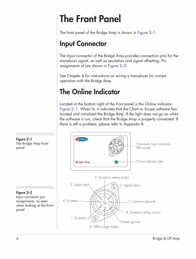
The Front Panel

The front panel of the Bridge Amp is shown in Figure 2–1.

Input Connector

The Input connector of the Bridge Amp provides connection pins for the transducer signal, as well as excitation and signal offsetting. Pin assignments of are shown in Figure 2–2.

See Chapter 4 for instructions on wiring a transducer for correct operation with the Bridge Amp.

The Online Indicator

Located at the bottom right of the front panel is the Online indicator, Figure 2–1. When lit, it indicates that the Chart or Scope software has located and initialised the Bridge Amp. If the light does not go on when the software is run, check that the Bridge Amp is properly connected. If there is still a problem, please refer to Appendix B.

Bridge Amp

Transducer input connectorDIN socket

Online indicator light

Figure 2–1 The Bridge Amp front panel

Bridge & GP Amp

7. Common (ground)

8. Excitation setting resistor

6. Offset range resistor

1. Excitation +

4. Excitation –

2. Signal input – 3. Signal input +


Chassis ground

Chapter 2 — The Bridge A

Figure 2–4 I2C connector pin assignments

The Back Panel

The back panel of the Bridge Amp is shown in Figure 2–3.

Output Connector

The Bridge Amp back panel, Figure 2–3, has a BNC connector labelled Analog Out. This is connected to an

e-corder

input channel. A suitable cable is included with the Bridge Amp.

I

2

C Connector

The Bridge Amp back panel, Figure 2–3, has two DB-9 pin ‘I

2

C bus’ connectors labelled Input and Output. The Input connector enables

Signal Output

Input OutputI CBusI C2

Signal output,BNC connector

I2C bus, DB-9 pin connectors

Figure 2–3 The Bridge Amp back panel

mp 7

1 5

96

Dig

ital G

roun

dRe

gula

ted

–17

V D

CRe

gula

ted

+8 V

DC

Regu

late

d +1

7 V

DC Power lines

SCL

DSC

SDA

DSD

INT

I2C control signals

15

9 6

Dig

ital G

roun

dRe

gula

ted

–17

V D

CRe

gula

ted

+8 V

DC

Regu

late

d +1

7 V

DC

SCL

DSC

SDA

DSD

INT

I2C control signals

Input Output

8

connection to the

e-corder

(or to the output of other eDAQ Amps). A cable is provided with the Bridge Amp for this purpose. This connection provides power to the Bridge Amp and carries the various control signals (for gain range and filter selection) to and from the e-corder. The pin assignments are shown in Figure 2–4.

The Output connector can be used to attach other eDAQ Amps.

More information about the I2C connector can be found in your e-corder Manual.

Connecting to the e-corderTo connect an eDAQ Amp, such as your Bridge Amp, to the e-corder, first make sure that the e-corder is turned off. Failure to do this may damage the e-corder, the Bridge Amp, or both.

Connect the I2C output of the e-corder to the I2C input of the Bridge Amp, using the cable provided, as shown in Figure 2–5. Check that the plugs for the cable are screwed in firmly. Connect the back panel Analog output of the Bridge Amp to one of the front panel input channels on the e-corder.

Check that all connections are firm. Loose connectors can cause the eDAQ Amp to fail to be recognised by the software, erratic behaviour, or loss of signal.

Multiple eDAQ Amps can be connected to a e-corder. The number that can be connected depends on the number of input channels on the

Bridge & GP Amp

e-corder. The initial eDAQ Amp should be connected as shown in Figure 2–5. The remainder are linked via I2C cables, connecting the I2C output of one eDAQ Amp to the I2C input of the next, as in Figure 2–6. The analog output of each eDAQ Amp is connected to one of the input channels of the e-corder.

Using Chart & Scope SoftwareWhen using the Chart or Scope data recording software with the Bridge Amp, the Input Amplifier dialog box that normally controls the e-corder input channel settings is replaced with the Bridge Amplifier dialog box. In this dialog box the separate amplification and filtering


Figure 2–6 Connecting multiple Bridges or other eDAQ Amps

settings for the Bridge Amp and e-corder are combined — that is you

I2C output I2C input

e-corder I2C output

I2C input

I2C connector cable

Signal output
Figure 2–5 Connecting a Bridge Amp to the e-corder
mp 9

see only one menu for amplification, and another menu for filter settings. The Chart and Scope Software Manuals (on the Installer CD) provide details the Input Amplifier dialog box.

The Bridge Amp Self-Test

Once the Bridge Amp is properly connected to the e-corder, and when the Chart and Scope software is installed on the computer, a quick check can be performed on the Bridge Amp:

• Turn on the e-corder and check that it is working properly, as described in the owner’s guide that was supplied with it.

10

• Once the e-corder is ready, open the Chart or Scope software. As the software opens, you should see the Bridge Amp indicator light, Figure 2–1, glow green, flash briefly, and then remain lit.

If the indicator glows green, the Bridge Amp is working properly. Otherwise it is not connected properly (re-check the connections) or that there is a software or hardware problem.

In addition when a Bridge Amp is properly connected to a channel, the usual e-corder Input Amplifier dialog box (see the e-corder Manual on the Installer CD) is replaced by the Bridge Amp dialog box, Figure 2–7 and Figure 2–8.

Previewing the signal

The Bridge Amplifier dialog box allows you to preview a signal so that you can select the amplification, filtering and other settings. The dialog boxes for Chart software are shown in Figure 2–7 and Figure 2–8. The Scope software controls are similar.

The incoming signal is displayed in real time, but is not recorded to hard disk (once the signal moves across the display area it is lost). Click the OK button to apply the selected settings. You are now ready to begin recording.

Signal Display

The input signal is previewed in real time — no data is being written to hard disk at this stage. Slowly changing waveforms will be represented

Bridge & GP Amp

quite accurately, whereas quickly changing signals will be displayed as a solid dark area showing only the envelope (shape) of the signal formed by the minimum and maximum recorded values. The average signal value is shown at the top left of the display area.

You can stop the signal scrolling by clicking the Pause button, . Click the Scroll button, , to start scrolling again. You can shift and stretch the vertical Amplitude axis to make the best use of the available display area (see the Input Amplifier dialog in the Chart Software Manual for further details). Changes made here update settings in the main window of the program.


Figure 2–7 The Bridge Amplifier dialog box, for previewing a signal. (Chart software on a Windows computer)

Figure 2–8 The Bridge Amplifier dialog box, for previewing a signal. (Chart software on a Macintosh)

e-corder input channel number Pause/Scroll button

Gain range

Select input channel

Filtering optionsAmplitude axis

e-corder input channel number Pause/Scroll buttons


External offset adjustment display

Units calibration Click the OK button to apply settings

Offset controls

Signal invert control

Gain range (sensitivity)

Incoming signal

Average signal amplitude


Offset display

mp 11

Filtering options

Amplitude axis


Units calibration

Offset controls

Incoming signal


(sensitivity)

Click the OK button to apply settings

Offset display

12

Setting the Range

The Range pop-up menu lets you select the input range or sensitivity of the channel — this is the total combined range of the e-corder and Bridge Amp. The default setting is 200 mV (the least sensitive range), but you can select from 12 ranges down to 50 µV (the most sensitive range). Within each range the resolution is 16 bits (Chart software) or 12 bits (Scope software).

Filtering

The High Pass and Low Pass pop-up menus provide signal filtering options appropriate to the type of transducer and quality of the signal recorded with the Bridge Amp.

High Pass. There are only two options: DC and 0.1 Hz. If DC is chosen then the high pass filter is turned off. When 0.1 Hz is chosen, high-pass filter (AC coupling) before the first amplification stage removes any DC and very low frequency components from the input. The 0.1 Hz option is sometimes useful to observe oscillating signals as it removes the baseline (DC) signal.

Low Pass. The Low Pass pop–up menu gives a choice of low-pass filters (1, 2, 10, 20, 100, 200 Hz, and 1 and 2 kHz) which can be used to remove high frequency (noise) components from the signal.

Inverting the Signal

Ticking the Invert checkbox inverts the direction of the signal. Positive

Bridge & GP Amp

signals are shown as negative values and vice versa.

For example, you might be recording from a force transducer where an increase in force downwards gives a negative signal, but you want to have a downwards force shown as a positive signal on the screen. Checking the Invert checkbox will change the display to do this.

Offset Adjustment

Even in the resting state most transducers still produce a non–zero signal. Zeroing, or offsetting, is the process by which this signal is set to a zero value. The offset controls in the Bridge Amplifier dialog box can


NOTE: Make sure that the transducer is recording a steady signal during the zeroing procedure. Changes in the transducer signal during the procedure could cause the auto-zeroing to fail.

be used to zero the reading manually or automatically. The total range of offset and the resolution of the offset controls are governed by the placement of a offset resistor across pins 6 and 7 in the transducer connector — see ‘Setting the Offset Range’, page 48, for more details.

Note that the zeroing features below are unavailable when the 0.1 Hz high pass filter (AC coupling) is selected, as this setting should remove DC offset component in the signal.

Manual Zeroing. The up and down arrow buttons next to the Zero button allow manual adjustment of signal zeroing. Click the up arrow to shift the signal positively, the down arrow to shift it negatively. The offset added by each click of the arrow buttons depends on the range setting.

Automatic Zeroing. To perform automatic zeroing, click the Zero button. Auto-zeroing may take 20 seconds or so to work out the best zeroing value at all ranges, but is a great deal quicker than manually going through each range. If there is still some offset after auto-zeroing, then Control+click (Option–click on Macintosh) the up and down arrow buttons to adjust the zeroing by small increments.

The offset display, a small numeric indicator above the Zero button, shows the offset used as a percentage value of the maximum offset available. When the Bridge Amp is first powered up, the software sets the offset circuit to no applied offset (its default position) and the offset display has a value of zero. When either the auto-zeroing function is selected or one the manual offset controls is used, this number will change to indicate the amount of offset applied.

mp 13

On Windows computers you can manually type in an offset value. A value of zero causes no offset to be applied.

On Macintosh click the button to restore the offset circuit to remove any applied offset (the offset display will return to zero).

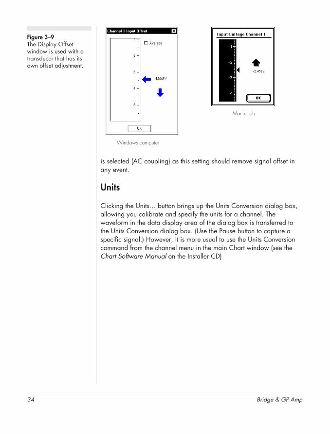
Display Offset

Clicking the Display Offset… button causes the Input Voltage dialog box to appear (Figure 2–9). If your transducer has its own offset adjustment capabilities, you can use this widow to help while zeroing the signal. This feature is unavailable when the 0.1 Hz high pass filter

14

Figure 2–9 The Display Offset window is used with a transducer that has its own offset adjustment.

is selected (AC coupling) as this setting should remove signal offset in any event.

Units

Clicking the Units… button brings up the Units Conversion dialog box, allowing you calibrate and specify the units for a channel. The waveform in the data display area of the dialog box is transferred to the Units Conversion dialog box. (Use the Pause button to capture a specific signal.) However, it is more usual to use the Units Conversion command from the channel menu in the main Chart window (see the Chart Software Manual on the Installer CD)

Windows computer

Macintosh

Bridge & GP Amp

Connecting TransducersThe Bridge Amp is designed to work with a wide variety of transducers and sensors that are configured as a DC Wheatstone bridge. These configurations require high gain, differential, low drift amplifiers. Differential signals up to 200 mV can be measured. Please refer to Appendix A (and especially Figure A–1 on page 47) for a technical description of this amplifier. This will assist you in the correct operation and wiring of the transducers used with the system.

The Bridge Amp is fitted with a female eight–pin DIN–style input socket to connect the transducer. A corresponding eight–pin DIN plug (male)


is also included. Additional eight–pin DIN plugs can be purchased from electronics suppliers, or from your eDAQ representative.

Wiring of the Transducer Plug

If you have purchased your transducer from eDAQ it will already have a suitable plug fitted. Otherwise, if you intend to use a transducer already fitted with a different connector you will have two options:

• Remove the existing connector and replace it with a compatible plug.

• assemble an adapter lead which allows the existing transducer to retain its original connector.

To wire a suitable plug for connection to the Bridge Amp you will need to perform the following actions:

1. Determine the required transducer excitation supply, select an appropriately sized Excitation Setting Resistor and fit this resistor between pins 5 and 8 of the DIN plug.

2. If a half–bridge transducer is being used, install appropriate half–bridge compensating resistors in the DIN plug.

3. Determine the required signal offset range, select an appropriate Offset Range Resistor and fit this resistor between pins 6 and 7of the DIN plug.

4. Identify the transducer signal leads and connect them to the appropriate pins of the DIN plug.

mp 15

5. Identify the transducer excitation (power) leads and connect them to the appropriate excitation supply on pins 1 and 4 of the DIN plug.

6. The main insulation sheath of the transducer cable should be clamped with the strain-relief device within the plug. Any unused wires from the transducer should be insulated to prevent shorting of signals or damage to the equipment.

The order of this procedure is important because any resistors used should be fitted before the signal and excitation leads are attached.

16

You will also need the following:

• a soldering iron and resin-cored solder (use only resin-cored solder) and some basic small electronic tools.

• a eight-pin DIN style male plug with 45° pin spacing (one is supplied with your Bridge or GP Amp)

• the connection diagram and specifications of the transducer you intend to use.

• a five–core shielded cable, if a cable is not already fitted to your transducer

• If you are using a half–bridge configuration, you will also need two 1000 Ω, 1%, 0.125 W high stability resistors. These resistors need to fit inside the plug body so small miniature types should be used.

While not difficult, it is recommended that this work should be done by a suitably qualified electronics technician with good soldering skills as incorrect wiring could damage the transducer and/or Bridge Amp. Such damage is not covered under the terms of your warranty.

There are several things to note when wiring connectors:

• Make sure that the transducer wiring is passed through the connector shell before soldering the wires to the plug.

• Wires should be cut, stripped, and tinned prior to soldering, to ensure a good connection.

• Use a small vice to hold the plug while soldering.

• The pin numbers shown in the diagrams are the numbers marked

Bridge & GP Amp

on standard DIN plugs. If the plug has no numbers or different ones, go by the layout shown in the Figures below.

Setting Excitation Voltage

Pins 1 and 4 of the input socket on the front panel of the Bridge Amp (and GP Amp) provide a DC excitation voltage from 0 V to 20 V (±10 V) to power the transducer. Pin 1 supplies up to +10 V, and pin 4 supplies down to –10 V with respect to ground, pin 7.


Figure 2–10 Placement of the Excitation Resistor in the transducer plug

The excitation voltage is set by connecting an Excitation Set Resistor between pins 5 and 8 on the DIN plug of the transducer. Correct mounting of the resistor is shown in Figure 2–10.

The relationship between the excitation voltage applied and the size of the resistor is given by:

where,

Rs = Excitation setting resistor in kΩ

Vex = Excitation voltage produced between pins 1 and 4 in volts

For example, the excitation voltage produced by a 330 kΩ resistor would be 6.25 V, or ±3.125 V, with respect to ground (pin 7).

Using this method will ensure that your transducer is automatically set to the correct excitation voltage when plugged into a Bridge or GP Amp.

1

2

3

4

5

6 7

8

Excitation resistor, Rs

Pin 5

Pin 8

Vex150

150 Rs+-------------------- 20×= …equation 2.1

mp 17

Special Cases

1. If there is no resistor across pins 5 and 8 (Rs = ∞) the value of Vex will be zero and your transducer will effectively be unpowered. This is a fail safe condition: if no excitation resistor is fitted then no excitation is generated.

2. Many transducers require ±5 V excitation. This is provided by using a 150 kΩ resistor.

18

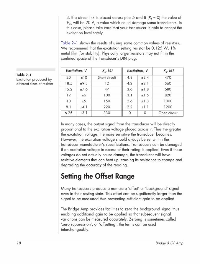
Table 2–1 Excitation produced by different sizes of resistor

3. If a direct link is placed across pins 5 and 8 (Rs = 0) the value of Vex will be 20 V, a value which could damage some transducers. In this case, please take care that your transducer is able to accept the excitation level safely.

Table 2–1 shows the results of using some common values of resistors. We recommend that the excitation setting resistor be 0.125 W, 1% metal film (for stability). Physically larger resistors may not fit in the confined space of the transducer’s DIN plug.

In many cases, the output signal from the transducer will be directly proportional to the excitation voltage placed across it. Thus the greater the excitation voltage, the more sensitive the transducer becomes. However, the excitation voltage should always be set within the transducer manufacturer’s specifications. Transducers can be damaged if an excitation voltage in excess of their rating is applied. Even if these voltages do not actually cause damage, the transducer will have resistive elements that can heat up, causing its resistance to change and degrading the accuracy of the reading.

Excitation, V Rs, kΩ Excitation, V Rs, kΩ

20 ±10 Short circuit 4.8 ±2.4 470

18.5 ±9.3 12 4.2 ±2.1 560

15.2 ±7.6 47 3.6 ±1.8 680

12 ±6 100 3.1 ±1.5 820

10 ±5 150 2.6 ±1.3 1000

8.1 ±4.1 220 2.2 ±1.1 1200

6.25 ±3.1 330 0 0 Open circuit

Bridge & GP Amp

Setting the Offset Range

Many transducers produce a non–zero ‘offset’ or ‘background’ signal even in their resting state. This offset can be significantly larger than the signal to be measured thus preventing sufficient gain to be applied.

The Bridge Amp provides facilities to zero the background signal thus enabling additional gain to be applied so that subsequent signal variations can be measured accurately. Zeroing is sometimes called ‘zero suppression’, or ‘offsetting’: the terms can be used interchangeably.


Figure 2–11 Placement of the Offset Range Resistor in the transducer plug (with excitation range resistor present)

You can zero the signal within the Chart or Scope software, Figure 2–7 and Figure 2–8. This is done by a circuit that uses a 12-bit DAC (digital–to–analog converter) to produce a voltage to zero the signal. The size of this voltage, Voff, is set by a Offset Range Resistor, the value of which, RB, is determined by procedures defined below.

The DAC can produce ±2048 steps within the offset range thus allowing very fine control of zeroing.

The maximum signal that you expect to obtain from your transducer is often a suitable offset range to select. For example a 1000 kg range force transducer (load cell) with a gain of 5 µV/V/kg, at an excitation of ±5 V, would be expected to output a 50 mV signal for a 1000 kg load. Thus if you need a 1000 kg offset you would need to set an offset range of 50 mV.

If you don’t know the gain of your transducer you first need to determine it by direct measurement of known values (for example for a load cell you would use one or more calibrated weights).

1

2

3

4

5

6 7

8

Excitation resistor, RsPin 7

Pin 6Offset range resistor, Roff

mp 19

The maximum offset available depends on the impedance of the bridge element of the transducer that you are using and the size of the offset range resistor is determined by:

where

Voff is the offset range available (V),

Roff is the size of the offset range resistor (kΩ), and

RB is the impedance of the transducer bridge element (kΩ)

V± off10 Roff+

110 Roff+--------------------------- RB×= …equation 2.2

20

Special cases

1. For RB = 300 Ω (a commonly encountered value) and Roff = 0 (short circuit across pins 6 and 7) the maximum offset is ±0.027 V, or 13 µV per step. This is very effective setting for many bridge transducers.

2. For RB =1000 ohms and Roff = ∞ (open circuit across pins 6 and 7) the maximum offset is ±0.91 V, or 444 µV per step.

By installing a resistor between pins 6 and 7 you can reduce the size of the DAC voltage steps and get increased resolution. However, the maximum offset available will be decreased correspondingly.

Decreasing values of resistance increase the resolution with which the signal can be zeroed, but decrease the maximum offset range available. Maximum resolution is obtained by short-circuiting the terminals (equivalent to using a zero ohm resistor).

In most cases an exact step size is not required and you should be able to use a resistor close to a value determined by the formula. It is recommend that you use a 1% metal film resistor rated at 0.125 W. Larger resistors may not fit in the confined space of the transducer’s DIN plug.

Once the required Offset Range resistance is calculated and a resistor is selected, it can be soldered between pins 6 and 7 of the DIN plug.

Connecting Signal Leads

Bridge & GP Amp

After the excitation and offset setting resistors have been fitted, the signal leads can now be connected. The general procedure is described below for both full and half–bridge type transducers.

The transducer cable will normally have a cable shield, which should be connected to pin 7 of the DIN plug. It is good practice to ensure that the shield is only connected to one ground point, either at the transducer or at the amplifier (but not both) otherwise ground loops will be set up leading to excessive noise.

If the casing of the plug is metal, it is good practice to ensure that the casing will also be connected to the shield.


Figure 2–12 Plug connections for a typical full–bridge transducer. The Offset Range resistor has been omitted.

The main insulation sheath of the transducer cable should be clamped with the strain-relief device within the plug. Any unused wires from the transducer should be insulated to prevent shorting of signals or damage to the equipment.

Full–Bridge transducers

Full-bridge transducers will have two signal leads ‘signal +’ and

1

2

3

4

5

67

8

Excitation voltage programming resistor

Ground or centre tap (shield)

Signal positive (+)

Signal negative (–)

Excitation negative (–)

Excitation positive (+)

��

Wire from transducer

Transducer ground (earth) wire

mp 21

‘signal –’ and often a ‘ground’ or ‘shield’ lead. These leads should be connected to pins 3, 2 and 7 respectively as shown in Figure 2–12.

Half–Bridge Transducers

A full–bridge arrangement is first made from the half–bridge transducer by adding two ‘half–bridge compensating’ resistors to the connector plug. One of these resistors links pin 1 and pin 2, while the second resistor links pin 4 and pin 2. Solder the resistors as shown in Figure 2–13. Notice that the top ends of the resistors are joined together and then soldered to pin 2.

22

Figure 2–13 Plug connections showing placement of half–bridge compensating resistors.

The value of these resistors should be equal to the nominal resistance of the active arms of the bridge, or 1 kΩ, whichever is the higher value.

Half–bridge compensating resistors

Pin 1

Pin 4

Pin 2

1�

2�

3�

4�

5�

6�7�

8�



Signal positive (+)


Excitation positive (+)

Half–bridge compensating resistors

Half–bridge compensating resistors should have the following specifications:Power rating: 0.25 or 0.125 W

Temperature coefficient: <10 ppm per °CMatched temperature coefficient: 1 ppm per °C

Resistor matching: <0.05%Resistor tolerance: ≤1%

Bridge & GP Amp

A change of 1 ppm in the relative values of the resistors will result in a change of 10 µV in the output for a 10 V excitation voltage. To avoid self-heating effects, keep resistance high and excitation low.

A half–bridge configured plug can require up to four resistors (an excitation setting resistor, offset range resistor, and the two half–bridge compensating resistors) to be fitted in the DIN plug. This requires careful placement to avoid overcrowding.


Connecting the Excitation Leads

Finally, the transducer excitation leads can now be connected. Bridge transducers will normally use balanced positive and negative excitation in order to produce signals that vary around zero volts. The positive excitation lead is connected to pin 1 and the negative excitation lead is connected to pin 4.

Testing the Transducer

After connecting the excitation voltage programming resistor, connecting the offset voltage range resistor and wiring up the transducer to the DIN plug, the transducer should now be fully configured for your purposes. The excitation voltage and offset range values will be set automatically when the transducer is plugged into the Bridge Amp.

Looking at the Bridge Amplifier dialog box, Figure 2–7 or Figure 2–8, you can see the output from the transducer as you change its operating conditions. You may have to adjust the input range to get a good response. If there appears to be no response from the transducer, recheck the wiring against the diagrams for the appropriate transducer and the manufacturer’s instructions.

mp 23

24
Bridge & GP Amp

Bridge
& GP Amp
3
C H A P T E R T H R E E
The GP Amp

This chapter describes the GP Amp, how to connect it to your e-corder,

and how to ensure that it is working properly. Configuring your system

for one or more eDAQ Amps is also discussed, along with how to use

the GP Amp with Chart and Scope software. Details on how to wire a

suitable connector plug for the attachment of a transducer, or other

sensor, to the GP Amp are also covered.

25

26

Figure 3–2 Input connector pin assignments, as seen when looking at the front panel.

The Front PanelThe front panel of the GP Amp is shown in Figure 3–1.

Input Connector

The Input connector of the GP Amp provides connection pins for the transducer signal, as well as excitation and signal offsetting. Pin assignments of are shown in Figure 3–6.

See Chapter 4 for instructions on wiring a transducer for correct operation with the GP Amp.

The Online Indicator

Located at the bottom right of the front panel is the Online indicator, Figure 3–1. When lit, it indicates that the Chart or Scope software has located and initialised the GP Amp. If the light does not go on when the software is run, check that the GP Amp is properly connected. If there is still a problem, please refer to Appendix B.

GP Amp

Transducer input connectorDIN socket

Online indicator light

Figure 3–1 The GP Amp front panel

Bridge & GP Amp

7. Common (ground)


6. Offset range resistor

1. Excitation +

4. Excitation –

2. Signal input – 3. Signal input +


Chassis ground

Chapter 3 — The GP Amp

Figure 3–4 I2C connector pin assignments

The Back PanelThe back panel of the GP Amp is shown in Figure 3–3.

Output Connector

The GP Amp back panel, Figure 3–3, has a BNC connector labelled Analog Out. This is connected to an e-corder input channel. A suitable cable is included with the GP Amp.

I2C Connector

The GP Amp back panel, Figure 3–3, has two DB-9 pin ‘I2C bus’ connectors labelled Input and Output. The Input connector enables connection to the e-corder (or to the output of other eDAQ Amps). A

Signal Output

Input OutputI CBusI C2

Signal output,BNC connector

I2C bus, DB-9 pin connectors

Figure 3–3 The GP Amp back panel

27

1 5

96

Dig

ital G

roun

dRe

gula

ted

–17

V D

CRe

gula

ted

+8 V

DC

Regu

late

d +1

7 V

DC Power lines

SCL

DSC

SDA

DSD

INT

I2C control signals

15

9 6

Dig

ital G

roun

dRe

gula

ted

–17

V D

CRe

gula

ted

+8 V

DC

Regu

late

d +1

7 V

DC

SCL

DSC

SDA

DSD

INT

I2C control signals

Input Output

28

cable is provided with the GP Amp for this purpose. This connection provides power to the GP Amp and carries the various control signals (for gain range and filter selection) to and from the e-corder. The pin assignments are shown in Figure 3–4.

The Output connector can be used to attach other eDAQ Amps.

More information about the I2C connector can be found in your e-corder Manual.

Connecting to the e-corderTo connect an eDAQ Amp, such as the GP Amp, to the e-corder, first ensure that the e-corder is turned off. Failure to do this may damage the e-corder, the eDAQ Amp, or both.

Connect the I2C output of the e-corder to the I2C input of the GP Amp, using the cable provided, as shown in Figure 3–5. Check that the plugs for the cable are screwed in firmly. Connect the back panel Analog output of the GP Amp to one of the front panel input channels on the e-corder.

Check that all connections are firm. Loose connectors can cause the eDAQ Amp to fail to be recognised by the software, erratic behaviour, or loss of signal.

Multiple eDAQ Amps can be connected to a e-corder. The number that can be connected depends on the number of input channels on the e-corder. The initial eDAQ Amp should be connected as shown in

Bridge & GP Amp

Figure 3–5. The remainder are linked via I2C cables, connecting the I2C output of one eDAQ Amp to the I2C input of the next, as shown in Figure 3–6. The analog output of each eDAQ Amp is connected to one of the input channels of the e-corder.

Using Chart & Scope SoftwareWhen using the Chart or Scope data recording software with the GP Amp, the Input Amplifier dialog box that normally controls the e-corder input channel settings is replaced with the GP Amplifier dialog box. In this dialog box the separate amplification and filtering settings


Figure 3–6 Connecting multiple GP Amps, or other eDAQ Amps

for the GP Amp and e-corder are combined — that is you see only one menu for amplification, and another menu for filter settings. The Chart

I2C output I2C input

e-corder I2C output

I2C input

I2C connector cable

Signal output
Figure 3–5 Connecting a GP Amp to the e-corder:
29

and Scope Software Manuals (on the Installer CD) provide details the Input Amplifier dialog box.

The GP Amp Self–Test

Once the GP Amp is properly connected to the e-corder, and when the Chart and Scope software is installed on the computer, you can perform a check on the GP Amp:

• Turn on the e-corder and check that it is working properly, as described in the owner’s guide that was supplied with it.

30

• Once the e-corder is ready, open the Chart or Scope software. As the software opens, you should see the GP Amp indicator light, Figure 3–1, glow green, flash briefly, and then remain lit.

If the indicator glows green, the GP Amp is working properly. Otherwise it is not connected properly (re-check the connections) or that there is a software or hardware problem.

In addition when a GP Amp is properly connected to an e-corder input channel, the usual e-corder Input Amplifier dialog box (see the e-corder Manual on the Installer CD) is replaced by the replaced by GP Amp dialog box, Figure 3–7 and Figure 3–8.

Previewing the signal

The GP Amplifier dialog box allows you to preview a signal so that you can select the amplification, filtering and other settings. The dialog boxes for Chart software are shown in Figure 3–7 and Figure 3–8. The Scope software controls are similar.

The incoming signal is displayed in real time, but is not recorded to hard disk (once the signal moves across the display area it is lost). Click the OK button to apply the selected settings. You are now ready to begin recording.

Signal Display

The input signal is previewed in real time — no data is being written to hard disk at this stage. Slowly changing waveforms will be represented

Bridge & GP Amp

quite accurately, whereas quickly changing signals will be displayed as a solid dark area showing only the envelope (shape) of the signal formed by the minimum and maximum recorded values. The average signal value is shown at the top left of the display area.

You can stop the signal scrolling by clicking the Pause button, . Click the Scroll button, , to start scrolling again. You can shift and stretch the vertical Amplitude axis to make the best use of the available display area (see the Input Amplifier dialog in the Chart Software Manual for further details). Changes made here update settings in the main window of the program.


Figure 3–7 The GP Amplifier dialog box, for previewing a signal. (Chart software on a Windows computer)

Figure 3–8 The GP Amplifier dialog box, for previewing a signal. (Chart software on a Macintosh)

e-corder input channel number Pause/Scroll button

Gain range


Amplitude axis

e-corder input channel number Pause/Scroll buttons



Units calibration Click the OK button to apply settings

Incoming signal



Filtering options

Offset controls


Gain range (sensitivity)

Offset display

31

Filtering options

Amplitude axis


Units calibration

Offset controls

Incoming signal


(sensitivity)

Click the OK button to apply settings

Offset display

32

Setting the Range

The Range pop-up menu lets you select the input range or sensitivity of the channel — this is the total combined range of the e-corder and GP Amp. The default setting is 10 V (the least sensitive range), but you can select from 12 ranges down to 2 mV (the most sensitive range). Within each range the resolution is 16 bits (Chart software) or 12 bits (Scope software).

Filtering

The High Pass and Low Pass pop-up menus provide signal filtering options appropriate to the type of transducer and quality of the signal recorded with the GP Amp.

High Pass. There are only two options: DC and 0.3 Hz. If DC is chosen then the high pass filter is turned off. When 0.3 Hz is chosen, a high-pass filter (AC coupling) before the first amplification stage removes any DC and very low frequency components from the input. The 0.3 Hz option is sometimes useful to observe oscillating signals as it removes the baseline (DC) signal.

Low Pass. The Low Pass pop-up menu gives a choice of low-pass filters (1, 2, 10, 20, 100, 200 Hz, and 1 and 2 kHz) which can be used to remove high frequency (noise) components from the signal.

Inverting the Signal

Ticking the Invert checkbox inverts the direction of the signal. Positive

Bridge & GP Amp

signals are shown as negative values and vice versa.

For example, you might be recording from a force transducer where an increase in force downwards gives a negative signal, but you want to have a downwards force shown as a positive signal on the screen. Checking the Invert checkbox will change the display to do this.

Offset Adjustment

Even in the resting state most transducers still produce a non–zero signal. Zeroing, or offsetting, is the process by which this signal is set to a zero value. The offset controls in the GP Amplifier dialog box can be


NOTE: Make sure that the transducer is recording a steady signal during the zeroing procedure. Changes in the transducer signal during the procedure could cause the auto-zeroing to fail.

used to zero the reading manually or automatically. The total range of offset and the resolution of the offset controls are governed by the placement of a offset resistor across pins 6 and 7 in the transducer connector — see Setting the Offset Range, page 48, for more details.

Note that the zeroing features below are unavailable when the 0.1 Hz high pass filter (AC coupling) is selected, as this setting will remove any DC offset component in the signal.

Manual Zeroing. The up and down arrow buttons next to the Zero button allow manual adjustment of signal zeroing. Click the up arrow to shift the signal positively, the down arrow to shift it negatively. The offset added by each click of the arrow buttons depends on the range setting.

Automatic Zeroing. To perform automatic zeroing, click the Zero button. Auto-zeroing may take 20 seconds or so to work out the best zeroing value at all ranges, but is a great deal quicker than manually going through each range. If there is still some offset after auto-zeroing, then Control+click (Option–click on Macintosh) the up and down arrow buttons to adjust the zeroing by small increments.

The offset display, a small numeric indicator above the Zero button, shows the offset used as a percentage value of the maximum offset available. When the GP Amp is first powered up, the software sets the offset circuit to no applied offset (its default position) and the offset display has a value of zero. When either the auto-zeroing function is selected or one the manual offset controls is used, this number will change to indicate the amount of offset applied.

33

On Windows computers you can manually type in an offset value. A value of zero causes no offset to be applied.

On Macintosh click the button to restore the offset circuit to remove any applied offset (the offset display will return to zero).

Display Offset

Clicking the Display Offset… button causes the Input Voltage dialog box to appear (Figure 3–10). If your transducer has its own offset adjustment capabilities, you can use this widow to help while zeroing the signal. This feature is unavailable when the 0.1 Hz high pass filter

34

Figure 3–9 The Display Offset window is used with a transducer that has its own offset adjustment.

is selected (AC coupling) as this setting should remove signal offset in any event.

Units

Clicking the Units… button brings up the Units Conversion dialog box, allowing you calibrate and specify the units for a channel. The waveform in the data display area of the dialog box is transferred to the Units Conversion dialog box. (Use the Pause button to capture a specific signal.) However, it is more usual to use the Units Conversion command from the channel menu in the main Chart window (see the Chart Software Manual on the Installer CD)

Windows computer

Macintosh

Bridge & GP Amp


Connecting TransducersThe GP Amp is designed to work with a wide variety of powered transducers and sensors that require single–ended or differential input configurations. Signals can be handled up to ±10 V. Please refer to Appendix A (and especially Figure A–2 on page 48) for a technical description of this amplifier. This will assist you in the correct operation and wiring of the system.

A DIN–style socket (female) used to connect the transducer to the GP Amp. A corresponding eight–pin DIN plug (male) is also included. Additional eight–pin DIN plugs can be purchased from electronics suppliers, or from your eDAQ representative.

If you have purchased your transducer from eDAQ it will already have a suitable plug fitted. Otherwise, if your transducer is already fitted with a connector you will have two options:

• Remove the existing connector and replace it with a compatible plug.

• assemble an adapter lead which allows the existing transducer to retain its original connector.

Wiring of Transducer Plug

To connect a transducer to the GP Amp you will need to perform the following actions:

35

1. Determine whether the transducer requires power. If so, determine the required excitation, select an appropriately sized Excitation Setting Resistor and fit this resistor between pins 5 and 8 of the DIN plug.

2. Determine the signal offset range (if required), select an appropriate Offset Range Resistor and fit this resistor between pins 6 and 7of the DIN plug.

3. Identify the transducer signal leads and connect them to the appropriate amplifier inputs.

36

4. Identify the transducer excitation (power) leads and connect them to the appropriate excitation supply — use pins 1 and 4 of the DIN plug for a ± power supply, or pins 1 and 7 for + supply only.

5. The main insulation sheath of the transducer cable should be clamped with the strain-relief device within the plug. Any unused wires from the transducer should be insulated to prevent shorting of signals or damage to the equipment.

The order of this procedure is important because any resistors used should be fitted before the signal and excitation leads are attached.

You will also need the following:

• a soldering iron and resin-cored solder (use only resin-cored solder) and some basic small electronic tools.

• a eight-pin DIN style male plug with 45° pin spacing (one is supplied with your Bridge or GP Amp)

• the connection diagram and specifications of the transducer you intend to use.

• a five–core shielded cable, if a cable is not already fitted to your transducer

• If you are using a half–bridge configuration, you will also need two 1000 Ω, 1%, 0.125 W high stability resistors. These resistors need to fit inside the plug body so small miniature types should be used.

While not difficult, it is recommended that this work should be done by a suitably qualified electronics technician with good soldering skills as

Bridge & GP Amp

incorrect wiring could damage the transducer and/or GP Amp. Such damage is not covered under the terms of your warranty.

There are several things to note when wiring connectors:

• Make sure that the transducer wiring is passed through the connector shell before soldering the wires to the plug itself.

• Wires should be cut, stripped, and tinned prior to soldering, to ensure a good connection.

• Use a small vice to hold the plug while soldering.


Figure 3–10 Placement of the Excitation Resistor in the transducer plug.

• The pin numbers shown in the diagrams are the numbers marked on standard DIN plugs. If the plug has no numbers or different ones, go by the layout shown in Figure 3–10.

Setting Excitation Voltage

Pins 1 and 4 of the input socket on the front panel of the Bridge Amp (and GP Amp) provide a DC excitation voltage from 0 V to 20 V (±10 V) to power the transducer. Pin 1 supplies up to +10 V, and pin 4 supplies down to –10 V with respect to ground, pin 7.

The excitation voltage is set by connecting an Excitation Resistor between pins 5 and 8 on the DIN plug of the transducer. Correct mounting of the resistor is shown in Figure 3–10.

The relationship between the excitation voltage applied and the size of the resistor is given by:

1

2

3

4

5

6 7

8

Excitation resistor, Rs

Pin 5

Pin 8

37

where,

Rs = Excitation setting resistor in kΩ

Vex = Excitation voltage produced between pins 1 and 4 in volts

For example, the excitation voltage produced by a 330 kΩ resistor would be 6.25 V, or ±3.125 V, with respect to ground (pin 7).

Using this method will ensure that your transducer is automatically set to the correct excitation voltage when plugged into a Bridge or GP Amp.

Vex150

150 Rs+-------------------- 20×= …equation 3.1

38

Table 3–1 Excitation produced by different sizes of resistor

Special Cases

1. If there is no resistor across pins 5 and 8 (Rs = ∞) the value of Vex will be zero and your transducer will effectively be unpowered. This is a fail safe condition: if no excitation resistor is fitted then no excitation is generated.

2. Many transducers require ±5 V or +5 V excitation. This is provided by using a 150 kΩ resistor.

3. If a direct link is placed across pins 5 and 8 (Rs = 0) the value of Vex will be 20 V, a value which could damage some transducers. In this case, please take care that your transducer is able to accept the excitation level safely.

Table 3–1 shows the results of using some common values of resistors. We recommend that the excitation setting resistor be 0.125 W, 1% metal film (for stability). Physically larger resistors may not fit in the confined space of the transducer’s DIN plug.

Excitation, V Rs, kΩ Excitation, V Rs, kΩ

20 ±10 Short circuit 4.8 ±2.4 470

18.5 ±9.3 12 4.2 ±2.1 560

15.2 ±7.6 47 3.6 ±1.8 680

12 ±6 100 3.1 ±1.5 820

10 ±5 150 2.6 ±1.3 1000

8.1 ±4.1 220 2.2 ±1.1 1200

6.25 ±3.1 330 0 0 Open circuit

Bridge & GP Amp

The excitation voltage should always be set within the transducer manufacturer’s specifications. Transducers can be damaged if an excitation voltage in excess of their rating is applied. Even if these voltages do not actually cause damage, the transducer will have resistive elements that can heat up, causing its resistance to change and degrading the accuracy of the reading.


Figure 3–11 Placement of the Offset Range Resistor in the transducer plug (with excitation range resistor present).

Setting the Offset Range

Many transducers produce a non–zero ‘offset’ or ‘background’ signal even in their resting state. This offset can be significantly larger than the signal to be measured thus preventing sufficient gain to be applied.

The GP Amp provides facilities to zero the background signal thus enabling additional gain to be applied so that subsequent signal variations can be measured accurately. Zeroing is sometimes called ‘zero suppression’, or ‘offsetting’: the terms can be used interchangeably.

You can zero the signal with the Zero button in GP Amplifier dialog box in the Chart or Scope software, Figure 3–7 or Figure 3–8. This is done by a circuit in the GP Amp that uses a 12-bit DAC (digital-to-analog converter) to produce a voltage to zero the signal. The size of this voltage, Voff, is set by a Offset Range Resistor, positioned between

1

2

3

4

5

6 7

8

Excitation resistor, RsPin 7

Pin 6Offset range resistor, Roff

39

pins 6 and 7 in the transducer plug, Figure 3–11. The value of this resistor, Roff, is determined by procedures defined below.

The DAC can produce ±2048 steps within the offset range thus allowing very fine control of zeroing.

The first step in this procedure is to determine or estimate the amount of offset present in your transducer under typical conditions.

The maximum signal that you expect to obtain from your transducer is often a suitable offset range to select. For example a 1000 kg range force transducer (load cell) with a gain of 5 µV/V/kg, at an excitation

40

of ±5V, would be expected to output a 50 mV signal for a 1000 kg load. Thus if you need a 1000 kg offset you would need to set an offset range of 50 mV.

If you don’t know the gain of your transducer, you can measure the signal produced by samples of known values. For example, a load cell could be used to record a signal from one or more calibrated weights.

The maximum offset available is determined by:

where

Voff is the offset range available (V), and

Roff is the size of the offset range resistor used (kΩ).

Special cases

1. If Roff = 0 (short circuit across pins 6 and 7) the offset range is ±0.91 V, or 444 µV per step.

2. If Roff = ∞ (open circuit across pins 6 and 7) the offset range is ±10 V, or 4.88 mV per step, Figure 3–12.

3. If pin 2 is connected to pin 7, to implement a single–ended configuration, then offset range will be reduced by up to 50%.

The Offset feature will be disabled when an internal link, LK3, Figure A–2 on page 48, is removed in order to configure the system for a high

Voff10 Roff+

110 Roff+--------------------------- 10×= …equation 3.2

Bridge & GP Amp

impedance differential input. Note that this link is normally enabled unless you specify for it to be removed when ordering.


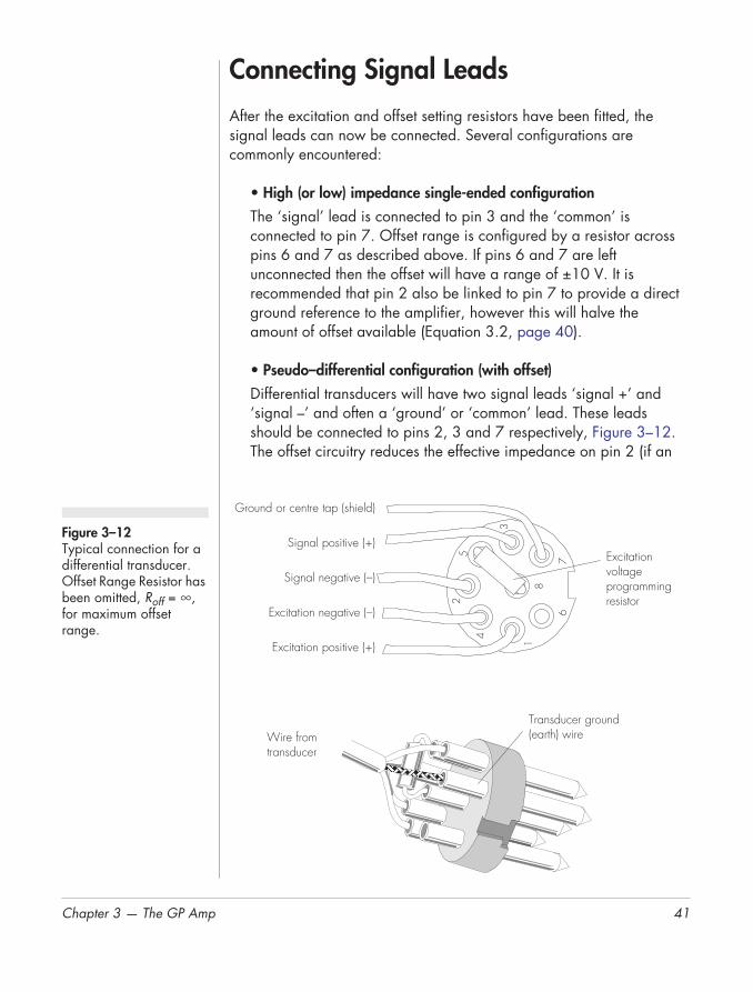
Figure 3–12 Typical connection for a differential transducer. Offset Range Resistor has been omitted, Roff = ∞, for maximum offset range.

Connecting Signal Leads

After the excitation and offset setting resistors have been fitted, the signal leads can now be connected. Several configurations are commonly encountered:

• High (or low) impedance single-ended configuration

The ‘signal’ lead is connected to pin 3 and the ‘common’ is connected to pin 7. Offset range is configured by a resistor across pins 6 and 7 as described above. If pins 6 and 7 are left unconnected then the offset will have a range of ±10 V. It is recommended that pin 2 also be linked to pin 7 to provide a direct ground reference to the amplifier, however this will halve the amount of offset available (Equation 3.2, page 40).

• Pseudo–differential configuration (with offset)

Differential transducers will have two signal leads ‘signal +’ and ‘signal –’ and often a ‘ground’ or ‘common’ lead. These leads should be connected to pins 2, 3 and 7 respectively, Figure 3–12. The offset circuitry reduces the effective impedance on pin 2 (if an

2

3

4

5

67

8



Signal positive (+)

Signal negative (–)


41

1Excitation positive (+)

��

Wire from transducer

Transducer ground (earth) wire

42

Offset Range Resistor is used). This provides a differential (unbalanced) configuration with offset capability, which is suitable for many differential transducers.

• High impedance, true differential configuration

Occasionally, a high impedance, balanced differential configuration is required. In this case the internal link LK3 must to be removed (the GP Amp can be specially ordered in this configuration), and the offset range resistor must not be fitted (consequently there is no offset capability available in this configuration). Differential transducers will have two signal leads ‘signal +’ and ‘signal –’ and often a ‘ground’ or ‘common’ lead. These leads should be connected to pins 2, 3 and 7 respectively.

The transducer cable will normally have a cable shield, which should be connected to pin 7 (ground) of the DIN plug. It is good practice to ensure that the shield is only connected to one ground point, either at the transducer or at the amplifier (but not both) otherwise ground loops will be set up leading to excessive noise. If the casing of the plug is metal, it is good practice to ensure that the casing will also be connected to the shield.

Connecting the Excitation Leads

If balanced positive and negative excitation is required (for example ±5 V). The positive excitation lead is connected to pin 1 and the negative excitation lead is connected to pin 4, Figure 3–12.

If the transducer requires a single supply voltage and a common. The

Bridge & GP Amp

positive supply is connected to pin 1 and the common is connected to pin 7. In these cases the negative excitation is not used and pin 4 is left unconnected.

Testing the Transducer

After connecting the excitation voltage programming resistor, connecting the offset voltage range resistor and wiring up the transducer to the DIN plug, the transducer should now be fully configured for your purposes. The excitation voltage and offset range values will be set automatically when the transducer is plugged into the GP Amp.


Looking at the GP Amplifier dialog box, Figure 3–7 or Figure 3–8, you can see the output from the transducer as you change its operating conditions. You may have to adjust the input range to get a good response. If there appears to be no response from the transducer, recheck the wiring against the diagrams for the appropriate transducer and the manufacturer’s instructions.

43

44
Bridge & GP Amp

Bridge
& GP Amp
A
A P P E N D I X A
Technical Aspects

This appendix describes technical aspects of the Bridge and GP Amplifiers. You do not need to understand the material here to use these amplifiers. It is likely to be of especial interest to the technically minded, providing insights into what these amplifiers can and cannot do, and their suitability for particular purposes. You should not use this material as a service manual: user modification of the Bridge or GP Amp, or the e-corder, voids your rights under warranty.

OverviewThe Bridge Amp, GP Amp, and other eDAQ Amps have been designed to integrate fully with the e-corder system so that the software–controlled gain ranges and filter settings you see in the Chart and Scope software are the combination of both pieces of hardware. The Bridge Amp and GP provide:

45

• additional low drift amplification (chopper stabilized) necessary to deal with the very low signal outputs of most bridge transducers (Bridge Amp only)

• additional programmable filtering, to remove unwanted signal and noise frequencies

• a stable and protected DC excitation voltage supply for powering the transducer where necessary.

• digitally-controlled transducer zeroing or offset circuitry.

The digital control interface used to control filter settings, gain, coupling, and zeroing circuits uses a modified I2C interface system

46

(Phillips), which provides a 4-wire serial communication bus between the e-corder and Amp: all control of the Bridge and GP Amp functions and settings are through this bus. Also present on the I2C connector is a set of regulated power supply rails derived from the e-corder (+17 V, –17 V and +8 V). The eDAQ Amp has its own on–board regulators to generate a stable power supply for the internal circuitry.

The amplified and filtered transducer signal is sent from the eDAQ Amp to the analog input channels of the e-corder via a BNC–to–BNC cable.

The status On–line indicator on an eDAQ Amp is turned on only after the software ‘finds’ or locates the eDAQ amplifier and carries out a two–way dialog with the unit. This requires that the software, drivers, electronics and power supplies are all performing correctly. It does not check the transducer side of the circuit — that is, there will be no warning of a missing or badly connected transducer.

Bridge Amp ConstructionThe overall operation of the Bridge Amps can be better understood by referring to Figure A–1.

The input stage consists of a chopper–stabilized amplifier with (software–controlled) programmable gain of up to ×1000. Secondary amplification is provided by the e-corder to give a total system gain of up to ×200000 (±50 µV full scale). From the input amplifier, the signal is passed to a fifth order, low–pass, switched capacitance filter, the cutoff frequency of which is selected under software control.

Bridge & GP Amp

AC coupling is provided by an integrator feedback loop. This loop forms an effective high–pass filter circuit with a time constant of 1 s. The output of the integrator is fed back into the input terminals of the chopper–stabilised amplifier, thus removing the DC content of the signal. When AC coupling is selected, the automatic zeroing function is disabled.

The excitation voltage is generated by a complementary output stage, derived from a stable internal voltage reference, capable of giving up to ±10 V (20 V DC) excitation at up to 50 mA. The transducer excitation voltage can be adjusted by connecting a resistor between pins 5 and 8 on the connector that plugs into the Bridge Amp’s input

Appendix A — Technical A

Signal input +

Signal input –

Common (ground)

User suppliedoffset range resistor, Roff

Excitation +

Excitation –

On-line indicator

User suppliedexcitation resistor, Rs

Fron

Figure A–1 Block diagram of the Bridge Amp

socket, see Figure 4–1 on page 46. This resistor is usually placed inside the transducer’s DIN connector so that the transducer will be correctly powered when it is attached to the Bridge Amp.

To remove any offsets in a transducer or signal baseline, the Bridge Amp uses a 12 bit DAC (digital–to–analog convertor) to generate an offset voltage. This is internally connected to the input stage when DC coupling is used. Transducer offsets are zeroed by applying a corrective DC voltage to the input stage via the DAC, under software control. In fact current is actually supplied in maximum offset steps of ±0.05 µA, giving a resolution dependent on the transducer impedance.
For example, steps would be about 50 µV for a transducer with
spects 47

impedance of 1 kΩ, less for a transducer with lower impedance.

The DAC is only capable of producing voltages in discrete steps. The offset range can be adjusted downwards by a factor of about ten to decrease the size of these steps and make the zeroing circuit more sensitive, especially at the lower ranges. The range can be adjusted by connecting a resistor between pins 5 and 8 of the transducer connector to Bridge Amp input socket, Figure 2–2 on page 6. The correct offset range for the transducer will always be set when it is attached to the Bridge Amp.

I2C output

I2C input

Analog output

150 kΩ

10 kΩ

150 kΩ

10 kΩ

100 kΩ10 kΩLow pass filters

12 bit DAC

Chopper stabilised amplifier

AC integrator

Back panel

1

2

3

6

7

4

5

8VRef ±10 V

I2 C c

ontro

l in

terfa

cet panel

48

Signal input +

Signal input –

Common (ground)

User suppliedoffset range resistor, Roff

Excitation +

Excitation –

On-line indicator

User suppliedexcitation resistor, Rs

Front

Figure A–2 Block diagram of the GP Amp

GP Amp ConstructionThe block diagram of the GP Amp is shown in Figure A–2.

The input stage consists of a differential amplifier with (software– controlled) programmable gain up to ×1000. Secondary amplification is provided by the e-corder to give a total system gain of up to ×5000 (±2 mV full scale). From the input amplifier, the signal is passed to a selection of three 4–pole linear filters. The filter allows a range of cutoff frequencies to be selected under software control. A ‘Filter off’ position
allows the full bandwidth of the amplifier to be employed.
Bridge & GP Amp

The excitation voltage is generated by a complementary output stage, derived from a stable internal voltage reference, capable of giving up to ±10 V (20 V DC) excitation at up to 50 mA. The transducer excitation voltage can be adjusted by connecting a resistor between pins 5 and 8 on the connector that plugs into the GP Amp’s input socket, see Figure 3–2 on page 26. This resistor is usually placed inside the transducer’s DIN connector so that the transducer will be correctly powered when it is attached to the GP Amp.

To remove any offsets in a transducer or signal baseline, the GP Amp uses a 12 bit DAC (digital–to–analog convertor) to generate an offset

Differential Amplifier

LK3

12 bit DAC

VRef ±10 V I2 C c

ontro

l in

terfa

ce

1

2

3

6

7

4

5

8

I2C output

I2C input

Analog output

Low pass filters

Back panel panel

150 kΩ

150 kΩ

10 kΩ

100 kΩ

10 kΩ

10 kΩ

Appendix A — Technical A

voltage. Signal offsets are zeroed by applying a corrective DC voltage to the negative input stage, under software control. The input amplifier under these circumstances functions as a high impedance single–ended amplifier.

The DAC is only capable of producing voltages in discrete steps. The offset range (and the size of the steps) can be decreased by a factor of about ten to make the zeroing circuit more sensitive. The range can be adjusted by connecting a resistor between pins 6 and 7 of the transducer plug, Figure 3–11 on page 39. The correct offset range for the transducer will then always be set when it is attached to the GP Amp.

If you wish to use the GP Amp to provide a high impedance fully differential input then the internal link marked LK3 must be removed, and the offset range resistor, Rs, between pins 6 and 7 must not be fitted to the transducer plug. This also renders the DC offset inoperative.

AC coupling (high pass filtering with a time constant of about 0.3 s) can be selected in software. This is provided by an RC network at the input. This setting is useful if small fast signal oscillations need to be observed superimposed on a larger DC background. DC offset is not provided in this mode.

spects 49

50
Bridge & GP Amp

Bridge
& GP Amp
B
A P P E N D I X B
Troubleshooting

This appendix describes some of the more common problems that can occur, how they are caused, and what you can do to fix them. If you continue to have difficulties then please your eDAQ representative or e–mail [email protected].

Most of the problems that you are likely to encounter are caused by loose or missing connections. In the even of a problem always check all connections and re–start the hardware and software. It is also imperative that the transducer plug be wired correctly as outlined in Chapters 3 and 4. Only rarely will there be an actual problem with the Bridge or GP Amp or the e-corder itself.

The eDAQ Amp is not recognised by the Chart or Scope software.

• In this case the Status indicator on front panel of the Bridge or GP Amp will fail to light when the software is started. Also the software will indicate ‘Input Amplifier…’ rather than ‘Bridge Amp…’

51

or ‘GP Amp…’ on the channel to which the eDAQ Amp is connected. The Status indicator is turned on at the end of a bidirectional dialog between the e-corder unit and the eDAQ Amp after the software checks most of the functions of the eDAQ Amp. This dialog will fail if the I2C cable or the BNC–to–BNC cables from the eDAQ Amp to the e-corder are not be connected, or are loose. Check to see that all cables are firmly attached. The BNC cables must be connected to an e-corder input channel (not the e-corder output!). Make sure you are looking at the software channel that corresponds to the input channel to which the eDAQ Amp is connected. You will need to re–start the software after changing or adjusting cables.

52

• The BNC or I2C cable may be faulty. Replace the cable (if possible) and try again. Spare cables are available from many electronics suppliers or can be obtained from your eDAQ representative. You will need to re–start the software after changing or adjusting cables.

• The eDAQ Amp or e-corder may have developed a fault. This is the less likely than problems discussed above. Try using the eDAQ amp on another e-corder (if available), or try using a different eDAQ Amp (if available) on the e-corder. If you feel that you have a faulty unit please contact your eDAQ representative.

On starting up the software, an alert indicates that there is a problem with the eDAQ Amp or driver. This will also prevent the Status Indicator from being turned ON.

• The correct eDAQ Amp driver is not installed or is missing on your computer. Reinstall the Chart and Scope software.

• The BNC or I2C cable is faulty, or there may be a faults with the eDAQ Amp or the e-corder (proceed as in the previous section).

The trace will not zero properly when using the automatic or manual zeroing controls.

• Variations in the transducer signal during auto–zeroing procedure can cause the software to fail to zero properly. Make sure that the transducer is providing a steady signal during auto–zeroing.

• If the transducer is defective or subject to excessive load, it could cause the offset range of the eDAQ Amp’s zeroing circuitry to be exceeded.

Bridge & GP Amp

• Check the transducer with another Bridge (or GP) Amp if possible and try again. If you have bought the transducer from a supplier other than eDAQ then you will have wired the transducer connector yourself. Please check your wiring and values of the excitation and offset resistors. Excessive excitation could be causing heating of the transducer and a drifting signal. An incorrectly selected offset resistor will provide insufficient (or too much) offset.

Appendix B — Troubleshoo

The signal from the transducer is noisy at high gain ranges

• No transducer is completely noise free, and with sufficient amplification noise will become apparent. Noise can be reduced by the use of low pass filtering.

• If you suspect mains hum or signal interference from other sources (your PC and monitor can be a noise source) record the noise data at high speed for a few seconds with the Chart software. Then perform a Spectrum on the recorded data. The frequencies of mains hum (50 or 60 Hz and harmonics thereof) and other noise sources will be visible as peaks in the power spectrum. This information is sometimes useful in identifying the source of the noise.

There is no, or only a small, signal from the transducer, even at high gain ranges

• Check that you have selected a sufficiently sensitive gain range on the Bridge or GP Amp.

• Try to identify if the problem lies with the transducer or with the Bridge (or GP) Amp by checking how the transducer performs with another Bridge (or GP) Amp if possible. Also try a similar transducer with the Bridge (or GP) Amp if possible. If the problem located within the transducer, then check the transducer plug wiring as below. If you feel the problem resides in the Bridge (or GP) Amp then please contact your eDAQ representative.

• The wiring in the transducer plug could be loose or incorrect. If you have wired your own transducer plug, check the wiring and soldering within the plug.

ting 53

• Excitation (power) to the transducer could be insufficient or missing. Check the wiring in the transducer plug and confirm that an excitation resistor of the correct size has been fitted.

54
Bridge & GP Amp

Bridge
& GP Amp
C
A P P E N D I X C
Specifications

Bridge AmpInput

Connector: 8–pin DIN socket

Input configuration: Differential or single–ended

Amplification range: ±50 µV to ±200 mV full scale in 12 steps (combined e-corder and Bridge Amp)±200, 100, 50, 20, 10, 5, 2, 1mV±500, 200, 100, 50 µV

Amplification accuracy: ±0.5% (combined e-corder and Bridge Amp)

Maximum input voltage: ±5 V

55

Input impedance: 2 × 10 kΩ

Low-pass filtering: 1 Hz to 2 kHz in eight steps (software selectable), using fifth order, switched capacitance filter type

High-pass filtering: DC (off) or 0.1 Hz (software–selectable)

Frequency response (–3 dB): 2 kHz maximum at all gains with the 2 kHz filter selected

CMRR (differential): 100 dB @ 50 Hz (typical)

Input noise: <2 µVrms referred to input at highest gain

56

Excitation and Zeroing

DIN Excitation voltage range:0 – 20 V DC (±10 V referred to ground), adjusted by external resistor

Transducer drive current: ±50 mA maximum

Zeroing circuitry: Software-controlled, either manual or automatic

Internal offset resolution: 12–bit (internal DAC) 0 V ± 2048 steps. Maximum offset steps of 5 µA, giving a resolution of about 0.15 mV for a transducer impedance of 300 Ω.

Control Port

I2C input and output: Male and female DB–9 pin connectors. Provides control and power.

Power requirements: ±17 V DC+8 V DC3.2 W (without transducer)

Physical ConfigurationDimensions (h × w × d): 50 × 76 × 260 mm

1.96 × 3.0 × 10.2 inches

Weight: 0.8 kg (1.8 lb)

Operating conditions: 0 – 35˚C0 – 90% humidity (non–condensing)

Bridge & GP Amp

eDAQ reserves the right to alter these specifications at any time.

Appendix C — Specificatio

GP AmpInput

Connector: 8–pin DIN socket

Input configuration: Differential or single–ended

Amplification ranges: ±2 mV to ±10 V full scale in 12 steps (combined e-corder and GP Amp)±10, 5, 2, 1V±500, 200, 100, 50, 20, 10, 5, 2 mV

Amplification accuracy: ±0.5% (combined e-corder and GP Amp)

Maximum input voltage: ±15 V

Input impedance: 100 MΩ

Frequency response (–3 dB): 5 kHz maximum at all gains with filters off

CMRR (differential): 100 dB @ 50 Hz (typical)

Input noise: <2 µVrms referred to input at highest gain

Excitation and Zeroing

Excitation voltage range: 0 – 20 V DC (±10 V referred to ground), adjusted by external resistor

Transducer drive current: ±50 mA maximum

Zeroing circuitry: Software–controlled, either manual or automatic

ns 57

Internal offset resolution: 12–bit (internal DAC) 0 V ± 2048 steps. Designed to offset a maximum of ±5 V, giving a resolution of about 2.5 mV.

Filters

Bandwidth: 5 kHz (Low pass filters set to Off)

Low pass filtering: Fourth order Bessel1, 10, or 100 Hz (software–selectable)

High pass filtering: DC (off) or 0.3 Hz (software–selectable)

58

Control Port

I2C input and output: Male and female DB–9 pin connectors. Provides control and power.

Power requirements: ±17 V DC+8 V DC3.2 W (without transducer)

Physical ConfigurationDimensions (h × w × d): 50 × 76 × 260 mm

1.96 × 3.0 × 10.2 inches

Weight: 0.8 kg (1.8 lb)

Operating conditions: 0 – 35˚C0 – 90% humidity (non–condensing)

eDAQ reserves the right to alter these specifications at any time.

Bridge & GP Amp

Appendix C — Specificatio
ns 59

60
Bridge & GP Amp

Bridge

conne

DDAC 1differe

odigitadispla

BG

Index

AAC coupling


automatic zeroingBridge Amp 13GP Amp 33

Bback panel


block diagramBridge Amp 47GP Amp 48

Bridge Amp 2

Cchecking the eDAQ Amp 3

EeDAQ Amps 2

Bridge Amp 2GP Amp 2pH/mV Amp 2Picostat 2Potentiostat 2

eDAQ web site 2excitation voltage


Ffiltering


front panelBridge Amp 6GP Amp 26

full–bridge transducers 21

GP Amp

& GP Amp 61

cting multiple eDAQ Amps 8, 28

9, 39ntial transducerffset required 41l-to-analog converter 19, 39, 47, 48y offsetridge Amp 13P Amp 33

GGP Amp 2

Hhalf–bridge transducers 21high impedance transducers

differential 42single–ended 41

high–pass filterBridge Amp 46GP Amp 49

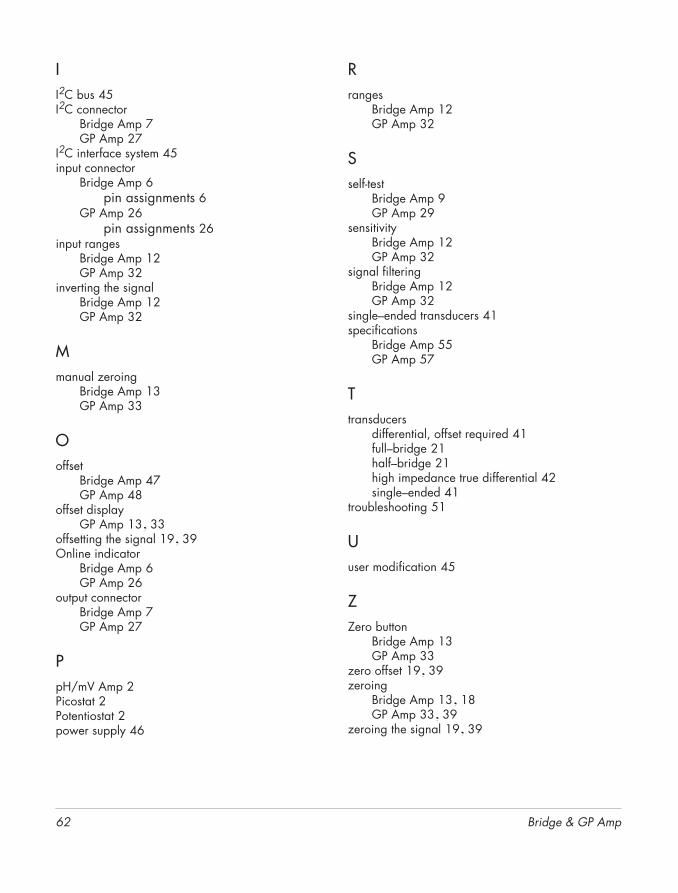
II2C bus 45I2C connector


I2C interface system 45input connector

Bridge Amp 6pin assignments 6

GP Amp 26pin assignments 26

input rangesBridge Amp 12GP Amp 32

inverting the signalBridge Amp 12GP Amp 32

Mmanual zeroing


Ooffset


offset displayGP Amp 13, 33

offsetting the signal 19, 39Online indicator

Bridge Amp 6

Rranges


Sself-test


sensitivityBridge Amp 12GP Amp 32

signal filteringBridge Amp 12GP Amp 32

single–ended transducers 41specifications


Ttransducers

differential, offset required 41full–bridge 21half–bridge 21high impedance true differential 42single–ended 41

troubleshooting 51

Uuser modification 45

62 Bridge & GP Amp

GP Amp 26output connector


PpH/mV Amp 2Picostat 2Potentiostat 2power supply 46

ZZero button


zero offset 19, 39zeroing

Bridge Amp 13, 18GP Amp 33, 39

zeroing the signal 19, 39

Bridge

problethis Ag

Hard

eDAQfree oyear frepairappro

To obfirst nowill iss

LicensinBridge Amp

Trademarks

e-corder and PowerChrom are registered trademarks of eDAQ Pty Ltd. All eDAQ software, hardware, and documentation is protected by copyright. eDAQ retains the exclusive ownership of the trademarks and registered trademarks represented by its company name, logo, and product names.

Responsibilities

You and any others using any eDAQ product agree to use it in a sensible manner for purposes for which it is suited, and agree to take responsibility for their actions and the results of their actions.

If problems arise with an eDAQ product, eDAQ will make all reasonable efforts to fix them. This service may incur a charge, depending on the nature of the

& GP Amp

ms, and is subject to the other conditions in reement.

ware Warranty

Pty Ltd warrants the Bridge or GP Amp, to be f defects in material and workmanship for one rom the date of purchase. eDAQ Pty Ltd will or replace defective equipment as priate.

tain a warranty repair/replacement you must tify us before return of the instrument and we ue you with a RAN (return authorization

g & Warranty

number). You must ship the defective product at your expense. We will pay return shipping. The product should be packed safely (preferably in its original packaging) and have the RAN on the shipping label. Returns sent without a RAN may be refused delivery.

This warranty does not cover hardware that has:

• been modified by the user in any way;

• been subjected to unusual physical, electrical, or environmental stress. This includes damage due to faulty power sockets, inadequate earthing, or power spikes or surges;

• been damaged because of incorrect wiring to ancillary equipment, or because of substandard, connectors or cables; or

• had the original identification marks removed or altered.

63

Software License

You have the non-exclusive right to use the supplied eDAQ software (Chart, Scope etc). Your employees or students, for example, are entitled to use it, provided they adhere to this agreement. Each separate purchase of the eDAQ software licenses it to be used on two computers at any given time (on one computer for data acquisition with a e-corder hardware unit, and on a second computer for the analysis of existing data files). Although multiple copies of a program may exist on several computers, more than two copies must not be used

simultaneously. Departmental/company licences are available if you wish to run more than two copies simultaneously.

Technical Support

Please register your unit to receive technical support. Technical assistance is available via email. Please describe the problem with as much detail as possible. Include a small example data file, if appropriate. Please also state:

• the model and serial number of your e-corder unit and Bridge or GP Amp.

• the type of computer and operating system being used (for example Windows XP, or Macintosh OS 10.2)

• the software version you are using (for example Chart v5.1.2)

We endeavor to answer all your questions, but in some cases, for example where the problem relates to the other equipment that you are using, a nominal fee may be charged.

Jurisdiction

64

eDAQ Pty Ltd is bound by the laws of New South Wales in Australia, and any proceedings shall be heard by the Supreme Court of New South Wales in Australia.

Disclaimer

eDAQ reserves the right to alter specifications of hardware and software without notice.

No liability can be accepted for consequential damages resulting from use of eDAQ products.

Bridge & GP Amp

bridge & gp amp book

Documents