Prepared for submission to JHEP

Bremsstrahlung function, leading Luscher correction

at weak coupling and localization

Marisa Boninia, Luca Griguoloa, Michelangelo Pretia and Domenico Seminarab

a Dipartimento di Fisica e Scienze della Terra, Universita di Parma and INFN Gruppo Collegato

di Parma, Viale G.P. Usberti 7/A, 43100 Parma, Italyb Dipartimento di Fisica, Universita di Firenze and INFN Sezione di Firenze, via G. Sansone 1,

50019 Sesto Fiorentino, Italy

E-mail: marisa.bonini@fis.unipr.it, luca.griguolo@fis.unipr.it,

michelangelo.preti@fis.unipr.it, domenico.seminara@fi.infn.it

Abstract: We discuss the near BPS expansion of the generalized cusp anomalous dimen-

sion with L units of R-charge. Integrability provides an exact solution, obtained by solving

a general TBA equation in the appropriate limit: we propose here an alternative method

based on supersymmetric localization. The basic idea is to relate the computation to the

vacuum expectation value of certain 1/8 BPS Wilson loops with local operator insertions

along the contour. These observables localize on a two-dimensional gauge theory on S2,

opening the possibility of exact calculations. As a test of our proposal, we reproduce the

leading Luscher correction at weak coupling to the generalized cusp anomalous dimension.

This result is also checked against a genuine Feynman diagram approach in N = 4 Super

Yang-Mills theory.

Keywords: Wilson, ’t Hooft and Polyakov loops, Duality in Gauge Field Theories, 1/N

Expansion

arX

iv:1

511.

0501

6v2

[he

p-th

] 2

7 N

ov 2

015

Contents

1 Introduction 1

2 Loop operators in N = 4 SYM and YM2: an alternative route to the

generalized Bremsstrahlung function 4

2.1 BPS wedge on S2 with scalar insertions in N = 4 SYM 6

2.2 The wedge on S2 with field strength insertions in YM2 7

3 Perturbative computation of the Luscher term from YM2 on the sphere 8

3.1 General setting for perturbative computations on S2 9

3.2 Operator insertions of length L = 1 9

3.3 Operator insertions of length L 13

4 The L = 1 case from perturbative N = 4 SYM 16

5 Conclusions and outlook 19

Appendix 20

A The generating function G(t, ε, z) and some related properties 20

1 Introduction

In the last few years we have observed surprising applications of powerful quantum field

theoretical techniques to N = 4 Super Yang-Mills (SYM) theory. In particular the in-

vestigation of integrable structures [1] and the use of supersymmetric localization [2] have

produced a huge number of results that are beyond perturbation theory and can be suc-

cessfully compared with AdS/CFT expectations. For example the exact spectrum of single

trace operator scaling dimensions can be obtained through TBA/Y-system equations [3–6]

or, more efficiently, using the approach of the Quantum Spectral Curve (QSC) [7]. Su-

persymmetric Wilson loops and classes of correlation functions can be instead computed

– 1 –

exactly via supersymmetric localization, that exploit the BPS nature of the related ob-

servables [8–15]. It is certainly interesting to understand the relation between these two

approaches, when the same quantities can be computed in both ways.

An important object, appearing in gauge theories is the cusp anomalous dimension Γ(ϕ),

that was originally introduced in [16, 17] as the ultraviolet divergence of a Wilson loop

with Euclidean cusp angle ϕ. In supersymmetric theories Γ(ϕ) is not BPS, due to the pres-

ence of the cusp, and defines in the light-like limit ϕ→ i∞ an universal observable: exact

results have been derived in N = 4 SYM through integrability [18] that match both weak

coupling expansions [19] and string computations describing the strong coupling behavior

[20]. A related TBA approach, that goes beyond the light-like limit, was later proposed

[21, 22]: the cusp anomalous dimension can be generalized including an R-symmetry angle

θ that controls the coupling of the scalars to the two halves of the cusp [23]. The system

interpolates between BPS configurations (describing supersymmetric Wilson loops) and

generalized quark-antiquark potential: exact equations can be written applying integrabil-

ity, and have been checked successfully at three loops [21]. For a recent approach using the

QSC see [24]. Moreover one can use localization in a suitable limit to obtain the exact form

of the infamous Bremsstrahlung function [25], that controls the near-BPS behavior of the

cusp anomalous dimension (see also [26] for a different derivation). The same result has

been later directly recovered from the TBA equations [27, 28] and QSC method [24, 29].

It is clear that the generalized cusp anomalous dimension Γ(θ, ϕ) represents, in N = 4

SYM, a favorable playground in which the relative domains of techniques as integrability

and localization overlap.

The fundamental step that allowed to derive exact equations for Γ(θ, ϕ) from integrability

was to consider the cusped Wilson loop with the insertion of L scalars Z = Φ1 + iΦ2 on

the tip. Importantly the scalars appearing in Z should be orthogonal to the combinations

that couple to the Wilson lines forming the cusp. The anomalous dimension ΓL(θ, ϕ) of the

corresponding Wilson loop depends on L-unit of R-charge and a set of exact TBA equations

can be written by for any value of L, θ and ϕ: setting L = 0 one of course recovers Γ(θ, ϕ).

When ϕ = ±θ the operator becomes BPS and its near-BPS expansion in (ϕ − θ) can be

studied directly from the integrability equations. The leading coefficient in this expansion

is called the Bremsstrahlung function when L = 0 and its expression has been derived to

all loops from localization [25]. For θ = 0 it was reproduced at any coupling in [27] by the

analytic solution of the TBA, which also produced a new prediction for arbitrary L. The

extension to the case with arbitrary (θ− ϕ) and any L is presented in [28]. The near-BPS

results for L ≥ 1 can be rewritten as a matrix model partition function whose classical

limit was investigated in [29] giving the corresponding classical spectral curve. A related

approach based on a QSC has been proposed in [24], reproducing the above results.

In this paper we generalize the localization techniques of [25] to the case of ΓL(θ, ϕ),

checking the prediction from integrability. Having an alternative derivation of the results

may shed some light on the relations between these two very different methods. We consider

here the same 1/4 wedge BPS Wilson loop used in [25], with contour lying on an S2 subspace

– 2 –

of R4 or S4, inserting at the north and south poles, where the BPS cusp ends, L ”untraced”

chiral primaries of the type introduced in [15, 30]. The analysis of the supersymmetries

presented in [13] shows1 that the system is BPS. Following exactly the same strategy of

[25] we can relate the near BPS limit of ΓL(θ, ϕ) to a derivative of the wedge Wilson

loop with local insertions and define a generalized Bremsstrahlung function BL(λ, ϕ) as

in [27]. Our central observation is that the combined system of our Wilson loop and

the appropriate local operator insertions still preserves the relevant supercharges to apply

the localization procedure of [13] and the computation of BL(λ, ϕ) should be therefore

possible in this framework. As usual supersymmetric localization reduces the computation

of BPS observables on a lower dimensional theory (sometimes a zero-dimensional theory

i.e a matrix model) where the fixed points of the relevant BRST action live. For general

correlation functions of certain 1/8 BPS Wilson loops and local operators inserted on

a S2 in space-time, localization reduces N = 4 SYM to a 2d Hitchin/Higgs-Yang-Mills

theory, that turns out to be equivalent to the two-dimensional pure Yang-Mills theory

(YM2) on S2 in its zero-instanton sector2. In particular the four-dimensional correlation

functions are captured by a perturbative calculation in YM2 on S2. In two dimensions,

the preferred gauge choice is the light-cone gauge, since then there are no interactions:

the actual computations are drastically simplified thanks to the quadratic nature of the

effective two-dimensional theory. This sort of dimensional reduction has passed many non-

trivial checks [31–36], comparing the YM2 results both at weak coupling (via perturbation

theory in N = 4 SYM) and strong coupling (using AdS/CFT correspondence).

Here we investigate the near-BPS limit of ΓL(θ, ϕ) using perturbative YM2 on the sphere:

more precisely we attempt the computation of BL(λ, ϕ). The problem of resumming in this

case the perturbative series in YM2 is still formidable (we will come back on this point in

the conclusions) and we limit ourselves here to the first non-trivial perturbative order. In so

doing we recover, in closed form, the leading Luscher correction to the ground state energy

of the open spin chain, describing the system in the integrability approach (λ = g2N)

ΓL(θ, ϕ) ' (ϕ− θ) (−1)LλL+1

4π(2L+ 1)!B2L+1

(π − ϕ

2π

), (1.1)

where Bn(x) are the Bernoulli polynomials. This correction was computed in [21, 22], fol-

lowing directly from the TBA equations, and checked from the general formulae in [27, 28].

Interestingly it was also reproduced in [37] by a direct perturbative calculation in some ap-

parently unrelated amplitude context. We think that our result not only represents a strong

check that our system computes the generalized Bremsstrahlung function but also suggests

some relations between two-dimensional diagrams and four-dimensional amplitudes.

The plan of the paper is the following: in Section 2 we present the construction of the wedge

Wilson loop in N = 4 SYM with the relevant operator insertions. We discuss the BPS

1Actually in [15] it was proved that a general family of supersymmetric Wilson loops on S2 and the local

operators OL(x) = tr(Φn + iΦB)L share two preserved supercharges.2Truly to say, to complete the proof of [13] one should still evaluate the one-loop determinant for the

field fluctuations in the directions normal to the localization locus. However, there are many reasons to

believe that such determinant is trivial.

– 3 –

nature of these observables and their mapping to two-dimensional Yang-Mills theory on S2

in the zero-instanton sector. The relation with the generalized Bremsstrahlung function is

also established. In Section 3 we set up the perturbative calculation of the first non-trivial

contribution to the near-BPS limit of ΓL(θ, ϕ), first considering the case L = 1 and then

presenting the computation for general L. We recover the weak coupling contribution to

the Luscher term as expected. In Section 4 we perform the L = 1 computation using

Feynman diagrams in N = 4 SYM: this is a check of our construction and also exemplifies

the extreme complexity of the conventional perturbative calculations. In Section 5 we

present our conclusions and perspectives, in particular discussing how the full result for

BL(λ, ϕ) could be recovered and its matrix model formulation should arise from YM2 on

the sphere. Appendix A is instead devoted to some technical aspects of YM2 computation.

2 Loop operators in N = 4 SYM and YM2: an alternative route to the

generalized Bremsstrahlung function

For the N = 4 SYM theory an interesting and infinite family of loop operators which

share, independently of the contour, 18 of the original supersymmetries of the theory were

constructed in [11, 12]. They compute the holonomy of a generalized connection combining

the gauge field (Aµ), the scalars (ΦI) and the invariant forms (εµνρdxνxρ) on S2 as follows

(we follow the conventions of [14])

W =1

NTr

[Pexp

(∮dτ (xµAµ + iεµνρx

µxνΦρ)

)]. (2.1)

Above we have parameterized the sphere in terms of three spatial cartesian coordinates

obeying the constraint x21 + x2

2 + x23 = 1. The normalization N is the rank of the unitary

gauge group U(N).

In [11, 12] it was also argued that the expectation value of this class of observables was

captured by the matrix model governing the zero-instanton sector of two dimensional Yang-

Mills on the sphere:

〈W(2d)〉 =1

Z

∫DM

1

NTr(eiM

)exp

(− A

g22dA1A2

Tr(M2)

)=

=1

NL1N−1

(g2

2dA1A2

2A

)exp

(−g2

2dA1A2

4A

),

(2.2)

where A1, A2 are the areas singled out by the Wilson loop and A = A1 + A2 = 4π is the

total area of the sphere. The result in N = 4 SYM is then obtained with the following

map

g22d 7→ −

2g2

A. (2.3)

Above g2d and g are respectively the two and four dimensional Yang-Mills coupling con-

stants.

– 4 –

This intriguing connection between YM2 and N = 4 SYM was put on solid ground by

Pestun in [2, 13]. By means of localization techniques, he was able to argue that the four-

dimensional N = 4 Super Yang-Mills theory on S4 for this class of observables reduces

to the two-dimensional constrained Hitchin/Higgs-Yang-Mills (cHYM) theory on S2. The

Wilson loops in the cHYM theory are then shown to be given by those of YM2 in the zero

instanton sector. These results were extended to the case of correlators of Wilson loops

in [15, 32] and to the case of correlators of Wilson loop with chiral primary operators in

[14, 15].

The knowledge of the exact expectation value for this family of Wilson loops has been

a powerful tool to test the AdS/CFT correspondence in different regimes. In particular,

here, we want to investigate the connection, originally discussed in [25], between these

observables and the so-called Bremsstrahlung function.

Consider, in fact, the generalized cusp Γ(θ, ϕ) defined in [23], namely the coefficient of

the logarithmic divergence for a Wilson line that makes a turn by an angle ϕ in actual

space-time and by an angle θ in the R−symmetry space of the theory. When θ = ±ϕthe Wilson line becomes supersymmetric and Γ(θ, ϕ) identically vanishes. In this limit the

operator is, in fact, a particular case of the 14 BPS loops discussed by Zarembo in [38]. In

[25] a simple and compact expression for the first order deviation away from the BPS value

was derived. When |θ − ϕ| � 1, we can write

Γ(θ, ϕ) ' −(ϕ− θ)H(λ, ϕ) +O((ϕ− θ)2) (2.4)

where

H(λ, ϕ) =2ϕ

1− ϕ2

π2

B(λ) with λ = λ

(1− ϕ2

π2

). (2.5)

In (2.5) B(λ) is given by the Bremsstrahlung function of N = 4 SYM theory.

The expansion (2.4) was obtained in [25] by considering a small deformation of the so-called14 BPS wedge. It is a loop in the class (2.1) which consists of two meridians separated by

an angle π − ϕ. The analysis in [25] in particular shows that H(λ, ϕ) can be computed as

the logarithmic derivative of the expectation value of the BPS wedge with respect to the

angle ϕ

H(λ, ϕ) = −1

2∂ϕ log 〈Wwedge(ϕ)〉 = −1

2

∂ϕ〈Wwedge(ϕ)〉〈Wwedge(ϕ)〉

. (2.6)

The quantity 〈Wwedge(ϕ)〉 is given by the matrix model (2.2) with the replacement (2.3).

In other words 〈Wwedge(ϕ)〉 = 〈Wcircle(λ)〉 where λ is defined in (2.5).

The results (2.5) and (2.6) were also recovered in [27, 28] by solving the TBA equations,

obtained in [21], for the cusp anomalous dimension in the BPS limit. This second ap-

proach based on integrability naturally led to consider a generalization ΓL(θ, ϕ) for the

cusp anomalous dimension, where one has inserted the scalar operator ZL on the tip of

the cusp3. In [28] it was shown that the whole family ΓL(θ, ϕ) admits an expansion of the

3 The scalar Z is the holomorphic combination of two scalars, which do not couple to the Wilson line.

– 5 –

type (2.4) when |θ − ϕ| � 1 :

ΓL(θ, ϕ) ' −(ϕ− θ)HL(λ, ϕ) +O((ϕ− θ)2) (2.7)

with

HL(λ, ϕ) =2ϕ

1− ϕ2

π2

BL(λ, ϕ) . (2.8)

The function BL(λ, ϕ) is a generalization of the usual Bremsstrahlung function and its

value for any L in the large N limit was derived in [28].

Below, we want to show that expansion (2.7) and in particular the function BL(λ, ϕ) can

be evaluated exploiting the relation between the Wilson loops (2.1) and YM2 as done in

[25] for the case L = 0.

2.1 BPS wedge on S2 with scalar insertions in N = 4 SYM

The first step is to construct a generalization of the 14 BPS wedge in N = 4 SYM, whose

vacuum expectation value is still determined by a suitable observable in YM2. We start by

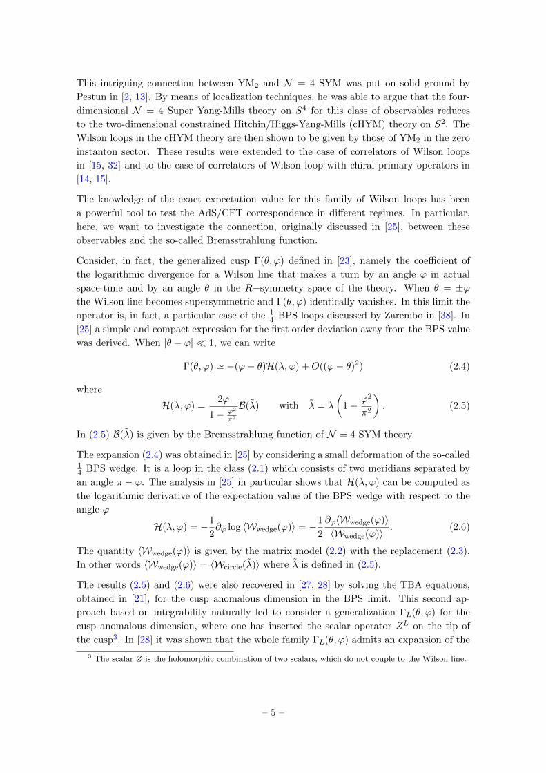
Figure 1: Pictorial description of the observable (2.13): the 14 BPS wedge with operator insertions

in the north and the south pole.

considering the contour depicted in Figure 1, namely the wedge composed by two meridians

Cl and Cr, the first in the (x1, x3) plane and the second in a plane with longitude angle δ:

Cl 7→ xµl = (sin τ, 0, cos τ) 0 ≤ τ ≤ π,Cr 7→ xµr = (− cos δ sinσ,− sin δ sinσ, cosσ) π ≤ σ ≤ 2π.

(2.9)

On the two meridians the Wilson loop couples to two different combinations of scalars.

Indeed the effective gauge connections on the two sides are given by

Al = xµl Aµ − iΦ2 , Ar = xµrAµ − i sin δΦ1 + i cos δΦ2. (2.10)

We now consider the insertion of local operators in the loop and focus our attention on

those introduced in [30] and studied in detail in [14]. They are given by:

OL(x) =(xµΦµ + iΦ4

)L, (2.11)

– 6 –

where xµ are the cartesian coordinate of a point on S2 and the index µ runs from 1 to 3.

Any system of these operators preserves at least four supercharges. When the Wilson loops

(2.1) are also present, the combined system is generically invariant under two supercharges(116 BPS

)[15]. Here we choose to insert two of these operators: one in the north pole

[xµN = (0, 0, 1)] and the other in the south pole [xµS = (0, 0,−1)]. In these special positions

they reduce to the holomorphic and the anti-holomorphic combination of two of the scalar

fields which do not couple to the loop

OL(xN ) =(Φ3 + iΦ4

)L ≡ ZL , OL(xS) =(−Φ3 + iΦ4

)L ≡ (−1)LZL. (2.12)

Then the generalization of the 14 BPS wedge which is supposed to capture the generalized

Bremsstrahlung function BL(λ, ϕ) is simply given by

WL(δ) = Tr

[ZL Pexp

(∫Cl

Aldτ)ZL Pexp

(∫Cr

Ardσ)]

. (2.13)

The operators (2.13) preserve 18 of the supercharges. Applying the same argument given

in [25], one can argue (since the relevant deformation never involves the poles) that

HL(λ, ϕ) =2ϕ

1− ϕ2

π2

BL(λ, ϕ) =1

2∂δ log 〈WL(δ)〉

∣∣∣∣δ=π−ϕ

. (2.14)

2.2 The wedge on S2 with field strength insertions in YM2

Next we shall construct a putative observable in YM2, which computes the vacuum ex-

pectation of WL(δ). Following [12], we map the Wilson loop of N = 4 SYM into a loop

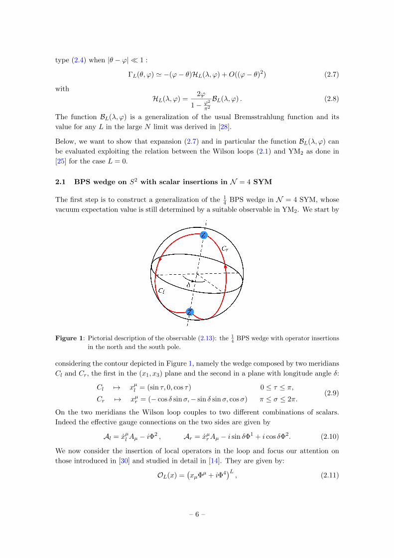
Figure 2: Wedge on S2 in stereographic coordinates. The blue blobs denote the operator insertions.

operator of YM2 defined along the same contour C on S2. Since we use the complex stere-

ographic coordinates z = x + iy to parametrize the sphere, the wedge will appear as an

infinite cusp on the plane where the origin represents the north pole, while the infinity is

identified with the south pole (see Figure 2). The two straight-lines C1 and C2 are then

given by

C1 7→ z(t) = t t ∈ [∞, 0] ,

C2 7→ w(s) = eiδs s ∈ [0,∞] .(2.15)

– 7 –

In these coordinates the metric on S2 takes the usual conformally flat form

ds2 =4dzdz

(1 + zz)2. (2.16)

The wedge Wilson loop is mapped into

WC =1

NTr

[Pexp

(∮Cdτ zAz(z)

)], (2.17)

where C = C1 ∪ C2 (see Figure 2). In (2.17) we have used the notation A, to distinguish

gauge field in d = 2 from its counterpart A in d = 4.

The two dimensional companion of the operator (2.11) was found in [14] through a local-

ization argument. These local operators are mapped into powers of the field strength F of

the two-dimensional gauge field A:

OL(x) 7→(i ∗F (z)

)L. (2.18)

Here the ∗ denotes the usual hodge dual on the sphere. Combining the above ingredients

the observable in YM2 which computes the vacuum expectation value of (2.13) is

W(2d)L (δ) = Tr

[(i ∗F (0)

)LPexp

(∫C2

wAwds

) (i ∗F (∞)

)LPexp

(∫C1

zAzdt

)].

(2.19)

Constructing a matrix model for the observable (2.19) in the zero instanton sector is neither

easy nor immediate. In fact the usual topological Feynman rules for computing quantities

in YM2 are tailored for the case of correlators of Wilson loops. The insertion of local

operators along the contour was not considered previously and the rules for this case are

still missing. Therefore, in the next section, to test the relation between the function

HL(λ, ϕ) and the vacuum expectation value of (2.19) implied by (2.14), i.e.

HL(λ, ϕ) =2ϕ

1− ϕ2

π2

BL(λ, ϕ) =1

2∂δ log 〈W(2d)

L (δ)〉∣∣∣∣ δ=π−ϕg22d

=−2g2/A

, (2.20)

we shall resort to standard perturbative techniques.

3 Perturbative computation of the Luscher term from YM2 on the sphere

In this Section we compute the first non-trivial perturbative contribution to the generalized

Bremsstrahlung function BL(λ, ϕ), in the planar limit, using perturbation theory in YM2. It

coincides with the weak coupling limit of the Luscher term, describing wrapping corrections

in the integrability framework. We believe it is instructive to present first the computation

for L = 1, where few diagrams enter into the calculation and every step can be followed

explicitly. Then we turn to general L, exploiting some more sophisticated techniques to

account for the combinatorics.

– 8 –

3.1 General setting for perturbative computations on S2

For perturbative calculations on the two dimensional sphere, it is convenient to use the

holomorphic gauge Az = 0. In this gauge the interactions vanish and the relevant propa-

gators are:

〈(Az)ij(z)(Az)kl (w)〉 = −g2

2d

2πδilδ

kj

1

1 + zz

1

1 + ww

z − wz − w

,

〈(i∗F ij (z))(i∗F kl (w))〉 = −δilδkj(g2

2d

8π−ig2

2d

4(1 + zz)2δ(2)(z − w)

),

〈(i∗F ij (z))(Az)kl (w)〉 = −g2

2d

4πδilδ

kj

1

1 + ww

1 + zw

z − w.

(3.1)

When computing the above propagators for points lying on the edge C1 (z = t) and on the

edge C2 (w = eiδs), they reduce to

〈(Az)ij(z)(Az)kl (w)〉 = −g2

2d

2πδilδ

kj

1

1 + t21

1 + s2

t− e−iδst− eiδs

,

〈(i∗F ij (0))(Az)kl (z)〉 =

g22d

4πδilδ

kj

1

1 + t21

t, 〈(i∗F ij (0))(Az)

kl (w)〉 =

g22d

4πδilδ

kj

1

1 + s2

e−iδ

s,

〈(i∗F ij (∞))(Az)kl (z)〉 = −

g22d

4πδilδ

kj

t

1 + t2, 〈(i∗F ij (∞))(Az)

kl (w)〉 = −

g22d

4πδilδ

kj

e−iδs

1 + s2.

(3.2)

These Feynman rules can be checked by computing the first two non trivial orders for the

standard wedge in YM2, i.e. L = 0. One quickly finds:

〈W(2d)1-loop〉 =

g22dN

2π

(π2

4− 1

2(2π − δ)δ

),

〈W(2d)2-loop〉 =−

g42dN

2

96π2(2π − δ)2δ2 .

(3.3)

Using (2.20) one gets

H(1)(λ, ϕ) =λϕ

8π2, H(2)(λ, ϕ) = −λ

2ϕ(π2 − ϕ2)

192π4, (3.4)

which is exactly the result of [25].

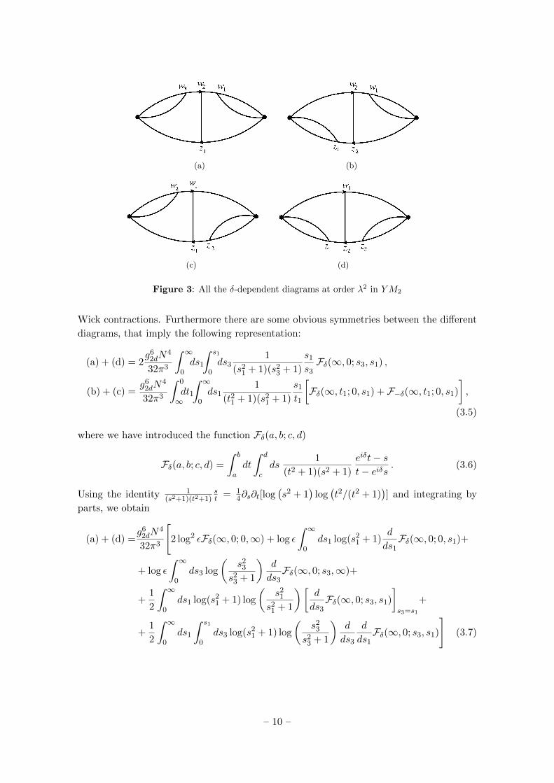
3.2 Operator insertions of length L = 1

The first non-trivial contribution in this case appears at order λ2: we need at least one

propagator connecting the two halves of the wedge, to carry the dependence on the opening

angle δ. Then we have to consider the effect of the operator insertions, which should be

connected to the contour, respecting planarity, in all possible ways. The relevant choices

are represented in Figure 3. We remark that every diagram has the same weight: in

fact the operator we study is single-trace and every diagram arises from an unique set of

– 9 –

(a) (b)

(c) (d)

Figure 3: All the δ-dependent diagrams at order λ2 in YM2

Wick contractions. Furthermore there are some obvious symmetries between the different

diagrams, that imply the following representation:

(a) + (d) = 2g6

2dN4

32π3

∫ ∞0ds1

∫ s1

0ds3

1

(s21 + 1)(s2

3 + 1)

s1

s3Fδ(∞, 0; s3, s1) ,

(b) + (c) =g6

2dN4

32π3

∫ 0

∞dt1

∫ ∞0ds1

1

(t21 + 1)(s21 + 1)

s1

t1

[Fδ(∞, t1; 0, s1) + F−δ(∞, t1; 0, s1)

],

(3.5)

where we have introduced the function Fδ(a, b; c, d)

Fδ(a, b; c, d) =

∫ b

adt

∫ d

cds

1

(t2 + 1)(s2 + 1)

eiδt− st− eiδs

. (3.6)

Using the identity 1(s2+1)(t2+1)

st = 1

4∂s∂t[log(s2 + 1

)log(t2/(t2 + 1)

)] and integrating by

parts, we obtain

(a) + (d) =g6

2dN4

32π3

[2 log2 εFδ(∞, 0; 0,∞) + log ε

∫ ∞0

ds1 log(s21 + 1)

d

ds1Fδ(∞, 0; 0, s1)+

+ log ε

∫ ∞0

ds3 log

(s2

3

s23 + 1

)d

ds3Fδ(∞, 0; s3,∞)+

+1

2

∫ ∞0

ds1 log(s21 + 1) log

(s2

1

s21 + 1

)[d

ds3Fδ(∞, 0; s3, s1)

]s3=s1

+

+1

2

∫ ∞0

ds1

∫ s1

0ds3 log(s2

1 + 1) log

(s2

3

s23 + 1

)d

ds3

d

ds1Fδ(∞, 0; s3, s1)

](3.7)

– 10 –

and

(b) + (c) =g6

2dN4

32π3

[− log2 ε

[Fδ(∞, 0; 0,∞) + F−δ(∞, 0; 0,∞)

]+

+1

2log ε

∫ 0

∞dt1 log

(t21

t21 + 1

)d

dt1

[Fδ(∞, t1; 0,∞) + F−δ(∞, t1; 0,∞)

]−

− 1

2log ε

∫ ∞0

ds1 log(s2

1 + 1) d

ds1

[Fδ(∞, 0; 0, s1) + F−δ(∞, 0; 0, s1)

]+ (3.8)

+1

4

∫ 0

∞dt1

∫ ∞0

ds1 log(s2

1 + 1)

log

(t21

t21 + 1

)d

dt1

d

ds1

[Fδ(∞, t1; 0, s1) + F−δ(∞, t1; 0, s1)

],

where ε is a regulator that cuts the contour in a neighborhood of the operator insertions

and it will be send to zero at the end of the computation. Now using that

d

daF±δ(a, 0; 0,∞) =

d

daF∓δ(∞, 0; 0, a) ,

d

daF±δ(∞, 0; a,∞) =

d

daF∓δ(∞, a; 0,∞) (3.9)

and the definition (2.19), we can sum up all the contributions in (3.7) and (3.8) obtaining

M(1)1 = −

g42dN

2

4π2

{1

2

∫ ∞0ds1 log(s2

1 + 1) log

(s2

1

s21 + 1

)[d

ds3Fδ(∞, 0; s3, s1)

]s3=s1

(3.10)

− 1

4

∫ ∞0dt1

∫ ∞0ds1 log

(s2

1 + 1)

log

(t21

t21 + 1

)d

dt1

d

ds1

[Fδ(∞, t1; 0, s1) + F−δ(∞, t1; 0, s1)

]},

where we have definedM(l)L as the sum of the δ-dependent part of 〈W(2d)

L (δ)〉 at loop order

l. To derive the above equation we have taken advantage of the useful relations

Fδ(∞, 0; 0,∞) = F−δ(∞, 0; 0,∞) ,d

da

d

dbF±δ(∞, 0; a, b) = 0 ,∫ ∞

0da log

(a2

a2 + 1

)d

daF±δ(∞, a; 0,∞) =

∫ ∞0

db log(b2 + 1

) ddbF±δ(∞, 0; 0, b) .

(3.11)

We remark that the dependence on the cutoff ε disappears: as expected we end up with

a finite result. We further observe that turning δ → −δ is the same as taking complex

conjugation, then we can rewrite (3.10) as follows

M(1)1 = −

g42dN

2

16π2

{∫ ∞0

ds1 log(s21 + 1) log

(s2

1

s21 + 1

)[d

ds3Fδ(∞, 0; s3, s1)

]s3=s1

−∫ ∞

0dt1

∫ ∞0

ds1 log(s2

1 + 1)

log

(t21

t21 + 1

)d

dt1

d

ds1Fδ(∞, t1; 0, s1)

}+c.c.

(3.12)

and performing the derivatives (3.12) becomes

M(1)1 = −

g42dN

2

16π2

∫ ∞0dsdt

log(s2 + 1)

(t2 + 1)(s2 + 1)

eiδt− st− eiδs

[log

(s2

s2 + 1

)− log

(t2

t2 + 1

)]+c.c.

(3.13)

– 11 –

The function H1 is then obtained with the help of (2.20), then at one-loop order we have

H(1)1 (λ, ϕ) =

1

2∂δM

(1)1

∣∣∣∣ δ=π−ϕg22d

=−2g2/A

. (3.14)

Exploiting the simple decomposition

eiδt− st− eiδs

= − ts

+1

s

s2 + 1

eiδs− t− 1

s

t2 + 1

eiδs− t, (3.15)

the derivative of (3.13) becomes

g42dN2

16π2

∫ ∞0

dsdtlog(s2 + 1)

s

[1

(t2 + 1)− 1

(s2 + 1)

][log

(s2

s2 + 1

)−log

(t2

t2 + 1

)]∂δ

(1

eiδs− t

)+c.c.

(3.16)

Using

∂δ

(1

eiδs− t

)= −is eiδ∂t

(1

eiδs− t

), (3.17)

the integral (3.16) takes the form:

ig42dN

2

16π2

∫ ∞0ds

{log(s2 + 1) log

(s2

s2 + 1

)s

s2 + 1− (3.18)

− 2

∫ ∞0dt

[log

(s2

s2 + 1

)t log(s2 + 1)

(t2 + 1)2

eiδ

eiδs− t− log

(t2

t2 + 1

)1− t2

1 + t2s

1 + s2

1

eiδs− t

]}+c.c.

Summing up the integrands with their complex conjugate (the first term vanishes) and

changing variables s→ √ωρ and t→√ω/ρ, we obtain:

∂δM(1)1 = −

g42dN

2

8π2

∫ ∞0dωdρ

sin δ [(ρ+ ω)(ρω − 1) + ρ(1 + ρω) log(1 + ρω)] log(

ρω1+ρω

)(1 + ρω)(ρ+ ω)2(ρ2 − 2ρ cos δ + 1)

=g4

2dN2

4π2sin δ

∫ ∞0dρ

log2 ρ

(ρ2 − 1)(ρ2 − 2ρ cos δ + 1). (3.19)

The integration domain is easily restricted to [0, 1] and we arrive at

∂δM(1)1 = −

g42dN

2

4π2sin δ

∫ 1

0dρ

log2 ρ

ρ2 − 2ρ cos δ + 1= −g4

2dN2 π

3B3

(δ

2π

), (3.20)

where the Bn(x) are the Bernoulli polynomials defined as

B2n+1(x) =(−1)n+12(2n+ 1) sin(2πx)

(2π)2n+1

∫ 1

0dt

log2n t

t2 − 2t cos(2πx) + 1. (3.21)

Finally, using (3.14), we find the desired result

H(1)1 (λ, ϕ) = − λ2

24πB3

(π − ϕ

2π

). (3.22)

– 12 –

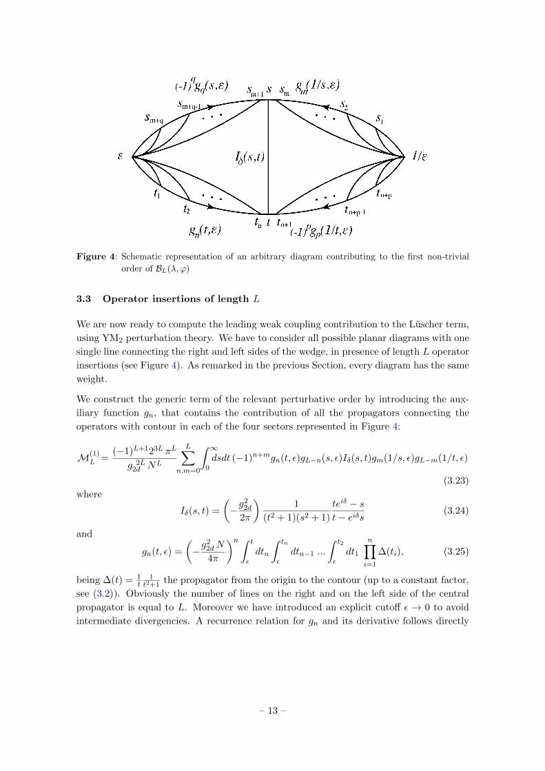
Figure 4: Schematic representation of an arbitrary diagram contributing to the first non-trivial

order of BL(λ, ϕ)

3.3 Operator insertions of length L

We are now ready to compute the leading weak coupling contribution to the Luscher term,

using YM2 perturbation theory. We have to consider all possible planar diagrams with one

single line connecting the right and left sides of the wedge, in presence of length L operator

insertions (see Figure 4). As remarked in the previous Section, every diagram has the same

weight.

We construct the generic term of the relevant perturbative order by introducing the aux-

iliary function gn, that contains the contribution of all the propagators connecting the

operators with contour in each of the four sectors represented in Figure 4:

M(1)L =

(−1)L+123L πL

g 2L2d NL

L∑n,m=0

∫ ∞0dsdt (−1)n+mgn(t, ε)gL−n(s, ε)Iδ(s, t)gm(1/s, ε)gL−m(1/t, ε)

(3.23)

where

Iδ(s, t) =

(−g2

2d

2π

)1

(t2 + 1)(s2 + 1)

teiδ − st− eiδs

(3.24)

and

gn(t, ε) =

(−g2

2dN

4π

)n ∫ t

εdtn

∫ tn

εdtn−1 ...

∫ t2

εdt1

n∏i=1

∆(ti), (3.25)

being ∆(t) = 1t

1t2+1

the propagator from the origin to the contour (up to a constant factor,

see (3.2)). Obviously the number of lines on the right and on the left side of the central

propagator is equal to L. Moreover we have introduced an explicit cutoff ε → 0 to avoid

intermediate divergencies. A recurrence relation for gn and its derivative follows directly

– 13 –

from its definition:

gn(t, ε) =

(−g2

2dN

4π

)∫ t

εdtn ∆(tn) gn−1(tn, ε) ,

d

dtgn(t, ε) =

(−g2

2dN

4π

)∆(t) gn−1(t, ε) .

(3.26)

As shown in the Appendix A, we can combine these two equations into a single recurrence

relation, involving just gn(t, ε)

gn(t, ε) = −n∑k=1

(−α)k

k!logk

(t2

t2 + 1

)gn−k(t, ε)− (t→ ε), (3.27)

where α = −g22dN8π . We can solve the recurrence relation by finding the related generating

function G(t, ε, z)

gn(t, ε) =1

2πi

∮γ

dz

zn+1G(t, ε, z) , (3.28)

for a suitable closed curve γ around the origin. We have obtained (see Appendix A for the

details)

G(t, ε, z) =

(t2

t2 + 1

ε2 + 1

ε2

)αz. (3.29)

Then (3.23) becomes

M(1)L =

(−1)L+1

(2πi)423L πL

g 2L2d NL

L∑n,m=0

∫ ∞0

dsdt

∮G(t, ε, z)

zn+1

G−1(s, ε, w)

wL−n+1Iδ(s, t)

G(1/s, ε, v)

vm+1

G−1(1/t, ε, u)

uL−m+1.

(3.30)

The sums over m and n are done explicitly

L∑n=0

1

zn+1wL−n+1=z−(L+1) − w−(L+1)

w − z(3.31)

and using the observations in Appendix A and in particular the formula (A.18), we obtain

M(1)L =

(−1)L+1

(2πi)223L πL

g 2L2d NL

(−g22d2π

)×

×∫ ∞0

dsdt

∮dz

zL+1

dv

vL+1

[(t2(1 + s2)

s2(1 + t2)

)αz((1 + t2)

(1 + s2)

)αv1

(t2 + 1)(s2 + 1)

teiδ − st− eiδs

].

(3.32)

Notice that the ε-dependence has disappeared: the cancellation of the intermediate diver-

gencies is a non-trivial bonus of our method.

Computing the residues, (3.32) takes the following compact form

M(1)L =

(−1)L+1α2L

(L!)2

23L πL

g 2L2d NL

(−g2

2d

2π

)∫ ∞0dsdt

[log(t2(1+s2)s2(1+t2)

)log(

(1+t2)(1+s2)

)]L(t2 + 1)(s2 + 1)

teiδ − st− eiδs

.

(3.33)

– 14 –

We are interested in calculating the Bremsstrahlung function, so we take the derivative of

the VEV of the Wilson loop as seen in the equation (2.6). Using (3.17), after some algebra,

we find

H(1)L = i

(−1)L+1α2L

2(L!)2

23L πL

g 2L2d NL

(−g2

2d

2π

)∫ ∞0dsdt

{[log

(t2(1 + s2)

s2(1 + t2)

)log

((1 + t2)

(1 + s2)

)]L×[

1

t2 + 1∂s

(1

eiδs− t

)+

eiδ

s2 + 1∂t

(1

eiδs− t

)]}∣∣∣∣ δ=π−ϕg22d

=−2g2/A

.

(3.34)

Performing some integration by parts and transformations s↔ t and s, t→ 1s,t , the change

of variables s→ √ωρ and t→√ω/ρ gives

H(1)L = −(−1)L+1α2L

L!(L− 1)!

23L πL

g 2L2d NL

(−g2

2d

2π

)sin δ (3.35)

×∫ 1

0dρ

∫ ∞0dω

[log

(ρ(ρ+ ω)

ρω + 1

)log

(ρ(ρω + 1)

ρ+ ω

)]L−1 (ρ2 − 1) log ρ

(ρ+ ω)(1 + ρω)(ρ2 − 2ρ cos δ + 1)

∣∣∣∣∣ δ=π−ϕg22d

=−2g2/A

.

Using the expansion[log

(ρ(ρ+ ω)

ρω + 1

)log

(ρ(ρω + 1)

ρ+ ω

)]L−1

=L−1∑k=0

(L− 1

k

)(−1)k log2(L−1−k) ρ log2k

(ρ+ ω

ρω + 1

),

(3.36)

the integration over ω is straightforward since

∫dω

log2k(ρ+ωρω+1

)(ρ+ ω)(1 + ρω)

= −log2k+1

(ρ+ωρω+1

)(ρ2 − 1)(2k + 1)

. (3.37)

Then we obtain

H(1)L = − (−1)L+1α2L

L!(L− 1)!

23L πL

g 2L2d NL

(−g22d2π

)β

(1

2, L

){sin δ

∫ 1

0

dρlog2L ρ

ρ2 − 2ρ cos δ + 1

}∣∣∣∣∣δ=π−ϕ

g22d

=−2g2/A

,

(3.38)

where β(a, b) is the Euler Beta function. The integral in (3.38) is basically the standard

representation (3.21) of the Bernoulli polynomials. Therefore H(1)L becomes:

H(1)L = −(−1)L+1α2L

L!(L− 1)!

23L πL

g 2L2d NL

(−g2

2d

2π

)β

(1

2, L

)(2π)2L+1(−1)L+1

2(2L+ 1)B2L+1

(π − ϕ

2π

).

(3.39)

Finally inserting the expression for α and using (2.3), we obtain the desired result

H(1)L = − (−1)LλL+1

4π(2L+ 1)!B2L+1

(π − ϕ

2π

). (3.40)

– 15 –

z

x2

x1

x

x

S

N

w

(a) H1

z x2

x1

x

x

S

N

w

(b) H2

z x2x1

x

x

S

N

(c) X1

z x2x1

x

x

S

N

(d) X2

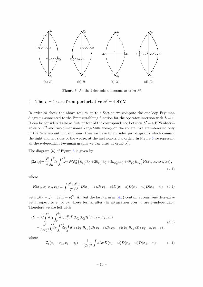
Figure 5: All the δ-dependent diagrams at order λ2

4 The L = 1 case from perturbative N = 4 SYM

In order to check the above results, in this Section we compute the one-loop Feynman

diagrams associated to the Bremsstrahlung function for the operator insertion with L = 1.

It can be considered also as further test of the correspondence between N = 4 BPS observ-

ables on S2 and two-dimensional Yang-Mills theory on the sphere. We are interested only

in the δ-dependent contributions, then we have to consider just diagrams which connect

the right and left sides of the wedge, at the first non-trivial order. In Figure 5 we represent

all the δ-dependent Feynman graphs we can draw at order λ2.

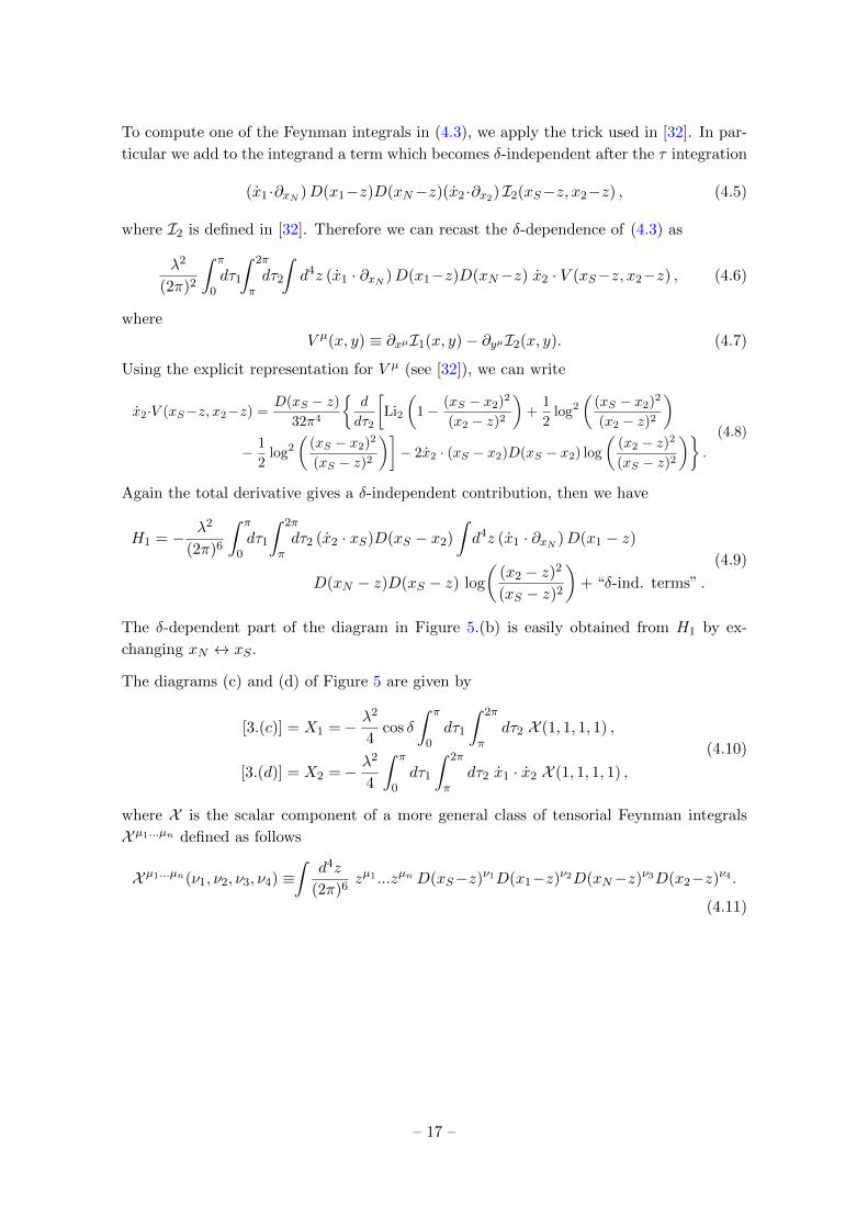
The diagram (a) of Figure 5 is given by

[3.(a)]=λ2

4

∫ π

0dτ1

∫ 2π

πdτ2 x

µ1 x

ν2

(∂xµ1 ∂x

ν2+2∂xµ1 ∂x

νS

+2∂xµN∂xν2 +4∂xµN

∂xνS

)H(x1, xN ;x2, xS) ,

(4.1)

where

H(x1, x2;x3, x4) ≡∫d4z d4w

(2π)8D(x1 − z)D(x2 − z)D(w − z)D(x3 − w)D(x4 − w) (4.2)

with D(x− y) = 1/(x− y)2. All but the last term in (4.1) contain at least one derivative

with respect to τ1 or τ2: these terms, after the integration over τ , are δ-independent.

Therefore we are left with

H1 = λ2

∫ π

0dτ1

∫ 2π

πdτ2 x

µ1 x

ν2 ∂xµN

∂xνSH(x1, xN ;x2, xS)

=λ2

(2π)2

∫ π

0dτ1

∫ 2π

πdτ2

∫d4z (x1 ·∂xN )D(x1−z)D(xN−z)(x2 ·∂xS ) I1(xS−z, x2−z) ,

(4.3)

where

I1(x1 − x3, x2 − x3) ≡ 1

(2π)6

∫d4wD(x1 − w)D(x2 − w)D(x3 − w) . (4.4)

– 16 –

To compute one of the Feynman integrals in (4.3), we apply the trick used in [32]. In par-

ticular we add to the integrand a term which becomes δ-independent after the τ integration

(x1 ·∂xN )D(x1−z)D(xN−z)(x2 ·∂x2) I2(xS−z, x2−z) , (4.5)

where I2 is defined in [32]. Therefore we can recast the δ-dependence of (4.3) as

λ2

(2π)2

∫ π

0dτ1

∫ 2π

πdτ2

∫d4z (x1 · ∂xN )D(x1−z)D(xN−z) x2 · V (xS−z, x2−z) , (4.6)

where

V µ(x, y) ≡ ∂xµI1(x, y)− ∂yµI2(x, y). (4.7)

Using the explicit representation for V µ (see [32]), we can write

x2·V (xS−z, x2−z) =D(xS − z)

32π4

{d

dτ2

[Li2

(1− (xS − x2)2

(x2 − z)2

)+

1

2log2

((xS − x2)2

(x2 − z)2

)− 1

2log2

((xS − x2)2

(xS − z)2

)]− 2x2 · (xS − x2)D(xS − x2) log

((x2 − z)2

(xS − z)2

)}.

(4.8)

Again the total derivative gives a δ-independent contribution, then we have

H1 = − λ2

(2π)6

∫ π

0dτ1

∫ 2π

πdτ2 (x2 · xS)D(xS − x2)

∫d4z (x1 · ∂xN )D(x1 − z)

D(xN − z)D(xS − z) log

((x2 − z)2

(xS − z)2

)+ “δ-ind. terms” .

(4.9)

The δ-dependent part of the diagram in Figure 5.(b) is easily obtained from H1 by ex-

changing xN ↔ xS .

The diagrams (c) and (d) of Figure 5 are given by

[3.(c)] = X1 =− λ2

4cos δ

∫ π

0dτ1

∫ 2π

πdτ2 X (1, 1, 1, 1) ,

[3.(d)] = X2 =− λ2

4

∫ π

0dτ1

∫ 2π

πdτ2 x1 · x2 X (1, 1, 1, 1) ,

(4.10)

where X is the scalar component of a more general class of tensorial Feynman integrals

X µ1...µn defined as follows

X µ1...µn(ν1, ν2, ν3, ν4) ≡∫

d4z

(2π)6zµ1 ...zµn D(xS−z)ν1D(x1−z)ν2D(xN−z)ν3D(x2−z)ν4 .

(4.11)

– 17 –

Now, recalling the definition (2.14) and denoting with the prime the derivative respect to

δ (notice that x2, x′2 and x2 form an orthogonal basis), we have

H ′1 =4λ2

∫ π

0dτ1

∫ 2π

πdτ2 (x2 · xS)D(xS − x2)x′µ2 xν1 (xνNX µ(1, 1, 2, 1)−X µν(1, 1, 2, 1)) ,

H ′2 =4λ2

∫ π

0dτ1

∫ 2π

πdτ2 (x2 · xN )D(xN − x2)x′µ2 xν1 (xνSX µ(2, 1, 1, 1)−X µν(2, 1, 1, 1)) ,

X ′1 =λ2

4

∫ π

0dτ1

∫ 2π

πdτ2

(sin δX (1, 1, 1, 1)− 2 cos δ x′µ2 X

µ(1, 1, 1, 2)),

X ′2 =λ2

4

∫ π

0dτ1

∫ 2π

πdτ2

(−(x1 · x′2)X (1, 1, 1, 1) + 2(x1 · x2)x′µ2 X

µ(1, 1, 1, 2)).

(4.12)

Finally, summing up all the different contributions in N = 4 SYM, we obtain the function

H(1)1 defined in (2.14)

H(1)1 =

1

2(H ′1 +H ′2 +X ′1 +X ′2)

∣∣∣∣δ=π−ϕ

. (4.13)

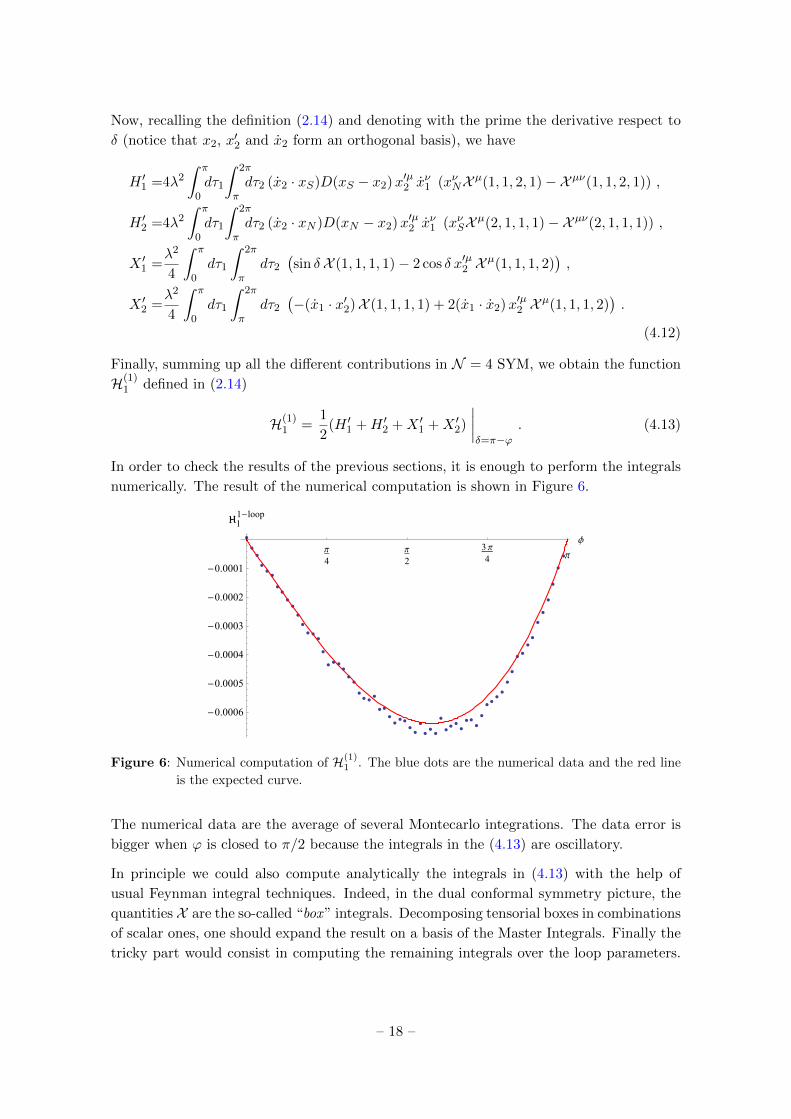
In order to check the results of the previous sections, it is enough to perform the integrals

numerically. The result of the numerical computation is shown in Figure 6.

Π4

Π2

3 Π4 Π

Φ

-0.0006

-0.0005

-0.0004

-0.0003

-0.0002

-0.0001

H11-loop

Figure 6: Numerical computation of H(1)1 . The blue dots are the numerical data and the red line

is the expected curve.

The numerical data are the average of several Montecarlo integrations. The data error is

bigger when ϕ is closed to π/2 because the integrals in the (4.13) are oscillatory.

In principle we could also compute analytically the integrals in (4.13) with the help of

usual Feynman integral techniques. Indeed, in the dual conformal symmetry picture, the

quantities X are the so-called “box” integrals. Decomposing tensorial boxes in combinations

of scalar ones, one should expand the result on a basis of the Master Integrals. Finally the

tricky part would consist in computing the remaining integrals over the loop parameters.

– 18 –

These quite technical computations are beyond the aim of this paper and we leave them

to further developments in a may be more general setting.

5 Conclusions and outlook

In this paper we have explored the possibility to study the near-BPS expansion of the

generalized cusp anomalous dimension with L units of R-charge by means of supersym-

metric localization. The R-charge is provided by the insertion certain scalar operators

into a cusped Wilson loop, according to the original proposal of [21], [22]. The relevant

generalized Bremsstrahlung function BL(λ, ϕ) has been computed by solving a set of TBA

equations in the near-BPS limit [27, 28] and, more recently, using QSC approach [24]. We

have proposed here a generalization of the method discussed in [25], relating the computa-

tion to the quantum average of some BPS Wilson loops with local operator insertions along

the contour. The system should localize into perturbative YM2 on S2, in the zero-instanton

sector, suggesting the possibility to perform exact calculations in this framework. We have

checked our proposal, reproducing the leading Luscher correction at weak coupling to the

generalized cusp anomalous dimension. We have further tested our strategy in the case

L = 1, using Feynman diagrams directly in N = 4 Super Yang-Mills theory.

Our investigations represent only a first step in connecting integrability results with local-

ization outputs: we certainly would like to derive the complete expression for BL(λ, ϕ) in

this framework. Two-dimensional Yang-Mills theory on the sphere has an exact solution,

even at finite N [39, 40]: on the other hand, the construction of the vacuum expectation

values of Wilson loops with local operator insertions has not been studied in the past, at

least to our knowledge. The matrix model [29], computing the generalized Bremsstrahlung

function, strongly suggests that these two-dimensional observables, in the zero-instanton

sector, should be obtained by extending the techniques of [14]. One could expect that also

a finite N answer is possible, as in the case of L = 0. We are currently working on these

topics and we hope to report some progress soon.

A further direction could be to develop an efficient technique to explore this kind of ob-

servable directly in four-dimensions, by using perturbation theory. It would be interesting

to go beyond the near-BPS case and to study the anomalous dimensions for more general

local operator insertions4. The construction of similar systems in three-dimensional ABJM

theory should also be feasible and could provide new insights to get exact results.

Acknowledgements

We warmly thank N. Drukker and S. Giombi for discussions and suggestions. One of

us (M.P.) would like to thank to the Group ”Gauge fields from strings” at Humboldt

University for the warm hospitality while this work has been completed. This work has

4We thank Nadav Drukker for suggesting us these possibilities.

– 19 –

been supported in part by MIUR, INFN and MPNS-COST Action MP1210 “The String

Theory Universe”.

Appendix

A The generating function G(t, ε, z) and some related properties

We present here the derivation of some results that have been used in computing the

Luscher term from YM2 perturbation theory: in particular we will examine the derivation

of the generating function G(t, ε, z). We start from the two relations (3.26)

gn(t, ε) =

(−g2

2dN

4π

)∫ t

εdtn ∆(tn) gn−1(tn, ε) , (A.1)

d

dtgn(t, ε) =

(−g2

2dN

4π

)∆(t) gn−1(t, ε) (A.2)

with g0(t, ε) = 1. Using the identity

∆(t) =1

2

d

dtlog

(t2

t2 + 1

)(A.3)

into the recurrence relation (A.1) and integrating by parts we obtain

gn(t, ε) =

(−g2

2dN

8π

){log

(t2

t2 + 1

)gn−1(t, ε)− log

(ε2

ε2 + 1

)gn−1(ε, ε)−

−∫ t

εdtn log

(t2n

t2n + 1

)d

dtngn−1(tn, ε)

}

=

(−g2

2dN

8π

){log

(t2

t2 + 1

)gn−1(t, ε)− log

(ε2

ε2 + 1

)gn−1(ε, ε)−

−(−g2

2dN

4π

)∫ t

εdtn log

(t2n

t2n + 1

)∆(tn) gn−2(tn, ε)

}.

(A.4)

We rewrite the product in the last line as

log

(t2n

t2n + 1

)∆(tn) =

1

4

d

dtnlog2

(t2n

t2n + 1

)(A.5)

and integrating by parts again we obtain

gn(t, ε) =

{[(−g2

2dN

8π

)log

(t2

t2 + 1

)gn−1(t, ε)− 1

2

(−g2

2dN

8π

)2

log2

(t2

t2 + 1

)gn−2(t, ε)

− (t→ ε)

]+

1

2

(−g2

2dN

8π

)2 ∫ t

εdtn log2

(t2n

t2n + 1

)d

dtngn−2(tn, ε)

}. (A.6)

– 20 –

The procedure can be iterated n− 1 times and, defining α = −g22dN8π , we arrive at

gn(t, ε) = −n∑k=1

(−α)k

k!logk

(t2

t2 + 1

)gn−k(t, ε)− (t→ ε) . (A.7)

We can solve the recurrence by finding the generating function: given the sequence gn(t, ε)

we define

G(t, ε, z) =∞∑n=0

gn(t, ε) zn with z ∈ C , (A.8)

then using Cauchy’s formula

gn(t, ε) =1

2πi

∮γ

dz

zn+1G(t, ε, z) (A.9)

with γ a closed curve around the origin.

Going back to the equation (A.7), we notice that gn−k(ε, ε) = 0 for k 6= n. Then we get:

G(t, ε, z)− 1 =

∞∑n=1

gn(t, ε)zn = −∞∑n=1

znn∑k=1

(−α)k

k!logk

(t2

t2 + 1

)gn−k(t, ε)+

+∞∑n=1

(−αz)n

n!logn

(ε2

ε2 + 1

)

=−∞∑k=1

zk(−α)k

k!logk

(t2

t2 + 1

) ∞∑n=k

gn−k(t, ε)zn−k + e

−αz log(

ε2

ε2+1

)− 1

=−(e−αz log

(t2

t2+1

)− 1

)G(t, ε, z) + e

−αz log(

ε2

ε2+1

)− 1 . (A.10)

Finally the generating function is:

G(t, ε, z) =

(t2

t2 + 1

ε2 + 1

ε2

)αz. (A.11)

Following the same steps, we can find that the generating function associated to the se-

quence (−1)ngn(s, ε) is G−1(s, ε, w).

Let us now consider the expression (3.30) and (3.31): we have to evaluate a double-integral

of the following type

A ≡ 1

(2πi)2

∮dzdw

z−(L+1) − w−(L+1)

w − zF (z, w) (A.12)

with F (z, w) analytic around z, w = 0 and symmetric in w ↔ z

F (z, w) =∞∑n=0

∞∑m=0

an,mznwm , (A.13)

where an,m = am,n. Redefining z → zw we have

A =1

(2πi)2

∮dzdw

1

wL+1

z−(L+1) − 1

1− z

∞∑m,n=0

an,mznwn+m . (A.14)

– 21 –

Performing the integral over w, we obtain

A =1

(2πi)

L∑n=0

an,L−n

∮dz

zL+1−n1− zL+1

1− z=

L∑n=0

an,L−n . (A.15)

Notice that the function F (w, z) at w = z has the form

F (z, z) =

∞∑n=0

∞∑m=0

an,mzn+m =

∞∑k=0

bkzk (A.16)

whit bk =∑k

n=0 an,k−n. Then

A = bL =1

2πi

∮dz

zL+1F (z, z), (A.17)

i.e. ∮dzdw

z−(L+1) − w−(L+1)

w − zF (z, w) = 2πi

∮dz

zL+1F (z, z) . (A.18)

References

[1] N. Beisert et al., “Review of AdS/CFT Integrability: An Overview,” Lett. Math. Phys. 99

(2012) 3 [arXiv:1012.3982 [hep-th]].

[2] V. Pestun, “Localization of gauge theory on a four-sphere and supersymmetric Wilson loops,”

Commun. Math. Phys. 313 (2012) 71 [arXiv:0712.2824 [hep-th]].

[3] G. Arutyunov and S. Frolov, “String hypothesis for the AdS5 × S5 mirror,” JHEP 0903

(2009) 152 [arXiv:0901.1417 [hep-th]].

[4] G. Arutyunov and S. Frolov, “Thermodynamic Bethe Ansatz for the AdS5 × S5 Mirror

Model,” JHEP 0905 (2009) 068 [arXiv:0903.0141 [hep-th]].

[5] N. Gromov, V. Kazakov and P. Vieira, “Exact Spectrum of Anomalous Dimensions of Planar

N = 4 Supersymmetric Yang-Mills Theory,” Phys. Rev. Lett. 103 (2009) 131601

[arXiv:0901.3753 [hep-th]].

[6] D. Bombardelli, D. Fioravanti and R. Tateo, “Thermodynamic Bethe Ansatz for planar

AdS/CFT: A Proposal,” J. Phys. A 42 (2009) 375401 [arXiv:0902.3930 [hep-th]].

[7] N. Gromov, V. Kazakov, S. Leurent and D. Volin, “Quantum Spectral Curve for Planar

N = 4 Super-Yang-Mills Theory,” Phys. Rev. Lett. 112 (2014) 1, 011602 [arXiv:1305.1939

[hep-th]].

[8] J. K. Erickson, G. W. Semenoff and K. Zarembo, “Wilson loops in N = 4 supersymmetric

Yang-Mills theory,” Nucl. Phys. B 582 (2000) 155 [hep-th/0003055].

[9] N. Drukker and D. J. Gross, “An Exact prediction of N = 4 SUSYM theory for string

theory,” J. Math. Phys. 42, 2896 (2001) [hep-th/0010274].

[10] N. Drukker, “1/4 BPS circular loops, unstable world-sheet instantons and the matrix model,”

JHEP 0609, 004 (2006) [hep-th/0605151].

[11] N. Drukker, S. Giombi, R. Ricci and D. Trancanelli, “More supersymmetric Wilson loops,”

Phys. Rev. D 76 (2007) 107703 [arXiv:0704.2237 [hep-th]].

– 22 –

[12] N. Drukker, S. Giombi, R. Ricci and D. Trancanelli, “Supersymmetric Wilson loops on S3,”

JHEP 0805 (2008) 017 [arXiv:0711.3226 [hep-th]].

[13] V. Pestun, “Localization of the four-dimensional N = 4 SYM to a two-sphere and 1/8 BPS

Wilson loops”, JHEP 1212 (2012) 067, [arXiv:0906.0638 [hep-th]].

[14] S. Giombi and V. Pestun, “Correlators of Wilson loops and local operators from multi-matrix

models and strings in AdS”, JHEP 1301 (2013) 101, [arXiv:1207.7083 [hep-th]].

[15] S. Giombi and V. Pestun, “Correlators of local operators and 1/8 BPS Wilson loops on S**2

from 2d YM and matrix models”, JHEP 1010 (2010) 033, [arXiv:0906.1572 [hep-th]].

[16] A. M. Polyakov, “Gauge Fields as Rings of Glue,” Nucl. Phys. B 164 (1980) 171.

[17] G. P. Korchemsky and A. V. Radyushkin, “Renormalization of the Wilson Loops Beyond the

Leading Order,” Nucl. Phys. B 283 (1987) 342.

[18] N. Beisert, B. Eden and M. Staudacher, “Transcendentality and Crossing,” J. Stat. Mech.

0701 (2007) P01021 [hep-th/0610251].

[19] Z. Bern, M. Czakon, L. J. Dixon, D. A. Kosower and V. A. Smirnov, “The Four-Loop Planar

Amplitude and Cusp Anomalous Dimension in Maximally Supersymmetric Yang-Mills

Theory,” Phys. Rev. D 75 (2007) 085010 [hep-th/0610248].

[20] S. S. Gubser, I. R. Klebanov and A. M. Polyakov, “A Semiclassical limit of the gauge/string

correspondence,” Nucl. Phys. B 636 (2002) 99 [hep-th/0204051].

[21] D. Correa, J. Maldacena and A. Sever, “The quark anti-quark potential and the cusp

anomalous dimension from a TBA equation,” JHEP 1208, 134 (2012) [arXiv:1203.1913

[hep-th]].

[22] N. Drukker, “Integrable Wilson loops,” JHEP 1310, 135 (2013) [arXiv:1203.1617 [hep-th]].

[23] N. Drukker and V. Forini, “Generalized quark-antiquark potential at weak and strong

coupling,” JHEP 1106, 131 (2011) [arXiv:1105.5144 [hep-th]].

[24] N. Gromov and F. Levkovich-Maslyuk, “Quantum Spectral Curve for a Cusped Wilson Line

in N = 4 SYM,” arXiv:1510.02098 [hep-th].

[25] D. Correa, J. Henn, J. Maldacena and A. Sever, “An exact formula for the radiation of a

moving quark in N = 4 Super Yang Mills,” JHEP 1206 (2012) 048 [arXiv:1202.4455

[hep-th]].

[26] B. Fiol, B. Garolera and A. Lewkowycz, “Exact results for static and radiative fields of a

quark in N = 4 Super Yang-Mills,” JHEP 1205 (2012) 093 [arXiv:1202.5292 [hep-th]].

[27] N. Gromov and A. Sever, “Analytic Solution of Bremsstrahlung TBA,” JHEP 1211 (2012)

075 [arXiv:1207.5489 [hep-th]].

[28] N. Gromov, F. Levkovich-Maslyuk and G. Sizov, “Analytic Solution of Bremsstrahlung TBA

II: Turning on the Sphere Angle,” JHEP 1310 (2013) 036 [arXiv:1305.1944 [hep-th]].

[29] G. Sizov and S. Valatka, “Algebraic Curve for a Cusped Wilson Line,” JHEP 1405 (2014)

149 [arXiv:1306.2527 [hep-th]].

[30] N. Drukker and J. Plefka, “Superprotected n-point correlation functions of local operators in

N = 4 super Yang-Mills”, JHEP 0904 (2009) 052, [arXiv:0901.3653 [hep-th]].

[31] S. Giombi, V. Pestun and R. Ricci, “Notes on supersymmetric Wilson loops on a

two-sphere”, JHEP 1007 (2010) 088, [arXiv:0905.0665 [hep-th]].

– 23 –

[32] A. Bassetto, L. Griguolo, F. Pucci and D. Seminara, “Supersymmetric Wilson loops at two

loops”, JHEP 0806 (2008) 083, [arXiv:0804.3973 [hep-th]].

[33] D. Young, “BPS Wilson Loops on S2 at Higher Loops”, JHEP 0805 (2008) 077,

[arXiv:0804.4098 [hep-th]].

[34] A. Bassetto, L. Griguolo, F. Pucci, D. Seminara, S. Thambyahpillai and D. Young,

“Correlators of supersymmetric Wilson-loops, protected operators and matrix models in

N = 4 SYM ”, JHEP 0908 (2009) 061, [arXiv:0905.1943 [hep-th]].

[35] A. Bassetto, L. Griguolo, F. Pucci, D. Seminara, S. Thambyahpillai and D. Young,

“Correlators of supersymmetric Wilson loops at weak and strong coupling”, JHEP 1003

(2010) 038, [arXiv:0912.5440 [hep-th]].

[36] M. Bonini, L. Griguolo and M. Preti, “Correlators of chiral primaries and 1/8 BPS Wilson

loops from perturbation theory,” JHEP 1409, 083 (2014) [arXiv:1405.2895 [hep-th]].

[37] D. Correa, J. Henn, J. Maldacena and A. Sever, “The cusp anomalous dimension at three

loops and beyond,” JHEP 1205 (2012) 098 [arXiv:1203.1019 [hep-th]].

[38] K. Zarembo, “Supersymmetric Wilson loops,” Nucl. Phys. B 643 (2002) 157

[hep-th/0205160].

[39] A. A. Migdal, “Gauge Transitions in Gauge and Spin Lattice Systems”, Sov.Phys.JETP 42

(1975) 743, [Zh.Eksp.Teor.Fiz. 69 (1975) 1457].

[40] E. Witten, “On quantum gauge theories in two-dimensions”, Commun.Math.Phys. 141

(1991) 153-209.

– 24 –