breeding population density and habitat use of …

BREEDING POPULATION DENSITY AND HABITAT USE OF

SWAINSON’S WARBLERS IN A GEORGIA FLOODPLAIN FOREST

by

ELIZABETH ANN WRIGHT

(Under the direction of J. Michael Meyers and Robert J. Warren)

ABSTRACT

I examined density and habitat use of a Swainson’s Warbler (Limnothlypisswainsonii) breeding population in Georgia. This songbird species is inadequatelymonitored, and may be declining due to anthropogenic alteration of floodplain forestbreeding habitats. I used distance sampling methods to estimate density, finding 9.4singing males/ha (CV = 0.298). Individuals were encountered too infrequently toproduce a low-variance estimate, and distance sampling thus may be impracticable formonitoring this relatively rare species. I developed a set of multivariate habitat modelsusing binary logistic regression techniques, based on measurement of 22 variables in 56plots occupied by Swainson’s Warblers and 110 unoccupied plots. Occupied areas werecharacterized by high stem density of cane (Arundinaria gigantea) and other shrub layervegetation, and presence of abundant and accessible leaf litter. I recommend twohabitat models, which correctly classified 87-89% of plots in cross-validation runs, forpotential use in habitat assessment at other locations.

INDEX WORDS: Neotropical migrant, Bird, Songbird, Avian, Swainson’s Warbler,Limnothlypis swainsonii, Bond Swamp National Wildlife Refuge,Ocmulgee River, Georgia, Bottomland forest, Floodplain, Naturaldisturbance, Cane, Canebrake, Arundinaria gigantea, Populationdensity, Distance sampling, Bird survey methods, Habitat use, Habitatmodels, Logistic regression



by


B.A., Wells College, 1981

A Thesis Submitted to the Graduate Faculty of The University of Georgia

in Partial Fulfillment of the Requirements for the Degree

MASTER OF SCIENCE

ATHENS, GEORGIA

2002

© 2002

Elizabeth Ann Wright

All Rights Reserved



by


Major Professors: J. Michael MeyersRobert J. Warren

Committee: Robert J. CooperJ. Whitfield Gibbons

Electronic Version Approved:

Maureen GrassoDean of the Graduate SchoolThe University of GeorgiaDecember 2002

DEDICATION

To my father, Dr. Malcolm R. Wright;

In remembrance of my mother and my aunt,Mary Louise Waters Wright and Catherine Anne Waters Eschbach;

And for all those beings I’ve encountered along the way who inspired me with their passion, beauty, and imagination.

Disillusionment of Ten O’Clock

The houses are hauntedBy white night-gowns.None are green,Or purple with green rings,Or green with yellow rings,Or yellow with blue rings.None of them are strange,With socks of laceAnd beaded ceintures.People are not goingTo dream of baboons and periwinkles.Only, here and there, an old sailor,Drunk and asleep in his boots,Catches tigersIn red weather.

– Wallace Stevens

Emancipate yourself from mental slaveryNone but ourselves can free our minds.

– Robert Nestor Marley

iv

ACKNOWLEDGMENTS

Many people and institutions have contributed to the success of my research and

imminent completion of my degree. First, I thank my co-major professors: Joe Meyers,

who allowed me to work with songbirds despite my lack of experience, provided

extensive guidance, and secured project funding and materials; and Bob Warren, who

offered praise and encouragement at every turn. Both graciously withstood my

perfectionist-procrastinator tendencies. I also appreciate the contributions of my

advisory committee, especially: Bob Cooper for countless mind-opening discussions,

Whit Gibbons for twice showing up with live herps just when I needed a dose of the non-

human world, and both for reviewing my thesis with record speed. My faculty advisors

have demonstrated remarkable knowledge, wisdom, good humor, and generosity.

My studies would not have been possible without financial and in-kind support

from The University of Georgia’s Warnell School of Forest Resources, USGS Patuxent

Wildlife Research Center, U.S. Fish and Wildlife Service, and Georgia Ornithological

Society. Individuals deserving specific plaudits include: Bonnie Fancher for cheerful

assistance with data management and project paperwork; Clint Moore for modeling

advice and terrific SAS macros; Kristin Owens for field assistance under often difficult

conditions; Ronnie Shell and Carolyn Johnson for extensive logistical support; Chuck

and Rose Lane Leavell for the best field housing imaginable; Dan Markewitz and Martha

Campbell for soil sampling advice; and Lee Ashley for kindly storing my soil samples.

Others too numerous to list – my family, longtime friends, and those I’ve had the

pleasure of knowing during my Georgia sojourn – have taught me much, shared both

splendid and sobering experiences, and helped maintain my balance in myriad ways.

v

TABLE OF CONTENTS

Page

LIST OF TABLES . . . . . . . . . . . . . . . . . . . . . . . . . . . . . . . . . . . . . . . . . . . . . . . . . . . . viii

LIST OF FIGURES . . . . . . . . . . . . . . . . . . . . . . . . . . . . . . . . . . . . . . . . . . . . . . . . . . . ix

CHAPTERS:

1 INTRODUCTION . . . . . . . . . . . . . . . . . . . . . . . . . . . . . . . . . . . . . . . . . . . . . . . . 1

Swainson’s Warbler . . . . . . . . . . . . . . . . . . . . . . . . . . . . . . . . . . . . . . . . . . . . . . 3

Bird Survey Methods . . . . . . . . . . . . . . . . . . . . . . . . . . . . . . . . . . . . . . . . . . . . . 6

Southeastern Floodplain Forests . . . . . . . . . . . . . . . . . . . . . . . . . . . . . . . . . . . . 8

Previous Habitat Studies . . . . . . . . . . . . . . . . . . . . . . . . . . . . . . . . . . . . . . . . . 11

Study Area . . . . . . . . . . . . . . . . . . . . . . . . . . . . . . . . . . . . . . . . . . . . . . . . . . . . 16

Research Objectives . . . . . . . . . . . . . . . . . . . . . . . . . . . . . . . . . . . . . . . . . . . . 21

Literature Cited . . . . . . . . . . . . . . . . . . . . . . . . . . . . . . . . . . . . . . . . . . . . . . . . 21

2 ESTIMATING DENSITY OF A SWAINSON’S WARBLER BREEDING

POPULATION WITH DISTANCE SAMPLING . . . . . . . . . . . . . . . . . . . . . . . . . 31

Abstract . . . . . . . . . . . . . . . . . . . . . . . . . . . . . . . . . . . . . . . . . . . . . . . . . . . . . . 32

Introduction . . . . . . . . . . . . . . . . . . . . . . . . . . . . . . . . . . . . . . . . . . . . . . . . . . . 33

Study Area . . . . . . . . . . . . . . . . . . . . . . . . . . . . . . . . . . . . . . . . . . . . . . . . . . . . 35

Methods . . . . . . . . . . . . . . . . . . . . . . . . . . . . . . . . . . . . . . . . . . . . . . . . . . . . . 36

Results . . . . . . . . . . . . . . . . . . . . . . . . . . . . . . . . . . . . . . . . . . . . . . . . . . . . . . 39

Discussion . . . . . . . . . . . . . . . . . . . . . . . . . . . . . . . . . . . . . . . . . . . . . . . . . . . . 41

Acknowledgments . . . . . . . . . . . . . . . . . . . . . . . . . . . . . . . . . . . . . . . . . . . . . . 44


vi

3 MANAGEMENT MODELS FOR SWAINSON’S WARBLER BREEDING

HABITAT IN A GEORGIA FLOODPLAIN FOREST . . . . . . . . . . . . . . . . . . . . 50

Abstract . . . . . . . . . . . . . . . . . . . . . . . . . . . . . . . . . . . . . . . . . . . . . . . . . . . . . . 51

Introduction . . . . . . . . . . . . . . . . . . . . . . . . . . . . . . . . . . . . . . . . . . . . . . . . . . . 52

Study Area . . . . . . . . . . . . . . . . . . . . . . . . . . . . . . . . . . . . . . . . . . . . . . . . . . . . 54

Methods . . . . . . . . . . . . . . . . . . . . . . . . . . . . . . . . . . . . . . . . . . . . . . . . . . . . . 56

Results . . . . . . . . . . . . . . . . . . . . . . . . . . . . . . . . . . . . . . . . . . . . . . . . . . . . . . 61

Discussion . . . . . . . . . . . . . . . . . . . . . . . . . . . . . . . . . . . . . . . . . . . . . . . . . . . . 65

Management Implications . . . . . . . . . . . . . . . . . . . . . . . . . . . . . . . . . . . . . . . . 72

Acknowledgments . . . . . . . . . . . . . . . . . . . . . . . . . . . . . . . . . . . . . . . . . . . . . . 76


Appendix: Use of Habitat Models . . . . . . . . . . . . . . . . . . . . . . . . . . . . . . . . . . 83

4 SUMMARY AND CONCLUSIONS . . . . . . . . . . . . . . . . . . . . . . . . . . . . . . . . . . 86

vii

LIST OF TABLES

Page

Table 1. Wilcoxon rank-sum tests of habitat variables measured in plots occupied

versus unoccupied by Swainson’s Warblers at Bond Swamp National

Wildlife Refuge, Georgia, during the 2001 breeding season . . . . . . . . . . . 62

Table 2. Binary logistic regression models of habitat characteristics predicting

Swainson’s Warbler occupancy (singing males) at Bond Swamp National

Wildlife Refuge, Georgia, in 2001: top-ranked one- to six-variable models,

plus second-ranked three-variable model, based on AICc scores . . . . . . . 64

viii

LIST OF FIGURES

Page

Figure 1. Swainson’s Warbler male in territorial defense posture, as depicted by S. A.

Briggs (in Meanley 1971) . . . . . . . . . . . . . . . . . . . . . . . . . . . . . . . . . . . . . . . 4

Figure 2. U.S. Fish and Wildlife Service map of Bond Swamp National Wildlife

Refuge, Georgia . . . . . . . . . . . . . . . . . . . . . . . . . . . . . . . . . . . . . . . . . . . . 17

Figure 3. Topographic map of Bond Swamp National Wildlife Refuge and vicinity,

Georgia, adapted from U.S. Geological Survey Macon East quadrangle

1:24,000 scale topographic map (1981). . . . . . . . . . . . . . . . . . . . . . . . . . . 18

Figure 4. Swainson’s Warbler detections in transect surveys at Bond Swamp

National Wildlife Refuge, Georgia, 31 May-20 June 2001; detection

distances grouped into 30-m intervals (cutpoint is interval upper bound) . . 38

Figure 5. Sample scatterplot map of Swainson’s Warbler GPS locations; outlined

square indicates 50 m x 50 m area with greatest number of detections,

used as habitat plot location. . . . . . . . . . . . . . . . . . . . . . . . . . . . . . . . . . . 58

ix

Chapter I

INTRODUCTION

The canebrakes stretch along the slight rises of ground, often extendingfor miles, forming one of the most striking and interesting features of thecountry. They choke out other growths, the feathery, graceful canesstanding in ranks, tall, slender, serried, each but a few inches from hisbrother, and springing to a height of fifteen or twenty feet. They look likebamboos; they are well-nigh impenetrable to a man on horseback; evenon foot they make difficult walking unless free use is made of the heavybush-knife. It is impossible to see through them for more than fifteen ortwenty paces, and often for not half that distance. Bears make their lairsin them, and they are the refuge for hunted things.

– Excerpt from Theodore Roosevelt, “In the Louisiana Canebrakes” (1908)

Anthropogenic alteration of habitats used by Nearctic-Neotropical migratory birds

during the various phases of their annual cycle has been implicated as a principal cause

of population declines observed in many species (Terborgh 1989, Lovejoy 1992,

Robbins et al. 1993, Peterjohn et al. 1995, Askins 2000, Pashley et al. 2000). Although

ornithologists for several decades have debated the relative conservation importance of

habitats used by Nearctic-Neotropical migrants for breeding, overwintering, and

migration, an integrated view is emerging (Martin 1992, Terborgh 1989, Sherry and

Holmes 1995, Holmes and Sherry 2001). Recent research provides evidence that

events occurring during each discrete phase of the annual cycle can directly influence

other phases in substantive ways (Marra 1998). Thus, an “all-season” approach to

habitat conservation for Nearctic-Neotropical migrants may be warranted.

Literally dozens of studies have examined habitat selection and use by avian

species, but no single theory appears to have been widely accepted. Habitat selection –

i.e., the behavioral and psychological mechanisms by which birds or other animals

2

determine which areas to occupy and use during various parts of their annual and life

cycles – may be influenced in birds by a number of interacting ecological processes and

environmental factors operating at multiple scales (Lack 1933, Cody 1985). Settlement

of individuals in a given habitat may not reflect a conscious decision-making process but

rather a programmed response, established genetically or during the nestling/fledgling

stage, involving recognition of the features of a particular habitat type in which the

individual was successfully reared, the so-called “niche gestalt” (James 1971). Habitat

selection may reflect processes such as intra- and interspecific competition, as

evidenced by individual and social behaviors such as territoriality and density-dependent

habitat use (Grinnell 1917, Fretwell and Lucas 1969, Martin 1998), along with the

apparent selection of habitats to avoid predation (Martin 1998) and competition for

localized resources such as food and nest sites (Grinnell 1917, Gill 1995).

Environmental features that appear to influence habitat selection at various scales

include structure and species composition of vegetation (Lack 1933, MacArthur and

MacArthur 1961, James 1971, Holmes and Robinson 1981, Rotenberry 1985), climate

(Grinnell 1917), topography (Johnston and Odum 1956), hydrology and soils (Grinnell

1917), presence of ecological edges (Grinnell 1917, Johnston and Odum 1956), habitat

heterogeneity (Cody 1985, Robbins et al. 1989), and overall area of intact

(unfragmented) habitat available (Robbins et al. 1989). Individual birds may engage in a

hierarchical process (Johnson 1980) in which visible features of the landscape, such as

vegetation structure and topography, are used as “proximate cues” to gauge whether

specific habitats – from landscape to microsite scales – can provide those factors

ultimately needed for survival and reproduction, such as sufficient food, mating

opportunities, secure nest sites, and protection from predators, parasites, and

3

meteorological conditions (Lack 1933, James 1971, Anderson and Shugart 1974,

Johnson 1980, Robinson and Holmes 1984, Cody 1985, Martin 1998).

Availability and selection of suitable habitats may be especially critical for

Nearctic-Neotropical migratory birds given their extreme mobility and consequent need

to locate fitness-maximizing habitats several times each year (Cody 1985).

Understanding habitat selection and use thus is an essential element in conservation

efforts for Nearctic-Neotropical migrants, yet adequate information is lacking for many

species (Martin 1992, Finch and Stangel 1993, Askins 2000).

Loss of appropriate natural habitats as the result of human activities apparently

has not affected all Nearctic-Neotropical migratory bird species and groups equally.

This may be because the extent and intensity of anthropogenic disturbance has been

greater in habitat types most desirable for human use, such as those best-suited for

agriculture, timber harvest, or silviculture (Askins 2000, Brawn et al. 2001). Conversely,

certain habitat types have been affected inordinately by human suppression of fires,

floods, and other natural disturbances integral to ecosystem function (Brawn et al. 2001,

Hunter et al. 2001, Reice 2001). Many Nearctic-Neotropical migrant species of high

conservation concern breed in temperate zone habitats that have been subjected to

long-term anthropogenic insults involving both intensive human use and suppression of

natural disturbance – e.g., grasslands, pine and oak savannas, and riparian forests

(Askins 2000, Brawn et al. 2001). The songbird I studied, the Swainson’s Warbler

(Limnothlypis swainsonii), is such a species.

SWAINSON’S WARBLER

The Swainson’s Warbler (Fig. 1), first described by John James Audubon in

1834, is a Nearctic-Neotropical migrant songbird in the family Parulidae, the wood

warblers (AOU 1998, Brown and Dickson 1994). It is a small (130-140 mm total length),

4

Figure 1. Swainson’s Warbler male in territorial defense posture, as depicted by S. A.

Briggs (in Meanley 1971).

5

insectivorous bird lacking the bright coloration and striking sex- and age-specific

dimorphism often seen in members of this family. Dorsal plumage is mostly reddish- to

grayish-brown, and ventral plumage an unstreaked white to yellowish-white. The bill is

relatively large for a wood warbler, with a sharp point and thick base (Meanley 1971,

Brown and Dickson 1994, Gough et al. 1998).

The species’s breeding range is restricted to the southeastern United States.

Most breeding populations occur in the Atlantic and Gulf Coastal Plain from southern

Virginia west to Texas and Oklahoma. However, Swainson’s Warblers also breed in

portions of the southern Piedmont and Cumberland Plateau extending north to Illinois

and Missouri, in sporadic Coastal Plain populations in Maryland and Delaware, and at

low elevations in the southern Appalachian Range as far north as West Virginia. The

species’s wintering range comprises the Bahamas, several Caribbean islands, and

portions of Mexico, Guatemala, and Belize (Meanley 1971, Brown and Dickson 1994,

Rappole et al. 1995, Sauer et al. 2001).

Swainson’s Warbler population status and trends are poorly known (Brown and

Dickson 1994). Relative abundance of Swainson’s Warblers on Breeding Bird Survey

(BBS) routes within the species’s breeding range (Eastern and Central BBS regions) for

1966-2000 was only 0.12-0.13 individuals per route (N = 108 routes). Analysis of BBS

data shows no significant trend (at α = 0.05) in Swainson’s Warbler populations survey-

wide during this period (trend +2.9%; p = 0.07; N = 108 routes; 95% confidence interval

= -0.2-6.0%; relative abundance = 0.12 individuals/route). BBS results for Swainson’s

Warblers in individual states, BBS regions, and physiographic strata within the species’s

breeding range, as well as survey-wide, are so imprecise that a change in abundance in

the range of 3-5% per year could not be detected over the long-term (Sauer et al. 2001).

Thus, there is no reliable quantitative evidence as to whether Swainson’s Warbler

breeding populations are increasing, declining, or stable.

6

Anecdotal evidence, however, suggests that Swainson’s Warbler breeding

populations may be declining as the result of extensive human alteration of bottomland

hardwood forests in alluvial floodplains of the southeastern U.S., the species’s principal

breeding habitat (Meanley 1971, Brown and Dickson 1994, Pashley et al. 2000). Due to

threats on both the breeding and wintering grounds, the Swainson’s Warbler is ranked

as an extremely high priority species for conservation attention under the Partners in

Flight avian species prioritization scheme (Pashley et al. 2000). In the Mid-Atlantic and

lower Midwest, near the limits of its range, this species is among the top three Nearctic-

Neotropical migrant species in terms of management priority; in the Gulf Coastal Plain

and Mississippi Alluvial Valley, it has been listed among the top five species of concern

for bottomland forest habitats (Brown and Dickson 1994). Additional information about

Swainson’s Warbler population status and trends, as well as reproductive success,

population demography, and habitat preferences, is needed for conservation and

management (Brown and Dickson 1994, Hamel et al. 1996, Pashley et al. 2000).

BIRD SURVEY METHODS

Existing broad-scale avian monitoring programs such as the BBS, which uses a

road-based sampling methodology, do not sample all species, habitats, and geographic

regions equally well (Bystrak 1981, Sauer et al. 2001). BBS methods may not

adequately sample species, such as the Swainson’s Warbler, that are uncommon or

elusive, that have restricted ranges or patchy (uneven) distributions, or that breed in

habitats not well represented along road networks (e.g., forest interior species, wetland

species) (Bystrak 1981, Robbins et al. 1986, Keller and Scallan 1999). Riparian species

may be oversampled on BBS routes in high-elevation areas in the western United States

yet undersampled on routes in the eastern lowlands, due to differences in the typical

orientation of roads with respect to floodplain topography (Droege 1990). To estimate

7

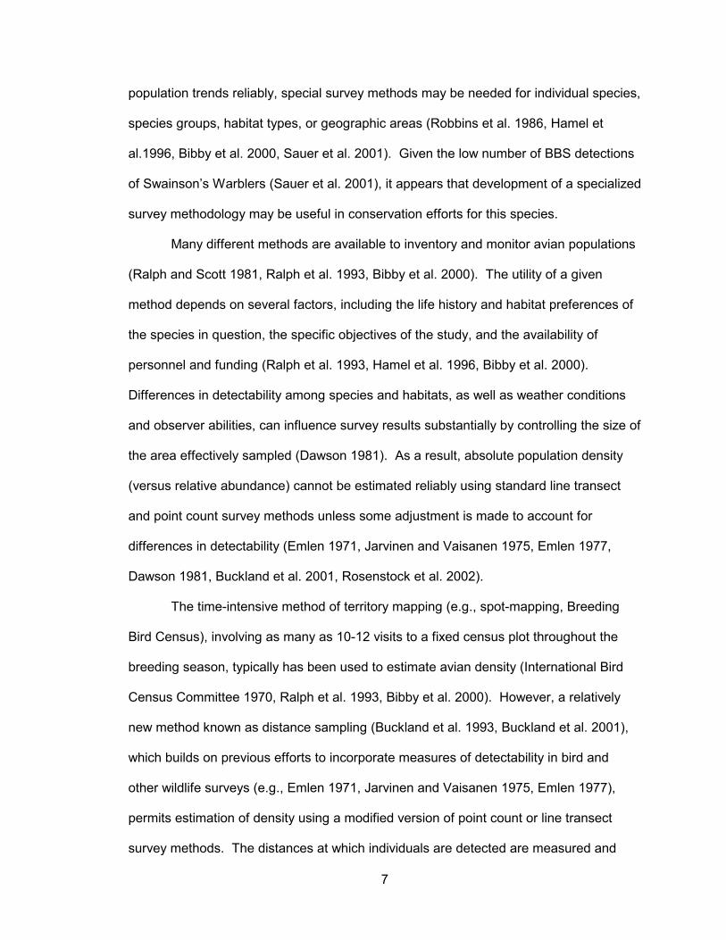
population trends reliably, special survey methods may be needed for individual species,

species groups, habitat types, or geographic areas (Robbins et al. 1986, Hamel et

al.1996, Bibby et al. 2000, Sauer et al. 2001). Given the low number of BBS detections

of Swainson’s Warblers (Sauer et al. 2001), it appears that development of a specialized

survey methodology may be useful in conservation efforts for this species.

Many different methods are available to inventory and monitor avian populations

(Ralph and Scott 1981, Ralph et al. 1993, Bibby et al. 2000). The utility of a given

method depends on several factors, including the life history and habitat preferences of

the species in question, the specific objectives of the study, and the availability of

personnel and funding (Ralph et al. 1993, Hamel et al. 1996, Bibby et al. 2000).

Differences in detectability among species and habitats, as well as weather conditions

and observer abilities, can influence survey results substantially by controlling the size of

the area effectively sampled (Dawson 1981). As a result, absolute population density

(versus relative abundance) cannot be estimated reliably using standard line transect

and point count survey methods unless some adjustment is made to account for

differences in detectability (Emlen 1971, Jarvinen and Vaisanen 1975, Emlen 1977,

Dawson 1981, Buckland et al. 2001, Rosenstock et al. 2002).

The time-intensive method of territory mapping (e.g., spot-mapping, Breeding

Bird Census), involving as many as 10-12 visits to a fixed census plot throughout the

breeding season, typically has been used to estimate avian density (International Bird

Census Committee 1970, Ralph et al. 1993, Bibby et al. 2000). However, a relatively

new method known as distance sampling (Buckland et al. 1993, Buckland et al. 2001),

which builds on previous efforts to incorporate measures of detectability in bird and

other wildlife surveys (e.g., Emlen 1971, Jarvinen and Vaisanen 1975, Emlen 1977),

permits estimation of density using a modified version of point count or line transect

survey methods. The distances at which individuals are detected are measured and

8

used to calculate a “detection function” that accounts for individuals present but not

detected in the study area; the density estimate then is adjusted accordingly (Buckland

et al. 1993, Buckland et al. 2001). Public domain software is available to carry out these

calculations (Thomas et al. 1998).

SOUTHEASTERN FLOODPLAIN FORESTS

Floodplain habitats, such as bottomland hardwood forests in the southeastern

United States, are characterized by extraordinarily high ecological productivity and

biological diversity resulting from periodic natural disturbance by flooding (Wharton et al.

1982, Keddy 2000, Brawn et al. 2001). Flood-borne sediments transport nutrients into

the terrestrial portion of the system, making soils remarkably fertile (Wharton et al.

1982, Keddy 2000, Reice 2001). Southeastern U.S. floodplains exhibit especially high

productivity as a result of climatic conditions, which provide a long growing season

(Pashley and Barrow 1993). Dynamic disturbance associated with flooding also

continually alters topography, resulting in heterogeneity of habitats – i.e., “patchiness” –

that promotes floral and faunal diversity by accommodating species with varying life

history requirements (Pashley and Barrow 1993, Brawn et al. 2001, Reice 2001).

Largely due to their high productivity, floodplain forests have been subject to

intensive human use and large-scale alteration. Bottomland hardwood forests in the

southeastern U.S. have been destroyed or degraded as the result of conversion to

agriculture and timber production, as well as alteration of natural hydrologic disturbance

regimes due to construction of flood control and water supply projects (Noss et al. 1995,

Askins 2000, Pashley et al. 2000, Sallabanks et al. 2000). It is difficult to determine the

exact amount of bottomland hardwood forest habitat lost to anthropogenic disturbance;

one estimate indicates that the 12 million ha of bottomland forest remaining today in the

9

southeastern U.S. may be less than 50% of what was present at the time of European

settlement (Hodges 1994). Others cite losses as great as 70% (Askins 2000).

Southeastern U.S. floodplains provide critical habitat for many species of birds,

as well as other wildlife (Hunter et al. 1993, Forsythe and Roelle 1990, Pashley et al.

2000, Sallabanks et al. 2000, Reice 2001). Bird species in addition to the Swainson’s

Warbler that breed in bottomland hardwood forests and have been identified as

conservation priorities include: Prothonotary Warbler (Protonaria citrea), Hooded

Warbler (Wilsonia citrina), Acadian Flycatcher (Empidonax virescens), and Yellow-Billed

Cuckoo (Coccyzus americanus). Bottomland hardwood forests also serve as important

migration corridors and stopover sites for large numbers of migratory birds that breed

elsewhere (Meanley 1971, Hunter et al. 1993, Pashley et al. 2000, Sallabanks et al.

2000). Because of their importance for both breeding and migration, and the extent to

which they have been altered and degraded by human activities, bottomland hardwood

forests are considered “habitats of special concern” for Nearctic-Neotropical migrants in

the southeastern U.S. (Hunter et al. 1993). Askins (2000) notes that a disproportionate

number of the North American bird species known or believed to be extinct were

bottomland hardwood forest specialists during the breeding and/or wintering seasons

(Carolina Parakeet, Conuropsis carolinensis; Ivory-billed Woodpecker, Campephilus

principalis; Bachman’s Warbler, Vermivora bachmanii), or used these areas intensively

during migration (Passenger Pigeon, Ectopistes migratorius).

In Georgia, it appears that private land management activities that adversely

affect bottomland forest ecosystems have increased over the past few years, following

several decades of relative stability. These include conversion of bottomlands to pine

plantations, and timber harvests involving the practice of “high-grading” in which only the

largest and most valuable trees are removed (N. Klaus, Georgia Department of Natural

Resources, personal communication). Recent drought conditions, along with human

10

population growth, may result in further degradation of floodplain forests in this region

as new dams and reservoirs are built to meet demand for water (U.S. Geological Survey

2000).

Canebrake habitats, a once-prominent feature of floodplain forests in the

southeastern U.S., may be preferred by breeding Swainson’s Warblers in some portions

of the species’s range, although localized habitat preferences appear to vary and other

shrub-level vegetation is used in areas that lack large canebrakes (Meanley 1945,

Meanley 1971, Meanley 1972, Brown and Dickson 1994, Graves 2001, Graves 2002).

These dense, nearly monotypic stands of Arundinaria gigantea, a native bamboo (family

Poaceae) commonly known as cane, covered vast areas of the southeastern U.S. at the

time of European settlement (Platt and Brantley 1997). Little is known about canebrake

ecology, in part because expansive cane stands largely were eliminated prior to the 20th

century, disappearing more quickly than any other bottomland habitat type (Platt and

Brantley 1997, Brantley and Platt 2001). Bachman’s Warbler may have been a

canebrake specialist (Remsen 1986), and many other wildlife species use canebrakes

extensively or exclusively, including the Hooded Warbler, Swamp Rabbit (Sylvilagus

aquaticus), and at least six species of Lepidoptera – five of which are listed as species

of conservation concern due to habitat alteration (Meanley 1972, Miller and Miller 1999,

Brantley and Platt 2001).

Limited research indicates that intermediate levels of disturbance – e.g., dynamic

effects of flooding and windstorms (scouring, treefalls), infrequent lighting-caused fires

that constrained growth of competing woody vegetation, and death of overstory foliage

caused by huge roosting flocks of the now-extinct Passenger Pigeon – may have

contributed historically to the development and maintenance of cane stands (Platt and

Brantley 1997, Brantley and Platt 2001). Native American agricultural practices such as

controlled burning likely expanded canebrakes (Platt and Brantley 1997, Brantley and

11

Platt 2001). However, greater anthropogenic disturbance resulting from overgrazing

and clearing of bottomlands for agriculture by European settlers, coupled with

suppression of natural disturbances such as fire and flooding, has resulted in

destruction or degradation of most canebrake communities (Platt and Brantley 1997,

Brantley and Platt 2001). It is estimated that less than 2% of the canebrakes present at

the time of European settlement remain; as a result, they are considered a “critically

endangered ecosystem” (Noss et al. 1995).

Although the “endless wilderness of canes” described by William Bartram and

others has been virtually extirpated (Platt and Brantley 1997), cane occurring as isolated

plants or small thickets remains common in many areas of the southeastern U.S. (Miller

and Miller 1999, Brantley and Platt 2001). Cane grows primarily in bottomland forest

ecosystems which are subject to seasonal flooding, yet colonies may be killed by

prolonged inundation. Large canebrakes therefore tend to occur at relatively high

elevations within the floodplain, such as the natural levee (front) immediately adjacent to

the river channel (Hodges 1994, Platt and Brantley 1997). In limited experimental

studies, fertilization promoted growth and expansion of cane (Platt and Brantley 1997),

perhaps indicating a relationship with the high soil fertility typical of floodplain forests

(Wharton et al. 1982, Keddy 2000, Platt and Brantley 2001, Reice 2001).

PREVIOUS HABITAT STUDIES

Until recently, there were few detailed quantitative studies of Swainson’s Warbler

breeding habitat preferences, although Meanley (1945, 1966, 1971) and others

published substantial descriptive information. Due to conservation concern for this

species, habitat studies since have been conducted at several sites near the edge of its

breeding range in Illinois (Eddleman et al. 1980), Missouri (Thomas et al. 1996), and

Virginia (Graves 2001), and in forests managed for commercial silviculture in South

12

Carolina (Peters 1999) and Louisiana (Bassett 2001). Results from these studies may

not reflect characteristics of breeding habitat in the species’s core breeding range

(Graves 2002), or in areas managed primarily for conservation purposes. A new study,

however, assesses habitat characteristics at five locations within the core breeding

range in Arkansas, Mississippi, Louisiana, and Florida (Graves 2002).

Swainson’s Warblers build nests in the understory (Meanley 1971, Brown and

Dickson 1994). Virtually all recent habitat studies indicate that dense shrub-layer

vegetation is critical in breeding territories, where it is typically denser than in areas

unoccupied by Swainson’s Warblers (Thomas et al. 1996, Peters 1999, Bassett 2001,

Graves 2001, Graves 2002). Overly dense understory vegetation, however, may be a

negative factor (Graves 2001). There has been conflicting evidence about the relative

importance of understory structure versus species composition (Graves 2002). The

presence of cane, once thought to be requisite in prime breeding habitat, appears to be

associated with territories in some locations, but not in others (Meanley 1971, Eddleman

et al. 1980, Thomas et al. 1996, Peters 1999, Graves 2001, Graves 2002). Specific

habitat preferences may vary geographically (Graves 2002), and according to what

shrub-level species are present.

Characteristics of ground-level habitat may be important in breeding territories

because Swainson’s Warblers forage for insects and other small arthropods almost

exclusively in leaf litter (Meanley 1971, Graves 1998). Results of previous studies

regarding leaf litter depth and coverage have been contradictory, showing no consistent

relationship between Swainson’s Warbler presence and litter layer characteristics

(Thomas et al. 1996, Peters 1999, Bassett 2001). This may be because Swainson’s

Warblers tend to nest and forage in different areas of their territories (Graves 2001), and

litter measurements thus may not have been taken in foraging areas. Graves reported

that the presence of moist organic soils covered with abundant leaf litter was

13

characteristic of territories at the Virginia site, and that litter depth and coverage may be

crucial for territories in general (Graves 1998; Graves 2001). Soil types also may

influence Swainson’s Warbler breeding distribution (Peters 1999; G. R. Graves,

Smithsonian Institution, personal communication).

Dense herbaceous ground cover may affect Swainson’s Warbler habitat use by

potentially inhibiting foraging; Meanley (1971) found little herbaceous ground cover in

breeding territories. In Louisiana and in one year of the Missouri study, areas occupied

by Swainson’s Warblers had less herbaceous ground cover than did unoccupied areas

(Thomas et al. 1996, Bassett 2001). In the Illinois study area, which had overall

herbaceous plant cover of 34%, there was virtually no herbaceous vegetation at

locations where individuals were observed foraging (Eddleman et al. 1980).

Graves (2001) identified hydrology as the “driving force” in determining the

placement of Swainson’s Warbler territories at the Virginia site: standing or pooled

water was recorded in 61% of unoccupied plots, but not in any territories. Inundation

during the breeding season may inhibit foraging, and deep flooding may destroy nests

(Meanley 1971). Hydroperiod along with flood dynamics may affect species composition

and density of vegetation (Wharton et al. 1982), as well as litter depth and coverage

(personal observation). Conversely, nutrient transport and dynamic effects of flooding

may exert positive influences on development and maintenance of appropriate

Swainson’s Warbler breeding habitat, depending on flood timing and intensity (Wharton

et al. 1982, Keddy 2000, Brawn et al. 2001). Peters (1999) recommended landscape-

scale investigations of the role of flooding and other hydrologic factors in influencing

breeding distribution of Swainson’s Warblers.

The importance of canopy height and canopy cover in Swainson’s Warbler

breeding territories is unclear. Thomas et al. (1996) found lower canopy and sub-

canopy heights in areas occupied by Swainson’s Warblers versus unoccupied areas.

14

Peters (1999) found lower canopy and midstory height at nest sites than in unoccupied

areas, but no difference in canopy height between overall territories and unoccupied

areas. Graves (in press) asserted that canopy height may not be very important in

determining suitable breeding habitat if understory requirements are met. Several

studies have found mean canopy cover (overstory trees only) of approximately 80% to

90% in areas occupied by Swainson’s Warblers, but this parameter did not differ

between occupied and unoccupied areas (Eddleman et al. 1980, Thomas et al. 1996).

Swainson’s Warblers once were thought to breed almost exclusively in late

successional forest (Meanley 1971, Graves 2002). More recently, however, breeding

populations have been discovered and studied in habitats at relatively early

successional stages, such as pine plantations and managed hardwood stands <40

years old (Carrie 1996, Peters 1999, Bassett 2001). It appears that disturbance gaps in

the forest canopy may be important in late successional habitats to promote the dense

shrub-level vegetation used for nesting (Eddleman et al. 1980, Hunter et al. 2001,

Graves 2002). There is debate over whether such gaps should be created artificially

through silvicultural practices to benefit Swainson’s Warblers, or will occur sufficiently

through natural processes (Eddleman et al. 1980, Bushman and Therres 1988, Soule et

al. 1992, Hunter et al. 2001, Graves 2002). Evidence regarding the effectiveness of

artificial gap creation in stimulating understory vegetation in bottomland forests appears

to be limited and inconclusive (Soule et al. 1992, Moorman and Guynn 2001). Whether

artificial gaps may produce adverse effects similar to those observed in conjunction with

forest fragmentation – e.g., increased nest predation or brood parasitism by Brown-

headed Cowbirds (Molothrus ater) – also is unclear and likely depends on the size of

openings created (Brawn et al. 2001, Moorman and Guynn 2001). Potential

fragmentation effects may be of special concern for Swainson’s Warblers because they

15

are considered an area-sensitive species requiring relatively large blocks of contiguous

forest habitat (Robbins et al. 1989, Kilgo et al. 1998, Graves 2002).

Two previous studies included the development of binary logistic regression

models intended to identify important characteristics of Swainson’s Warbler breeding

habitat, and to predict the presence (or absence) of breeding territories based on these

characteristics. In the Missouri study (Thomas et al. 1996), involving habitat data from

canebrakes in six different river floodplains, a three-variable model derived from 1992

data correctly classified 71% of the plots in the modeling dataset (N = 59 plots, 29

occupied and 30 unoccupied) as occupied or unoccupied by Swainson’s Warblers. This

model, however, had only 35% classification accuracy in verification with a new dataset

collected in 1993. The authors then created a five-variable model based on pooled data

for the two years (N = 90 plots, 45 occupied and 45 unoccupied), which correctly

classified 73% of the plots in the modeling data set. In this model, cane density,

overstory % canopy cover, and overstory tree diameter at breast height (dbh) were

positively correlated with Swainson’s Warbler presence, while overstory tree height and

plot distance to water were negatively correlated with Swainson’s Warbler presence. In

the Virginia study, Graves (2001) created a more successful five-variable model that

correctly classified 90% of the plots in the modeling dataset (N = 74 plots, 30 occupied

and 44 unoccupied). Smilax stem density was positively correlated with Swainson’s

Warbler presence, while cane stem density, total number of trees, number of medium-

sized trees (25-39.9 cm diameter), and basal area of swamp black gum (Nyssa sylvatica

var. biflora) were negatively correlated with Swainson’s Warbler presence. Nine more

parsimonious models created for this site, comprising two to three of the five variables

listed above, had classification accuracies of 81-87% for the modeling dataset.

Apparently, neither the Missouri habitat model based on the two-year pooled data nor

any of the Virginia models was subjected to verification or cross-validation.

16

STUDY AREA

My research was conducted at Bond Swamp National Wildlife Refuge (BSNWR;

32E44' N, 83E35' W), established in 1989 and administered by the U.S. Fish and Wildlife

Service (USFWS). BSNWR comprises 2,630 ha of forested floodplain wetlands and

adjacent uplands in Bibb and Twiggs counties, Georgia, approximately 10 km south of

Macon (Figs. 2 and 3). The refuge is managed primarily to preserve, protect, and

enhance local floodplain ecosystems associated with the Ocmulgee River, a tributary of

the Altamaha River. Most of BSNWR typically is inundated by seasonal floodwaters in

late winter through spring, although some swamp forest areas remain inundated year-

round. Specific habitat types include floodplain forest, tupelo gum (Nyssa aquatica)

swamp, and mixed pine/hardwood ridges, along with beaver swamps, oxbow lakes, and

tributary creeks (USFWS 2000).

Approximately 200 bird species are believed to use the refuge as breeding,

migration, or wintering habitat, although wildlife populations have not been well

documented. BSNWR provides habitat for one of Georgia’s three populations of black

bears (Ursus americanus), and several endangered fish species are found in this portion

of the Ocmulgee River. Non-native feral hogs pose one of the most significant threats

to the health of refuge ecosystems (USFWS 2000).

BSNWR is located in the upper portion of the Coastal Plain physiographic

province, just below the Fall Line separating the Coastal Plain from the Piedmont. In the

vicinity of the refuge, known as the Fall Line Hills District, older crystalline rocks

characteristic of the Piedmont give way to the relatively young Cretaceous sediments of

the Coastal Plain (Clark and Zisa 1976). Topography is level to rolling. The Ocmulgee

River and its tributaries in this area exhibit relatively wide floodplains and frequent

meanders (Clark and Zisa 1976).

17

Figure 2. U.S. Fish and Wildlife Service map of Bond Swamp National Wildlife Refuge,Georgia.

18

Figu

re 3

.To

pogr

aphi

c m

ap o

f Bon

d Sw

amp

Nat

iona

l Wild

life

Ref

uge

and

vici

nity

, Geo

rgia

, ada

pted

from

U.S

. Geo

logi

cal

Surv

ey M

acon

Eas

t qua

dran

gle

1:24

,000

sca

le to

pogr

aphi

c m

ap (1

981)

.

19

Climate in the vicinity is warm and humid. Mean annual high temperature at

Macon is 24 C, and mean midsummer high temperature is 32 C. Winters are relatively

short, and the growing season is long. Relative humidity averages 88% during the

morning and 54% during the afternoon. Mean annual precipitation totals 122 cm

(National Climate Data Center 2001).

Most of BSNWR is located along the east bank of the Ocmulgee River, although

USFWS recently acquired a small parcel west of the river. Only one paved road

crosses the refuge (Georgia Highway 23, near the eastern edge of the property), but

there is a network of dirt and gravel roads, as well as railroad tracks and transmission

line rights-of-way. Most roads other than the state highway have little traffic or are

abandoned. Two hiking trails cover small areas of the refuge, and hunting and fishing

are permitted seasonally in designated areas. Public use is relatively limited, however,

and a special-use permit is required for access to some areas. Few details are known

about prior land-use history. There is evidence of clear-cutting or selective timber

harvesting in most portions of the refuge, and high-grading practices may have been

employed (N. Klaus, Georgia Department of Natural Resources, personal

communication). Old-growth forest (trees >120 years old, diameter at breast height $2

m) remains in some areas (J. M. Meyers, USGS Patuxent Wildlife Research Center,

personal communication).

My study area encompassed approximately 1,740 ha of floodplain forest within

the main portion of BSNWR, bounded on the west by the Ocmulgee River and on the

east by Georgia Highway 23. This area included all bottomland hardwood forest

habitats in the main portion of the refuge, but excluded bottomlands west of the river

and pine-dominated uplands east of Highway 23. Dominant tree species in the study

area were water oak (Quercus nigra), swamp chestnut oak (Quercus michauxii), laurel

20

oak (Quercus laurifolia), overcup oak (Quercus lyrata), sweetgum (Liquidambar

styraciflua), tupelo gum (Nyssa aquatica), sugarberry (Celtis laevigata), red maple (Acer

rubrum), ash (Fraxinus sp.), American elm (Ulmus americana), and sycamore (Platanus

occidentalis), along with loblolly pine (Pinus taeda) in some areas. Approximate forest

age ranged from 30 to >120 years (J. M. Meyers, personal communication). Mean

(minimum-maximum) dbh measurements for large specimens of the dominant tree

species, based on the dbh of the largest diameter tree in each of 174 0.25-ha vegetation

plots, were 60.4 cm (36.0-121.0 cm) for water oak (n = 28 trees/plots), 64.7 cm (54.4-

94.0 cm) for swamp chestnut oak (n =10), 70.4 cm (44.8-123.6 cm) for laurel oak (n =

20), 76.8 cm (46.7-171.0 cm) for overcup oak (n = 11), 56.2 cm (38.2-74.0 cm) for

sweetgum (n = 20), 81.1 cm (52.0-125.0 cm) for tupelo gum (n = 13), 66.2 cm (46.0-

89.1 cm) for sugarberry (n = 13), 58.2 cm (44.9-86.3 cm) for red maple (n = 9), 58.6 cm

(40.2-93.2 cm) for ash species (n = 11), and 49.8 cm (40.4-60.0 cm) for loblolly pine (n

= 8) (E. A. Wright and J. M. Meyers, unpublished data).

Cane (Arundinaria gigantea) was a prominent feature of the understory,

particularly on the natural levee immediately adjacent to the river. Vines were relatively

abundant, including poison ivy (Toxicodendron radicans), greenbriar (Smilax sp.) and

grape (Vitis sp.). Sawtooth palmetto (Serenoa repens), dwarf palmetto (Sabal minor),

and semi-aquatic and aquatic forbs (e.g., Saururus cernuus, Boehmeria cylindrica,

Peltandra virginica, Sagittaria sp.) and grasses occurred in less well-drained areas,

while blackberry (Rubus sp.) dominated large sunny openings in drier areas. Invasive

exotic understory species such as Chinese privet (Ligustrum sinense), Japanese stilt

grass (Microstegium vimineum), climbing fern (Lygodium sp.) and Chinese tallow tree

(Triadica sebifera) were present in limited areas.

Meanley (1945, 1971) conducted some of his most extensive investigations of

Swainson’s Warbler natural history along the upper Ocmulgee River in the vicinity of

21

BSNWR, and described canebrakes in this area as “the ideal habitat for the breeding of

the Swainson’s Warbler.” To my knowledge, no intensive studies of Swainson’s Warbler

population status or habitat use in the Ocmulgee River floodplain have been conducted

since Meanley’s work from the 1940s through early 1970s.

RESEARCH OBJECTIVES

The specific objectives of my research were to: 1) estimate breeding population

density of Swainson’s Warblers at BSNWR; and 2) develop a habitat model that would

be sufficiently parsimonious for practical use (i.e., comprising few variables), yet highly

accurate in identifying suitable Swainson’s Warbler breeding habitat at my study site

and perhaps other locations. More generally, I sought to expand knowledge of a little

studied species in need of conservation attention, provide useful management

information, and lay the groundwork for future research.

LITERATURE CITED

American Ornithologists’ Union. 1998. The American Ornithologists’ Union check-list of

North American birds. Seventh edition. American Ornithologists’ Union,

Washington, D.C. <http://www.aou.org/aou/birdlist.html> Accessed 10

September 2001.

Anderson, S. H., and H. H. Shugart, Jr. 1974. Habitat selection of breeding birds in an

east Tennessee deciduous forest. Ecology 55:828-837.

Askins, R. A. 2000. Restoring North America’s birds: lessons from landscape ecology.

Second edition. Yale University Press, New Haven, CT.

Bassett, C. A. 2001. Habitat selection of the Swainson’s Warbler in managed forests in

southeastern Louisiana. M.S. thesis. Southeastern Louisiana University,

Hammond.

22

Bibby, C. J., N. D. Burgess, D. A. Hill, and S. Mustoe. 2000. Bird census techniques.

Second edition. Academic Press, London.

Brantley, C. G., and S. G. Platt. 2001. Canebrake conservation in the southeastern

United States. Wildlife Society Bulletin 29:1175-1181.

Brawn, J. D., S. K. Robinson, and F. R. Thompson. 2001. The role of disturbance in

ecology and conservation of birds. Annual Review of Ecology and Systematics

32:251-276.

Brown, R. E., and J. G. Dickson. 1994. Swainson’s Warbler (Limnothlypis swainsonii).

In: The birds of North America (A. Poole and F. Gill, eds.), No. 126. Academy

of Natural Sciences, Philadelphia, PA, and American Ornithologists’ Union,

Washington, D.C.

Buckland, S. T., D. R. Anderson, K. P. Burnham, and J. L. Laake. 1993. Distance

sampling: estimating abundance of biological populations. Chapman and Hall,

London.

_____, D. R. Anderson, K. P. Burnham, J. L. Laake, D. L. Borchers, and L. Thomas.

2001. Introduction to distance sampling: estimating abundance of biological

populations. Oxford University Press, New York.

Bushman, E. S., and G. D. Therres. 1988. Habitat management guidelines for forest

interior breeding birds of coastal Maryland. Maryland Department of Natural

Resources Wildlife Technical Publication 88-1. Annapolis, MD.

Bystrak, D. 1981. The North American Breeding Bird Survey. Studies in Avian Biology

6:34-41.

Carrie, N. R. 1996. Swainson’s Warblers nesting in early seral pine forests in East

Texas. Wilson Bulletin 108:802-804.

Clark, W. Z., and A. C. Zisa. 1976. Fall Line Hills District. In: Physiographic map of

Georgia. Georgia Department of Natural Resources, Atlanta, GA. < http://

23

www.cviog.uga.edu/Projects/gainfo/physiographic/FLH.htm> Accessed 16 April

2001.

Cody, M. L. 1985. An introduction to habitat selection in birds. In: Habitat selection in

birds (M. L. Cody, ed.), pp. 4-56. Academic Press, Orlando, FL.

Dawson, D. 1981. Counting birds for a relative measure (index) of density. Studies in

Avian Biology 6:12-16.

Droege, S. 1990. The North American Breeding Bird Survey. In: Survey designs and

statistical methods for the estimation of avian population trends (J. R. Sauer and

S. Droege, eds.), pp. 1-4, U.S. Fish and Wildlife Service Biological Report 90(1).

Washington, D.C.

Eddleman, W. R., K. E. Evans, and W. H. Elder. 1980. Habitat characteristics and

management of Swainson’s Warbler in southern Illinois. Wildlife Society Bulletin

8:228-233.

Emlen, J. T. 1971. Population densities of birds derived from transect counts. Auk

88:323-342.

_____. 1977. Estimating breeding season bird densities from transect counts. Auk 94:

455-468.

Finch, D. M., and P. W. Stangel. 1993. Introduction. In: Status and management of

Neotropical migratory birds (D. M. Finch and P. W. Stangel, eds.), pp. 1-4, USDA

Forest Service General Technical Report RM-229. Fort Collins, CO.

Forsythe, S. W., and J. E. Roelle. 1990. The relationship of human activities to the

wildlife function of bottom hardwood forests: the report of the wildlife workgroup.

In: Ecological processes and cumulative impacts: illustrated by bottomland

hardwood wetland ecosystems (J. L. Gosselink, L. C. Lee, and T. A. Muir, eds.),

pp. 533-546. Lewis Publishers, Chelsea, MA.

24

Fretwell, S. D., and H. L. Lucas. 1969. On territorial behavior and other factors

influencing habitat distribution in birds. Acta Biotheoretica 19:16-36.

Gill, F. B. 1995. Ornithology. Second edition. W. H. Freeman and Company, New

York.

Gough, G. A., J. R. Sauer, and M. Iliff. 1998. Patuxent bird identification infocenter.

Version 97.1. USGS Patuxent Wildlife Research Center, Laurel, MD.

<http://www.mbr-pwrc.usgs.gov/Infocenter/infocenter.html> Accessed 5

September 2001).

Graves, G. R. 1998. Stereotyped foraging behavior of the Swainson’s Warbler.

Journal of Field Ornithology 69:121-127.

_____. 2001. Factors governing the distribution of Swainson’s Warbler along a

hydrological gradient in Great Dismal Swamp. Auk 118:650-664.

_____. 2002. Habitat characteristics in the core breeding range of the Swainson’s

Warbler. Wilson Bulletin 114:210-220.

Grinnell, J. 1917. Field tests of theories concerning distributional control. American

Naturalist 51:115-128.

Hamel, P. B., W. P. Smith, D. J. Twedt, J. R. Woehr, E. Morris, R. B. Hamilton, and R.

J. Cooper. 1996. A land manager’s guide to point counts of birds in the

Southeast. USDA Forest Service General Technical Report SO-120. Asheville,

NC.

Hodges, J. D. 1994. Ecology of bottomland hardwoods. In: A workshop to resolve

conflicts in the conservation of migratory landbirds in bottomland hardwood

forests (W. P. Smith and D. N. Pashley, eds.), pp. 5-11, USDA Forest Service

General Technical Report SO-114. New Orleans, LA.

Holmes, R. T., and S. K. Robinson. 1981. Tree species preferences of foraging

insectivorous birds in a northern hardwoods forest. Oecologia 48:31-35.

25

_____, and T. S. Sherry. 2001. Thirty-year bird population change in an unfragmented

temperature deciduous forest. Auk 118:589-609.

Hunter, W. C., D. A. Buehler, R. A. Canterbury, J. L. Confer, and P. B. Hamel. 2001.

Conservation of disturbance-dependent birds in eastern North America. Wildlife

Society Bulletin 29:440-455.

_____, D. N. Pashley, and R. E. F. Escano. 1993. Neotropical migratory landbirds and

their habitats of special concern within the Southeast region. In: Status and

management of Neotropical migratory birds (D. M. Finch and P. W. Stangel,

eds.), pp. 159-171, USDA Forest Service General Technical Report RM-229.

Fort Collins, CO.

International Bird Census Committee. 1970. Recommendations for an international

standard for a mapping method for bird census work. Audubon Field Notes

24:723-726.

James, F. C. 1971. Ordinations of habitat relationships among breeding birds. Wilson

Bulletin 83:215-236.

Jarvinen, O., and R. A. Vaisanen. 1975. Estimating relative densities of breeding birds

by the line transect method. Oikos 26:316-322.

Johnson, D. H. 1980. The comparison of usage and availability measurements for

evaluating resources preference. Ecology 61:65-71.

Johnston, D. W. and E. P. Odum. 1956. Breeding bird populations in relation to plant

succession on the Piedmont of Georgia. Ecology 37:50-62.

Keddy, P. A. 2000. Wetland ecology: principles and conservation. Cambridge

University Press, Cambridge, UK.

Keller, C. M. E., and J. T. Scallan. 1999. Potential roadside biases due to habitat

changes along Breeding Bird Survey routes. Condor 101:50-57.

26

Kilgo, J. C., R. A. Sargent, B. R. Chapman, and K. V. Miller. 1998. Effect of stand width

and adjacent habitat on breeding bird communities in bottomland hardwoods.

Journal of Wildlife Management 62:72-83.

Lack, D. 1933. Habitat selection in birds, with special reference to the effects of

afforestation on the Breckland avifauna. Journal of Animal Ecology 2:239-262.

Lovejoy, T. E. 1992. Foreword. In: Ecology and conservation of neotropical migrant

landbirds (J. M. Hagan III and D. W. Johnston, eds.), pp. ix-x. Smithsonian

Institution Press, Washington, D.C.

MacArthur, R. H., and J. W. MacArthur. 1961. On bird species diversity. Ecology

42:594-598.

Marra, P. P., K. A. Hobson, and R.T. Holmes. 1998. Linking winter and summer events

in a migratory bird using stable carbon isotopes. Science 282:1884-1886.

Martin, T. E. 1992. Breeding productivity considerations: what are the appropriate

habitat features for management? In: Ecology and conservation of neotropical

migrant landbirds (J. M. Hagan III and D. W. Johnston, eds.), pp. 455-473.

Smithsonian Institution Press, Washington, D.C.

_____. 1998. Are microhabitat preferences of coexisting species under selection and

adaptive? Ecology 79:656-670.

Meanley, B. 1945. Notes on Swainson’s Warbler in central Georgia. Auk 62:395-401.

_____. 1966. Some observations on habitats of the Swainson’s Warbler. Living Bird

5:151-165.

_____. 1971. Natural history of the Swainson’s Warbler. U.S. Department of the

Interior, Bureau of Sport Fisheries and Wildlife, North American Fauna No. 69.

Washington, D.C.

_____. 1972. Swamps, river bottoms, and canebrakes. Barre Publishers, Barre, MA.

27

Miller, J. H., and K. V. Miller. 1999. Forest plants of the Southeast and their wildlife

uses. Southern Weed Science Society, Champaign, IL.

Moorman, C. E., and D. C. Guynn, Jr. 2001. Effects of group-selection opening size on

breeding bird habitat use in a bottomland forest. Ecological Applications

11:1680-1691.

National Climate Data Center. 2001. National Climate Data Center online search

engine. U.S. Department of Commerce, National Oceanic and Atmospheric

Administration, Washington, D.C. <http://www.ncdc.noaa.gov/ol/climate/

climateresources.html> Accessed 15 April 2001.

Noss, R. F., E. T. LaRoe III, and J. M. Scott. 1995. Endangered ecosystems of the

United States: a preliminary assessment of loss and degradation. U.S.

Department of the Interior, National Biological Survey, Biological Report 28.

Washington, D.C. <http://biology.usgs.gov/pubs/ecosys.htm> Accessed 4

September 2001.

Pashley, D. N., and W. C. Barrow. 1993. Effects of land use practices on Neotropical

migratory birds in bottomland hardwood forests. In: Status and management of

Neotropical migratory birds (D. M. Finch and P. W. Stangel, eds.), pp. 315-320,

USDA Forest Service General Technical Report RM-229. Fort Collins, CO.

_____, C. J. Beardmore, J. A. Fitzgerald, R. P. Ford, W. C. Hunter, M. S. Morrison, and

K. V. Rosenberg. 2000. Partners in Flight: conservation of the land birds of the

United States. American Bird Conservancy, The Plains, VA.

Peterjohn, B. G., J. R. Sauer, and C. S. Robbins. 1995. Population trends from the

North American Breeding Bird Survey. In: Ecology and management of

Neotropical migratory birds: a synthesis and review of critical issues (T. E. Martin

and D. M. Finch, eds.), pp. 3-35. Oxford University Press, New York.

28

Peters, K. A. 1999. Swainson’s Warbler (Limnothlypis swainsonii) habitat selection in a

managed bottomland hardwood forest in South Carolina. M.S. thesis. North

Carolina State University, Raleigh.

Platt, S. G., and C. G. Brantley. 1997. Canebrakes: an ecological and historical

perspective. Castanea 62:8-21.

Ralph, C. J., G. R. Geupel, P. Pyle, T. E. Martin, and D. F. DeSante. 1993. Handbook

of field methods for monitoring landbirds. USDA Forest Service General

Technical Report PSW-GTR-144. Albany, CA.

_____, and J. M. Scott, eds. 1981. Estimating numbers of terrestrial birds. Studies in

Avian Biology No. 6.

Rappole, J. H., E. S. Morton, T. E. Lovejoy III, and J. L. Ruos. 1995. Nearctic avian

migrants in the Neotropics. Second edition. Smithsonian Institution,

Conservation and Research Center, Front Royal, VA.

Reice, S. R. 2001. The silver lining: the benefits of natural disasters. Princeton

University Press, Princeton, NJ.

Robbins, C. S., D. Bystrak, and P. H. Geissler. 1986. The Breeding Bird Survey: its

first fifteen years, 1965-1979. U.S. Fish and Wildlife Service Resource

Publication 157. Washington, D.C.

_____, D. K. Dawson, and B. A. Dowell. 1989. Habitat area requirements of breeding

forest birds of the Middle Atlantic states. Wildlife Monographs 103:1-34.

_____, C. S., J. R. Sauer, and B. G. Peterjohn. 1993. Population trends and

management opportunities for neotropical migrants. In: Status and


eds.), pp. 17-23, USDA Forest Service General Technical Report RM-229. Fort

Collins, CO.

29

Robinson, S. K., and R. T. Holmes. 1984. Effects of plant species and foliage structure

on the foraging behavior of forest birds. Auk 101:672-684.

Roosevelt, T. 1908. In the Louisiana canebrakes. Scribner’s Magazine 43:47-60.

<http://pantheon.cis.yale.edu/~thomast/texts/cane/cane.html> Accessed 8 April

2001.

Rosenstock, S. S., D. R. Anderson, K. M. Giesen, T. Leukering, and M. F. Carter. 2002.

Landbird counting techniques: current practices and an alternative. Auk 119:46-

53.

Rotenberry, J. T. 1985. The role of habitat in avian community composition:

physiognomy or floristics? Oecologia 67:213-217.

Sallabanks, R., J. R. Walters, and J. A. Collazo. 2000. Breeding bird abundance in

bottomland hardwood forests: habitat, edge, and patch size effects. Condor

102:748-758.

Sauer, J. R., J. E. Hines, and J. Fallon. 2001. The North American Breeding Bird

Survey: results and analysis 1966-2000. Version 2001.2. USGS Patuxent

Wildlife Research Center, Laurel, MD. <http://www.mbr-pwrc.usgs.gov/bbs/

bbs.html> Accessed 22 September 2001.

Sherry, T. W. and R. T. Holmes. 1995. Summer versus winter limitation of populations:

what are the issues and what is the evidence? In: Ecology and management of



Soule, J., G. Hammerson, and D. W. Mehlman. 1992. Swainson’s Warbler

(Limnothlypis swainsonii). In: Wings info resources: species information and

management abstracts. The Nature Conservancy, Arlington, VA. <http://

www.tnc.org/wings/wingsresources/swwa.html> Accessed 5 September 2001.

30

Terborgh, J. 1989. Where have all the birds gone? Princeton University Press,

Princeton, NJ.

Thomas, B. G., E. P. Wiggers, and R. L. Clawson. 1996. Habitat selection and

breeding status of Swainson’s Warblers in southern Missouri. Journal of Wildlife

Management 60:611-616.

Thomas, L., J. L. Laake, J. F. Derry, S. T., Buckland, D. L. Borchers, D. R. Anderson, K.

P. Burnham, S. Strindberg, S. L. Hedley, M. L. Burt, F. Marques, J. H. Pollard,

and R. M. Fewster. 1998. Distance 3.5, release 6 (software). Research Unit for

Wildlife Population Assessment, University of St. Andrews, St. Andrews, UK.

<http://www.ruwpa.st-and.ac.uk/distance/> Accessed 22 September 2002.

U.S. Fish and Wildlife Service. 2000. Bond Swamp National Wildlife Refuge

(brochure). U.S. Fish and Wildlife Service, Washington, D.C.

U.S. Geological Survey. 2000. USGS fact sheet: Georgia. FS-011-99. U.S.

Geological Survey, Reston, VA. <http://water.usgs.gov/pubs/FS/FS-011-99>

Accessed 10 April 2001.

Wharton, C. H., W. M. Kitchens, and T. W. Sipe. 1982. The ecology of bottomland

hardwood swamps of the Southeast: a community profile. U.S. Fish and Wildlife

Service, Biological Services Program, FWS/OBS-81/37. Washington, D.C.

Chapter 2

ESTIMATING DENSITY OF A SWAINSON’S WARBLER

BREEDING POPULATION WITH DISTANCE SAMPLING1

1Wright, E. A. and J. M. Meyers. To be submitted to Journal of Field Ornithology.

32

ABSTRACT

We used distance sampling methods to estimate breeding population density of

Swainson’s Warblers (Limnothlypis swainsonii), an inadequately monitored Nearctic-

Neotropical migrant songbird species of high conservation concern, in 2001 at a 1,740-

ha floodplain forest site within Bond Swamp National Wildlife Refuge, Georgia. We

detected 27 Swainson’s Warblers along 21 random transects with total length of 18.36

km. Mean density of Swainson’s Warbler breeding territories (singing males) in our

study area was 9.4/km2, and mean abundance was 163 singing males. Our distance

sampling results had high variances (CV = 0.298) due primarily to low encounter rate,

but appear reasonable based on our knowledge of the population at this site derived

from mapping of Swainson’s Warbler locations, tape playback surveys, and other

methods we used in 2 yr of a related habitat study. Distance sampling may not be very

effective for monitoring Swainson’s Warbler populations in general, because we were

unable to obtain density and abundance estimates with low variances even at a site with

a relatively large population at apparently high density. Further research is needed to

determine the best methods for assessing population status and trends in rare to

uncommon species such as the Swainson’s Warbler.

Key words: Swainson’s Warbler, Limnothlypis swainsonii, distance sampling, Bond

Swamp, breeding population density, Nearctic-Neotropical migrant, bird survey

methods.

33

INTRODUCTION

Existing broad-scale avian monitoring programs such as the annual Breeding

Bird Survey (BBS), which uses road-based sampling, do not sample all species,

habitats, and geographic regions equally well (Bystrak 1981, Sauer et al. 2001). BBS

methods may not adequately sample species that are uncommon or elusive, that have

restricted breeding ranges or patchy (uneven) distributions, or that breed in habitats not

well represented along roads (e.g., forest interior species, wetland species) (Bystrak

1981, Robbins et al. 1986, Keller and Scallan 1999). Riparian species may be

undersampled on BBS routes in the eastern lowlands, due to the typical orientation of

roads with respect to floodplain topography (Droege 1990).

The Swainson’s Warbler (Limnothlypis swainsonii), a cryptically colored and

relatively uncommon Nearctic-Neotropical migratory songbird that breeds predominantly

in floodplain forests of the southeastern United States (Brown and Dickson 1994), is an

example of a species inadequately monitored by BBS methods. Relative abundance of

Swainson’s Warblers on BBS routes within the species’s breeding range (Eastern and

Central BBS regions) for 1966-2000 was only 0.12-0.13 individuals per route. Analysis

of BBS data shows no significant trend (at α = 0.05) in Swainson’s Warbler populations

survey-wide during this period (trend +2.9%; p = 0.07; N = 108 routes; 95% confidence

interval = -0.2-6.0%; relative abundance = 0.12 individuals/ route). Due to the species’s

low relative abundance, BBS results are so imprecise that a long-term population

change of 3-5% per year would be undetectable (Sauer et al. 2001).

Anecdotal evidence suggests that Swainson’s Warbler populations may be

declining as the result of agricultural, forestry, and watershed management practices

that have altered floodplains in the southeastern U.S. substantially (Brown and Dickson

1994, Askins 2000, Pashley et al. 2000). The Swainson’s Warbler is considered an

extremely high priority species for conservation attention under the Partners in Flight

34

species prioritization scheme (Pashley et al. 2000). Additional information about this

species’s population status and trends is required for conservation and management

(Brown and Dickson 1994, Hamel et al. 1996, Pashley et al. 2000).

Line transect or point count surveys provide only an index to relative abundance

– not an estimate of absolute density – unless variation in detectability occurring among

species and habitats, or resulting from factors such as weather conditions and observer

abilities, is taken into account (Emlen 1971, Jarvinen and Vaisenen 1975, Emlen 1977,

Buckland et al. 1993, Bibby et al. 2000, Buckland et al. 2001). The time-intensive

method of territory mapping (e.g., spot-mapping, Breeding Bird Census), which involves

multiple visits to a fixed census plot throughout the breeding season, traditionally has

been used to estimate avian density (International Bird Census Committee 1970, Bibby

et al. 2000). However, a newer set of methods collectively known as distance sampling

(Buckland et al. 1993, Buckland et al. 2001) permits estimation of density using modified

point count or line transect survey techniques. The observer measures and records the

distance from the point or transect to each individual bird detected. These distance data

are used to derive a “detection function” that accounts for individuals present but not

detected in the study area, and the density estimate is adjusted accordingly (Buckland

et al. 1993, Buckland et al. 2001).

We used distance sampling methods to estimate density of Swainson’s Warbler

breeding territories within a floodplain forest located in central Georgia, U.S. To our

knowledge, such methods have not been used previously for this species nor have they

been used extensively for bird surveys in similar habitats. Other methods we used to

locate and map Swainson’s Warbler territories as part of a related habitat study provided

information to assess the efficiency and effectiveness of our distance sampling survey.

35

STUDY AREA

We conducted our study within Bond Swamp National Wildlife Refuge (BSNWR;


Service (USFWS). BSNWR comprises 2,630 ha of forested wetlands and adjacent

uplands in Bibb and Twiggs counties, Georgia, approximately 10 km south of Macon.

The refuge is managed primarily to preserve, protect, and enhance local floodplain

ecosystems associated with the Ocmulgee River, a tributary of the Altamaha River.

Most of the refuge typically is inundated by seasonal floodwaters in late winter through

early spring, although some portions remain inundated year-round. Habitat types

include bottomland hardwood forest, tupelo gum (Nyssa aquatica) swamp, and mixed

pine/hardwood ridges, along with beaver swamps, oxbow lakes, and tributary creeks

(USFWS 2000). Topography is level to rolling; the Ocmulgee River and its tributaries in

this area exhibit relatively wide floodplains and frequent meanders (Clark and Zisa

1976). Climate is warm and humid. Mean annual high temperature at Macon is 24 C,

and mean midsummer high temperature is 32 C. Relative humidity averages 88%

during the morning and 54% during the afternoon, and mean annual precipitation totals

122 cm (National Climate Data Center 2001).

Our study area encompassed approximately 1,740 ha of bottomland hardwood

forest bounded on the west by the Ocmulgee River and on the east by Georgia Highway

23, thus encompassing nearly all floodplain forest habitats within the refuge. Dominant

tree species were water oak (Quercus nigra), swamp chestnut oak (Quercus michauxii),

laurel oak (Quercus laurifolia), overcup oak (Quercus lyrata), sweetgum (Liquidambar


rubrum), ash (Fraxinus sp.), American elm (Ulmus americana), sycamore (Platanus

occidentalist), and loblolly pine (Pinus taeda). Forest age ranged from approximately 30

to >120 years. Cane (Arundinaria gigantea) was a prominent feature of the understory,

36

particularly on the natural levee adjacent to the river; in other areas, sawtooth palmetto

(Serenoa repens), dwarf palmetto (Sabal minor), blackberry (Rubus sp.), or aquatic and

semi-aquatic forbs and grasses dominated the understory.

METHODS

We conducted surveys for Swainson’s Warblers along 21 transects of unequal

lengths, totaling 18.36 km, between 31 May and 20 June 2001 (non-continuous; surveys

were suspended for approximately 1 wk due to flooding that prevented site access).

Groups of transects were established systematically from random starting points in each

portion of the study area, oriented to cross anticipated ecological gradients. The

starting point for the first transect in each group was placed at a randomly selected

distance of 175-200 m from the refuge boundary. Subsequent transects in the same

area were parallel to the first transect, and were separated from adjacent transects by

randomly selected distances of 350-400 m. The 21 transects thus covered most

bottomland and wetland areas within the refuge to ± 200 m on each side of the transect.

We marked the entire length of each transect with biodegradable cotton twine, recorded

its compass bearing, and obtained Universal Transverse Mercator (UTM; NAD 83)

coordinates for its start and end points using a Magellan XL2000 hand-held Global

Positioning System (GPS) unit.

Each transect was surveyed by a single observer who walked its length starting

at local sunrise and ending within 2 h. Upon detecting a Swainson’s Warbler, we used a

compass bearing relative to the transect bearing to move to a point on the transect

perpendicular to the bird’s location. We recorded UTM coordinates for that point, and

measured the perpendicular distance (m) from the point to the bird. Laser rangefinders

were used for distance measurements where possible, but understory vegetation was

typically too dense. Most distances were measured by pacing to the bird’s location;

37

paces subsequently were converted to meters based on each observer’s measured

pace length.

We used Distance 3.5 software (Thomas et al. 1998) to estimate density and

abundance of singing (territorial) males at BSNWR from the transect survey data,

following methods outlined in Buckland et al. (2001). We employed visual examination

of histograms and chi-square goodness-of-fit tests as complementary techniques to

determine whether our transect survey data should be grouped into distance intervals

prior to modeling. Based on this exploratory analysis, we grouped our data into 30-m

intervals (Fig. 4) to improve their fit to a generalized detection function curve, and to

reduce the effect of minor measurement errors that may have occurred during data

collection (Buckland et al. 2001). We ran six types of analytical models (varying

combinations of key functions and series expansions) recommended by Buckland et al.

(2001) as robust for analysis of line transect survey data: uniform + cosine, uniform +

simple polynomial, half-normal + cosine, half-normal + hermite polynomial, hazard-rate

+ cosine, and hazard-rate + simple polynomial. Akaike’s Information Criterion (AIC)

scores were used to select the best model (lowest AIC) for density estimation.

We also located Swainson’s Warbler territories at BSNWR by four other

methods during the 2001 breeding season, as part of a related habitat study: intensive

searches, opportunistic detections during site reconnaissance and transect layout, tape

playback surveys, and single-visit territory mapping. For individuals located by the first

two methods, we recorded UTM coordinates of the location from which the observer first

detected the bird, the distance (meters) and compass bearing from that point to the bird,

and the detection method (aural or visual).

Tape playback surveys were conducted along the same transects used for the

distance sampling surveys, on the same morning and immediately following completion

of each distance sampling survey. We played pre-recorded Swainson’s Warbler songs

38

0

2

4

6

8

10

12

30 60 90 120

Figure 4. Swainson’s Warbler detections in transect surveys at Bond SwampNational Wildlife Refuge, Georgia, 31 May-20 June 2001; detection distancesgrouped into 30-m intervals (cutpoint is interval upper bound).

Num

ber o

f ind

ivid

uals

det

ecte

d

Distance interval cutpoint (m)

39

and calls every 250-300 m while walking back from the transect’s end point to its start

point. At each playback location, we broadcast 2-3 song phrases followed by chip notes

for 20-30 s on portable cassette recorders with amplified 5-cm speakers (Radio Shack

model AMX9, output 2 w) set to a volume approximating normal vocalizations. We

recorded the UTM coordinates of each playback location, the approximate distance and

compass bearing from that location to each Swainson’s Warbler detected within 3 min

after the tape broadcast, and the detection method. We did not derive a density

estimate from the playback data because exploratory modeling efforts indicated that

movement toward the observer would have altered the detection function and produced

an unrealistically high density estimate, as suggested by Buckland et al. (1993).

However, we used Distance 3.5 to determine encounter rate and effective strip width

surveyed with playback.

Territory mapping occurred from early May through mid-June. We followed

singing males as they moved through their territories, maintaining a distance of at least

10 m between the observer and the bird, and used GPS units to record UTM

coordinates for each location at which the individual bird was observed. Each individual

was followed for at least 1-2 h, or for a longer period if necessary to obtain a minimum

of 10 locations. Most territories were mapped in a single visit, but we made repeated

visits over several days or weeks in a few instances to obtain a sufficient number of

locations. We produced a map of each territory using Microsoft Excel 97 software

(Microsoft Corporation 1996) to create a scatterplot of the UTM East and North

coordinates for each location at which the individual was observed.

RESULTS

We detected 27 Swainson’s Warblers, all of which were singing males, in our

distance sampling transect surveys. The encounter rate (rate at which individuals were

40

detected per unit transect length) was 1.47 singing males/km (CV = 0.238; df = 20).

The greatest distance at which an individual was detected was 120 m. Probability of

detection for an individual within the area bounded by this maximum detection distance

was 0.65 (CV = 0.179; df = 26), and effective strip width surveyed on each side of

transects (maximum detection distance x probability of detection) was 78.5 m (CV =

0.179; df = 26). Two models had identical AIC scores that were the lowest among all

our models: half-normal + cosine and half-normal + hermite polynomial (both with AIC =

72.601). These models produced identical density estimates of 9.4 singing males

(territories)/km2 (95% confidence interval = 5.2-16.9 singing males (territories)/km2; CV

= 0.298; df = 39). Estimated number of Swainson’s Warbler territories (i.e., abundance

of singing males) in our study area was 163 (95% confidence interval = 90-294; CV =

0.298; df = 39).

In tape playback surveys, we detected 43 Swainson’s Warblers within the study

area boundaries, 10 of which responded only with chip notes; we thus could not

determine whether these 10 individuals were territorial males. Overall encounter rate

(singing males plus chipping birds of unknown sex) in the playback surveys was 2.3

individuals/km (CV = 0.18; df = 20). Effective strip width surveyed was 30.9 m (CV =

0.117; df = 41).

We mapped 56 individual Swainson’s Warbler territories using a mean of 19.2

locations (SE = 0.91) per territory. The total number of individuals we detected through

intensive searches and opportunistic detections (excluding detections we determined

were duplicate observations of a previously detected individual) was 86, of which 84

were singing males.

41

DISCUSSION

The number of Swainson’s Warblers detected in our transect surveys was below

the minimum standards for density estimation using distance sampling methods.

Buckland et al. (1993, 2001) recommend at least 60-80 observations, although as few

as 40 may suffice in some cases. A study evaluating the effectiveness of distance

sampling using older analysis methods (software program TRANSECT) suggested that

at least 100 observations may be required to produce a reliable density estimate (Verner

and Ritter 1988). Still, our mean density and abundance estimates appear reasonable

given our knowledge of Swainson’s Warbler populations at BSNWR derived from tape

playback surveys, territory mapping, and other methods. During the 2002 breeding

season, 54 singing males were detected and 36 territories mapped in portions of the

study area where we had been unable to conduct intensive searches or map territories

in 2001; we also re-located many of the 2001 territories, but did not re-map them, in

2002 (J. M. Meyers, unpublished data). Our combined data for 2001 and 2002

represent coverage of 100% of the study area over the 2 yr. While we cannot be certain

that each 2002 detection represented an additional territory not counted in 2001, or that

our counts of singing males did not include duplicate detections (since not all territories

were mapped), the overall number of singing males detected during the 2 yr (138) was

relatively close to our mean abundance estimate (163) from distance sampling.

Meanley (1971) reported an encounter rate of 5.9 singing males/km on a 3.2-km

transect in the Bond Swamp area in 1968, but this may represent maximal (versus

mean) abundance or may include migrants (no date specified). During migration (3 May

2001), Meyers encountered 6.0 males/km on a 2.5-km transect (oriented North-South)

in optimal habitat along the Ocmulgee River at BSNWR (J. M. Meyers, unpublished

data). Graves (in press) reported approximate densities at five sites in four states within

the species’s core breeding range (Arkansas, Florida, Louisiana, Mississippi) derived

42

from transect surveys involving at least 3 independent continuous playback runs for

each transect (playback along entire transect; runs on different days) (G. R. Graves,

personal communication). Extrapolating from his results, mean density for these five

sites was approximately 10 males/km2 (range = 3.8-20.5 males/km2) – similar to the

mean density estimate for our study area derived through distance sampling. Prior

estimates of Swainson’s Warbler abundance and density may not be directly

comparable to our results, however, due to variation in survey methods, scales, and

timing, as well as the quality of habitat surveyed (Brown and Dickson 1994).

The small number of detections in our distance sampling surveys, relative to the

number of territories and individuals we determined were present by other methods in

2001, may have resulted in part from survey timing. Individuals were not singing as

intensively during our transect surveys as they had been 2-4 wk earlier (~30% reduction

in singing rates), and the delay in our surveys due to flooding may have exacerbated

this problem. Singing behavior may change as the breeding season progresses, and

earlier surveys – perhaps commencing in mid-May (~15-21 May in our study area) –

may be warranted for Swainson’s Warblers (Wilson and Bart 1985; Meanley 1968,

1971; Brown and Dickson 1994; G. R. Graves, personal communication). However,

surveys conducted too early may be problematic due to the presence of migrating

individuals that may not remain to breed in the area surveyed.

Distance sampling methods may be ineffective for detecting changes in

populations of relatively rare species such as the Swainson’s Warbler. We were unable

to achieve the recommended number of detections although we surveyed a relatively

large area with a substantial population at apparently high density. Nearly two-thirds of

the variance associated with our density estimate (63.8%) was attributable to encounter

rate – i.e., the relatively small number of individuals we detected. Where Swainson’s

43

Warblers are less abundant or breed at lower densities, it may be impossible to obtain

density estimates with low variances through distance sampling.

Further research is needed regarding the relative effectiveness of distance

sampling and alternate density estimation methods for Swainson’s Warblers and other

uncommon species in habitats not adequately sampled by BBS methods. To gauge

population trends reliably, special survey methods may be needed for individual species,

species groups, or habitat types (Robbins et al. 1986, Hamel et al.1996, Bibby et al.

2000, Sauer et al. 2001).

Although we employed it primarily to locate habitat plots, our single-visit mapping

approach appeared to be efficient in delineating territories at BSNWR. We spent ~2-3

person-hours locating and mapping the movements of each individual, and are confident

that the 56 areas we mapped represent discrete territories based on counter-singing we

heard and visual examination of our maps. (We eliminated from our dataset several

additional territories that we believed might be duplicates.) In comparison, we

expended ~4.5 person-hours for each detection obtained in our distance sampling

transect surveys, about 50% to conduct the surveys and 50% for transect layout.

More than one visit (i.e., mapping on >1 day) may be needed to map Swainson’s

Warbler territories adequately. However, the standard breeding bird spot-mapping

approach, involving as many as 10-12 visits to each territory spaced throughout the

breeding season, may be infeasible both because of its labor-intensiveness and

because shifts in territory occupancy may occur with re-nesting or double-brooding (J. L.

Thompson, North Carolina State University, personal communication). Bibby et al.

(2000) suggest that as few as five appropriately timed visits may suffice for single-

species territory mapping. A mapping approach involving five or fewer visits in mid-May

to mid-June (Meanley 1971, Peters 1999) may be adequate to estimate population

density. It also could facilitate collection of additional habitat data and reproductive data

44

– e.g., through identification of nest locations for intensive monitoring and/or observation

of reproductive index parameters (Vickery et al. 1992) – needed to assess demography

and long-term viability of Swainson’s Warbler populations (VanHorne 1983, Pulliam

1988, Martin 1992, Brown and Dickson 1994).

Tape playback may be useful in locating individuals and mapping territories,

based on our work and that of Graves (1996, in press). This approach, however, should

be used with caution given the potential for movement of individuals toward the observer

– as evidenced by the 61% reduction in effective strip width in our playback surveys,

compared with unaided surveys – and possibly far outside their normal territory

boundaries (R. J. Cooper, University of Georgia, personal communication). Potential

adverse effects of investigator disturbance on breeding populations also should be

considered when using tape playback (Brown and Dickson 1994).

Meyers and Odum (2000) emphasize the inherent difficulty of monitoring

uncommon to rare bird species. As our study shows, it may be difficult or impossible to

obtain reliable density and abundance estimates for use in determining Swainson’s

Warbler population trends through distance sampling. Both distance sampling and

territory mapping methods of density estimation may be too labor-intensive for

widespread practical use. It may be appropriate to monitor Swainson’s Warbler

breeding populations by collecting presence/absence data over a large geographic area,

perhaps employing tape playback, and using a probability approach based on changes

in occurrence over time to assess population trends (Nichols et al. 1998a, Nichols et al.

1998b, Meyers and Odum 2000).

ACKNOWLEDGMENTS

Financial and in-kind support for this research was provided by The University of

Georgia’s Warnell School of Forest Resources, Alumni Foundation Scholarship; U.S.

45

Fish and Wildlife Service; USGS Patuxent Wildlife Research Center; and Georgia

Ornithological Society, H. Branch Howe, Jr. Graduate Student Research Grant.

Piedmont National Wildlife Refuge personnel, especially C. Johnson and R. Shell,

offered extensive logistical support. K. Owens and J. Strong assisted with fieldwork

under often difficult conditions. We also thank C. Moore and R. Cooper for statistical

advice, B. Fancher for assistance with data management and project paperwork, and C.

and R. Leavell and their staff for excellent field housing at Charlane Plantation.

LITERATURE CITED





Hammond.

Bibby, C. J., N. D. Burgess, D. A. Hill, and S. Mustoe. 2000. Bird census techniques.

Second edition. Academic Press, London.




Washington, D.C.

Buckland, S. T., D. R. Anderson, K. P. Burnham, and J. L. Laake. 1993. Distance

sampling: estimating abundance of biological populations. Chapman and Hall,

London.

_____, D. R. Anderson, K. P. Burnham, J. L. Laake, D. L. Borchers, and L. Thomas.

2001. Introduction to distance sampling: estimating abundance of biological

populations. Oxford University Press, New York.

46

Bystrak, D. 1981. The North American Breeding Bird Survey. Studies in Avian Biology

6:34-41.


Georgia. Georgia Department of Natural Resources, Atlanta, GA. <http://

www.cviog.uga.edu/Projects/gainfo/physiographic/FLH.htm> Accessed 16 April

2001.

DeSante, D. 1992. Monitoring Avian Productivity and Survivorship (MAPS): a sharp,

rather than blunt, tool for monitoring and assessing landbird populations. In:

Wildlife 2001: populations (D. R. McCullough and R. H. Barrett, eds.), pp. 511-

521. Elsevier Applied Science, London.

Droege, S. 1990. The North American Breeding Bird Survey. In: Survey designs and

statistical methods for the estimation of avian population trends (J. R. Sauer and

S. Droege, eds.), pp. 1-4, U.S. Fish and Wildlife Service Biological Report 90(1).

Washington, D.C.

Emlen, J. T. 1971. Population densities of birds derived from transect counts. Auk

88:323-342.

_____. 1977. Estimating breeding season bird densities from transect counts. Auk 94:

455-468.

Graves, G. R. 1996. Censusing wintering populations of Swainson’s Warblers in the

Blue Mountains of Jamaica. Wilson Bulletin 108:94-103.



Hamel, P. B., W. P. Smith, D. J. Twedt, J. R. Woehr, E. Morris, R. B. Hamilton, and R.

J. Cooper. 1996. A land manager’s guide to point counts of birds in the

Southeast. USDA Forest Service General Technical Report SO-120. Asheville,

NC.

47

International Bird Census Committee. 1970. Recommendations for an international

standard for a mapping method for bird census work. Audubon Field Notes

24:723-726.

Jarvinen, O., and R. A. Vaisanen. 1975. Estimating relative densities of breeding birds

by the line transect method. Oikos 26:316-322.

Keller, C. M. E., and J. T. Scallan. 1999. Potential roadside biases due to habitat

changes along Breeding Bird Survey routes. Condor 101:50-57.





Meanley, B. 1968. Singing behavior of the Swainson’s Warbler. Wilson Bulletin 80:72-

77.



Washington, D.C.

Meyers, J. M., and E. P. Odum. 2000. Early avian research at the Savannah River Site:

historical highlights and possibilities for the future. Studies in Avian Biology 21:

18-31.





Nichols, J. D., T. Boulinier, J. E. Hines, K. H. Pollock, and J. R. Sauer. 1998a.

Estimating rates of local species extinction, colonization, and turnover in animal

communities. Ecological Applications 8:1213-1225.

48

Nichols, J. D., T. Boulinier, J. E. Hines, K. H. Pollock, and J. R. Sauer. 1998b.

Inference methods for spatial variation in species richness and community

composition when not all species are detected. Conservation Biology 12:1390-

1398.

Pashley, D. N., C. J. Beardmore, J. A. Fitzgerald, R. P. Ford, W. C. Hunter, M. S.

Morrison, and K. V. Rosenberg. 2000. Partners in Flight: conservation of the

land birds of the United States. American Bird Conservancy, The Plains, VA.




Pulliam, H. R. 1988. Sources, sinks, and population regulation. American Naturalist

132:652-661.

Ralph, C. J., G. R. Geupel, P. Pyle, T. E. Martin, and D. F. DeSante. 1993. Handbook

of field methods for monitoring landbirds. USDA Forest Service General

Technical Report PSW-GTR-144. Albany, CA.

Revels, M. 2001. The Swainson’s Warbler: a summer of looking, listening, and

learning. Sutton Newsletter (G. M. Sutton Avian Research Center) 17:4-5.

Robbins, C. S., D. Bystrak, and P. H. Geissler. 1986. The Breeding Bird Survey: its

first fifteen years, 1965-1979. U.S. Fish and Wildlife Service Resource

Publication 157. Washington, D.C.

Sauer, J. R., J. E. Hines, and J. Fallon. 2001. The North American Breeding Bird

Survey: results and analysis 1966-2000. Version 2001.2. USGS Patuxent

Wildlife Research Center, Laurel, MD. <http://www.mbr-pwrc.usgs.gov/bbs/

bbs.html> Accessed 22 September 2002.

Thomas, L., J. L. Laake, J. F. Derry, S. T., Buckland, D. L. Borchers, D. R. Anderson, K.

P. Burnham, S. Strindberg, S. L. Hedley, M. L. Burt, F. Marques, J. H. Pollard,

49

and R. M. Fewster. 1998. Distance 3.5, release 6 (software). Research Unit for

Wildlife Population Assessment, University of St. Andrews, St. Andrews, UK.

<http://www.ruwpa.st-and.ac.uk/distance/> Accessed 22 September 2002.



VanHorne, B. 1983. Density as a misleading indicator of habitat quality. Journal of

Wildlife Management 47:893-901.

Verner, J., and L. V. Ritter. 1988. A comparison of transects and spot-mapping in oak-

pine woodlands of California. Condor 90:401-419.

Vickery, P. D., M. L. Hunter, Jr., and J. V. Wells. 1992. Use of a new reproductive

index to evaluate relationship between habitat quality and breeding success.

Auk 109:697-705.

Wilson, D. M., and J. Bart. 1985. Reliability of singing bird surveys: effects of song

phenology during the breeding season. Condor 87:69-73.

Chapter 3

MANAGEMENT MODELS FOR SWAINSON’S WARBLER

BREEDING HABITAT IN A GEORGIA FLOODPLAIN FOREST1

1Wright, E. A. and J. M. Meyers. To be submitted to Journal of Wildlife Management.

51

ABSTRACT

We examined habitat use of a Swainson’s Warbler (Limnothlypis swainsonii)

breeding population with the objective of developing a multivariate habitat model

sufficiently parsimonious for practical use, yet highly predictive of Swainson’s Warbler

presence. We measured 22 habitat variables in 56 plots occupied by singing male

Swainson’s Warblers, and in 110 randomly selected plots in unoccupied areas.

Occupied plots were placed in the 50 m x 50 m area used most intensively by each male

during 1-2 hours of observations, in which we recorded a mean of 19.2 locations/male.

In univariate comparisons, 12 variables differed between occupied and unoccupied

plots. We used two binary logistic regression techniques to develop a set of alternative

habitat models, ranking them based on AICc scores. Density of cane (Arundinaria

gigantea) and density of other shrub layer vegetation, both positively correlated with

Swainson’s Warbler presence, were the most important variables in distinguishing

occupied from unoccupied areas. Leaf litter depth and % litter cover also showed strong

positive correlations with Swainson’s Warbler occupancy, while % canopy cover, %

water cover, and % broad-leaved forb cover had negative correlations. We employed a

split-sample cross-validation procedure to assess model predictive capability.

Classification accuracy of highly-ranked three- to six-variable models in cross-validation

runs was 87-89%, compared with 91% for a 13-variable model that had lowest (best)

AICc score of all models. We recommend two specific models for Swainson’s Warbler

habitat assessment, and provide instructions for their use.

52

INTRODUCTION

Anthropogenic alteration of habitats used by Nearctic-Neotropical migratory birds

during the various phases of their annual cycle has been implicated as a principal cause

of population declines observed in many species (Terborgh 1989, Lovejoy 1992,

Robbins et al. 1993, Peterjohn et al. 1995, Askins 2000, Pashley et al. 2000). Loss of

appropriate natural habitats as the result of human activities apparently has not affected

all Nearctic-Neotropical migrant species and groups equally. This may be because the

extent and intensity of anthropogenic disturbance has been greater in habitat types most

desirable for human use, such as those best-suited for agriculture and silviculture

(Askins 2000, Brawn et al. 2001). Conversely, certain habitat types have been affected

inordinately by human suppression of fires, floods, and other natural disturbances

integral to ecosystem function (Brawn et al. 2001, Hunter et al. 2001, Reice 2001).

Many Nearctic-Neotropical migrant species of high conservation concern breed in

temperate zone habitats that have been subjected to long-term anthropogenic insults

involving both intensive human use and suppression of natural disturbance – e.g.,

grasslands, pine and oak savannas, and riparian forests (Askins 2000, Brawn et al.

2001).

The Swainson’s Warbler (Limnothlypis swainsonii), a Nearctic-Neotropical

migrant songbird that breeds predominantly in bottomland hardwood forests within the

alluvial floodplains of the southeastern United States, appears to be declining in part

due to human alteration of its preferred breeding habitat (Meanley 1971, Brown and

Dickson 1994, Askins 2000, Pashley et al. 2000). Bottomland hardwood forest

ecosystems in the southeastern U.S. have been destroyed or degraded extensively as

the result of conversion to agricultural and silvicultural use, as well as alteration of

natural hydrologic disturbance regimes resulting from construction of flood control and

water supply projects (Noss et al. 1995, Askins 2000, Pashley et al. 2000, Sallabanks et

53

al. 2000). It is difficult to determine the exact amount of bottomland forest habitat lost to

anthropogenic alteration; one estimate indicates that the 12 million ha of bottomland

forest remaining in the southeastern U.S. today may be less than 50% of what was

present at the time of European settlement (Hodges 1994), but others cite losses as

great as 70% (Askins 2000). Canebrakes within bottomland hardwood forests may be

preferred breeding habitat for Swainson’s Warblers in some areas (Meanley 1971).

These dense, nearly monotypic stands of a native bamboo commonly known as cane

(Arundinaria gigantea) were once widespread throughout the southeastern U.S., but

essentially have been extirpated (Noss et al. 1995, Platt and Brantley 1997, Brantley

and Platt 2001). Along with the factors that altered bottomland forest ecosystems in

general, fire suppression may have played a role in the demise of canebrakes (Platt and

Brantley 1997, Brantley and Platt 2001).

Until recently, there were few detailed quantitative studies of Swainson’s Warbler

breeding habitat preferences, although Meanley (1945, 1966, 1971) published thorough

descriptive information. Due to conservation concern for this species, several habitat

studies have been conducted in recent decades near the edge of the breeding range in

Illinois (Eddleman et al. 1980), Missouri (Thomas et al. 1996), and Virginia (Graves

2001), and in forests managed for commercial silviculture in South Carolina (Peters

1999) and Louisiana (Bassett 2001). Results from these studies may not reflect

characteristics of breeding habitat in the species’s core breeding range (Graves 2002),

or in areas managed primarily for conservation purposes. A new study, however,

assesses habitat characteristics at five locations within the core breeding range in

Arkansas, Mississippi, Louisiana, and Florida (Graves 2002). Based on these studies,

factors important in defining Swainson’s Warbler breeding habitat may include dense

canopy cover interspersed with disturbance gaps, dense shrub-level vegetation (cane or

other species) for nesting, abundant leaf litter and sparse herbaceous vegetation for

54

foraging, moist floodplain soils, appropriate hydrologic regimes, and substantial forest

cover at the landscape scale (Meanley 1971, Eddleman et al. 1980, Thomas et al. 1996,

Graves 1998, Kilgo et al. 1998, Peters 1999, Bassett 2001, Graves 2001, Graves 2002).

We investigated Swainson’s Warbler breeding habitat characteristics at a site in

the Ocmulgee River floodplain in central Georgia, with the objective of developing a

habitat model sufficiently parsimonious for practical use but highly accurate in predicting

the presence of breeding territories. Although Meanley (1945, 1971) described

canebrakes in this vicinity as “ideal habitat for the breeding of the Swainson’s Warbler”

and conducted some of his most detailed investigations of the species’s natural history

there, no intensive habitat studies employing modern multivariate methods appear to

have been published for the area.

STUDY AREA

We conducted our study within Bond Swamp National Wildlife Refuge (BSNWR;


Service (USFWS). BSNWR comprises 2,630 ha of forested floodplain wetlands and

adjacent uplands in Bibb and Twiggs counties, Georgia, approximately 10 km south of

Macon, and is managed primarily to preserve, protect, and enhance local floodplain

ecosystems associated with the Ocmulgee River. Most of BSNWR typically is inundated

by seasonal floodwaters in late winter through early spring, and some areas remain

inundated year-round. Habitat types include bottomland hardwood forest, tupelo gum

(Nyssa aquatica) swamp, and mixed pine/hardwood ridges, along with beaver swamps,

oxbow lakes, and tributary creeks (USFWS 2000). Few details are available about prior

land-use history. There is evidence of clearcutting or selective timber harvesting in most

portions of the refuge, but old-growth forest (trees >120 years old, diameter at breast

55

height $2 m) remains in some areas. Topography is level to rolling, and the Ocmulgee

River and its tributaries in this area exhibit relatively wide floodplains and frequent

meanders (Clark and Zisa 1976). Climate is warm and humid, with a mean annual high

temperature of 24 C and mean midsummer high temperature of 32 C at Macon.

Relative humidity averages 88% during the morning and 54% during the afternoon, and

mean annual precipitation totals 122 cm (National Climate Data Center 2001).

Our study area encompassed approximately 1,740 ha of floodplain forest

bounded on the west by the Ocmulgee River and on the east by Georgia Highway 23,

including virtually all bottomland hardwood forest habitats within the refuge. Dominant

tree species were water oak (Quercus nigra), swamp chestnut oak (Quercus michauxii),

laurel oak (Quercus laurifolia), overcup oak (Quercus lyrata), sweetgum (Liquidambar


rubrum), ash (Fraxinus sp.), American elm (Ulmus americana), sycamore (Platanus

occidentalist), and loblolly pine (Pinus taeda). Forest age ranged from approximately 30

to >120 years, and tree diameter at breast height (dbh) from 30 to 200 cm. Mean

(minimum-maximum) dbh for large specimens of the dominant tree species, based on

the dbh of the largest diameter tree in each of 174 0.25-ha vegetation plots, was 60.4

cm (36.0-121.0 cm) for water oak (n = 28 trees/plots), 64.7 cm (54.4-94.0 cm) for

swamp chestnut oak (n =10), 70.4 cm (44.8-123.6 cm) for laurel oak (n = 20), 76.8 cm

(46.7-171.0 cm) for overcup oak (n = 11), 56.2 cm (38.2-74.0 cm) for sweetgum (n =

20), 81.1 cm (52.0-125.0 cm) for tupelo gum (n = 13), 66.2 cm (46.0-89.1 cm) for

sugarberry (n = 13), 58.2 cm (44.9-86.3 cm) for red maple (n = 9), 58.6 cm (40.2-93.2

cm) for ash species (n = 11), and 49.8 cm (40.4-60.0 cm) for loblolly pine (n = 8) (E. A.

Wright and J. M. Meyers, unpublished data).

56

Cane (Arundinaria gigantea) was a prominent feature of the understory,

particularly on the natural levee immediately adjacent to the river. Vines were abundant,

including poison ivy (Toxicodendron radicans), greenbriar (Smilax sp.) and grape (Vitis

sp.). Sawtooth palmetto (Serenoa repens), dwarf palmetto (Sabal minor), and semi-

aquatic and aquatic forbs (e.g., Saururus cernuus, Boehmeria cylindrica, Peltandra

virginica, Sagittaria sp.) and grasses occurred in less well-drained areas, while

blackberry (Rubus sp.) dominated large sunny openings in drier areas. Invasive exotic

understory species such as Chinese privet (Ligustrum sinense), Japanese stilt grass

(Microstegium vimineum), climbing fern (Lygodium sp.), and Chinese tallow tree

(Triadica sebifera) were present in limited areas.

METHODS

Field and laboratory methods

We located and mapped Swainson’s Warbler territories from late April through

mid-June 2001. Initial locations of singing males were determined during distance

sampling surveys we conducted along 18.36 km of randomly placed line transects (21

unequal length transects) as part of a study to estimate breeding population density,

through tape playback surveys along the same transects (see below), and through

opportunistic detections and intensive searches of suitable habitat. We followed singing

males as they moved through their territories, maintaining a distance of at least 10 m,

and used Magellan XL2000 Global Positioning System (GPS) units to record Universal

Transverse Mercator (UTM; NAD 83) coordinates for each location at which the

individual was observed. Each individual was followed for 1-2 h, or longer if necessary

to obtain at least 10 GPS locations. Most territories were mapped in a single visit, but

we made repeated visits in a few cases to obtain the minimum number of locations. We

mapped 56 territories by this method, with a mean of 19.2 (SE = 0.91) locations/terriory.

57

We used Microsoft Excel 97 software (Microsoft Corporation 1996) to create a

scatterplot map of the UTM East and North coordinates (meters) for each location at

which a given male was observed (Fig. 5). With these maps, we identified the 50 m x

50 m area used most intensively by each male during our observations (greatest

number of locations), where we then located a 50 m x 50 m plot for habitat

measurements. UTM coordinates obtained from the maps were used to locate the plot

center in the field.

We established 50 m x 50 m random plots for habitat measurements in areas

unoccupied by Swainson’s Warblers along the same 21 random transects used for our

distance sampling surveys. Occupied versus unoccupied areas were identified through

our territory mapping work, distance sampling surveys, and tape playback surveys we

conducted along the transects between 31 May and 20 June 2001. Each tape playback

survey began within 2 h after local sunrise (immediately following completion of the

distance sampling survey on that transect) and ended by ~10:00 h. We broadcast 2-3

pre-recorded song phrases followed by chip notes for 20-30 s every 250-300 m along

the transects, using portable cassette recorders with amplified 5-cm speakers (Radio

Shack model AMX9, output 2 w) set to a volume approximating normal vocalizations.

We recorded UTM coordinates for each playback location, and the distance and

compass bearing to each individual detected within 3 min. All three observers had prior

training and field experience in identification of Swainson’s Warblers.

We allocated the total number of unoccupied random plots among the 21

transects based on each transect’s proportion of the total transect length. Random

numbers tables generated in Excel 97, representing random distances in kilometers (to

0.01 km) from the transect start point, were used to determine plot locations. We used

Excel 97 to determine the distance (nearest 0.01 km) of each Swainson’s Warbler

territory from the transect start point, based on UTM coordinates and the Pythagorean

58

GPS locations for Swainson's Warbler 51

0

010

020

030

040

050

060

070

080

090

100

110

120

500 510 520 530 540 550 560 570 580 590 600 610 620 630 640 650

UTM East

UTM

Nor

th

Figure 5. Sample scatterplot map of Swainson’s Warbler GPS locations; outlinedquare indicates 50 m x 50 m area with greatest number of detections, usedas habitat plot location.

59

theorem, and eliminated random numbers that would have placed a plot within 100 m of

the center of a Swainson’s Warbler habitat plot or the location where an individual

(unmapped) was detected during transect surveys. Centers of unoccupied plots were

located in the field by using GPS units to measure the appropriate random distance

along the transect from its start point.

We measured 22 habitat variables in occupied and unoccupied plots between 20

June and 1 August 2001. Two perpendicular 50-m transects were placed through the

plot center, oriented to the cardinal compass directions. We counted the number of

cane stems (CANESTEM) and the combined number of shrub, sapling, and vine stems

(SHRUSTEM) (< 2.5 cm diameter, < 3 m tall) along each transect out to 1.75 m (belt

transects 3.5 m wide, with total length of 96.5 m). We used ocular sighting tubes

(Winkworth and Goodall 1962) to sample presence or absence of: 1) canopy cover

(%CANOPY); 2) live ground cover (< 0.5 m tall) of broad-leaved forbs (%BRFORB) or

grasses (%GRASS); and 3) non-live ground cover of leaf litter (%DEAD), water

(%WATER), or bare soil (%NONE) at 1-m intervals along the transects, for a total of

100 point samples per plot in each of the three categories. We subsequently converted

these presence/absence counts to percentages (e.g., for %CANOPY variable, % of

samples with canopy cover present). We measured leaf litter depth (LITTER; to nearest

mm) at 5-m intervals along the transects; the plot mean of these 20 point samples was

used in data analysis. We recorded total cane area (CANEAREA; m2) and average

cane height (CANEHT; to nearest 0.25 m) within the plot as the mean of visual

estimates by two observers, using 3- or 5-m poles marked at 0.25-m intervals to gauge

height. We measured diameter at breast height (BIGDBH; nearest 0.1 cm) and

distance from the plot center (BIGCTR; nearest 0.1 m) for the largest diameter tree, and

counted the number of downed trees (TREEFALL) and large canopy openings

(CANOPEN). We used Jim-Gem Cruise-All tools (scale 10x) to take basal area

60

readings (BASAL; feet2/acre, converted to meters2/hectare) by sighting from the plot

center.

We collected soil samples from the uppermost 20 cm of soil, consisting of four

subsamples taken along the perpendicular transects at 12.5 m from the plot center in

each cardinal direction. Samples were placed in airtight plastic bags and refrigerated to

prevent decay. In January and February 2002, samples were dried, sieved (2 mm

sieve), and analyzed for textural class – % sand (%SAND), silt (%SILT), and clay

(%CLAY) – by hydrometer method, electrical conductivity (CONDUCT; deciSiemens/m),

and pH. Two pH analyses were performed: pH in water (PHH2O) and pH in CaCl2

(PHSALT); the latter method, in effect, standardizes background ionic strength to

improve comparability among samples from areas with differing moisture levels. Soil

analyses were performed by the Phillips Laboratory, The University of Georgia, using

standard methods published by the American Society of Agronomy and Soil Science

Society of America (Gee and Bauder 1986, Rhoades 1996, Thomas 1996).

Statistical analysis

We used SAS Version 8 (SAS Institute 2001) for all statistical analyses, and

initially examined our data using univariate methods. Of the 22 habitat variables in our

dataset, 20 showed significant departures from normality. Standard transformations

(e.g., arcsin, log, square root) failed to normalize most variables. Thus, we used

Wilcoxon rank-sum tests to compare them between occupied and unoccupied plots.

Significance was determined using a Bonferroni-adjusted α = 0.00227 (0.05/22) to

account for the number of simultaneous tests.

We used SAS PROC LOGISTIC to develop a multivariate habitat model using

stepwise binary logistic regression, at a significance level of 0.05 for entry and retention

of variables in the model. To avoid potential multicollinearity, we prepared a Pearson

61

correlation matrix prior to regression analysis and eliminated 4 variables (CANEHT,

CANEAREA, %NONE, %SILT) that were highly correlated (r > 0.70) with others in our

dataset. We used SAS macro APLR (Moore 2000a) for additional modeling in an

optimization (versus significance testing) framework. The APLR macro calculates all

possible logistic regression equations, constrained by a user-specified maximum

number of variables in the resulting model. We performed multiple APLR modeling runs

specifying different maximum numbers of variables (1-18) in an effort to develop the

most parsimonious yet highly predictive models possible. Models were selected for

further evaluation based on corrected Akaike’s Information Criterion (AICc) scores. We

used SAS macro CVLR (Moore 2000b) for cross-validation of the selected models under

a split-sample approach; 50% of observations (selected randomly by the program for

each iteration) were withheld from modeling and used as a validation dataset. Models

also were evaluated based on their practical utility – i.e., the amount of work involved in

measuring variables included in the model, and the likelihood that relevant

measurements could be repeated reliably among years or locations.

RESULTS

We located 84 singing male Swainson’s Warblers in the study area, and mapped

enough locations to generate 50 m x 50 m habitat plots for 56 of these individuals. In

univariate analyses using Wilcoxon rank-sum tests, 12 of 22 habitat variables differed

(Bonferroni-adjusted α = 0.00227) between the occupied plots (n = 56) and unoccupied

random plots (n = 110) (Table 1; we present both means and medians to facilitate

comparison with previous studies). Two additional variables approached significance,

one of which (%WATER) was important in several of our multivariate habitat models.

Stepwise binary logistic regression analysis (significance level of 0.05 for entry

and retention of variables) produced a habitat model comprising four variables: cane

Tabl

e 1.

Wilc

oxon

rank

-sum

test

s of

hab

itat v

aria

bles

mea

sure

d in

plo

ts o

ccup

ied

vers

us u

nocc

upie

d by

Sw

ains

on’s

War

bler

s at

Bond

Sw

amp

Nat

iona

l Wild

life

Ref

uge,

Geo

rgia

, dur

ing

the

2001

bre

edin

g se

ason

.

Occ

upie

d (n

= 5

6)

U

nocc

upie

d (n

= 1

10)

W

ilcox

on te

st

Va

riabl

eaM

ean

(SE)

Med

ian

(rang

e)M

ean

(SE)

Med

ian

(rang

e)Zb

Pr >

|Z|c

CAN

EHT

CAN

EAR

EAC

ANES

TEM

SHR

UST

EM%

DEA

D%

NO

NE

%W

ATER

%BR

FOR

B%

GR

ASS

LITT

ER%

CAN

OPY

BIG

DBH

BIG

CTR

TREE

FALL

CAN

OPE

NBA

SAL

PHH

20PH

SALT

%SA

ND

%SI

LT%

CLA

Y

1.58

(0.0

93)

1623

(135

.5)

424

(39.

8)35

8 (3

0.9)

88 (1

.6)

12 (1

.6)

0 (0

.2)

15 (1

.1)

6 (0

.8)

15 (0

.8)

86 (1

.2)

58.1

(2.1

1)12

.7 (0

.86)

1 (0

.2)

2 (0

.1)

18 (0

.9)

5.1

(0.0

3)4.

6 (0

.04)

68 (1

.8)

29 (1

.7)

4 (0

.3)

1.50

(0-3

.00)

2200

(0-2

500)

421

(0-1

216)

315

(42-

1328

)91

(44-

100)

8 (0

-56)

0 (0

-7)

15 (0

-47)

3 (0

-29)

14 (3

-32)

89 (6

3-99

)56

.0 (3

5.3-

121.

0)12

.9 (1

.0-2

4.6)

1 (0

-4)

2 (0

-5)

18 (5

-32)

5.1

(4.4

-5.5

)4.

6 (3

.9-5

.3)

65 (4

5-92

)32

(4-5

2)4

(1-1

0)

0.66

(0.0

69)

518

(85.

3)10

2 (1

6.0)

139

(11.

1)72

(2.0

)23

(1.6

)5

(1.4

)9

(0.8

)6

(1.0

)11

(0.9

)92

(0.6

)68

.0 (2

.2)

12 (0

.6)

1 (0

.1)

1 (0

.1)

25 (0

.9)

5.0

(0.0

2)4.

5 (0

.03)

68 (1

.3)

28 (1

.1)

5 (0

.3)

0.25

(0-2

.50)

0 (0

-250

0)6

(0-6

80)

104

(0-5

22)

77 (2

-100

)22

(0-7

8)0

(0-9

5)7

(0-3

8)3

(0-6

7)8

(0-5

3)94

(59-

100)

63.6

(38.

0-18

0.6)

10.9

(1.3

-24.

1)1

(0-6

)1

(0-4

)23

(9-7

3)5.

1 (4

.4-5

.7)

4.5

(3.8

-5.2

)67

(37-

97)

28 (1

-55)

4 (1

-17)

6.80

776.

5786

7.11

237.

1623

5.12

34-4

.490

2-2

.736

94.

8934

1.02

445.

2376

-4.3

210

-2.9

595

0.90

34-0

.534

84.

2682

-4.9

437

0.38

261.

5321

-0.3

774

0.77

710.

2447

< 0.

0001

< 0.

0001

< 0.

0001

< 0.

0001

< 0.

0001

< 0.

0001

0.00

62<0

.000

10.

3056

<0.0

001

<0.0

001

0.00

310.

3663

0.59

28<0

.000

1<0

.000

10.

7020

0.12

550.

7059

0.43

710.

8067

aC

ANEH

T =

aver

age

cane

hei

ght (

m);

CAN

EAR

EA =

tota

l can

e ar

ea (m

2 ); C

ANES

TEM

= n

umbe

r of c

ane

stem

s in

337

.75

m2 ; S

HR

UST

EM =

num

ber o

f shr

ub +

v

ine

+ sa

plin

g st

ems

(<2.

5 cm

dia

m.)

in 3

37.7

5 m

2 ; %D

EAD

= %

leaf

litte

r cov

er; %

NO

NE

= %

bar

e so

il (n

o lit

ter/

wat

er c

over

); %

WAT

ER =

% w

ater

cov

er;

%BR

FOR

B =

% b

road

-leav

ed fo

rb g

roun

d co

ver;

%G

RAS

S =

% g

rass

gro

und

cove

r; LI

TTER

= le

af li

tter d

epth

(mm

); %

CAN

OPY

= %

can

opy

cove

r; BI

GD

BH =

larg

est t

ree

dbh

(cm

); BI

GC

TR =

BIG

DBH

tree

dis

tanc

e (m

) fro

m p

lot c

ente

r; TR

EEFA

LL =

num

ber o

f dow

ned

trees

; CAN

OPE

N =

num

ber o

f lar

ge c

anop

y op

enin

gs; B

ASAL

= b

asal

are

a (m

2 /ha)

; PH

H20

= s

oil p

H in

wat

er; P

HSA

LT =

soi

l pH

in C

aCl2 ; %

SAN

D =

soi

l % s

and;

%SI

LT =

soi

l % s

ilt; %

CLA

Y =

soil

% c

lay;

CO

ND

UC

T =

soil

cond

uctiv

ity (d

S/m

)b

norm

al a

ppro

xim

atio

n of

Z-s

tatis

ticc

sign

ifica

nce

leve

l is

Bonf

erro

ni-a

djus

ted α

= 0.

0022

7 (0

.05/

22)

62

63

stem density (CANESTEM), shrub stem density (SHRUSTEM), leaf litter depth

(LITTER), and % water cover (%WATER). The first three variables were positively

correlated with Swainson’s Warbler occupancy, while % water cover was negatively

correlated. (This model was identical to the top-ranked four-variable model we

developed using the APLR macro, discussed below; parameter estimates and other

results for the stepwise regression model thus appear in Table 2 below).

The top-ranked model (AICc = 64.13) we produced using the APLR macro with

the maximum number of variables set at 18 (i.e., all variables in our modeling dataset

potentially could have appeared in the resulting model) contained 13 variables. This

model correctly classified 95.8% of plots as occupied or unoccupied without cross-

validation (testing the model against the same dataset used to create it), but its

classification accuracy dropped to 90.6% in cross-validation (CVLR) runs. Variables in

this model positively correlated with Swainson’s Warbler presence were CANESTEM,

SHRUSTEM, %DEAD, BIGCTR, BASAL, PHSALT, %SAND, %CLAY, and CONDUCT,

while negatively correlated variables were %BRFORB, %CANOPY, BIGDBH, and

TREEFALL.

Several more parsimonious models we developed using the APLR macro – the

top- or second-ranked models, based on AICc scores, for runs in which we specified a

maximum of three to six variables (Table 2) – had CVLR classification accuracies of 87-

89%. These included a four-variable model (AICc = 80.94) identical to the model we

produced using stepwise logistic regression, which correctly classified 91.6% of plots

without cross-validation and 88.6% of plots in a CVLR run. Models comprising seven to

10 variables achieved only 2-3% greater CVLR classification accuracy than those with

three to six variables. Models that included just one or two variables (Table 2) related to

shrub-level vegetation density (CANESTEM or CANESTEM + SHRUSTEM) had CVLR

classification accuracies of 76.0% and 85.9%, respectively.

64

Table 2. Binary logistic regression modelsa of habitat characteristics predictingSwainson’s Warbler occupancy (singing males) at Bond Swamp NationalWildlife Refuge, Georgia, in 2001: top-ranked one- to six-variable models,plus second-ranked three-variable model, based on AICc scores.

Variableb Coefficientc Model AICc % Correctly

classified

Cross-validationmean (SE) %

correctly classified

y-interceptCANESTEM

-1.9615 0.0056

158.57 76.51 75.96 (0.11)

y-interceptCANESTEMSHRUSTEM

-6.47610.00850.0138

89.61 85.54 85.92 (0.10)

y-interceptCANESTEMSHRUSTEMLITTER

-8.12460.00960.01400.0887

86.56 87.95 87.04 (0.10)

y-interceptCANESTEMSHRUSTEM%WATER

-6.98030.00960.0154

-0.3965

83.91 88.55 87.46 (0.10)

y-interceptCANESTEMSHRUSTEM%WATERLITTER

-8.83050.01090.0158

-0.41070.0945

80.94 91.57 88.59 (0.10)

y-interceptCANESTEMSHRUSTEM%DEAD%BRFORB%CANOPY

-1.30220.01070.01750.0774

-0.1457-0.1267

78.43 92.17 89.07 (0.09)

y-interceptCANESTEMSHRUSTEM%DEAD%WATER%BRFORB%CANOPY

-2.07270.01140.01860.0699

-0.2942-0.1313-0.1160

76.93 91.57 88.66 (0.10)

a General form of regression equation for models: logit(y) = α + β1x1 + β2x2 + ... βkx k, where α is the y-intercept, β1is the coefficient for independent habitat variable x1, etc., and y is the binary dependent variable representingSwainson’s Warbler occupancy (occupied = 1, unoccupied = 0).

b CANESTEM = number of cane stems in 337.75 m2; SHRUSTEM = number of shrub + vine + sapling stems (<2.5cm diameter) in 337.75 m2; LITTER = leaf litter depth (mm); %WATER = % water cover; %DEAD = % leaf littercover; %BRFORB = % broad-leaved forb ground cover; %CANOPY = % canopy cover.

c Data in this column are values (α) for the y-intercept and β-coefficients for habitat variables.

65

DISCUSSION

Model utility

The top-ranked habitat model, containing 13 variables, performed essentially no

better in cross-validation runs than models with far fewer variables. This suggests that

the additional variables in the larger model may represent “noise” in our dataset

(Hosmer and Lemeshow 2000) – i.e., spurious effects that may not recur at other times

or locations. Several of the variables included in the 13-variable model (e.g., %SAND,

%CLAY, BIGCTR, PHSALT) did not differ between occupied and unoccupied areas in

our univariate analyses, and BASAL was positively correlated with Swainson’s Warbler

presence in this model even though the mean for this variable was lower in occupied

than unoccupied areas. These results, however, could reflect interactions among the

variables that would not be apparent in univariate analysis. The 13-variable model may

provide information of scientific interest, but would be inefficient for applied use in

habitat assessment and management.

Several of our more parsimonious models may have substantial practical utility,

based on their high classification accuracies in cross-validation runs. (The Appendix

provides instructions for managers regarding use of our habitat models.) The four-

variable model that emerged from both our stepwise logistic regression and APLR

analyses would permit rapid habitat assessment, and its parameters make sense

biologically in terms of Swainson’s Warbler nesting and foraging behavior. However,

consistent measurement of the variable %WATER (% water cover), which also

appeared in the top-ranked three-variable model, may be problematic due to seasonal

and year-to-year variation in precipitation and resultant flooding. This variable also may

be redundant, in an inverse sense, of the LITTER (leaf litter depth) variable included in

the four-variable model. We did not measure depth of leaf litter covered by standing

water, since this litter was not accessible to Swainson’s Warblers for foraging. Using

66

our methods, therefore, mean litter depth necessarily would be reduced in areas with

substantial water coverage.

The second-ranked model comprising three variables – CANESTEM (cane stem

density), SHRUSTEM (shrub + vine + sapling stem density), and LITTER (leaf litter

depth) – may be best-suited for practical application, even though it appears to be a

somewhat less effective model than others with three to six variables based on AICc

scores. Classification accuracy of this model was nearly as great as the four-variable

model and the top-ranked three-variable model. Requisite measurements can be made

quickly, and should be relatively unaffected by extraneous factors. In areas lacking

substantial cane patches, overall density of shrub-level vegetation potentially could

serve as an appropriate surrogate for the separate CANESTEM and SHRUSTEM

variables in this model and others in our set, although this would require further testing.

The top-ranked five-variable model may be of interest, despite its relatively large

number of parameters, because it is the most parsimonious model that includes the

variable %CANOPY (% canopy cover). Measurement of this variable may be warranted

to assess current canopy conditions and monitor successional or anthropogenic change,

because there is ongoing debate about whether artificial canopy gaps should be created

to promote and maintain suitable Swainson’s Warbler breeding habitat (Eddleman et al.

1980, Bushman and Therres 1988, Soule et al. 1992, Hunter et al. 2001, Graves 2002).

The %CANOPY variable also may assume greater importance in distinguishing

Swainson’s Warbler territories from unoccupied areas if the model is applied at sites

that have a greater proportion of early successional habitat than our study area. The

%DEAD (% leaf litter coverage) variable in this model may serve as a surrogate for the

LITTER variable included in our three- to four-variable models. The two variables

showed a fairly high correlation (r = 0.677) in our Pearson correlation analysis. Both

relate to availability of foraging opportunities, and we observed that leaf litter typically

67

was shallow or non-existent in plots lacking substantial litter coverage. Biological

significance of the %BRFORB (% live ground cover) variable is questionable at our

study site, though perhaps not at other locations, because neither occupied nor

unoccupied plots had large amounts of dense herbaceous vegetation, and the mean

difference was small.

Habitat characteristics

Taken collectively, odds ratios derived from the regression coefficients (Table 2;

odds ratio = eβi, where βi is the regression coefficient for the ith independent variable)

(Menard 1995, Motulsky 1995, Hosmer and Lemeshow 2000) for variables in our

highest ranking one- to six-variable models indicate that the likelihood a singing male

Swainson’s Warbler was present in our study area increased by approximately 1% with

each 30 stems/ha increase in cane stem density, 1-2% with each equivalent increase in

shrub + vine + sapling stem density, 9-10% with each 1 mm increase in leaf litter depth,

and 7-9% with each 1% increase in litter cover. Conversely, the likelihood of a territory

being present decreased by 25-34% with each 1% increase in water cover, 12-14% with

each 1% increase in broad-leaved forb cover, and 11-12% with each 1% increase in

canopy cover. Specific probabilities associated with each variable depend on the other

parameters in a given model, and the relationships between habitat variables and

Swainson’s Warbler presence indicated by the odds ratios are not necessarily linear.

For example, Graves (2001) found that excessively dense shrub-level vegetation may

be a negative factor for breeding Swainson’s Warblers; this would be difficult to judge

based on our data, since occupied plots at BSNWR typically had far greater cane and

shrub stem density than unoccupied areas.

Cane stem density (CANESTEM) was the single most important predictor of

Swainson’s Warbler presence in our study area. This variable appeared in all our

68

habitat models, and the CANESTEM-only model had substantial classification accuracy

(~76% with or without cross-validation). Only 10 of the 56 occupied plots had little or no

cane, and we observed that most sizable cane patches were occupied by one or more

Swainson’s Warblers. Estimates from our belt transect counts indicate that cane stem

density in occupied plots was equivalent to ~12,500 stems/ha (mean and median values

similar), compared with a mean of 3,020 stems/ha and median of 177 stems/ha in

unoccupied plots. Eddleman et al. (1980) reported mean cane density of 26,390

stems/ha in Illinois, and Meanley (1966) reported approximately 49,000 stems/ha in the

vicinity of our study area, but these results may not be directly comparable to ours

because of differences in methods. Graves (in press) found no cane in territories at

three sites in Louisiana and Florida, and a range of from zero to ~73,000 cane culms/ha

(with median values of zero) at two sites in Arkansas and Mississippi.

Although not used in our modeling work because of their high correlations with

the CANESTEM variable (which we selected over other cane-related variables because

the stem count measurement had greater precision and accuracy), mean values for

estimated within-plot cane area (CANEAREA) and average cane height (CANEHT) also

were much greater in occupied areas. The correlations we found among these three

variables were intuitively reasonable based on our field observations. It appeared that

both cane stem density and height were far greater in large cane patches than small

ones, and that stems in larger patches also were more woody and of larger diameter.

Median and mean values for CANEAREA within occupied plots represented 88.0% and

64.9%, respectively, of the total plot area, compared with a median of 0% and mean of

20.7% for unoccupied plots. Our results for the three cane-related variables clearly

indicate that cane is a major component of Swainson’s Warbler breeding habitat at

BSNWR; this may reflect a preference for cane in our study area, its high availability

there, or both.

69

High density of other shrub layer vegetation (SHRUSTEM) was nearly as

important as cane stem density in distinguishing occupied from unoccupied areas at

BSNWR. The SHRUSTEM variable appeared in all top-ranked models with 2 or more

variables, and a 1-variable model containing only SHRUSTEM (AICc = 159.76)

performed nearly as well as the CANESTEM-only model. Mean and median values for

SHRUSTEM in occupied plots were equivalent to 10,600 and 9,326 stems/ha,

respectively, compared with a mean of 4,115 stems/ha and median of 3,079 stems/ha in

unoccupied plots. Overall structure of the shrub layer may be critical in determining

suitable breeding habitat, since Swainson’s Warblers typically nest at heights of 1-2 m

and have been associated with a variety of shrub, vine, and sapling species in various

geographic areas (Meanley 1971, Brown and Dickson 1994, Carrie 1996, Graves 2002).

Mean and median values for combined CANESTEM and SHRUSTEM density in our

occupied plots were equivalent to 23,153 and 21,791 stems/ha, respectively. Graves

reported much higher median values, in the range of 30,000 to 50,000 stems/ha, for

combined cane and shrub stem density at five sites in the core breeding range (Graves

2002), but his counts included cane and shrub stems <5 cm in diameter (vs. our counts

of stems <2.5 cm in diameter for SHRUSTEM, and all stems regardless of diameter for

CANESTEM) and excluded vines totaling ~1,000-5,000 stems/ha (site medians). Our

SHRUSTEM count included vines, such as greenbriar (Smilax sp.) and grape (Vitis sp.),

which appeared to be relatively abundant within occupied areas at BSNWR. At sites in

South Carolina (Peters 1999) and Virginia (Graves 2001), presence and density of vines

were among the most important predictors of Swainson’s Warbler presence, and all

nests found at the South Carolina site incorporated either vines or cane.

Both leaf litter depth (LITTER) and percent litter cover (%DEAD) were greater in

occupied than unoccupied plots. These variables appeared alternately (one or the other

present) in highly-ranked models containing three or more variables – suggesting that

70

they may serve as surrogate indicators for availability of foraging opportunities, since

Swainson’s Warblers forage almost exclusively in leaf litter (Meanley 1971, Graves

1998). The mean difference in litter depth between occupied and unoccupied areas at

our site was small in absolute terms (4 mm) but relatively large on a percentage basis,

with mean litter depth roughly 50% greater in territories. Even a small absolute

difference in litter depth may be important, in terms of food availability and foraging

efficiency, for a small-bodied species such as the Swainson’s Warbler.

The mapping approach we used to locate habitat plots, intended to place them in

areas used by Swainson’s Warblers for multiple purposes, may have contributed to the

clarity of our results regarding leaf litter characteristics. Individuals may nest and forage

in different areas, and foraging areas do not necessarily have the dense cane or other

shrub layer vegetation associated with nest sites (Meanley 1971, Graves 1998, Peters

1999, Graves 2001). In previous studies that showed no consistent correlation between

Swainson’s Warbler presence and leaf litter variables, litter characteristics were

measured either around single detection points (e.g., point count or mist-net locations)

or at systematically selected locations within occupied cane stands (Thomas et al. 1996,

Peters 1999, Bassett 2001). These areas may not have been used intensively for

foraging.

Our results regarding water cover also make sense in terms of Swainson’s

Warbler foraging behavior. Standing water was recorded in only four of 56 occupied

plots. The variable %WATER (% water cover), negatively correlated with Swainson’s

Warbler presence, appeared in most of the top-ranked habitat models with three or

more variables. Both Meanley (1971) and Graves (2001) identified inundation during

the breeding season as a negative factor for Swainson’s Warblers: presence of

standing water may inhibit or preclude foraging by impeding access to leaf litter, and

deep flooding during the breeding season may destroy nests as well. The hydrophytic

71

tree species tupelo gum, typically dominant in swamp forest areas at BSNWR (many of

which had standing water in midsummer 2001, despite several consecutive years of

drought), was not among the top three dominant or co-dominant tree species recorded

in any of the 56 occupied plots.

Percent broad-leaved forb cover (%BRFORB) was higher in occupied than

unoccupied plots in our study area, and appeared in habitat models with five or more

variables. Previous studies in Illinois, Missouri, and Louisiana found less herbaceous

ground cover in territories than unoccupied areas (Eddleman et al. 1980, Thomas et al.

1996, Bassett 2001). However, the mean for %BRFORB at our site was 15% in

occupied plots, versus 9% in unoccupied plots, and a difference of this magnitude may

not be biologically meaningful. In many plots, substantial leaf litter was present beneath

herbaceous vegetation, which typically was sparse or patchy. Herbaceous ground cover

may not be a negative factor for Swainson’s Warblers unless its abundance and density

are sufficient to inhibit foraging in underlying leaf litter, or to prevent litter accumulation.

Canopy cover (%CANOPY) also was important, although not one of the few

most significant variables, in distinguishing between occupied and unoccupied areas.

While occupied plots had less dense canopy cover than unoccupied plots, the

magnitude of the difference was relatively small: 86% mean canopy cover in territories

versus 92% in unoccupied areas (medians 89% and 94%, respectively). Occupied plots

had twice as many large canopy openings (CANOPEN) as unoccupied areas, but the

numeric magnitude of this difference was small (2 vs. 1) and counts for this variable

involved observer judgments about which openings were “large.” There was no

difference in the number of downed trees (TREEFALL) between occupied and

unoccupied areas. We observed, however, that there appeared to be a relatively large

number of treefalls throughout the study area. The substantially lower mean basal area

(BASAL) we recorded in occupied plots may reflect an actual difference, or may have

72

been an artifact of our methods. Because we visually estimated basal area with a

sighting tool, rather than directly measuring it, the presence of dense shrub-level

vegetation possibly biased the data toward lower values in occupied areas. Our results

for these four variables provide limited evidence to support the hypothesis (Hunter et al.

2001, Graves 2002) that Swainson’s Warblers are associated with canopy gaps, or early

successional patches, within late successional forest.

Although none of the soil-related variables appeared in our more parsimonious

habitat models, univariate analysis (Wilcoxon test) showed that soil electrical

conductivity (CONDUCT) was greater in occupied than unoccupied plots. We measured

this variable as an indicator of soil fertility, which limited research shows may be

important in creation and maintenance of cane habitat (Platt and Brantley 1997). The

mean difference in soil conductivity between occupied and unoccupied areas was small,

and its biological significance is unclear. There appears to be little basis for assessing a

difference of this magnitude in forest soils, because conductivity typically is used in soil

science to examine large changes in salinity resulting from fertilization of agricultural

lands (Rhoades 1996). We observed that many of the large, dense cane patches in

our study area occurred on the natural levee adjacent to the river, which may receive

substantial nutrient inputs from sediment deposition when floodwaters first contact the

terrestrial zone. Nutrient cycling in forested wetlands of the southeastern U.S. is highly

complex (Messina and Conner 1998), however, and relationships between nutrients and

vegetation characteristics may not be readily discernible.

MANAGEMENT IMPLICATIONS

Several of the habitat models we produced – especially the three-variable model

containing the variables CANESTEM, SHRUSTEM, and LITTER, and the top-ranking

five-variable model – may be useful in assessing habitat for Swainson’s Warblers at

73

sites other than BSNWR, as indicated by the high classification accuracy (~90%) of

these models in cross-validation runs. We plan to verify the models using habitat data

collected during the 2002 breeding season, both within portions of our study area where

we were unable to map Swainson’s Warbler locations in 2001 and on adjacent lands.

Additional verification with data collected in other geographic areas would help

determine whether these models are applicable to a range of breeding locations.

Our habitat models and other results show clear patterns of breeding habitat use

in our study area, which accord with those observed in previous quantitative studies and

with descriptive information about Swainson’s Warbler natural history. We detected a

relatively large number of Swainson’s Warblers at BSNWR and dense breeding

populations have occurred in this vicinity for more than 50 years (Meanley 1971),

suggesting the presence of high-quality breeding habitat. Reproductive data are

needed, however, to assess habitat quality and preferences more fully, and to examine

population status and demography (VanHorne 1983, Cody 1985, Pulliam 1988, Martin

1992, Martin 1998). BSNWR may be an especially good location for reproductive

studies because it has a large Swainson’s Warbler breeding population, which may help

researchers achieve reasonable sample sizes. Comparisons of reproductive

parameters between our study area and other sites would be useful, especially in

determining whether canebrakes offer any benefits over other breeding habitat types.

Conservation of the sizable remnant of canebrake habitat at BSNWR should be

a management priority because of its intensive use by breeding Swainson’s Warblers

and its status as part of an “endangered ecosystem” type (Noss et al. 1995). Further

research is needed with regard to cane ecology and management (Platt and Brantley

1997). Most of the few extant studies appear to have been conducted in the context of

forage production for livestock (e.g., Hughes 1966) or in different forest types than those

at BSNWR (e.g., peatlands dominated by pond pine, Pinus serotina) (Frost 1995).

74

Cane patches apparently may die off suddenly, and little is known about natural

regeneration or potential restoration methods (Hughes 1966, Brantley and Platt 2001).

Prescribed burning and creation of artificial canopy gaps through silvicultural

practices have been suggested as management techniques to promote the dense

shrub-level vegetation – cane or other species – used by breeding Swainson’s Warblers

(Eddleman et al. 1980, Brantley and Platt 2001, Hunter et al. 2001, Graves 2002). Our

results strongly support previous findings regarding the importance of understory

structure in breeding habitat, and provide some additional evidence that canopy

openings may be necessary habitat features. However, there appears to be little

experimental evidence demonstrating the effectiveness of the proposed management

techniques in floodplain forest or canebrake habitats similar to those at BSNWR (Soule

et al. 1992, Thomas et al. 1996, Brantley and Platt 2001, Moorman and Guynn 2001).

Nor is it clear whether such habitat management practices are warranted in our

study area. Shrub-level vegetation density may decrease in the future due to increased

shading as the forest canopy closes with succession (Braun 1950, Odum 1971, Brantley

and Platt 2001, Hunter et al. 2001, Graves 2002). However, it is possible that natural

disturbance (e.g., treefalls resulting from flooding and windthrow) will set back

succession in enough areas to maintain the spatial heterogeneity apparently required by

breeding Swainson’s Warblers; the number and size of natural canopy openings might

even increase as the forest ages, due to the death of large trees (Wharton et al. 1982,

Bushman and Therres 1988,.Messina and Conner 1998, Brawn et al. 2001, Holmes and

Sherry 2001, Reice 2001). The role of flooding and other hydrologic parameters in

creating suitable breeding habitat merits further investigation (Askins 2000, Brantley and

Platt 2001). Both flood dynamics and nutrient deposition may play significant roles at

BSNWR and other breeding locations with relatively natural hydrologic regimes

(Wharton et al. 1982, Platt and Brantley 1997, Messina and Conner 1998, Mitchener

75

and Haeuber 1998, Keddy 2000). Human demand for water withdrawals and flood

protection may be a much greater threat than forest succession to Swainson’s Warbler

populations in these areas (Mitchener and Haeuber 1998, Nilsson and Berggren 2000,

U.S. Geological Survey 2000).

Decisions regarding silvicultural and other habitat management approaches also

should take into account the potential for damage to existing canebrake habitat,

unintended promotion of exotic plant species that commonly invade bottomlands (e.g.,

Chinese privet, Chinese tallow tree), and possible adverse effects of induced edge on

the forest community (Harris 1988, Nature Conservancy 2000a, 2000b; Nilsson and

Berggren 2000, Sallabanks et al. 2000; Brantley and Platt 2001). If prescribed burning

is employed, effects on leaf litter depth and coverage should be considered in

determining the burn interval, season, and intensity, so as to avoid reducing Swainson’s

Warbler foraging opportunities.

We suggest that proposed habitat management techniques be tested primarily

through experiments conducted in industrial forests with Swainson’s Warbler breeding

populations (Peters 1999, Bassett 2001, Brantley and Platt 2001) before being

implemented on a broader scale. BSNWR and other areas managed for conservation

purposes can serve as reference sites, and as laboratories to examine the effects of

natural disturbance and successional change on creation and maintenance of

appropriate breeding habitat (Finch and Stangel 1993, Brawn 2001). Habitat

management measures can be applied at these sites later if found to be effective and

necessary. Permanent monitoring plots for Swainson’s Warblers and their breeding

habitat should be established at BSNWR and other locations to assess population

trends in conjunction with habitat changes resulting from natural disturbance,

successional processes, or management experiments. Following verification, our five-

variable habitat model may be especially useful for such monitoring because it includes

76

variables reflecting canopy, shrub, and ground layer vegetation density, as well as leaf

litter coverage. All these parameters appear to be critical in determining habitat

suitability for breeding Swainson’s Warblers, and may furnish important evidence

regarding the need for, and utility of, proposed management strategies.

ACKNOWLEDGMENTS

Financial and in-kind support for this research was provided by The University of

Georgia’s Warnell School of Forest Resources, Alumni Foundation Scholarhip; U.S.

Fish and Wildlife Service; USGS Patuxent Wildlife Research Center; and Georgia

Ornithological Society, H. Branch Howe, Jr. Graduate Student Research Grant.

Piedmont National Wildlife Refuge personnel, especially C. Johnson and R. Shell,

offered extensive logistical support. K. Owens assisted with fieldwork under often

difficult conditions. We also thank C. Moore and R. Cooper for statistical advice, B.

Fancher for assistance with data management and project paperwork, D. Markewitz and

M. Campbell for advice on soil sampling and analysis, C. and R. Leavell and their staff

for excellent field housing at Charlane Plantation, and L. Ashley for field storage of soil

samples.

LITERATURE CITED





Hammond.

Brantley, C. G., and S. G. Platt. 2001. Canebrake conservation in the southeastern

United States. Wildlife Society Bulletin 29:1175-1181.

77

Braun, E. L. 1950. Deciduous forests of eastern North America. Hafner Publishing,

New York.

Brawn, J. D., S. K. Robinson, and F. R. Thompson. 2001. The role of disturbance in

ecology and conservation of birds. Annual Review of Ecology and Systematics

32:251-276.




Washington, D.C.

Bushman, E. S., and G. D. Therres. 1988. Habitat management guidelines for forest

interior breeding birds of coastal Maryland. Maryland Department of Natural

Resources Wildlife Technical Publication 88-1. Annapolis, MD.

Carrie, N. R. 1996. Swainson’s Warblers nesting in early seral pine forests in East

Texas. Wilson Bulletin 108:802-804.


Georgia. Georgia Department of Natural Resources, Atlanta, GA. <http://

www.cviog.uga.edu/Projects/gainfo/ physiographic/FLH.htm> Accessed 16 April

2001.

Cody, M. L. 1985. An introduction to habitat selection in birds. In: Habitat selection in

birds (M. L. Cody, ed.), pp. 4-56. Academic Press, Orlando, FL.

Eddleman, W. R., K. E. Evans, and W. H. Elder. 1980. Habitat characteristics and

management of Swainson’s Warbler in southern Illinois. Wildlife Society Bulletin

8:228-233.

Finch, D. M., and P. W. Stangel. 1993. Introduction. In: Status and management of

Neotropical migratory birds (D. M. Finch and P. W. Stangel, eds.), pp. 1-4, USDA

Forest Service General Technical Report RM-229. Fort Collins, CO.

78

Frost, C. C. 1995. Presettlement fire regimes in southeastern marshes, peatlands, and

swamps. In: Fire in wetlands: a management perspective (S. I. Cerulean and R.

T. Engstrom, eds.), pp. 39-60, Proceedings of the Tall Timbers Fire Ecology

Conference No. 19. Tall Timbers Research Station, Tallahassee, FL.

Gee, G. W., and J. W. Bauder. 1986. Particle-size analysis. In: Methods of soil

analysis, part 1: physical and mineralogical methods, second edition (A. Klute,

ed.), pp. 383-411. American Society of Agronomy and Soil Science Society of

America, Madison, WI.

Graves, G. R. 1998. Stereotyped foraging behavior of the Swainson’s Warbler.

Journal of Field Ornithology 69:121-127.

_____. 2001. Factors governing the distribution of Swainson’s Warbler along a

hydrological gradient in Great Dismal Swamp. Auk 118:650-664.



Harris, L. D. 1988. Edge effects and conservation of biotic diversity. Conservation

Biology 2:330-332.

Hodges, J. D. 1994. Ecology of bottomland hardwoods. In: A workshop to resolve

conflicts in the conservation of migratory landbirds in bottomland hardwood

forests (W. P. Smith and D. N. Pashley, eds.), pp. 5-11, USDA Forest Service

General Technical Report SO-114. New Orleans, LA.

Holmes, R. T., and T. S. Sherry. 2001. Thirty-year bird population change in an

unfragmented temperature deciduous forest. Auk 118:589-609.

Hosmer, D. W., and S. Lemeshow. 2000. Applied logistic regression. John Wiley and

Sons, New York.

79

Hughes, R. H. 1966. Fire ecology of canebrakes. In: Proceedings of the fifth annual

Tall Timbers Fire Ecology Conference, pp. 149-158. Tall Timbers Research

Station, Tallahassee, FL.

Hunter, W. C., D. A. Buehler, R. A. Canterbury, J. L. Confer, and P. B. Hamel. 2001.

Conservation of disturbance-dependent birds in eastern North America. Wildlife

Society Bulletin 29:440-455.

Jones, J. 2001. Habitat selection studies in avian ecology: a critical review. Auk

118:557-562.

Keddy, P. A. 2000. Wetland ecology: principles and conservation. Cambridge

University Press, Cambridge, UK.

Kilgo, J. C., R. A. Sargent, B. R. Chapman, and K. V. Miller. 1998. Effect of stand width

and adjacent habitat on breeding bird communities in bottomland hardwoods.

Journal of Wildlife Management 62: 72-83.

Lovejoy, T. E. 1992. Foreword. In: Ecology and conservation of neotropical migrant

landbirds (J. M. Hagan III and D. W. Johnston, eds.), pp. ix-x. Smithsonian

Institution Press, Washington, D.C.





_____. 1998. Are microhabitat preferences of coexisting species under selection and

adaptive? Ecology 79:656-670.

Meanley, B. 1945. Notes on Swainson’s Warbler in central Georgia. Auk 62:395-401.

_____. 1966. Some observations on habitats of the Swainson’s Warbler. Living Bird

5:151-165.

80



Washington, D.C.

Menard, S. W. 1995. Applied logistic regression analysis. Sage Publications,

Thousand Oaks, CA.

Messina, M. G., and W. H. Conner. 1998. Southern forested wetlands: ecology and

management. CRC Press, Boca Raton, FL.

Michener, W. K., and R. A. Haeuber. 1998. Flooding: natural and managed

disturbances. BioScience 48:677-680.

Moore, C. T. 2000a. SAS macro APLR (All possible logistic regressions). <http://

www.arches.uga.edu/~ctmoore/prof/APLRnotes.htm> Accessed 1 September

2002.

_____. 2000b. SAS macro CVLR (Cross-validation for logistic regression). <http://

www.arches.uga.edu/~ctmoore/prof/CVLRnotes.htm> Accessed 1 September

2002.

Moorman, C. E., and D. C. Guynn, Jr. 2001. Effects of group-selection opening size on

breeding bird habitat use in a bottomland forest. Ecological Applications

11:1680-1691.

Motulsky, H. 1995. Intuitive biostatistics. Oxford University Press, New York.





Nature Conservancy, The. 2000a. Element stewardship abstract for Ligustrum spp.:

privet. The Nature Conservancy, Arlington, VA. <http://tncweeds.ucdavis.edu/

esadocs/ligu_spp.html> Accessed 1 May 2002.

81

_____. 2000b. Element stewardship abstract for Sapium sebiferum: Chinese tallow-

tree, Florida aspen, popcorn tree. The Nature Conservancy, Arlington, VA.

<http://tncweeds.ucdavis.edu/esadocs/sapisebi.html> Accessed 1 May 2002.

Nilsson, C., and K. Berggren. 2000. Alterations of riparian ecosystems caused by river

regulation. BioScience 50:783-792.

Noss, R. F., E. T. LaRoe III, and J. M. Scott. 1995. Endangered ecosystems of the

United States: a preliminary assessment of loss and degradation. U.S.

Department of the Interior, National Biological Survey, Biological Report 28.

Washington, D.C. <http://biology.usgs.gov/pubs/ecosys.htm> Accessed 4

September 2001.

Odum, E. P. 1971. Fundamentals of Ecology. W. B. Saunders Company, Philadelphia,

PA.

Pashley, D. N., C. J. Beardmore, J. A. Fitzgerald, R. P. Ford, W. C. Hunter, M. S.

Morrison, and K. V. Rosenberg. 2000. Partners in Flight: conservation of the

land birds of the United States. American Bird Conservancy, The Plains, VA.

Peterjohn, B. G., J. R. Sauer, and C. S. Robbins. 1995. Population trends from the

North American Breeding Bird Survey. In: Ecology and management of






Platt, S. G., and C. G. Brantley. 1997. Canebrakes: an ecological and historical

perspective. Castanea 62:8-21.

Pulliam, H. R. 1988. Sources, sinks, and population regulation. American Naturalist

132:652-661.

82

Reice, S. R. 2001. The silver lining: the benefits of natural disasters. Princeton

University Press, Princeton, NJ.

Rhoades, J. D. 1996. Salinity: electrical conductivity and total dissolved solids. In:

Methods of soil analysis, part 3: chemical methods (D. L. Sparks et al., eds.), pp.

417-435. American Society of Agronomy and Soil Science Society of America,

Madison, WI.

Robbins, C. S., D. K. Dawson, and B. A. Dowell. 1989. Habitat area requirements of

breeding forest birds of the Middle Atlantic states. Wildlife Monographs 103:1-

34.

Robbins, C. S., J. R. Sauer, and B. G. Peterjohn. 1993. Population trends and

management opportunities for neotropical migrants. In: Status and


eds.), pp. 17-23, USDA Forest Service General Technical Report RM-229. Fort

Collins, CO.

Sallabanks, R., J. R. Walters, and J. A. Collazo. 2000. Breeding bird abundance in

bottomland hardwood forests: habitat, edge, and patch size effects. Condor

102:748-758.

Soule, J., G. Hammerson, and D. W. Mehlman. 1992. Swainson’s Warbler

(Limnothlypis swainsonii). In: Wings info resources: species information and

management abstracts. The Nature Conservancy, Arlington, VA. <http://

www.tnc.org/wings/wingsresources/swwa.html> Accessed 5 September 2001.

Terborgh, J. 1989. Where have all the birds gone? Princeton University Press,

Princeton, NJ.

Thomas, B. G., E. P. Wiggers, and R. L. Clawson. 1996. Habitat selection and

breeding status of Swainson’s Warblers in southern Missouri. Journal of Wildlife

Management 60:611-616.

83

Thomas, G. W. 1996. Soil pH and soil acidity. In: Methods of soil analysis, part 3:

chemical methods (D. L. Sparks et al., eds.), pp. 475-490. American Society of

Agronomy and Soil Science Society of America, Madison, WI.



U.S. Geological Survey. 2000. USGS fact sheet: Georgia. FS-011-99. U.S.

Geological Survey, Reston, VA. <http://water.usgs.gov/pubs/FS/FS-011-99>

Accessed 28 March 2001.

VanHorne, B. 1983. Density as a misleading indicator of habitat quality. Journal of

Wildlife Management 47:893-901.

Wharton, C. H., W. M. Kitchens, and T. W. Sipe. 1982. The ecology of bottomland

hardwood swamps of the Southeast: a community profile. U.S. Fish and Wildlife

Service, Biological Service Program, FWS/OBS-81/37. Washington, D.C.

Winkworth, R. E., and D. W. Goodall. 1962. A crosswise sighting tube for point

quadrant analysis. Ecology 43:342-343.

APPENDIX: USE OF HABITAT MODELS

The procedures for application of our habitat models, other than the field

measurement methods for individual variables, are similar regardless of which specific

model is employed. We recommend use of the three-variable model containing the

variables CANESTEM, SHRUSTEM, and LITTER, or the five-variable model containing

the variables CANESTEM, SHRUSTEM, %DEAD, %BRFORB, and %CANOPY for

habitat assessment – i.e., to determine whether a given area is likely to be occupied by

a Swainson’s Warbler, based on measurements of the habitat variables in the selected

model. An example using the three-variable model follows, including details of how to

calculate either the odds or the probability of Swainson’s Warbler occupancy, which are

84

closely related and represent different ways of expressing the same information.

(Equations and explanatory text below are based on material in Menard 1995, Motulsky

1995, and Hosmer and Lemeshow 2000.)

After making field measurements using the methods described for the variables

CANESTEM, SHRUSTEM, and LITTER in the “Field and laboratory methods” section of

this paper, write a logistic regression equation that: 1) follows the general form of the

equation shown in the footnote to Table 2; and 2) uses the values for the intercept (α in

the general equation) and the regression coefficient (e.g., β1 in the equation) associated

with each variable (e.g., x1 for the first variable in the model), as given in the body of

Table 2. The basic equation for our recommended three-variable model thus would be:

logit(Y) = -8.1246 + 0.0096 CANESTEM + 0.0140 SHRUSTEM + 0.0887 LITTER

Insert the value you measured for each variable within your habitat plot in place

of the corresponding variable code in the basic equation above. Thus, if CANESTEM =

400, SHRUSTEM = 300, and LITTER = 15, the equation now would read as follows:

logit(Y) = -8.1246 + 0.0096(400) + 0.0140(300) + 0.0887(15) = 1.2459

Logit(Y) is the natural logarithm of the odds that the plot in which you measured

the three variables is occupied by a Swainson’s Warbler, in which case Y = 1 (Y = 0 for

an unoccupied plot). The logit can be converted to the odds by exponentiation, which

entails rearranging the logit(Y) = 1.2459 equation into the following form:

Odds(Y = 1) = e1.2459 = 3.4761

85

The solution for the above equation can be calculated with a scientific calculator, using

the “ex” key, or in Excel. To use Excel: 1) type the exponent 1.2459 into a blank

worksheet cell, 2) click on the cell where you want the result to appear, and then click on

the fx button on the toolbar near the top of the screen, 3) click on “Math & Trig” in the

left-hand column of the small window that opens, 4) scroll down the right-hand column in

this window and double-click on “EXP”; 5) type the number of the cell where you typed

the exponent 1.2459 in the space following “NUMBER” in the new window that opens (or

select this cell by clicking on it); and 6) click “OK.”

Thus, the odds that the hypothetical habitat plot is occupied by a Swainson’s

Warbler are 3.4761 to 1. In other words, based on the habitat measurements given, this

plot is about 3.5 times more likely to be occupied by a Swainson’s Warbler than it is to

be unoccupied. The calculated odds can be converted to a probability (P) using the

following equation:

P(Y = 1) = Odds(Y = 1) / (1 + (Odds(Y = 1)) = 3.4761 / (1 + 3.4761) = 0.7766

This probability result indicates that the likelihood of Swainson’s Warbler occupancy in

the hypothetical plot is nearly 78%.

Chapter 4

SUMMARY AND CONCLUSIONS

My research indicates that there is a relatively large breeding population of

Swainson’s Warblers at Bond Swamp National Wildlife Refuge (BSNWR), and one at

apparently high density, even though I was unable to obtain precise estimates of

abundance and density through the distance sampling methods employed in this study.

Distance sampling, while perhaps generally useful in addressing issues of detectability

in bird surveys, may not be practicable for surveying relatively uncommon species such

as the Swainson’s Warbler because encounter rates may be too low for reliable

estimation of population density. These techniques should be tested at other sites,

however, since my study was the first of which I am aware to have used them for

surveys of this species.

Other approaches to inventory and monitoring of Swainson’s Warbler

populations should be considered as well. The single-visit mapping technique I used to

locate plots for vegetation measurements within breeding territories was time-efficient,

relative to my distance sampling transect surveys, and appeared to perform well in

identifying territorial boundaries. It may be possible to develop a mapping method

intermediate between the one employed in this study and the typical 10-12 visit spot-

mapping protocol that could provide reliable estimates of population density. Repeated

mapping visits may facilitate collection of basic reproductive index data or identification

of nest locations for intensive monitoring, as well as ongoing habitat assessment.

Alternative monitoring approaches that do not involve density estimation also should be

examined; it simply may be impossible, or too labor-intensive, to obtain density

87

estimates with low variance for rare to uncommon species such as the Swainson’s

Warbler. Such species might be monitored more effectively using presence/absence

data.

Regardless of the approach taken, reliable methods for monitoring Swainson’s

Warbler breeding populations are critically needed. Because this species is so poorly

detected in existing broad-scale bird surveys such as the BBS, declines that potentially

could lead to localized or larger-scale extinction of populations may not be discovered in

a timely manner.

Results of the habitat modeling portion of my study indicate that high density of

shrub layer vegetation, abundant and accessible leaf litter, absence of standing water

during the breeding season, and possibly the presence of openings in the forest canopy

are features strongly associated with Swainson’s Warbler breeding habitat at my study

site. My habitat results generally coincide with those of studies conducted previously at

various locations within the breeding range. Cane patches were used more heavily by

Swainson’s Warblers at my site than has been reported in several other recent studies.

Whether this was due to the high availability of cane at BSNWR, or indicates some

special preference or benefit associated with such habitats, is a question beyond the

scope of my study. Comparisons of Swainson’s Warbler reproductive success in

canebrakes and other habitats, including pine and hardwood forests managed primarily

for silviculture, may be illuminating.

Several of the three- to six-variable habitat models I developed may have great

practical utility in assessment and management of Swainson’s Warbler breeding habitat.

These models should be tested to determine their validity for broader application, using

data collected at other locations and in other years, but their high classification accuracy

(~90%) in cross-validation runs suggests that they will perform well. Other Swainson’s

Warbler habitat models reported in the literature either were not verified in this manner,

88

or had little predictive capability for the verification data set. I recommend use of either

the three-variable model containing the variables CANESTEM, SHRUSTEM, and

LITTER, or the five-variable model containing the variables CANESTEM, SHRUSTEM,

%DEAD, %BRFORB, and %CANOPY, for habitat assessment. Use of the former

model would be more time-efficient because it requires fewer measurements. The latter

model may be preferable, however, because it incorporates a measure of canopy cover

that could be critical in areas with a greater proportion of early successional habitat than

my study area, or may provide important information about the use of canopy gaps by

breeding Swainson’s Warblers. For model testing and application in areas lacking

substantial canebrake habitat, the CANESTEM and SHRUSTEM variables potentially

could be combined into a single measure of shrub layer vegetation density – although

this would require further analysis. Because Swainson’s Warblers apparently select for

large areas of late successional forested wetland habitat at the landscape scale, my

models may not perform well in areas with a greater diversity of successional stages

than my study area, in smaller habitat fragments, or in dissimilar habitat types (e.g., for

populations in the southern Appalachians or in managed forests).

My study provides little direct insight into the question of whether using

silvicultural techniques to create artificial canopy gaps would benefit Swainson’s

Warblers. Although my results for several canopy-related variables appear to support

the hypothesis that canopy openings are important in breeding territories, I would not

recommend implementation of silvicultural approaches for Swainson’s Warbler habitat

management at BSNWR in the immediate future. Too little is known about their

potential effectiveness, and possible risks to the endangered canebrake community

appear great unless very low-impact silvicultural techniques (which may be too costly

because of their labor-intensiveness) are employed. Artificial canopy gap creation also

may be unnecessary at sites like BSNWR that have relatively natural hydrologic

89

regimes; natural disturbance from flooding and windstorms may well be sufficient to

maintain suitable breeding habitat, even with forest succession. A single management

prescription for all Swainson’s Warbler breeding areas thus may be inappropriate.

Experimental studies should be conducted in less sensitive areas, such as industrial

forests already managed for silviculture, to test proposed habitat management

approaches prior to widespread use.

Ongoing monitoring of the Swainson’s Warbler breeding population in my study

area is warranted. The population is relatively large, and inhabits an ecosystem type

that in itself deserves conservation attention. Permanent monitoring plots could be

established at BSNWR not only to assess the status of the Swainson’s Warbler

population, but to monitor changes in its canebrake habitat – and resulting biological

feedback in terms of Swainson’s Warber population parameters – with forest

succession. If variables relating to hydrology and nutrient cycling are incorporated in

such studies, this approach also may yield useful information about the role of natural

disturbance regimes in creating and maintaining appropriate habitat for Swainson’s

Warblers and other members of the southeastern U.S. floodplain fauna. Ultimately,

based on my field study, literature review, and discussions with other researchers, it

appears that conservation of remaining “natural” bottomland hardwood forest habitats to

the maximum extent practicable – which would entail greater efficiency in human use of

both water and forest products – may be the single most effective management strategy

for Swainson’s Warbler breeding populations.

breeding population density and habitat use of …

Documents