Graph Algorithms-BFS & DFS

Graph Search (traversal) How do we search a graph?– At a particular vertices, where shall we go next?

Two common framework: the depth-first search (DFS) the breadth-first search (BFS) and

In DFS, go as far as possible along a single path until reach a dead end (a vertex with no edge out or no neighbor unexplored) then backtrack

In BFS, one explore a graph level by level away (explore all neighbors first and then move on)

Breadth First Search• Given a graph G=(V, E) and a distinguished source vertex

s. Breadth first search systematically explores the edges of graph G to discover every vertex that is reachable from s.

• The algorithm finds the distance of each vertex from the source vertex. If finds the minimum distance (smallest number of edges) from source s to each reachable vertex.

• It also produces a breadth first tree with root s that contains all reachable vertices.

• Breadth first search is so named because the algorithm discovers all vertices at distance k from s before discovering any vertices at distance k+1

Breadth First Search• It works for both directed and undirected graphs • To keep track of progress BFS colors each vertex white,

gray or black. All vertices start with white and may later become gray and then black. White color denote undiscovered vertex. Gray and black denote discovered vertex. While gray denote discovered vertex which is still under process or in the queue. And black denote completely processed and discovered vertex.

• d[u] denotes the distance of vertex u from source s• (u) denotes the parent of vertex ᴨ u • Adj[u] denotes the adjacent vertices of u

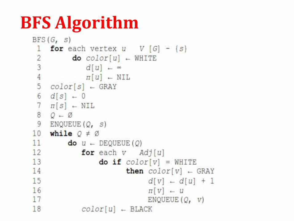
BFS Algorithm

BFS Algorithm

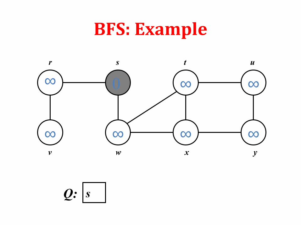
BFS: Example

∞

∞

∞

∞

∞

∞

∞

∞

r s t u

v w x y

∞

∞

0

∞

∞

∞

∞

∞

r s t u

v w x y

sQ:

BFS: Example

1

∞

0

1

∞

∞

∞

∞

r s t u

v w x y

wQ: r

BFS: Example

BFS: Example

1

∞

0

1

2

2

∞

∞

r s t u

v w x y

rQ: t x

BFS: Example

1

2

0

1

2

2

∞

∞

r s t u

v w x y

Q: t x v

BFS: Example

1

2

0

1

2

2

3

∞

r s t u

v w x y

Q: x v u

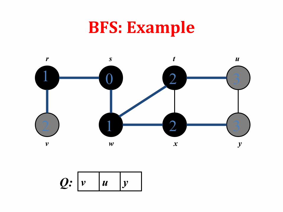
BFS: Example

1

2

0

1

2

2

3

3

r s t u

v w x y

Q: v u y

BFS: Example

1

2

0

1

2

2

3

3

r s t u

v w x y

Q: u y

BFS: Example

1

2

0

1

2

2

3

3

r s t u

v w x y

Q: y

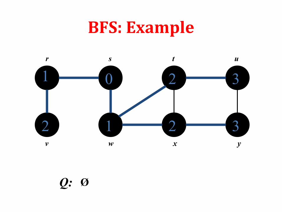
BFS: Example

1

2

0

1

2

2

3

3

r s t u

v w x y

Q: Ø

BFS: Time Complexity

Queuing time is O(V) and scanning all edges requires O(E)

Overhead for initialization is O (V) So, total running time is O(V+E)

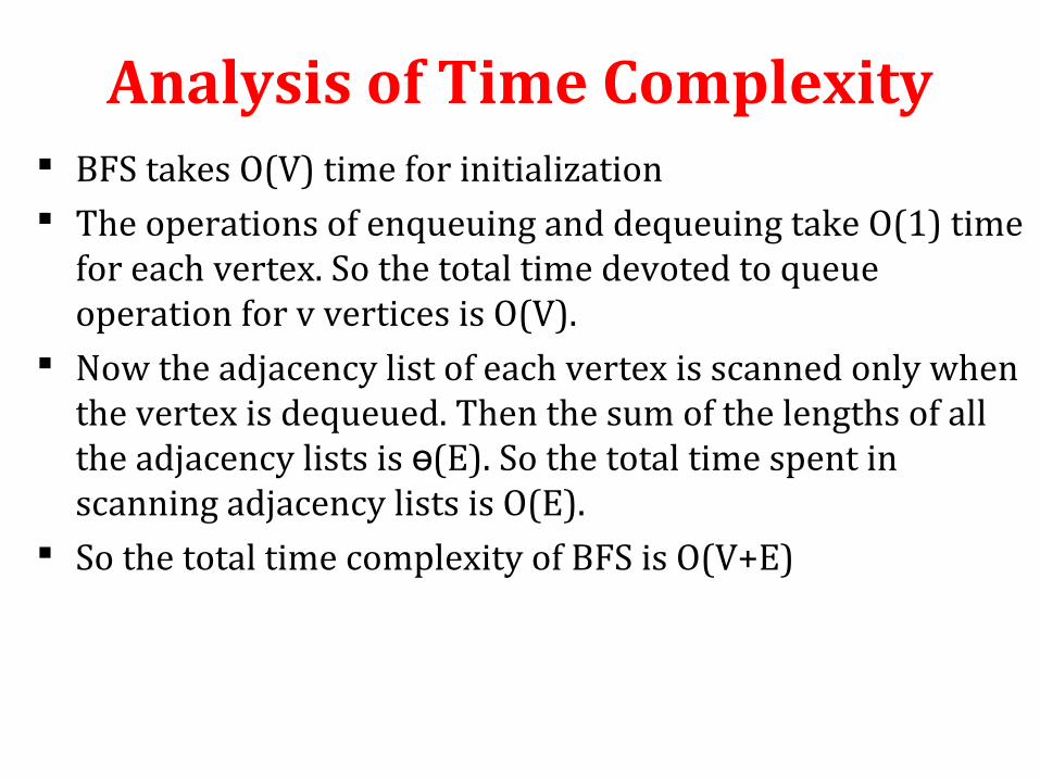
Analysis of Time Complexity BFS takes O(V) time for initialization The operations of enqueuing and dequeuing take O(1) time

for each vertex. So the total time devoted to queue operation for v vertices is O(V).

Now the adjacency list of each vertex is scanned only when the vertex is dequeued. Then the sum of the lengths of all the adjacency lists is (E). So the total time spent in ɵscanning adjacency lists is O(E).

So the total time complexity of BFS is O(V+E)

BFS: Application

• Shortest path problem

Depth First Search DFS, go as far as possible along a single path until it reaches

a dead end (that is a vertex with no edge out or no neighbor unexplored) then backtrack

As the name implies the DFS search deeper in the graph whenever possible. DFS explores edges out of the most recently discovered vertex v that still has unexplored edges leaving it. Once all of v’s edges have been explored, the search backtracks to explore edges leaving the vertex from which v was discovered.

Depth First Search To keep track of progress DFS colors each vertex white, gray or

black. Initially all the vertices are colored white. Then they are colored gray when discovered. Finally colored black when finished.

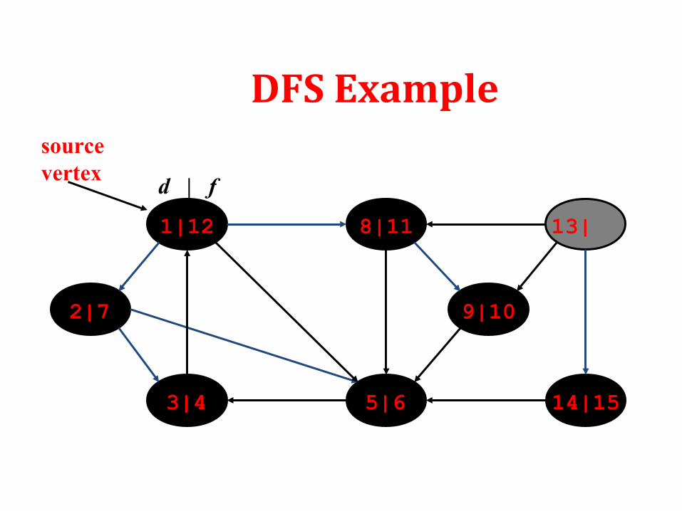
Besides creating depth first forest DFS also timestamps each vertex. Each vertex goes through two time stamps:

Discover time d[u]: when u is first discovered

Finish time f[u]: when backtrack from u or finished u

f[u] > d[u]

DFS: Algorithm DFS(G)

1. for each vertex u in G

2. color[u]=white

3. [u]=NILᴨ

4. time=0

5. for each vertex u in G

6. if (color[u]==white)

7. DFS-VISIT(G,u)

DFS-VISIT(u)

1. time = time + 1

2. d[u] = time

3. color[u]=gray

4. for each v € Adj(u) in G do

5. if (color[v] = =white)

6. [v] = u;ᴨ

7. DFS-VISIT(G,v);

8. color[u] = black

9. time = time + 1;

10. f[u]= time;

DFS: Algorithm (Cont.)

sourcevertex

DFS Examplesourcevertex

DFS Example

1 | | |

| | |

| |

sourcevertex

d | f

DFS Example

1 | | |

| | |

2 | |

sourcevertex

d | f

DFS Example

1 | | |

| | 3 |

2 | |

sourcevertex

d | f

DFS Example

1 | | |

| | 3|4

2 | |

sourcevertex

d | f

DFS Example

1 | | |

| 5 | 3|4

2 | |

sourcevertex

d | f

DFS Example

1 | | |

| 5|63|4

2 | |

sourcevertex

d | f

DFS Example

1 | | |

| 5|63|4

2|7 |

sourcevertex

d | f

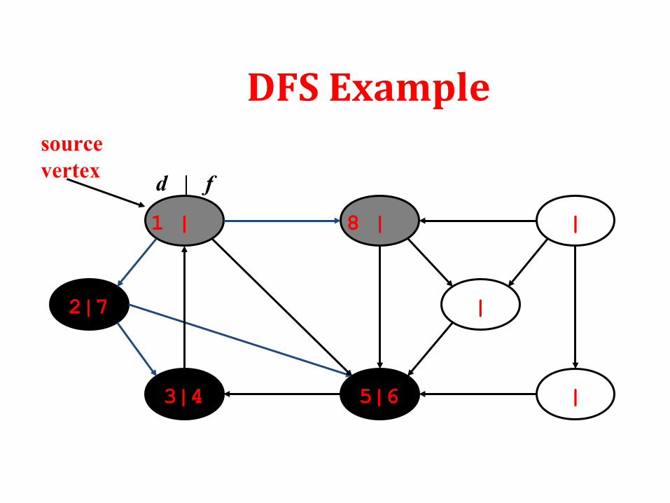
DFS Example

1 | 8 | |

| 5|63|4

2|7 |

sourcevertex

d | f

DFS Example

1 | 8 | |

| 5|63|4

2|7 9 |

sourcevertex

d | f

DFS Example

1 | 8 | |

| 5|63|4

2|7 9|10

sourcevertex

d | f

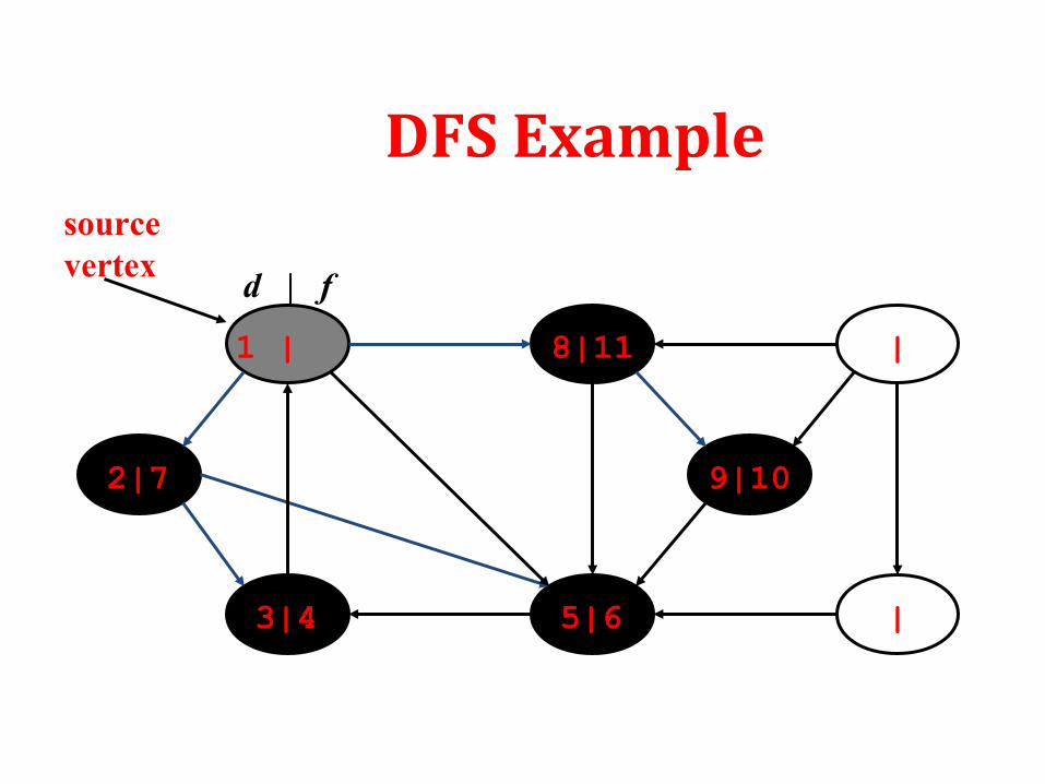
DFS Example

1 | 8|11 |

| 5|63|4

2|7 9|10

sourcevertex

d | f

DFS Example

1|12 8|11 |

| 5|63|4

2|7 9|10

sourcevertex

d | f

DFS Example

1|12 8|11 13|

| 5|63|4

2|7 9|10

sourcevertex

d | f

DFS Example

1|12 8|11 13|

14| 5|63|4

2|7 9|10

sourcevertex

d | f

DFS Example

1|12 8|11 13|

14|155|63|4

2|7 9|10

sourcevertex

d | f

DFS Example

1|12 8|11 13|16

14|155|63|4

2|7 9|10

sourcevertex

d | f

DFS: Complexity Analysis

Initialization complexity is O(V) DFS_VISIT is called exactly once for each vertex And DFS_VISIT scans all the edges which causes

cost of O(E) Thus overall complexity is O(V + E)

DFS: Application

• Topological Sort• Strongly Connected Component

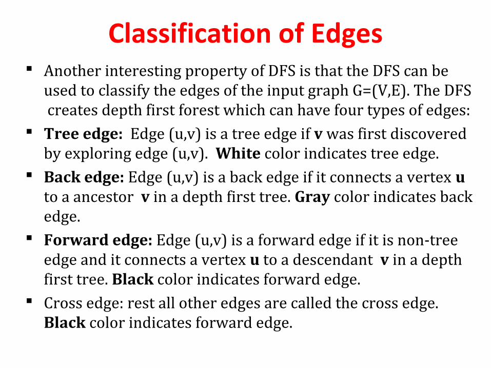
Classification of Edges Another interesting property of DFS is that the DFS can be

used to classify the edges of the input graph G=(V,E). The DFS creates depth first forest which can have four types of edges:

Tree edge: Edge (u,v) is a tree edge if v was first discovered by exploring edge (u,v). White color indicates tree edge.

Back edge: Edge (u,v) is a back edge if it connects a vertex u to a ancestor v in a depth first tree. Gray color indicates back edge.

Forward edge: Edge (u,v) is a forward edge if it is non-tree edge and it connects a vertex u to a descendant v in a depth first tree. Black color indicates forward edge.

Cross edge: rest all other edges are called the cross edge. Black color indicates forward edge.

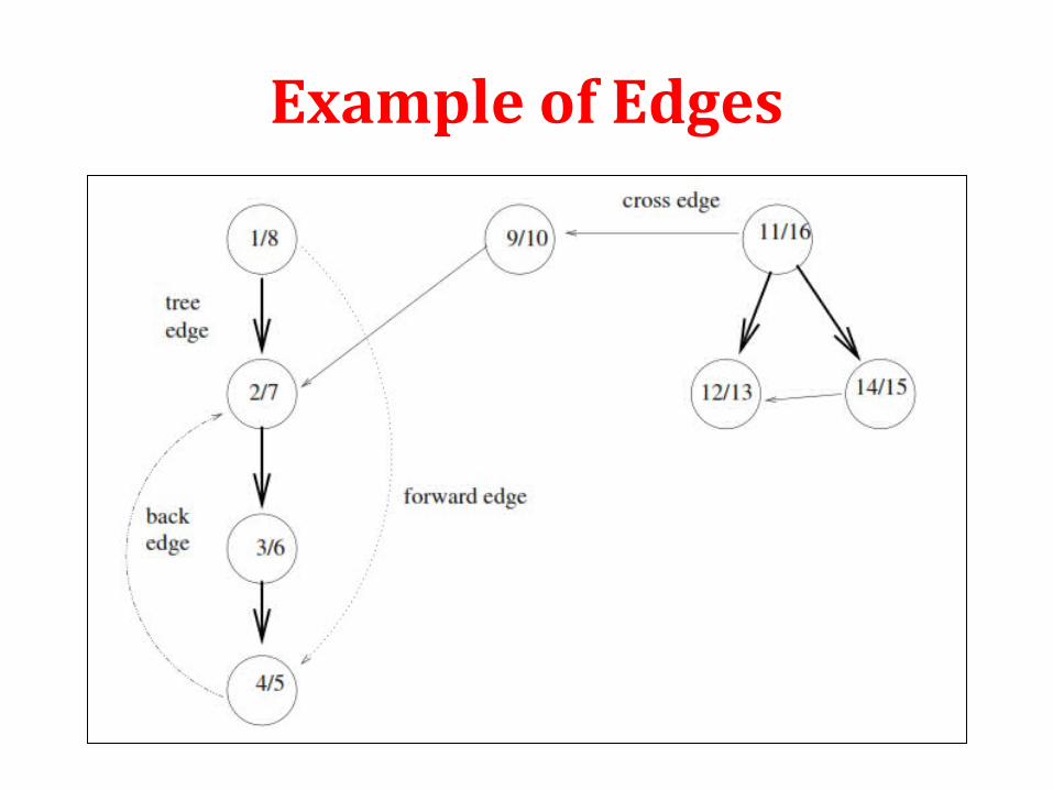
Example of Edges

Theorem Derived from DFS

Theorem 1: In a depth first search of an undirected graph G, every edge of G is either a tree edge or back edge.

Theorem 2: A directed graph G is acyclic if and only if a depth-first search of G yields no back edges.

Container of BFS and DFS

Choice of container used to store discovered vertices while graph search…

If a queue is used as the container, we get breadth first search.

If a stack is used as the container, we get depth first search.

Problem to Solve

Mawa

Dhaka

Majir Ghat

Jajira

Shariatpur

Naria

BhederGong

University

MD. Shakhawat Hossain Student of Computer Science & Engineering Dept.

University of Rajshahi