brandon growth forecast final report · brandon growth forecast final report ... total industrial...

Brandon Growth Forecast Final Report

Prepared For the City of Brandon

March 5, 2017

SJ Research Services 3004 College Avenue Regina, Saskatchewan S4T 2V8 Phone: (306) 539-4320 Email: [email protected]

Schedule J

mailto:[email protected]

2 | P a g e

Table of Contents

Executive Summary ........................................................................................................................... 3

Methodology ..................................................................................................................................... 4

The Base Case Forecast .............................................................................................................. 5

The High Growth Forecast .......................................................................................................... 9

Population Forecast .................................................................................................................. 13

Appendix A: Developing Community Level Input-output models .................................................. 18

List of Tables Table 1: New Land Requirements per year in Hectares (vs.2015) Base Case City of Brandon and RMs by Aggregated Sector ............................................................................ 3 Table 2: New Land Requirements per year in Hectares (vs.2015) High Growth City of Brandon and RMs by Aggregated Sector ............................................................................ 3 Table 3: Housing Starts City of Brandon and Surrounding RMs ......................................... 3 Table 4: Industry Detail: Brandon Economic Model ........................................................... 4 Table 5: Constant Dollar Gross Domestic Product by Industry (2007 $M) – Base Case Forecast ............................................................................................................................... 5 Table 6: Employment by Industry – Base Case Forecast .................................................... 6 Table 7: New Land Requirements per year in Hectares (vs.2015) Base Case .................... 7 Table 8: Industry Distribution-Industrial, Commercial, and Institutional ........................... 8 Table 9: New Land Requirements per year in Hectares (vs.2015) Base Case City of Brandon and RMs by Aggregated Sector ............................................................................ 9 Table 10: High Growth Scenario Assumptions ................................................................. 10 Table 11: Constant Dollar Gross Domestic Product by Industry (2007 $M) – High Growth Forecast ............................................................................................................................. 10 Table 12: Employment by Industry – High Growth Forecast ............................................ 11 Table 13: New Land Requirements per year in Hectares (vs.2015) High Growth ............ 12 Table 14: New Land Requirements per year in Hectares (vs.2015) High Growth City of Brandon and RMs by Aggregated Sector .......................................................................... 13 Table 15: Population Forecast Base Case ......................................................................... 14 Table 16: Population Forecast High Growth ..................................................................... 15 Table 17: Population forecast Breakdown City of Brandon vs. Surrounding RMs ........... 16 Table 18: Housing Starts-City of Brandon vs. Surrounding RMs. ..................................... 17

3 | P a g e

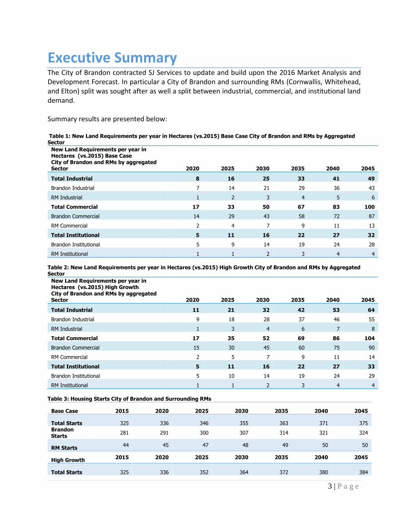
Executive Summary The City of Brandon contracted SJ Services to update and build upon the 2016 Market Analysis and Development Forecast. In particular a City of Brandon and surrounding RMs (Cornwallis, Whitehead, and Elton) split was sought after as well a split between industrial, commercial, and institutional land demand. Summary results are presented below: Table 1: New Land Requirements per year in Hectares (vs.2015) Base Case City of Brandon and RMs by Aggregated Sector

New Land Requirements per year in Hectares (vs.2015) Base Case City of Brandon and RMs by aggregated Sector 2020 2025 2030 2035 2040 2045

Total Industrial 8 16 25 33 41 49

Brandon Industrial 7 14 21 29 36 43

RM Industrial 1 2 3 4 5 6

Total Commercial 17 33 50 67 83 100

Brandon Commercial 14 29 43 58 72 87

RM Commercial 2 4 7 9 11 13

Total Institutional 5 11 16 22 27 32

Brandon Institutional 5 9 14 19 24 28

RM Institutional 1 1 2 3 4 4

Table 2: New Land Requirements per year in Hectares (vs.2015) High Growth City of Brandon and RMs by Aggregated Sector

New Land Requirements per year in Hectares (vs.2015) High Growth City of Brandon and RMs by aggregated Sector 2020 2025 2030 2035 2040 2045










Table 3: Housing Starts City of Brandon and Surrounding RMs

Base Case 2015 2020 2025 2030 2035 2040 2045

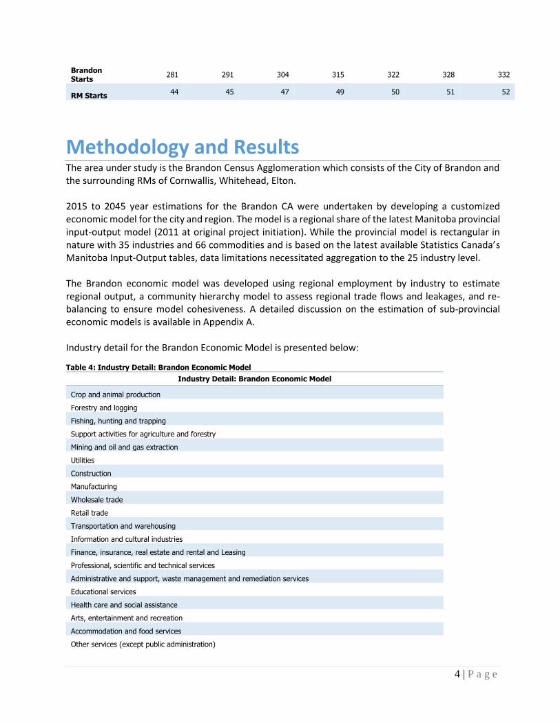
Total Starts 325 336 346 355 363 371 375 Brandon Starts

281 291 300 307 314 321 324

RM Starts 44 45 47 48 49 50 50

High Growth 2015 2020 2025 2030 2035 2040 2045

Total Starts 325 336 352 364 372 380 384

4 | P a g e

Brandon Starts

281 291 304 315 322 328 332

RM Starts 44 45 47 49 50 51 52

Methodology and Results The area under study is the Brandon Census Agglomeration which consists of the City of Brandon and the surrounding RMs of Cornwallis, Whitehead, Elton. 2015 to 2045 year estimations for the Brandon CA were undertaken by developing a customized economic model for the city and region. The model is a regional share of the latest Manitoba provincial input-output model (2011 at original project initiation). While the provincial model is rectangular in nature with 35 industries and 66 commodities and is based on the latest available Statistics Canada’s Manitoba Input-Output tables, data limitations necessitated aggregation to the 25 industry level. The Brandon economic model was developed using regional employment by industry to estimate regional output, a community hierarchy model to assess regional trade flows and leakages, and re-balancing to ensure model cohesiveness. A detailed discussion on the estimation of sub-provincial economic models is available in Appendix A. Industry detail for the Brandon Economic Model is presented below: Table 4: Industry Detail: Brandon Economic Model

Industry Detail: Brandon Economic Model

Crop and animal production

Forestry and logging

Fishing, hunting and trapping

Support activities for agriculture and forestry

Mining and oil and gas extraction

Utilities

Construction

Manufacturing

Wholesale trade

Retail trade

Transportation and warehousing

Information and cultural industries

Finance, insurance, real estate and rental and Leasing

Professional, scientific and technical services

Administrative and support, waste management and remediation services

Educational services

Health care and social assistance

Arts, entertainment and recreation

Accommodation and food services

Other services (except public administration)

5 | P a g e

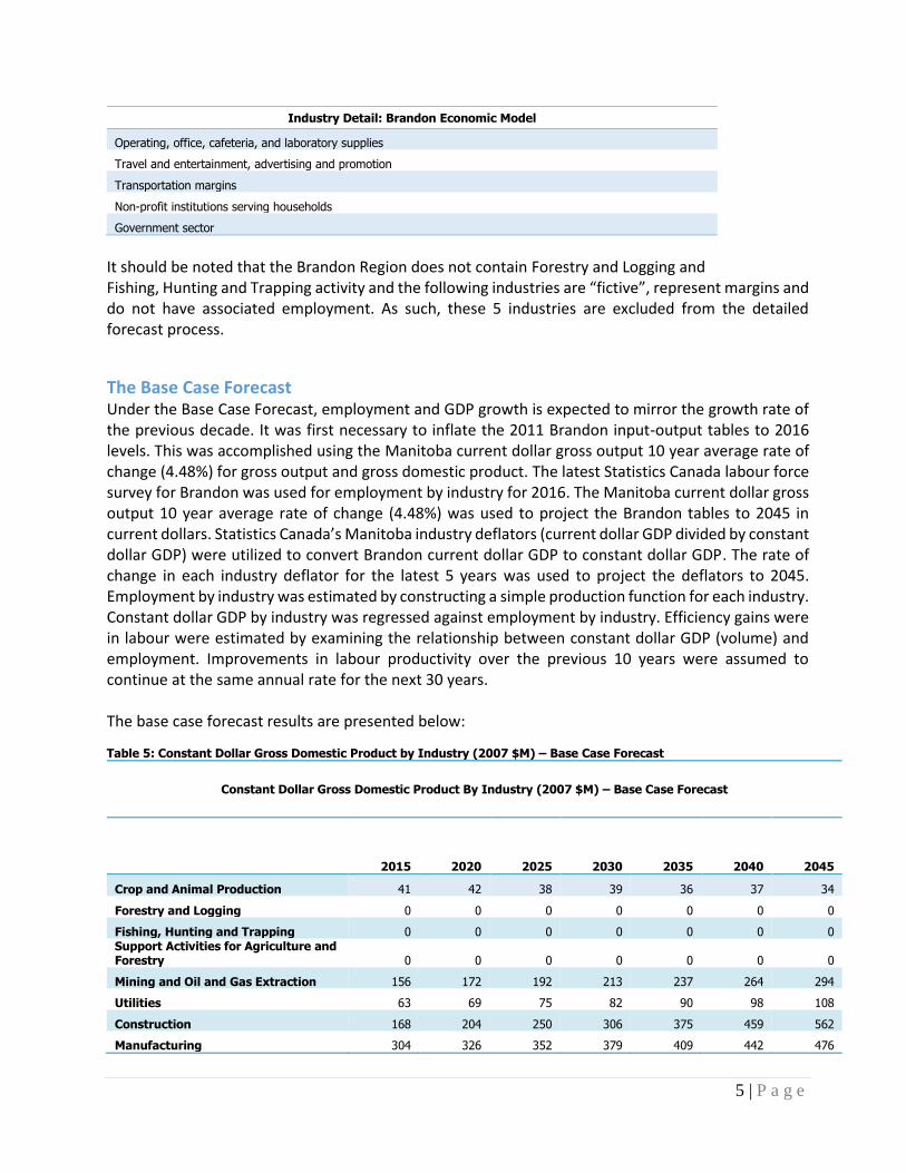
Industry Detail: Brandon Economic Model

Operating, office, cafeteria, and laboratory supplies

Travel and entertainment, advertising and promotion

Transportation margins

Non-profit institutions serving households

Government sector

It should be noted that the Brandon Region does not contain Forestry and Logging and Fishing, Hunting and Trapping activity and the following industries are “fictive”, represent margins and do not have associated employment. As such, these 5 industries are excluded from the detailed forecast process.

The Base Case Forecast Under the Base Case Forecast, employment and GDP growth is expected to mirror the growth rate of the previous decade. It was first necessary to inflate the 2011 Brandon input-output tables to 2016 levels. This was accomplished using the Manitoba current dollar gross output 10 year average rate of change (4.48%) for gross output and gross domestic product. The latest Statistics Canada labour force survey for Brandon was used for employment by industry for 2016. The Manitoba current dollar gross output 10 year average rate of change (4.48%) was used to project the Brandon tables to 2045 in current dollars. Statistics Canada’s Manitoba industry deflators (current dollar GDP divided by constant dollar GDP) were utilized to convert Brandon current dollar GDP to constant dollar GDP. The rate of change in each industry deflator for the latest 5 years was used to project the deflators to 2045. Employment by industry was estimated by constructing a simple production function for each industry. Constant dollar GDP by industry was regressed against employment by industry. Efficiency gains were in labour were estimated by examining the relationship between constant dollar GDP (volume) and employment. Improvements in labour productivity over the previous 10 years were assumed to continue at the same annual rate for the next 30 years. The base case forecast results are presented below: Table 5: Constant Dollar Gross Domestic Product by Industry (2007 $M) – Base Case Forecast

Constant Dollar Gross Domestic Product By Industry (2007 $M) – Base Case Forecast

2015 2020 2025 2030 2035 2040 2045

Crop and Animal Production 41 42 38 39 36 37 34

Forestry and Logging 0 0 0 0 0 0 0

Fishing, Hunting and Trapping 0 0 0 0 0 0 0 Support Activities for Agriculture and Forestry 0 0 0 0 0 0 0

Mining and Oil and Gas Extraction 156 172 192 213 237 264 294

Utilities 63 69 75 82 90 98 108

Construction 168 204 250 306 375 459 562

Manufacturing 304 326 352 379 409 442 476

6 | P a g e

Constant Dollar Gross Domestic Product By Industry (2007 $M) – Base Case Forecast

2015 2020 2025 2030 2035 2040 2045

Wholesale Trade 116 136 160 188 222 262 309

Retail Trade 207 240 281 327 382 446 520

Transportation and Warehousing 104 122 144 169 199 235 277

Information and Cultural Industries 123 142 166 193 225 262 306 Finance, Insurance, Real Estate and Rental and Leasing 362 424 500 589 695 819 965 Professional, Scientific and Technical Services 58 65 73 83 93 105 118 Administrative and Support, Waste Management and Remediation Services 36 39 43 47 51 56 61

Educational Services 3 3 4 4 5 5 6

Health Care and Social Assistance 65 85 91 120 127 168 179

Arts, Entertainment and Recreation 16 18 20 22 24 26 28

Accommodation and Food Services 62 74 88 105 126 151 180 Other Services (Except Public Administration) 23 25 27 30 32 36 39 Operating, Office, Cafeteria and Laboratory Supplies 0 0 0 0 0 0 0 Travel, Entertainment, Advertising and Promotion 0 0 0 0 0 0 0

Transportation Margins 0 0 0 0 0 0 0 Non-Profit Institutions Serving Households 30 33 36 39 43 47 52

Government Sector 793 893 1012 1145 1297 1469 1663

Total 2729 3113 3550 4083 4670 5386 6177

Table 6: Employment by Industry – Base Case Forecast

Employment By Industry – Base Case Forecast

2015 2020 2025 2030 2035 2040 2045





Utilities 302 309 316 323 330 337 344

Construction 1,879 2,119 2,359 2,599 2,838 3,078 3,318

Manufacturing 2,886 3,034 3,181 3,329 3,476 3,624 3,771

Wholesale Trade 844 911 978 1,045 1,113 1,180 1,247

Retail Trade 3,735 4,091 4,448 4,804 5,161 5,517 5,873

Transportation and Warehousing 1,040 1,157 1,274 1,391 1,508 1,625 1,742

7 | P a g e

Employment By Industry – Base Case Forecast

2015 2020 2025 2030 2035 2040 2045

Information and Cultural Industries 532 597 663 728 793 858 924 Finance, Insurance, Real Estate and Rental and Leasing 1,213 1,344 1,474 1,605 1,735 1,866 1,996 Professional, Scientific and Technical Services 676 714 751 789 827 864 902 Administrative and Support, Waste Management and Remediation Services 681 730 780 830 880 929 979


Health Care and Social Assistance 920 1,011 1,102 1,193 1,284 1,375 1,466


Accommodation and Food Services 2,177 2,433 2,690 2,947 3,203 3,460 3,716 Other Services (Except Public Administration) 575 597 618 640 661 683 704 Operating, Office, Cafeteria and Laboratory Supplies 0 0 0 0 0 0 0 Travel, Entertainment, Advertising and Promotion 0 0 0 0 0 0 0


Government Sector 9,190 10,003 10,816 11,628 12,441 13,254 14,066

Total 28,700 31,101 33,503 35,904 38,306 40,707 43,109

Land use requirements were based on a similar study conducted for the city of Edmonton. This study estimated floor area requirements per employee across 13 industries. Projected demand figures were then translated into land area requirements using site coverage ratios typical for each industry. Site coverage constitutes the percentage of a site that is covered by the built environment. Base case land requirements by industry are presented below: Table 7: New Land Requirements per year in Hectares (vs.2015) Base Case

New Land Requirements per year in Hectares (vs.2015) Base Case

2020 2025 2030 2035 2040 2045

Crop and Animal Production 0 0 0 0 0 0

Forestry and Logging 0 0 0 0 0 0

Fishing, Hunting and Trapping 0 0 0 0 0 0 Support Activities for Agriculture and Forestry 0 0 0 0 0 0

Mining and Oil and Gas Extraction 0 0 0 0 0 0

Utilities 0 0 0 1 1 1

Construction 5 10 16 21 26 31

Manufacturing 3 6 8 11 14 17

Wholesale Trade 1 3 4 5 7 8

8 | P a g e

New Land Requirements per year in Hectares (vs.2015) Base Case

2020 2025 2030 2035 2040 2045

Retail Trade 7 14 21 28 35 42

Transportation and Warehousing 4 8 11 15 19 23

Information and Cultural Industries 0 0 1 1 1 1 Finance, Insurance, Real Estate and Rental and Leasing 0 1 1 2 2 3 Professional, Scientific and Technical Services 0 0 0 0 1 1 Administrative and Support, Waste Management and Remediation Services 0 0 0 1 1 1

Educational Services 0 0 0 0 1 1

Health Care and Social Assistance 1 2 2 3 4 5

Arts, Entertainment and Recreation 0 0 1 1 1 1

Accommodation and Food Services 2 5 7 9 12 14 Other Services (Except Public Administration) 0 0 1 1 1 1 Operating, Office, Cafeteria and Laboratory Supplies 0 0 0 0 0 0 Travel, Entertainment, Advertising and Promotion 0 0 0 0 0 0

Transportation Margins 0 0 0 0 0 0 Non-Profit Institutions Serving Households 0 0 0 1 1 1

Government Sector 5 11 16 21 26 32

Total 30 61 91 121 152 182

Results were aggregated into the larger components of industrial, commercial, and institutional based on the following industry distribution: Table 8: Industry Distribution-Industrial, Commercial, and Institutional

Industry Distribution: Industrial, Commercial, and Institutional

Crop and animal production Industrial

Forestry and logging NA

Fishing, hunting and trapping NA

Support activities for agriculture and forestry Industrial

Mining and oil and gas extraction Industrial

Utilities Industrial

Construction Industrial

Manufacturing Industrial

Wholesale trade Commercial

Retail trade Commercial

Transportation and warehousing Commercial

Information and cultural industries Commercial

Finance, insurance, real estate and rental and Leasing Commercial

Professional, scientific and technical services Commercial

Administrative and support, waste management and remediation services Commercial

Educational services Commercial

9 | P a g e

Industry Distribution: Industrial, Commercial, and Institutional

Health care and social assistance Commercial

Arts, entertainment and recreation Commercial

Accommodation and food services Commercial

Other services (except public administration) Commercial

Operating, office, cafeteria, and laboratory supplies NA

Travel and entertainment, advertising and promotion NA

Transportation margins NA

Non-profit institutions serving households Institutional

Government sector Institutional

Aggregated results were, in turn, allocated between the City of Brandon and the surrounding RMs based on the employment by industry split between industrial, commercial, and institutional sectors in Brandon relative to the RMs. Data for this exercise was available in the 2011 Statistics Canada National Household Survey, the latest available. The resulting disaggregation is below: Table 9: New Land Requirements per year in Hectares (vs.2015) Base Case City of Brandon and RMs by Aggregated Sector

New Land Requirements per year in Hectares (vs.2015) Base Case City of Brandon and RMs by Aggregated Sector 2020 2025 2030 2035 2040 2045










The High Growth Forecast A series of exogenous shocks (output and investment) to the Bandon economy over the next 30 years generated industry employment and output results over and above the base case results.

The high growth scenario was based on the following model inputs:

10 | P a g e

Table 10: High Growth Scenario Assumptions

Construction periods were based on the mid-point year in the range and assumed a 1 year construction period was assumed. The actual manufacturing begins the next year. Construction impacts are one-time and manufacturing impacts are on-going. Model generated indirect and induced employment are included in the results. Indirect impacts measure the secondary business transactions that result from the initial expenditures. Induced impacts are third round impacts from the spending of incremental labour income in the economy after removing a portion for taxes and savings. The discrepancies between GDP and employment impacts in the high growth scenario are due to the addition of plants producing hundreds of millions in new output with only 15 to 40 new employees.

High growth forecast results are presented below: Table 11: Constant Dollar Gross Domestic Product by Industry (2007 $M) – High Growth Forecast

Constant Dollar Gross Domestic Product By Industry (2007 $M) – High Growth Forecast

2015 2020 2025 2030 2035 2040 2045





Utilities 63 69 75 84 92 100 109

Construction 168 208 271 307 376 460 563

Manufacturing 304 326 376 584 587 597 611

Wholesale Trade 116 136 160 192 225 265 311

Retail Trade 207 241 281 328 382 446 521

Transportation and Warehousing 104 122 144 174 204 240 281

Estimated timing

Assumed Construction Year

Construction Cost ($M)

Annual Incremental Output ($M)

New Employment

Soybean processing 600,000 ton/yr (mechanical) 5 to 10 yrs 2022 60 70 40

Soybean Bio-Diesel 20 to 100 million litre 10 to 15 yrs 2028 20 50 15

Ethanol and Distiller Grains Production Plant 15 to 25 yrs 2025 70 100 30 Food Grade Oil, Tallow and Meat Co-Products

Processing Plant 10 to 30 years 2035 na na na

Food Cluster 80 firms 5 to 10 yrs

begins in 2020

complete in 2024 3M/year 28 550

Federal Infrastructure Program 0 to 10 years

Begins in 2016

complete is 2025 13M/year na 148

Reinvigorated Hog Sector 0 to 15 years 2023 38 6.5 0

11 | P a g e

Constant Dollar Gross Domestic Product By Industry (2007 $M) – High Growth Forecast

2015 2020 2025 2030 2035 2040 2045

Information and Cultural Industries 123 142 166 196 228 265 308 Finance, Insurance, Real Estate and Rental and Leasing 362 424 500 591 696 820 967 Professional, Scientific and Technical Services 58 65 74 84 95 106 119 Administrative and Support, Waste Management and Remediation Services 36 39 43 48 52 57 62


Health Care and Social Assistance 65 85 91 120 128 169 179


Accommodation and Food Services 62 74 88 105 126 151 180 Other Services (Except Public Administration) 23 25 27 30 32 36 39 Operating, Office, Cafeteria and Laboratory Supplies 0 0 0 0 0 0 0 Travel, Entertainment, Advertising and Promotion 0 0 0 0 0 0 0


Government Sector 793 893 1012 1148 1299 1470 1664

Total 2729 3614 4538 5951 7274 8914 10945

Table 12: Employment by Industry – High Growth Forecast

Employment By Industry – High Growth Forecast

2015 2020 2025 2030 2035 2040 2045





Utilities 302 312 322 332 342 352 362

Construction 1,879 2,122 2,364 2,606 2,848 3,090 3,333

Manufacturing 2,886 3,146 3,406 3,666 3,926 4,186 4,446

Wholesale Trade 844 917 990 1,063 1,136 1,209 1,282

Retail Trade 3,735 4,092 4,449 4,806 5,163 5,520 5,877

Transportation and Warehousing 1,040 1,170 1,299 1,429 1,559 1,688 1,818

Information and Cultural Industries 532 601 669 737 805 874 942 Finance, Insurance, Real Estate and Rental and Leasing 1,213 1,345 1,477 1,609 1,741 1,874 2,006

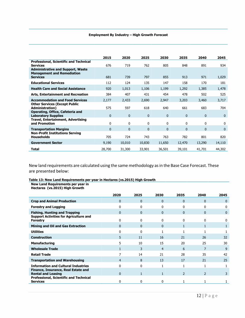
12 | P a g e

Employment By Industry – High Growth Forecast

2015 2020 2025 2030 2035 2040 2045 Professional, Scientific and Technical Services 676 719 762 805 848 891 934 Administrative and Support, Waste Management and Remediation Services 681 739 797 855 913 971 1,029


Health Care and Social Assistance 920 1,013 1,106 1,199 1,292 1,385 1,478


Accommodation and Food Services 2,177 2,433 2,690 2,947 3,203 3,460 3,717 Other Services (Except Public Administration) 575 597 618 640 661 683 704 Operating, Office, Cafeteria and Laboratory Supplies 0 0 0 0 0 0 0 Travel, Entertainment, Advertising and Promotion 0 0 0 0 0 0 0


Government Sector 9,190 10,010 10,830 11,650 12,470 13,290 14,110

Total 28,700 31,300 33,901 36,501 39,101 41,701 44,302

New land requirements are calculated using the same methodology as in the Base Case Forecast. These are presented below: Table 13: New Land Requirements per year in Hectares (vs.2015) High Growth

New Land Requirements per year in Hectares (vs.2015) High Growth

2020 2025 2030 2035 2040 2045

Crop and Animal Production 0 0 0 0 0 0

Forestry and Logging 0 0 0 0 0 0

Fishing, Hunting and Trapping 0 0 0 0 0 0 Support Activities for Agriculture and Forestry 0 0 0 0 0 0

Mining and Oil and Gas Extraction 0 0 0 1 1 1

Utilities 0 0 1 1 1 1

Construction 5 11 16 21 26 32

Manufacturing 5 10 15 20 25 30

Wholesale Trade 1 3 4 6 7 9

Retail Trade 7 14 21 28 35 42

Transportation and Warehousing 4 8 13 17 21 25

Information and Cultural Industries 0 0 1 1 1 1 Finance, Insurance, Real Estate and Rental and Leasing 0 1 1 2 2 3 Professional, Scientific and Technical Services 0 0 0 1 1 1

13 | P a g e

New Land Requirements per year in Hectares (vs.2015) High Growth

2020 2025 2030 2035 2040 2045 Administrative and Support, Waste Management and Remediation Services 0 0 1 1 1 1

Educational Services 0 0 0 0 1 1

Health Care and Social Assistance 1 2 3 3 4 5

Arts, Entertainment and Recreation 0 0 1 1 1 1

Accommodation and Food Services 2 5 7 9 12 14 Other Services (Except Public Administration) 0 0 1 1 1 1 Operating, Office, Cafeteria and Laboratory Supplies 0 0 0 0 0 0 Travel, Entertainment, Advertising and Promotion 0 0 0 0 0 0

Transportation Margins 0 0 0 0 0 0 Non-Profit Institutions Serving Households 0 0 1 1 1 1

Government Sector 5 11 16 21 27 32

Total 33 67 100 133 167 200

A similar sector aggregation and regional breakdown was conducted with the high growth forecast: Table 14: New Land Requirements per year in Hectares (vs.2015) High Growth City of Brandon and RMs by Aggregated Sector

New Land Requirements per year in Hectares (vs.2015) High Growth City of Brandon and RMs by aggregated Sector 2020 2025 2030 2035 2040 2045










Population Forecast The population model is a simple cohort survival model using birth and death rates and migration data from Statistics Canada. In its basic form, a cohort-survival model estimates future population based on the previous period’s population plus natural increase (births less deaths) and net migration: Population[t+1] = Population[t] + Natural Increase + Net Migration This is calculated for men and women for each age-group. The time interval is determined by the age cohorts. The smallest time interval for which an estimate can be made is the length of time it takes all the members of an age cohort (e.g., age 10 - 14) to pass on to the next age grouping (e.g., the 15 - 19 year-old group). All of the cohorts must be the same dimension (e.g., 5-year increments, 7-year

14 | P a g e

increments), since over the course of the analysis each group must pass from one cohort to the next. All estimates must use time-intervals which are multiples of the cohort size. Natural increase is the difference between the number of children born and the number of people who die during one time interval. The analysis, however, is being done in terms of age-cohorts for each sex. Children can only be born into the first cohort but people die in all of the cohorts (including the birth cohort). Further, the number of males has no direct effect on the number of children born. Children are born only to women of childbearing age based on historical births per female population by age group. Deaths by age group are also based on historical deaths per age group population. Migration, both in and out, includes international, inter-provincial, and intra-provincial. Migration data is largely unavailable for the region. However, migration data is readily available for Statistics Canada’s Manitoba Census Divisions (CD) 7 which contains the bulk of the population (including Brandon) of the region. The proportion of the region to CD population times the migration data was assumed to represent in and out migration for the region, and the average of the latest 5 years available was used to predict future baseline migration. Additional in-migration from the high growth scenario was added to the base case in-migration. The latest Manitoba birth rate by age of mother, death rate by age and gender, and propensity to in and out migrate by age group and gender from Statistic Canada were used for both the base case and high growth population forecast. Finally, 2011 census population was used as the starting point. Because this exercise is designed to measuring incremental impacts rather than an entire population count, these further assumptions were used as the basis for analysis:

Migration is driven labour demand and demand for indirect and induced construction employment is assumed to follow the same peak as construction.

Based on previous large scale resource projects, it can be assumed that 10% of the regional construction workforce (excluding indirect and induced) will relocate permanently to the region.

Among those that in-migrate to the region, it can be expected that those earning higher wages will in-migrate with families. To model this, it is assumed that in-migrants will bring an average household to the region of 2.42 (regional population divided by number of households from latest Statistics Canada census) if the industry where demand occurs has an average wage higher than the provincial average. In this case new migration is broken down by age and gender by the age/gender split in the region. Where the industry average wage is below the provincial average, in-migrants will be single in-migrants and will be broken down by age and gender by the age and gender split of the region 20-64 (working age) age group.

With 1,720 unemployed and an unemployment rate of 5.6%, current labour demand requirements will be met through the current levels of in-migration, new local entrants into the labour market, and 10% of the available local labour for having the skills required to meet future demand. This is the case until 2023-2024 when labour demand exceeds local labour force and in-migration availability.

Table 15: Population Forecast Base Case

Population Forecast Base Case

2015 2020 2025 2030 2035 2040 2045

0-4 3,741 4,030 3,988 3,886 3,918 4,039 4,079

15 | P a g e

Population Forecast Base Case

2015 2020 2025 2030 2035 2040 2045

5-9 3,688 3,856 4,145 4,103 4,001 4,033 4,106

10-14 3,354 3,814 3,981 4,270 4,228 4,126 4,160

15-19 3,292 3,560 4,018 4,186 4,473 4,432 4,447

20-24 3,582 3,250 3,517 3,973 4,140 4,426 4,474

25-29 4,893 3,939 3,608 3,874 4,328 4,495 4,689

30-34 4,351 5,174 4,224 3,895 4,159 4,612 4,660

35-39 4,020 4,332 5,152 4,206 3,878 4,141 4,236

40-44 3,623 4,048 4,359 5,173 4,233 3,908 3,908

45-49 3,265 3,648 4,069 4,376 5,180 4,251 4,046

50-54 3,591 3,213 3,589 4,003 4,305 5,095 5,188

55-59 3,360 3,446 3,075 3,442 3,848 4,144 4,485

60-64 2,897 3,283 3,365 3,006 3,361 3,754 3,753

65-69 2,569 2,877 3,245 3,324 2,980 3,318 3,426

70-74 1,752 2,400 2,684 3,026 3,098 2,778 2,752

75-79 1,371 1,530 2,093 2,336 2,635 2,695 2,727

80-84 1,010 1,039 1,166 1,605 1,790 2,025 2,120

85-89 719 645 665 750 1,035 1,151 1,225

90+ 558 606 588 590 635 793 855

Total 55,638 58,692 61,532 64,022 66,225 68,213 69,334

Table 16: Population Forecast High Growth

Population Forecast High Growth

2015 2020 2025 2030 2035 2040 2045

0-4 3,741 4,030 4,068 3,986 4,025 4,156 4,196

5-9 3,688 3,856 4,234 4,233 4,101 4,140 4,216

10-14 3,354 3,814 4,083 4,415 4,357 4,225 4,260

15-19 3,292 3,560 4,125 4,348 4,618 4,560 4,569

20-24 3,582 3,250 3,598 4,145 4,302 4,571 4,615

25-29 4,893 3,939 3,646 4,008 4,500 4,656 4,847

30-34 4,351 5,174 4,298 3,984 4,292 4,783 4,828

35-39 4,020 4,332 5,232 4,344 3,967 4,274 4,380

40-44 3,623 4,048 4,468 5,332 4,370 3,996 4,001

45-49 3,265 3,648 4,198 4,585 5,338 4,386 4,173

50-54 3,591 3,213 3,704 4,231 4,510 5,250 5,337

55-59 3,360 3,446 3,172 3,641 4,071 4,344 4,676

60-64 2,897 3,283 3,443 3,170 3,554 3,970 3,967

65-69 2,569 2,877 3,313 3,447 3,137 3,502 3,614

70-74 1,752 2,400 2,748 3,126 3,213 2,923 2,902

75-79 1,371 1,530 2,152 2,425 2,722 2,795 2,833

80-84 1,010 1,039 1,211 1,678 1,860 2,092 2,189

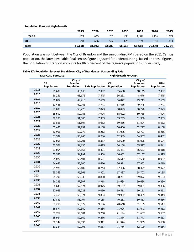
16 | P a g e

Population Forecast High Growth

2015 2020 2025 2030 2035 2040 2045

85-89 719 645 705 799 1,082 1,196 1,269

90+ 558 606 592 620 671 831 893

Total 55,638 58,692 62,989 66,517 68,688 70,648 71,764

Population was split between the City of Brandon and the surrounding RMs based on the 2011 Census population, the latest available final census figure adjusted for undercounting. Based on these figures, the population of Brandon accounts for 86.5 percent of the region’s populations under study. Table 17: Population forecast Breakdown City of Brandon vs. Surrounding RMs

Base Case Forecast High Growth Forecast

CA Population

City of Brandon

Population RMs Population CA Population

City of Brandon

Population RMs

Population

2015 55,638 48,145 7,492 55,638 48,145 7,492

2016 56,251 48,676 7,575 56,251 48,676 7,575

2017 56,872 49,213 7,659 56,872 49,213 7,659

2018 57,486 49,745 7,741 57,486 49,745 7,741

2019 58,093 50,270 7,823 58,093 50,270 7,823

2020 58,692 50,788 7,904 58,692 50,788 7,904

2021 59,283 51,300 7,983 59,283 51,300 7,983

2022 59,866 51,804 8,062 59,866 51,804 8,062

2023 60,436 52,297 8,138 60,436 52,297 8,138

2024 60,991 52,778 8,213 61,006 52,791 8,215

2025 61,532 53,246 8,286 62,989 54,507 8,482

2026 62,058 53,701 8,357 63,670 55,096 8,574

2027 62,561 54,136 8,425 64,168 55,527 8,641

2028 63,054 54,563 8,491 65,481 56,663 8,818

2029 63,550 54,992 8,558 66,052 57,157 8,895

2030 64,022 55,401 8,621 66,517 57,560 8,957

2031 64,483 55,800 8,684 66,971 57,952 9,019

2032 64,925 56,182 8,743 67,406 58,329 9,077

2033 65,363 56,561 8,802 67,837 58,702 9,135

2034 65,796 56,936 8,860 68,264 59,072 9,193

2035 66,225 57,307 8,918 68,688 59,438 9,250

2036 66,649 57,674 8,975 69,107 59,801 9,306

2037 67,059 58,028 9,030 69,511 60,151 9,361

2038 67,455 58,371 9,084 69,902 60,489 9,413

2039 67,839 58,704 9,135 70,281 60,817 9,464

2040 68,213 59,027 9,186 70,648 61,135 9,514

2041 68,574 59,340 9,234 71,004 61,442 9,562

2042 68,764 59,504 9,260 71,194 61,607 9,587

2043 68,954 59,669 9,286 71,384 61,771 9,613

2044 69,144 59,833 9,311 71,574 61,935 9,638

2045 69,334 59,998 9,337 71,764 62,100 9,664

17 | P a g e

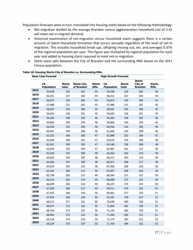
Population forecasts were in turn, translated into housing starts based on the following methodology:

Net migration divided by the average Brandon census agglomeration household size of 2.42 will meet net-in-migrant demand.

Historical examination of net-migration versus household starts suggests there is a certain amount of latent household formation that occurs annually regardless of the level of net-in migration. This includes household break ups, offspring moving out, etc. and averages 0.37% of the regional population per year. This figure was multiplied by regional population for each year and added to housing starts required to meet net-in migration.

Starts were split between the City of Brandon and the surrounding RMs based on the 2011 Census population.

Table 18: Housing Starts-City of Brandon vs. Surrounding RMs.

Base Case Forecast High Growth Forecast

CA Population

Starts total

Starts City of Brandon

Starts RMs

CA Population

Starts total

Starts City of Brandon

Starts RMs

2015 55,638 325 281 44 55,638 325 281 44

2016 56,251 327 283 44 56,251 327 283 44

2017 56,872 329 285 44 56,872 329 285 44

2018 57,486 331 287 45 57,486 331 287 45

2019 58,093 334 289 45 58,093 334 289 45

2020 58,692 336 291 45 58,692 336 291 45

2021 59,283 338 292 46 59,283 338 292 46

2022 59,866 340 294 46 59,866 340 294 46

2023 60,436 342 296 46 60,436 342 296 46

2024 60,991 344 298 46 61,006 344 298 46

2025 61,532 346 300 47 62,989 352 304 47

2026 62,058 348 301 47 63,670 354 306 48

2027 62,561 350 303 47 64,168 356 308 48

2028 63,054 352 304 47 65,481 361 312 49

2029 63,550 354 306 48 66,052 363 314 49

2030 64,022 355 307 48 66,517 364 315 49

2031 64,483 357 309 48 66,971 366 317 49

2032 64,925 359 310 48 67,406 368 318 50

2033 65,363 360 312 49 67,837 369 320 50

2034 65,796 362 313 49 68,264 371 321 50

2035 66,225 363 314 49 68,688 372 322 50

2036 66,649 365 316 49 69,107 374 324 50

2037 67,059 366 317 49 69,511 375 325 51

2038 67,455 368 318 50 69,902 377 326 51

2039 67,839 369 320 50 70,281 378 327 51

2040 68,213 371 321 50 70,648 380 328 51

2041 68,574 372 322 50 71,004 381 330 51

2042 68,764 373 322 50 71,194 382 330 51

2043 68,954 373 323 50 71,384 382 331 51

2044 69,144 374 324 50 71,574 383 331 52

2045 69,334 375 324 50 71,764 384 332 52

18 | P a g e

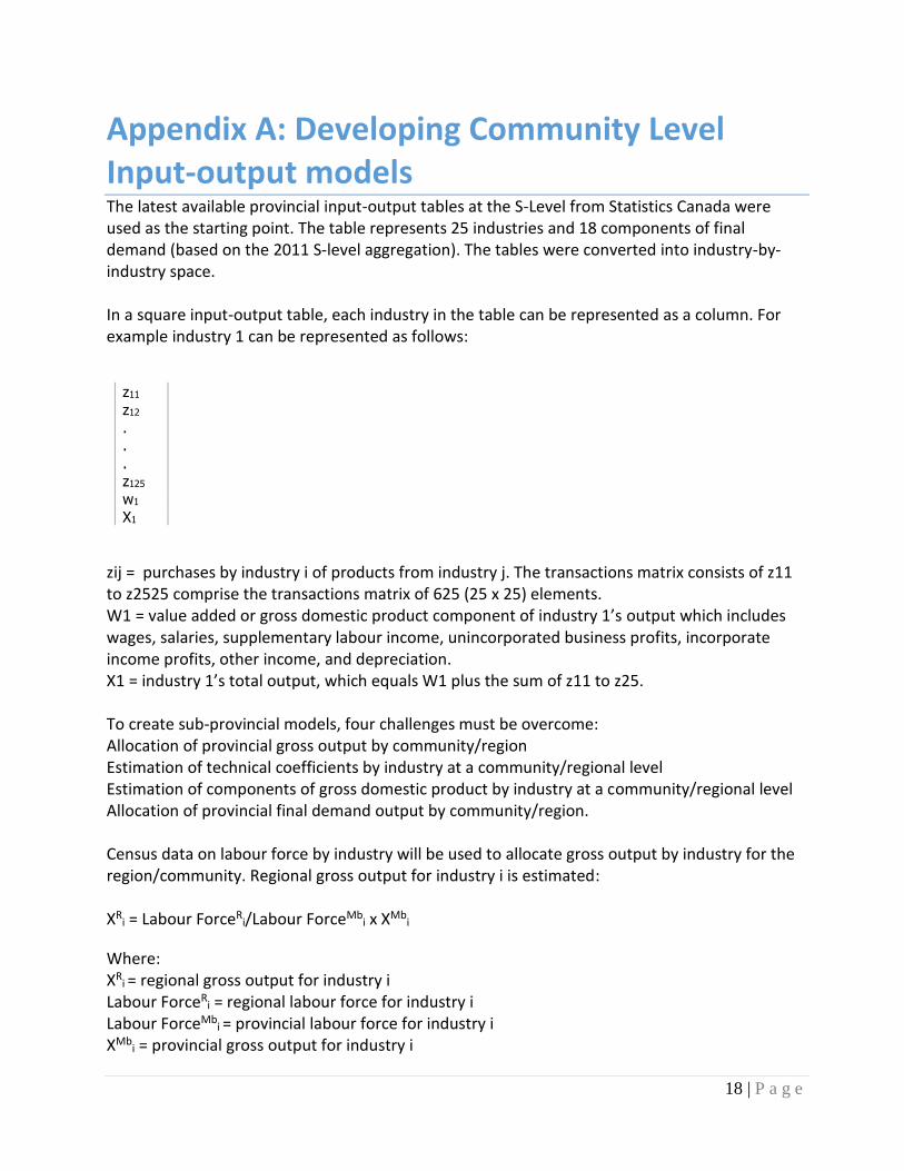
Appendix A: Developing Community Level Input-output models The latest available provincial input-output tables at the S-Level from Statistics Canada were used as the starting point. The table represents 25 industries and 18 components of final demand (based on the 2011 S-level aggregation). The tables were converted into industry-by-industry space. In a square input-output table, each industry in the table can be represented as a column. For example industry 1 can be represented as follows:

z11

z12

.

.

. z125

w1

X1

zij = purchases by industry i of products from industry j. The transactions matrix consists of z11 to z2525 comprise the transactions matrix of 625 (25 x 25) elements. W1 = value added or gross domestic product component of industry 1’s output which includes wages, salaries, supplementary labour income, unincorporated business profits, incorporate income profits, other income, and depreciation. X1 = industry 1’s total output, which equals W1 plus the sum of z11 to z25. To create sub-provincial models, four challenges must be overcome: Allocation of provincial gross output by community/region Estimation of technical coefficients by industry at a community/regional level Estimation of components of gross domestic product by industry at a community/regional level Allocation of provincial final demand output by community/region. Census data on labour force by industry will be used to allocate gross output by industry for the region/community. Regional gross output for industry i is estimated: XR

i = Labour ForceRi/Labour ForceMb

i x XMbi

Where: XR

i = regional gross output for industry i Labour ForceR

i = regional labour force for industry i

Labour ForceMbi = provincial labour force for industry i

XMbi = provincial gross output for industry i

19 | P a g e

To estimate items in each regional transaction matrix (zij) it will be assumed in all cases that the provincial input structure will apply to regional industries. The components of the regional transaction matrix are estimated:

zRij = zSK

ij/XMbi x XR

i Where: zR

ij = an element of the regional transactions matrix. zSK

ij = the corresponding element of the provincial transactions matrix. The same methodology is used for estimating the components of GDP. WR

i = WMbi/XMb

i x XRi

Where: WR

i = regional value added or gross domestic product component of industry i’s output WMb

i = provincial value added or gross domestic product component of industry i’s output The components of final demand are estimated as follows. Personal expenditures are based on a per capita allocation of provincial spending. PER

i = PEMbi/PopMb x PopR

Where: PER

i = Regional personal expenditure on industry i’s output PEMb

i = Provincial personal expenditure on industry i’s output PopMb = Provincial population PopR = Regional population Gross capital formation (GFCF) or investment by industry is estimated applying the regional share industry to total provincial gross capital formation for each industry. The same approach is used to estimate exports (Xd), imports (M), and inventory changes by industry (VPC) GFCFR

i = XRi/XMb

i x GFCFMbi

XdR

i = XRi/XMb

i x XdMbi

MRi = XR

i/XMbi x MMb

i VPCR

i = XRi/XMb

i x VPCMbi

Where: GFCFR

i = Regional investment spending on industry i’s output.

20 | P a g e

GFCFMbi = Provincial investment spending on industry i’s output

XdRi = Regional exports of industry i’s output

XdMbi = Provincial exports of industry i’s output

MRi = Regional imports of industry i’s output

MMbi = Provincial imports of industry i’s output

VPCRi = Regional inventory changes of industry i’s output

VPCMbi = Provincial inventory changes of industry i’s output

Regional public administration employment is used to allocate provincial government current expenditures by region. GCER

i = PAER/PAEMb x GCEMbi

Where: GCER

i = Regional government current expenditures on industry i’s output PAER = Regional public administration labour force PAEMb = Provincial public administration labour force

GCEMbi = Provincial government current expenditures on industry i’s output

It is also necessary to adjust for leakages for intra-provincial imported factors of production. These are estimated residually: If the sum of the use (both Final Demand and Inter-industry sales) of industry i’s output is less than Xi then, intra-provincial exports are used to balance. Similarly, if use is greater than Xi intra-provincial imports are used the balance. Intra-provincial exports/imports and exports due to out-shopping are estimated by calculating the marginal propensity to out-shop (the ratio of major community per capita retail sales to provincial per capita retail sales and multiplying by PE. Imports and exports are adjusted by this amount. The estimation of intra-provincial imports into a region/community and incorporation of intra-provincial imports into the region/community model’s leakages will constrain local multipliers to values not exceeding provincial level multipliers.

Developing Community/Regional Impact Models

Industry outputs in response to a shock in final demand are calculated as (I-(I-μ-α-β)A)-1((I-μ-α-β)e*+(I-μ-β)Xd+(I-μ)Xr)=X

Where:

I = an identity matrix of industry by industry dimension A = a matrix of technical coefficients representing inter-industry purchases (zij) divided by own industry gross output Xi. μ = a diagonal matrix whose elements represent the ratio of imports to use α = a diagonal matrix whose elements represent the ratio of government production to use β = a diagonal matrix whose elements represent the ratio of inventory withdrawals to use

21 | P a g e

e* = final demand categories of consumption, government purchases of goods and services, business and government investment, and inventory additions. Xd = final demand category of domestic exports Xr = final demand category of re-exports.

Employment is calculated as a fixed number of positions per dollar of industry output. GDP components are calculated based on a fixed ratio of Wi to industry output.

brandon growth forecast final report · brandon growth forecast final report ... total industrial...

Documents