Branching Avoidance in Kinematic Image Space

for Linkage Synthesis

Adam Nilsson, Lund University

11 mars 2013

Abstract

We consider a finite position synthesis and branching avoidance of four-bar link-ages based on kinematic theory derived from dual quaternions. The branchingdefect is defined as a situation where all specified task positions are not con-nected by a continuous motion of the linkage end effector. The workspace ofa four-bar linkage is derived to be the intersection of two hyperboloids in thekinematic image space. This is used to develop a fast method to determinebranching of a linkage and to find an explicit solution to the end effector tra-jectory. A new synthesis method is developed where one task position is givena lower priority. Using the new branching analysis method and by synthesizinglinkages with various values of one parameter of the linkage, we can determinea range of values for the constrained dimension which will give useful linkagesfor the four most prioritized task positions. Finally a method to find the closestuseful linkage to the last task position is derived.

Sammanfattning

Vi betraktar syntes och grendefekten av fyrlanks-mekanismer utifran ett bergan-sat antal task-positioner, baserat pa kinematisk teori harledd fran duala kvar-ternioner. Grendefekten ar definierad som situationen dar alla specificeradetask-positionerna inte ar sammankopplade av en kontinuerlig rorelse av me-kanismens end-effector. Arbetsomradet av en fyrlanks-mekanism ar harlett somsnittet mellan tva hyperboloider i det kinematiska bildrummet. Detta anvandsfor att utvackla en snabb metod for att avgora om grendefekten foreligger formekanismen, och for att harleda en explicit losning for mekanismens end effectortrajektoria. En ny syntes-metod ar utvacklad dar en av task-positionerna ar gi-ven en lagre prioritet. Genom att anvanda den nya grendefektsanalys-metodenoch berakna lank-mekanismer med varierande varden av mekanismens paramet-rar, kan vi hitta ett intervall av varden pa parametern som ger en anvandbarmekanism for de forsta fyra task-positionerna. Slutligen harleder vi en metodfor att avgora vilket varde pa parametern som ger den lank-mekanism som narnarmast den lagre prioriterade task-positionen.

1

Contents

1 Introduction 51.1 Linkage Mechanisms . . . . . . . . . . . . . . . . . . . . . . . . . 51.2 Synthesis of Four-Bar Linkages . . . . . . . . . . . . . . . . . . . 9

1.2.1 Homogeneous Transformation Matrices . . . . . . . . . . 101.3 Multiloop Linkages . . . . . . . . . . . . . . . . . . . . . . . . . . 10

1.3.1 Synthesis of a Watt Ia six-bar linkage . . . . . . . . . . . 111.4 Mechanism Branches . . . . . . . . . . . . . . . . . . . . . . . . . 121.5 Problem Statement . . . . . . . . . . . . . . . . . . . . . . . . . . 131.6 Outline and Approach . . . . . . . . . . . . . . . . . . . . . . . . 141.7 Related Work . . . . . . . . . . . . . . . . . . . . . . . . . . . . . 14

1.7.1 Kinematic Theory . . . . . . . . . . . . . . . . . . . . . . 141.7.2 Branching . . . . . . . . . . . . . . . . . . . . . . . . . . . 141.7.3 Branching Analysis in the Kinematic Image Space . . . . 15

2 Kinematics Theory 162.1 Quaternions and Dual Quaternions . . . . . . . . . . . . . . . . . 162.2 Kinematic Image Space . . . . . . . . . . . . . . . . . . . . . . . 17

2.2.1 Shapes in the Kinematic Image Space . . . . . . . . . . . 182.3 Constraint Manifolds . . . . . . . . . . . . . . . . . . . . . . . . . 18

2.3.1 Constraint Manifold for 2R Chain . . . . . . . . . . . . . 192.3.2 Obtaining the Constraint Manifold Equation . . . . . . . 20

2.4 Constraint Curve of a Four-Bar Linkage . . . . . . . . . . . . . . 242.5 Solving for the Constraint Curve . . . . . . . . . . . . . . . . . . 24

2.5.1 Arbitrary Hyperboloid Intersection . . . . . . . . . . . . . 27

3 Analysis of Branching in Kinematic Image Space 293.1 Determine Branches . . . . . . . . . . . . . . . . . . . . . . . . . 29

3.1.1 New Approach . . . . . . . . . . . . . . . . . . . . . . . . 293.1.2 Determine the Side of Infinite Curves . . . . . . . . . . . 333.1.3 The Side of a Closed Curve . . . . . . . . . . . . . . . . . 34

4 Modifying Task Positions 354.1 Intersection Shapes . . . . . . . . . . . . . . . . . . . . . . . . . . 354.2 Projection Methods . . . . . . . . . . . . . . . . . . . . . . . . . 35

2

4.2.1 Projecting on Curve given by an Implicit Equation . . . . 354.3 Discussion . . . . . . . . . . . . . . . . . . . . . . . . . . . . . . . 36

5 Four-Point Synthesis 375.1 Determine the Structure Intervals . . . . . . . . . . . . . . . . . . 375.2 Analyze the Branching Conditions . . . . . . . . . . . . . . . . . 385.3 Multiple Solutions . . . . . . . . . . . . . . . . . . . . . . . . . . 395.4 Example . . . . . . . . . . . . . . . . . . . . . . . . . . . . . . . . 405.5 Modifying the fifth task position . . . . . . . . . . . . . . . . . . 41

6 Discussions 436.1 Adjusting to Primitive Shapes . . . . . . . . . . . . . . . . . . . . 436.2 Structure interval . . . . . . . . . . . . . . . . . . . . . . . . . . . 436.3 Constraint Manifolds . . . . . . . . . . . . . . . . . . . . . . . . . 43

6.3.1 Order of Constraint Manifolds . . . . . . . . . . . . . . . 446.4 Synthesis of Non-Branching Six-Bar Linkages . . . . . . . . . . . 44

7 Conclusions 467.1 Kinematic Theory . . . . . . . . . . . . . . . . . . . . . . . . . . 46

7.1.1 Constraint Manifolds . . . . . . . . . . . . . . . . . . . . . 467.1.2 Constraint Curve of a Four Bar Linkage . . . . . . . . . . 46

7.2 Mechanism Branching . . . . . . . . . . . . . . . . . . . . . . . . 477.2.1 The Side of the Constraint Curve . . . . . . . . . . . . . . 48

7.3 Extruding all Possible Constraint Curves . . . . . . . . . . . . . . 487.4 Modifying a Fifth Task Position . . . . . . . . . . . . . . . . . . . 487.5 Future Work and Research . . . . . . . . . . . . . . . . . . . . . 48

A Dual Quaternions 49A.1 Quaternions . . . . . . . . . . . . . . . . . . . . . . . . . . . . . . 49

A.1.1 The Imaginary Dimensions . . . . . . . . . . . . . . . . . 49A.2 Dual Numbers . . . . . . . . . . . . . . . . . . . . . . . . . . . . 50A.3 Screw Displacement . . . . . . . . . . . . . . . . . . . . . . . . . 51A.4 Dual Quaternions . . . . . . . . . . . . . . . . . . . . . . . . . . . 52A.5 Notations . . . . . . . . . . . . . . . . . . . . . . . . . . . . . . . 53

3

Preface

Acknowledgments

The work behind this thesis was conducted at University of California Irvineduring the spring 2012. I specially want to thank my supervisor at UC Irvine,Michael McCarthy for giving me the opportunity of working with him, and forour valuable discussions during the work progress. I want to thank my LTHsupervisor Stefan Diehl and my lab partners at UC Irvine Mark Plecnik andKaustubh Sonawale for their support during the process. I also want to thankmy father Klas Nilsson and my sister Sofie Nilsson for many valuable commentson the report. Finally I like to thank the international offices at LU and LTHalong with the University of California Education Abroad program for givingme the opportunity to come to California and Irvine.

4

Chapter 1

Introduction

1.1 Linkage Mechanisms

Robots are getting more and more common in industrial environments and areprimary used to move objects between a set of positions. The object can beeither a tool or the product itself.

To ensure generality in the motion, the arm usually involves several degreesof freedom, so the same robot arm can be used for many different applications.A typical industrial robot has six motors and can move in six degrees of freedom,which is the full flexibility in a 3-dimensional space. A high degree of freedom isgood from a general perspective, but might be a disadvantage in other situation.

The automation industry today is generally more interested in robots withflexibility than designing a specific linkage which can only perform the taskit was designed for. However when a specific motion is known and no othermotion is of interest for the process, it might be much more convenient toconstrain the motion by designing a mechanism of less degrees of freedom, suchas a mechanical linkage.

Definition 1. A mechanical linkage is an assembly of bodies connected togetherto manage forces and movement.

There are both advantages in terms of performance and cost by using linkagemechanisms. A one degree of freedom linkage would require only one actuatorfor the same motion as a normal robot would require at least three actuatorsfor. Less actuators gives both lower cost and higher accuracy. Linkages can befound as components in many mechanisms and machines, some examples arethe following.

Example, Airplane Flaps Considering the flaps of an airplane wing. Flapsare used to change the aerodynamic property of the wing during start, land-ing and altitude changes. The optimal positions x, y and θ for the flaps aredetermined by aerodynamic calculations.

5

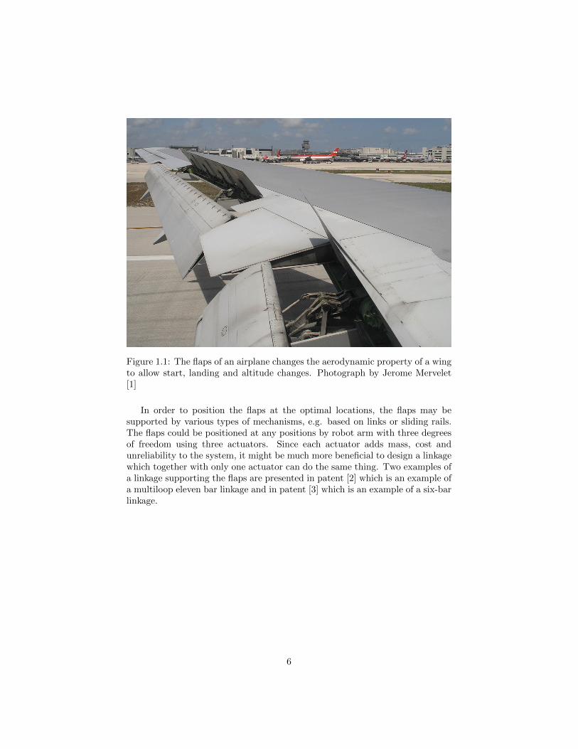
Figure 1.1: The flaps of an airplane changes the aerodynamic property of a wingto allow start, landing and altitude changes. Photograph by Jerome Mervelet[1]

In order to position the flaps at the optimal locations, the flaps may besupported by various types of mechanisms, e.g. based on links or sliding rails.The flaps could be positioned at any positions by robot arm with three degreesof freedom using three actuators. Since each actuator adds mass, cost andunreliability to the system, it might be much more beneficial to design a linkagewhich together with only one actuator can do the same thing. Two examples ofa linkage supporting the flaps are presented in patent [2] which is an example ofa multiloop eleven bar linkage and in patent [3] which is an example of a six-barlinkage.

6

Figure 1.2: This eleven-bar linkagemechanism was patented by Boeing in1981. It positions the flap at threespecified positions [2].

Figure 1.3: A six-bar linkage in aconfiguration named Stephenson III isused to control the motion of the flaps[3].

Example, Race Car Suspension The wheel of a car is required to movewhile the shocks deflects. Consider a car in straight motion seen from the front.In the view plane, a wheel has three degrees of freedom, x, y and rotation θ.

The wheel requires a supporting mechanism that allows the wheel to moveon a one-dimensional trajectory, which is finally controlled by the shocks. Ifa robot arm with three degrees of freedom was used to support the wheel, itwould require at least two actuators together with the shock to constrain thewheel motion. Since there are huge forces involved in a car suspension, themotors would have to produce a lot of force even though the actual work wouldbe minimal. It is much more beneficial to design a support mechanism withonly one degree of freedom and let the shock control the final motion.

A double wishbone car suspension, see Figure 1.4, commonly refereed to asdouble A-arm, is an example of a four-bar linkage when seen in the front plane.The car chassis is considered as one link, the two wishbones or A-arms are onelink each and the upright is the fourth link. This mechanism can be found inmost competitive race-cars.

This master thesis will primary consider four-bar linkages, which is the mostbasic linkage mechanism. It is still of interest to study since more complexlinkages can be synthesized as a combination of open chains and four-bar linkages[6].

Example, Trunk Closing Mechanism A design example for a linkage isto move an object along a path or through a set of positions. An example of apossible design case is the trunk cover in an automotive.

7

Figure 1.4: A double wishbone suspension is used in many competitive race-carssuch as this Formula Student [4] car LUR5 from LU Racing [5].

Figure 1.5: Chrysler Sebring 2005 has a four-bar linkage to support the trunkcover motion.

Figure 1.5 shows the trunk linkage in a Chrysler Sebring. The design criteriain this example is that the trunk should be positioned in a closed and an openedposition. Two intermediate positions could also be specified near the openedand the closed position to obtain a smooth closing motion, the lock mechanismmay need to be hooked in from a certain direction while closing.

The alternative to a linkage in this case is a much longer curved bar con-nected to a hinge inside the trunk, which is the most common design in coupe

8

cars.

1.2 Synthesis of Four-Bar Linkages

A four-bar consists of a ground link, two crank links and a coupler link. In thecase where the linkage is driven by one of the cranks, the other crank is calledthe follower.

gx

gy

py

px

l

Wi

Figure 1.6: Drawing of a four-bar linkage with dimension-annotations for one ofthe cranks. The two blue lines are called the crank links and the orange triangleis called the coupler link. The fourth link is the ground.

Linkage synthesis is the process of generating a linkage that satisfies somedesign specifications. In this thesis we will consider synthesis where the dimen-sions of the linkage is calculated so the end effector can be positioned at a setof task positions.

Definition 2. A position consist of a translation and a corresponding rotation.A task position is a position used to define the task for a mechanism.

A crank of a four-bar linkage is defined by its ground pivot, link lengthand position of the moving pivot relative to the end effector frame. Usinghomogeneous transformation matrices, the vector along a crank link can bewritten as:

−→l = Wi

pxpy1

− gx

gy1

(1.1)

9

where Wi is the matrix describing task position number i. The length of thelink is then given by:

l2i =

Wi

pxpy1

− gx

gy1

T Wi

pxpy1

− gx

gy1

(1.2)

The equation has either zero, two or four real solutions (px, py, gx, gy, li) [7].At least two solutions are necessary since we need two different cranks.

1.2.1 Homogeneous Transformation Matrices

For the unoriented reader a quick review of homogeneous transformation ma-trices is given. If coordinate system W is located with origin in the point ~p andthe coordinate axes are given by the vectors ~ex and ~ey, then the homogeneoustransformation matrix is given by:

W =

(~ex ~ey ~p0 0 1

)(1.3)

A vector ~v = (x, y, 1)T in W or a vector ~v = (x, y, 0)T in a coordinate systemwith the same rotation as W and origin at the parent’s origin is given in theparent coordinate system by:

~v0 = W~v (1.4)

In other terms, the zero as the last element means that the vector should beconsidered from an origin while the number one means that the vector shouldbe translated to an origin of an other coordinate system. Several frames canbe added in a chain by matrix multiplication. The last element in the vectoris useful since the coordinate axes will always start in the origo of the lastcoordinate system but will be rotated by all parent coordinate systems.

1.3 Multiloop Linkages

The four-bar linkage consists of only one kinematic loop. More complex linkagescan be constructed using more kinematic loops. A six-bar linkage consists ofsix links connected by seven joints and can be arranged in several differentways. McCharty presents a method for synthesizing six-bar linkages in [6], seeFigure 1.8. The method is to first specify a 3R chain, which has three degreesof freedom and can reach any position within its work space. The 3R chain isconstrained by adding more links. Those extra links can by synthesized withthe four-bar synthesis methods. Patent [3] is an example of an application ofwhere six-bar linkage is composed from four-bar linkages. The inventor writeexplicitly in the abstract that it is a six bar linkage built with a four bar linkageas a component.

10

Stephenson I

Stephenson IIa

Watt Ia

Watt Ib

Step 2

Step 1

0 1 2 3

0 1 2 3

0 1 2 3

0 1 2 3

4

4

4

4

Figure 1.7: The different arrangement of links for a six-bar linkages. From a 3Rchain, the red link is synthesized first using the same method as for four-bars.[6]

1.3.1 Synthesis of a Watt Ia six-bar linkage

To synthesis a six-bar Watt Ia linkage, one start with a 3R chain reaching alltask positions. Since a 3R chain has 3 degrees of freedom it can reach anypositions as long as they are within a certain distance. E.g. if all the links havethe length l = 1, a position that are further away than three from the base is ofcourse not possible to reach. A similar case occurs for example if the first linkhas length l1 = 10 and the second and third has the lengths l2 = l3 = 1, then aposition closer than eight from the base is of course never reachable.

11

F1

F2

F0

F3

1

5

4

3

2

Figure 1.8: A Watt Ia six-bar linkage drawing from [6] with notations added on.

In order to constrain the 3R chain, first the position of frame F2 in frameF0 is calculated at all task positions. Then a four-bar can be synthesized withlink 1 and link 4 as the cranks and link 2 as the coupler.

A frame F3 is fixed to link 4 and the position of frame F1 given in frameF3 is calculated at all task positions. A four-bar with link 4 as the ground canthen be synthesized. Link 2 will be one of the cranks which is already definedat this time. Link 5 will be the second crank in this four-bar.

1.4 Mechanism Branches

Some linkages can be assembled in different configurations, and will dependingon the configuration follow different trajectories. Different terminology mayexist in different literature. Depending of design requirements the usefulnessof a linkage may be different. To avoid confusions or misunderstandings, somedefinitions are introduced.

12

Figure 1.9: Drawing of a branching four-bar linkage in two different configura-tions. The reachable trajectory is different for the two configurations.

Definition 3. A configuration of a linkage and its continuous motion is calleda branch of the linkage. When the task positions lie in different branches,the linkage is branching and not useful.

Definition 4. A linkage with all task positions in the same branch is called auseful linkage.

The existence of a solution to (1.2) only tells that the linkage can be assem-bled at each of the task position in some configurations, but there does not haveto be a continuous motion between the task positions. I.e. the task positionsmay belong to different branches of the mechanism. It does not have to be anissue when the linkage has two branches as long as all task positions lie in thesame branch.

1.5 Problem Statement

It is not yet well known what causes the mechanism to branch. The currentapproach to find non-branching linkages is to define a tolerance zone for the taskpositions and randomly choose task positions in the zone until a non branchinglinkage is found. This process is much time consuming and will give differentresults each time. This thesis will investigate the conditions for what causesthe mechanism to branch and to find a strategy of modifying task positions togenerate the best possible non-branching linkage.

13

1.6 Outline and Approach

• First some kinematic theory that is necessary for the later work will beintroduced, and some equations describing the kinematics of 2R chainsand four-bar linkages are derived. The equations are referred to as theconstraint manifold equations.

• The conditions of when a mechanism branches are analyzed in detail inorder to find a fast method to analyze the branching structure of a four-barlinkage.

• The shape of the constraint curve (which is a curve describing the motionof a mechanism) is analyzed and a first approach to find useful linkageswill be to project the task positions onto curves with shapes similar toshapes that a single branch constraint curve may take. The first approachdid not increase the number of useful linkages, so a second approach wasconsidered.

• The second approach to find useful linkages will be to only consider fourtask positions at a beginning. Then all possible linkages to those fourtask positions will be calculated. Using the branching analysis method,all useful linkages to the four task positions will be calculated and a fifthtask position will be projected on to the motion of the closest matchinglinkage.

1.7 Related Work

1.7.1 Kinematic Theory

Linkage synthesis is not a prioritized field and the research is progressing ratherslowly. The approach in this thesis is based on the theory of quaternions ex-plored in 1844 by Hamilton [8] and geometry in the kinematic image spacepresented in 1911 by Grunwald [9]. Not much has been done based on thistheory. Bottema and Roth have a rigorous introduction to the theoretical kine-matics [10] including dual quaternions and constraint manifold. McCarthy [7]gives an easier introduction to the theoretical kinematics.

1.7.2 Branching

Branching and usefulness of linkages have been approached in different ways.I have defined a linkage as useful if there is a continuous motion between thetask positions, and it is assumed that the mechanism can be actuated along thedesired motion. Chase [11] and Parrish [12] considered linkages that are drivenby rotation of one crank, which introduces singularity configurations where thedriving link can not control if the linkage will move in one or another direction.Chase defines a branch as the range of motion which can be uniquely controlledby a rotating input link. What is defined as a branch in this thesis is called a

14

Circuit by Chase. By writing the kinematic loops for the linkage and analyze theJacobian of the loop equations at each task position, Parrish [12] can disqualifysome linkages immediately, but to classify them as useful he needs to do a closernumeric analysis of the motion.

1.7.3 Branching Analysis in the Kinematic Image Space

The closest related work to this thesis is presented by Schrocker in 2005[13]and 2007[14]. Schrocker uses constraint manifold equations of 2R chains. Thebranching conditions are determined by the intersection between two constraintmanifolds. Schrocker derives the same property of the constraint manifoldshapes as is done in this thesis. However Schrocker’s derivations are different.The results in [13] and [14] appear to be the same as in Chapter 3.

15

Chapter 2

Kinematics Theory

The kinematics of an arbitrary linkage is in the general case non-linear. Thiscauses problems for design, analysis and control of such mechanism. An ar-bitrary non linear algebraic equation has usually no exact explicit solution.However in some special cases when a variable transformation exist, it might bepossible to obtain an exact solution.

2.1 Quaternions and Dual Quaternions

In 1844, William Rowan Hamilton[8] explored a mathematical object which henamed quaternions. The quaternions was an extension of the complex numbersfrom one imaginary dimension i into three imaginary dimensions i, j and k.They have shown to be very useful to represent rotations and are used in manyrobotics and flight control systems today.

Theory of dual numbers where later on used to extend the quaternions todual quaternions, which can be used to represent a displacement with bothrotation and translation. A dual quaternion consist of two quaternions, one realand one dual part, which gives a total of eight elements. The real part is onlyrelated to the rotation while the dual part is related to a combination of therotation and translation.

A more common way of representing translations and rotations today is byusing vectors and rotation matrices. The quaternions where Vectors where theinspiration for J.W. Gibbs when invented the vectors in 1884 [15].

The reader is referred to Appendix A for an introduction to dual quaternions.In the case of planar kinematics, only four non-zero elements remain of the dualquaternion.

Definition 5. A planar dual quaternion is the four components of a dual quater-nion which are non-zero for a planar displacement.

A planar displacement (x, y, θ) can be expressed with a planar dual quater-

16

nion given by:

Q = (q1, q2, q3, q4) ==(cos(θ2

), sin

(θ2

), x2 cos

(θ2

)+ y

2 sin(θ2

), y2 cos

(θ2

)− x

2 sin(θ2

)) (2.1)

Because of the trigonometric unity, any planar dual quaternion has to satisfythe condition q21 + q22 = 1.

Definition 6. A planar dual quaternion that satisfies the unity condition

q21 + q22 = 1 (2.2)

is called a displacement planar dual quaternion.

The unity condition can easily be enforced by the operator

Pd(Q) =Q√

Q21 +Q2

2

(2.3)

Pd is a projection operator (which means if the operator Pd is applied to aobject in the range of Pd, the same object is returned), operating from the four-dimensional domain of all planar dual quaternions into the projection space ofall displacement planar dual quaternions.

2.2 Kinematic Image Space

To simplify visualization of a planar dual quaternion, it is useful to project itonto a three-dimensional space. It will show to be convenient to use the spacedefined by:

Definition 7. The projection space S of the operator:

PS(Q) =

(q1q1,q2q1,q3q1,q4q1

)= (1, s1, s2, s3) (2.4)

is called the kinematic image space, and was first introduced by [9].

Definition 8. The pointS = (s1, s2, s3) (2.5)

is called the image point of the displacement defined by the planar dual quater-nion Q.

Theorem 1. The image point of a displacement x, y and rotation θ is given by:

S = PS(Q) =

[tan

(θ

2

),

1

2

(x+ y tan

(θ

2

)),

1

2

(y − x tan

(θ

2

))]=

=

[s1,

1

2(x+ ys1),

1

2(y − xs1)

](2.6)

17

Proof. The planar dual quaternion of a displacement is given by (2.1) to be:

Q =

(cos

(θ

2

), sin

(θ

2

),x

2cos

(θ

2

)+y

2sin

(θ

2

),y

2cos

(θ

2

)− x

2sin

(θ

2

))(2.7)

The image point is obtained by applying the projection operator (2.4)

Q

q1=

[1, tan

(θ

2

),

1

2

(x+ y tan

(θ

2

)),

1

2

(y − x tan

(θ

2

))](2.8)

The image point is given by the last three components.

As one can see, the first component is only related to the rotation, while thetwo last components are a combination of translation and rotation.

2.2.1 Shapes in the Kinematic Image Space

The map between the physical dimensions to the image space is non linear.Some non-linear kinematics in the spatial dimensions takes a nice form afterthe non linear mapping. A straight line in S can describe a curved motion inthe spatial dimensions.

Rotate around a point in the spatial dimension

It can be observed in (2.6) that a rotation around a point in the physical di-mension is described by a line in the kinematic image space.

Translate without rotating

From (2.6), it can also observed that a translation along a straight line withoutrotation will follow a straight line with a constant x-value, x = s1.

2.3 Constraint Manifolds

A constraint manifold is the set of positions the end effector of a mechanismcan reach. For a 2R chain (Figure 2.1) which has two degrees of freedom, theconstraint manifold forms a surface. For a one degree of freedom linkage, like afour-bar linkage, the constraint manifold is a curve, called the constraint curve.The constraint manifolds for 2R chains are importance when studying four-barlinkages since the four-bar can be seen as two 2R chains with the coupler linkas a common second link. The constraint curve is then the set of points reachedby both 2R chains, and therefore the intersection of two 2R chains’ constraintmanifolds.

18

Φ-

Θ

a

End Effector Frame

Coupler Link

(Second Link)

Crank

(First Link)

Figure 2.1: A 2R chain consists of two links. The first link is connected to theground by a rotation joint. The second link is connected to the first with asecond rotation joint. The end effector can be located anywhere on the secondlink.

2.3.1 Constraint Manifold for 2R Chain

The constraint manifold equation of a 2R chain will be derived by writing thekinematics with planar dual quaternions. This gives four equations, one for eachcomponent in the planar dual quaternion. The kinematic variables (the jointangles) is eliminated from the equations and the constraint manifold equationis obtained.

Forward Kinematics for 2R chain

Let T (x, y) be a dual quaternion describing a pure translation, R(θ) be a dualquaternion describing a pure rotation. The dual quaternion Q of the end effectoron the second link is obtained by dual quaternion multiplications, denoted by⊗.

Q = T (gx, gy)⊗R(θ)⊗ T (a, 0)⊗R(φ)⊗ T (px, py) (2.9)

This can be expanded into:

Q =

cos(θ+φ2

)sin(θ+φ2

)12

(a cos

(θ−φ2

)+ (gx + px) cos

(θ+φ2

)− py sin

(θ+φ2

))12

(a sin

(θ−φ2

)+ (px − gx) sin

(θ+φ2

)+ py cos

(θ+φ2

))

(2.10)

19

2.3.2 Obtaining the Constraint Manifold Equation

It is desirable to find a constraint manifold equation that works both for alldisplacement planar dual quaternions and in the kinematic image space.

Theorem 2. If the constraint manifold equation is a homogeneous equationwith all terms of the same order (e.g. q2i or qiqj if the order is two), and thedual quaternion Q satisfies the constraint manifold equation, then all multiplesof Q (i.e. tQ for t ∈ R) satisfies the constraint manifold equation.

Proof. The proof is given for second order terms. This is the only order thatwill be used later on, but it is easy to make the proof for any other order aswell. Let Q = (q1, q2, q3, q4)T . The constraint manifold equation can be writtenas the sum of all possible combinations of qi and qj .

K(q1, q2, q3, q4) =

4,4∑i=1,j=1

ci,jqiqj = 0 (2.11)

Let P = tQ, such that pi = tqi. Then

4,4∑i=1,j=1

ci,jpipj =

4,4∑i=1,j=1

ci,jt2qiqj = t2

4,4∑i=1,j=1

ci,jqiqj ⇐⇒ (2.12)

4,4∑i=1,j=1

ci,jpipj = t2 · 0 = 0 (2.13)

This proves that if the constraint manifold equation is satisfied for a planar dualquaternion Q, it is also satisfied by a planar dual quaternion P = tQ.

There is a linear map between the four trigonometric functions cos( θ+φ2 ),

sin( θ+φ2 ),cos( θ−φ2 ) and sin( θ−φ2 ) and the components of the planar dual quater-nion q1, q2, q3 and q4, since (2.10) can be written as:

q1q2q3q4

=

A

4×4

cos( θ+φ2 )

sin( θ+φ2 )

cos( θ−φ2 )

sin( θ−φ2 )

(2.14)

The variables θ and φ can be eliminated in (2.10) by first extracting thevalues of the trigonometric functions in terms of qi, then square and use thetrigonometric unity.

20

Let:

c1 = cos(θ + φ

2) (2.15)

c2 = sin(θ + φ

2) (2.16)

c3 = cos(θ − φ

2) (2.17)

c4 = sin(θ − φ

2) (2.18)

According to the trigonometric unity cos2(x) + sin2(x) = 1:

c21 + c22 − c23 − c24 = 1− 1 = 0 (2.19)

By substituting ci with its values in terms of the components in the dual quater-nion (C = A−1Q), the constraint manifold equation is obtained as:

K(q1, q2, q3, q4) = q21 + q22 −1

a2[(gxq1 + gyq2 − pxq1 + pyq2 − 2q3)2+

(gxq2 − gyq1 + pxq2 + pyq1 + 2q4)2]

= 0 (2.20)

Interpreting the Constraint Manifold Equation

It is easy to see that the constraint manifold equation is a second degree poly-nomial equation of the four variables qi. However more structures are hiddenin the equation.

By writing (2.20) as a quadratic form

QTMQ = 0 (2.21)

with the symmetric matrix M given by:

21

M1,1 = −2(gx − px)2

a2− 2(py − gy)2

a2+ 2

M1,2 = −2(gx + px)(py − gy)

a2− 2(gx − px)(gy + py)

a2

M1,3 =4(gx − px)

a2

M1,4 = −4(py − gy)

a2

M2,2 = −2(gx + px)2

a2− 2(gy + py)2

a2+ 2

M2,3 =4(gy + py)

a2

M2,4 = −4(gx + px)

a2

M3,3 = M4,4 = − 8

a2

M3,4 = 0

(2.22)

It can easily be seen that (2.22) contains 8 different elements or coefficients.The symmetry of M reduces it to 10 of maximum 16 possible coefficients. Onecoefficient is zero and two of them are equal, which reduces it to 8. Sincethe equation is homogeneous, there is an infinite number of solutions for thecoefficients. By assigning one of the coefficients a value, the number of solutionsis reduced to one. Since (2.20) is a homogeneous equation, it is according toTheorem 2 valid for all scale’s of planar dual quaternions. To simplify geometricreasoning, the constraint manifold will from now on be analyzed in the kinematicimage space S, which gives three dimensions instead of four.

Consider a quadratic form in S of the same structure with the elements ci.The constraint manifold equation in the kinematic image space is given by:

(1 x y z

)m1 m2 m3 m4

m2 m5 m6 m7

m3 m6 m8 0m4 m7 0 m8

1xyz

= 0 (2.23)

The zeros tell that there is no product between y an z. The coefficient forboth y2 and z2 is c8, which generates a circle for a constant value of x. Bychoosing m8 = 1 we can expand and rewrite (2.23) as:

(y − (m6x+m3))2 + (z − (m7x+m4))2 − (m5 +m6 +m7)x2−2(m2 +m3m6 +m4m7)x− (m1 +m2

3 +m24) = 0 (2.24)

Even though we have seven different coefficients, they are all determined bythe five independent linkage parameters. By matching the values of m1 with

22

the corresponding elements in (2.22), one can observe that:

m5 +m6 +m7 = m1 +m23 +m2

4 =(a

2

)2(2.25)

andm2 +m3m6 +m4m7 = 0 (2.26)

Which simplifies (2.24) into:

(y − (m6x+m3))2 + (z − (m7x+m4))2 =(a

2

)2(1 + x2) (2.27)

This shows that the constraint manifold is a hyperboloid centered in

(0,m3,m4)

and with a center line direction

(1,m6,m7)

The radius of the circle at a fixed x is

r(x) =a

2

√1 + x2

Figure 2.2: A constraint manifold of a 2R chain takes the form of a hyperboloidcentered at the point (0,m3,m4) and with a centerline direction of (1,m6,m7)

By matching the values in (2.23) and (2.22), the center line and radius ofthe hyperboloid is found to be:

center(x) =1

2(2x, gx − px + x(gy + py), gy − py − x(gx + px)) (2.28)

radius(x) =a

2

√1 + x2 (2.29)

23

Coupler Link

Crank

Second Crank

End Effector Frame

Figure 2.3: A four bar linkage is constructed by two 2R chains with a commoncoupler link.

2.4 Constraint Curve of a Four-Bar Linkage

Consider a four-bar linkage constructed by a pair of 2R chains, with a com-mon coupler link. Also consider the two constraint manifold equations for the2R chains. For simplicity, one of the equations is for now assumed to take asimplified shape.

y − (m6x+m3))2 + (z − (m7x+m4))2 =(a

2

)2(1 + x2) (2.30)

y2 + z2 =(r

2

)(1 + x2) (2.31)

The end effector of the four bar has to satisfy both constraint manifold equa-tions, and is therefore given by the intersection curve.

2.5 Solving for the Constraint Curve

It is possible to find an explicit solution of the constraint curve. Consider twocircles with radius R and r with a distance d from each other along the firstcoordinate axis. The two intersection points, see Figure 2.4, are given by:(

d2 − r2 +R2

2d,±√−d4 + 2d2r2 + 2d2R2 − r4 + 2r2R2 −R4

2d

)(2.32)

24

R r

d

Figure 2.4: Two circles with radius R and r with their centers at distance dfrom each other. The intersection between the circles is given by (2.32).

Consider two constraint manifold hyperboloids at a fixed x-value. This givestwo circles. Align a coordinate system L with origo on the first center line andthe y-axis (Green in Figure 2.5) pointing in the direction of the second centerline. The first hyperboloid is for now assumed to have the trivial shape. Thez-axis (Blue) is chosen to be in the same x = constant plane and orthogonal tothe y-axis.

25

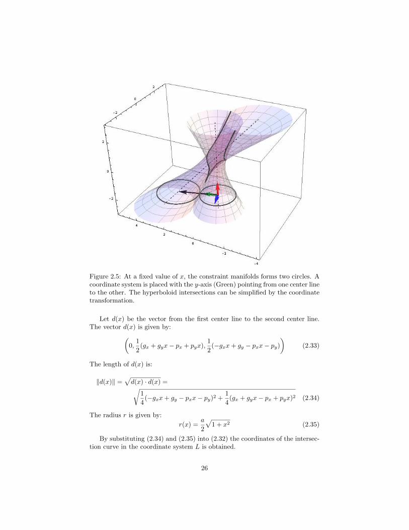
Figure 2.5: At a fixed value of x, the constraint manifolds forms two circles. Acoordinate system is placed with the y-axis (Green) pointing from one center lineto the other. The hyperboloid intersections can be simplified by the coordinatetransformation.

Let d(x) be the vector from the first center line to the second center line.The vector d(x) is given by:(

0,1

2(gx + gyx− px + pyx),

1

2(−gxx+ gy − pxx− py)

)(2.33)

The length of d(x) is:

‖d(x)‖ =√d(x) · d(x) =√

1

4(−gxx+ gy − pxx− py)2 +

1

4(gx + gyx− px + pyx)2 (2.34)

The radius r is given by:

r(x) =a

2

√1 + x2 (2.35)

By substituting (2.34) and (2.35) into (2.32) the coordinates of the intersec-tion curve in the coordinate system L is obtained.

26

Transform Coordinates

The coordinate transformation from L to an initial coordinate system is de-scribed by the matrix L(x)

L(x) =1

‖d(x)‖

‖d(x)‖00

0dy(x)dz(x)

0−dz(x)dy(x)

(2.36)

Since the x-axis remains the same, the y-axis is given by the vector d(x) andthe z-axis is the vector d(x) rotated a quarter revolution.

By substituting the values of R, r and d into (2.32), one obtain the intersec-tion in the coordinate system L:

CL(x) =

s1s2s3

(2.37)

Where:s1 = x (2.38)

s2 =a2(−(x2 + 1

))+ (x(gx + px)− gy + py)2 + (gx + x(gy + py)− px)2 + x2 + 1

4√

(x(gx + px)− gy + py)2 + (gx + x(gy + py)− px)2

(2.39)

s3 = ±√a4(− (x2 + 1)

2)

+ 2a2 (x2 + 1) ·

· ((x(gx + px)− gy + py)2 + (gx + x(gy + py)− px)2 + x2 + 1)−

− ((x(gx + px)− gy + py)2 + (gx + x(gy + py)− px)2 − x2 − 1)2/

4√g2x (x2 + 1) + 2gx (px (x2 − 1) + 2pyx) + g2y (x2 + 1)−

2gy (2pxx− pyx2 + py) + (x2 + 1)(p2x + p2y

)(2.40)

The constraint curve in a original coordinate system is finally obtained by thematrix multiplication:

C(x) = L(x)CL(x) (2.41)

2.5.1 Arbitrary Hyperboloid Intersection

In the case of two arbitrary constraint manifolds, the coordinate transformationgets a bit more complex. The vector between the center lines is obtained in thesame way but will now include more coefficients. The new x-axis will take thedirection of the first center line. A basis vector for the x-axis can for examplebe obtained by:

ex = center1(1)− center1(0) (2.42)

27

The new coordinate system is translated from (x, y, z) = (x, 0, 0) into theposition given by the first center line. The vector between the center lines isobtained by:

d(x) = center2(x)− center1(x) (2.43)

The ey vector is obtained by normalizing the vector d(x)

ey(x) =center2(x)− center1(x)

‖center2(x)− center1(x)‖(2.44)

The ez vector can be obtained by rotating ey by the angle π/2.

ez(x) = R{x,π2 } · ey(x) (2.45)

The constraint curve is then given by:

C(x) = center1(x) + [ex, ey(x), ez(x)]CL(x) (2.46)

There is no real reason for writing out the expression for the constraint curvesince it will cover more than a page. However we have shown that an explicitsolution does exist.

28

Chapter 3

Analysis of Branching inKinematic Image Space

In the case of real solutions of the constraint equations, there is a linkage thatgoes through all the task positions. However the different task positions maybelong to different branches of the linkage.

3.1 Determine Branches

A today’s approach to analyze branching of linkages is to form the equations ofa closed kinematic loop and solve the end effector position for a discrete set ofvalues for one of the links angles.

3.1.1 New Approach

With our new explored knowledge, the branching analysis can be done in a muchfaster way. By solving for the x-values were the constraint manifolds intersectsin only one point, a set of intervals, which are candidates to include continuousconstraint curves, is obtained. By just checking one point inside each intervalwe will know wherever there is a continuous curve inside the whole interval ornot. The task positions must all lie in the same interval for the linkage to beuseful.

The structure of the constraint curve was investigated by Schrocker et al. in[14]. They state that the constraint curve has two affinely finite branches, onebranch or two affinely infinite branches. This is not the whole truth about theconstraint curve. The constraint curve can take one of the five forms shown inFigure 3.1.

Consider a fixed value of x. As shown previously, each manifold forms acircle for a fixed value of x. The circles intersects in either zero, one, two orall points. Intersection in all points only occurs when both the center lines

29

(a) One closed affinely finite constraintcurve.

(b) Two half open infinite constraintcurves.

(c) One closed affinely finite, and two halfopen infinite constraint curves.

(d) Two closed affinely finite constraintcurves.

(e) Two infinite constraint curves.

Figure 3.1: Illustration of the possible structures of the constraint curve.

30

intersects and the two radius are equal at the same time, which is the case foran ideal parallel linkage (Figure 3.2). This case is not of big interest for us.

Figure 3.2: An ideal parallel linkage. The end effector orientation remainsconstant while the position moves on a circle.

Two circles intersect at one point if the distance between the center lines isthe same as either the difference in radius or the sum of radius. Those conditionscan be formulated as

‖∆r(x)‖ = ‖center2(x)− center1(x)‖ (3.1)

‖Σr(x)‖ = ‖center2(x)− center1(x)‖ (3.2)

Two intersection points occur when the distance between the center lines isin between the sum and the difference of radius.

‖∆r(x)‖ < ‖center2(x)− center1(x)‖ < ‖Σr(x)‖ (3.3)

The absolute values can be eliminated by squaring the equations.

∆r(x)2 = (center2(x)− center1(x)) · (center2(x)− center1(x)) (3.4)

Σr(x)2 = (center2(x)− center1(x)) · (center2(x)− center1(x)) (3.5)

Those equations are second degree polynomials since the center lines are givenby first degree polynomials, and the radius are square roots of a second degreepolynomial.

31

Note It is important to mention that the product of two square roots doesnot form a polynomial of the same order as the square root’s arguments in ageneral case. However it does in this case since the square roots have the samearguments.

It is of interest to study for which x values one solution occurs. Since theequations are quadratic, they can have zero, one or two distinct real solutions.Since there are two equations, there can be a maximum of four x values wherethe constraint manifolds intersects in only one point. Those points will bereferred to as the split points since they splits the image space into intervalsIs that either includes no intersection points or includes two intersection pointsfor each x-value. This means that for an interval Is, there is either a continuousconstraint curve covering the whole interval or no constraint curve at all, exceptat the boundary which is shared with the neighbor intervals.

The four split points xi form four intervals for possible constraint curves.The first instinct would suggest either three or five intervals, which are:

]−∞, x1], [x1, x2], [x2, x3], [x4, x5], [x5,∞[

or[x1, x2], [x2, x3], [x4, x5]

but certain attention has to be considered at infinity.

The case x→∞

The first dimension in S is represented by x = tan(θ2

). This means that x →

±∞ corresponds to the angle θ → ±π. It was shown in section 2.2.1 that a lineof the form [

s1,1

2(y + zs1),

1

2(z − ys1)

](3.6)

describes all position with the translation (y, z) in the physical dimensions.The ends at infinity of such a line will connect to each other in the physicaldimensions, since the angle θ = −π gives the same position as θ = π.

A linkage that includes θ = π in its work space will have a constraint curvethat goes to infinity and connects to an other curve at minus infinity. Therewill be a line of form (3.6) tangent to the constraint curves on the ends that areconnected together.

The reason for four intervals is that ±∞ are connected together and thereforethe last and first value forms one interval. The four intervals are:

[x1, x2] (3.7)

[x2, x3] (3.8)

[x3, x4] (3.9)

[x4, x1] (3.10)

32

Figure 3.3: The image space is divided into a maximum of four regions whicheither contains a constraint curve for all x or no constraint curve at all.

Physical Interpretation

The physical interpretation of this is that a linkage movement can be limited bya maximum angle and a minimum angle. At the maximum and minimum anglethere is only one translation the end effector can take. For any angle in betweenthere are two different translations. It also means that a four-bar linkage cannot have more than two translations with the same orientation.

3.1.2 Determine the Side of Infinite Curves

In the case of two infinite constraint curves there are no split points whichimplies that all task positions lie in the same interval. However it also impliesthat there are two decoupled constraint curves since they never join each otherin a single point. To determine which one of the curves an image point belongsto, the image point can be transformed to the coordinate system L. The signof the z-component will then determine which one of the curves an image pointbelongs to.

33

Figure 3.4: Two infinite constraint curve. By analyzing an image point in thecoodinate system L(x), the sign of the z-component (Blue axis) will determinewhich one of the curves the point belongs to.

3.1.3 The Side of a Closed Curve

Chase[11] considers a linkage useful if it can be driven by rotating one input linkand still reach all task positions. At some values of the input angle a linkagereaches a maximum or minimum value of the end effector rotation. There aretwo different trajectories leading to this position and it may not be possible tocontrol which one of the trajectories the end effector will follow when leavingthe position. Since the end effector rotation is directly related to the x-valuein the kinematic image space, the minimum and maximum values of the endeffector trajectory will occur at the split points.

Chase[11] defines a linkage as useful if all task positions can be reachedwhen the linkage is actuated by rotation of one of the links. Therefore it is ofinterest to determine which side of a closed curve an image point belongs to. Todetermine the side, the same method as in Section 3.1.2 can be applied. Evenif the usefulness defined by Chase[11] is not primary considered in this theses,the method is still able to use Chase’s definition.

34

Chapter 4

Modifying Task Positions

The first approach to avoiding branching was to identify some primitive approx-imate shapes for the constraint curve and adjust the task positions to mach oneof those primitive shapes.

4.1 Intersection Shapes

By experimenting with moving two cylinders it is observed that the shape ofthe intersection goes from one ellipse to a guitar shape, a figure eight and twoellipses. Those shapes are just approximations and hyperboloids may form muchmore complex intersections. It is still reasonable to think that five task positionsthat lie close to one of those shapes should have a non branching linkage.

This is investigated by matching an ellipse (which is the most simple case)to four of the task positions and projecting the fifth position onto the ellipse.

An general ellipse is determined by five coefficients. When the ellipse ismatched to four points, there is an infinite number of solutions. In the experi-ments, the ellipse closest to a circular shape where selected.

4.2 Projection Methods

4.2.1 Projecting on Curve given by an Implicit Equation

Consider a curve C defined by g(y, z) = k, i.e. the curve is a contour curve tothe function g(y, z). Also consider the square distance function dp(y, z) from apoint p to an arbitrary point (y, z), given by:

dp(y, z) = y2 + z2 (4.1)

The minimum distance from point p to C occurs when the contour curves ofdp(y, z) tangent C. To find the tangential point we look for where the gradientsof g and d are parallel. This will give us a curve for which the tangential pointis the intersection with C.

35

After running a large number of syntheses from randomly selected task po-sitions it was not possible to see a significant difference of the number of usefullinkages after the modification verses before. When analyzing the constraintmanifolds after synthesizing from the modified positions, the intersection curvedid not take shape of the ellipse which it was supposed to.

4.3 Discussion

This gives the conclusion that it is not good enough to project the task positionsonto an approximated shape to avoid branching. Instead the exact shape of theconstraint curves would need to be calculated.

Synthesizing could be done by matching the hyperboloids to the task posi-tions in the image space. Fitting a general hyperboloid given by 7 coefficientsis just to solve a linear equation, but the solution is not guaranteed to be ahyperboloid, it might be a ellipsoid instead. Also the extra relations betweenthe 7 coefficients determined by the 5 linkage parameters introduce many non-linearities.

An other approach will be introduced in the next chapter.

36

Chapter 5

Four-Point Synthesis

A crank of the linkage is defined by five parameters, thus up to five task positionscan be specified. If one of the linkage parameters is specified, only four taskpositions remains to be specified.

Instead of specifying five positions and synthesizing a linkage by an iterativeprocess that goes through the tolerance zone, four task positions will be specifiedand all possible motions that go exactly through those four task positions willbe calculated. With that information, a fifth task position could be moved tothe closest possible point.

The approach to calculate all possible motions to a set of four task positionsis:

* Chose one of the linkage parameters (e.g. gy) and find the values wherethe constraint curve is changing structure and form a set of intervals withthe same structure in the whole interval.

* Analyze the branching conditions for each interval and determine the use-ful structure intervals.

Definition 9. An interval for a linkage parameter that gives the same structureof the constraint curve in the whole interval is called a structure interval.

Definition 10. The values of a linkage parameter where the structure of theconstraint curve changes are called the separation points.

5.1 Determine the Structure Intervals

Consider a four-bar linkage with one linkage parameter constrained, e.g. gy =value. From four task positions, the synthesis algorithm will give the remaininglinkage parameters and the constraint curve can then be calculated. Using thebranching analysis from Chapter 3, the structure of the constraint curve is easilyknown.

37

Let G be a vector with a set of values for the linkage parameter gy. If thestructure of the constraint curve is the same for two neighbor values Gi, Gi+1,the constraint curve is assumed to have the same structure in the interval inbetween. This is of course an approximation but it is true for small enough dis-tances between Gi and Gi+1. If the structure is different between two values Giand Gi+1, a refined search is made in the interval [Gi, Gi+1] until the differencebetween the separation points is within a specified precision tolerance.

During experiments it was observed that in some intervals the structure couldchange in a stochastic or at least unknown way. Those intervals are ignored infavor to the robustness of the algorithm.

5.2 Analyze the Branching Conditions

A fast closed loop method for investigating the branching was previously de-veloped in Chapter 3. For each structure interval it can easily be determinedwhether the four task positions lies in the same branch. If they do, the structureinterval is useful.

Hypothesis 1. If one linkage synthesized from four task positions and a valueof a linkage parameter (e.g. gy) in a structure interval is useful, then all link-ages synthesized from the same four task positions and any value of the linkageparameter in the structure interval is useful.

Hypothesis 1 is not proved to be true but with some geometric reasoning, itcan be fairly well motivated.

Motivation Recall the equations of the constraint manifold center line andradius.

center(x) =

(x,

1

2(gx + gyx− px + pyx),

1

2(−gxx+ gy − pxx− py)

)(5.1)

radius(x) =a

2

√1 + x2 (5.2)

An infinite change of one or more variables will give an infinitely close constraintmanifold, and thus an infinitely close constraint curve. In other words, theconstraint curve is a continuous function of the linkage parameters. This wouldimply that two finitely close constraint curves with the same structure willapproximate a continuous surface generating infinitely many constraint curvesin between.

38

Figure 5.1: Two close constraint curve approximates a surface in between thatincludes an infinitely number of constraint curves in between.

In the case of only one single branch, all task positions will always be inthe same branch. Consider the case of two branches where the constraint curveconsists of two closed curves, and all task positions lies on the same branch.The linkage parameters are slightly modified so a near by constraint curve withthe same structure is obtained. Then there is according to our assumptions acontinuous surface with constraint curves of the same structure in between. Fora task position to leave its current branch, the constraint curve has either toseparate into two new curves, or the two existing curves have to join each otherat the task position. But those cases imply a new structure of the curve.

Conclusion This means that, as long as one linkages in a structure intervalis useful, then all linkages in that structure interval are useful.

5.3 Multiple Solutions

Multiple solutions occurs for some values of gy, i.e. there are many linkageswith the same value of gy. The center point curve is the curve that describesall positions of the fixed pivot for linkages synthesized to four task positions.It is a continuous cubic curve for four task positions [16]. Multiple solutionsintroduce an issue when dividing the values of gy into interval with differentbranching structures. If the values of gy where either the branching structureor the number of solutions is calculated, the points (gx, gy) can be plotted toshow the structure of the center point curve.

The separator values are defined as the values where the structure of theconstraint curve changes. The structure is considered to change if either the

39

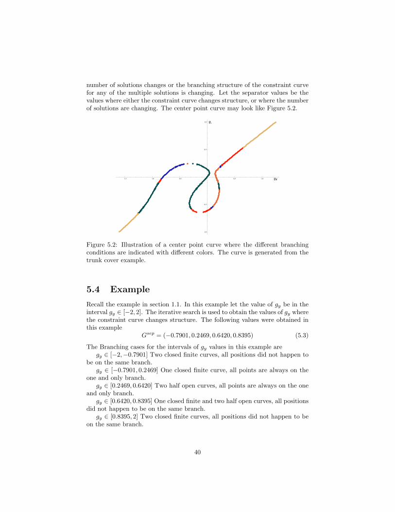
number of solutions changes or the branching structure of the constraint curvefor any of the multiple solutions is changing. Let the separator values be thevalues where either the constraint curve changes structure, or where the numberof solutions are changing. The center point curve may look like Figure 5.2.

1.5 1.0 0.5 0.5 1.0

1.0

0.5

0.5

1.0

gx

gy

Figure 5.2: Illustration of a center point curve where the different branchingconditions are indicated with different colors. The curve is generated from thetrunk cover example.

5.4 Example

Recall the example in section 1.1. In this example let the value of gy be in theinterval gy ∈ [−2, 2]. The iterative search is used to obtain the values of gy wherethe constraint curve changes structure. The following values were obtained inthis example

Gsep = (−0.7901, 0.2469, 0.6420, 0.8395) (5.3)

The Branching cases for the intervals of gy values in this example aregy ∈ [−2,−0.7901] Two closed finite curves, all positions did not happen to

be on the same branch.gy ∈ [−0.7901, 0.2469] One closed finite curve, all points are always on the

one and only branch.gy ∈ [0.2469, 0.6420] Two half open curves, all points are always on the one

and only branch.gy ∈ [0.6420, 0.8395] One closed finite and two half open curves, all positions

did not happen to be on the same branch.gy ∈ [0.8395, 2] Two closed finite curves, all positions did not happen to be

on the same branch.

40

Figure 5.3: All possible useful constraint curves to the four task positions fromthe car trunk demo.

5.5 Modifying the fifth task position

The initial problem where posted to find a strategy to modify a fifth task po-sition. However the exploration of all possible image curves to four positionsopens up new possibilities. An example of a task description could be to movethrough four task positions and avoid one or more points on the way. Thenthe line in the image space that describes this point for all orientations can becalculated, and the constraint curve that goes as far away from this line couldbe used.

If it is still desirable to have a fifth task position it can be done as well. Inthe classical synthesis methods the task positions are specified together with atolerance zone for x, y and θ. The tolerance zone is no longer of the same interestsince it from now on is possible to find the closest reachable task position.

The task positions in our case are assumed to be specified by the joint valuesof the first crank. Thus they will all lie on the first crank’s constraint manifold.Since the position consists of both translation and rotation, the closest distancehas to be defined. The importance of translation verses rotation will be specifiedby two weights w1 and w2.

It is assumed that a fifth task position should be reachable by the firstspecified crank. Therefore it has to lie on the surface of its constraint manifold.If the fifth task position is moved along the parametric curve defined by:

p5(t) = center(t) +

x0 ± w1tr(x0 ± w1t) cos(θ0 + w2t)r(x0 ± w1t) sin(θ0 + w2t)

(5.4)

the point will automatically stay on the constraint manifold. This curve is only

41

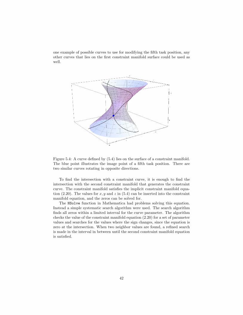
one example of possible curves to use for modifying the fifth task position, anyother curves that lies on the first constraint manifold surface could be used aswell.

Figure 5.4: A curve defined by (5.4) lies on the surface of a constraint manifold.The blue point illustrates the image point of a fifth task position. There aretwo similar curves rotating in opposite directions.

To find the intersection with a constraint curve, it is enough to find theintersection with the second constraint manifold that generates the constraintcurve. The constraint manifold satisfies the implicit constraint manifold equa-tion (2.20). The values for x, y and z in (5.4) can be inserted into the constraintmanifold equation, and the zeros can be solved for.

The NSolve function in Mathematica had problems solving this equation.Instead a simple systematic search algorithm were used. The search algorithmfinds all zeros within a limited interval for the curve parameter. The algorithmchecks the value of the constraint manifold equation (2.20) for a set of parametervalues and searches for the values where the sign changes, since the equation iszero at the intersection. When two neighbor values are found, a refined searchis made in the interval in between until the second constraint manifold equationis satisfied.

42

Chapter 6

Discussions

6.1 Adjusting to Primitive Shapes

The idea of adjusting the task positions to match some primitive shapes ofintersection curves did not show to be working. It did not show any significantdifferences in branching before and after adjusting the task positions. Also sincethe shapes were determined by looking at the intersection of two cylinders, theintersection of two hyperboloids will probably not take the exact same shape.The constraint curve for linkages synthesized did not either take a shape similarto the supposed primitive shape.

6.2 Structure interval

The linkage parameter gy was used to determine the structure intervals. As seenon the center point curve (Figure 5.2), the curve segments with small changes ofgy are not completed. This could possibly be solved by synthesizing by varyinganother linkage parameter such as gx instead. There is still much research to bedone before the most efficient and robust way of calculating all possible linkagesto four task positions is found.

6.3 Constraint Manifolds

The most interesting question is how to apply this theory on multiple-looplinkages. For a multiple-loop linkage, the constraint manifolds for each four-barloop in the linkage could be analyzed. This would give a set of constraint curvesin the image space. The constraint manifolds and constraint curve only tellswhich positions are reachable at some joint values. Since the joint values areeliminated when deriving the constraint manifolds, if the constraint manifoldsfor each four-bar loop in the linkage are analyzed, it would give a set of constraintmanifolds which may intersect in more positions than are reachable.

43

6.3.1 Order of Constraint Manifolds

The constraint manifold for a 2R chain is given by one equation. A curve in atwo-dimensional space is defined by one equation of any two coordinates vari-ables defining the plane. A plane in a three-dimensional space is defined byone equation of any three coordinate variables defining the space. One equationconstraints one variable, so one equation in a four-dimensional space will definea three-dimensional subspace which is the case for the 2R chain constraint man-ifold in the planar dual quaternion domain. While deriving the constraint mani-fold equation, the kinematics was described using two variables (the joint values)and four equations where given. From the first two equations q1 = cos

(θ2

)and

q2 = sin(θ2

), the condition q21 + q22 = 1. A similar condition could be obtained

from the third and fourth equation. The two variables where eliminated bythis and two equations remained. Those equations where subtracted from eachother to obtain the final constraint manifold equation. However one of the orig-inal two equations has to be saved. Only one of those where considered as theconstraint manifold equation but the trigonometric unity condition has to besatisfied as well to be a reachable position.

6.4 Synthesis of Non-Branching Six-Bar Link-ages

Exactly how this work can be applied on higher order of linkages is still unknown.For a multiloop linkage consisting of many four-bar linkages. The branchinganalysis can be applied to each four-bar. A constraint manifold equation canalso be derived for a 3R chain. However since a 3R chain has three degreesof freedom, the constraint manifold is a 3 dimensional region instead of a 2dimensional surface.

44

F1

F2

F0

F3

1

5

4

3

2

Figure 6.1: A Watt Ia six-bar linkage drawing from [6] with notations added on.

If the two constraint manifold regions C1−2−3 for link 1− 2− 3 and C4−5−3for link 4− 5− 3 are calculated, the intersection would give the work space forthe mechanism without link 2 and 4 connected.

A 3R chain 4−2−3 is considered, the intersection between the regions C1−2−3and C4−2−3 would be greater then the actual work space of the mechanism. Thereason is that the joint values of link 1 and link 4 is constrained by the four-bargenerated by links 1− 2− 4

It is an interesting future research topic how the constraint manifolds forfour-bar linkages stapled on top of each other will look. An approach I cansuggest for analyze the branching of a six bar is based on an assumption thatno four-bar sub-linkage in the assembly is allowed to branch.

45

Chapter 7

Conclusions

7.1 Kinematic Theory

7.1.1 Constraint Manifolds

The constraint manifold equation of a 2R chain was found to be a second degreehomogeneous polynomial equation. Since the constraint manifold equation is ahomogeneous equation, if it is satisfied by a planar dual quaternion Q, it is alsosatisfied by all multiples of the planar dual quaternion P = tQ. Therefore theconstraint manifold equation can be projected onto the kinematic image space.The constraint manifold equation describes a hyperboloid in the kinematic imagespace. The hyperboloid can be described by a center line and a radius. For eachx-value the constraint manifold forms a circle.

7.1.2 Constraint Curve of a Four Bar Linkage

A four-bar linkage can be constructed by two 2R chains with a common couplerlink (Figure 2.3). The constraint curve has to satisfy both constraint manifoldsof the two 2R chains. Since a constraint manifold forms a circle for a givenx-value, the constraint curve at that x-value (which is the intersection of twohyperboloids) will be the intersection of the two hyperboloids’ circles at thatx-value. Thus the constraint curve have zero, one or two points for each x-value.

Number of Intersection Points

There is exactly one intersection point at an x-value if the distance between thetwo center lines is the same as the difference or sum of the radius at the samex-value.

Solving for the constraint Curve

The constraint curve can be found by placing a coordinate system with origo onone of the constraint manifold’s center lines, with one coordinate axis pointing

46

at the other constraint manifold’s center line. In this coordinate system theintersection points can easily be solved for and the result can be transformedback to an inertial coordinate system.

7.2 Mechanism Branching

Between two x-values (split points) where the constraint curve has only oneintersection point, there is either no intersection of the manifolds between thosesplit points, or two intersection points for every x-value in between. Thus thebranching structure of a four-bar linkage can be determined by finding the splitpoints and checking the structure for only one point in each possible interval.

The split points divides the kinematic image space into a maximum of fourregions, which either includes a constraint curve for all x-values in the region,or does not include a constraint curve at all.

Figure 7.1: The image space is divided into a maximum of four regions whicheither contains a constraint curve for all x or no constraint curve at all.

It can be determined whether a linkage is useful by checking if all the taskpositions lie in the same region, if they do, the linkage is useful.

The region below the lowest plane and above the top plane is connectedtogether in infinity and is considered as one and the same region.

47

7.2.1 The Side of the Constraint Curve

In the case of two infinite curves, the branching is determined by which one ofthe curves the positions lies on. There can also be situations for closed curveswhere the side of the constraint curve is of interest. Which side a point lieson can be determined of transforming to a coordinate system located on onecenter line pointing to the other. The side is determined by the sign of one ofthe components.

7.3 Extruding all Possible Constraint Curves

By restricting the task specification to only allow four exact task positions,a large set of possible linkages could be found. If one linkage parameter isspecified, it can be determined for which values of the parameter the structureof the constraint curve changes. The structure intervals can then be calculatedfor the linkage parameter. If one linkage in a structure interval is useful, eitherall linkages in this structure interval are useful, or no linkages in the structureinterval are useful. The usefulness of a structure interval can then easily bedetermined by applying the branching test for any linkage in the interval.

7.4 Modifying a Fifth Task Position

A fifth task position has to lie on one of all possible constraint curves. Whenall possible constraint curves are calculated, the image point of a fifth task po-sition could be moved along a curve until it intersects with a possible constraintcurve. The curve to move along should be a curve on the first crank’s constraintmanifold, and is preferable determined by some weights constants determiningthe importance of the rotation verses translation of the task position.

7.5 Future Work and Research

It is still not well known which linkage parameter that is best to vary whilefinding the structure intervals. gy was used in this thesis but other parametersmight give higher accuracy. The next step would be to calculate all possibleconstraint curves without holding one crank fixed. Also a lot of computer pro-gramming has to be done to provide a robust algorithm. The suggested strategyof specifying zones or points to avoid by the mechanism could be implemented.The next interesting problem is to synthesize multiple loop linkages. If thesynthesis starts with specifying one chain and then constraining the chain withfour-bar linkages, then the branching of the four bars could be analyzed fordifferent dimension of the first chain. The goal would be to find all dimensionsfor which the first four-bar is not branching, then proceed to the second fourbar and find the dimensions for which the second is not branching either.

48

Appendix A

Dual Quaternions

This chapter contains my notes from learning and understanding dual numbersand dual quaternions. There are many papers written about quaternion anddual quaternions, however I found most of them very confusing and complicated.To understand the dual quaternions I found it useful to start with the most basicbuilding blocks and build up the understanding from there on.

A.1 Quaternions

The quaternions are mainly used for representing rotations, however they areat the same time a mathematical object which only represents a valid rotation.It is still of importance to start with the fundamental mathematics.

The quaternions will later on be considered as four-dimensional vectors.However the fundamental theory is based on the quaternions being scalar num-bers in the same as a complex number is a scalar number even though it hastwo dimensions and could be represented as a vector. The quaternions are fourdimensional hypercomplex numbers.

A.1.1 The Imaginary Dimensions

In the same way the imaginary unit i is introduced by the definition i2 = −1,two new imaginary dimensions will be introduced. Hamilton defined[8] therelationship between the products of the imaginary units to follow the rule:

i2 = j2 = k2 = −1 (A.1)

ij = k, jk = i, ki = j (A.2)

ji = −k, kj = −i, ik = −j (A.3)

An arbitary quaternion can be expressed as:

Q = q0 + q1i+ q2j + q3k (A.4)

49

or in a vector form:Q = (q0, q1, q2, q3) = (s,~v) (A.5)

where:~v = (q1, q2, q3) (A.6)

Some publications have the real part as the fourth element when represented asa vector.

Calculation laws

The calculation rules for quaternions follow by the standard calculation rulestogether with definition (A.1). The quaternion product expressed in a vectornotation is then:

Q1 ◦Q2 = (s1s2 − ~v1 · ~v2, ~v1s2 + s1~v2 + ~v1 × ~v2) (A.7)

The conjugate of a quaternion is (like the conjugate for a complex number) theimaginary parts inverted:

Q∗ = (q0,−q1,−q2,−q3) = q0 − q1i− q2j − q3k (A.8)

From (A.7), it follows that

Q ◦Q∗ =(q24 − ~v · (−~v,~vq4 + q4(−~v) + ~v × ~−v)

)= (0, ‖Q‖2) (A.9)

where ‖Q‖ is the euclidean norm of Q. All quaternions multiplied with it isconjugate is a real number. If ‖Q‖ = 1 the quaternion is a unit quaternion.

Application

A quaternion can be used for representing a three-dimensional rotation [17].

A.2 Dual Numbers

A dual number is a number involving the dual unit and consists of a real and adual part. It is similar to the complex numbers except that the dual unit ε hasthe property

ε2 = 0 (A.10)

The dual number also follows the commutative law. Let z1 = a1 + b1ε andz2 = a2 + b2ε be two dual numbers, and λ be a scalar. The following calculationrules follows from (A.10)

z1 + z2 = a1 + a2 + (b1 + b2)ε (A.11)

λz = λa+ λbε (A.12)

z1z2 = a1a2 + (a1b2 + a2b1)ε+ 0 (A.13)

50

Functions of dual numbers

To work with dual quaternions, we need to know about some functions of dualnumbers. The fundamental one is the exponential function. Taking the expo-nential of a pure dual number and expanding in a power series we get:

ebε = 1 + (bε) +(bε)2

2!+

(bε)3

3!+ · · · (A.14)

By definition in (A.10), all terms of power two or higher is zero, and we obtain:

ebε = 1 + bε (A.15)

The exponential of an arbitrary dual number is

ea+bε = eaebε = ea(1 + bε) (A.16)

The trigonometric functions of a dual number can be derived from the property

eiθ = cos(θ) + i sin(θ) (A.17)

Together with (A.16 ) we can write

ei(a+bε) = (cos(a) + i sin(a))(1 + biε) (A.18)

The dual valued functions of cos and sin can then be obtained from the real andimaginary part

cos(a+ bε) = Re(ei(a+bε)) = cos(a)− bε sin(a) (A.19)

sin(a+ bε) = Im(ei(a+bε)) = sin(a) + bε cos(a) (A.20)

A.3 Screw Displacement

An arbitrary three-dimensional displacement can be described by a screw. Thescrew consist of a unit screw axis, an angle and a distance. The displacementcorresponding to a screw with screw axis S, angle θ and distance d is obtainedby rotating the initial frame around the axis S by the angle θ at the sametime as the frame is translated along the axis by the distance d. We shall notethat the screw axis does not have to go through the origin. Thus it cannot berepresented by a single vector. Instead, the axis is represented by the pluckercoordinates for its line.

Plucker coordinates

A line specified by one arbitrary point C on the line and a direction vector ~S istransformed to plucker coordinates by:

L = (~S, ~C × ~S) (A.21)

The vector ~C × ~S is a vector which is normal to a plane that contains the lineand it has the length of the shortest distance from origo to the line.

51

A.4 Dual Quaternions

To represent an arbitrary three-dimensional displacement we can use a dualquaternion.

Such a displacement can be described by a rotation around the unit axes Sby an angle θ, and a translation along vector D = (x, y, z, 0) = xi + yj + zk.The dual quaternion for this displacement is

S = S +ε

2D ◦ S (A.22)

Given a dual quaternion S = A+ εB where A and B are quaternions. Withuse of (A.9), the translation vector can be found by:

D = 2B ◦A∗ (A.23)

Screw to quaternion

If the screw axis S intersects with origo, and the angle around S is θ anddisplacement along S is d, then the dual dumber for the screw is Θ = θ+ εd. Adual quaternion describing the screw is:

S = cos(Θ

2) + S sin(

Θ

2) (A.24)

The angle Θ is a dual angle. We use (A.19) and (A.20) to expand this to:

S = S sin(θ

2) + cos

θ

2+dε

2

(S cos(

θ

2)− sin(

θ

2)

)(A.25)

In case of a screw axis not intersecting origo, the vector S has to be theplucker coordinates for the screw axis. This is the case for the screw axisintersecting origo as well but in that case the dual part of the screw axis S iszero. Formula (A.24) is valid in both cases but for an arbitrary screw axis it isexpanded into a more complex expression.

Displacement Chain

In many cases, e.g. robot kinematics, we want to apply a number of transfor-mations after eachother to finaly reach the end effector position. By havingeach transformation represented by the dual quaternions Qi, the end effectorposition QTCP is obtained by:

QTCP =

n∏i=1

Qi (A.26)

52

A.5 Notations

· dot product (euclidean norm inner product)◦ quaternion multiplication⊗ dual quaternion multiplication× cross product (Vector product)Q∗ conjugate of quaternion

53

Bibliography

[1] J. Mervelet, “American airlines boeing 767-323/er,”http://www.airliners.net/photo/American-Airlines/Boeing-767-323-ER/1208702/S/, March 2007.

[2] R. D. Dean, “Three-position variable camber flap,” U.S. Patent 4 262 868,1981. [Online]. Available: http://www.google.com/patents/US4262868

[3] G. T. Brine, “Flap mechanism,” U.S. Patent 4 542 869, 1983. [Online].Available: http://www.google.com/patents/US4542869

[4] Formula Student, http://www.formulastudent.com/.

[5] LU Racing, “Lund University’s Formula Student Team,”http://www.luracing.se, 2012.

[6] J. M. McCarthy, Geometric Design of Linkages. Springer, 2001.

[7] ——, An Introduction to Theoretical Kinematics. MIT Press.

[8] W. R. Hamilton, “On quaternions, or on a new system of imaginaries inalgebra,” Philosophical Magazine, 1844.

[9] J. Grunwald, “Ein abbildungsprinzip, welches die ebene geometrie undkinematik mit der raumlichen geometri verkupft,” Sitzber. Ak. Wiss. Wien,1911.

[10] O. Bottema and B. Roth, Theoretical kinematics. North-Holland Press,1979.

[11] T. R. Chase and J. A. Mirth, “Circuits and branches of single-degree-of-freedom planar linkages,” ASME Journal of Mechanical Design, 1993.

[12] B. Parrish and J. M. McCarthy, “Identication of a usable six-bar linkagefor dimensional synthesis,” 2012.

[13] H.-P. Schrocker, M. Husty, and J.M.McCarthy, “Kinematic mapping basedevaluation of assembly modes for spherical four-bar synthesis,” in Proceed-ings of ASME 2005 29th Mechanism and Robotics Conference, Long Beach,CA, 2005.

54

[14] H.-P. Schrocker, M. Husty, and J. M. McCarthy, “Kinematic mapping basedevaluation of assembly modes for planar four-bar synthesis,” in Proceedingsof EuCoMeS, the first European Conference on Mechanism Science, feb2006. [Online]. Available: http://geometrie.uibk.ac.at/eucomes/eucomes-sample.pdf

[15] J. W. Gibbs, Elements of vector analysis. Tuttle, Morehouse & Taylor,1884.

[16] J. M. McCarthy, Geometric Design of Linkages. Springer, 2001.

[17] J. B. Kuipers, Quaternions and Rotation Sequences: A Primer with Ap-plications to Orbits, Aerospace and Virtual Reality. Princeton UniversityPress, August 2002.

55