brain vs. brawn: child labor, human capital investment, and the … · 2019-03-04 · brain vs....
TRANSCRIPT

Brain vs Brawn Child Labor Human Capital Investment and the
Role of Dynamic Complementarities
Natalie Bau
UCLA and CEPR
nbauuclaedu
Martin Rotemberg
New York University
mrotembergnyuedu
Manisha Shah
UCLA and NBER
ManishaShahuclaedu
Bryce Millett Steinberg
Brown University
bryce steinbergbrownedu
February 11 2019
Abstract
Early-life interventions are a promising route to improve educational outcomesYet in many low-income countries children (and their parents) make trade-offs be-tween schooling and productive work We formalize this trade-off in a simple model ofhuman capital investment If early-life investments increase child wages more than theyincrease the returns to education children who receive greater early life investmentswill attend less school Exploiting rainfall shocks as a source of variation in early-lifeincome in India we test the model Parental income shocks early in a childrsquos life leadto higher educational attainment in places with low levels of child labor but this pos-itive effect is attenuated in areas with high child labor When child labor is especiallyprevalent positive early shocks have statistically significant negative effects on educa-tional attainment To verify that this is not driven by the unobservable characteristicsof high child labor regions we replicate this pattern using geographic variation in twochild labor intensive crops cotton and sugar
JEL Codes O12 I2 J1
We would like to thank seminar participants at UCSD NYU and Dartmouth for helpful comments andquestions Shah and Steinberg acknowledge funding from NSF grant 1658852
1 Introduction
Policies that increase human capital investment during the critical period ages zero to five
when the developing brain is most plastic (Knudsen et al 2006) are a promising tool to
increase overall human capital attainment Beyond the high returns of these early interven-
tions a growing literature focusing on ldquodynamic complementaritiesrdquo in the human capital
production function suggests that early skills beget more skills by increasing the returns
of later human capital investments (Cunha and Heckman 2007 Gilraine 2017 Agostinelli
and Wiswall 2016 Johnson and Jackson 2017) However in places where children and
adolescents work productively (in the market on the family farm or in home production)
if there are returns to human capital in that work a higher initial stock of human capital
could increase the costs of educational investments as well Thus actions taken by parents
and children can undo the positive educational effects of these interventions by altering their
human capital investments in response to positive early-life shocks (Malamud et al 2016)
While much of the literature on early-life investment has focused on these investments in
high-income countries1 understanding how parents and children respond to positive early-
life shocks is particularly important in low-income countries where child labor is common
(Bharadwaj et al 2013)
In this paper we provide novel evidence that increased early-life health inputs also in-
crease the opportunity cost of schooling by increasing the returns to child labor in rural India
Thus the direction of the effect of early-life investments on educational and even long-term
wage outcomes will depend on two countervailing forces (1) how much the early-life invest-
ments increase the returns to child labor and (2) how much they increase the returns to
later educational investments (the size of dynamic complementarities) By increasing the
opportunity cost of schooling the existence of child labor can mitigate the positive effects of
early-life shocks on later schooling In extreme cases positive early life human capital shocks
1Attanasio et al (2015) which estimates the human capital production function in India is a notableexception
1
can actually reduce overall schooling levels In contrast with the literature on high-income
countries early life human capital investments aiming to increase long-run human capital
accumulation may be counter-productive in low-income contexts with high child labor
To formalize this intuition we first develop a simple three-period theoretical model of
human capital investment that allows for both dynamic complementarities in human capital
investment and a positive effect of a childrsquos human capital on his or her child labor wages
Then to test the predictions of the model following Maccini and Yang (2009) and Shah
and Steinberg (2017) we use variation in rainfall shocks when a child is young (in utero
to age 2) as an exogenous shock to the initial stock of human capital In line with the
previous literature we first show that positive rainfall shocks result in greater weight height
and school-age test scores indicating that positive shocks improve early-life human capital
investment Additionally we show that children who experience these positive shocks and
work for a wage receive higher wages indicating that these early-life shocks positively affect
the return to work rather than attending school
Consistent with the existence of dynamic complementarities we find that positive early-
life income shocks increase the likelihood that a child attends school when he or she is
school-aged in areas with low baseline levels of child labor However this positive effect
is attenuated in districts with higher baseline levels of child labor In districts in the top
quintile for baseline levels of child labor the sign is reversed and the overall effect of a
positive income shock in early-life on education is significantly negative for schooling
Since high child labor districts may differ from low child labor districts on a variety of
dimensions we then show that our results are robust to utilizing variation in the pervasive-
ness of child labor induced by ldquotechnological variationrdquo We focus on sugar and cotton two
crops known to be labor intensive and particularly prone to using child labor Using adult
shares of employment in these industries we classify districts as sugar or cotton produc-
ers and find that being a sugarcotton producer is highly predictive of child labor levels
When we compare the effects of positive early life rainfall in these districts to the effects
2
in non-sugarcotton producers we find the same pattern as before In sugar and cotton
producing districts the positive early-life investments facilitated by positive rainfall shocks
decrease the likelihood of attending school during childhood In non-sugarcotton producing
districts the opposite is the case
Our results stress the importance of accounting for the effect of early-life investments
on the opportunity cost of schooling as well as the returns to schooling in low-income
countries From a policy perspective If the policymakerrsquos objective is to increase schooling
investing in early-life interventions without complementary interventions to reduce child
labor may be counterproductive Taking the effect of early-life investments into account
is also important for researchers characterizing the human capital production function in
low-income countries If we draw inferences about the human capital production function
from high child labor areas without taking into account the opportunity cost of schooling
we would falsely conclude that later human capital investmentsrsquo returns are decreasing in
early investments On the other hand if we focus on low child labor areas our results would
be consistent with dynamic complementarities
These results contribute to a growing literature on the opportunity cost of schooling
in both developed (Charles et al 2015 Cascio and Narayan 2015) and developing coun-
tries (Shah and Steinberg 2017 2018 Atkin forthcoming) This paper is also related to
the literature on dynamic complementarities which was theoretically introduced by Cunha
and Heckman (2008) and tested empirically in several different contexts (Gilraine 2017
Agostinelli and Wiswall 2016 Johnson and Jackson 2017 Cunha and Heckman 2007)
While our paper does not directly test for the presence of dynamic complementarities in the
human capital production function we do illustrate an important additional channel through
which earlier human capital investments might impact later schooling choicesmdashchild labor
The paper proceeds as follows Section 2 provides further background on child labor
in India and describes the data used in the analysis in this paper Section 3 describes the
theoretical framework Section 4 presents our empirical strategy and tests the predictions of
3
the model for wages education and child labor allowing early-life shocks to have differential
effects by the baseline child labor in a district Section 5 concludes
2 Background and Data
21 Background on Child Labor in India
Although child labor for children 14 and under was officially banned in India in 1986 the
ban covered only certain industries and was not well enforced2 Importantly agriculture and
family-run businesses ndash perhaps the chief employers of child labor ndash were exempted from the
ban Beyond the various exemptions there is some evidence that the ban itself may have
increased child labor through negative income effects (Bharadwaj et al 2013)
Overall child labor is common in India as it is in many low-income countries According
to the NSS 5 of children under 18 report working as their primary activity while 22
of individuals 15ndash17 do so Figure 1 shows the variation in the percent of children under
18 who report working as their primary activity across Indian districts The most common
industries for these children are agriculture and construction Shah and Steinberg (2017)
show that child labor responds to productivity shocks suggesting that wages are an impor-
tant determinant of whether children work Finally while some children work in the labor
market for pay most work part-time at home or on family farms
22 Data
221 Main Outcomes Child Labor School Attendance
We use the National Sample Survey (NSS) to measure our main outcomes of interest school
attendance and work The National Sample Survey is a repeated cross section of an average
2Industries banned included occupations involving the transport of passengers catering establishmentsat railway stations ports foundries handling of toxic or inflammable substances handloom or power loomindustry and mines Processes banned included hand-rolling cigarettes making or manufacturing matchesexplosives shelves and soap construction automobile repairs and the production of garments (Bharadwajet al 2013)
4
of 100000 Indian households a year conducted by the Indian government We use Schedule
10 (Employment and Unemployment) from rounds 60 61 62 and 64 (2004 2004-5 2005-6
and 2007-8) in our main analysis The survey asks each member of the household for their
ldquoprimary activityrdquo and includes categories for school attendance wage labor salaried work
domestic work etc We count a child as ldquoattending schoolrdquo if their primary activity is listed
as attends school and ldquoworksrdquo if their primary activity is any form of wagesalary labor
work with or without pay at a ldquohome enterpriserdquo (usually a farm but also includes other
small family businesses) or domestic chores These two categories comprise most of the
primary activities of children under 18 though there are other categories that are omitted
such as too younginfirm for work (typically the very old and very young) and ldquootherrdquo
which includes begging and prostitution
In addition in order to understand whether the interaction between early-life investment
and the presence of a market for child labor can affect the opportunity cost of schooling
we need a measure of child labor by district For that measure we use the 2000 (round 57)
NSS Our primary measure of child labor is the fraction of children (age 0-18) who report
their primary activity as work in a district We will also use the share of cotton and sugar
production in the district (since those two crops have the highest proportion of child workers)
as a proxy for child labor
222 Secondary Outcomes Child Labor Wages Test Scores and Anthropometrics
For additional data on child labor wages and activities we turn to the India Human Devel-
opment Survey (IHDS) a repeated panel dataset that was implemented in 2005 and 2012
This survey also measures child height weight and cognitive abilities and these data allow
us to test the assumption that children with higher human capital earn higher wages in the
market We further supplement the IHDS and the NSS with data from ASER which in-
cludes test scores for a large cross-section of children ndash including those who are out of school
ndash from 2005ndash2009
5
223 Variation in Human Capital Yearly Gridded Rainfall
Our data on rainfall shocks come from the University of Delaware Gridded Rainfall Data for
1970-2008 Following earlier literature (Shah and Steinberg 2017 Jayachandran 2006) we
define a ldquorainfall shockrdquo as equal to one if rain is in the top 20th percentile for the district
-1 if it is in the bottom 20th percentile and 0 otherwise3 We match this data to children in
the NSS the IHDS and ASER by their birth year at the district level To verify that our
implicit first-stage (that rainfall affects agricultural wages) is relevant we also match this
data to World Bank data on crop yields from 1975ndash1987
Table 1 documents our different data sources and the key variables from each source
3 Model
We develop a simple model of human capital investment in the presence of child labor The
model clarifies the circumstances under which positive early-life human capital investments
can reduce schooling even in the presence of dynamic complementarities in the human
capital production function We first show that the early-life income shocks caused by
positive rainfall shocks lead to increased early-life human capital investment If there are
dynamic complementarities this human capital investment positively affects the returns to
later schooling investment incentivizing parents to invest more in later-education However
in places where child labor is prevalent early-life investments also affect the child wage
which is the opportunity cost of schooling This countervailing force attenuates the positive
effect of early-life investment on schooling In extreme cases early-life investments increase
the child wage more than they increase the returns to education causing schooling to fall
We document this with greater formality in the next two sub-sections which first present
the set-up of the model and then derive propositions
3In India though flooding does happen more rain is almost always better for crop yields This is welldocumented in Jayachandran (2006)
6
31 Set Up
The decision-maker in the model is a parent and each parent has one child The decision-
maker is indexed by her childrsquos educational ability α which is distributed according to the
function F and her type of district d isin low high d denotes whether a parent is in a
high or low child labor district There are three periods in the childrsquos life early life school
age and adulthood and α becomes observable in period 2 when a child is old enough to
attend school The parent lives for the first two periods In period 1 they decide how
much to invest in a childrsquos early-life human capital h In period 2 they make a discrete
decision whether or not to educate the child e isin 0 1 or have the child work for a wage
wc2d(h) Child wages depend on both early-life investment h and d The discrete educational
investment maps to the fact that children either primarily work or attend school in our data
rather than moving between working and education on a continuum The parent consumes
in both periods and also have some altruism toward their childrsquos third period adult utility
Suppressing the indices α and d a parentrsquos preferences in period 1 are represented by
Up1 (h) = u(cp1(y1 h)) + E
983059max
eu(cp2(y2 e h)) + δU c(cc3(e h))
983060
where cp1 and cp2 are the parentrsquos consumption in periods 1 and 2 cc3 is the childrsquos adult
consumption in period 3 u is the utility function U c is the childrsquos adult utility which
depends on educational and early-life investments δ is the product of the parentrsquos discount
rate and her altruism toward the child and the expectation is taken over realizations of α
Both u and U c are assumed to have diminishing marginal returns in consumption
Similarly the parentrsquos period 2 utility is given by
Up2 (h e) = u(cp2(y2 e h)) + δU c(cc3(e h))
For simplicity the model abstracts away from borrowing and saving Then parental con-
7
sumption in period 1 is equal to some exogenous income y1 net the cost of human capital
investment h Parental consumption in period 2 is total income y2 net the cost of schooling
if e = 1 or plus the wages from child labor if e = 0 Thus
cp1 = y1 minus chh
cp2 = y2 + (1minus e)wc2d(h)minus cee
cc3 = wc3(e h) + αe
where ch is a cost of the human capital investment and ce is the cost of education wc3(e h)+αe
is the childrsquos total adult wage where the function wc3(e h) allows for a flexible relationship
in adult wages between e and h Following Cunha and Heckman (2008) there are dynamic
complementarities in the adult wage function ifpartwc
3(1h)
parthgt
partwc3(0h)
parth This captures the idea
that early life investments in human capital make educational investments more productive
The wage expression also allows children to heterogeneously benefit from schooling based on
their schooling ability α
Before solving the model we make several assumptions to simplify exposition First
we assume that wc2low(h) = 0 so that if child labor in a district is negligible child wages
are always equal to zero In places where child labor is high we assumepartwc
2high
parthgt 0 This
assumption captures the idea that early-life human capital investments increase child wages
We directly test this assumption in our data in the next section
32 Predictions
We now solve for the parentrsquos equilibrium investment decisions and relate them to changes
in first period income y1
Proposition 1 Denote hlowast as the parentrsquos equilibrium choice of h If wc2d(h) and wc
3(e h)
have diminishing marginal returns in hparthlowast
d
party1gt 0 foralld
Proof See Appendix A
8
The first proposition indicates that a positive income shock in early life will increase
early-life human capital investment The intuition for this prediction is straightforward
When y1 increases the marginal utility of first period consumption falls increasing the
parentrsquos incentive to invest in her childrsquos human capital This proposition is consistent with
the previous findings of Shah and Steinberg (2017) and Maccini and Yang (2009) who show
that an early life shock increases test scores and weight
Building on Proposition 1 the next set of propositions develop the key predictions of
the paper ndash that early life shocks increase education rates in places with low child labor and
have no effect on or even decrease education rates in places with high child labor
Proposition 2 Denote λd(y1) to be the share of children educated in a district of type d
given y1partλlow(y1)
party1gt 0 only if
partwc3(1h)
parthgt
partwc3(0h)
parth
Proof See Appendix A
This proposition captures the fact that in low child labor places increased h only posi-
tively affects the parentrsquos educational decisions through its effect on the returns to later-life
educational investments Therefore if an early life shock increases educational investments
in low child labor markets this is evidence in favor of the fact that early life investments
increase the returns to later educational investments However as predictions 3a and b
show in high child labor markets positive early life investments can have zero or negative
effects despite their potential positive effect on the returns to education due to dynamic
complementarities
To introduce Proposition 3a we first note that for a given value of h the parent will
educate a child if Up2 (h 1) ge Up
2 (h 0) Since partUp(h1)partα
gt 0 and partUp(h0)partα
= 0 this relationship
exhibits single-crossing Thus for any combination of h and d there exists a cut-off value
αlowastd(h) for α where e = 1 for all children with α ge αlowast
d(h) Figure 2 illustrates this by plotting
the ability distribution F and showing that e = 1 if α gt αlowastd(h)
Proposition 3a Iff(αlowast
high(hlowasthigh(y1)))
f(αlowastlow(hlowast
low(y1)))lt Φ
partλhigh(y1)
party1lt partλlow(y1)
party1forallI
9
Proof See Appendix A
This proposition indicates that a positive income shock increases education (and adult
wages) more in low child labor districts than high child labor districts as long as the fact
that increased returns to the parent from child labor dominate two other second order
effects with ambiguous directions This is captured by the assumptionf(αlowast
high(hlowasthigh(y1)))
f(αlowastlow(hlowast
low(y1)))lt Φ4
The effect we expect to dominate is that an increase in h increases the relative returns to
education more in low child labor areas because in high child labor areas increasing h also
increases the outside option wc2d The additional ambiguous effects come from the fact that
(1) the density of children on the margin of being educated is different in high and low child
labor regions since enrollment rates are different and (2) the derivative of adult wages with
respect to early childhood investment may be different in high and low child labor regions
if underlying investment in h is different in these regions If underlying early-life human
capital investment rates are similar and the densities of the distribution at αlowastd(hd(y1)) are
similar across these regions these additional effects will be small5
Figure 3 illustrates the intuition for proposition 3a In both high and low child labor
districts the increase in y1 increases the relative returns to schooling causing αlowastd(h
lowastd)) to
fall But αlowastlow falls more than αlowast
high because the relative returns to schooling increase more in
low child labor districts The share of children whose educational outcomes are changed is
captured by the gray areas which integrate over the ability distribution from the old to the
new values of αlowastlow and αlowast
high Even though the density at the cut-off is different in high and
low child labor districts as long as it is not too much greater in high child labor districts more
children will be affected in low child labor districts where the integral is taken over a larger
set of values of α While proposition 3a shows that the effects of early-investment on the
4Φ =
partwc3(hlowast
low1)
party1minus
partwc3(0hlowast
low)
party1Ucprime(wc
3(0hlowastlow))
Ucprime(wc3(1hlowast
low)+αlowast
low)
partwc3(1hlowast
high)
party1minus
uprime(y2+wc2high
(hlowasthigh
))partwc
2d(hlowast
high)
party1+δ
partwc3(0hlowast
high)
party1Ucprime(wc
3(hlowasthigh
0))
δUcprime(wc3(1hlowast
high)+αlowast
high)
5The assumption thatf(αlowast
high(h(y1)))
f(αlowastlow(h(y1)))
lt Φ bounds how much greater the density at αlowastlow can be relatively
to the density at αlowasthigh That is if the density at αlowast
high is sufficiently high it can lead the response to shocksto be greater in high child labor places even though the change in the ability cut-off is smaller
10
returns to child labor can attenuate the positive effects of early-life investment on schooling
the next proposition shows that in extreme cases early-life investment can negatively affect
schooling
Proposition 3b Ifpartwc
2high(hlowast(y1))
parthis sufficiently great
partλhigh(y1)
party1lt 0
Proof See Appendix A
Proposition 3b shows that when the effect on parental utility of the increase in child
wages due to an increase in y1 is sufficiently large in high child labor places it outweighs
the effect of the increase in the returns to education (weighted by the parentsrsquo altruism and
discount rate) Then positive income shocks that increase early life investments can lead to
reduced education potentially translating into reduced wages later in life
4 Empirical Strategy and Results
Our model predicts that children with different initial levels of human capital will make
different choices to invest in schooling and that these choices can depend on the economic
environment To identify these effects we need variation in both the initial stock of human
capital and the labor market for children We will address these issues step-by-step First
in Section 41 we will show that rainfall shocks experienced early in life provide a plausibly
exogenous shock to the initial stock of human capital consistent with previous work (Maccini
and Yang 2009 Shah and Steinberg 2017) In Section 42 we show that these differences
in human capital affect child wages and thus their opportunity cost of education Secondly
in Section 43 we show that these differences in the initial stock of human capital cause
differential investment in education during childhood Third in Section 43 we show that
these responses to human capital stock differ based on the prevalence of child labor in the
districtmdashin places with low child labor children with high initial stocks of human capital
are significantly more likely to be in school during childhood and in places with the highest
child labor children are less likely to be in school and more likely to be working This is
11
consistent with both dynamic complementarities in the human capital production function
and a return to human capital in the market for child labor Lastly in Section 44 we use
crop shares as a more exogenous source of variation in child labor and find similar results
41 Variation in Early-Life Human Capital
To test the implications of the model we use early life rainfall shocks as a proxy for shocks
to early-life human capital The existing literature provides a strong argument for this rela-
tionship The argument is as follows positive rainfall shocks increase yield which increases
parental wages as shown by Jayachandran (2006) and Kaur (forthcoming) Intuitively and
as we also demonstrate in Prediction 1 of our model higher parental wages lead to higher
early-life investment (Maccini and Yang 2009 and Shah and Steinberg 2017) This could
take the form of increased nutrition for pregnant or breastfeeding mothers increased medical
care during infancy more parental time spent fostering development etc
Our data are consistent with these hypotheses As Appendix Table A1 shows positive
rainfall shocks increase yield Here a rainfall shock is coded as 1 if rain is greater than
the 80th percentile of the distribution from 1975 to 2008 minus1 if it is less than the 20th
percentile and 0 otherwise following Jayachandran (2006) Furthermore we replicate the
positive relationship between rainfall and wages found in the literature in Appendix Table
A2
We next aggregate rainfall shocks into a single child-level measure by taking the sum
across the three shocks in-utero age 1 and age 2 Tables 2 and 3 also confirm that early-life
shocks affect human capital in our data showing that children who experience shocks in
utero in their first year and in their second year have higher height and weight in the IHDS
(Table 2) and better test scores in the ASER (Table 3) These findings confirm Prediction 1
from the model and show that rainfall shocks are a relevant instrument for early-life human
capital investment
12
42 Early Human Capital Investments Affect Child Wages
We next turn to the key assumption of our model that early-life human capital investments
affect the opportunity cost of schooling by increasing child wages To test whether this is
the case we first use the IHDS to regress child wages on human capital measures with the
following specification
yidta = αa + β1human capidta + ΓXi + 983171idta
where i denotes a child a denotes age t denotes the survey round d denotes a district αa is
an age fixed effect and Xi is the set of controls consisting of gender and district fixed effects
human capi is our human capital measure which may be height weight or lagged math
scores Thus β1 is our coefficient of interest and we expect it to be positive We restrict
our sample to individuals aged 0ndash17 and cluster our standard errors at the district-level
Since our proxies for human capital are likely endogenous we next instrument for height
using our child-level aggregate rainfall shock measure Our first stage regression is then
human capidta = αa + λ1ELRdta +ΨXi + υidta
where ELRiat is the aggregate rainfall measure
Table 2 reports the results of these regressions In both the OLS and the IV we find
a positive relationship between child wages and measures of human capital supporting the
key assumption of the model that human capital investments also affect the outside option
43 Early-Life Investment and Schooling
We now turn to testing the key prediction of our model Based on Prediction 2 we expect
that if there are dynamic complementarities in districts with low child labor early life shocks
will increase educational investment In districts with high child labor this effect will be
13
attenuated (Proposition 3a) and may even be reversed (Proposition 3b) so that early-life
shocks decrease human capital investment
We first show graphical evidence that this is the case in Figures 4 and 5 Figure 4 shows
the effect of an early life rainfall shock on school attendance for children under 17 separately
by the district quintile of average child labor at baseline In places with low baseline child
labor positive early rainfall shocks increase school enrollment later in childhood However
as child labor increases this effect attenuates and in the districts in the highest quintile of
child labor the effect is reversed so that children with positive early life shocks are less likely
to be in school Figure 5 shows the opposite pattern for childrenrsquos work in low child-labor
districts children with positive shocks to human capital are less likely to be working but in
high child-labor districts they are significantly more likely to be working
To test whether this is the case we estimate the following regression
yidta = αa + β1ELRdta + β2ELRdta times CLd + γd + δt + 983171idta (1)
where yidta now consists of measures of working or being enrolled in school CLd is a measure
of the child labor in the district (either the percent of children engaged in child labor in the
NSS or an indicator variable for the percent being over a cut-off value) γd is a district fixed
effect and δt is a survey year fixed effect The remaining variables and subscripts are defined
as before
From Prediction 2 we expect β1 to be positive if there are dynamic complementarities
Prediction 3a predicts that β2 lt 0 indicating that the increase in child wages due to early-
life human capital investments reduces the positive effect of early-life human capital on
investment Prediction 3 suggests that cases may exist where β1 + β2 lt 0 indicating that
the effect of early-life human capital investment on child wages dominates the effect on the
returns to education
Table 5 reports the results of these regressions In Panel A we report estimates for the
14
effect of early life rain on whether a childrsquos primary activity is attending school On average
children who experience one more positive rain shock early in life are about 03 percentage
points more likely to attend school each year As this is the estimated effect on enrollment
for the average year over the course of the 17 years of child life included in the sample this
would lead to a 0051 year increase in schooling However in districts with more child labor
this effect is attenuated In fact in the districts in the top quintile of child labor children
who experience more rainfall early in life are significantly less likely to attend school Each
year a child who receives one more positive rainfall shock is 07 ppt less likely to be enrolled
Aggregating up this is a 012 year decrease in a childrsquos schooling For comparison a large
primary school construction program in Indonesia increased male schooling by 012 years
(Duflo 2001) suggesting that these effects are meaningful
In Panel B of Table 5 we replace school with work as the childrsquos primary activity for
the outcome variable The effects are similar Children in low child labor districts reduce
the likelihood of reporting working by 03 ppt suggesting they work 005 fewer years as a
result of one additional year of positive rainfall early in life Children in high child labor
places are 09 ppt more likely to work implying that they spend 0153 more years working in
aggregate The similarly sized (but opposite) effects on working and education suggest that
the positive early-life shocks mainly affect children on the margin between work and school
One potential threat to the validity of these estimates is that baseline child labor levels
may be correlated with an omitted variable that causes early life shocks to have smaller
(or negative) effects on education for other reasons Two of the most intuitive candidate
omitted variables are income and school quality For income high child labor areas could be
poorer so parents are less able to complement positive early-life shocks with later educational
investments or complementarities between schooling and educational investment could be
smaller because fewer high skilled jobs are available Similarly areas with high child labor
could have lower school quality reducing the complementarity between early life human
capital and education and therefore reducing parentsrsquo incentives to invest in education To
15
account for income we calculate the average adult wage and share of those who work for
a wage for each district at baseline and include the interaction between these controls and
ELRdta in equation (1) To account for school quality we take the average literacy rate in
each district and the primary and secondary school completion rates and also include these
interactions with ELRdta Figures 6 and 7 report the total effect of an early life shock in a
top quintile child labor district (β1 + β2CLd) for these new specifications For both working
and attending school the results are qualitatively similar to those without the controls
Figures 8 and 9 further explore the distribution of the effects of early-life shocks on
education and child labor across age groups These figures are generated by interacting
ELRdta and ELRdtatimesCLd with age fixed effects in equation (1) We then report estimates of
the total effect of a positive shock on education and working by age for children in districts in
the top quintile for child labor Consistent with the intuition of the model children exposed
to more positive early life rainfall shocks are neither more likely to work nor drop out until
the early stages of adolescence If anything preadolescent children exposed to early life
rainfall shocks are more likely to remain in school even in high child labor districts
44 Crop Variation as a Proxy for Child Labor
The share of children working in a given district is itself an equilibrium outcome caused by
various attributes of the district and the people who live there While in the previous section
we do not find that our measures of poverty or schooling qualitatively change the patterns
it is possible that we are measuring the (potential) confounders with error and that they
cause the differences in the response of education to early life shocks rather than child labor
itself To address this we take advantage of the fact that some crops are easier for children
to work on than others given the nature of the tasks associated with planting weeding and
harvesting the crops In the NSS cotton and sugar are the two crops that have the highest
proportion of workers under 18 (around 15 of workers in each crop are children at the start
of our sample) This is consistent with other contexts cotton in particular is notorious as a
16
child labor crop because it is low to the ground and very lightweight (Levy 1985) Cotton
and sugar both require somewhat specialized growing conditions and thus grow in only 20
of districts in India
We use both the presence of any sugar or cotton crop and the percentage of acreage in
the district of each of these crops as a proxy for child labor In Table 6 we re-estimate
our results from Table 5 using this proxy in place of district averages for child labor These
results tell a very similar story On average children who experience better early life rain
are less likely to be working and more likely to be attending school However in places with
cotton and sugar these effects are reversed and children who experience higher early life
rain are less likely to be in school and more likely to be working
5 Conclusion
Interventions that increase early-childhood investment may be a powerful tool for increasing
educational attainment overall However such policies could have counter-intuitive effects in
low-income countries where child labor is common We provide new evidence that early-life
investments increase child wages increasing the attractiveness of child labor Furthermore
we document the fact that while early-life investments positively affect educational outcomes
in places where child labor is low consistent with the existence of dynamic complementarities
this effect is attenuated in places where child labor is high In the places where child labor
is the highest early life interventions may even reduce long-term educational outcomes
These results have important implications both for policy-makers interested in increasing
educational outcomes and for researchers interested in identifying the form of the human
capital production function For the latter our results suggest that researchers particularly
those working in low-income countries must take into account how child human capital
affects the opportunity cost of schooling as well as the benefits of schooling
17
References
Agostinelli Francesco and Matthew Wiswall ldquoEstimating the Technology of Childrenrsquos SkillFormationrdquo NBER Working Paper 2016
Atkin David ldquoEndogenous Skill Acquisition and Export Manufacturing in Mexicordquo AmericanEconomic Review forthcoming
Attanasio Orazio Costas Meghir and Emily Nix ldquoHuman capital development andparental investment in indiardquo Technical Report NBER Working Paper 2015
Bharadwaj Prashant Leah K Lakdawala and Nicholas Li ldquoPerverse consequences of wellintentioned regulation evidence from Indiarsquos child labor banrdquo NBER Working Paper No 196022013
Cascio Elizabeth U and Ayushi Narayan ldquoWho Needs a Fracking Education The Ed-ucational Response to Low-Skill Biased Technological Changerdquo 2015 NBER Working Paper21359
Charles Kerwin Kofi Erik Hurst and Matthew J Notowidigdo ldquoHousing Booms andBusts Labor Market Opportunities and College Attendancerdquo 2015 NBER Working Paper21587
Cunha Flavio and James Heckman ldquoThe Technology of Skill Formationrdquo American EconomicReview Papers and Proceedings May 2007 97 (2) 31ndash47
and James J Heckman ldquoFormulating Identifying and Estimating the Technology of Cog-nitive and Noncognitive Skill Formationrdquo Journal of Human Resources 2008 43 (4) 738ndash82
Duflo Esther ldquoSchooling and Labor Market Consequences of School Construction in IndonesiaEvidence from an Unusual Policy Experimentrdquo The American Economic Review 2001 91 (4)795
Gilraine Mike Working Paper 2017
Jayachandran Seema ldquoSelling Labor Low Wage Responses to Productivity Shocks in Devel-oping Countriesrdquo Journal of Political Economy 2006 114 (3)
Johnson Rucker C and C Kirabo Jackson ldquoReducing Inequality Through Dynamic Comple-mentarity Evidence from Head Start and Public School Spendingrdquo Technical Report NBERWorking Paper 2017
Kaur Supreet ldquoNominal Wage Rigidity in Village Labor Marketsrdquo American Economic Reviewforthcoming
Knudsen Eric I James J Heckman Judy L Cameron and Jack P Shonkoff ldquoEconomicneurobiological and behavioral perspectives on building America s future workforcerdquo Proceedingsof the National Academy of Sciences 2006 103 (27) 10155ndash10162
Levy Victor ldquoCropping pattern mechanization child labor and fertility behavior in a farmingeconomy Rural Egyptrdquo Economic Development and Cultural Change 1985 33 (4) 777ndash791
18
Maccini Sharon and Dean Yang ldquoUnder the Weather Health Schooling and EconomicConsequences of Early-Life Rainfallrdquo American Economic Review June 2009 99 (3) 1006ndash26
Malamud Ofer Cristian Pop-Eleches and Miguel Urquiola ldquoInteractions Between Familyand School Environments Evidence on Dynamic Complementaritiesrdquo Technical Report NBERWorking Paper 2016
Shah Manisha and Bryce Millett Steinberg ldquoDrought of Opportunities Contemporaneousand Long Term Impacts of Rainfall Shocks on Human Capitalrdquo Journal of Political EconomyApril 2017 25 (2)
and ldquoWorkfare and Human Capital Investment Evidence from Indiardquo 2018 WIDERWorking Paper 21543
19
Figures
Figure 1 Distribution of Child Labor by District in the Indian NSS
Source NSS Round 57 (1999-2000)Notes This Figure shows the average level of child labor in each district where child labor is measured as the fraction ofindividuals age 0-17 who report their primary activity as working which includes wagesalary work work on a home enterprise(such as a farm or small business) or domestic work at home
20
Figure 2 The Educational Decision in the Model
Figure 3 Illustration of Proposition 3a
21
Figure 4 Effect of Early Life Rain on School Enrollment by Child Labor Prevalence
Source NSS Rounds 60-64 (1999-2008)Notes This Figure shows coefficients from a regression of early life rainfall shocks on school attendance separately for districtsin each quintile of average child labor The outcome variable is as dummy equal to one if a child reports attending school ashisher primary activity and zero if they report another primary activity The regressions contain fixed effects for district childage and child sex 95 confidence intervals clustered at the district level are shown in brackets
Figure 5 Effect of Early Life Rain on Working by Child Labor Prevalence
Source NSS Rounds 60-64 (1999-2008)Notes This Figure shows coefficients from a regression of early life rainfall shocks on child work separately for districts in eachquintile of average child labor The outcome variable is as dummy equal to one if a child reports working as hisher primaryactivity which includes wagesalary work work on a home enterprise (such as a farm or small business) or domestic work athome and zero if they report another primary activity The regressions contain fixed effects for district child age and childsex 95 confidence intervals clustered at the district level are shown in brackets
22
Figure 6 Effect of Early Life Rain on School Enrollment Controlling for additional DistrictCharacteristics
Source NSS Rounds 60-64 (1999-2008)Notes This Figure shows coefficients from a regression of early life rainfall shocks on school attendance with additional controlsThe outcome variable is as dummy equal to one if a child reports attending school as hisher primary activity and zero if theyreport another primary activity Additional controls include schooling controls (district average literacy rate primary schoolcompletion rate and secondary school completion rate) interacted with early life shock and income controls (share of adultswho work for a wage and average wage) interacted with early life shocks The regressions contain fixed effects for district childage and child sex 95 confidence intervals clustered at the district level are shown in brackets
23
Figure 7 Effect of Early Life Rain on Working Controlling for additional District Charac-teristics
Source NSS Rounds 60-64 (1999-2008)Notes This Figure shows coefficients from a regression of early life rainfall shocks on child work with additional controls Theoutcome variable is as dummy equal to one if a child reports working as hisher primary activity which includes wagesalarywork work on a home enterprise (such as a farm or small business) or domestic work at home and zero if they report anotherprimary activity Additional controls include schooling controls (district average literacy rate primary school completion rateand secondary school completion rate) interacted with early life shock and income controls (share of adults who work for awage and average wage) interacted with early life shocks The regressions contain fixed effects for district child age and childsex 95 confidence intervals clustered at the district level are shown in brackets
24
Figure 8 Effect of Early Life Rain on School Enrollment by Age
Source NSS Rounds 60-64 (1999-2008)Notes This Figure shows coefficients from a regression of early life rainfall shocks on child work separately for each age Theoutcome variable is as dummy equal to one if a child reports attending school as hisher primary activity and zero if they reportanother primary activity The regressions contain fixed effects for district and child sex 95 confidence intervals clustered atthe district level are shown in brackets
Figure 9 Effect of Early Life Rain on Working by Age
Source NSS Rounds 60-64 (1999-2008)Notes This Figure shows coefficients from a regression of early life rainfall shocks on child work separately for each age Theoutcome variable is as dummy equal to one if a child reports working as hisher primary activity which includes wagesalarywork work on a home enterprise (such as a farm or small business) or domestic work at home and zero if they report anotherprimary activity The regressions contain fixed effects for district and child sex 95 confidence intervals clustered at thedistrict level are shown in brackets
25
Tables
Table 1 Data SourcesData Source Type Years Variables UsedNational Sample Survey (NSS) Repeated 20002004-2008 avg child labor
Cross-Section primary activityAnnual Status of Repeated 2005-2009 drop-outsEducation Report (ASER) Cross-SectionIndia Human Development HH Panel 2005 and child wagesSurvey (IHDS) 2012 anthropometrics
math scoresWorld Bank India District 1975-1987 crop yieldsAgriculture and Climate PanelData SetUniversity of Delaware District 1970-2008 rain shocksGridded Rainfall Data Panel
26
Table 2 Relationship Between Child Human Capital and Wages in the IHDS
Dependent Variable Log Child Wages
Height 0077 0089(0021)lowastlowastlowast (0038)lowastlowast
Weight 0065 0023(0023)lowastlowastlowast (0044)
Lagged Math Scores 0228 0134(0258) (0309)
Ages 0-17 0-17 15-17 15-17Mean DV 145 145 154 154Observations 1302 1296 880 695
Source Data on wages height and weight come from the IHDS II (2012-13) and lagged math scores from IHDS I (2005-6)Notes This table shows coefficients from an OLS regression of the natural logarithm of wages on measures of human capitalHeight is measured in centimeters and weight is measured in kilograms Lagged math scores range from 0-4 and are availableonly for those adolescents in 2012-13 who were age 8-11 in 2005-6 and able to be matched to IHDS-I All regressions includegender and age fixed effects Standard errors clustered at the district level are reported in parentheses indicates significanceat 1 level at 5 level at 10 level
Table 3 Effect of Early Life Rain on Size and Test Scores
Dependent Variable Height Weight Math Math Word ReadScore Problem Score
Rainshock in Utero 293 115 014 0049 017(0874)lowastlowastlowast (071) (0044)lowastlowastlowast (0042) (0043)lowastlowastlowast
Rainshock in Year of Birth 2752 0193 011 0078 011(1015)lowastlowastlowast (0701) (0045)lowastlowast (0044)lowast (0045)lowastlowast
Rainshock in Year After Birth 215 -0497 014 018 016(0881)lowastlowast (065) (0043)lowastlowastlowast (0046)lowastlowastlowast (0043)lowastlowastlowast
Ages 5-17 5-17 5-16 5-16 5-16Mean DV 12597 2755 263 126 272Observations 36953 37409 2351596 844619 2363553
Source Data on height and weight come from the IHDS II (2012-13) data on test scores from ASER (2005-9) and data onrainfall from the University of DelawareNotes This table shows coefficients from an OLS regression of measures of human capital on early life rain Height is measuredin centimeters and weight is measured in kilograms Math and reading test scores range from 0-4 and math word problemranges from 0-2 Rainshock is equal to one if yearly rainfall is above the 80th percentile for the district negative one if rainfallis below the 20th percentile and zero otherwise All regressions contain fixed effects for sex age year and district Standarderrors clustered at the district level are reported in parentheses indicates significance at 1 level at 5 level at 10level Data IHDS 2012-13 amp University of DelawareAll regressions contain district year gender and age FE
27
Table 4 Effect of Early Life Rain on Work and Wages
(1) (2) (3)ln(wages)
Full Sample Boys GirlsEarly Life Rain 0020 0025 -0005
(0010) (0013) (0016)Mean Outcome 534 544 513Number Districts 492 464 289Number Observations 6858 4540 2208
Source NSS Rounds 60-64 (1999-2008)Notes This table shows coefficients from a regression of the natural logarithm of wages on early life rain Early life rain isthe sum of rainshock in the first three years after conception (in utero-age 1) where rainshock is equal to one if yearly rainfallis above the 80th percentile for the district negative one if rainfall is below the 20th percentile and zero otherwise Wagesare only measured for children who report positive wage earnings All regressions contain fixed effects for sex age year anddistrict Standard errors clustered at the district level are reported in parentheses indicates significance at 1 level at 5 level at 10 level
28
Table 5 Effect of Early Life Shocks on School and Work in High Child Labor Districts
Panel A School Attendance
(1) (2) (3) (4)Attends School
Early Life Rain 0003 0008 0006 0005(0001) (0002) (0002) (0001)
Early Life Rain times -0120Child Labor (0025)
Early Life Rain times -0007(Above Median) Child Labor (0002)
Early Life Rain times -0012(Top Quintile) Child Labor (0003)
Mean Outcome 602 602 602 602P Value for Total Effect = 0 001 522 012Number Districts 552 552 552 552Number Observations 386923 386923 386923 386923
Panel B Working
(1) (2) (3) (4)Primary Activity Works
Early Life Rain -0001 -0007 -0005 -0003(0001) (0001) (0001) (0001)
Early Life Rain times 0129Child Labor (0021)
Early Life Rain times 0009(Above Median) Child Labor (0002)
Early Life Rain times 0012(Top Quintile) Child Labor (0002)
Mean Outcome 04 04 04 04P Value for Total Effect = 0 004 002 0Number Districts 552 552 552 552Number Observations 406179 406179 406179 406179
Source NSS Rounds 60-64 (1999-2008) and data on rainfall from the University of DelawareNotes This table shows coefficients from a regression of primary activity on early life rain interacted with measures of childlabor prevalence by district In Panel A the outcome variable is ldquoattends schoolrdquo which is equal to one if a child reports theirprimary activity as attending school and zero if they report something else In Panel B the outcome variable to ldquoworksrdquo whichis equal to one if a child reports any productive activity as his primary activity (such as wagesalary work home enterpriseor domestic work) and zero if he reports something else Early life rain is the sum of rainshock in the first three years afterconception (in utero-age 1) where rainshock is equal to one if yearly rainfall is above the 80th percentile for the district negativeone if rainfall is below the 20th percentile and zero otherwise The measure of child labor is the percent of children age 0-17 inthe district in NSS round 57 (1999-2000) who report working as their primary activity All regressions contain fixed effects forsex age year and district Standard errors clustered at the district level are reported in parentheses indicates significanceat 1 level at 5 level at 10 level
29
Table 6 Effect of Early Life Shocks on School and Work in CottonSugar Districts
(1) (2) (3) (4) (5) (6)Primary Activity Works Attends School
Early Life Rain -0001 -0006 -0002 0003 0007 0004(0001) (0002) (0001) (0001) (0003) (0001)
Early Life Rain times SugarCotton 0009 -0007(0004) (0005)
Early Life Rain times Has SugarCotton 0004 -0008(0002) (0003)
Mean Outcome 04 04 04 603 603 603P Value for Total Effect = 0 486 067 026 165Number Districts 564 564 564 564 564 564Number Observations 409793 409793 409793 390319 390319 390319
Source NSS Rounds 60-64 (1999-2008) and data on rainfall from the University of DelawareNotes This table shows coefficients from a regression of primary activity on early life rain interacted with measures of childlabor prevalence by district In Panel A the outcome variable is ldquoattends schoolrdquo which is equal to one if a child reports theirprimary activity as attending school and zero if they report something else In Panel B the outcome variable to ldquoworksrdquo whichis equal to one if a child reports any productive activity as his primary activity (such as wagesalary work home enterpriseor domestic work) and zero if he reports something else Early life rain is the sum of rainshock in the first three years afterconception (in utero-age 1) where rainshock is equal to one if yearly rainfall is above the 80th percentile for the district negativeone if rainfall is below the 20th percentile and zero otherwise The measure of cottonsugar is the percent of agriculture thatis concentrated in these two crops in the district in NSS round 57 (1999-2000) All regressions contain fixed effects for sex ageyear and district Standard errors clustered at the district level are reported in parentheses indicates significance at 1level at 5 level at 10 level
30
Appendix Tables
Table A1 High Rain Increases Crop YieldsDependent Variable
Rice Jowar Maize Bajra
Rain Shock Current Year 11 03 02 04(02)lowastlowastlowast (009)lowastlowastlowast (005)lowastlowastlowast (009)lowastlowastlowast
Year fixed effects Y Y Y YDistrict fixed effects Y Y Y YControls Y Y Y YObservations 2987 2674 2825 2297Mean Dependent Variable 151 589 282 291
Source Agricultural yields from the World Bank India Agriculture and Climate Data Set (1975-1987) and data on rainfall fromthe University of DelawareNotes This table shows coefficients from a regression of crop yields on currents rainshock where rainshock is equal to oneif yearly rainfall is above the 80th percentile for the district negative one if rainfall is below the 20th percentile and zerootherwise All regressions contain fixed effects for year and district and controls for agricultural inputs Standard errorsclustered at the district level are reported in parentheses indicates significance at 1 level at 5 level at 10 level
Table A2 High Rain Increases WagesDependent Variable log(wages)Rain Shock Current Year 02
(009)lowast
Year fixed effects YDistrict fixed effects YObservations 167017Mean Dependent Variable 585
Source NSS Rounds 60-64 (1999-2008) and data on rainfall from the University of DelawareNotes This table shows coefficients from a regression of the natural logarithm of adult wages (age 18-64) on current rainshockwhere rainshock is equal to one if yearly rainfall is above the 80th percentile for the district negative one if rainfall is belowthe 20th percentile and zero otherwise Wages are only measured for adults who report positive wage earnings All regressionscontain fixed effects for year and district and controls for agricultural inputs Standard errors clustered at the district levelare reported in parentheses indicates significance at 1 level at 5 level at 10 level
31
Appendix A
Proof of Proposition 1
Define V = Emaxe u(y2minuscee+wc2d(h)(1minuse))+δ(U c(wc
3(e h))+αe) where the expectation
is taken over realizations of α Then in period 1 the parent solves
maxh
u(y1 minus chh) + βV (h)
where β is the discount rate hlowast must satisfy
F = minuschuprime(y1 minus chh
lowast) + βpartV (hlowast)
parth= 0
To sign parthlowast
party1 apply the implicit function theorem to F By the implicit function theorem
parthlowast
party1= minusFy1
Fhlowast Then
Fhlowast = c2huprimeprime(y1 minus chh
lowast) + βpart2V (hlowast)
parth2
where c2huprimeprime(y1 minus chh
lowast) lt 0 To sign part2V (hlowast)parth2 observe that
part2V (hlowast)
parth2=E
983059uprimeprime(y2 minus cee
lowast + wc2d(h)(1minus elowast))
983059wc2d(h)
parth
9830602
+ uprime(y2 minus ceelowast + wc
2d(h)(1minus elowast))part2wc
2d(h)
parth2
+ δ983059U cprimeprime(wc
3(h elowast) + αelowast)
983059partwc3(e
lowast h)
parth
9830602
+ (U cprime(wc3(e
lowast h) + αelowast)part2wc
3(elowast h)
parth2
983060983060
where elowast is the equilibrium choice of e This expression is lt 0 ifpart2wc
3(h)
parth2 le 0 andpart2wc
2(h)
parth2 le 0
Therefore Fhlowast lt 0 Observe that
Fy1 = minuschuprimeprime(y1 minus chh
lowast) gt 0
Then it follows from the implicit function theorem that parthlowast
party1gt 0
32
Proof of Proposition 2 Given h a child drops out if Up2 (0 h) ge Up
2 (1 h) Substituting
in the values for consumption this expression can be rewritten as
u(y2 + wc2d(h))minus u(y2 minus ce) ge δ(U c(wc
3(h 1) + α)minus U c(wc3(h 0)))
The derivative of the LHS with respect to y1 is partLHSparty1
= uprime(y2 + wc2(h))
partwc2d(h
lowast)
parthparthlowast
party1 which is
equal to 0 in low child labor places by assumption The derivative of the RHS is partRHSparty1
=
δ983059U cprime(wc
3(hlowast 1) + α)
part2wc3(h1)
parthparthlowast
party1minus U cprime(wc
3(h 0))partwc
3(h0)
parthparthlowast
party1
983060 From diminishing marginal re-
turns U cprime(wc3(h 1) + α) lt U cprime(wc
3(h 0)) so for the RHS to be increasing we need that
partwc3(h1)
parthgt
partwc3(h0)
parth This expression implies that for an early life shock to increase education
rates in low child labor areas there are dynamic complementarities between e and h
Before proof Proposition 3a we define Assumption A1
Assumption A1
Φ gtf(αlowast
high(h(y1)))
f(αlowastlow(h(y1)))
where
Φ =
partwc3(h
lowastlow1)
party1minus
partwc3(0h
lowastlow)
party1Ucprime(wc
3(0hlowastlow))
Ucprime(wc3(1h
lowastlow)+αlowast
low)
partwc3(1h
lowasthigh)
party1minus
uprime(y2+wc2high(h
lowasthigh))
partwc2d
(hlowasthigh
)
party1+δ
partwc3(0h
lowasthigh
)
party1Ucprime(wc
3(hlowasthigh0))
δUcprime(wc3(1h
lowasthigh)+αlowast
high)
Proof of Proposition 3a
Observe that λd(hlowast(y1)) = 1minusF (αlowast
d(hlowastd(y1))) Therefore
partλd(hlowastd(y1))
party1= minusf(αlowast
d(hlowastd(y1))
partαlowastd(h
lowastd(y1))
party1
To solve forpartαlowast
d(hlowastd(y1))
party1 note that αlowast
d(hlowastd(y1)) is characterized by Up
2 (0 hlowastd(y1)) = Up
2 (1 hlowastd(y1))
which can be rewritten as
u(y2 + wc2d(h
lowastd))minus u(y2 minus cee)minus δU c(wc
3(1 hlowastd) + αlowast
d) + δU c(wc3(0 h
lowastd)) = 0
33
Applying the implicit function theorem to this expression we arrive at an expression forpartαlowast
d
party1
partαlowastd
party1= minuspartwc
3(1 hlowastd)
party1+
uprime(y2 + wc2d(h
lowastd))
partwc2d
party1+ δ
partwc3(0h
lowastd)
party1U cprime(wc
3(0 hlowastd))
δU cprime(wc3(1 h
lowastd) + αlowast
d)
Substituting this expression into partλd(hlowast(y1))
party1= minusf(αlowast
d(hlowastd(y1))
partαlowastd(h
lowast(y1))
party1 we find that
partλlow(hlowastlow(y1))
party1=
983075partwc
3(1 hlowastlow)
party1minus
partwc3(0h
lowastlow)
party1U cprime(wc
3(hlowastlow 0))
U cprime(wc3(1 h
lowastlow) + αlowast
low)
983076f(αlowast
low)
partλhigh(hlowasthigh(y1))
party1=
983091
983107partwc3(1 h
lowasthigh)
party1minus
uprime(y2 + wc2high(h
lowasthigh))
partwc2d(h
lowasthigh)
party1+ δ
partwc3(0h
lowasthigh)
party1U cprime(wc
3(hlowasthigh 0))
δU cprime(wc3(1 h
lowasthigh) + αlowast
high)
983092
983108
times f(αlowasthigh)
Thus partλlow(hlowast(y1))party1
gtpartλhigh(h
lowast(y1))
party1under Assumption A1 To provide intuition for when
Assumption A1 is satisfied when hlowastd and αlowast
d are sufficiently similar across the two types
of districts Φ gt 1 This is because the additional term in the denominator uprime(y2 +
wc2high(h
lowasthigh))
partwc2d(h
lowasthigh)
party1gt 0 indicating that the denominator is smaller than the numer-
ator If αlowastlow and αlowast
high are sufficiently similarf(αlowast
high(h(y1)))
f(αlowastlow(h(y1)))
asymp 1 and Assumption A1 will be
satisfied
Proof of Prediction 3b Recall thatpartλhigh(h
lowasthigh(y1))
party1= minusf(αlowast
high(hlowasthigh(y1))
partαlowasthigh(h
lowasthigh(y1))
party1
where f(αlowasthigh) gt 0 and
partαlowasthigh
party1= minus
partwc3(1 h
lowasthigh)
party1+
uprime(y2 + wc2high(h
lowasthigh))
partwc2high
party1+ δ
partwc3(0h
lowasthigh)
party1uprime(wc
3(0 hlowasthigh))
δU cprime(wc3(1 h
lowasthigh) + αlowast
high)
Thenpartλhigh(h
lowasthigh(y1))
party1lt 0 if
partαlowasthigh
party1gt 0 Rearranging
partαlowasthigh
party1gt 0 shows that this satisfied if
δ
983091
983107partwc
3(1hlowasthigh)
party1U cprime(wc
3(1 hlowasthigh) + αlowast
high)minuspartwc
3(0hlowasthigh)
party1U cprime(wc
3(0 hlowasthigh))
uprime(y2 + wc2(h
lowasthigh))
983092
983108983061parth
party1
983062minus1
ltpartwc
2(hlowasthigh)
parth
34
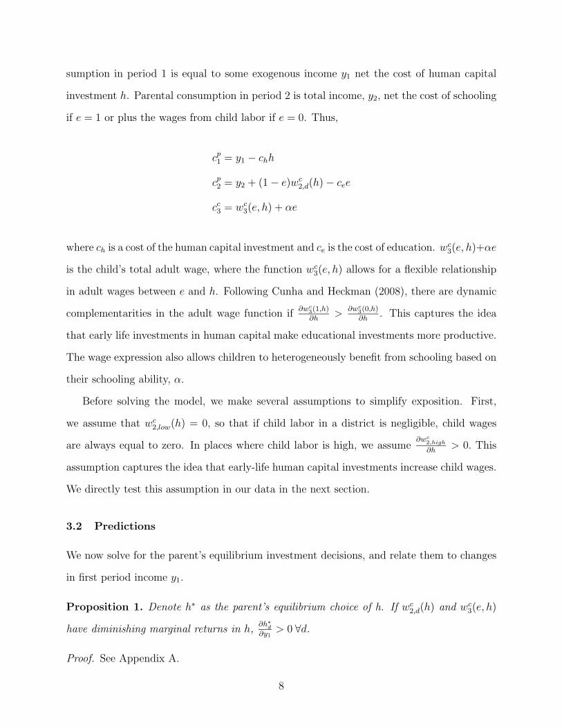

Proof See Appendix A
This proposition indicates that a positive income shock increases education (and adult
wages) more in low child labor districts than high child labor districts as long as the fact
that increased returns to the parent from child labor dominate two other second order
effects with ambiguous directions This is captured by the assumptionf(αlowast
high(hlowasthigh(y1)))
f(αlowastlow(hlowast
low(y1)))lt Φ4
The effect we expect to dominate is that an increase in h increases the relative returns to
education more in low child labor areas because in high child labor areas increasing h also
increases the outside option wc2d The additional ambiguous effects come from the fact that
(1) the density of children on the margin of being educated is different in high and low child
labor regions since enrollment rates are different and (2) the derivative of adult wages with
respect to early childhood investment may be different in high and low child labor regions
if underlying investment in h is different in these regions If underlying early-life human
capital investment rates are similar and the densities of the distribution at αlowastd(hd(y1)) are
similar across these regions these additional effects will be small5
Figure 3 illustrates the intuition for proposition 3a In both high and low child labor
districts the increase in y1 increases the relative returns to schooling causing αlowastd(h
lowastd)) to
fall But αlowastlow falls more than αlowast
high because the relative returns to schooling increase more in
low child labor districts The share of children whose educational outcomes are changed is
captured by the gray areas which integrate over the ability distribution from the old to the
new values of αlowastlow and αlowast
high Even though the density at the cut-off is different in high and
low child labor districts as long as it is not too much greater in high child labor districts more
children will be affected in low child labor districts where the integral is taken over a larger
set of values of α While proposition 3a shows that the effects of early-investment on the
4Φ =
partwc3(hlowast
low1)
party1minus
partwc3(0hlowast
low)
party1Ucprime(wc
3(0hlowastlow))
Ucprime(wc3(1hlowast
low)+αlowast
low)
partwc3(1hlowast
high)
party1minus
uprime(y2+wc2high
(hlowasthigh
))partwc
2d(hlowast
high)
party1+δ
partwc3(0hlowast
high)
party1Ucprime(wc
3(hlowasthigh
0))
δUcprime(wc3(1hlowast
high)+αlowast
high)
5The assumption thatf(αlowast
high(h(y1)))
f(αlowastlow(h(y1)))
lt Φ bounds how much greater the density at αlowastlow can be relatively
to the density at αlowasthigh That is if the density at αlowast
high is sufficiently high it can lead the response to shocksto be greater in high child labor places even though the change in the ability cut-off is smaller
10
returns to child labor can attenuate the positive effects of early-life investment on schooling
the next proposition shows that in extreme cases early-life investment can negatively affect
schooling
Proposition 3b Ifpartwc
2high(hlowast(y1))
parthis sufficiently great
partλhigh(y1)
party1lt 0
Proof See Appendix A
Proposition 3b shows that when the effect on parental utility of the increase in child
wages due to an increase in y1 is sufficiently large in high child labor places it outweighs
the effect of the increase in the returns to education (weighted by the parentsrsquo altruism and
discount rate) Then positive income shocks that increase early life investments can lead to
reduced education potentially translating into reduced wages later in life
4 Empirical Strategy and Results
Our model predicts that children with different initial levels of human capital will make
different choices to invest in schooling and that these choices can depend on the economic
environment To identify these effects we need variation in both the initial stock of human
capital and the labor market for children We will address these issues step-by-step First
in Section 41 we will show that rainfall shocks experienced early in life provide a plausibly
exogenous shock to the initial stock of human capital consistent with previous work (Maccini
and Yang 2009 Shah and Steinberg 2017) In Section 42 we show that these differences
in human capital affect child wages and thus their opportunity cost of education Secondly
in Section 43 we show that these differences in the initial stock of human capital cause
differential investment in education during childhood Third in Section 43 we show that
these responses to human capital stock differ based on the prevalence of child labor in the
districtmdashin places with low child labor children with high initial stocks of human capital
are significantly more likely to be in school during childhood and in places with the highest
child labor children are less likely to be in school and more likely to be working This is
11
consistent with both dynamic complementarities in the human capital production function
and a return to human capital in the market for child labor Lastly in Section 44 we use
crop shares as a more exogenous source of variation in child labor and find similar results
41 Variation in Early-Life Human Capital
To test the implications of the model we use early life rainfall shocks as a proxy for shocks
to early-life human capital The existing literature provides a strong argument for this rela-
tionship The argument is as follows positive rainfall shocks increase yield which increases
parental wages as shown by Jayachandran (2006) and Kaur (forthcoming) Intuitively and
as we also demonstrate in Prediction 1 of our model higher parental wages lead to higher
early-life investment (Maccini and Yang 2009 and Shah and Steinberg 2017) This could
take the form of increased nutrition for pregnant or breastfeeding mothers increased medical
care during infancy more parental time spent fostering development etc
Our data are consistent with these hypotheses As Appendix Table A1 shows positive
rainfall shocks increase yield Here a rainfall shock is coded as 1 if rain is greater than
the 80th percentile of the distribution from 1975 to 2008 minus1 if it is less than the 20th
percentile and 0 otherwise following Jayachandran (2006) Furthermore we replicate the
positive relationship between rainfall and wages found in the literature in Appendix Table
A2
We next aggregate rainfall shocks into a single child-level measure by taking the sum
across the three shocks in-utero age 1 and age 2 Tables 2 and 3 also confirm that early-life
shocks affect human capital in our data showing that children who experience shocks in
utero in their first year and in their second year have higher height and weight in the IHDS
(Table 2) and better test scores in the ASER (Table 3) These findings confirm Prediction 1
from the model and show that rainfall shocks are a relevant instrument for early-life human
capital investment
12
42 Early Human Capital Investments Affect Child Wages
We next turn to the key assumption of our model that early-life human capital investments
affect the opportunity cost of schooling by increasing child wages To test whether this is
the case we first use the IHDS to regress child wages on human capital measures with the
following specification
yidta = αa + β1human capidta + ΓXi + 983171idta
where i denotes a child a denotes age t denotes the survey round d denotes a district αa is
an age fixed effect and Xi is the set of controls consisting of gender and district fixed effects
human capi is our human capital measure which may be height weight or lagged math
scores Thus β1 is our coefficient of interest and we expect it to be positive We restrict
our sample to individuals aged 0ndash17 and cluster our standard errors at the district-level
Since our proxies for human capital are likely endogenous we next instrument for height
using our child-level aggregate rainfall shock measure Our first stage regression is then
human capidta = αa + λ1ELRdta +ΨXi + υidta
where ELRiat is the aggregate rainfall measure
Table 2 reports the results of these regressions In both the OLS and the IV we find
a positive relationship between child wages and measures of human capital supporting the
key assumption of the model that human capital investments also affect the outside option
43 Early-Life Investment and Schooling
We now turn to testing the key prediction of our model Based on Prediction 2 we expect
that if there are dynamic complementarities in districts with low child labor early life shocks
will increase educational investment In districts with high child labor this effect will be
13
attenuated (Proposition 3a) and may even be reversed (Proposition 3b) so that early-life
shocks decrease human capital investment
We first show graphical evidence that this is the case in Figures 4 and 5 Figure 4 shows
the effect of an early life rainfall shock on school attendance for children under 17 separately
by the district quintile of average child labor at baseline In places with low baseline child
labor positive early rainfall shocks increase school enrollment later in childhood However
as child labor increases this effect attenuates and in the districts in the highest quintile of
child labor the effect is reversed so that children with positive early life shocks are less likely
to be in school Figure 5 shows the opposite pattern for childrenrsquos work in low child-labor
districts children with positive shocks to human capital are less likely to be working but in
high child-labor districts they are significantly more likely to be working
To test whether this is the case we estimate the following regression
yidta = αa + β1ELRdta + β2ELRdta times CLd + γd + δt + 983171idta (1)
where yidta now consists of measures of working or being enrolled in school CLd is a measure
of the child labor in the district (either the percent of children engaged in child labor in the
NSS or an indicator variable for the percent being over a cut-off value) γd is a district fixed
effect and δt is a survey year fixed effect The remaining variables and subscripts are defined
as before
From Prediction 2 we expect β1 to be positive if there are dynamic complementarities
Prediction 3a predicts that β2 lt 0 indicating that the increase in child wages due to early-
life human capital investments reduces the positive effect of early-life human capital on
investment Prediction 3 suggests that cases may exist where β1 + β2 lt 0 indicating that
the effect of early-life human capital investment on child wages dominates the effect on the
returns to education
Table 5 reports the results of these regressions In Panel A we report estimates for the
14
effect of early life rain on whether a childrsquos primary activity is attending school On average
children who experience one more positive rain shock early in life are about 03 percentage
points more likely to attend school each year As this is the estimated effect on enrollment
for the average year over the course of the 17 years of child life included in the sample this
would lead to a 0051 year increase in schooling However in districts with more child labor
this effect is attenuated In fact in the districts in the top quintile of child labor children
who experience more rainfall early in life are significantly less likely to attend school Each
year a child who receives one more positive rainfall shock is 07 ppt less likely to be enrolled
Aggregating up this is a 012 year decrease in a childrsquos schooling For comparison a large
primary school construction program in Indonesia increased male schooling by 012 years
(Duflo 2001) suggesting that these effects are meaningful
In Panel B of Table 5 we replace school with work as the childrsquos primary activity for
the outcome variable The effects are similar Children in low child labor districts reduce
the likelihood of reporting working by 03 ppt suggesting they work 005 fewer years as a
result of one additional year of positive rainfall early in life Children in high child labor
places are 09 ppt more likely to work implying that they spend 0153 more years working in
aggregate The similarly sized (but opposite) effects on working and education suggest that
the positive early-life shocks mainly affect children on the margin between work and school
One potential threat to the validity of these estimates is that baseline child labor levels
may be correlated with an omitted variable that causes early life shocks to have smaller
(or negative) effects on education for other reasons Two of the most intuitive candidate
omitted variables are income and school quality For income high child labor areas could be
poorer so parents are less able to complement positive early-life shocks with later educational
investments or complementarities between schooling and educational investment could be
smaller because fewer high skilled jobs are available Similarly areas with high child labor
could have lower school quality reducing the complementarity between early life human
capital and education and therefore reducing parentsrsquo incentives to invest in education To
15
account for income we calculate the average adult wage and share of those who work for
a wage for each district at baseline and include the interaction between these controls and
ELRdta in equation (1) To account for school quality we take the average literacy rate in
each district and the primary and secondary school completion rates and also include these
interactions with ELRdta Figures 6 and 7 report the total effect of an early life shock in a
top quintile child labor district (β1 + β2CLd) for these new specifications For both working
and attending school the results are qualitatively similar to those without the controls
Figures 8 and 9 further explore the distribution of the effects of early-life shocks on
education and child labor across age groups These figures are generated by interacting
ELRdta and ELRdtatimesCLd with age fixed effects in equation (1) We then report estimates of
the total effect of a positive shock on education and working by age for children in districts in
the top quintile for child labor Consistent with the intuition of the model children exposed
to more positive early life rainfall shocks are neither more likely to work nor drop out until
the early stages of adolescence If anything preadolescent children exposed to early life
rainfall shocks are more likely to remain in school even in high child labor districts
44 Crop Variation as a Proxy for Child Labor
The share of children working in a given district is itself an equilibrium outcome caused by
various attributes of the district and the people who live there While in the previous section
we do not find that our measures of poverty or schooling qualitatively change the patterns
it is possible that we are measuring the (potential) confounders with error and that they
cause the differences in the response of education to early life shocks rather than child labor
itself To address this we take advantage of the fact that some crops are easier for children
to work on than others given the nature of the tasks associated with planting weeding and
harvesting the crops In the NSS cotton and sugar are the two crops that have the highest
proportion of workers under 18 (around 15 of workers in each crop are children at the start
of our sample) This is consistent with other contexts cotton in particular is notorious as a
16
child labor crop because it is low to the ground and very lightweight (Levy 1985) Cotton
and sugar both require somewhat specialized growing conditions and thus grow in only 20
of districts in India
We use both the presence of any sugar or cotton crop and the percentage of acreage in
the district of each of these crops as a proxy for child labor In Table 6 we re-estimate
our results from Table 5 using this proxy in place of district averages for child labor These
results tell a very similar story On average children who experience better early life rain
are less likely to be working and more likely to be attending school However in places with
cotton and sugar these effects are reversed and children who experience higher early life
rain are less likely to be in school and more likely to be working
5 Conclusion
Interventions that increase early-childhood investment may be a powerful tool for increasing
educational attainment overall However such policies could have counter-intuitive effects in
low-income countries where child labor is common We provide new evidence that early-life
investments increase child wages increasing the attractiveness of child labor Furthermore
we document the fact that while early-life investments positively affect educational outcomes
in places where child labor is low consistent with the existence of dynamic complementarities
this effect is attenuated in places where child labor is high In the places where child labor
is the highest early life interventions may even reduce long-term educational outcomes
These results have important implications both for policy-makers interested in increasing
educational outcomes and for researchers interested in identifying the form of the human
capital production function For the latter our results suggest that researchers particularly
those working in low-income countries must take into account how child human capital
affects the opportunity cost of schooling as well as the benefits of schooling
17
References
Agostinelli Francesco and Matthew Wiswall ldquoEstimating the Technology of Childrenrsquos SkillFormationrdquo NBER Working Paper 2016
Atkin David ldquoEndogenous Skill Acquisition and Export Manufacturing in Mexicordquo AmericanEconomic Review forthcoming
Attanasio Orazio Costas Meghir and Emily Nix ldquoHuman capital development andparental investment in indiardquo Technical Report NBER Working Paper 2015
Bharadwaj Prashant Leah K Lakdawala and Nicholas Li ldquoPerverse consequences of wellintentioned regulation evidence from Indiarsquos child labor banrdquo NBER Working Paper No 196022013
Cascio Elizabeth U and Ayushi Narayan ldquoWho Needs a Fracking Education The Ed-ucational Response to Low-Skill Biased Technological Changerdquo 2015 NBER Working Paper21359
Charles Kerwin Kofi Erik Hurst and Matthew J Notowidigdo ldquoHousing Booms andBusts Labor Market Opportunities and College Attendancerdquo 2015 NBER Working Paper21587
Cunha Flavio and James Heckman ldquoThe Technology of Skill Formationrdquo American EconomicReview Papers and Proceedings May 2007 97 (2) 31ndash47
and James J Heckman ldquoFormulating Identifying and Estimating the Technology of Cog-nitive and Noncognitive Skill Formationrdquo Journal of Human Resources 2008 43 (4) 738ndash82
Duflo Esther ldquoSchooling and Labor Market Consequences of School Construction in IndonesiaEvidence from an Unusual Policy Experimentrdquo The American Economic Review 2001 91 (4)795
Gilraine Mike Working Paper 2017
Jayachandran Seema ldquoSelling Labor Low Wage Responses to Productivity Shocks in Devel-oping Countriesrdquo Journal of Political Economy 2006 114 (3)
Johnson Rucker C and C Kirabo Jackson ldquoReducing Inequality Through Dynamic Comple-mentarity Evidence from Head Start and Public School Spendingrdquo Technical Report NBERWorking Paper 2017
Kaur Supreet ldquoNominal Wage Rigidity in Village Labor Marketsrdquo American Economic Reviewforthcoming
Knudsen Eric I James J Heckman Judy L Cameron and Jack P Shonkoff ldquoEconomicneurobiological and behavioral perspectives on building America s future workforcerdquo Proceedingsof the National Academy of Sciences 2006 103 (27) 10155ndash10162
Levy Victor ldquoCropping pattern mechanization child labor and fertility behavior in a farmingeconomy Rural Egyptrdquo Economic Development and Cultural Change 1985 33 (4) 777ndash791
18
Maccini Sharon and Dean Yang ldquoUnder the Weather Health Schooling and EconomicConsequences of Early-Life Rainfallrdquo American Economic Review June 2009 99 (3) 1006ndash26
Malamud Ofer Cristian Pop-Eleches and Miguel Urquiola ldquoInteractions Between Familyand School Environments Evidence on Dynamic Complementaritiesrdquo Technical Report NBERWorking Paper 2016
Shah Manisha and Bryce Millett Steinberg ldquoDrought of Opportunities Contemporaneousand Long Term Impacts of Rainfall Shocks on Human Capitalrdquo Journal of Political EconomyApril 2017 25 (2)
and ldquoWorkfare and Human Capital Investment Evidence from Indiardquo 2018 WIDERWorking Paper 21543
19
Figures
Figure 1 Distribution of Child Labor by District in the Indian NSS
Source NSS Round 57 (1999-2000)Notes This Figure shows the average level of child labor in each district where child labor is measured as the fraction ofindividuals age 0-17 who report their primary activity as working which includes wagesalary work work on a home enterprise(such as a farm or small business) or domestic work at home
20
Figure 2 The Educational Decision in the Model
Figure 3 Illustration of Proposition 3a
21
Figure 4 Effect of Early Life Rain on School Enrollment by Child Labor Prevalence
Source NSS Rounds 60-64 (1999-2008)Notes This Figure shows coefficients from a regression of early life rainfall shocks on school attendance separately for districtsin each quintile of average child labor The outcome variable is as dummy equal to one if a child reports attending school ashisher primary activity and zero if they report another primary activity The regressions contain fixed effects for district childage and child sex 95 confidence intervals clustered at the district level are shown in brackets
Figure 5 Effect of Early Life Rain on Working by Child Labor Prevalence
Source NSS Rounds 60-64 (1999-2008)Notes This Figure shows coefficients from a regression of early life rainfall shocks on child work separately for districts in eachquintile of average child labor The outcome variable is as dummy equal to one if a child reports working as hisher primaryactivity which includes wagesalary work work on a home enterprise (such as a farm or small business) or domestic work athome and zero if they report another primary activity The regressions contain fixed effects for district child age and childsex 95 confidence intervals clustered at the district level are shown in brackets
22
Figure 6 Effect of Early Life Rain on School Enrollment Controlling for additional DistrictCharacteristics
Source NSS Rounds 60-64 (1999-2008)Notes This Figure shows coefficients from a regression of early life rainfall shocks on school attendance with additional controlsThe outcome variable is as dummy equal to one if a child reports attending school as hisher primary activity and zero if theyreport another primary activity Additional controls include schooling controls (district average literacy rate primary schoolcompletion rate and secondary school completion rate) interacted with early life shock and income controls (share of adultswho work for a wage and average wage) interacted with early life shocks The regressions contain fixed effects for district childage and child sex 95 confidence intervals clustered at the district level are shown in brackets
23
Figure 7 Effect of Early Life Rain on Working Controlling for additional District Charac-teristics
Source NSS Rounds 60-64 (1999-2008)Notes This Figure shows coefficients from a regression of early life rainfall shocks on child work with additional controls Theoutcome variable is as dummy equal to one if a child reports working as hisher primary activity which includes wagesalarywork work on a home enterprise (such as a farm or small business) or domestic work at home and zero if they report anotherprimary activity Additional controls include schooling controls (district average literacy rate primary school completion rateand secondary school completion rate) interacted with early life shock and income controls (share of adults who work for awage and average wage) interacted with early life shocks The regressions contain fixed effects for district child age and childsex 95 confidence intervals clustered at the district level are shown in brackets
24
Figure 8 Effect of Early Life Rain on School Enrollment by Age
Source NSS Rounds 60-64 (1999-2008)Notes This Figure shows coefficients from a regression of early life rainfall shocks on child work separately for each age Theoutcome variable is as dummy equal to one if a child reports attending school as hisher primary activity and zero if they reportanother primary activity The regressions contain fixed effects for district and child sex 95 confidence intervals clustered atthe district level are shown in brackets
Figure 9 Effect of Early Life Rain on Working by Age
Source NSS Rounds 60-64 (1999-2008)Notes This Figure shows coefficients from a regression of early life rainfall shocks on child work separately for each age Theoutcome variable is as dummy equal to one if a child reports working as hisher primary activity which includes wagesalarywork work on a home enterprise (such as a farm or small business) or domestic work at home and zero if they report anotherprimary activity The regressions contain fixed effects for district and child sex 95 confidence intervals clustered at thedistrict level are shown in brackets
25
Tables
Table 1 Data SourcesData Source Type Years Variables UsedNational Sample Survey (NSS) Repeated 20002004-2008 avg child labor
Cross-Section primary activityAnnual Status of Repeated 2005-2009 drop-outsEducation Report (ASER) Cross-SectionIndia Human Development HH Panel 2005 and child wagesSurvey (IHDS) 2012 anthropometrics
math scoresWorld Bank India District 1975-1987 crop yieldsAgriculture and Climate PanelData SetUniversity of Delaware District 1970-2008 rain shocksGridded Rainfall Data Panel
26
Table 2 Relationship Between Child Human Capital and Wages in the IHDS
Dependent Variable Log Child Wages
Height 0077 0089(0021)lowastlowastlowast (0038)lowastlowast
Weight 0065 0023(0023)lowastlowastlowast (0044)
Lagged Math Scores 0228 0134(0258) (0309)
Ages 0-17 0-17 15-17 15-17Mean DV 145 145 154 154Observations 1302 1296 880 695
Source Data on wages height and weight come from the IHDS II (2012-13) and lagged math scores from IHDS I (2005-6)Notes This table shows coefficients from an OLS regression of the natural logarithm of wages on measures of human capitalHeight is measured in centimeters and weight is measured in kilograms Lagged math scores range from 0-4 and are availableonly for those adolescents in 2012-13 who were age 8-11 in 2005-6 and able to be matched to IHDS-I All regressions includegender and age fixed effects Standard errors clustered at the district level are reported in parentheses indicates significanceat 1 level at 5 level at 10 level
Table 3 Effect of Early Life Rain on Size and Test Scores
Dependent Variable Height Weight Math Math Word ReadScore Problem Score
Rainshock in Utero 293 115 014 0049 017(0874)lowastlowastlowast (071) (0044)lowastlowastlowast (0042) (0043)lowastlowastlowast
Rainshock in Year of Birth 2752 0193 011 0078 011(1015)lowastlowastlowast (0701) (0045)lowastlowast (0044)lowast (0045)lowastlowast
Rainshock in Year After Birth 215 -0497 014 018 016(0881)lowastlowast (065) (0043)lowastlowastlowast (0046)lowastlowastlowast (0043)lowastlowastlowast
Ages 5-17 5-17 5-16 5-16 5-16Mean DV 12597 2755 263 126 272Observations 36953 37409 2351596 844619 2363553
Source Data on height and weight come from the IHDS II (2012-13) data on test scores from ASER (2005-9) and data onrainfall from the University of DelawareNotes This table shows coefficients from an OLS regression of measures of human capital on early life rain Height is measuredin centimeters and weight is measured in kilograms Math and reading test scores range from 0-4 and math word problemranges from 0-2 Rainshock is equal to one if yearly rainfall is above the 80th percentile for the district negative one if rainfallis below the 20th percentile and zero otherwise All regressions contain fixed effects for sex age year and district Standarderrors clustered at the district level are reported in parentheses indicates significance at 1 level at 5 level at 10level Data IHDS 2012-13 amp University of DelawareAll regressions contain district year gender and age FE
27
Table 4 Effect of Early Life Rain on Work and Wages
(1) (2) (3)ln(wages)
Full Sample Boys GirlsEarly Life Rain 0020 0025 -0005
(0010) (0013) (0016)Mean Outcome 534 544 513Number Districts 492 464 289Number Observations 6858 4540 2208
Source NSS Rounds 60-64 (1999-2008)Notes This table shows coefficients from a regression of the natural logarithm of wages on early life rain Early life rain isthe sum of rainshock in the first three years after conception (in utero-age 1) where rainshock is equal to one if yearly rainfallis above the 80th percentile for the district negative one if rainfall is below the 20th percentile and zero otherwise Wagesare only measured for children who report positive wage earnings All regressions contain fixed effects for sex age year anddistrict Standard errors clustered at the district level are reported in parentheses indicates significance at 1 level at 5 level at 10 level
28
Table 5 Effect of Early Life Shocks on School and Work in High Child Labor Districts
Panel A School Attendance
(1) (2) (3) (4)Attends School
Early Life Rain 0003 0008 0006 0005(0001) (0002) (0002) (0001)
Early Life Rain times -0120Child Labor (0025)
Early Life Rain times -0007(Above Median) Child Labor (0002)
Early Life Rain times -0012(Top Quintile) Child Labor (0003)
Mean Outcome 602 602 602 602P Value for Total Effect = 0 001 522 012Number Districts 552 552 552 552Number Observations 386923 386923 386923 386923
Panel B Working
(1) (2) (3) (4)Primary Activity Works
Early Life Rain -0001 -0007 -0005 -0003(0001) (0001) (0001) (0001)
Early Life Rain times 0129Child Labor (0021)
Early Life Rain times 0009(Above Median) Child Labor (0002)
Early Life Rain times 0012(Top Quintile) Child Labor (0002)
Mean Outcome 04 04 04 04P Value for Total Effect = 0 004 002 0Number Districts 552 552 552 552Number Observations 406179 406179 406179 406179
Source NSS Rounds 60-64 (1999-2008) and data on rainfall from the University of DelawareNotes This table shows coefficients from a regression of primary activity on early life rain interacted with measures of childlabor prevalence by district In Panel A the outcome variable is ldquoattends schoolrdquo which is equal to one if a child reports theirprimary activity as attending school and zero if they report something else In Panel B the outcome variable to ldquoworksrdquo whichis equal to one if a child reports any productive activity as his primary activity (such as wagesalary work home enterpriseor domestic work) and zero if he reports something else Early life rain is the sum of rainshock in the first three years afterconception (in utero-age 1) where rainshock is equal to one if yearly rainfall is above the 80th percentile for the district negativeone if rainfall is below the 20th percentile and zero otherwise The measure of child labor is the percent of children age 0-17 inthe district in NSS round 57 (1999-2000) who report working as their primary activity All regressions contain fixed effects forsex age year and district Standard errors clustered at the district level are reported in parentheses indicates significanceat 1 level at 5 level at 10 level
29
Table 6 Effect of Early Life Shocks on School and Work in CottonSugar Districts
(1) (2) (3) (4) (5) (6)Primary Activity Works Attends School
Early Life Rain -0001 -0006 -0002 0003 0007 0004(0001) (0002) (0001) (0001) (0003) (0001)
Early Life Rain times SugarCotton 0009 -0007(0004) (0005)
Early Life Rain times Has SugarCotton 0004 -0008(0002) (0003)
Mean Outcome 04 04 04 603 603 603P Value for Total Effect = 0 486 067 026 165Number Districts 564 564 564 564 564 564Number Observations 409793 409793 409793 390319 390319 390319
Source NSS Rounds 60-64 (1999-2008) and data on rainfall from the University of DelawareNotes This table shows coefficients from a regression of primary activity on early life rain interacted with measures of childlabor prevalence by district In Panel A the outcome variable is ldquoattends schoolrdquo which is equal to one if a child reports theirprimary activity as attending school and zero if they report something else In Panel B the outcome variable to ldquoworksrdquo whichis equal to one if a child reports any productive activity as his primary activity (such as wagesalary work home enterpriseor domestic work) and zero if he reports something else Early life rain is the sum of rainshock in the first three years afterconception (in utero-age 1) where rainshock is equal to one if yearly rainfall is above the 80th percentile for the district negativeone if rainfall is below the 20th percentile and zero otherwise The measure of cottonsugar is the percent of agriculture thatis concentrated in these two crops in the district in NSS round 57 (1999-2000) All regressions contain fixed effects for sex ageyear and district Standard errors clustered at the district level are reported in parentheses indicates significance at 1level at 5 level at 10 level
30
Appendix Tables
Table A1 High Rain Increases Crop YieldsDependent Variable
Rice Jowar Maize Bajra
Rain Shock Current Year 11 03 02 04(02)lowastlowastlowast (009)lowastlowastlowast (005)lowastlowastlowast (009)lowastlowastlowast
Year fixed effects Y Y Y YDistrict fixed effects Y Y Y YControls Y Y Y YObservations 2987 2674 2825 2297Mean Dependent Variable 151 589 282 291
Source Agricultural yields from the World Bank India Agriculture and Climate Data Set (1975-1987) and data on rainfall fromthe University of DelawareNotes This table shows coefficients from a regression of crop yields on currents rainshock where rainshock is equal to oneif yearly rainfall is above the 80th percentile for the district negative one if rainfall is below the 20th percentile and zerootherwise All regressions contain fixed effects for year and district and controls for agricultural inputs Standard errorsclustered at the district level are reported in parentheses indicates significance at 1 level at 5 level at 10 level
Table A2 High Rain Increases WagesDependent Variable log(wages)Rain Shock Current Year 02
(009)lowast
Year fixed effects YDistrict fixed effects YObservations 167017Mean Dependent Variable 585
Source NSS Rounds 60-64 (1999-2008) and data on rainfall from the University of DelawareNotes This table shows coefficients from a regression of the natural logarithm of adult wages (age 18-64) on current rainshockwhere rainshock is equal to one if yearly rainfall is above the 80th percentile for the district negative one if rainfall is belowthe 20th percentile and zero otherwise Wages are only measured for adults who report positive wage earnings All regressionscontain fixed effects for year and district and controls for agricultural inputs Standard errors clustered at the district levelare reported in parentheses indicates significance at 1 level at 5 level at 10 level
31
Appendix A
Proof of Proposition 1
Define V = Emaxe u(y2minuscee+wc2d(h)(1minuse))+δ(U c(wc
3(e h))+αe) where the expectation
is taken over realizations of α Then in period 1 the parent solves
maxh
u(y1 minus chh) + βV (h)
where β is the discount rate hlowast must satisfy
F = minuschuprime(y1 minus chh
lowast) + βpartV (hlowast)
parth= 0
To sign parthlowast
party1 apply the implicit function theorem to F By the implicit function theorem
parthlowast
party1= minusFy1
Fhlowast Then
Fhlowast = c2huprimeprime(y1 minus chh
lowast) + βpart2V (hlowast)
parth2
where c2huprimeprime(y1 minus chh
lowast) lt 0 To sign part2V (hlowast)parth2 observe that
part2V (hlowast)
parth2=E
983059uprimeprime(y2 minus cee
lowast + wc2d(h)(1minus elowast))
983059wc2d(h)
parth
9830602
+ uprime(y2 minus ceelowast + wc
2d(h)(1minus elowast))part2wc
2d(h)
parth2
+ δ983059U cprimeprime(wc
3(h elowast) + αelowast)
983059partwc3(e
lowast h)
parth
9830602
+ (U cprime(wc3(e
lowast h) + αelowast)part2wc
3(elowast h)
parth2
983060983060
where elowast is the equilibrium choice of e This expression is lt 0 ifpart2wc
3(h)
parth2 le 0 andpart2wc
2(h)
parth2 le 0
Therefore Fhlowast lt 0 Observe that
Fy1 = minuschuprimeprime(y1 minus chh
lowast) gt 0
Then it follows from the implicit function theorem that parthlowast
party1gt 0
32
Proof of Proposition 2 Given h a child drops out if Up2 (0 h) ge Up
2 (1 h) Substituting
in the values for consumption this expression can be rewritten as
u(y2 + wc2d(h))minus u(y2 minus ce) ge δ(U c(wc
3(h 1) + α)minus U c(wc3(h 0)))
The derivative of the LHS with respect to y1 is partLHSparty1
= uprime(y2 + wc2(h))
partwc2d(h
lowast)
parthparthlowast
party1 which is
equal to 0 in low child labor places by assumption The derivative of the RHS is partRHSparty1
=
δ983059U cprime(wc
3(hlowast 1) + α)
part2wc3(h1)
parthparthlowast
party1minus U cprime(wc
3(h 0))partwc
3(h0)
parthparthlowast
party1
983060 From diminishing marginal re-
turns U cprime(wc3(h 1) + α) lt U cprime(wc
3(h 0)) so for the RHS to be increasing we need that
partwc3(h1)
parthgt
partwc3(h0)
parth This expression implies that for an early life shock to increase education
rates in low child labor areas there are dynamic complementarities between e and h
Before proof Proposition 3a we define Assumption A1
Assumption A1
Φ gtf(αlowast
high(h(y1)))
f(αlowastlow(h(y1)))
where
Φ =
partwc3(h
lowastlow1)
party1minus
partwc3(0h
lowastlow)
party1Ucprime(wc
3(0hlowastlow))
Ucprime(wc3(1h
lowastlow)+αlowast
low)
partwc3(1h
lowasthigh)
party1minus
uprime(y2+wc2high(h
lowasthigh))
partwc2d
(hlowasthigh
)
party1+δ
partwc3(0h
lowasthigh
)
party1Ucprime(wc
3(hlowasthigh0))
δUcprime(wc3(1h
lowasthigh)+αlowast
high)
Proof of Proposition 3a
Observe that λd(hlowast(y1)) = 1minusF (αlowast
d(hlowastd(y1))) Therefore
partλd(hlowastd(y1))
party1= minusf(αlowast
d(hlowastd(y1))
partαlowastd(h
lowastd(y1))
party1
To solve forpartαlowast
d(hlowastd(y1))
party1 note that αlowast
d(hlowastd(y1)) is characterized by Up
2 (0 hlowastd(y1)) = Up
2 (1 hlowastd(y1))
which can be rewritten as
u(y2 + wc2d(h
lowastd))minus u(y2 minus cee)minus δU c(wc
3(1 hlowastd) + αlowast
d) + δU c(wc3(0 h
lowastd)) = 0
33
Applying the implicit function theorem to this expression we arrive at an expression forpartαlowast
d
party1
partαlowastd
party1= minuspartwc
3(1 hlowastd)
party1+
uprime(y2 + wc2d(h
lowastd))
partwc2d
party1+ δ
partwc3(0h
lowastd)
party1U cprime(wc
3(0 hlowastd))
δU cprime(wc3(1 h
lowastd) + αlowast
d)
Substituting this expression into partλd(hlowast(y1))
party1= minusf(αlowast
d(hlowastd(y1))
partαlowastd(h
lowast(y1))
party1 we find that
partλlow(hlowastlow(y1))
party1=
983075partwc
3(1 hlowastlow)
party1minus
partwc3(0h
lowastlow)
party1U cprime(wc
3(hlowastlow 0))
U cprime(wc3(1 h
lowastlow) + αlowast
low)
983076f(αlowast
low)
partλhigh(hlowasthigh(y1))
party1=
983091
983107partwc3(1 h
lowasthigh)
party1minus
uprime(y2 + wc2high(h
lowasthigh))
partwc2d(h
lowasthigh)
party1+ δ
partwc3(0h
lowasthigh)
party1U cprime(wc
3(hlowasthigh 0))
δU cprime(wc3(1 h
lowasthigh) + αlowast
high)
983092
983108
times f(αlowasthigh)
Thus partλlow(hlowast(y1))party1
gtpartλhigh(h
lowast(y1))
party1under Assumption A1 To provide intuition for when
Assumption A1 is satisfied when hlowastd and αlowast
d are sufficiently similar across the two types
of districts Φ gt 1 This is because the additional term in the denominator uprime(y2 +
wc2high(h
lowasthigh))
partwc2d(h
lowasthigh)
party1gt 0 indicating that the denominator is smaller than the numer-
ator If αlowastlow and αlowast
high are sufficiently similarf(αlowast
high(h(y1)))
f(αlowastlow(h(y1)))
asymp 1 and Assumption A1 will be
satisfied
Proof of Prediction 3b Recall thatpartλhigh(h
lowasthigh(y1))
party1= minusf(αlowast
high(hlowasthigh(y1))
partαlowasthigh(h
lowasthigh(y1))
party1
where f(αlowasthigh) gt 0 and
partαlowasthigh
party1= minus
partwc3(1 h
lowasthigh)
party1+
uprime(y2 + wc2high(h
lowasthigh))
partwc2high
party1+ δ
partwc3(0h
lowasthigh)
party1uprime(wc
3(0 hlowasthigh))
δU cprime(wc3(1 h
lowasthigh) + αlowast
high)
Thenpartλhigh(h
lowasthigh(y1))
party1lt 0 if
partαlowasthigh
party1gt 0 Rearranging
partαlowasthigh
party1gt 0 shows that this satisfied if
δ
983091
983107partwc
3(1hlowasthigh)
party1U cprime(wc
3(1 hlowasthigh) + αlowast
high)minuspartwc
3(0hlowasthigh)
party1U cprime(wc
3(0 hlowasthigh))
uprime(y2 + wc2(h
lowasthigh))
983092
983108983061parth
party1
983062minus1
ltpartwc
2(hlowasthigh)
parth
34
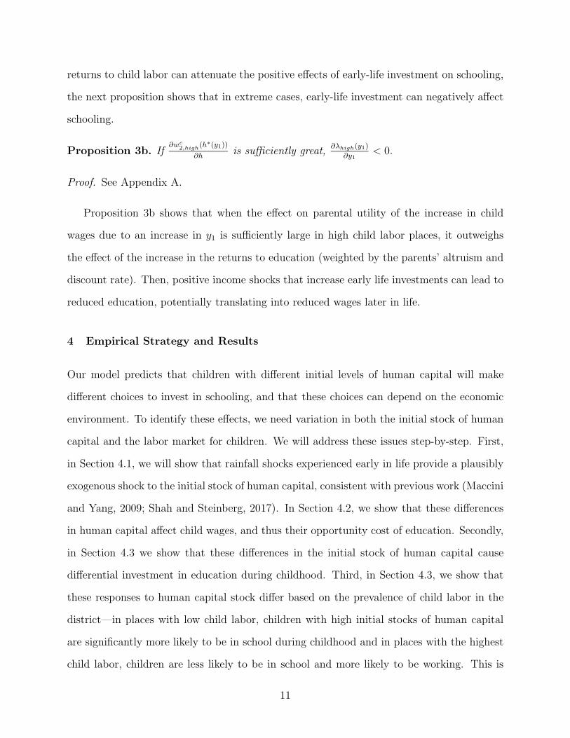
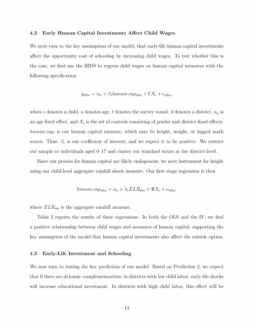
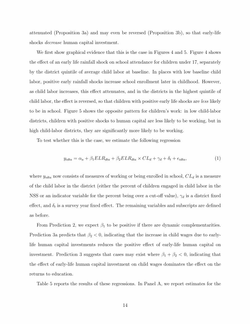
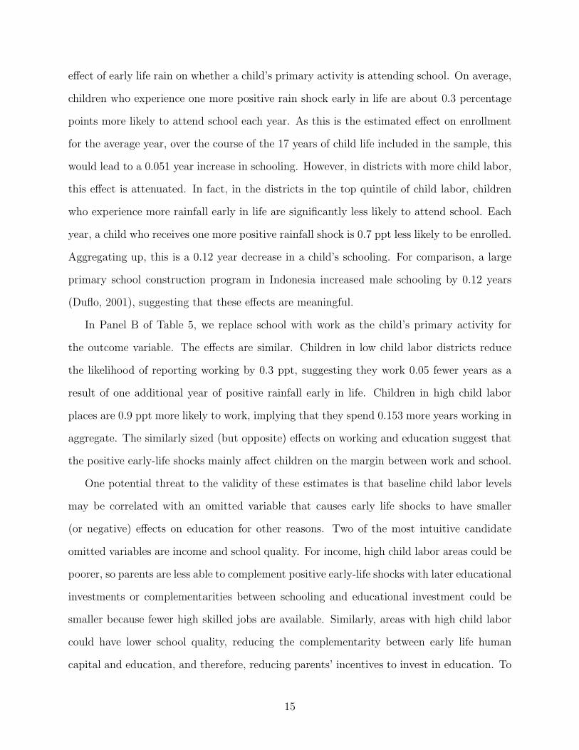
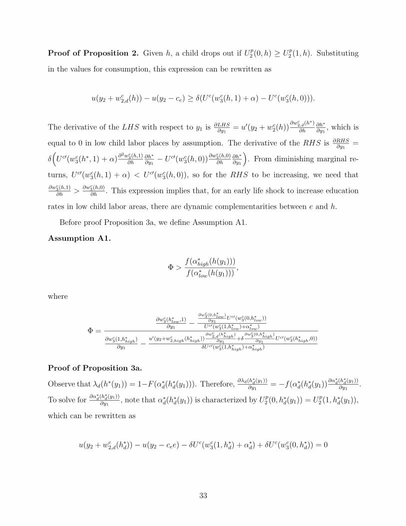
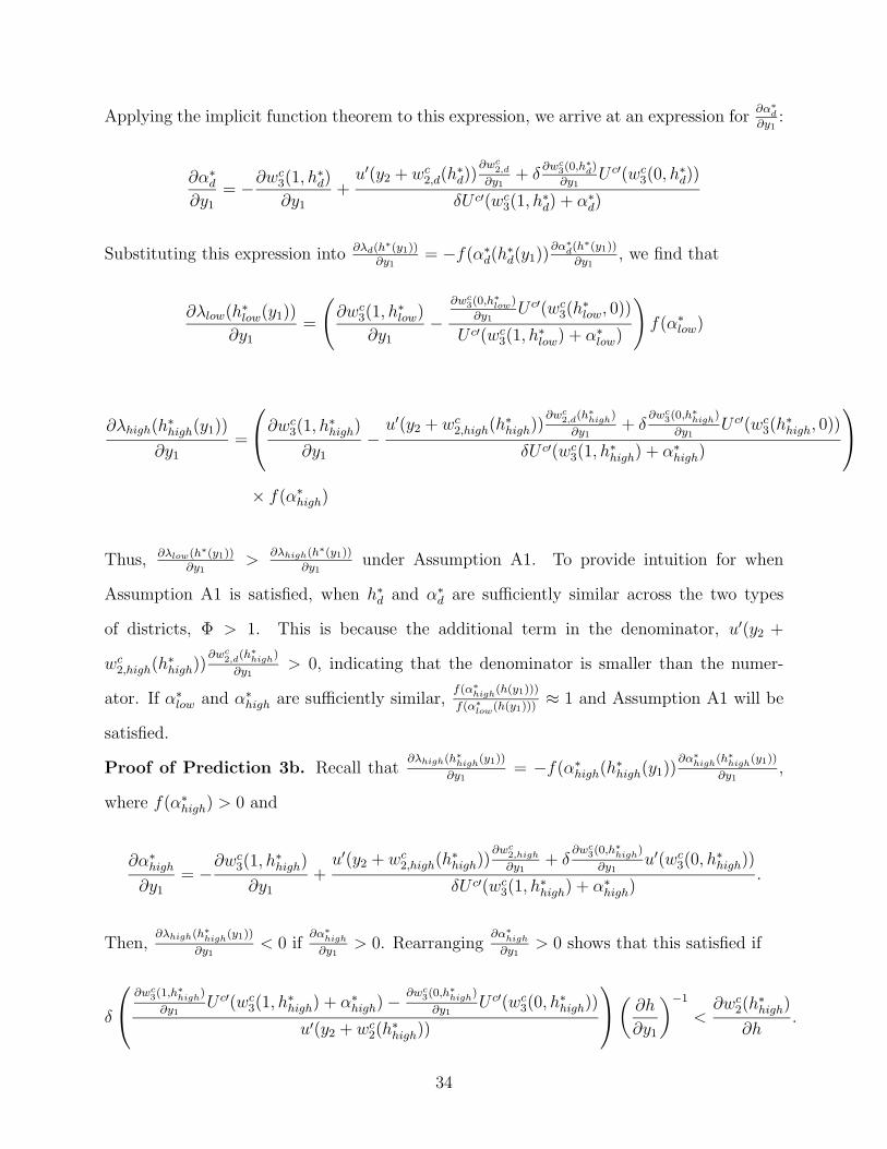