brain activity mapping from meg data via a hierarchical...
TRANSCRIPT

Brain activity mapping from MEG data via a hierarchical
Bayesian algorithm with automatic depth weighting
Daniela Calvetti∗, Annalisa Pascarella†, Francesca Pitolli‡,Erkki Somersalo§, Barbara Vantaggi¶
June, 2018
Abstract
A recently proposed Iterated Alternating Sequential (IAS) MEG inverse solver algorithm,based on the coupling of a hierarchical Bayesian model with computationally efficient Krylovsubspace linear solver, has been shown to perform well for both superficial and deep brainsources. However, a systematic study of its ability to correctly identify active brain regionsis still missing. We propose novel statistical protocols to quantify the performance of MEGinverse solvers, focusing in particular on how their accuracy and precision at identifying activebrain regions. We use these protocols for a systematic study of the performance of the IASMEG inverse solver, comparing it with three standard inversion methods, wMNE, dSPM, andsLORETA. To avoid the bias of anecdotal tests towards a particular algorithm, the proposedprotocols are Monte Carlo sampling based, generating an ensemble of activity patches in eachbrain region identified in a given atlas. The performance in correctly identifying the activeareas is measured by how much, on average, the reconstructed activity is concentrated in thebrain region of the simulated active patch. The analysis is based on Bayes factors, interpretingthe estimated current activity as data for testing the hypothesis that the active brain region iscorrectly identified, vs. the hypothesis of any erroneous attribution. The methodology allowsthe presence of a single or several simultaneous activity regions, without assuming that thenumber of active regions is known. The testing protocols suggest that the IAS solver performswell with both with cortical and subcortical activity estimation.Keywords: MEG inverse problem; Activity map; Brain region; Bayes factor; Deep sources
1 Introduction
In the ongoing quest for understanding brain functions and connectivity, during specific tasksand in resting states, with the hope of finding a functional fingerprint of autism, pathologicaldepression or schizophrenia, the potential of MEG as a non-invasive and non-disturbing brainactivity mapping modality cannot be emphasized enough. The high temporal resolution of MEG
∗Case Western Reserve University, Department of Mathematics, Applied Mathematics and Statistics, 10900Euclid Avenue, Cleveland, OH 44106, e-mail: [email protected]†CNR - National Research Council, Istituto per le Applicazioni del Calcolo “Mauro Picone”, Via dei Taurini 19,
00185 Rome, Italy, e-mail: [email protected]‡University of Roma ”La Sapienza”, Department SBAI, Via A. Scarpa 16, 00161 Roma, Italy e-mail:
[email protected]§Case Western Reserve University, Department of Mathematics, Applied Mathematics and Statistics, 10900
Euclid Avenue, Cleveland, OH 44106, e-mail: [email protected]¶University of Roma ”La Sapienza”, Department SBAI, Via A. Scarpa 16, 00161 Roma, Italy, e-mail:
1
offers enormous possibilities for understanding the fine details of brain dynamics, however thereliable reconstruction of activity patterns in cortical and deep brain regions relies on the capabilityof the underlying inverse solver to correctly identify active brain areas. In this work we proposea comprehensive, statistically sound methodology to assess the performance of different inversesolvers, and demonstrate the viability of the approach by applying it to four different algorithms.
A fundamental difficulty in the solution of the MEG inverse problem (Hamalainen el al., 1993,Baillet et al., 2001, Brette el al., 2012) comes from the non-uniqueness of the solution and thehigh sensitivity of the problem to noise in the data. To address the non-uniqueness, it is necessaryto augment the data with additional information about the solution, which entails either theintroduction of regularization techniques in a deterministic setting, or the introduction of priormodels in the Bayesian framework. The sensitivity of the computed solution to noise, with lowsignal-to-noise ratio of data, in turn, requires a good understanding of the noise sources, whichin the Bayesian framework is related to a design of a reliable likelihood. These considerationshighlight the importance of being able to assess the reliability of a given inversion algorithm in themultitude of tasks it may be applied to, and to quantify the uncertainty in computed solutions.
In this article, we present a systematic study of the accuracy and precision of the IterativeAlternating Sequential (IAS) MEG inversion algorithm (Calvetti et al., 2009, 2015), which pairshierarchical Bayesian modeling with a computationally very efficient prior-based preconditionediterative linear solver. Numerous algorithms based on hierarchical Bayesian modeling have beensuggested in the literature, see, e.g., (Auranen et al., 2005, Calvetti et al., 2009, Henson el al., 2009,2010, Kiebel el al., 2008, Lucka et al., 2012, Lopez et al., 2014, Mattout et al., 2006, Nummenmaaet al., 2007,b, Owen et al., 2012, Sato et al., 2004, Stephan et al., 2009, Trujillo-Barreto et al.,2004, Wipf and Nagarajan, 2009, Wipf et al., 2010). A common feature of these methods is theuse of parameter-dependent prior models, the model parameters representing the second layer ofunknowns. A standard approach in hierarchical Bayesian modeling is to introduce a hyperpriormodel for the parameters, and to either marginalize, or model average, the parameters, or to esti-mate them by maximizing the evidence, see, e.g., Bernardo and Smith (2004) for general reference.A more time-consuming approach to the hierarchical modeling avoiding optimization techniques isto use Markov chain Monte Carlo (MCMC) methods.
The IAS MEG algorithm, too, is based on the use of hierarchical, conditionally Gaussian modelfor the prior. The hyperparameters are the variances of the elementary sources in the currentdensity model, and are adjusted by learning focality from data. To reduce the computational com-plexity of the problem, especially in case of high dimensionality of the MEG data, the algorithmapproximates the maximum of the posterior distribution instead of computing the posterior distri-bution itself. The iterative alternating sequential minimization procedure was shown to converge inCalvetti et al. (2015), where an easily implementable procedure for the estimation of the maximizerof the posterior with respect to both the unknown of primary interest and the hyperparameterswas proposed. The maximization algorithm uses a dynamically preconditioned Krylov subspaceiterative solver equipped with a stopping rule that monitors the fidelity of the solution to dataand stops the iteration before amplified noise components begin to degrade the computed solution.The solution of the regularized subproblem does not rely on a Tikhonov-regularized linear solver,but on a very fast converging preconditioned Conjugate Gradient Least Squares (CGLS) algo-rithm, which makes the solution depend non-linearly on the data (Calvetti et al., 2018). Moreover,the IAS MEG inverse method employs an anatomically justified prior: Based on the segmentedsubject-specific MRI image containing the information of the cortical surface orientation, for eachdipole there is a direction which is favored, but not forced, by the prior model. Similar ideas withdifferent implementation have been suggested in the literature, see. e.g. (Lin el al., 2006b).
Some of the appeal of standard MEG solvers such as MNE (Hamalainen MS and IlmoniemiRJ, 1984, Lin el al., 2006a) or LORETA (Pasqual-Marqui, 1999) is their simplicity of use, withminimal user intervention required, e.g., for setting parameters or controlling the optimization
2

process, which is not always the case with hierarchical models. One of the goals in developing theIAS algorithm was to have a robust and convergent method that depends on very few user-suppliedparameters with an intuitive meaning. In Calvetti et al. (2009), the connection between theconditionally Gaussian hierarchical models and several sparsity-promoting methods ( Gorodnitskyand Rao, 1997, Nagarajan et al., 2006, Uutela et al., 1999) was pointed out.
A novel contribution of this paper is to provide a physical interpretation of the hyperparam-eters and to establish a connection with sensitivity weighting. The IAS algorithm, as it wasrigorously shown in Calvetti et al. (2015), contains only one user-supplied parameter that controlsthe sparsity of the solution and, as pointed out in Section 2.2, the other hyperparameters can besemi-automatically set based on the information about the signal-to-noise ratio. This formulationprovides a proper Bayesian interpretation for the sensitivity weighting that is commonly used with,e.g., the Minimum Norm Estimate (MNE) and the Minimum Current Estimate (MCE) (Uutela etal., 1999) algorithms to overcome the propensity of the methods to favor superficial sources overdeep ones, thereby filling the gap between Bayesian modeling and traditional regularization.
The quest for MEG inverse solvers capable of identifying activities both on superficial cortex andin deeper brain regions continues to be of interest. In Attal et al. (2012), Attal and Schwartz (2013)the localization accuracy of subcortical generators was studied for three different algorithms: theweighted Minimum Norm Estimate (wMNE), dynamic Statistical Parametric Mapping (dSPM),and standardized Low Resolution Brain Electromagnetic Tomography (sLORETA). The procedurerelies on a realistic electrophysiological model of deep brain activity and compares the performanceof the three methods in recovering activity in the neocortex, hippocampus, amygdala and thalamus.In the present study the comparison is extended to include the IAS method using a model of thesubcortical regions that considers their surface envelopes, adding basal ganglia, brainstem andcerebellum to the list of brain regions, and introducing a statistically justified metric to evaluatethe performances of the different algorithms.
More specifically, our investigation addresses the following question: Given an atlas of anatomo-functional brain regions (BR), how well does the IAS method for the MEG inversion identify activeregions, and to what extent non-active regions will be correctly deemed as inactive ones? With aslight abuse of terminology, we may refer to the former question as sensitivity of the MEG inversesolver, and to the latter as specificity, elaborating on the reasons for this choice further below.In line with the Bayesian paradigm that IAS is based on, we investigate these questions usingstatistical tools. For this purpose we introduce an Activity Level Indicator (ALI), measuring themean activity level of each BR given a simulated patch activity in a selected BR, and computethe first and second order statistics of this indicator over a sample of random activation patchesin the selected BR. To assess the relative performance of IAS, we compare these statistics withthose of three other standard inversion methods, wMNE (Lin el al., 2006a), dSPM (Dale et al.,2000), and sLORETA (Pasqual-Marqui, 1999, Wagner et al., 2004), using the implementationsprovided in Brainstorm (Tadel et al., 2011). Furthermore, to test the relative performance of thefour methods, we observe that a common approach in the Bayesian methodology to test hypothesesor models is to use Bayes factors of probabilities of the data, given the competing hypotheses ormodels (Bernardo and Smith, 2004, Kass RE and Raftery AE, 1995). In the current setting, weinterpret the estimated activity as data, and test the probabilities of them under the competinghypotheses of having activity in the correct BR versus having it in another randomly chosen BR.We compare the specificity of the IAS algorithm to that of the other three standard solvers usingsimulated data under two different scenarios: when there is only one active patch in a cortical orsubcortical region, and when there are multiple (from two to six) active patches in cortical andsubcortical regions. In this way we can test not only the sensitivity and specificity of each inversesolver with respect to a single BR, but also their ability of recovering an activation pattern whenother regions disturb the identification. We conclude the computed experiments by comparing thereconstructions obtained by the four inverse solvers in an example starting from real data, where
3

the underlying activation pattern is not known exactly but is inferred from the protocol used forthe data collection.
2 Materials and Methods
We start by presenting a brief review of the Iterative Alternating Sequential (IAS) MEG inversesolver, described in detail in Calvetti et al. (2015). Subsequently, we introduce the computationaltools that will be used for testing the algorithm’s performance, focusing in particular on its capacityto identify active areas of interest from the MEG data and comparing it to three other mainstreamMEG inverse solvers.
To discretize the problem, we approximate the cortical surface, as well as the surface of thesubcortical structures, by a triangular mesh with n vertices, whose coordinates are denoted by vj .We associate to each vertex a unit length vector ~νj pointing in the direction normal to the localcortical/subcortical surface.
The forward model is of the form
b =
n∑
j=1
Mj~qj + ε, (1)
where b ∈ Rm is the observation vector representing the measured magnetic field components,Mj ∈ Rm×3 is the lead field matrix associated with the jth dipole located at vj , ~qj is the jth dipolemoment and ε ∈ Rm is additive observation noise. The lead field matrices take into account theconductivity structure of the head model. While changing the forward model does not affect theinversion algorithm, the results are to some extent sensitive to the model used (cf. Vorwerk el al.(2014)).
We model the noise term as a zero mean Gaussian random variable, ε ∼ N (0,Σ), whereΣ ∈ Rm×m is the covariance matrix. To model biological noise, the covariance needs to reflectthe cross correlations between the channels, as will be discussed below. Therefore, the likelihooddensity of b conditioned on ~q1, . . . , ~qn can be written as
π(b | ~q1, . . . , ~qn) ∝ exp
−1
2‖b−
n∑
j=1
Mj~qj‖2Σ
,
where ‖z‖2Σ = zTΣ−1z is the square of the Mahalanobis norm and “∝” stands for “proportionalup to a normalizing constant”. In our computer simulation a small exogenous noise component isadded to the biological noise.
2.1 The inverse solver: an overview
The IAS algorithm is based on a Bayesian hierarchical prior model of the activity of a single dipoleof the form
πprior(~qj | θj) ∼ N (0, θjCj) ∝1
θ3/2j
exp
(−~qTj C−1j ~qj
2θj
)= exp
(−‖~qj‖2Cj
2θj− 3
2log θj
);
here Cj ∈ R3×3 is the local anatomical prior matrix,
Cj = ~νj~νTj + δ(~ξj~ξ
Tj + ~ζj~ζ
Tj ),
4

where 0 < δ < 1 and (~ξj , ~ζj , ~νj) is a local orthonormal frame at the j-th vertex and ~νj is orthogonalto the cortical/subcortical surface. The parameter θj > 0, scaling the local prior covariance of thedipole ~qj , is modeled further as a random variable following the gamma distribution,
θj ∼ Γ(θ∗j , βj) ∝ θβj−1j exp
(− θjθ∗j
).
The scaling parameter θ∗j of the gamma density can be chosen to express our a priori beliefabout the order of magnitude of the expected value of the variance θj , while the value of the shapeparameter βj controls the sparsity of the solution. In all computed experiments the latter is heldconstant for all dipoles, that is, βj = β, while θ∗j is chosen by an empirical Bayes argument tocorrespond to a sensitivity scaling. The details and justification for the choice of the hyperparam-eters can be found in the Appendix (see also the original article Calvetti et al. (2015)). By Bayes’theorem the posterior model can be written as
π(~q1, . . . , ~qn, θ1, . . . , θn | b) ∝n∏
j=1
πprior(~qj | θj)π(θj | θ∗j , β)π(b | ~q1, . . . , ~qn)
∝ exp
−1
2
n∑
j=1
‖~qj‖2Cj
θj+
n∑
j=1
[(β − 5
2) log θj −
θjθ∗j
]− 1
2‖b−
n∑
j=1
Mj~qj‖2Σ
(2)
The IAS algorithm for computing an estimate of the maximum a posteriori (MAP) solution of(2), is based on the following alternating iterative minimization scheme:
1. Initialize θj = θ∗j , 1 ≤ j ≤ n, and set k = 0;
2. Until the convergence criterion is met:
(i) Update ~q1, . . . , ~qn, setting
(~q k+11 , . . . , ~q k+1
n ) = argmax{π(~q1, . . . , ~qn, θk1 , . . . , θ
kn | b)};
(ii) Update θ1, . . . , θn, setting
(θk+11 , . . . , θk+1
n ) = argmax{π(~q k+11 , . . . , ~q k+1
n , θ1, . . . , θn | b)};
(iii) Increase k → k + 1.
It was proved in Calvetti et al. (2015) that the above optimization algorithm converges to aunique local maximizer. Moreover, the iterations can be performed effectively by noticing thatwhen minimizing the energy function defined as
E(~q1, . . . , ~qn; θ1, . . . , θn) =
(a)︷ ︸︸ ︷
‖b−n∑
j=1
Mj~qj‖2Σ +
n∑
j=1
‖~qj‖2Cj
θj− 2
n∑
j=1
[(β − 5
2) log θj −
θjθ∗j
]
︸ ︷︷ ︸(b)
, (3)
the optimization with respect to ~q, affecting only part (a) of the above expression, reduces to aquadratic minimization problem, while the minimization with respect to the hyperparameters θj ,depending only on part (b) of the energy function, can be done independently of other components,and admits a solution in closed form. Finally, we point out that an approximate solution ofthe quadratic minimization problem can be found very efficiently using a priorconditioned CGLSalgorithm (see: Figure 1). For the omitted details about the algorithm and a discussion about themeaning of w in Figure 1, we refer to (Calvetti et al., 2015).
5

D. Calvetti 2 MATERIALS AND METHODS
Box 1: IAS algorithm
Variables:
• q = [~q T1 , . . . , ~q
Tn ]T ∈ R3n
• w = [w1, . . . , w3n]T ∈ R3n (auxiliary variable)
• θ = [θ1, . . . , θn]T ∈ Rn
Given:
• θ∗ = [θ∗1 , . . . , θ∗n]T ∈ Rn
• β > 5/2
• M =[
M1 · · · Mn
]∈ Rm×3n (lead field matrix)
• C = diag{
C1 · · · Cn
}∈ R3n×3n (covariance of the anatomical prior)
Algorithm:
• Initialize θ → θ∗, w → 0
• Until ‖θ − θold‖ < τ‖θ‖, τ = given tolerance
1. Cθ = diag{θ1C1 · · · θnCn
}, DT
θDθ = Cθ, Aθ = MD−Tθ
2. Initialize: d→ b− Aθw, r → ATθ d, p→ r
3. Until ‖d‖ < √m repeat:
y → Aθp
α→ rTr/yTq
w → w + αp
d→ d− αy
r → ATθ d
p→ r + (rTr)/rTr
r → r
4. q → D−Tθ w, V = [‖~q1‖2C1
/θ∗1 , . . . , ‖~qn‖2Cn/θ∗n]T
5. θold = θ
6. θ = 12 θ
∗(β − 5
2 +
√(β − 5
2
)2+ 2 V
)
10Figure 1: An outline of the IAS algorithm.
6

2.2 Initializing the IAS algorithm
To initialize the IAS algorithm we have to choose the scaling parameters θ∗j , 1 ≤ j ≤ n. Thiscan be done observing that θ∗j can be viewed as a sensitivity weight that takes into account thedistribution of the active sources and the signal-to-noise ratio SNR. If we assume
ε ∼ N (0,Σ),
where the covariance matrix Σ is symmetric positive definite, not necessarily diagonal, the SNR isdefined as
SNR =E{‖b‖2}E{‖ε‖2} =
E{‖b0‖2}E{‖ε‖2} + 1, SNRdB = 10 log10(SNR), (4)
andE{‖ε‖2} = trace(Σ).
Furthermore, assuming that the a priori expectation of the number of active dipoles is k, we get
θ∗j =
n∑
k=1
pkk
(SNR− 1)× trace(Σ)
β‖MjC1/2j ‖2F
, 1 ≤ j ≤ n, pk ∼ Poisson(k),
where the subscript F denotes the Frobenius norm (see the Appendix for details).We point out that the expectation of the variance of a single dipole cannot exceed a physiolog-
ically meaningful upper bound θmax, which in practice means that we need to choose θ∗j as
θ∗j = min
{θmax,
C
‖MjC1/2j ‖2F
},
where the constant C comprises the summation over k above. Thus, the analysis leaves onlythree parameters to be selected by the user: (β, k, θmax), each of which has a clear physiologicalinterpretation.
2.3 Test protocols
The protocols for the validation of the IAS algorithm focus on the sensitivity of the method, bywhich we intend how well the method is able to identify an active area, and on its specificity,intended as how often the algorithm misidentifies a non-active area as active. The validationmethodology discussed here is general and can be used for any MEG inversion algorithm, thereforeproviding a flexible platform for comparing the performance of different methods.
In the sequel, we assume that the source space representing the brain is divided into anatomo-functional BRs following a given atlas. We denote by L the number of BRs in the atlas, and assumethat every vertex vj can be uniquely attributed to a single BR.
2.3.1 Patch activity generation
We investigate the activity attribution with synthetic data produced by the activity of a patch Pin a given anatomo-functional BR. The patch activity is generated with a Monte Carlo algorithmto account for the effect of random source-dependent variations in the data on the reconstructions.The activity patch P consists of a preselected number NP of vertices and corresponding dipolemoments. (see the Appendix for details on the construction of P).
7

Let P = {(v1, ~q1), . . . , (vNP , ~qNP )} denote the coordinates of the vertices and the correspondingdipole moments on the patch P. For later reference, we define the barycenter of the activity patchby the formula
mP =1∑
vj∈P ‖~qj‖∑
vj∈Pvj‖~qj‖, (5)
where the summation is over all vertices in the patch. Observe that the barycenter of an activitypatch need not coincide with any of the nodes; in fact, there is no guarantee that the barycenteris inside the BR of interest due to the lack of convexity of the brain regions.
When testing the performance of the algorithms, we consider two simulation protocols: A singleactive BR, or several active BRs. For both protocols, we generate a sample B = {b1, b2, . . . , bK} ofdata vectors as follows. In the single active BR case, we select one of the regions from the atlas,and generate K independent random activity patches in the selected BR. For each activity patch,we compute the magnetic field components at the sensor locations with the model (1), then addsimulated brain noise. In the second protocol, we consider activity occurring simultaneously inN different BRs. For each of the N active regions, we generate independently an activity patch,repeating the process independently K times, and compute the magnetic field data at the sensors,corrupting the data with the additive simulated brain noise as in the single region case. Thesimulation of biologically justified brain noise is described in the following section.
2.3.2 Simulated biological noise
To acknowledge the fact that a significant portion of noise in MEG is not of exogenous ambientorigin but due to the subject itself, we generate additive noise that has a correlation structurecharacteristic to biological noise. We follow here the random dipole brain noise model in de Muncket al. (1992), Huizenga et al. (2002). Since the simulations in this work are single time slicesimulations, we do not include the temporal correlation component developed in the cited articles.
We generate a small number nd of dipole sources, drawing the positions independently withuniform distribution over the source space, the dipole moments independently from normal dis-tribution, and compute the magnetic responses at the magnetometers using the lead field matrix.The resulting data vector constitutes a single realization of unscaled brain noise. To compute thecovariance, we generate a large number Nd of brain noise realizations, denoted mj
noise, 1 ≤ j ≤ Nd,and compute the empirical unscaled covariance Σd. To guarantee the positive definiteness of thematrix, and to address the ambient noise, we add a small diagonal contribution to the covariance,leading to the model
Σ = α(Σd + δ2diag (Σd)
).
In our simulations, we used parameter values nd = 20, Nd = 5000, δ = 0.01 and α = 0.1. Hence,we assume that the variance of the biological noise is around one tenth of the average power of therandom dipoles generating the realizations of the noise. Finally, given the Cholesky decompositionof the covariance matrix, Σ = BTB, we may generate random realizations ε of the noise with theprescribed covariance through
ε = BTw, w ∼ N (0, I),
that is, w is a realization of a random standard normal vector. By fixing the noise level, the SNRfor the simulated data depends on the location of the simulated activity, SNR being significantlylower for deep sources than for superficial cortical sources. Since both the patch activity and thenoise are random, the SNRdB, estimated as the ratio of the squared norms of the signal and thenoise, varies from a simulation to another, being around 13 dB for cortical sources, and 7 dB forsubcortical deep sources, with a significant variation due, e.g., to the orientation of the activitypatch.
8

2.3.3 Activity level indicator vectors
An important criterion for assessing the performance of an MEG inverse solver for analyzing thebrain activity is how reliably it maps the observed data to the correct region of interest. Because itis unreasonable to expect a perfect performance due to the severe ill-posedness of the problem, wepropose an evaluation tool to quantify how well the BR where the simulated activity takes place canbe identified, and what the most likely confounding regions are. The correct identification of regionsfurther away from the sensors, e.g., deep brain structures, is expected to be most challenging. Ingeneral, however, for a reliable solver, it is reasonable to expect that the confounding regionsshould be anatomically close to the one where the activity occurs. The procedure for quantifyingthe sensitivity of a MEG inverse solver to the BR of the activity is outlined below.
Let
F : Rm → R3n, b 7→
~q1...
~qn
,
denote the map defined by the MEG inversion algorithm, where ~qj , j = 1, . . . , n are the estimateddipole moments at the n vertices. We introduce the estimated brain activity vector a ∈ Rn,whose jth component is the norm of the jth current dipole found by the MEG inverse solver,that is, aj = ‖~qj‖. Since each entry of the vector a can be associated to one of the BRs in whichthe corresponding vertex is located, we may define the estimated BR Activity Level Indicator(BR-ALI) vector α ∈ RL, corresponding to the brain activity estimate a as
α =
α1
...αL
, α` = mean {aj , j ∈ R`},
where R`, ` = 1, . . . , L, is the set of the vertex indices corresponding to the `-th brain region.Assuming that the data b are generated by an active patch in the ˜th BR alone, if F were a
perfect MEG inversion algorithm for identifying active regions, the estimated ALI vector wouldhave only the ˜th component different from zero, while α` = 0 for all ` 6= ˜. Based on thisobservation, we propose to measure the sensitivity of an MEG inversion algorithm to activity in agiven BR by how many components of α corresponding to other BRs are different from zero andhow large they are.
In our study of the IAS MEG inverse solver and of the other three algorithms considered, weassess the performance using the Monte Carlo simulations of K independent activity patches asdescribed in Section 2.3.1. More specifically, for each BR, to evaluate the MEG inverse solver, we
i) apply the MEG inverse solver with the synthetic data sample B = {b1, . . . , bK}, to estimatethe corresponding activity vectors, {a1, . . . , aK}, ak ∈ Rn,
ii) compute the corresponding BR-ALI vectors {α1, . . . , αK}, αk ∈ RL,
iii) compute the sample mean and the sample covariance of the K BR-ALI vectors,
α =1
K
K∑
k=1
αk, Γα =1
K − 1
K∑
k=1
(αk − α)(αk − α)T.
The display of the mean BR-ALI vector α in the form of a histogram provides a visual clue ofthe method’s performance; the more tightly the histogram is concentrated on the active patch, themore reliable the estimate is. The diagonal entries of Γα, which are the variances of the estimated
9

activity levels in various BRs and measure the consistency of the mean BR-ALI vector retrieval,are indicated in the histograms displayed in Figures 3–5 as standard deviation whiskers. We pointout a formal similarity of the analysis in pattern recognition: The computed sample of BR-ALIvectors can be seen as a library of patterns, and the histograms represent frequencies at whichdifferent individual patterns appear.
The analysis has a close similarity with the resolution matrix analysis (Molins et al., 2008,Hedrich et al., 2017), the vector α being the average response to activity in a single brain region,and can therefore be thought as a column of the resolution matrix; however, here we consider noisysignals, random sources and nonlinear maps.
The proposed methodology generalizes naturally to several active regions of interest. In thecase where there are N simultaneously active BRs, the statistics of the estimated BR-ALI vectorscan be investigated as in the case of a single patch.
2.3.4 Bayes factors, sensitivity and specificity
To set up a protocol to assess an MEG inverse solver, consider the following simple elementarytest that constitutes one of the basic building blocks of Bayes factor analysis, see e.g. Kass REand Raftery AE (1995). In turn, there are aspects of Bayes factor analysis that share similaritieswith concepts of sensitivity and specificity used in the context of binary classifiers.
Given activity in a patch P with barycenter mP defined by (5), consider two spheres with thesame fixed radius R, B0 = B(mP , R) centered at the barycenter of the activity, and B1 = B(vj , R),centered at a randomly selected vertex vj in the brain, respectively. Let a ∈ Rn be the activityvector estimated from the data b generated by the activity in the patch P, and formulate thefollowing pair of hypotheses:
(H0) The activity is in the sphere B0,
(H1) The activity is in the sphere B1.
We consider the estimated activity vector a as data, and associate to the hypotheses H0 and H1
the probabilities
P (a | H0) =1
|a|∑
vj∈B0
aj and P (a | H1) =1
|a|∑
vj∈B1
aj ,
where |a| =∑nj=1 aj is a normalizing factor. We quantify the strength of the hypothesis (H0)
against the hypothesis (H1) in terms of the Bayes factor,
BF(H0, H1) =P (a | H0)
P (a | H1),
in the following manner. If BF(H0, H1) < 1 we argue that the data support the hypothesis H1,while if BF(H0, H1) > 1, the evidence is in favor of the hypothesis H0, and the support for H0 isstronger the larger the value of the ratio. Following Kass RE and Raftery AE (1995), we classifythe relative strength of the two hypotheses according to the following scale:
BF(H0, H1) ∈ (0, 1) The evidence is against (H0),
BF(H0, H1) ∈ [1, 3) The evidence is weakly in favor of (H0), (6)
BF(H0, H1) ∈ [3, 10) The evidence is strongly in favor of (H0),
BF(H0, H1) ≥ 10 The evidence is overwhelmingly in favor of (H0).
Clearly, the hypothesis (H1) depends on the choice of the point vj defining the sphere B.Because we are, in fact, interested in assessing whether the MEG inversion method is favoring the
10

correct activation area over any other area, we enrich the Bayes factor test by generating not one,but a family of M competing hypotheses,
(Hm) The activity is in the sphere Bm = B(vjm , R), 1 ≤ m ≤M,
where the center points vjm are drawn from the set of vertices with uniform probability. This leadsto a set of M Bayes factors, BF(H0, Hm), 1 ≤ m ≤ M , and we can compute the frequencies ofoccurrences in the scale defined above. A good solver should have most of the Bayes factors inthe intervals [3, 10) or above 10. Numerous occurrences of Bayes factors below 1 indicate that thesolver tends to attribute the activity to an incorrect location.
It may be argued that the Bayes factor analysis as described above implicitly uses the infor-mation that the MEG data was generated by a single active patch, while in reality the number ofactive brain regions is unknown. To address this issue, we test the algorithm also with several si-multaneous patch activities. More specifically, in the case where the activity occurs simultaneouslyin N different BRs, we select one of these active regions at a time and set the activity spheresB0 centered at the barycenter of the selected patch, while the center of the competing activityspheres Bm are drawn randomly from any other BR. Subsequently we compute the Bayes factorssupporting the hypothesis
(H0) : The activity is in the sphere B0 = B(mP , R).
versus the family of competing hypotheses,
(Hm) The activity is in the sphere Bm = B(vjm , R), 1 ≤ m ≤M ,
where the centers vjm are again drawn from the uniform distribution. Observe that if Bm overlapswith one of the active BRs other than the one defining the hypothesis (H0), the Bayes factor maybe low; thus, the other active regions can be seen as confounding factors in this case. However,this simulation is closer to the situation with the real data in which the number of active regionsof interest is unknown.
While it is not one of the aims of this paper to propose a classifier based on the Bayes factors,to illustrate how elements of our analysis can be remindful of the classical concepts of sensitivityand specificity, consider a binary query to find whether a given algorithm correctly identifies anactive area. Suppose that with normalized activity vector a, a sharp threshold β is introduced todistinguish whether an area is deemed to be active according to the rule
p(a | H0) ≥ β means that B0 is active,
p(a | H0) < β means that B0 is not active.
Given a set of N simulated data with activity in B0, an algorithm with high sensitivity correctlyidentifies the domain B0 as active, and therefore the number of reconstructions for which p(a |H0) ≥ β should be close to N . On the other hand, an algorithm with high specificity queriedwhether Bm is active when in reality the activity is in B0, should frequently report a negativeevent, and therefore the number of cases in which p(a | Hm) < β should again be close to N . Insummary, for a method with high sensitivity and high specificity, the Bayes factor should frequentlysatisfy BF (H0, Hm) > β/β = 1. It is in this spirit that histogram of Bayes factors heavily slantedtowards high values can be seen as an indicator of high sensitivity and high specificity. Observe,however, that there is no established one-to-one correspondence between these indicators, althoughprobabilistic bounds could be developed.
11
2.4 Model settings
2.4.1 Source space, brain regions, and simulated data
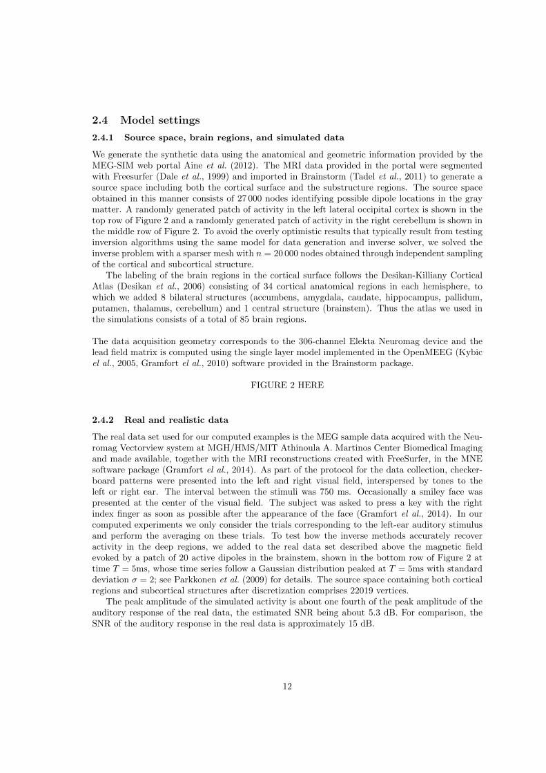
We generate the synthetic data using the anatomical and geometric information provided by theMEG-SIM web portal Aine et al. (2012). The MRI data provided in the portal were segmentedwith Freesurfer (Dale et al., 1999) and imported in Brainstorm (Tadel et al., 2011) to generate asource space including both the cortical surface and the substructure regions. The source spaceobtained in this manner consists of 27 000 nodes identifying possible dipole locations in the graymatter. A randomly generated patch of activity in the left lateral occipital cortex is shown in thetop row of Figure 2 and a randomly generated patch of activity in the right cerebellum is shown inthe middle row of Figure 2. To avoid the overly optimistic results that typically result from testinginversion algorithms using the same model for data generation and inverse solver, we solved theinverse problem with a sparser mesh with n = 20 000 nodes obtained through independent samplingof the cortical and subcortical structure.
The labeling of the brain regions in the cortical surface follows the Desikan-Killiany CorticalAtlas (Desikan et al., 2006) consisting of 34 cortical anatomical regions in each hemisphere, towhich we added 8 bilateral structures (accumbens, amygdala, caudate, hippocampus, pallidum,putamen, thalamus, cerebellum) and 1 central structure (brainstem). Thus the atlas we used inthe simulations consists of a total of 85 brain regions.
The data acquisition geometry corresponds to the 306-channel Elekta Neuromag device and thelead field matrix is computed using the single layer model implemented in the OpenMEEG (Kybicel al., 2005, Gramfort el al., 2010) software provided in the Brainstorm package.
FIGURE 2 HERE
2.4.2 Real and realistic data
The real data set used for our computed examples is the MEG sample data acquired with the Neu-romag Vectorview system at MGH/HMS/MIT Athinoula A. Martinos Center Biomedical Imagingand made available, together with the MRI reconstructions created with FreeSurfer, in the MNEsoftware package (Gramfort el al., 2014). As part of the protocol for the data collection, checker-board patterns were presented into the left and right visual field, interspersed by tones to theleft or right ear. The interval between the stimuli was 750 ms. Occasionally a smiley face waspresented at the center of the visual field. The subject was asked to press a key with the rightindex finger as soon as possible after the appearance of the face (Gramfort el al., 2014). In ourcomputed experiments we only consider the trials corresponding to the left-ear auditory stimulusand perform the averaging on these trials. To test how the inverse methods accurately recoveractivity in the deep regions, we added to the real data set described above the magnetic fieldevoked by a patch of 20 active dipoles in the brainstem, shown in the bottom row of Figure 2 attime T = 5ms, whose time series follow a Gaussian distribution peaked at T = 5ms with standarddeviation σ = 2; see Parkkonen et al. (2009) for details. The source space containing both corticalregions and subcortical structures after discretization comprises 22019 vertices.
The peak amplitude of the simulated activity is about one fourth of the peak amplitude of theauditory response of the real data, the estimated SNR being about 5.3 dB. For comparison, theSNR of the auditory response in the real data is approximately 15 dB.
12

2.5 Setting of IAS parameters
As shown in Sections 2.1-2.2, in the IAS algorithm the user has to assign the values of the threeparameters β, θmax, k and of δ in the local anatomical prior matrix Cj . The choice of all the fourparameters values can be driven by their physiological interpretation.
The hyperparameter β > 52 control the focality of the reconstructed sources: when β approaches
the limit value 52 , the reconstructed brain activity becomes more and more focal. Let us define
η = β − 52 . Several numerical simulations suggest that a reasonable values of η should range
between 0.1 and 0.001 (cf. Calvetti et al. (2015)), depending on whether we aspect less or morefocal sources: in the following tests, where we assume focal sources, we set η = 0.001.
The parameter θmax is used to avoid unrealistic high values of the dipole variances. Reliableestimates for the maximum dipole variance have been reported in the literature, see, e.g., (Mosherel al., 1993); alternatively, a heuristic criterion is to truncate the values of the variance retainingjust those values below the threshold θmax = 0.9 maxj(θj). The goodness of this choice has beenconfirmed with extensive simulations (cf. Calvetti et al. (2015)).
The parameter k is related to the number of sources we expect to be active. A direct compu-tation shows that ξ =
∑nj=1 pk/k assumes values between 0.5 and 0.2 when k varies from 1 to 10,
therefore a value of ξ in this interval is a good choice if we do not have any prior information onthe number of active sources. If we assume that only one source is active, we can set ξ = 1 (seethe Appendix). Although when testing with synthetic data we know exactly the number of activesources, we set ξ = 1 in all the tests we performed to show that this choice is a good initial guessfor both single and multiple source distributions.
The last parameter to be set in IAS is δ that accounts for possible inaccuracy in the segmentationof the cortical/subcortical surface normals. If the directions of the normals would be exact, δ couldbe set equal to zero; in the realistic case the anatomical data extracted from the MRI are not fullyaccurate so that the normal should be considered a preferred direction. To allow the dipoles tofollow quasi-normal orientation, we choose a small value of δ. Several numerical tests show that agood choice is δ = 0.05 (cf. (Calvetti et al., 2015)).
The tests in the following section show the effectiveness of our settings.
3 Results
3.1 Synthetic data tests
In this section, we systematically test the sensitivity and specificity, in the sense explained earlier,of the IAS MEG inverse solver algorithm using the validation tools described in the previoussection with synthetic data sets. For the sake of comparison, we run the same tests with otherthree standard MEG solvers, the weighted Minimum Norm Estimate (wMNE) (Lin el al., 2006a,Gramfort el al., 2014), the dynamic Statistical Parametric Mapping (dSPM) (Dale et al., 2000)and sLORETA (Pasqual-Marqui, 1999).
3.2 Performance via BR-ALI maps: synthetic data, single activity patch
The first suite of computed experiments is designed to assess whether and how the location of theBR where the activity occurs affects the quality of the IAS reconstruction. In order to provide ameasure that is robust over patches with different anatomical characteristics, for each one of the85 BRs specified by the selected atlas, we generate a sample of K = 100 patch activities by therandom process described in Section 2.3.1, calculate the magnetic field measured by the sensors,and add to the latter synthetic brain noise generated as described in Section 2.3.2. For each sampleproblem, we reconstruct the activity a with the IAS algorithm described in Section 2.1, as well as
13

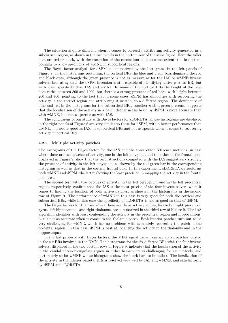
with the wMNE, DSPM and sLORETA algorithms as implemented in Brainstorm. For the lastthree algorithms we used default parameters, i.e. SNRdb = 3 and loose orientation. The resultsof the reconstructions are summarized in the average BR-ALI vectors and visualized in the formof histograms with whiskers indicating the marginal standard deviation around the mean. Anexample of activity reconstructions provided by the different methods for the patch activities inthe lateral occipital region and in the cerebellum shown in Figure 2 can be found in Figures 4 and6, respectively.
Figure 3 shows the average BR-ALI vectors when the active patch is in the left lateral occipitalcortex and the MEG inverse problem is solved with the IAS algorithm (top left), wMNE (topright), dSPM (bottom left) and sLORETA (bottom right), respectively. The results for the BRs inthe left hemisphere are shown in red, those for the BRs in the right hemisphere in black. Figure S1displays the histograms relative to the case where the active patch is in the frontal pole corticalregion in the right hemisphere.
FIGURE 3 HEREFIGURE 4 HEREFIGURE 5 HEREFIGURE 6 HERE
The deeper into the brain the active patch is, the more difficult we expect the mapping from theMEG data to the current dipoles to be. Figure 5 displays the histograms relative to 100 simulationswith the active patch located in the right portion of the cerebellum. Compared to the previoustests, the real challenge here arises from the distance of the activity region from the receivers.
The amygdala, a subcortical structure which is part of the limbic system, is believed to beinvolved in attentional and emotional processes and in the formation of memories. Its remotelocation and small dimensions add to the challenge of localizing activity confined into this regionfrom MEG data. Figure S2 displays the histograms for the four inverse methods relative to thecase where the active patch is confined to the left amygdala.
The four reported results are a representative subset of the performance of the four differentinverse solvers in cortical and subcortical brain regions.
3.3 Bayes factor analysis: synthetic data, single activity patch
To assess the IAS algorithm and to compare it to that of the other three MEG inverse solversconsidered in this study, we begin by performing a Bayes factor analysis with MEG data generatedaccording to the procedure described in Section 2.3.1 with a single activity patch. After generatingan ensemble of K = 20 randomly generated patches of activity restricted to a given BR, we computethe corresponding low noise synthetic data set, estimate the activity pattern with each inversionalgorithm and compute the corresponding Bayes factors, thus testing the evidence supporting thecorrect identification of the active area in the reconstruction. For each of the 20 active patchesin the sample, we draw 100 random spheres as competing alternative to the hypothesis that theactivity is in the BR where it actually occurs, for a total of 2 000 Bayes factors per BR.
The summary of the Bayes factor analysis for each active BR can be represented graphicallyin the form of a histogram with four bins, recording the number of occurrence of the four levelsof evidence (6) supporting the correct identification of the activity. The more occurrences thereare in the two top categories, the more reliable the algorithm is at correctly identifying the area ofactivity. For a easier visual assessment, we color coded the bars indicating the numbers of timesa Bayes factor falls into one of the four categories, using green for Bayes factors greater than 10(overwhelming support of the hypothesis that the active patch is indeed in that BR), blue forBayes factors between 3 and 10 (strong support), red for Bayes factors between 1 and 3 (weaksupport) and black for Bayes factor smaller than 1, in which case the support is for the hypothesisthat the active patch is not in that BR. A prevalence of green and blue indicates a strong support
14
of the hypothesis that the activity has been detected in the correct region, while a dominance ofblack and red suggests poor identification of active areas. Figure 7, 8 show the results for allcortical and subcortical BRs included in the atlas when performing the inverse mapping with thefour inverse solvers.
FIGURE 7 HEREFIGURE 8 HERE
3.4 Bayes factor analysis: Multiple activity patches
We extend the Bayes factor analysis to the case where several patches are active simultaneouslyin different BRs by performing a suite of four different tests. In the first two tests, we generatetwo randomly determined activity patches: In the first one, the activity patches are in the leftcerebellum and the left prefrontal cortex, and in the second one, in the left amygdala and the leftprefrontal cortex. In both cases one of the patches is cortical and the other one deep in the brain.In the third set of tests, the simulated data arises from three activated patches, located in theleft precuneous, right precuneous and left inferior parietal cortex. In the last protocol we generateactivity patches in the six different regions comprising the default mode network (DMN), namelyin the left precuneus, right precuneus, left inferior parietal cortex, right inferior parietal cortex,left caudal anterior cingulate and right caudal anterior cingulate regions.
As in the case of a single active BR, we generate K = 20 independent activity patterns in theselected BRs, compute the corresponding low noise data, solve the inverse problem with the fourdifferent algorithms and test the support of the hypothesis H0 for each of the activated regionsindividually with M = 100 independently drawn competing spheres Bm. Observe that when wetest the hypothesis H0 for a single selected brain region while the data are generated by severalactive sources, the magnetic field due to the additional sources represent high amplitude brainnoise masking the signal from the source of interest.
The top row of Figure 9 shows the histograms of the Bayes factors, binned and color codedaccording to the strength of evidence (6), corresponding to the four different inverse solvers in thecase when the active patches are in the left amygdala and in the left frontal pole. The second rowof Figure 9 shows the histograms of the Bayes factors for the four different inverse solvers in thecase when the active patches are in the left cerebellum and in the left precentral cortex.
The histograms of the Bayes factors for the four inverse solvers when there are three activepatches located in the left hippocampus, precentral gyrus and right thalamus are displayed in thethird row of Figure 9. Finally, the histograms for the Bayes factors corresponding to the differentsolvers in the case where there are active patches in the six different BRs in the DMN are displayedin the two bottom rows of Figure 9.
FIGURE 9 HERE
3.5 Reconstruction of the brain activity from real data
Finally, we apply the different inverse solvers to the real data, augmented with realistic activityin the brainstem as explained in Section 2.4.2. Figures 10 and 11 show respectively the averageBR-ALI vectors at times T = 5 ms and T = 100 ms for the four inverse solvers. In Figures 12 and15 we show ten axial slices of the two reconstructions of the brain activity at times T = 5 ms andT = 100 ms obtained using the IAS (left) and the wMNE (right) inverse solvers. In Figure 13 and16 we show the corresponding reconstructions obtained by dSPM (left) and sLORETA (right). InFigures 14, 17 we show the 3D reconstructions obtained at T = 5 ms and T = 100 ms by the fourinverse solvers.
FIGURE 10 HEREFIGURE 11 HERE
15
FIGURE 12 HEREFIGURE 13 HEREFIGURE 14 HEREFIGURE 16 HEREFIGURE 16 HEREFIGURE 17 HERE
4 Discussion
4.1 BR-ALI maps
The sparsity of the BR-ALI map is a good indicator for the sensitivity and specificity of an inversesolver: The more concentrated the histograms are on the active areas, the more likely it is thatthe activity is correctly identified without too much of confounding. In general, we expect a highersensitivity and specificity for BRs closer to the sensors than in BRs deep in the brain, as confirmedby the computed experiments.
4.1.1 Single patch in cortical BRs
It emerges clearly from the panels in the top row of Figure 3 that the IAS and wMNE inversesolvers have high sensitivity to activation restricted to the left lateral occipital cortex, indicatedby the outstanding histogram bar, and that the confounding is confined mostly to anatomicallyproximal regions, most notably the nearby pericalcarine fissure in the same hemisphere. Neitheralgorithm suggest any significant activity in the right hemisphere, or in the deep brain structures.In the BR-ALI vector computed by the dSPM or sLORETA algorithms, on the other hand, theleft lateral occipital BR is not as clearly identifiable, and the likely locus of activity is attributedto several nearby BRs in the same hemisphere, e.g., the nearby pericalcarine fissure, lingual, andcuneous BRs. Some of the brain activity is suggested also in the right hemisphere and in the deepbrain structures. Overall, the performance of the IAS algorithm appears to be significantly moresimilar to that of wMNE than to dSPM or sLORETA, the latter ones producing more confoundingactivity.
The suite of simulations with the activity confined to the right frontal pole region confirmsthe conclusions of the relative sensitivity of the four different approaches. The correspondingBR-ALI vectors, visualized in the form of histograms in Figure S1, show that both the IAS andwMNE algorithms reconstruct a substantial portion of the dipole activity in the right frontal pole,while finding some activity also in the nearby left frontal pole and, to a lesser extend, to themedial orbitofrontal cortex, also anatomically close. In neither case, any significant leakage ofthe reconstructed activity to BRs in the deep brain occurs. The localization of the active BR ismuch weaker for the dSPM and sLORETA methods, whose BR-ALI vectors indicate a smearingof the reconstructed activity over several BRs, including subcortical ones. In this test sLORETAappeared to recognize the BR where the signal generating the data came from better than dSPMwhich attributes the highest average activity to the rostral anterior cingulate cortex.
The first two tests are representative for the four methods when the data correspond to activityin a restricted patch located in a cortical BR, with IAS and wMNE performing quite satisfactorilywhen it comes to identifying the active BR, while dSPM and sLORETA have the tendency to favoractivity in deeper regions of the brain.
16

4.1.2 Single patch in subcortical BRs
The sensitivities of the four solvers when the active patch is confined to the right cerebellum aresummarized in Figure 5. As in the case of active patches in cortical regions, the attribution of thebrain activity to the correct BR is less confounded when the inverse problem is solved using theIAS or wMNE algorithms. The BR-ALI vectors corresponding to these two algorithms point moreclearly to the right cerebellum, with a little activity smeared to the left cerebellum and brainstem.The BR-ALI vectors for the dSPM and sLORETA inversion methods, on the other hand, tendto distribute the activity in the deeper regions of the brain, without the cerebellum standing outclearly among them. Moreover, a substantial fraction of the activity is mapped to cortical regions,e.g., lingual, parahippocampal and pericalcarine gyrus, suggesting potential problems when itcomes to specificity.
The same patterns are observed when the active patch is in the left amygdala. As shown inFigure S2, the IAS inverse solver is quite effective at identifying the presence of activity in the leftamygdala, with some leakage to the anatomically adjacent left temporal pole and left entorhynalcortex. The wMNE BR-ALI histogram does not show a localization to the left amygdala of theactivity; instead, the activity is distributed over the left hemisphere, with a slight preference forthe BRs closer to the left amygdala. The BR-ALI vectors relative to dSPM and sLORETA, on theother hand, map the reconstructed activity without much distinction onto all BRs correspondingto internal structures, and a few cortical BRs in the proximity of the left amygdala, suggesting abias towards regions of the brain away from the surface.
4.2 Bayes factor analysis
The Bayes factor analysis is based on the counts of how often, and at which level, out of the 2 000tests per brain region, the reconstruction of the brain activity by a given algorithm supports thehypothesis that the activity is indeed in the correct region. Due to our choice of color coding, wecan be confident that the activity within a BR when the corresponding histogram has taller greenor blue bars can be identified by the inverse solver rather unequivocally, while taller black or redbars are an indication that activity in that BR is likely to be erroneously attributed to activity inanother part of the brain.
4.2.1 Single active patch
The overwhelming predominance of green in the left panels of Figure 7, displaying the histogramsof the Bayes factors for the cortical BRs, is a strong indicator that the solution of the MEG inverseproblem produced by the IAS algorithm is much more likely to find active current dipoles in thecorrect BR than in other regions. A slightly lesser dominance of the green and blue bars for theinsula and isthmus cingulate BR suggests that activity concentrated in either of these two regionsmay have a slightly larger tendency to be incorrectly attributed elsewhere. In most of the Bayesfactors histograms for the subcortical BRs the green and blue bars dominate over the red and blackones, with the exception of the thalamus and, to a lesser extent, the caudate gyrus, where the redand black take over, suggesting that the IAS has difficulties to identify unequivocally activitylocalized in this BR.
In the histograms of the classification of the Bayes factors for the wMNE algorithm, shown inthe right panels of Figure 7, the green and blue bars tend to be more prominent than the red andblack ones in the top row, although not as markedly as for IAS. This is an indication that whenthe measured signal comes from a patch in a cortical BR, the solution computed by wMNE islikely to be concentrated in the correct cortical region, with the exceptions for the caudal anteriorcingulate, insula, isthmus cingulate, parahippocampal, posterior cingulate and rostral anteriorcingulate regions.
17
The situation is quite different when it comes to correctly attributing activity generated in asubcortical region, as shown in the two panels in the bottom row of the same figure. Here the tallerbars are red or black, with the exception of the cerebellum and, to some extent, the brainstem,pointing to a low specificity of wMNE in subcortical regions.
The Bayes factor analysis for dSPM is summarized by the histograms in the left panels ofFigure 8. In the histograms pertaining the cortical BRs the blue and green bars dominate the redand black ones, although the green presence is not as massive as for the IAS or wMNE inversesolvers, indicating that the dSPM inversion is still capable of identifying active cortical BR, butwith lower specificity than IAS and wMNE. In many of the cortical BRs the height of the bluebars varies between 800 and 1000, but there is a strong presence of red bars, with height between200 and 700, pointing to the fact that in some cases, dSPM has difficulties with recovering theactivity in the correct region and attributing it instead, to a different region. The dominance ofblue and red in the histograms for the subcortical BRs, together with a green presence, suggeststhat the localization of the activity in a patch deeper in the brain by dSPM is more accurate thanwith wMNE, but not as precise as with IAS.
The conclusions of our study with Bayes factors for sLORETA, whose histograms are displayedin the right panels of Figure 8 are very similar to those for dSPM, with a better performance thanwMNE, but not as good as IAS, in subcortical BRs and not as specific when it comes to recoveringactivity in cortical BRs.
4.2.2 Multiple activity patches
The histograms of the Bayes factor for the IAS and the three other reference methods, in casewhere there are two patches of activity, one in the left amygdala and the other in the frontal pole,displayed in Figure 9, show that the reconstructions computed with the IAS suggest very stronglythe presence of activity in the left amygdala, as shown by the tall green bar in the correspondinghistogram as well as that in the cortical frontal pole. In this experiment, sLORETA outperformsboth wMNE and dSPM, the latter showing the least precision in mapping the activity in the frontalpole area.
The second test with two patches of activity, in the left cerebellum and in the left precentralregion, respectively, confirm that the IAS is the most precise of the four inverse solvers when itcomes to finding the location of both active patches, as shown in the histograms in the secondrow of Figure 9. The performance of wMNE in this case is very good for both the cortical andsubcortical BRs, while in this case the specificity of sLORETA is not as good as that of dSPM.
The Bayes factors for the case where there are three active patches, located in right precentralgyrus, left hippocampus and right thalamus, are summarized in the third row of Figure 9. The IASalgorithm identifies with least confounding the activity in the precentral region and hippocampus,but is not as accurate when it comes to the thalamic patch. Both interior patches turn out to bevery challenging for wMNE, which has no problems with accurately recovering the patch in theprecental region. In this case, dSPM is best at localizing the activity in the thalamus and in thehippocampus.
In the last protocol with Bayes factors, the MEG signal came from six active patches locatedin the six BRs involved in the DMN. The histograms for the six different BRs with the four inversesolvers, displayed in the two bottom rows of Figure 9, indicate that the localization of the activityin the caudal anterior cingulate region in either hemisphere is challenging for all methods, andparticularly so for wMNE whose histograms show the black bars to be tallest. The localization ofthe activity in the inferior parietal BRs is resolved very well by IAS and wMNE, and satisfactorilyby dSPM and sLORETA.
18

4.3 Real data: IAS favors sparse solution
Figures 10 and 11 show the BR-ALI vectors for the four inverse methods at times T=5 ms andT=100 ms, respectively. At T=5 ms all inverse methods find activity also but not only in thebrainstem region: the estimated activities using sLORETA and dSPM are mutually very similar,suggesting activation also in the amygdala and in the parahippocampal cortex; the deep activityis dominating over cortical activity in the reconstructions. The reconstructed activity by wMNE,compared to IAS, is more smooth, while IAS finds activity also in cerebellum. At T=100 ms, IASsuggests activity in the temporal region, mainly in the upper bank of the superior temporal cortexand in the transverse temporal region, that are part of the primary auditory cortex. The IAS MEGsolution shows activity in the superior temporal regions of both hemispheres, while when usingother methods such bilaterality is not evident. In general, the dSPM and sLORETA algorithmsseem to be in favor of activity deeper in brain, and the spatial smoothing characteristics of thealgorithms is clearly visible.
4.4 Methodological issues and future work
As shown in Section 2.5, the choice of the parameters in the IAS algorithm can be driven by theirphysiological meaning. Several tests we performed show that the reconstructed activity map is notvery sensitive to the values of the parameters δ, θmax and ξ. The values we used in the tests arereasonable for most applications in neuroscience. Thus, the parameter that the user has really toselect is η = β − 5
2 . Since η controls the sparsity of the reconstruction, its choice is related to thea priori knowledge we have on the protocol of the neuroscience experiment under study. Valuesof η in the order of 0.1 favor more spread reconstruction and for these values the IAS algorithmproduces activity maps very similar to the maps obtained by the wMNE algorithm. On the otherhand, values in the order of 0.001 favor focal reconstructions, which is the more interesting case inneuroscience studies, especially when deep brain sources are involved.
Further studies of the performance of the IAS algorithm on the localization of deep brainactivity will be done in the future, including the use of a more accurate model for describing deepbrain sources, e.g., the model proposed in Attal et al. (2012), Attal and Schwartz (2013) or themixed source space model available in the MNE software1. In this case, different values of theparameter η for cortical and subcortical regions can be used in order to increase the sensitivityof the algorithm to deep sources. Finally, to take into account the imprecision due the use of anaveraged physiological atlas that cannot reproduce exactly the individual anatomy, one can usesome mathematical methods related to fuzzy logic (see, e.g., (Algorri and Flores-Mangas, 2004,Ciofolo and Barillot, 2009)).
The IAS algorithm described in this paper is designed for a single-time slice analysis: thealgorithm is re-initialized each time and does not retain any previous information. Actually, one ofthe main advantage of the MEG devices is in that they can measure the neuromagnetic field witha high temporal resolution. In order to deal with MEG time series some preliminary results showthat when the IAS algorithm starts from a θ∗ that is related to the values of θj at the previoustime step, the rate of convergence of the algorithm is increased. Then, for a further analysis wecan model θ as a Markov process, so the estimation of θ at time t depends just on the value of θat time t− δt.
1http://martinos.org/mne
19

5 Conclusions
Finding a robust metric for assessing the performance of an inverse solver in MEG is not a simpletask. Algorithms that are based on the goal of localizing single dipoles may be judged accordingto the precision of the localization, but such metric may not be a judicious one for methods thatestimate distributed sources. Vice versa, single dipole methods may have a limited success whendistributed activities are to be estimated. In this paper we propose a metric for the algorithmassessment based on the reliability of an algorithm to identify active brain regions, superficial anddeep, regardless of whether a single or several active regions occur. As pointed out, the BR-ALIanalysis has a formal similarity with the resolution matrix analysis which is widely used as a basis ofperformance analysis, and allows the computation of simple measures for performance: Resolutionindex (RI), dipole resolution error (DLE), and spatial dispersion (SD), see Molins et al. (2008) andAttal and Schwartz (2013), Hedrich et al. (2017). The precision of finding a single dipole is not ofconcern here, although the focality of the reconstructions helps discerning between brain regionsthat are anatomically close. One of the messages of the analysis is that an algorithm such as IASfavoring focal solutions produces less confounding reconstructed activity in the anatomically closeregions, reducing the ambiguity in the interpretation of the reconstruction. To avoid the pitfallof anecdotal successes, the methodology is based on extensive independent Monte Carlo sampling,and the results are processed into a form of first and second order statistics, and Bayes factoranalysis. The long-term goal of this work is to build reliable uncertainty quantification tools toanalyze extensive data sets with non-event based brain data, e.g., various resting states or statesof consciousness, brain connectivity, or fingerprinting of diseased or abnormal states. Assessmentof success rates of algorithms as presented here, as opposed to precision case studies with activitylocalization, is in line with the current algorithm testing paradigm in data mining and big dataanalysis. The proposed methodology was tested with four inverse solvers, one of which is therecently developed IAS algorithm, and three standard methods. Our conclusion is that the IASmethod seems to perform relatively consistently in the tasks that it is originally designed for, thatis to identify both active cortical and deep brain regions without a significant confounding beyondthe inevitable leakage of the estimated activity to anatomically close regions, which is due to theinherent ill-posedness of the problem. The comparison of the algorithm was done against threestandard MEG algorithms without detailed tuning of the default settings. A more comprehensivemeta-analysis should include the optimization of the model parameters as well as the inclusion ofother algorithms favoring focal solutions, but is beyond the scope of this work.
Appendix: Interpretation of hyperparameters
In Calvetti et al. (2015), the interpretation of the hyperparameters β ∈ R and θ∗ ∈ RN wasdiscussed: It was shown that β allows the user to control the sparsity of the IAS solution, while theempirical Bayesian approach provided a way to relate θ∗ to the sensitivity scaling. We summarizehere the analysis on hyperparameters, developing the discussion of θ∗ further, so that the parametertuning can be done easily and semi-automatically.
Parameter β and control of sparsity
In Calvetti et al. (2015), it was proved (Theorem 2.1) that the sequential minimization that consti-tutes the core of the IAS algorithm can be interpreted as a fixed point iteration to find a minimizerQ = [~q1, ~q2, . . . , ~qn]T ∈ R3n of the energy functional (3),
Q = argmin{E(Q,S(Q))
}, Θ = S(Q),
20

where Θ = [θ1; θ2; . . . , θn] ∈ Rn, and S : R3n → Rn is defined componentwise as
θj = Sj(~qj) = θ∗j
ηj
2+
√η2j4
+‖~qj‖2Cj
2θ∗j
, ηj = βj −
5
2, 1 ≤ j ≤ n.
Furthermore, it was shown that if we write βj = 5/2 + η, 1 ≤ j ≤ n, then, as η → 0+, we have theasymptotic expression
E(Q,S(Q)) =1
2‖b−
n∑
j=1
Mj~qj‖2Σ +√
2
n∑
j=1
‖~qj‖Cj√θ∗j
+O(η). (7)
In particular, the penalty term in the above expression is a weighted `1-norm for the dipole ampli-tudes that are measured in the metric defined by the anatomical prior matrices Cj . This argumentdemonstrates that at the limit, the IAS algorithm provides an effective algorithm for finding aweighted Minimum Current Estimate (MCE), with the modification given by the anatomical prior(Uutela et al., 1999). In conclusion, we see that the role of the hyperparameter β is to control thesparsity of the IAS estimate. In Calvetti et al. (2015), this effect was demonstrated using numericalsimulations.
Parameter θ∗ and sensitivity
The asymptotic expression (7) is indicative also from the point of view of the interpretation of θ∗j .It is well-known that MEG algorithms based on penalized minimization of the fidelity to data tendto favor superficial sources, and to compensate this effect, a sensitivity weight is often introduced,see, e.g. Lin el al. (2006a). From the Bayesian point of view, sensitivity weighting is a problematicpractice, since traditionally the prior should be independent of the observation model, a conditionthat the sensitivity weight does not satisfy. However, it is possible to find a satisfactory Bayesianinterpretation for θ∗j so that it effectively works as a sensitivity weight. The connection betweensensitivity and hypermodels is built through the analysis of the signal-to-noise ratio as follows.Consider the linear forward model
b = MQ+ ε =
n∑
j=1
Mj~qj + ε = b0 + ε, ε ∼ N (0,Σ).
To estimate the expected power of the noiseless signal appearing in the signal-to-noise ratio definedin (4), observe that from the prior model, conditional on Θ ∈ Rn, we have
E{‖b0‖2 | Θ} =
n∑
j=1
θjtrace(MjCjM
Tj
)=
n∑
j=1
θj‖MjC1/2j ‖2F,
where the subscript refers to the Frobenius norm of the matrix. Furthermore, by using the gammahyperprior model θj ∼ Γ(β, θ∗j ) for the vector Θ, we arrive at
E{‖b0‖2} =
n∑
j=1
E{θj}‖MjC1/2j ‖2F =
n∑
j=1
βθ∗j ‖MjC1/2j ‖2F.
The choice of the hyperparameters θ∗j must therefore be compatible of what we a priori assumeabout the distribution of the activity and the resulting SNR. To begin with, assume that we have
21

a reason to believe that only one source is active, but we do not know which one. Then, by thedefinition (4) of SNR, the active source j1 must satisfy
βθ∗j1‖Mj1C1/2j1‖2F = (SNR− 1)× trace(Σ), or θ∗j1 =
(SNR− 1)× trace(Σ)
β‖Mj1C1/2j1‖2F
.
This must be true, whichever the active source is, and if each source has equal probability to beactive, the exchangeability argument yields the scaling law
θ∗j =(SNR− 1)× trace(Σ)
β‖MjC1/2j ‖2F
, 1 ≤ j ≤ n.
This argument can be generalized to several, and unknown, number of active sources. Assumethat we believe that k of the sources are non-zero, but we do not know which ones. Denoting theindices to the active sources by j1, j2, . . . , jk, we must have
k∑
`=1
βθ∗j`‖Mj`C1/2j`‖2F = (SNR− 1)× trace(Σ). (8)
For the exchangeability argument, let us denote by γ ∈ Rn the vector with entries γj = βθ∗j ‖MjC1/2j ‖2F,
and by Pk ∈ Rnk×n the matrix such that the pth row contains exactly k entries equal to one, otherentries being zero, and each permutation appears only once in the matrix. Therefore, the numberof rows in Pk is nk = n!/(k!(n− k)!). Since we assume that (8) holds regardless of the selection ofthe active sources, the vector γ must satisfy the linear system
Pkγ = (SNR− 1)× trace(Σ)1nk,
where 1nk∈ Rnk denotes a vector with unit entries. The only possible solution of this system is
γj =(SNR− 1)× trace(Σ)
k,
and therefore, we arrive at the scaling law
θ∗j =1
k
(SNR− 1)× trace(Σ)
β‖MjC1/2j ‖2F
, 1 ≤ j ≤ n.
Finally, assume that we only have a prior idea of how many non-zero sources may be active,and we express this belief in a form of a probability density
P{# of active sources = k} = pk, 1 ≤ k ≤ n,where
∑k pk = 1. If we expect that out of the n dipoles, it is reasonable to expect that k = sn
are active, a binomial distribution can be used for pk, kk ∼ Binom(n, s), 0 < s < 1; in practice thebinomial can be approximated by a Poisson distribution, pk ∼ Poisson(k) with mean k providedby the user. Using the previous result, conditioned on k, we arrive at the scaling law
θ∗j =C
‖MjC1/2j ‖2F
, 1 ≤ j ≤ n,
with
C = (SNR− 1)× trace(Σ)
n∑
k=1
pkk.
This argument confirms that, in order to match the model with the SNR, the parameters θ∗j shouldindeed be chosen to be inversely proportional to the sensitivity.
22

Appendix: Construction of the activity patch
To select the vertices in the activity patch P, we first pick randomly a seed vertex from the BR ofinterest, then grow the patch by adding iteratively the neighboring vertices, pruning off at each stepthose that fall outsize the pertinent BR, and stopping the process as soon as the desired numberNP of vertices have been included. The selected nodes along with the edges of the triangular meshform a local graph. To generate the activity in the patch, we start by computing a positive graphLaplacian of the patch, which is the matrix L ∈ RNP×NP with entries
Li,j =
−deg(vi) if i = j,1 if i 6= j and vi is adjacent to vj ,0 otherwise,
where deg(vi) is the number of the edges that terminate at the vertex vi.After defining a correlation length λ, given in units of the number of steps, we draw a random
amplitude vector by settingQ = (L + λ2INP )−1W,
where INP ∈ RNP×NP is the unit matrix and W ∈ RNP is a standard normal Gaussian randomvector, that is, W ∼ N (0, INP ). The amplitudes are scaled so that the amplitude of the dipole atthe seed vertex is one. Finally, we draw the dipole moment directions from the anatomical prior,making sure that adjacent dipoles are not pointing in the opposite sides of the cortex patch.
23

Acknowledgements
This work was completed during the visit of DC and ES at University of Rome “La Sapienza”(Visiting Researcher/Professor Grant 2015). The hospitality of the host university is kindly ac-knowledged. The work of ES was partly supported by NSF, Grant DMS-1312424. The work ofDC was partially supported by grants from the Simons Foundation (#305322 and # 246665) andby NSF, Grant DMS-1522334.
References
Aine CJ, Sanfratello L, Ranken D, Best E, MacArthur JA, Wallace T, Gilliam K, Donahue CH,Montano, R, Bryant, JE and others (2012) MEG-SIM: a web portal for testing MEG analysismethods using realistic simulated and empirical data. Neuroinformatics 10(2): 141–158
Algorri ME and Flores-Mangas F (2004) Classification of anatomical structures in MR brain imagesusing fuzzy parameters. IEEE Trans Biomed Engineering 51: 1599–1608
Auranen T, Nummenmaa A, Hamalainen MS, Jaaskelainen IP, Lampinen J,Vehtari A, Sams M(2005) Bayesian analysis of the neuromagnetic inverse problem with `p-norm priors. NeuroImage26: 870–884
Attal, Y, Maess B, Friederici A and David, O (2012) Head models and dynamic causal modeling ofsubcortical activity using magnetoencephalographic/electroencephalographic data. Rev Neurosci23: 141–158
Attal Y, Schwartz D (2013) Assessment of subcortical source localization using deep brain activityimaging model with minimum norm operators: a MEG study. PLoS One 8: e59856
Baillet S, Garnero L (1997) A Bayesian approach to introducing anatomo-functional priors in theEEG/MEG inverse problem. IEEE Trans BME 44:374–385
Baillet S, Mosher JC, Leahy RM (2001) Electromagnetic brain mapping. IEEE Signal Proc Mag18:14–30
Bernardo JM, Smith AFM (2004) Bayesian theory. John Wiley & Sons
Brette R and Destexhe A (2012) Handbook of neural activity measurement. Cambridge UniversityPress
Calvetti D, Pascarella A, Pitolli F, Somersalo E, Vantaggi B (2015) A hierarchical Krylov–Bayesiterative inverse solver for MEG with physiological preconditioning. Inverse Problems 31:125005
Calvetti D, Pitolli F, Somersalo E, Vantaggi B (2018) Bayes meets Krylov: preconditioning CGLSfor underdetermined systems. SIAM Rev 60: DOI 10.1137/15M1055061
Calvetti D, Hakula H, Pursiainen S, Somersalo E (2009) Conditionally Gaussian hypermodels forcerebral source localization. SIAM J Imag Sci 2: 879–909
Ciofolo, C and Barillot C (2009) Atlas-based segmentation of 3D cerebral structures with compet-itive level sets and fuzzy control. Medical Image Analysis 13: 456–470
Collins, D Louis and Zijdenbos, Alex P and Kollokian, Vasken and Sled, John G and Kabani, NoorJ and Holmes, Colin J and Evans, Alan C (1998) Design and construction of a realistic digitalbrain phantom. IEEE Trans BME 17: 463–468
24

Dale AM, Fischl B and Sereno MI (1999) Cortical surface-based analysis: I. Segmentation andsurface reconstruction. NeuroImage 9: 179–194
Dale MA, Liu AK, Fischl BR, Buckner RL, Belliveau JW, Lewine JD and Halgren E (2000)Dynamic statistical parametric mapping: combining fMRI and MEG for high-resolution imagingof cortical activity. Neuron 26: 55–67
de Munck JC, Vijn PCM and da Silva FH Lopes (1992) A random dipole model for spontaneousbrain activity. IEEE Trans BME 39: 791–804
Desikan RS , Segonne F, Fischl B, Quinn BT, Dickerson BC, Blacker D, Buckner RL, Dale, AM,Maguire RP, Hyman BT and others (2006) An automated labeling system for subdividing thehuman cerebral cortex on MRI scans into gyral based regions of interest. NeuroImage 31: 968–980
Gorodnitsky IF and Rao BD (1997) Sparse signal reconstruction from limited data using FOCUSS:A re-weighted minimum norm algorithm. IEEE Trans. on Signal Processing 45: 600–616
Gramfort A, Papadopoulos T, Olivi E and Clerc M (2010) Open MEEG: open source software forquasistatic bioelectromagnetics. Biomedical Engineering Online 9
Gramfort A, Luessi, M, Larson E, Engemann, DA, Strohmeier D, Brodbeck C, Parkkonen L andHamalainen MS (2014) NeuroImage 31: 446–460
Hedrich T, Pellegrino G, Kobayashi E, Lina JM and Grova G (2017) Comparison of the spatialresolution of source imaging techniques in high-density EEG and MEG. NeuroImage 175:531–544.
Henson RN, Mattout J, Phillips C and Friston KJ (2009) Selecting forward models for MEGsource-reconstruction using model-evidence. NeuroImage 46: 168–176
Henson, RN, Flandin G, Friston KJ and Mattout J (2010) A parametric empirical Bayesian frame-work for fMRI-constrained MEG/EEG source reconstruction. Human Brain Mapping 31: 1512–1531
Hamalainen MS, Hari R, Ilmoniemi RJ, Knuutila, J and Lounasmaa, OV (1993)Magnetoencephalography–theory, instrumentation, and applications to noninvasive studies ofthe working human brain. Rev Mod Phys. 65: 413–498
Hamalainen MS and Ilmoniemi RJ (1984) Interpreting measured magnetic fields of the brain:estimates of current distributions. Report TKK-F-A559
Huizenga HM, De Munck JaC, Waldorp LJ and Grasman RPPP (2002) Spatiotemporal EEG/MEGsource analysis based on a parametric noise covariance model. IEEE Trans BME 49: 533–539
Kass RE and Raftery AE (1995) Bayes factors. JASA 90: 773–795
Variational Bayesian inversion of the equivalent current dipole model in EEG/MEG. Kiebel SJ,Daunizeau J, Phillips, C and Friston KJ (2008) NeuroImage 39: 728–741
Kybic, J, Clerc M, Abboud T, Faugeras O, Keriven R and Papadopoulos T (2005) A commonformalism for the integral formulations of the forward EEG problem. IEEE Trans Med Imaging24: 12–28
25

Lin FH, Witzel T, Ahlfors SP, Stufflebeam SM, Belliveau JW and Hamalainen, MS (2006) Assessingand improving the spatial accuracy in MEG source localization by depth-weighted minimum-norm estimates. NeuroImage 31: 160–171
Lin FH, Belliveau JW, Dale AM and Hamalainen MS (2006) Distributed current estimates usingcortical orientation constraints. Human Brain Mapping 27: 1–13
Lopez,JD, Litvak V, Espinosa JJ, Friston K, Barnes GR (2014) Algorithmic procedures forBayesian MEG/EEG source reconstruction in SPM. NeuroImage 84: 476–487
Lucka F, Pursiainen S, Burger M and Wolters CH (2012) Hierarchical Bayesian inference for theEEG inverse problem using realistic FE head models: depth localization and source separationfor focal primary currents. NeuroImage 61: 1364–1382
Mattout J, Phillips C, Penny WD, Rugg MD, Friston KJ (2006) MEG source localization undermultiple constraints: an extended Bayesian framework. NeuroImage 30: 753–767
Molins A, Stufflebeam SM, Brown EN and Hamalainen MS (2008) Quantification of the benefitfrom integrating MEG and EEG data in minimum ?2-norm estimation. Neuroimage, 42(3):1069-1077.
Mosher JC, Spencer ME, Leahy RM and Lewis PS (1993) Error bounds for EEG and MEG dipolesource localization. Electroenceph clin Neurophysiol 86: 303–321
Nagarajan SS, Portniaguine O, Hwang D, Johnson C, Sekihara K (2006) Controlled support MEGimaging. NeuroImage 33: 878–885
Nummenmaa A, Auranen T, Hamalainen MS, Jaaskelainen IP, Lampinen J, Sams M, VehtariA (2007) Hierarchical Bayesian estimates of distributed MEG sources: theoretical aspects andcomparison of variational and MCMC methods. NeuroImage 35: 669–685
Nummenmaa A, Auranen T, Hamalainen MS, Jaaskelainen IP, Lampinen J, Sams M, VehtariA (2007) Automatic relevance determination based hierarchical Bayesian MEG inversion inpractice. NeuroImage 3: 876–889
Owen JP, Wipf DP, Attias HT, Sekihara K, Nagarajan SS (2012) Performance evaluation of theChampagne source reconstruction algorithm on simulated and real M/EEG data. NeuroImage60: 305–323
Parkkonen L, Fujiki N, Makela JP (2009) Sources of auditory brainstem responses revisited: con-tribution by magnetoencephalography. Human Brain Mapping 30:1772–1782.
Pascual-Marqui RD (1999) Review of methods for solving the EEG inverse problem. Int J Bioelec-tromagn 1:75–86
Sato M, Yoshioka T, Kajihara S, Toyama K, Goda N, Doya K, Kawato M (2004) HierarchicalBayesian estimation for MEG inverse problem. NeuroImage 23:806–826
Bayesian model selection for group studies. Stephan KE, Penny WD, Daunizeau J, Moran RJ andFriston KJ (2009) NeuroImage 46: 1004–1017
Tadel F, Baillet S, Mosher JC, Pantazis D, Leahy RM (2011) Brainstorm: a user-friendly applica-tion for MEG/EEG analysis. Comp Intell Neurosci 2011:879716.
Trujillo-Barreto NJ, Aubert-Vazquez E, Valdes-Sosa PA (2004) Bayesian model averaging inEEG/MEG imaging. NeuroImage 21:1300–1319
26

Uutela K, Hamalainen MS, Somersalo E (1999) Visualization of magnetoencephalographic datausing minimum current estimates. NeuroImage 10:173–180
Wagner M, Fuchs M, Kastner J (2004) Evaluation of sLORETA in the presence of noise andmultiple sources. Brain Topography 16:277–280
Wipf D, Nagarajan S (2009) A unified Bayesian framework for MEG/EEG source imaging. Neu-roImage 44:947–966
Wipf DP, Owen JP, Attias HT, Sekihara K, Nagarajan SS (2010) Robust Bayesian estimationof the location, orientation, and time course of multiple correlated neural sources using MEG.NeuroImage 49:641–655
Vorwerk J, Cho JH, Rampp S, Hamer H, Knosche TR and Wolters CH (2014) A guideline for headvolume conductor modeling in EEG and MEG. NeuroImage 100: 590–607
27

D. Calvetti REFERENCES
Figure 2
43
Figure 2: Top row: A randomly generated patch of activity in the left lateral occipital cortex regionof the brain. Middle row: A randomly generated patch of activity in right cerebellum. Bottomrow: A randomly generated patch of activity in the brainstem.
28

D. Calvetti REFERENCES
25 20 15 10 5 0 0 5 10 15 20 25
BANKSSTS
CAUDALANTERIORCINGULATE
CAUDALMIDDLEFRONTAL
CUNEUS
ENTORHINAL
FRONTALPOLE
FUSIFORM
INFERIORPARIETAL
INFERIORTEMPORAL
INSULA
ISTHMUSCINGULATE
LATERALOCCIPITAL
LATERALORBITOFRONTAL
LINGUAL
MEDIALORBITOFRONTAL
MIDDLETEMPORAL
PARACENTRAL
PARAHIPPOCAMPAL
PARSOPERCULARIS
PARSORBITALIS
PARSTRIANGULARIS
PERICALCARINE
POSTCENTRAL
POSTERIORCINGULATE
PRECENTRAL
PRECUNEUS
ROSTRALANTERIORCINGULATE
ROSTRALMIDDLEFRONTAL
SUPERIORFRONTAL
SUPERIORPARIETAL
SUPERIORTEMPORAL
SUPRAMARGINAL
TEMPORALPOLE
TRANSVERSETEMPORAL
ACCUMBENS
AMYGDALA
CAUDATE
CEREBELLUM
HIPPOCAMPUS
PALLIDUM
PUTAMEN
THALAMUS
BRAINSTEM
(a) IAS25 20 15 10 5 0 0 5 10 15 20 25
BANKSSTS
CAUDALANTERIORCINGULATE
CAUDALMIDDLEFRONTAL
CUNEUS
ENTORHINAL
FRONTALPOLE
FUSIFORM
INFERIORPARIETAL
INFERIORTEMPORAL
INSULA
ISTHMUSCINGULATE
LATERALOCCIPITAL
LATERALORBITOFRONTAL
LINGUAL
MEDIALORBITOFRONTAL
MIDDLETEMPORAL
PARACENTRAL
PARAHIPPOCAMPAL
PARSOPERCULARIS
PARSORBITALIS
PARSTRIANGULARIS
PERICALCARINE
POSTCENTRAL
POSTERIORCINGULATE
PRECENTRAL
PRECUNEUS
ROSTRALANTERIORCINGULATE
ROSTRALMIDDLEFRONTAL
SUPERIORFRONTAL
SUPERIORPARIETAL
SUPERIORTEMPORAL
SUPRAMARGINAL
TEMPORALPOLE
TRANSVERSETEMPORAL
ACCUMBENS
AMYGDALA
CAUDATE
CEREBELLUM
HIPPOCAMPUS
PALLIDUM
PUTAMEN
THALAMUS
BRAINSTEM
(b) wMNE
10 5 0 0 5 10
BANKSSTS
CAUDALANTERIORCINGULATE
CAUDALMIDDLEFRONTAL
CUNEUS
ENTORHINAL
FRONTALPOLE
FUSIFORM
INFERIORPARIETAL
INFERIORTEMPORAL
INSULA
ISTHMUSCINGULATE
LATERALOCCIPITAL
LATERALORBITOFRONTAL
LINGUAL
MEDIALORBITOFRONTAL
MIDDLETEMPORAL
PARACENTRAL
PARAHIPPOCAMPAL
PARSOPERCULARIS
PARSORBITALIS
PARSTRIANGULARIS
PERICALCARINE
POSTCENTRAL
POSTERIORCINGULATE
PRECENTRAL
PRECUNEUS
ROSTRALANTERIORCINGULATE
ROSTRALMIDDLEFRONTAL
SUPERIORFRONTAL
SUPERIORPARIETAL
SUPERIORTEMPORAL
SUPRAMARGINAL
TEMPORALPOLE
TRANSVERSETEMPORAL
ACCUMBENS
AMYGDALA
CAUDATE
CEREBELLUM
HIPPOCAMPUS
PALLIDUM
PUTAMEN
THALAMUS
BRAINSTEM
(c) dSPM10 5 0 0 5 10
BANKSSTS
CAUDALANTERIORCINGULATE
CAUDALMIDDLEFRONTAL
CUNEUS
ENTORHINAL
FRONTALPOLE
FUSIFORM
INFERIORPARIETAL
INFERIORTEMPORAL
INSULA
ISTHMUSCINGULATE
LATERALOCCIPITAL
LATERALORBITOFRONTAL
LINGUAL
MEDIALORBITOFRONTAL
MIDDLETEMPORAL
PARACENTRAL
PARAHIPPOCAMPAL
PARSOPERCULARIS
PARSORBITALIS
PARSTRIANGULARIS
PERICALCARINE
POSTCENTRAL
POSTERIORCINGULATE
PRECENTRAL
PRECUNEUS
ROSTRALANTERIORCINGULATE
ROSTRALMIDDLEFRONTAL
SUPERIORFRONTAL
SUPERIORPARIETAL
SUPERIORTEMPORAL
SUPRAMARGINAL
TEMPORALPOLE
TRANSVERSETEMPORAL
ACCUMBENS
AMYGDALA
CAUDATE
CEREBELLUM
HIPPOCAMPUS
PALLIDUM
PUTAMEN
THALAMUS
BRAINSTEM
(d) sLORETA
Figure 3
44
Figure 3: Mapping of the brain activity to 85 different BRs over 100 simulations using syntheticdata corresponding to randomly generated activity patches in the left lateral occipital cortex, in-dicated in red in the list of the BRs reconstructed with, respectively, IAS (a), wMNE (b), dSPM(c) and sLORETA (d). The histograms bin the average activity in each BR: in red the BRs of theleft hemisphere and in black the ones of the right hemisphere.
29
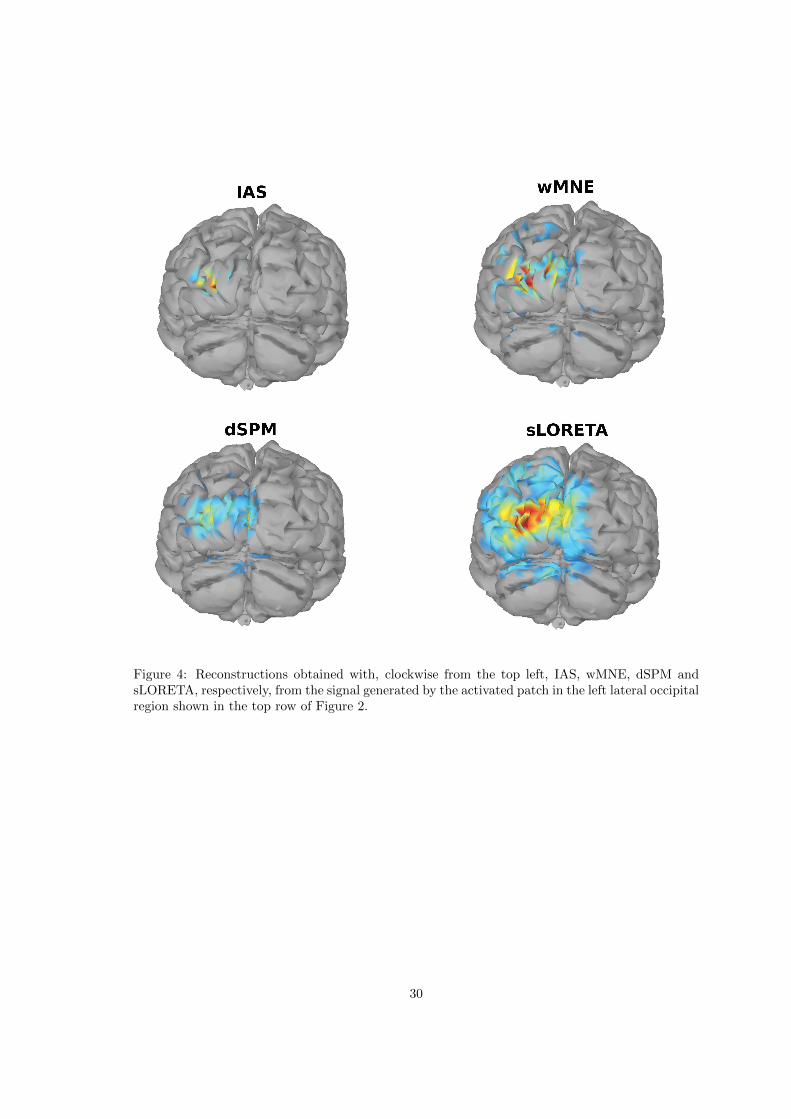
D. Calvetti REFERENCES
Figure 4
45
Figure 4: Reconstructions obtained with, clockwise from the top left, IAS, wMNE, dSPM andsLORETA, respectively, from the signal generated by the activated patch in the left lateral occipitalregion shown in the top row of Figure 2.
30

D. Calvetti REFERENCES
25 20 15 10 5 0 0 5 10 15 20 25
BANKSSTS
CAUDALANTERIORCINGULATE
CAUDALMIDDLEFRONTAL
CUNEUS
ENTORHINAL
FRONTALPOLE
FUSIFORM
INFERIORPARIETAL
INFERIORTEMPORAL
INSULA
ISTHMUSCINGULATE
LATERALOCCIPITAL
LATERALORBITOFRONTAL
LINGUAL
MEDIALORBITOFRONTAL
MIDDLETEMPORAL
PARACENTRAL
PARAHIPPOCAMPAL
PARSOPERCULARIS
PARSORBITALIS
PARSTRIANGULARIS
PERICALCARINE
POSTCENTRAL
POSTERIORCINGULATE
PRECENTRAL
PRECUNEUS
ROSTRALANTERIORCINGULATE
ROSTRALMIDDLEFRONTAL
SUPERIORFRONTAL
SUPERIORPARIETAL
SUPERIORTEMPORAL
SUPRAMARGINAL
TEMPORALPOLE
TRANSVERSETEMPORAL
ACCUMBENS
AMYGDALA
CAUDATE
CEREBELLUM
HIPPOCAMPUS
PALLIDUM
PUTAMEN
THALAMUS
BRAINSTEM
(a) IAS25 20 15 10 5 0 0 5 10 15 20 25
BANKSSTS
CAUDALANTERIORCINGULATE
CAUDALMIDDLEFRONTAL
CUNEUS
ENTORHINAL
FRONTALPOLE
FUSIFORM
INFERIORPARIETAL
INFERIORTEMPORAL
INSULA
ISTHMUSCINGULATE
LATERALOCCIPITAL
LATERALORBITOFRONTAL
LINGUAL
MEDIALORBITOFRONTAL
MIDDLETEMPORAL
PARACENTRAL
PARAHIPPOCAMPAL
PARSOPERCULARIS
PARSORBITALIS
PARSTRIANGULARIS
PERICALCARINE
POSTCENTRAL
POSTERIORCINGULATE
PRECENTRAL
PRECUNEUS
ROSTRALANTERIORCINGULATE
ROSTRALMIDDLEFRONTAL
SUPERIORFRONTAL
SUPERIORPARIETAL
SUPERIORTEMPORAL
SUPRAMARGINAL
TEMPORALPOLE
TRANSVERSETEMPORAL
ACCUMBENS
AMYGDALA
CAUDATE
CEREBELLUM
HIPPOCAMPUS
PALLIDUM
PUTAMEN
THALAMUS
BRAINSTEM
(b) wMNE
10 5 0 0 5 10
BANKSSTS
CAUDALANTERIORCINGULATE
CAUDALMIDDLEFRONTAL
CUNEUS
ENTORHINAL
FRONTALPOLE
FUSIFORM
INFERIORPARIETAL
INFERIORTEMPORAL
INSULA
ISTHMUSCINGULATE
LATERALOCCIPITAL
LATERALORBITOFRONTAL
LINGUAL
MEDIALORBITOFRONTAL
MIDDLETEMPORAL
PARACENTRAL
PARAHIPPOCAMPAL
PARSOPERCULARIS
PARSORBITALIS
PARSTRIANGULARIS
PERICALCARINE
POSTCENTRAL
POSTERIORCINGULATE
PRECENTRAL
PRECUNEUS
ROSTRALANTERIORCINGULATE
ROSTRALMIDDLEFRONTAL
SUPERIORFRONTAL
SUPERIORPARIETAL
SUPERIORTEMPORAL
SUPRAMARGINAL
TEMPORALPOLE
TRANSVERSETEMPORAL
ACCUMBENS
AMYGDALA
CAUDATE
CEREBELLUM
HIPPOCAMPUS
PALLIDUM
PUTAMEN
THALAMUS
BRAINSTEM
(c) dSPM10 5 0 0 5 10
BANKSSTS
CAUDALANTERIORCINGULATE
CAUDALMIDDLEFRONTAL
CUNEUS
ENTORHINAL
FRONTALPOLE
FUSIFORM
INFERIORPARIETAL
INFERIORTEMPORAL
INSULA
ISTHMUSCINGULATE
LATERALOCCIPITAL
LATERALORBITOFRONTAL
LINGUAL
MEDIALORBITOFRONTAL
MIDDLETEMPORAL
PARACENTRAL
PARAHIPPOCAMPAL
PARSOPERCULARIS
PARSORBITALIS
PARSTRIANGULARIS
PERICALCARINE
POSTCENTRAL
POSTERIORCINGULATE
PRECENTRAL
PRECUNEUS
ROSTRALANTERIORCINGULATE
ROSTRALMIDDLEFRONTAL
SUPERIORFRONTAL
SUPERIORPARIETAL
SUPERIORTEMPORAL
SUPRAMARGINAL
TEMPORALPOLE
TRANSVERSETEMPORAL
ACCUMBENS
AMYGDALA
CAUDATE
CEREBELLUM
HIPPOCAMPUS
PALLIDUM
PUTAMEN
THALAMUS
BRAINSTEM
(d) sLORETA
Figure 5
46
Figure 5: Mapping of the brain activity to 85 different BRs over 100 simulations using syntheticdata corresponding to randomly generated activity patches in the right cerebellum, indicated inred in the list of the BRs reconstructed with, respectively, IAS (a), wMNE (b), dSPM (c) andsLORETA (d). The histograms bin the average activity in each BR: in red the BRs of the lefthemisphere and in black the ones of the right hemisphere.
31

D. Calvetti REFERENCES
Figure 6
47
Figure 6: Reconstructions obtained with, clockwise from the top left, IAS, wMNE, dSPM andsLORETA, respectively, from the signal generated by the activated patch in the right cerebellumshown in the middle row of Figure 2.
32

D. Calvetti REFERENCES
(a) IAS (Left Hemisphere)
0
200
400
600
800
1000
1200
1400
1600
1800
2000
BANKSSTS
CAUDALANTERIO
RCIN
GULATE
CAUDALM
IDDLEFRONTAL
CUNEUS
ENTORHIN
AL
FRONTALPOLE
FUSIF
ORM
INFERIO
RPARIE
TAL
INFERIO
RTEM
PORAL
INSULA
ISTHM
USCIN
GULATE
LATERALOCCIP
ITAL
LATERALORBIT
OFRONTAL
LIN
GUAL
MEDIA
LORBIT
OFRONTAL
MID
DLETEM
PORAL
PARACENTRAL
PARAHIP
POCAM
PAL
PARSOPERCULARIS
PARSORBIT
ALIS
PARSTRIA
NGULARIS
PERIC
ALCARIN
E
POSTCENTRAL
POSTERIO
RCIN
GULATE
PRECENTRAL
PRECUNEUS
ROSTRALANTERIO
RCIN
GULATE
ROSTRALM
IDDLEFRONTAL
SUPERIO
RFRONTAL
SUPERIO
RPARIE
TAL
SUPERIO
RTEM
PORAL
SUPRAM
ARGIN
AL
TEM
PORALPOLE
TRANSVERSETEM
PORAL
(b) wMNE (Left Hemisphere
0
200
400
600
800
1000
1200
1400
1600
1800
2000
BANKSSTS
CAUDALANTERIO
RCIN
GULATE
CAUDALM
IDDLEFRONTAL
CUNEUS
ENTORHIN
AL
FRONTALPOLE
FUSIF
ORM
INFERIO
RPARIE
TAL
INFERIO
RTEM
PORAL
INSULA
ISTHM
USCIN
GULATE
LATERALOCCIP
ITAL
LATERALORBIT
OFRONTAL
LIN
GUAL
MEDIA
LORBIT
OFRONTAL
MID
DLETEM
PORAL
PARACENTRAL
PARAHIP
POCAM
PAL
PARSOPERCULARIS
PARSORBIT
ALIS
PARSTRIA
NGULARIS
PERIC
ALCARIN
E
POSTCENTRAL
POSTERIO
RCIN
GULATE
PRECENTRAL
PRECUNEUS
ROSTRALANTERIO
RCIN
GULATE
ROSTRALM
IDDLEFRONTAL
SUPERIO
RFRONTAL
SUPERIO
RPARIE
TAL
SUPERIO
RTEM
PORAL
SUPRAM
ARGIN
AL
TEM
PORALPOLE
TRANSVERSETEM
PORAL
0
200
400
600
800
1000
1200
1400
1600
1800
2000
ACCUM
BENS
AM
YGDALA
CAUDATE
CEREBELLUM
HIP
POCAM
PUS
PALLID
UM
PUTAM
EN
THALAM
US
0
200
400
600
800
1000
1200
1400
1600
1800
2000
ACCUM
BENS
AM
YGDALA
CAUDATE
CEREBELLUM
HIP
POCAM
PUS
PALLID
UM
PUTAM
EN
THALAM
US
BRAIN
STEM
Figure 7
48
Figure 7: Histograms of the Bayes factors for the cortical (top) and subcortical (bottom) BRs whenusing the IAS algorithm (left panel) and the wMNE algorithm (right panel) to map the MEG datato brain activity in the left hemisphere. Each histogram for each BR is the summary of 2000 Bayesfactor computations color coded to indicate the different level of support of the hypothesis: greenfor overwhelming support, blue for strong support, red for weak support, black no support.
33

D. Calvetti REFERENCES
(a) dSPM (Left Hemisphere)
0
200
400
600
800
1000
1200
1400
1600
1800
2000
BANKSSTS
CAUDALANTERIO
RCIN
GULATE
CAUDALM
IDDLEFRONTAL
CUNEUS
ENTORHIN
AL
FRONTALPOLE
FUSIF
ORM
INFERIO
RPARIE
TAL
INFERIO
RTEM
PORAL
INSULA
ISTHM
USCIN
GULATE
LATERALOCCIP
ITAL
LATERALORBIT
OFRONTAL
LIN
GUAL
MEDIA
LORBIT
OFRONTAL
MID
DLETEM
PORAL
PARACENTRAL
PARAHIP
POCAM
PAL
PARSOPERCULARIS
PARSORBIT
ALIS
PARSTRIA
NGULARIS
PERIC
ALCARIN
E
POSTCENTRAL
POSTERIO
RCIN
GULATE
PRECENTRAL
PRECUNEUS
ROSTRALANTERIO
RCIN
GULATE
ROSTRALM
IDDLEFRONTAL
SUPERIO
RFRONTAL
SUPERIO
RPARIE
TAL
SUPERIO
RTEM
PORAL
SUPRAM
ARGIN
AL
TEM
PORALPOLE
TRANSVERSETEM
PORAL
(b) sLORETA (Left Hemisphere)
0
200
400
600
800
1000
1200
1400
1600
1800
2000
BANKSSTS
CAUDALANTERIO
RCIN
GULATE
CAUDALM
IDDLEFRONTAL
CUNEUS
ENTORHIN
AL
FRONTALPOLE
FUSIF
ORM
INFERIO
RPARIE
TAL
INFERIO
RTEM
PORAL
INSULA
ISTHM
USCIN
GULATE
LATERALOCCIP
ITAL
LATERALORBIT
OFRONTAL
LIN
GUAL
MEDIA
LORBIT
OFRONTAL
MID
DLETEM
PORAL
PARACENTRAL
PARAHIP
POCAM
PAL
PARSOPERCULARIS
PARSORBIT
ALIS
PARSTRIA
NGULARIS
PERIC
ALCARIN
E
POSTCENTRAL
POSTERIO
RCIN
GULATE
PRECENTRAL
PRECUNEUS
ROSTRALANTERIO
RCIN
GULATE
ROSTRALM
IDDLEFRONTAL
SUPERIO
RFRONTAL
SUPERIO
RPARIE
TAL
SUPERIO
RTEM
PORAL
SUPRAM
ARGIN
AL
TEM
PORALPOLE
TRANSVERSETEM
PORAL
0
200
400
600
800
1000
1200
1400
1600
1800
2000
ACCUM
BENS
AM
YGDALA
CAUDATE
CEREBELLUM
HIP
POCAM
PUS
PALLID
UM
PUTAM
EN
THALAM
US
0
200
400
600
800
1000
1200
1400
1600
1800
2000
ACCUM
BENS
AM
YGDALA
CAUDATE
CEREBELLUM
HIP
POCAM
PUS
PALLID
UM
PUTAM
EN
THALAM
US
Figure 8
49
Figure 8: Histograms of the Bayes factors for the cortical (top) and subcortical (bottom) BRswhen using the dSPM algorithm (left panel) and the sLORETA algorithm (right panel)to map theMEG data to brain activity in the left hemisphere. Each histogram for each BR is the summaryof 2000 Bayes factor computations and the color coding is as explained in Figure 7.
34

D. Calvetti REFERENCES
0
200
400
600
800
1000
1200
1400
1600
1800
2000
IAS
wM
NE
dSPM
sLore
ta
AMYGDALA
0
200
400
600
800
1000
1200
1400
1600
1800
2000
IAS
wM
NE
dSPM
sLore
ta
FRONTALPOLE
0
200
400
600
800
1000
1200
1400
1600
1800
2000
IAS
wM
NE
dSPM
sLore
ta
CEREBELLUM
0
200
400
600
800
1000
1200
1400
1600
1800
2000
IAS
wM
NE
dSPM
sLore
ta
PRECENTRAL
0
200
400
600
800
1000
1200
1400
1600
1800
2000
IAS
wM
NE
dSPM
sLore
ta
PRECENTRAL
0
200
400
600
800
1000
1200
1400
1600
1800
2000
IAS
wM
NE
dSPM
sLore
ta
HIPPOCAMPUS
0
200
400
600
800
1000
1200
1400
1600
1800
2000
IAS
wM
NE
dSPM
sLore
ta
THALAMUS
0
200
400
600
800
1000
1200
1400
1600
1800
2000
IAS
wM
NE
dSPM
sLore
ta
INFERIORPARIETAL L
0
200
400
600
800
1000
1200
1400
1600
1800
2000
IAS
wM
NE
dSPM
sLore
ta
PRECUNEUS L
0
200
400
600
800
1000
1200
1400
1600
1800
2000
IAS
wM
NE
dSPM
sLore
ta
CAUDALANTERIORCINGULATE L
0
200
400
600
800
1000
1200
1400
1600
1800
2000
IAS
wM
NE
dSPM
sLore
ta
INFERIORPARIETAL R
0
200
400
600
800
1000
1200
1400
1600
1800
2000
IAS
wM
NE
dSPM
sLore
ta
PRECUNEUS R
0
200
400
600
800
1000
1200
1400
1600
1800
2000
IAS
wM
NE
dSPM
sLore
ta
CAUDALANTERIORCINGULATE R
Figure 9
50Figure 9: Row-wise from top to bottom: Row 1: Bayes factors in the case of two active patches.Left panel: Bayes factors in support of the hypothesis that the activity is in the left amygdalawhen the data comes from two active patches, one in the left amygdala and the other in the leftfrontal pole, and the MEG inverse problem is solved with the IAS, wMNE, dSPM and sLORETAalgorithms, respectively. The histograms where computed from 2000 realizations and the colorcoding is as explained in Figure 7. Right panel: Bayes factors in support of activity in the leftfrontal pole computed from the same 2000 realizations. Row 2: Bayes factors in the case of twoactive patches. Left panel: Bayes factors in support of the hypothesis that the activity is in the leftcerebellum when the data comes from two active patches, one in the left cerebellum and the otherin the left precentral cortex, and the MEG inverse problem is solved with the IAS, wMNE, dSPMand sLORETA algorithms, respectively. The histograms were computed from 2000 realizationsRight panel: Bayes factors in support of activity in the left precentral cortex computed from thesame 2000 realizations. Row 3: Bayes factors in the case of active patches in three different BRs,the right precentral gyrus (left), and the left hippocampus (center) and the right thalamus (right),and the MEG inverse problem is solved with the IAS, wMNE, dSPM and sLORETA algorithms,respectively. The histograms were computed from 2000 realizations. Rows 5-6: Bayes factorsfor the case where there are active patches in all six BRs comprising the Default Mode Network:inferior parietal gyrus, precuneus and caudal anterior cingulate gyrus in the left (top) and right(bottom) hemispheres to test the specificity of the IAS inverse solver and the three reference inversesolvers.
35

D. Calvetti REFERENCES
15 10 5 0 0 5 10 15
BANKSSTS
CAUDALANTERIORCINGULATE
CAUDALMIDDLEFRONTAL
CUNEUS
ENTORHINAL
FRONTALPOLE
FUSIFORM
INFERIORPARIETAL
INFERIORTEMPORAL
INSULA
ISTHMUSCINGULATE
LATERALOCCIPITAL
LATERALORBITOFRONTAL
LINGUAL
MEDIALORBITOFRONTAL
MIDDLETEMPORAL
PARACENTRAL
PARAHIPPOCAMPAL
PARSOPERCULARIS
PARSORBITALIS
PARSTRIANGULARIS
PERICALCARINE
POSTCENTRAL
POSTERIORCINGULATE
PRECENTRAL
PRECUNEUS
ROSTRALANTERIORCINGULATE
ROSTRALMIDDLEFRONTAL
SUPERIORFRONTAL
SUPERIORPARIETAL
SUPERIORTEMPORAL
SUPRAMARGINAL
TEMPORALPOLE
TRANSVERSETEMPORAL
ACCUMBENS
AMYGDALA
CAUDATE
CEREBELLUM
HIPPOCAMPUS
PALLIDUM
PUTAMEN
THALAMUS
BRAINSTEM
(a) IAS15 10 5 0 0 5 10 15
BANKSSTS
CAUDALANTERIORCINGULATE
CAUDALMIDDLEFRONTAL
CUNEUS
ENTORHINAL
FRONTALPOLE
FUSIFORM
INFERIORPARIETAL
INFERIORTEMPORAL
INSULA
ISTHMUSCINGULATE
LATERALOCCIPITAL
LATERALORBITOFRONTAL
LINGUAL
MEDIALORBITOFRONTAL
MIDDLETEMPORAL
PARACENTRAL
PARAHIPPOCAMPAL
PARSOPERCULARIS
PARSORBITALIS
PARSTRIANGULARIS
PERICALCARINE
POSTCENTRAL
POSTERIORCINGULATE
PRECENTRAL
PRECUNEUS
ROSTRALANTERIORCINGULATE
ROSTRALMIDDLEFRONTAL
SUPERIORFRONTAL
SUPERIORPARIETAL
SUPERIORTEMPORAL
SUPRAMARGINAL
TEMPORALPOLE
TRANSVERSETEMPORAL
ACCUMBENS
AMYGDALA
CAUDATE
CEREBELLUM
HIPPOCAMPUS
PALLIDUM
PUTAMEN
THALAMUS
BRAINSTEM
(b) wMNE
15 10 5 0 0 5 10 15
BANKSSTS
CAUDALANTERIORCINGULATE
CAUDALMIDDLEFRONTAL
CUNEUS
ENTORHINAL
FRONTALPOLE
FUSIFORM
INFERIORPARIETAL
INFERIORTEMPORAL
INSULA
ISTHMUSCINGULATE
LATERALOCCIPITAL
LATERALORBITOFRONTAL
LINGUAL
MEDIALORBITOFRONTAL
MIDDLETEMPORAL
PARACENTRAL
PARAHIPPOCAMPAL
PARSOPERCULARIS
PARSORBITALIS
PARSTRIANGULARIS
PERICALCARINE
POSTCENTRAL
POSTERIORCINGULATE
PRECENTRAL
PRECUNEUS
ROSTRALANTERIORCINGULATE
ROSTRALMIDDLEFRONTAL
SUPERIORFRONTAL
SUPERIORPARIETAL
SUPERIORTEMPORAL
SUPRAMARGINAL
TEMPORALPOLE
TRANSVERSETEMPORAL
ACCUMBENS
AMYGDALA
CAUDATE
CEREBELLUM
HIPPOCAMPUS
PALLIDUM
PUTAMEN
THALAMUS
BRAINSTEM
(c) dSPM15 10 5 0 0 5 10 15
BANKSSTS
CAUDALANTERIORCINGULATE
CAUDALMIDDLEFRONTAL
CUNEUS
ENTORHINAL
FRONTALPOLE
FUSIFORM
INFERIORPARIETAL
INFERIORTEMPORAL
INSULA
ISTHMUSCINGULATE
LATERALOCCIPITAL
LATERALORBITOFRONTAL
LINGUAL
MEDIALORBITOFRONTAL
MIDDLETEMPORAL
PARACENTRAL
PARAHIPPOCAMPAL
PARSOPERCULARIS
PARSORBITALIS
PARSTRIANGULARIS
PERICALCARINE
POSTCENTRAL
POSTERIORCINGULATE
PRECENTRAL
PRECUNEUS
ROSTRALANTERIORCINGULATE
ROSTRALMIDDLEFRONTAL
SUPERIORFRONTAL
SUPERIORPARIETAL
SUPERIORTEMPORAL
SUPRAMARGINAL
TEMPORALPOLE
TRANSVERSETEMPORAL
ACCUMBENS
AMYGDALA
CAUDATE
CEREBELLUM
HIPPOCAMPUS
PALLIDUM
PUTAMEN
THALAMUS
BRAINSTEM
(d) sLORETA
Figure 10
51
Figure 10: Mapping of the brain activity to 85 different BRs for the time T = 5 ms withreal/realistic data example reconstructed with, respectively, IAS (a), wMNE (b), dSPM (c) andsLORETA (d). The histograms bin the average activity in each BR: in red the BRs of the lefthemisphere and in black the ones of the right hemisphere.
36

D. Calvetti REFERENCES
15 10 5 0 0 5 10 15
BANKSSTS
CAUDALANTERIORCINGULATE
CAUDALMIDDLEFRONTAL
CUNEUS
ENTORHINAL
FRONTALPOLE
FUSIFORM
INFERIORPARIETAL
INFERIORTEMPORAL
INSULA
ISTHMUSCINGULATE
LATERALOCCIPITAL
LATERALORBITOFRONTAL
LINGUAL
MEDIALORBITOFRONTAL
MIDDLETEMPORAL
PARACENTRAL
PARAHIPPOCAMPAL
PARSOPERCULARIS
PARSORBITALIS
PARSTRIANGULARIS
PERICALCARINE
POSTCENTRAL
POSTERIORCINGULATE
PRECENTRAL
PRECUNEUS
ROSTRALANTERIORCINGULATE
ROSTRALMIDDLEFRONTAL
SUPERIORFRONTAL
SUPERIORPARIETAL
SUPERIORTEMPORAL
SUPRAMARGINAL
TEMPORALPOLE
TRANSVERSETEMPORAL
ACCUMBENS
AMYGDALA
CAUDATE
CEREBELLUM
HIPPOCAMPUS
PALLIDUM
PUTAMEN
THALAMUS
BRAINSTEM
(a) IAS15 10 5 0 0 5 10 15
BANKSSTS
CAUDALANTERIORCINGULATE
CAUDALMIDDLEFRONTAL
CUNEUS
ENTORHINAL
FRONTALPOLE
FUSIFORM
INFERIORPARIETAL
INFERIORTEMPORAL
INSULA
ISTHMUSCINGULATE
LATERALOCCIPITAL
LATERALORBITOFRONTAL
LINGUAL
MEDIALORBITOFRONTAL
MIDDLETEMPORAL
PARACENTRAL
PARAHIPPOCAMPAL
PARSOPERCULARIS
PARSORBITALIS
PARSTRIANGULARIS
PERICALCARINE
POSTCENTRAL
POSTERIORCINGULATE
PRECENTRAL
PRECUNEUS
ROSTRALANTERIORCINGULATE
ROSTRALMIDDLEFRONTAL
SUPERIORFRONTAL
SUPERIORPARIETAL
SUPERIORTEMPORAL
SUPRAMARGINAL
TEMPORALPOLE
TRANSVERSETEMPORAL
ACCUMBENS
AMYGDALA
CAUDATE
CEREBELLUM
HIPPOCAMPUS
PALLIDUM
PUTAMEN
THALAMUS
BRAINSTEM
(b) wMNE
15 10 5 0 0 5 10 15
BANKSSTS
CAUDALANTERIORCINGULATE
CAUDALMIDDLEFRONTAL
CUNEUS
ENTORHINAL
FRONTALPOLE
FUSIFORM
INFERIORPARIETAL
INFERIORTEMPORAL
INSULA
ISTHMUSCINGULATE
LATERALOCCIPITAL
LATERALORBITOFRONTAL
LINGUAL
MEDIALORBITOFRONTAL
MIDDLETEMPORAL
PARACENTRAL
PARAHIPPOCAMPAL
PARSOPERCULARIS
PARSORBITALIS
PARSTRIANGULARIS
PERICALCARINE
POSTCENTRAL
POSTERIORCINGULATE
PRECENTRAL
PRECUNEUS
ROSTRALANTERIORCINGULATE
ROSTRALMIDDLEFRONTAL
SUPERIORFRONTAL
SUPERIORPARIETAL
SUPERIORTEMPORAL
SUPRAMARGINAL
TEMPORALPOLE
TRANSVERSETEMPORAL
ACCUMBENS
AMYGDALA
CAUDATE
CEREBELLUM
HIPPOCAMPUS
PALLIDUM
PUTAMEN
THALAMUS
BRAINSTEM
(c) dSPM15 10 5 0 0 5 10 15
BANKSSTS
CAUDALANTERIORCINGULATE
CAUDALMIDDLEFRONTAL
CUNEUS
ENTORHINAL
FRONTALPOLE
FUSIFORM
INFERIORPARIETAL
INFERIORTEMPORAL
INSULA
ISTHMUSCINGULATE
LATERALOCCIPITAL
LATERALORBITOFRONTAL
LINGUAL
MEDIALORBITOFRONTAL
MIDDLETEMPORAL
PARACENTRAL
PARAHIPPOCAMPAL
PARSOPERCULARIS
PARSORBITALIS
PARSTRIANGULARIS
PERICALCARINE
POSTCENTRAL
POSTERIORCINGULATE
PRECENTRAL
PRECUNEUS
ROSTRALANTERIORCINGULATE
ROSTRALMIDDLEFRONTAL
SUPERIORFRONTAL
SUPERIORPARIETAL
SUPERIORTEMPORAL
SUPRAMARGINAL
TEMPORALPOLE
TRANSVERSETEMPORAL
ACCUMBENS
AMYGDALA
CAUDATE
CEREBELLUM
HIPPOCAMPUS
PALLIDUM
PUTAMEN
THALAMUS
BRAINSTEM
(d) sLORETA
Figure 11
52
Figure 11: Mapping of the brain activity to 85 different BRs for the time T = 100 ms withreal/realistic data example reconstructed with, respectively, IAS (a), wMNE (b), dSPM (c) andsLORETA (d). The histograms bin the average activity in each BR: in red the BRs of the lefthemisphere and in black the ones of the right hemisphere.
37
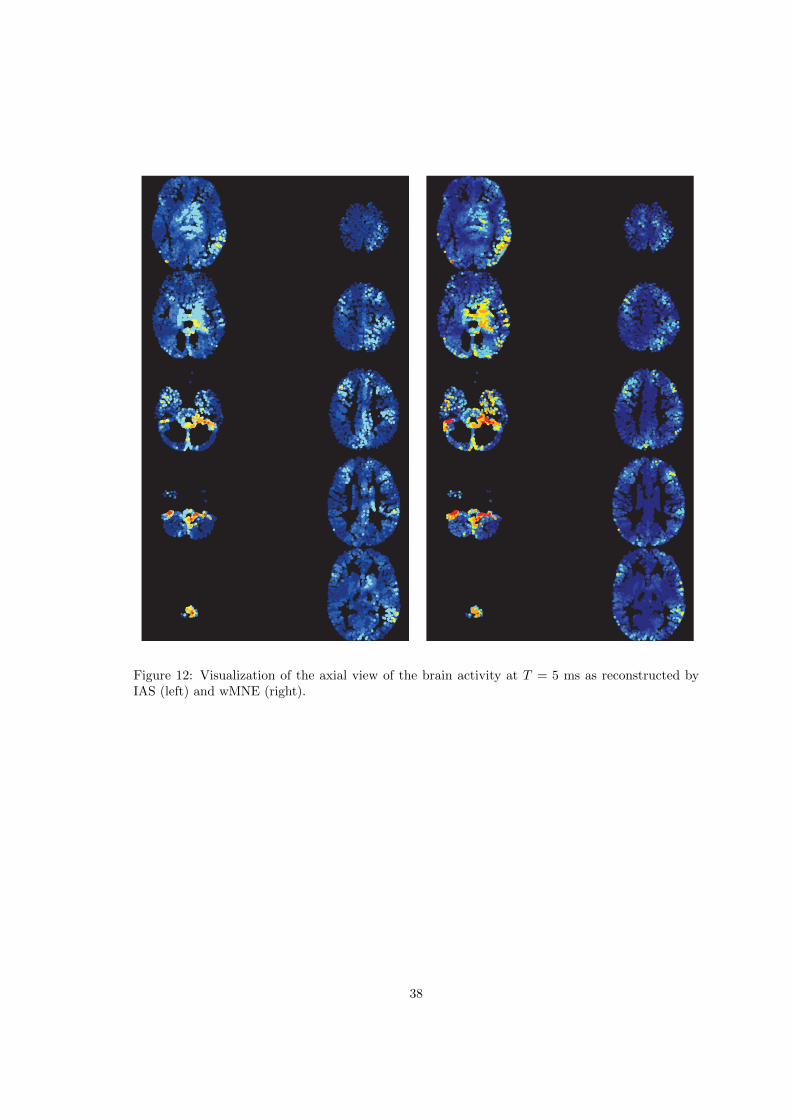
D. Calvetti REFERENCES
Figure 12
53
Figure 12: Visualization of the axial view of the brain activity at T = 5 ms as reconstructed byIAS (left) and wMNE (right).
38

D. Calvetti REFERENCES
Figure 13
54
Figure 13: Visualization of the axial view of the brain activity at T = 5 ms as reconstructed bydSPM (left) and sLORETA (right).
39

D. Calvetti REFERENCES
Figure 14
55
Figure 14: Reconstructions obtained from real data at time T = 5 ms with, top to bottom, IAS,wMNE, dSPM and sLORETA, respectively. At this time instant, most of the signal is generatedby the patch activity in the brainstem shown in the bottom row of Figure 2.
40

D. Calvetti REFERENCES
Figure 15
56
Figure 15: Visualization of the axial view of the brain activity at T = 100 ms as reconstructed byIAS (left) and wMNE (right).
41

D. Calvetti REFERENCES
Figure 16
57
Figure 16: Visualization of the axial view of the brain activity at T = 100 ms as reconstructed bydSPM (left) and sLORETA (right).
42

D. Calvetti REFERENCES
Figure 17
58
Figure 17: Reconstructions obtained from real data at time T = 100 ms with, top to bottom, IAS,wMNE, dSPM and sLORETA, respectively.
43

Supplementary material
44
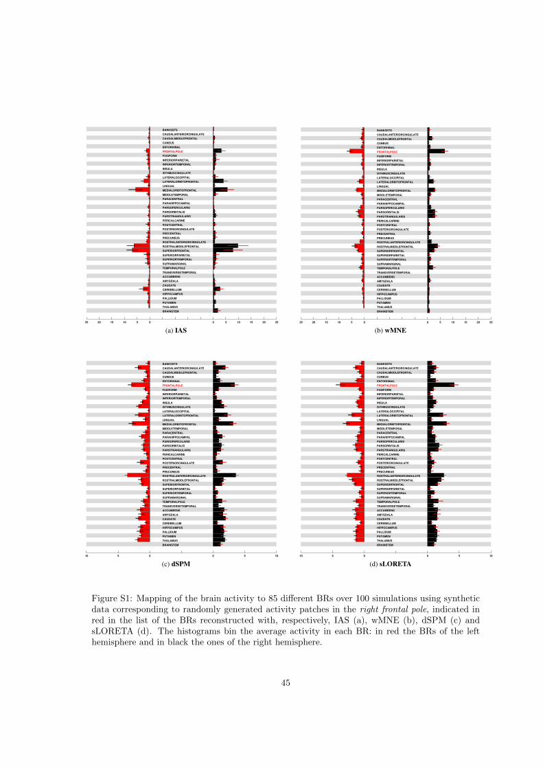
D. Calvetti REFERENCES
25 20 15 10 5 0 0 5 10 15 20 25
BANKSSTS
CAUDALANTERIORCINGULATE
CAUDALMIDDLEFRONTAL
CUNEUS
ENTORHINAL
FRONTALPOLE
FUSIFORM
INFERIORPARIETAL
INFERIORTEMPORAL
INSULA
ISTHMUSCINGULATE
LATERALOCCIPITAL
LATERALORBITOFRONTAL
LINGUAL
MEDIALORBITOFRONTAL
MIDDLETEMPORAL
PARACENTRAL
PARAHIPPOCAMPAL
PARSOPERCULARIS
PARSORBITALIS
PARSTRIANGULARIS
PERICALCARINE
POSTCENTRAL
POSTERIORCINGULATE
PRECENTRAL
PRECUNEUS
ROSTRALANTERIORCINGULATE
ROSTRALMIDDLEFRONTAL
SUPERIORFRONTAL
SUPERIORPARIETAL
SUPERIORTEMPORAL
SUPRAMARGINAL
TEMPORALPOLE
TRANSVERSETEMPORAL
ACCUMBENS
AMYGDALA
CAUDATE
CEREBELLUM
HIPPOCAMPUS
PALLIDUM
PUTAMEN
THALAMUS
BRAINSTEM
FRONTALPOLE R
(a) IAS25 20 15 10 5 0 0 5 10 15 20 25
BANKSSTS
CAUDALANTERIORCINGULATE
CAUDALMIDDLEFRONTAL
CUNEUS
ENTORHINAL
FRONTALPOLE
FUSIFORM
INFERIORPARIETAL
INFERIORTEMPORAL
INSULA
ISTHMUSCINGULATE
LATERALOCCIPITAL
LATERALORBITOFRONTAL
LINGUAL
MEDIALORBITOFRONTAL
MIDDLETEMPORAL
PARACENTRAL
PARAHIPPOCAMPAL
PARSOPERCULARIS
PARSORBITALIS
PARSTRIANGULARIS
PERICALCARINE
POSTCENTRAL
POSTERIORCINGULATE
PRECENTRAL
PRECUNEUS
ROSTRALANTERIORCINGULATE
ROSTRALMIDDLEFRONTAL
SUPERIORFRONTAL
SUPERIORPARIETAL
SUPERIORTEMPORAL
SUPRAMARGINAL
TEMPORALPOLE
TRANSVERSETEMPORAL
ACCUMBENS
AMYGDALA
CAUDATE
CEREBELLUM
HIPPOCAMPUS
PALLIDUM
PUTAMEN
THALAMUS
BRAINSTEM
(b) wMNE
10 5 0 0 5 10
BANKSSTS
CAUDALANTERIORCINGULATE
CAUDALMIDDLEFRONTAL
CUNEUS
ENTORHINAL
FRONTALPOLE
FUSIFORM
INFERIORPARIETAL
INFERIORTEMPORAL
INSULA
ISTHMUSCINGULATE
LATERALOCCIPITAL
LATERALORBITOFRONTAL
LINGUAL
MEDIALORBITOFRONTAL
MIDDLETEMPORAL
PARACENTRAL
PARAHIPPOCAMPAL
PARSOPERCULARIS
PARSORBITALIS
PARSTRIANGULARIS
PERICALCARINE
POSTCENTRAL
POSTERIORCINGULATE
PRECENTRAL
PRECUNEUS
ROSTRALANTERIORCINGULATE
ROSTRALMIDDLEFRONTAL
SUPERIORFRONTAL
SUPERIORPARIETAL
SUPERIORTEMPORAL
SUPRAMARGINAL
TEMPORALPOLE
TRANSVERSETEMPORAL
ACCUMBENS
AMYGDALA
CAUDATE
CEREBELLUM
HIPPOCAMPUS
PALLIDUM
PUTAMEN
THALAMUS
BRAINSTEM
(c) dSPM10 5 0 0 5 10
BANKSSTS
CAUDALANTERIORCINGULATE
CAUDALMIDDLEFRONTAL
CUNEUS
ENTORHINAL
FRONTALPOLE
FUSIFORM
INFERIORPARIETAL
INFERIORTEMPORAL
INSULA
ISTHMUSCINGULATE
LATERALOCCIPITAL
LATERALORBITOFRONTAL
LINGUAL
MEDIALORBITOFRONTAL
MIDDLETEMPORAL
PARACENTRAL
PARAHIPPOCAMPAL
PARSOPERCULARIS
PARSORBITALIS
PARSTRIANGULARIS
PERICALCARINE
POSTCENTRAL
POSTERIORCINGULATE
PRECENTRAL
PRECUNEUS
ROSTRALANTERIORCINGULATE
ROSTRALMIDDLEFRONTAL
SUPERIORFRONTAL
SUPERIORPARIETAL
SUPERIORTEMPORAL
SUPRAMARGINAL
TEMPORALPOLE
TRANSVERSETEMPORAL
ACCUMBENS
AMYGDALA
CAUDATE
CEREBELLUM
HIPPOCAMPUS
PALLIDUM
PUTAMEN
THALAMUS
BRAINSTEM
(d) sLORETA
Figure S1
61
Figure S1: Mapping of the brain activity to 85 different BRs over 100 simulations using syntheticdata corresponding to randomly generated activity patches in the right frontal pole, indicated inred in the list of the BRs reconstructed with, respectively, IAS (a), wMNE (b), dSPM (c) andsLORETA (d). The histograms bin the average activity in each BR: in red the BRs of the lefthemisphere and in black the ones of the right hemisphere.
45
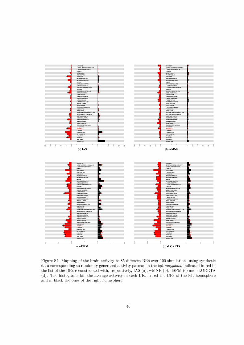
D. Calvetti REFERENCES
25 20 15 10 5 0 0 5 10 15 20 25
BANKSSTS
CAUDALANTERIORCINGULATE
CAUDALMIDDLEFRONTAL
CUNEUS
ENTORHINAL
FRONTALPOLE
FUSIFORM
INFERIORPARIETAL
INFERIORTEMPORAL
INSULA
ISTHMUSCINGULATE
LATERALOCCIPITAL
LATERALORBITOFRONTAL
LINGUAL
MEDIALORBITOFRONTAL
MIDDLETEMPORAL
PARACENTRAL
PARAHIPPOCAMPAL
PARSOPERCULARIS
PARSORBITALIS
PARSTRIANGULARIS
PERICALCARINE
POSTCENTRAL
POSTERIORCINGULATE
PRECENTRAL
PRECUNEUS
ROSTRALANTERIORCINGULATE
ROSTRALMIDDLEFRONTAL
SUPERIORFRONTAL
SUPERIORPARIETAL
SUPERIORTEMPORAL
SUPRAMARGINAL
TEMPORALPOLE
TRANSVERSETEMPORAL
ACCUMBENS
AMYGDALA
CAUDATE
CEREBELLUM
HIPPOCAMPUS
PALLIDUM
PUTAMEN
THALAMUS
BRAINSTEM
AMYGDALA L
(a) IAS25 20 15 10 5 0 0 5 10 15 20 25
BANKSSTS
CAUDALANTERIORCINGULATE
CAUDALMIDDLEFRONTAL
CUNEUS
ENTORHINAL
FRONTALPOLE
FUSIFORM
INFERIORPARIETAL
INFERIORTEMPORAL
INSULA
ISTHMUSCINGULATE
LATERALOCCIPITAL
LATERALORBITOFRONTAL
LINGUAL
MEDIALORBITOFRONTAL
MIDDLETEMPORAL
PARACENTRAL
PARAHIPPOCAMPAL
PARSOPERCULARIS
PARSORBITALIS
PARSTRIANGULARIS
PERICALCARINE
POSTCENTRAL
POSTERIORCINGULATE
PRECENTRAL
PRECUNEUS
ROSTRALANTERIORCINGULATE
ROSTRALMIDDLEFRONTAL
SUPERIORFRONTAL
SUPERIORPARIETAL
SUPERIORTEMPORAL
SUPRAMARGINAL
TEMPORALPOLE
TRANSVERSETEMPORAL
ACCUMBENS
AMYGDALA
CAUDATE
CEREBELLUM
HIPPOCAMPUS
PALLIDUM
PUTAMEN
THALAMUS
BRAINSTEM
(b) wMNE
10 5 0 0 5 10
BANKSSTS
CAUDALANTERIORCINGULATE
CAUDALMIDDLEFRONTAL
CUNEUS
ENTORHINAL
FRONTALPOLE
FUSIFORM
INFERIORPARIETAL
INFERIORTEMPORAL
INSULA
ISTHMUSCINGULATE
LATERALOCCIPITAL
LATERALORBITOFRONTAL
LINGUAL
MEDIALORBITOFRONTAL
MIDDLETEMPORAL
PARACENTRAL
PARAHIPPOCAMPAL
PARSOPERCULARIS
PARSORBITALIS
PARSTRIANGULARIS
PERICALCARINE
POSTCENTRAL
POSTERIORCINGULATE
PRECENTRAL
PRECUNEUS
ROSTRALANTERIORCINGULATE
ROSTRALMIDDLEFRONTAL
SUPERIORFRONTAL
SUPERIORPARIETAL
SUPERIORTEMPORAL
SUPRAMARGINAL
TEMPORALPOLE
TRANSVERSETEMPORAL
ACCUMBENS
AMYGDALA
CAUDATE
CEREBELLUM
HIPPOCAMPUS
PALLIDUM
PUTAMEN
THALAMUS
BRAINSTEM
(c) dSPM10 5 0 0 5 10
BANKSSTS
CAUDALANTERIORCINGULATE
CAUDALMIDDLEFRONTAL
CUNEUS
ENTORHINAL
FRONTALPOLE
FUSIFORM
INFERIORPARIETAL
INFERIORTEMPORAL
INSULA
ISTHMUSCINGULATE
LATERALOCCIPITAL
LATERALORBITOFRONTAL
LINGUAL
MEDIALORBITOFRONTAL
MIDDLETEMPORAL
PARACENTRAL
PARAHIPPOCAMPAL
PARSOPERCULARIS
PARSORBITALIS
PARSTRIANGULARIS
PERICALCARINE
POSTCENTRAL
POSTERIORCINGULATE
PRECENTRAL
PRECUNEUS
ROSTRALANTERIORCINGULATE
ROSTRALMIDDLEFRONTAL
SUPERIORFRONTAL
SUPERIORPARIETAL
SUPERIORTEMPORAL
SUPRAMARGINAL
TEMPORALPOLE
TRANSVERSETEMPORAL
ACCUMBENS
AMYGDALA
CAUDATE
CEREBELLUM
HIPPOCAMPUS
PALLIDUM
PUTAMEN
THALAMUS
BRAINSTEM
(d) sLORETA
Figure S2
62
Figure S2: Mapping of the brain activity to 85 different BRs over 100 simulations using syntheticdata corresponding to randomly generated activity patches in the left amygdala, indicated in red inthe list of the BRs reconstructed with, respectively, IAS (a), wMNE (b), dSPM (c) and sLORETA(d). The histograms bin the average activity in each BR: in red the BRs of the left hemisphereand in black the ones of the right hemisphere.
46