bqcd manual - universität hamburg · programming language. . . . . . . . . . . . . . . . . . . . ....
TRANSCRIPT

BQCD Manual
T.R. Haar, Y. Nakamura and H. Stuben
June 2017

Authors
Taylor Ryan HaarCSSM, Department of PhysicsThe University of AdelaideAdelaide, SAAustralia 5005
Yoshifumi NakamuraRIKEN Advanced Institute for Computational ScienceKobe, Hyogo 650-0047Japan
Hinnerk StubenUniversitat HamburgRegionales Rechenzentrum20146 HamburgGermany
Copyright c© 2017 Taylor Ryan Haar, Yoshifumi Nakamura, Hinnerk Stuben
$Id: svn_id.tex 989 2017-06-20 07:19:40Z rzxa001 $
2
Contents
Contents
Preface 7
1. Overview 81.1. Summary of changes . . . . . . . . . . . . . . . . . . . . . . . . . . . . . 9
2. Installation 102.1. Prerequisites . . . . . . . . . . . . . . . . . . . . . . . . . . . . . . . . . . 10
2.1.1. lime . . . . . . . . . . . . . . . . . . . . . . . . . . . . . . . . . . 102.1.2. LAPACK and ScaLAPACK . . . . . . . . . . . . . . . . . . . . . 10
2.2. Download . . . . . . . . . . . . . . . . . . . . . . . . . . . . . . . . . . . 112.3. License . . . . . . . . . . . . . . . . . . . . . . . . . . . . . . . . . . . . . 112.4. Configuration . . . . . . . . . . . . . . . . . . . . . . . . . . . . . . . . . 11
2.4.1. Supported platforms . . . . . . . . . . . . . . . . . . . . . . . . . 112.4.2. Settings in Makefile.var . . . . . . . . . . . . . . . . . . . . . . 122.4.3. Configuring/porting SIMD . . . . . . . . . . . . . . . . . . . . . . 12
2.5. Testing . . . . . . . . . . . . . . . . . . . . . . . . . . . . . . . . . . . . . 12
3. Usage 143.1. Quickstart guide . . . . . . . . . . . . . . . . . . . . . . . . . . . . . . . 14
3.1.1. Basics . . . . . . . . . . . . . . . . . . . . . . . . . . . . . . . . . 143.1.2. Gauge and fermion fields . . . . . . . . . . . . . . . . . . . . . . . 143.1.3. Molecular dynamics . . . . . . . . . . . . . . . . . . . . . . . . . . 153.1.4. Markov Chain . . . . . . . . . . . . . . . . . . . . . . . . . . . . . 163.1.5. Fermion matrix inversion . . . . . . . . . . . . . . . . . . . . . . . 163.1.6. Running BQCD . . . . . . . . . . . . . . . . . . . . . . . . . . . . 173.1.7. BQCD output . . . . . . . . . . . . . . . . . . . . . . . . . . . . . 17
3.2. Command line . . . . . . . . . . . . . . . . . . . . . . . . . . . . . . . . . 193.2.1. Flag -c (continuation job) . . . . . . . . . . . . . . . . . . . . . . 193.2.2. Flag --convert-to-ildg . . . . . . . . . . . . . . . . . . . . . . 193.2.3. Flag -I (print default input values) . . . . . . . . . . . . . . . . . 193.2.4. Flag -V (print program version) . . . . . . . . . . . . . . . . . . . 193.2.5. Argument input . . . . . . . . . . . . . . . . . . . . . . . . . . . 203.2.6. Argument output . . . . . . . . . . . . . . . . . . . . . . . . . . 20
3.3. Input parameters and the syntax of input file . . . . . . . . . . . . . . . 203.3.1. General parameters . . . . . . . . . . . . . . . . . . . . . . . . . . 203.3.2. Lattice and domain decomposition . . . . . . . . . . . . . . . . . 213.3.3. Gauge action . . . . . . . . . . . . . . . . . . . . . . . . . . . . . 223.3.4. Fermion action . . . . . . . . . . . . . . . . . . . . . . . . . . . . 223.3.5. Double-flavour pseudofermions . . . . . . . . . . . . . . . . . . . . 243.3.6. Single-flavour pseudofermions . . . . . . . . . . . . . . . . . . . . 253.3.7. RHMC tuning parameters . . . . . . . . . . . . . . . . . . . . . . 26
3
Contents
3.3.8. Zolotarev rational approximation . . . . . . . . . . . . . . . . . . 263.3.9. QED . . . . . . . . . . . . . . . . . . . . . . . . . . . . . . . . . . 273.3.10. Axion . . . . . . . . . . . . . . . . . . . . . . . . . . . . . . . . . 273.3.11. PFHMC . . . . . . . . . . . . . . . . . . . . . . . . . . . . . . . . 283.3.12. Truncated rational HMC (tRHMC) . . . . . . . . . . . . . . . . 303.3.13. Start parameters . . . . . . . . . . . . . . . . . . . . . . . . . . . 303.3.14. Configuration I/O . . . . . . . . . . . . . . . . . . . . . . . . . . . 313.3.15. Markov Chain . . . . . . . . . . . . . . . . . . . . . . . . . . . . . 333.3.16. Hybrid Monte Carlo . . . . . . . . . . . . . . . . . . . . . . . . . 343.3.17. Integrator specification . . . . . . . . . . . . . . . . . . . . . . . . 343.3.18. Time scale specifiers . . . . . . . . . . . . . . . . . . . . . . . . . 363.3.19. Solver parameters . . . . . . . . . . . . . . . . . . . . . . . . . . . 373.3.20. Measurements . . . . . . . . . . . . . . . . . . . . . . . . . . . . . 393.3.21. Compute performance tuning . . . . . . . . . . . . . . . . . . . . 423.3.22. Miscellaneous . . . . . . . . . . . . . . . . . . . . . . . . . . . . . 44
3.4. File naming conventions . . . . . . . . . . . . . . . . . . . . . . . . . . . 443.4.1. input, output and batch log files . . . . . . . . . . . . . . . . . . 453.4.2. Restart files in bqcd format . . . . . . . . . . . . . . . . . . . . . 453.4.3. Restart files in bqcd2 format . . . . . . . . . . . . . . . . . . . . . 453.4.4. Restart files in lime format . . . . . . . . . . . . . . . . . . . . . 453.4.5. Configuration files in bqcd format . . . . . . . . . . . . . . . . . . 453.4.6. Configuration files in bqcd2 format . . . . . . . . . . . . . . . . . 463.4.7. Configuration files in ildg format . . . . . . . . . . . . . . . . . . 46
3.5. Flexible filenames . . . . . . . . . . . . . . . . . . . . . . . . . . . . . . . 463.6. Working with data in ILDG format . . . . . . . . . . . . . . . . . . . . . 46
3.6.1. Restart files . . . . . . . . . . . . . . . . . . . . . . . . . . . . . . 473.6.2. SU(3) configuration files and metadata . . . . . . . . . . . . . . . 473.6.3. Precision . . . . . . . . . . . . . . . . . . . . . . . . . . . . . . . . 493.6.4. Example of a complete set of ildg settings . . . . . . . . . . . . . 49
3.7. Output – structure of res(ults) file . . . . . . . . . . . . . . . . . . . . . 493.7.1. Header section . . . . . . . . . . . . . . . . . . . . . . . . . . . . 513.7.2. ILDG read and write sections . . . . . . . . . . . . . . . . . . . . 513.7.3. Monte-Carlo sections (ForceAcceptance, MC, HMCtest) . . . . . . 513.7.4. Cooling section . . . . . . . . . . . . . . . . . . . . . . . . . . . . 523.7.5. Footer section . . . . . . . . . . . . . . . . . . . . . . . . . . . . . 523.7.6. Timing sections . . . . . . . . . . . . . . . . . . . . . . . . . . . . 523.7.7. List of embedded tables . . . . . . . . . . . . . . . . . . . . . . . 53
3.8. Measurements . . . . . . . . . . . . . . . . . . . . . . . . . . . . . . . . . 533.8.1. Topological charge . . . . . . . . . . . . . . . . . . . . . . . . . . 533.8.2. Polyakov loop . . . . . . . . . . . . . . . . . . . . . . . . . . . . . 543.8.3. Fermionic bulk quantities . . . . . . . . . . . . . . . . . . . . . . 543.8.4. Determinants for phase reweighting at non-zero chemical potential 553.8.5. fA and fP . . . . . . . . . . . . . . . . . . . . . . . . . . . . . . . 563.8.6. Wilson flow for QCD field . . . . . . . . . . . . . . . . . . . . . . 56
4

Contents
3.8.7. Wilson flow for QED field . . . . . . . . . . . . . . . . . . . . . . 57
4. Physics 584.1. Gauge actions . . . . . . . . . . . . . . . . . . . . . . . . . . . . . . . . . 584.2. Fermionic actions . . . . . . . . . . . . . . . . . . . . . . . . . . . . . . . 584.3. Schrodinger functional boundary conditions . . . . . . . . . . . . . . . . 604.4. QCD+QED . . . . . . . . . . . . . . . . . . . . . . . . . . . . . . . . . . 604.5. Axion . . . . . . . . . . . . . . . . . . . . . . . . . . . . . . . . . . . . . 614.6. Observables . . . . . . . . . . . . . . . . . . . . . . . . . . . . . . . . . . 62
4.6.1. Gluonic observables . . . . . . . . . . . . . . . . . . . . . . . . . . 624.6.2. Fermionic observables . . . . . . . . . . . . . . . . . . . . . . . . . 62
5. Algorithms 635.1. Multi timescale integration . . . . . . . . . . . . . . . . . . . . . . . . . . 635.2. Tuning the rational fraction part . . . . . . . . . . . . . . . . . . . . . . 645.3. Polynomial filtering . . . . . . . . . . . . . . . . . . . . . . . . . . . . . . 65
5.3.1. Double-flavour case . . . . . . . . . . . . . . . . . . . . . . . . . . 655.3.2. Single-flavour case . . . . . . . . . . . . . . . . . . . . . . . . . . 66
5.4. The generalized multi-scale integration scheme . . . . . . . . . . . . . . . 665.5. Truncated RHMC (tRHMC) . . . . . . . . . . . . . . . . . . . . . . . . . 675.6. The Zolotarev optimal rational approximation . . . . . . . . . . . . . . . 68
6. Implementation issues 696.1. Programming language . . . . . . . . . . . . . . . . . . . . . . . . . . . . 696.2. Preprocessing . . . . . . . . . . . . . . . . . . . . . . . . . . . . . . . . . 69
6.2.1. C preprocessor . . . . . . . . . . . . . . . . . . . . . . . . . . . . 696.2.2. m4 macro preprocessor . . . . . . . . . . . . . . . . . . . . . . . . 706.2.3. loopp loop preprocessor . . . . . . . . . . . . . . . . . . . . . . . 70
6.3. Fortran modules . . . . . . . . . . . . . . . . . . . . . . . . . . . . . . . . 716.4. Precision . . . . . . . . . . . . . . . . . . . . . . . . . . . . . . . . . . . . 716.5. Parallelisation . . . . . . . . . . . . . . . . . . . . . . . . . . . . . . . . . 726.6. Random numbers . . . . . . . . . . . . . . . . . . . . . . . . . . . . . . . 726.7. Saving and reading configurations . . . . . . . . . . . . . . . . . . . . . . 73
6.7.1. I/O format bqcd . . . . . . . . . . . . . . . . . . . . . . . . . . . 736.7.2. I/O format bqcd2 . . . . . . . . . . . . . . . . . . . . . . . . . . . 736.7.3. I/O format ildg . . . . . . . . . . . . . . . . . . . . . . . . . . . 73
6.8. Performance measurements and profiling . . . . . . . . . . . . . . . . . . 746.9. Fermionic boundary conditions . . . . . . . . . . . . . . . . . . . . . . . 746.10. C interface . . . . . . . . . . . . . . . . . . . . . . . . . . . . . . . . . . . 746.11. Input parsing . . . . . . . . . . . . . . . . . . . . . . . . . . . . . . . . . 74
7. Compute performance tuning 757.1. Conjugate gradient solvers and SIMD vectorization . . . . . . . . . . . . 757.2. Hopping matrix multiplication . . . . . . . . . . . . . . . . . . . . . . . . 75
5
Contents
7.3. Array layout . . . . . . . . . . . . . . . . . . . . . . . . . . . . . . . . . . 767.3.1. Spin-colour arrays . . . . . . . . . . . . . . . . . . . . . . . . . . . 777.3.2. Clover arrays . . . . . . . . . . . . . . . . . . . . . . . . . . . . . 777.3.3. Array layout for SIMD vectorization . . . . . . . . . . . . . . . . 77
7.4. MPI communication . . . . . . . . . . . . . . . . . . . . . . . . . . . . . 787.4.1. Overlapping communications . . . . . . . . . . . . . . . . . . . . . 787.4.2. Overlapping communication and computation . . . . . . . . . . . 78
7.5. Parallel random numbers . . . . . . . . . . . . . . . . . . . . . . . . . . . 797.6. I/O . . . . . . . . . . . . . . . . . . . . . . . . . . . . . . . . . . . . . . . 797.7. Miscellaneous . . . . . . . . . . . . . . . . . . . . . . . . . . . . . . . . . 79
A. γ-matrix definitions 80
B. Preprocessor flags – MYFLAGS 81B.1. Flags set in Makefile.var . . . . . . . . . . . . . . . . . . . . . . . . . . 81B.2. Flags set in Makefile.in . . . . . . . . . . . . . . . . . . . . . . . . . . . 82
C. Process mapping 83
D. SIMD vectorization 84
E. Loop blocking 86
6

Preface
Preface
BQCD is a Hybrid Monte-Carlo program for simulating lattice QCD with dynamicalWilson fermions. The development of BQCD was started in 1998 by H.S. for the twoflavour case and the original Wilson action. It was written for a study of parallel tem-pering [3, 4]. At that time the whole parallelization framework was completed.
Two years later the program was extended in two directions. The first direction was theimplementation of cloverO(a) improvement of the fermionic action. With the availabilityof clover improvement, BQCD became one of the main production codes of the QCDSFcollaboration [5]. The second direction was the addition of an external field to thestandard Wilson action in order to study the Aoki phase [18, 19]. The next milestonewas the implementation of the Hasenbusch trick [6, 7].
Since 2006, the code was mainly developed by Y.N. He largely extended and improvedthe code to enable simulations including a third fermion flavour [8, 9, 10, 11], the hoppingterm with chemical potential [12], a CPT breaking term [13], measurement routines forrectangular plaquettes, Wilson flow, quark determinant, eigenvalues of the Dirac matrixas well as meson and baryon propagators, and state-of-the art solvers.
In 2013 QED was added by Y.N. and H.S. [14]. Portable SIMD vectorization wasimplemented by H.S. in 2015. In 2017, T.H. added polynomial filtering [15, 16] andimproved the manual, while Y.N. added the axion [17].
The program has been used by several groups, e.g. the group of M. Mller-Preussker[18, 19], the DIK Collaboration [20, 21], QPACE [22], RQCD [23], Japanese finite density[12] and finite temperature [24] projects, as well as CSSM [25].
BQCD became free software under the GNU General Public License with its presentationat Lattice 2010 [1]. We hope that it will be useful for others and kindly ask users to citeour contribution to the proceedings of Lattice 2017 [2] if the code is used to prepare apublication.
June 2017 Taylor Ryan HaarYoshifumi Nakamura
Hinnerk Stuben
7
1. Overview
1. Overview
BQCD is a Hybrid Monte Carlo program for generating configurations with a clovertype action.
Implemented actions for dynamical simulations:
• Tree-level improved gauge actions
• Up to 6 distinct double-flavour pseudofermions and 6 single-flavour pseudofermions
• The clover action
• Stout link smearing
• Parity-flavour breaking
• Chemical potential
• CPT breaking
• QCD+QED
• The axion
Implemented algorithms for improving performance:
• RHMC algorithm
• Multi timescale integration, both nested and generalized
• Mass preconditioning
• Polynomial filtering
• Truncated RHMC
• Minimal norm integrators (Omelyan)
• Conjugate gradient with SIMD vectorization
After compiling the program (section 2), follow the quick start guide in section 3.1 tostart using BQCD. The rest of section 3 explains how to use BQCD, which includesdocumentation on most of the input keywords (section 3.3). The following section 4 andsection 5 explain the concepts. Then, section 6 explains how the code is implemented,and section 7 gives various ways to tune the program.
8

1. Overview
1.1. Summary of changes
• version : 5.1.0 (June 2017)
– simulation of QCD+axion
– simulation of QCD+QED
– implementation of the conjugate gradient solver with SIMD intrinsics
– polynomial filtering and truncated RHMC
– the generalized integration scheme (see section 5.4)
• version : 4.1.0 (October 2011)
– GCRO-DR solver
– replay trick
– Schrodinger functional method to determine cSW
– further RHMC tuning (see section 5.2)
– SSE implementation of the hopping and clover matrix multiplications (setlibd = 103 in Makefile.var)
– Check return value of functions for reading/writing ILDG format
– Minor changes for printing and function interface
• version : 4.0.0 (June 2010)
– first public version
9
2. Installation
2. Installation
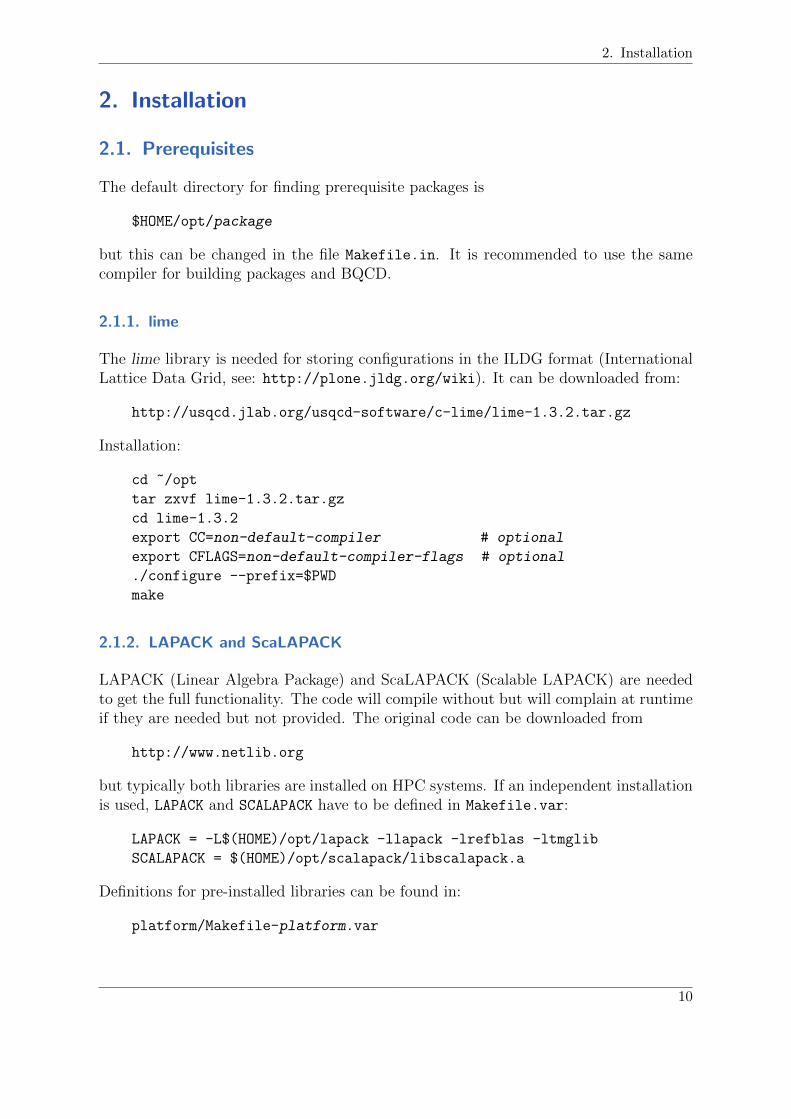
2.1. Prerequisites
The default directory for finding prerequisite packages is
$HOME/opt/package
but this can be changed in the file Makefile.in. It is recommended to use the samecompiler for building packages and BQCD.
2.1.1. lime
The lime library is needed for storing configurations in the ILDG format (InternationalLattice Data Grid, see: http://plone.jldg.org/wiki). It can be downloaded from:
http://usqcd.jlab.org/usqcd-software/c-lime/lime-1.3.2.tar.gz
Installation:
cd ~/opt
tar zxvf lime-1.3.2.tar.gz
cd lime-1.3.2
export CC=non-default-compiler # optional
export CFLAGS=non-default-compiler-flags # optional
./configure --prefix=$PWD
make
2.1.2. LAPACK and ScaLAPACK
LAPACK (Linear Algebra Package) and ScaLAPACK (Scalable LAPACK) are neededto get the full functionality. The code will compile without but will complain at runtimeif they are needed but not provided. The original code can be downloaded from
http://www.netlib.org
but typically both libraries are installed on HPC systems. If an independent installationis used, LAPACK and SCALAPACK have to be defined in Makefile.var:
LAPACK = -L$(HOME)/opt/lapack -llapack -lrefblas -ltmglib
SCALAPACK = $(HOME)/opt/scalapack/libscalapack.a
Definitions for pre-installed libraries can be found in:
platform/Makefile-platform.var
10

2. Installation
2.2. Download
The source code of BQCD and this manual can be downloaded from:
https://www.rrz.uni-hamburg.de/bqcd
2.3. License
BQCD is free software: you can redistribute it and/or modify it under the terms ofthe GNU General Public License as published by the Free Software Foundation, eitherversion 3 of the License, or (at your option) any later version.
BQCD is distributed in the hope that it will be useful, but WITHOUT ANY WAR-RANTY; without even the implied warranty of MERCHANTABILITY or FITNESSFOR A PARTICULAR PURPOSE. See the GNU General Public License for more de-tails.
You should have received a copy of the GNU General Public License along with BQCD.If not, see <http://www.gnu.org/licenses/>.
2.4. Configuration
2.4.1. Supported platforms
Platform dependent parts are kept in Makefile.var which is a symbolic link to a file inthe platform directory
Makefile.var -> platform/Makefile-platform.var
for example:
Makefile.var -> platform/Makefile-gnu.var
One can prepare working on a particular platform by entering the command
make prep-platform
which creates the symbolic link, for example:
make prep-gnu
In the platform directory one can find files for machines that were used in the past butthat are not necessarily up-to-date. Currently you can expect that compilation worksin these cases:
11

2. Installation
gnu GNU compiler, Open-MPI/MPICHhlrn3 Cray XC40 (Intel compiler, Cray MPI)intel Intel compiler, Intel MPIjuqueen IBM BlueGene/Q at JSC Julich
2.4.2. Settings in Makefile.var
In Makefile.var one can make the following high level settings:
timing = empty or 1 switch on profilingmpi = empty or 1 single processor program or MPIomp = empty or 1 compile with OpenMPdebug = empty or 1 compile with debug flagslibd = 100 which hopping matrix multiplicationrandom = ranlux-3.2 which random number generator
Based on these high level settings, several low level settings are made. This includescompiler flags, preprocessor flags and which libraries are used. For more information,see platform/Makefile-EXPLAINED.var.
The make procedure is not always straightforward. Instead of make,
make fast
just builds the binary bqcd5.
2.4.3. Configuring/porting SIMD
Configuring/porting SIMD is described in cg/README.
2.5. Testing
Reference test runs can be found in the data/ directory. For each case there is an inputand reference output file:
bqcd.NNN.input
bqcd.NNN.output
The test cases are described in comments:
grep comment *.input
A test run looks like this:
12

2. Installation
cd data
../bqcd5 bqcd.NNN.input bqcd.NNN.res
diff bqcd.NNN.output bqcd.NNN.res
Due to rounding differences the output will not be identical to the reference output butshould be very close to the reference output.
In order to test a parallel run
• set the number of processes to be used for each lattice dimension in the input file,for example
processes 1 1 2 4
decomposes the z- into 2 domains and the t-direction into 4 domains,
• run BQCD on the appropriate number on processes (8 in the above example):
mpirun -np 8 ../bqcd5 bqcd.NNN.output bqcd.NNN.res
In principle the output (bqcd.NNN.res) is identical to the output from the sequen-tial run (again up to rounding differences). This holds true for any decomposition.
13
3. Usage
3. Usage
3.1. Quickstart guide
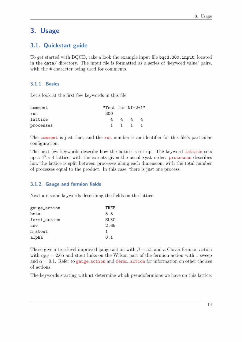
To get started with BQCD, take a look the example input file bqcd.300.input, locatedin the data/ directory. The input file is formatted as a series of ‘keyword value’ pairs,with the # character being used for comments.
3.1.1. Basics
Let’s look at the first few keywords in this file:
comment "Test for Nf=2+1"
run 300
lattice 4 4 4 4
processes 1 1 1 1
The comment is just that, and the run number is an identifier for this file’s particularconfiguration.
The next few keywords describe how the lattice is set up. The keyword lattice setsup a 43 × 4 lattice, with the extents given the usual xyzt order. processes describeshow the lattice is split between processes along each dimension, with the total numberof processes equal to the product. In this case, there is just one process.
3.1.2. Gauge and fermion fields
Next are some keywords describing the fields on the lattice:
gauge_action TREE
beta 5.5
fermi_action SLRC
csw 2.65
n_stout 1
alpha 0.1
These give a tree-level improved gauge action with β = 5.5 and a Clover fermion actionwith cSW = 2.65 and stout links on the Wilson part of the fermion action with 1 sweepand α = 0.1. Refer to gauge action and fermi action for information on other choicesof actions.
The keywords starting with nf determine which pseudofermions we have on this lattice:
14

3. Usage
nf2_kappa1 0.121095
nf2_kappa1h1 0.1203
hmc_hkappa 1
nf1_kappa1 0.120512
nf1_kappa1npf 2
nf1_kappa1nth 4
This is a Nf=2+1 run with two kinds of pseudofermions:
• nf2 kappa1 produces a double-flavour pseudofermion with hopping parameter κ =0.121095, which has a Hasenbusch filter given by nf2 kappa1h1 at κ′ = 0.1203.hmc hkappa toggles which form of Hasenbusch is used (κ′ or κ+ ρ).
• nf1 kappa1 produces a single-flavour pseudofermion with κ = 0.120512 via RHMC,which is constructed via two pseudofermions (nf1 kappa1npf) with a rational ap-proximation R(M †M) ≈ (M †M)−1/4 (nf1 kappa1nth).
3.1.3. Molecular dynamics
Now for some information about how the molecular dynamics part of HMC is integrated:
hmc_trajectory_length 1.0
hmc_integrator1 2MNSTS
hmc_integrator2 2MNSTS
hmc_integrator3 2MNSTS
hmc_integrator4 2MNSTS
hmc_steps 5
hmc_m_scale 2
hmc_m_scale2 2
hmc_m_scale3 2
hmc_dsf_k11 2
hmc_dsf_k12 3
hmc_dsfr_k1 1
hmc_dsd 2
hmc_dsig 3
hmc_dsg 4
The trajectory length is τ = 1, with a total of 4 different integration time-scales withthe second order minimal norm integrator 2MNSTS on each scale; see hmc integrator
for other options. There are 5 integration steps on scale number 1 hmc steps, two stepsnested within this for scale number 2 hmc m scale, then nested with two steps again for
15

3. Usage
scales 3 then 4. Instead of nested integrators, one can use generalized integrators whereeach time-scale’s integration scheme is independent: see section 5.4 for more information.
The time-scale numberings are referenced by the time scale specifiers which follow. Thesetup of this file leads to the following distribution of action terms on each time scale:
1. The single-fermion pseudofermion term (hmc dsfr k1)
2. The heavier Hasenbusch term (hmc dsf k11) and the Clover determinant (hmc dsd)
3. The Hasenbusch correction term (hmc dsf k12) and the improved part of the gluonaction (hmc dsig)
4. The plaquette/Wilson part of the gluon action (hmc dsg)
3.1.4. Markov Chain
Next are some parameters setting up the Markov chain
hmc_accept_first 10
start_configuration hot
start_random 319503
mc_steps 10
mc_total_steps 20000
mc_save_frequency 0
This causes a hot start for the gauge field (start configuration) with random seed’319503’ (start random). 10 trajectories are calculated during each run of the code(mc steps) with the first 10 undergoing forced acceptance (hmc accept first). Noconfigurations are saved to file (mc save frequency), and the code stops after 20,000trajectories (mc total steps). The default for mc_total_steps is low, and shouldusually be set.
3.1.5. Fermion matrix inversion
Solver parameters:
solver_rest 1e-11
solver_rest_md 1e-9
solver_rest_cg_ritz 1e-11
solver_maxiter 1200
...
solver_outer_solver cg
...
16
3. Usage
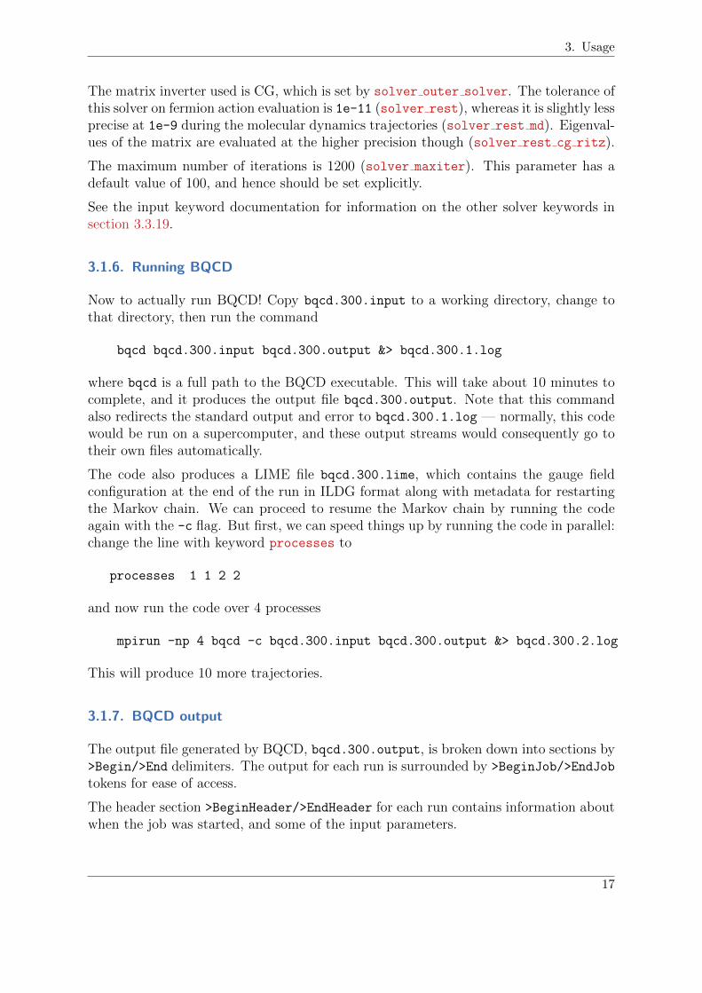
The matrix inverter used is CG, which is set by solver outer solver. The tolerance ofthis solver on fermion action evaluation is 1e-11 (solver rest), whereas it is slightly lessprecise at 1e-9 during the molecular dynamics trajectories (solver rest md). Eigenval-ues of the matrix are evaluated at the higher precision though (solver rest cg ritz).
The maximum number of iterations is 1200 (solver maxiter). This parameter has adefault value of 100, and hence should be set explicitly.
See the input keyword documentation for information on the other solver keywords insection 3.3.19.
3.1.6. Running BQCD
Now to actually run BQCD! Copy bqcd.300.input to a working directory, change tothat directory, then run the command
bqcd bqcd.300.input bqcd.300.output &> bqcd.300.1.log
where bqcd is a full path to the BQCD executable. This will take about 10 minutes tocomplete, and it produces the output file bqcd.300.output. Note that this commandalso redirects the standard output and error to bqcd.300.1.log — normally, this codewould be run on a supercomputer, and these output streams would consequently go totheir own files automatically.
The code also produces a LIME file bqcd.300.lime, which contains the gauge fieldconfiguration at the end of the run in ILDG format along with metadata for restartingthe Markov chain. We can proceed to resume the Markov chain by running the codeagain with the -c flag. But first, we can speed things up by running the code in parallel:change the line with keyword processes to
processes 1 1 2 2
and now run the code over 4 processes
mpirun -np 4 bqcd -c bqcd.300.input bqcd.300.output &> bqcd.300.2.log
This will produce 10 more trajectories.
3.1.7. BQCD output
The output file generated by BQCD, bqcd.300.output, is broken down into sections by>Begin/>End delimiters. The output for each run is surrounded by >BeginJob/>EndJob
tokens for ease of access.
The header section >BeginHeader/>EndHeader for each run contains information aboutwhen the job was started, and some of the input parameters.
17

3. Usage
The main part of the output file contains a series of embedded tables. These tablescontain special tokens of the form T%XX and %XX such that we can use grep to extractthem.
We can extract general information about the Markov Chain progress by running
grep ’%mc’ bqcd.300.output
This will give information about the plaquette, acceptance rate and iterations counts foreach trajectory:
T%mc traj e f PlaqEnergy exp(-Delta_H) Acc CGcalls CGitTot CGitMax CGMcalls CGMitTot CGMitMax Plaquette
%mc 1 1 1 0.4603695377 0.9406814248 1 53 2422 61 0 0 0 0.539630462296880
%mc 2 1 1 0.4597443535 0.9182754364 1 53 2290 55 0 0 0 0.540255646459386
%mc 3 1 1 0.4608069194 1.0295291357 1 53 2308 57 0 0 0 0.539193080649400
%mc 4 1 1 0.4591734179 1.0057202626 1 53 2206 55 0 0 0 0.540826582090360
%mc 5 1 1 0.4744552445 0.9244531373 1 53 1985 51 0 0 0 0.525544755494560
%mc 6 1 1 0.4717006653 0.9892924489 1 53 2011 47 0 0 0 0.528299334696576
%mc 7 1 1 0.4612058658 0.9370571005 1 53 2039 52 0 0 0 0.538794134178326
%mc 8 1 1 0.4527961003 0.9920165839 1 53 1989 50 0 0 0 0.547203899705222
%mc 9 1 1 0.4516703478 0.9742350535 1 53 2064 49 0 0 0 0.548329652150200
%mc 10 1 1 0.4544061729 0.9963916062 1 53 2105 51 0 0 0 0.545593827098611
T%mc traj e f PlaqEnergy exp(-Delta_H) Acc CGcalls CGitTot CGitMax CGMcalls CGMitTot CGMitMax Plaquette
%mc 11 1 1 0.4609078806 1.0152287442 1 53 2067 52 0 0 0 0.539092119360002
%mc 12 1 1 0.4563820740 0.9691243600 1 53 2114 49 0 0 0 0.543617925997414
%mc 13 1 1 0.4684701708 0.9935836158 1 53 2039 53 0 0 0 0.531529829236492
%mc 14 1 1 0.4651568757 1.0140884160 1 53 2019 49 0 0 0 0.534843124331008
%mc 15 1 1 0.4502802111 0.9663791611 1 53 2021 50 0 0 0 0.549719788863034
%mc 16 1 1 0.4505187147 1.0078377885 1 53 1995 49 0 0 0 0.549481285258094
%mc 17 1 1 0.4468129429 0.9965722228 1 53 2023 50 0 0 0 0.553187057109728
%mc 18 1 1 0.4473054753 0.9839808214 1 53 2033 50 0 0 0 0.552694524687057
%mc 19 1 1 0.4452533591 1.0368457399 1 53 2116 50 0 0 0 0.554746640879882
%mc 20 1 1 0.4518358652 0.9818649052 1 53 2175 54 0 0 0 0.548164134753665
%mc 21 1 1 0.4637735116 0.9187633143 1 53 2126 53 0 0 0 0.536226488442716
%mc 22 1 1 0.4719595030 0.9990389368 1 53 2123 50 0 0 0 0.528040497005646
%mc 23 1 1 0.4711059887 1.0049051498 1 53 2262 53 0 0 0 0.528894011297565
%mc 24 1 1 0.4630871801 0.9687888230 1 53 2176 53 0 0 0 0.536912819873419
%mc 25 1 1 0.4773637154 0.9786564332 1 53 2228 52 0 0 0 0.522636284633002
%mc 26 1 1 0.4818968039 0.9527153539 1 53 2321 56 0 0 0 0.518103196065121
%mc 27 1 1 0.4849282090 0.9596876019 1 53 2287 57 0 0 0 0.515071791018083
%mc 28 1 1 0.4736714060 1.0016959817 1 53 2210 54 0 0 0 0.526328593955653
%mc 29 1 1 0.4736714060 0.9708984380 0 53 2235 54 0 0 0 0.526328593955653
%mc 30 1 1 0.4662033473 0.9745797939 1 53 2074 52 0 0 0 0.533796652740701
For the first 10 trajectories which were force-accepted, this data is contained in the tablemarked %fa instead.
We can also look at an iteration count breakdown in the table %it, and the average%Favg and maximal %Fmax forces. A comprehensive list of the embedded tables can befound in section 3.7.7.
A footer section >BeginFooter/>EndFooter for each run has the completion time of thejob and the total CPU-Time.
At the end of each run is a timing section >BeginTiming/>EndTiming, which containsruntime statistics on many different operations within the code.
18

3. Usage
3.2. Command line
BQCD takes the following arguments:
bqcd [-c] input [output]
bqcd --convert-to-ildg input [output]
bqcd -I
bqcd -V
3.2.1. Flag -c (continuation job)
If the -c parameter is present the start configuration is being read from file. Otherwisea start configuration is being generated. The setup is such that input does not have tobe modified from the first to the second job in a job chain.
3.2.2. Flag --convert-to-ildg
This flag is used to convert saved configuration from BQCD formats to the ILDG format(see section 6.7). Example:
• work with bqcd.200.input and modify io conf format (i.e. switch from ildg tobqcd2 format)
io_conf_format "bqcd2"
• run BQCD
bqcd bqcd.200.input bqcd.200.output &> bqcd.200.3.log
• convert the gauge field configuration of trajectory 10 to ILDG format
bqcd --convert-to-ildg bqcd.200.00010.info bqcd.200.00010.output
3.2.3. Flag -I (print default input values)
If -I is given the program prints all possible input parameters with their default valuesand exits. Most of them are described in section 3.3.
3.2.4. Flag -V (print program version)
The program prints version information and exits. The output looks like this:
This is bqcd 5.1 (revision 887)
input format: 5
conf info format: 4
19

3. Usage
MAX_TEMPER: 50
REAL kind: 8
Version of D: 100
Communication: MPI (sc:immediate) (g:immediate) + OpenMP
RandomNumbers: ranlux-3.2 level 2
3.2.5. Argument input
Name of input parameter file.
3.2.6. Argument output
Name of log- and results file. If not given data will be written to stdout. If the file doesnot exist it will be created. If -c is set new output will be appended to the file. If -c isnot set an existing file will be overwritten.
3.3. Input parameters and the syntax of input file
The syntax of the input file is one keyword value(s) pair (or tuple) per line. Emptylines and lines beginning with a # character are ignored. Keywords are checked forvalidity but the number of values and the types of values are not. It is a good idea toenclose character string parameters in double quotes "..." (in particular Fortran mightscramble filenames containing slashes).
The following input keyword documentation is fairly self-explanatory but some keywordtypes are worth noting. An enum is a string which takes certain built-in values anda flag is an integer which switches a feature on and off, usually with off = 0 and onotherwise.
3.3.1. General parameters
run
Type: integer; Default: 0
An integer that specifies the run number of the job. This is stored in gener-ated configurations, such that restarts are performed correctly. Try to giveeach distinct input file a different run number.
comment
Type: string; Default: ""
A comment, which is (only) added to the header of the output. Useful toidentify what configuration of parameters you are using.
20
3. Usage
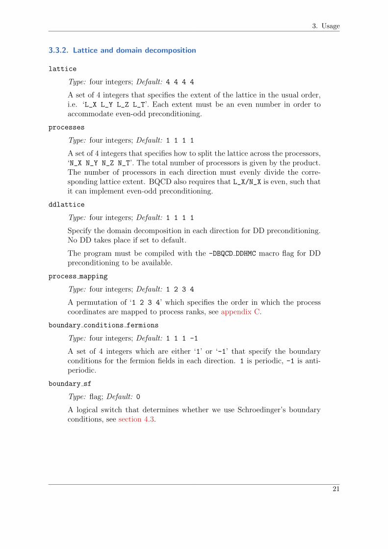
3.3.2. Lattice and domain decomposition
lattice
Type: four integers; Default: 4 4 4 4
A set of 4 integers that specifies the extent of the lattice in the usual order,i.e. ‘L_X L_Y L_Z L_T’. Each extent must be an even number in order toaccommodate even-odd preconditioning.
processes
Type: four integers; Default: 1 1 1 1
A set of 4 integers that specifies how to split the lattice across the processors,‘N_X N_Y N_Z N_T’. The total number of processors is given by the product.The number of processors in each direction must evenly divide the corre-sponding lattice extent. BQCD also requires that L_X/N_X is even, such thatit can implement even-odd preconditioning.
ddlattice
Type: four integers; Default: 1 1 1 1
Specify the domain decomposition in each direction for DD preconditioning.No DD takes place if set to default.
The program must be compiled with the -DBQCD DDHMC macro flag for DDpreconditioning to be available.
process mapping
Type: four integers; Default: 1 2 3 4
A permutation of ‘1 2 3 4’ which specifies the order in which the processcoordinates are mapped to process ranks, see appendix C.
boundary conditions fermions
Type: four integers; Default: 1 1 1 -1
A set of 4 integers which are either ‘1’ or ‘-1’ that specify the boundaryconditions for the fermion fields in each direction. 1 is periodic, -1 is anti-periodic.
boundary sf
Type: flag; Default: 0
A logical switch that determines whether we use Schroedinger’s boundaryconditions, see section 4.3.
21

3. Usage
3.3.3. Gauge action
Refer to section 4.1 for further explanation of gauge actions.
gauge action
Type: enum; Default: WILSON
A string that specifies which gauge action to use.
• WILSON: use the Wilson gauge action
• TREE: use the tree-level improved action
• IWASAKI: use the Iwasaki action
See section 4.1 for expressions of these actions.
beta
Type: float; Default: 0.0
Defines β, the inverse coupling of the SU(3) gauge.
hmc dsg
Type: integer; Default: 0
Specifies the time-scale on which the plaquette (Wilson) gluon action Splaq
is integrated.
hmc dsig
Type: integer; Default: 0
Specifies the time-scale on which the improved part of the gluon action Simp =Sg − Splaq is integrated.
3.3.4. Fermion action
Refer to section 4.2 for further information on fermion actions. For κ values, seenf2 kappa[1-6] and nf1 kappa[1-6].
fermi action
Type: enum; Default: NON
A string that specifies which fermion action to use.
• NON: no fermions; just do gluodynamics
• WILSON: use the Wilson fermion action
• CLOVER: use the O(a)-improved ’clover’ fermion actionRequires csw
• SLW: use the Wilson fermion action with stout links
22
3. Usage
Requires alpha, n stout
• SLIC: same as CLOVER, but with stout links in the clover termRequires csw, alpha, n stout
• SLRC: same as CLOVER, but with stout links in the Wilson termRequires csw, alpha, n stout
• SLOC: same as CLOVER, but with stout links in both termsRequires csw, alpha, n stout
See section 4.2 for expressions of these actions.
h
Type: float; Default: 0.0
Defines h, the twisted mass parameter for explicit parity-flavour symmetrybreaking. See section 4.2 for the corresponding action term.
chemi
Type: float; Default: 0.0
Defines the real part of the chemical potential µ. See section 4.2 for anexplanation.
chemi i
Type: float; Default: 0.0
Defines the imaginary part of the chemical potential µ. See section 4.2 foran explanation.
breaking term
Type: file; Default: ""
Specifies the path to the matrix formed file to violate CPT symmetries withλ (nf2 lambda[1-6] and nf1 lambda[1-6]), see section 4.2.
n stout
Type: integer; Default: 0
Required for : a stout-link fermion action
Determines how many times to smear the gauge links for a stout link fermionaction. See section 4.2 for an explanation.
alpha
Type: float; Default: 0.0
Required for : a stout-link fermion action
Sets the parameter α for stout link smearing. See section 4.2 for an expla-nation.
23

3. Usage
csw
Type: float; Default: 0.0
Required for : a clover fermion action
Defines cSW , the Symanzik improvement coefficient for clover actions.
hmc dsd
Type: integer; Default: 0
Required for : a clover fermion action
Specifies the time-scale on which the clover determinant is integrated.
3.3.5. Double-flavour pseudofermions
nf2 kappa[1-6]
Type: float; Default: 0.0
Specifies κ for up to 6 distinct double-flavour pseudofermions.
nf2 kappa[1-6]h[1-3]
Type: float; Default: 0.0
Specifies up to three Hasenbusch masses for each double-flavour pseudofermion.These are ordered finest to coarsest, which is reverse to the usual action or-dering: e.g. nf2_kappa1h1 is heavier than nf2_kappa1h2. See the section 5.1for more information.
hmc hkappa
Type: flag; Default: 0
Toggles the way Hasenbusch masses are implemented from the given valuesnf2 kappa[1-6]h[1-3].
• On (non-zero): given values are modified κ parameters κ′, such thatW = K(κ′)
• Off: given values are ρ shifts, such that W = K(κ) + ρ.
nf2 lambda[1-6]
Type: float; Default: 0.0
Specifies λ for up to 6 distinct double-flavour pseudofermions to violate CPTsymmetries with breaking term, see section 4.2.
hmc dsf k[1-6][1-4]
Type: integer; Default: 0
Specifies the time-scale on which the jth mass-preconditioned term for the
24

3. Usage
ith two-flavour fermion is integrated.
The ordering of the action terms is the reverse of the action term ordering;see section 3.3.18 for more information.
3.3.6. Single-flavour pseudofermions
nf1 kappa[1-6]
Type: float; Default: 0.0
Specifies κ for up to 6 distinct single-flavour fermions.
nf1 kappa[1-6]npf
Type: integer; Default: 1
Specifies how many degenerate pseudo-fermions there are for each specifiedsingle-flavour fermion.
nf1 kappa[1-6]nth
Type: integer; Default: 2
Specifies the n-th root of K = M †M to be approximated by the RHMCrational approximation for each single-flavour fermion.
nf1 lambda[1-6]
Type: float; Default: 0.0
Specifies λ for up to 6 distinct single-flavour pseudofermions to violate CPTsymmetries with breaking term, see section 4.2.
hmc dsfr k[1-6]
Type: integer; Default: 0
Specifies the time-scale on which the RHMC term is integrated for eachsingle-flavour fermion. See time-scale section section 3.3.18 for more infor-mation.
rescale rhmc
Type: flag; Default: 1
Determines (non-zero = on) whether to rescale the RHMC approximationafter each trajectory. If the ratapp has range [lmin, lmax] and the fermionmatrix has eigenvalue range [λmin, λmax], we can use
R(K) ≈ Kn = a−n(aK)n ≈ a−nR(aK) (1)
to centre the approximation’s effective range on the true eigenvalue spectrum.
25

3. Usage
Namely, R(aK) is effective on [lmin/a, lmax/a], so we choose a such that
lmaxaλmax
=aλminlmin
=⇒ a =
√lminlmaxλminλmax
Turning this off is useful when comparing methods, as it ensures that therational approximation does not change.
3.3.7. RHMC tuning parameters
tuning approx range
Type: flag; Default: 0
Turns on tuning of rational approximation.
tuning approx range list
Type: file; Default: ""
Specifies file to tuning rational approximation, see data/rangelist in thesource code for an example.
tuning fraction tolerance
Type: file; Default: ""
Specifies file to tuning fraction tolerances, see data/fractiontolerance in thesource code for an example.
3.3.8. Zolotarev rational approximation
For an brief explanation of the Zolotarev approximation, see section 5.6.
hmc zolo
Type: flag; Default: 0
A switch that determines whether the program uses a Zolotarev rational ap-proximation for RHMC rather than the built-in Remez algorithm for the casewhere nf1 kappa[1-6]nth=2. It only takes effect for such pseudofermionsbecause the Zolotarev rational approximation is an approximation to theinverse square root.
hmc zolo n
Type: integer; Default: 0
Specifies the number of shifts n to use in the Zolotarev approximation.If omitted, the number of shifts is calculated to produce the error delta
26
3. Usage
hmc zolo delta on the given approximation range hmc zolo [min|max].
hmc zolo delta
Type: float; Default: 1e-6
Specifies the error delta for the Zolotarev approximation, which is the max-imum error of the approximation over the eigenvalue range specified byhmc zolo [min|max].
If both hmc zolo delta and hmc zolo n are given, the latter takes prefer-ence, and the code will issue a warning if the produced rational approxima-tion has a larger error delta.
hmc zolo [min|max]
Type: integer; Default: 0
Specifies the minimum/maximum eigenvalue bound to approximate in theZolotarev approximation. If omitted, the eigenvalue range is taken to be[0.8λmin, 1.2λmax], where λmin/λmax is the calculated minimum/maximumeigenvalue for the fermion matrix M †M .
3.3.9. QED
For more information on using QED, see section 4.4.
beta qed
Type: float; Default: 0.0
Defines βQED, the inverse coupling of the electromagnetic force.
nf2 em charge[1-6] x3
Type: integer; Default: 0
Defines how many thirds of the electron charge the ith double-flavour pseud-ofermion has.
nf1 em charge[1-6] x3
Type: integer; Default: 0
Defines how many thirds of the electron charge the ith single-flavour pseud-ofermion has.
3.3.10. Axion
kappa axion
Type: float; Default: 0.0
27

3. Usage
Defines κa, the hopping parameter of axion. See section 4.5.
finv axion
Type: float; Default: 0.0
Defines finv, a relevant parameter of the inverse decay constant of axion. Seesection 4.5.
3.3.11. PFHMC
For an explanation of polynomial filtering, including the formulation of the polynomialsused, see section 5.3.
nf2 k[1-6]p[1-3]
Type: integer; Default: 0
Specifies up to 3 polynomial filters via their order for each possible two-flavour degenerate pseudo-fermion. They are expected to be ordered fromfinest to coarsest, meaning that (for example) nf2_k1p1 > nf2_k1p2. Thegiven polynomial orders are passed to the Chebyshev polynomial creationroutines to create polynomials of suitable order and (µ, ν).
nf2 k[1-6] [mu|nu]
Type: float; Default: 0.0
Specifies the value of the µ/ν parameter for the Chebyshev polynomial usedin PFHMC for each double-flavour pseudofermion. Together, these two pa-rameters specify the ellipse upon which the roots of the Chebyshev polyno-mials lay: see section 5.3 for further explanation.
nf2 k[1-6]p[1-3] file
Type: file; Default: ""
Specifies up to three polynomial filters for each possible double-flavour pseudo-fermion which are loaded from the specified file. This file should contain thefollowing
• Line 1: the polynomial order n
• Lines 2 to n+ 1: the polynomial roots zi, specified as complex numbersvia 2-tuples (x,y) = x+ iy.
IMPORTANT: the current implementation of polynomial filtering as-sumes that z∗i = zn−i+1, so the roots should be specified in an orderthat obeys this.
See data/testpoly nf2 p4.txt for an example.
The polynomials are expected to be defined from finest to coarsest, i.e. in
28
3. Usage
decreasing order.
The polynomial is loaded directly into the action term, giving Si = φ†iP (K)φi.This is important to note when using multiple filters. The polynomial forthe correction term φ†[KP (K)]−1φ is calculated in the code as the productof all the polynomial filters P (K) plus a zero root K.
hmc dsfp k[1-6][1-4]
Type: integer; Default: 0
Specifies the integration time-scales for each part of the specified polynomial-filtered actions.
Note that due to the way the polynomial filters are initialized, the actionterms are in the reverse order. See section 3.3.18 for more details.
nf1 k[1-6]p1
Type: integer; Default: 0
Specifies a polynomial filter via its order for each single-flavour pseudo-fermion. This polynomial is a built-in Chebyshev polynomial that approxi-mates the inverse square root over the range [5e-3,3].
For more polynomial filters in PF-RHMC, please use the polynomial readingfacilities provided by nf1 k1p1 file.
nf1 k[1-6]p[1-3] file
Type: file; Default: ""
Specifies up to three polynomial filters for each possible single-flavour pseudo-fermion via loading from the specified file. They are expected to be definedfrom finest to coarsest.
See nf1 k[1-6]p[1-3] file for an explanation of the file format. An exam-ple file is available at data/testpoly nf1 p4.txt.
The polynomial for the correction term φ†P (K)−1R(K)φ is calculated in thecode as the product of all the polynomial filters.
hmc dsfr k[1-6]p[1-3]
Type: integer; Default: 0
Specifies the integration time-scales for each part of the specified polynomial-filtered actions for single-flavour pseudo-fermions.
Note that due to the way the polynomial filters are initialized, the actionterms are in the reverse order. See section 3.3.18 for more details.
29
3. Usage
3.3.12. Truncated rational HMC (tRHMC)
For an explanation of truncated RHMC, see section 5.5. Note that the current imple-mentation requires the use of the Zolotarev approximation (hmc zolo).
nf1 k[1-6] trunc[1-3]
Type: integer; Default: 0
Specifies up to 3 truncation indices for each single-flavour rational approx-imation RHMC. The specified indices are the points at which the rationalapproximation is cut, with the ratapp shifts being ordered from largest t=1
to smallest t=n.
As the code assumes filters are ordered from finest to coarsest, the filtersshould be decreasing.
hmc dsfr k[1-6]t[1-3]
Type: integer; Default: 0
Specifies the integration time-scales for tRHMC actions. These are orderedin reverse relative to the action terms, see section 3.3.18 for more details.
3.3.13. Start parameters
The following parameters only take effect if the -c flag is not used, implying that thejob is an initial HMC run.
start configuration
Type: enum; Default: cold
A string that determines how the initial gauge configuration is produced:
• cold: start from scratch with U = I
• hot: start from scratch with U set randomly
• file: load from a given file. Requires start ildg file xor start info file.
start ildg file
Type: file; Default: ""
Specifies the ILDG .lime file from which we should read the initial gaugeconfiguration. Mutually exclusive with start info file.
start info file
Type: file; Default: ""
Specifies the BQCD .info file from which we should read the initial gaugeconfiguration. Mutually exclusive with start ildg file.
30
3. Usage
start random
Type: enum or integer; Default: ""
Specifies the random seed (an integer) that initializes the random numbergenerator at the start of a Markov chain:
• default: use a default seed built into BQCD.
• random: produce a seed at random.
• (integer): use the given integer as the seed.
Of these three options, the third is recommended as this ensures that theruns are reproducible yet still ‘random’ between different runs.
3.3.14. Configuration I/O
For further information, see section 3.4 to section 3.6.
io restart format
Type: enum; Default: bqcd
Specify the format [bqcd|bqcd2|ildg] for reading/saving configurations atthe start/end of each execution for checkpointing. Such configurations aresaved at the end of every execution of the code, and read when starting acontinuation run via -c (see also section 6.7).
io conf format
Type: enum; Default: bqcd
Specify the format [bqcd|bqcd2|ildg] for saving configurations after cer-tain trajectories as specified by mc save frequency (see also section 6.7).
io bqcd restart filename
Type: string; Default: "bqcd.%R3"
Specify the names (w/o extension) of checkpoint/restart files in bqcd orbqcd2 io restart format (for the %-macro expansion see section 3.5).
io bqcd conf filename
Type: string; Default: "bqcd.%R3.%T5"
Specify the names (w/o extension) of files for saved configurations in bqcd
or bqcd2 io conf format (for the %-macro expansion see section 3.5).
ildg precision
Type: integer; Default: 64
Sets the precision (in bits [32|64]) for ILDG files saved explicitly viamc save frequency.
31

3. Usage
ildg precision restart
Type: integer; Default: 64
Sets the precision (in bits [32|64]) for checkpoint ILDG files.
ildg filename prefix
Type: string; Default: "bqcd.%R3"
Specifies the prefix used when explicitly outputting ILDG files. This shouldcontain information about the simulated ensemble as a whole. (for the %-macro expansion see section 3.5)
Saved ILDG configurations are named <prefix><middle>.<extension>, andILDG restart files are named bqcd.<run>.<extension>, where
• <prefix> = ildg filename prefix
• <middle> = ildg filename middle
• <extension> = ildg filename extension
• <run> = run
ildg filename middle
Type: string; Default: ".%T5"
Specifies the ‘middle’ part used when explicitly outputting ILDG files. Thisshould about contain information each individual configuration. (for the%-macro expansion see section 3.5)
ildg filename extension
Type: string; Default: "lime"
Specifies the extension part used when outputting ILDG files.
ildg template ensemble
Type: file; Default: ""
Specifies the path to the template XML file for saving ensemble metadata.The produced ensemble XML file is saved as <prefix>.xml
(see ildg filename prefix for an explanation).
ildg template conf
Type: file; Default: ""
Specifies the path to the template XML file for saving per-configuration meta-data. The produced configuration XML files are saved as <prefix><middle>.xml(see ildg filename prefix for an explanation).
ildg markov chain uri
Type: string; Default: "mc://UNDEFINED"
32
3. Usage
Specifies the Markov Chain URI to be placed in the ensemble XML file.It fills out the corresponding template parameter in the XML file. Thisinformation is used for tagging on an ILDG database.
ildg data lfn path
Type: string; Default: "lfn://UNDEFINED"
Specifies the LFN for the ensemble XML file. It fills out the correspondingtemplate parameter in the XML file. This information is used for tagging onan ILDG database.
ildg participant name
Type: string; Default: ""
Field for the code user’s name in the XML files. It fills out the correspondingtemplate parameter in the XML file.
ildg participant institution
Type: string; Default: ""
Field for the code user’s institution in the XML files. It fills out the corre-sponding template parameter in the XML file.
ildg machine name
Type: string; Default: ""
Field for the name of the machine BQCD is used on in the XML files. It fillsout the corresponding template parameter in the XML file.
ildg machine institution
Type: string; Default: ""
Field for the institution of the machine BQCD is used on in the XML files.It fills out the corresponding template parameter in the XML file.
ildg machine type
Type: string; Default: ""
Field for the type of the machine BQCD is used on (e.g. BlueGene) in theXML files. It fills out the corresponding template parameter in the XMLfile.
3.3.15. Markov Chain
mc steps
Type: integer; Default: 1
An integer that specifies how many Markov Chain trajectories should be
33

3. Usage
calculated for this execution run.
mc save frequency
Type: integer; Default: 1
An integer that specifies how often to save the gauge configuration. Ifmc save frequency = n, then every nth gauge field configuration is saved tofile. The file type is specified by io conf format.
mc total steps
Type: integer; Default: 1
An integer that specifies the maximum number of Markov Chain trajectoriesthat should be calculated over all runs from this input file. When the tra-jectory counter reaches this number, a .STOP file is produced and no moretrajectories are calculated.
3.3.16. Hybrid Monte Carlo
hmc trajectory length
Type: integer; Default: 1
Specifies the length τ of each trajectory.
hmc accept first
Type: integer; Default: 0
An integer that specifies how many trajectories at the start of a simulationare forced to be accepted. This is necessary for some configurations to ensurewe don’t get stuck. The force acceptance can span several runs of the code.The logs for these trajectories are given in the table %fa.
This should be set to zero if starting from a file, as forced acceptance willinevitably take the system out of equilibrium.
hmc test
Type: flag; Default: 0
An integer that acts as a logical flag for HMC reversibility testing. Thiscauses BQCD to calculate a trajectory both forwards and backwards, reporton the difference between the initial and final states in the section HMCtest
of the output file, then finish.
3.3.17. Integrator specification
hmc steps
34
3. Usage
Type: integer; Default: 0
An integer that specifies how many integration steps to take per trajectoryat the coarsest scale, time-scale #1. The corresponding step-size h is givenby h = τ
nsteps.
hmc genint
Type: flag; Default: 0
A flag for activating the use of the generalized multi-scale integration scheme,as opposed to the default nested multi-scale scheme. This scheme overlaysdifferent integration schemes for each time-scale onto a single time step axis,such that any number of steps can be used on each time-scale. See section 5.4for more details.
Note that using the generalized scheme changes the meaning of hmc m scale.
hmc m scale, hmc m scale[2-5]
Type: integer; Default: 1
An integer that specifies, by default, the relative scaling between successivetime-scales. If hmc genint is on, then this keyword specifies the absolutenumber of integration steps at this time-scale.
In the default case, if hmc_m_scale=2, then for every space update step atthe top level we have two integration steps at the second level. Note thatthis does not necessarily mean there are 2 space steps on the second level forevery space step in the top level – an integration step can have several spacesteps.
The time scales are indexed as 1:hmc_steps, 2:hmc_m_scale, 3:hmc_m_scale2etc. This indexing is used by both the time-scale specification keywords (sec-tion 3.3.18), and the integrator specification keywords hmc integrator.
hmc integrator[1-6]
Type: enum; Default: LPFSTS for 1–3, NON for 4–6
Strings that specify which integrators to use at each time-scale. and must bespecified for each time-scale used. The number of integration steps at eachtime-scale are defined via hmc steps and hmc m scale.
• LPFSTS: use the space-time-space leapfrog integrator
• LPFTST: use the time-space-time leapfrog integrator
• 2MNSTS: use the space-time-space 2nd order minimal-norm integrator
• 2MNTST: use the time-space-time 2nd order minimal-norm integrator
• 4MN4FP: use the position-space version of the 4th order minimal-normintegrator
35

3. Usage
• 4MN5FV: use the vector-space version of the 4th order minimal-normintegrator
• NON and otherwise: treated as a blank; will cause an error if this scaleis required.
3.3.18. Time scale specifiers
Also see hmc m scale, hmc integrator.
• hmc_dsg: The integration time-scale for the plaquette part of the gluonic action,Splaq.
• hmc_dsig: The integration time-scale for the improved part of the gluonic action,Sg − Splaq.
• hmc_dsd: The integration time-scale for the clover determinant, Sdet.
• hmc_dsf_k[1-6][1-4]: The integration time-scales for the double-flavour pseud-ofermions for standard HMC and mass preconditioned HMC.
The corresponding action terms go from finest to coarsest, which is reverse fromthe usual action decomposition. For example, for a single Hasenbusch filter
SF = φ†1(W†W )−1φ1 + φ†2W (M †M)−1W †φ2, (2)
hmc_dsf_k11 specifies the scale on which S2 (the fine, light correction term) isintegrated and hmc_dsf_k12 specifies the scale on which S1 (the coarse, heavyfilter term) is integrated.
• hmc_dsfp_k[1-6][1-3]: The integration time-scales for the double-flavour pseud-ofermions for polynomial-filtered HMC.
The corresponding action terms go from finest to coarsest, which is reverse fromthe usual action decomposition. Also note that in a pure polynomial-filtered case,the keywords hmc_dsf_k[1-6]1 specify the scale of the final correction term.
For example, in the two filter case, the low order polynomial filter term S1 =φ†1P1(K)φ1 has order p1 = hmc_k1p2 and time scale hmc_dsfp_k12, the interme-diate term S2 = φ†2Q(K)φ2 has order q = p2 − p1 where p2 = hmc_k1p1 and timescale hmc_dsfp_k11, and the correction term S3 = φ†3[P2(K)K]−1φ3 has time scalehmc_dsf_k11.
In the case of polynomial-filtered Hasenbusch (PF-MP), we have polynomial filterson top of Hasenbusch filters, so the polynomial correction term has time scalehmc_dsf_k12 corresponding to the heaviest Hasenbusch term.
• hmc_dsfr_k[1-6]: The integration time-scales for the single-flavour pseudofermionswith RHMC.
36

3. Usage
• hmc_dsfr_k[1-6]p[1-3]: The integration time-scales for the single-flavour pseud-ofermions for polynomial-filtered RHMC. The same ordering caveats apply as forhmc_dsfp_k[1-6][1-3].
• hmc_dsfr_k[1-6]t[1-3]: The integration time-scales for the single-flavour pseud-ofermions for truncated RHMC.
The corresponding action terms go from finest to coarsest. For example, in the dou-ble truncation case, the cheapest truncation term S1 has time scale hmc_dsfr_k1t2and has a rational approximation that spans indices [1, nf1_k1_trunc2], the in-termediate term S2 has time scale hmc_dsfr_k1t1 and spans [nf1_k1_trunc2+1,nf1_k1_trunc1], and the final correction term S3 has time-scale hmc_dsfr_k1
and spans [nf1_k1_trunc1+1, n].
3.3.19. Solver parameters
solver outer solver
Type: enum; Default: cg
Specifies the iterative solver used to invert fermion matrix W †W .
• cg: standard conjugate gradient
• dd: domain decomposition solver
• bicgstab: stabilized bi-conjugate gradient
• gmres: generalized minimal residual method
• gcrodr: generalized conjugate residual with inner orthogonalizationwith deflated restarting
• cg_mix: mixed-precision conjugate gradient
• bicgstab_mix: mixed-precision stabilized bi-conjugate gradient
• qudacg: conjugate gradient by using QUDA
solver inner solver
Type: enum; Default: cg
Specifies the inner iterative solver for the mixed-precision inversion schemes.
• cg: standard conjugate gradient
• bicgstab: stabilized bi-conjugate gradient
solver outer steps
Type: integer; Default: 20
For mixed precision inversion schemes, specifies how many times we use theouter loop to refine the solution.
37

3. Usage
solver rest
Type: float; Default: 1e-8
Specifies the solver tolerance when inverting the fermion matrix outside ofthe molecular dynamics trajectories.
solver rest md
Type: float; Default: 1e-8
Specifies the solver tolerance when inverting the fermion matrix during molec-ular dynamics trajectories.
solver maxiter
Type: integer; Default: 100
Specifies the maximum number of solver iterations used to invert the fermionmatrix before the program prints an error message and halts, unless usingsolver ignore no convergence.
solver ignore no convergence
Type: flag; Default: 0
A logical flag that determines whether we should continue if we have reachedsolver maxiter. This is usually a bad idea, so it needs to be set to 2 to beactivated.
solver check solution
Type: flag; Default: 0
A logical flag to determine whether to check the solutions to fermion matrixinversion explicitly. If switched on (non-zero), the program checks the solu-tions and outputs several new tables to the main output stream to show theprogression of the solver. This adds to the compute time, and adds a lot ofdebug info to the output file, so only use if necessary.
solver mre vectors
Type: integer; Default: 0
Specify how many previous inversion results to use as a basis for the nextinitial guess for a fermion matrix inversion via a minimum residual extrapo-lation (MRE). This can drastically improve the inversion speed. The paperon this method suggests using 7 for good results.
solver rest cg ritz
Type: float; Default: 1e-8
Specifies the solver tolerance when inverting the fermion matrix for calculat-ing its eigenvalues.
38

3. Usage
solver stopping criterion
Type: enum; Default: 1
Specifies which stopping criterion is used during fermion matrix inversion.Writing the system as Ax = b, the possible criterion are:
• 1: r†r <= tol, where r = Ax− b is the residue.
• 2:√r†r <=
√|b| × tol.
fullsolver
Type: enum; Default: eo
Specifies the pre-conditioning used when inverting the fermion matrix W .
• eo: construct an even-odd preconditioned inverse with the iterativesolver mtilsolver
• dd: use domain decomposition
mtilsolver
Type: enum; Default: CGN
Specifies the iterative solver used to invert W when fullsolver=eo.
• CGN: construct from the inverse of W †W , which is solved by conjugategradient
• bicgstab: invert W via stabilized bi-conjugate gradient
multi shift block cg qr
Type: flag; Default: 0
Switches multi shift CG to multi shift blocked CG with QR decomposition.Requires LAPACK.
3.3.20. Measurements
measure minmax
Type: flag; Default: 0
Turns on the measurement of the minimum and maximum eigenvalues foreach Dirac matrix W †W at each trajectory. This is performed using theCG-Ritz algorithm.
The results are stored in the table %egnv .
measure hadspec
Type: file; Default: ""
This keyword facilitates the construction of meson and baryon quark prop-
39

3. Usage
agators for each configuration during the ‘measuring’ phase of the process.The provided file determines what is measured and where the output of thisprocess goes: see data/myhpara in the source code for an example.
measure only
Type: flag; Default: 0
If this flag is on, BQCD will skip the usual HMC process and only per-form measurements on the saved configurations generated by BQCD. In thismode, mc steps determines how many configurations are read then mea-sured, starting from the trajectory measure start traj.
measure start traj
Type: integer; Default: 0
Sets the trajectory number to start taking measurements from in measure only
mode.
measure cooling list
Type: file; Default: ""
Specifies a file containing a list of cooling steps to compute topological charge,see section 3.8.1.
measure polyakov loop
Type: flag; Default: 0
Turns on Polyakov loop measurement, see section 3.8.2.
measure traces
Type: integer; Default: 0
Turns on and specifies the number of noises to measure fermionic bulk quan-tities, see section 3.8.3.
measure traces file
Type: file; Default: trace.log
Specifies the log file for fermionic bulk quantities measurement, see sec-tion 3.8.3.
measure chemical
Type: integer; Default: 0
Specifies how often to measure the phase and log absolute value of thefermionic determinant by using the direct method, see section 3.8.4.
measure chemical file
Type: file; Default: ""
40
3. Usage
Specifies the log file for measure chemical.
measure schrpcac
Type: integer; Default: 0
Specifies how often to measure fA and fP , used to determine non-perturbativecSW via the Schrodinger functional method; see section 3.8.5.
measure schrpcac kappa
Type: float; Default: 0
Specifies κ when fA and fP are measured with measure schrpcac.
measure schrpcac csw
Type: float; Default: 0
Specifies cSW when fA and fP are measured with measure schrpcac.
measure schrpcac lambda
Type: float; Default: 0
Specifies λ when fA and fP are measured with measure schrpcac.
measure schrpcac em charge
Type: float; Default: 0
Specifies electromagnetic charge when fA and fP are measured withmeasure schrpcac.
measure schrpcac file
Type: file; Default: ""
Specifies the log file for measure schrpcac.
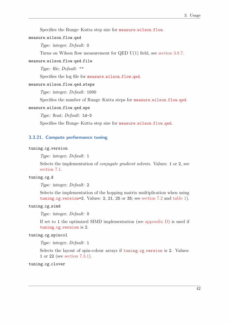
measure wilson flow
Type: integer; Default: 0
Turns on Wilson flow measurement for QCD SU(3) field, see section 3.8.6.
measure wilson flow file
Type: file; Default: ""
Specifies the log file for measure wilson flow.
measure wilson flow steps
Type: integer; Default: 1000
Specifies the number of Runge–Kutta steps for measure wilson flow.
measure wilson flow eps
Type: float; Default: 1d-3
41
3. Usage
Specifies the Runge–Kutta step size for measure wilson flow.
measure wilson flow qed
Type: integer; Default: 0
Turns on Wilson flow measurement for QED U(1) field, see section 3.8.7.
measure wilson flow qed file
Type: file; Default: ""
Specifies the log file for measure wilson flow qed.
measure wilson flow qed steps
Type: integer; Default: 1000
Specifies the number of Runge–Kutta steps for measure wilson flow qed.
measure wilson flow qed eps
Type: float; Default: 1d-3
Specifies the Runge–Kutta step size for measure wilson flow qed.
3.3.21. Compute performance tuning
tuning cg version
Type: integer; Default: 1
Selects the implementation of conjugate gradient solvers. Values: 1 or 2, seesection 7.1.
tuning cg d
Type: integer; Default: 2
Selects the implementation of the hopping matrix multiplication when usingtuning cg version=2. Values: 2, 21, 25 or 35; see section 7.2 and table 1).
tuning cg simd
Type: integer; Default: 0
If set to 1 the optimized SIMD implementation (see appendix D) is used iftuning cg version is 2.
tuning cg spincol
Type: integer; Default: 1
Selects the layout of spin-colour arrays if tuning cg version is 2. Values:1 or 22 (see section 7.3.1).
tuning cg clover
42
3. Usage
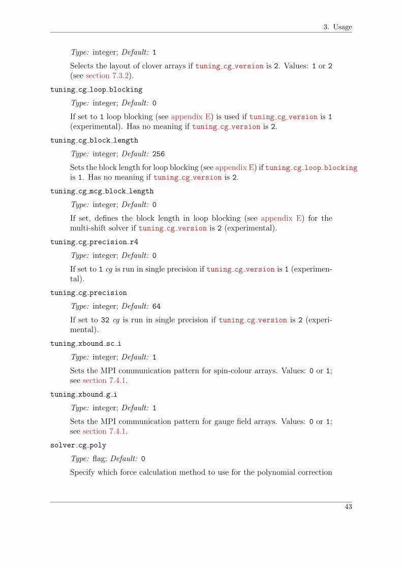
Type: integer; Default: 1
Selects the layout of clover arrays if tuning cg version is 2. Values: 1 or 2(see section 7.3.2).
tuning cg loop blocking
Type: integer; Default: 0
If set to 1 loop blocking (see appendix E) is used if tuning cg version is 1(experimental). Has no meaning if tuning cg version is 2.
tuning cg block length
Type: integer; Default: 256
Sets the block length for loop blocking (see appendix E) if tuning cg loop blocking
is 1. Has no meaning if tuning cg version is 2.
tuning cg mcg block length
Type: integer; Default: 0
If set, defines the block length in loop blocking (see appendix E) for themulti-shift solver if tuning cg version is 2 (experimental).
tuning cg precision r4
Type: integer; Default: 0
If set to 1 cg is run in single precision if tuning cg version is 1 (experimen-tal).
tuning cg precision
Type: integer; Default: 64
If set to 32 cg is run in single precision if tuning cg version is 2 (experi-mental).
tuning xbound sc i
Type: integer; Default: 1
Sets the MPI communication pattern for spin-colour arrays. Values: 0 or 1;see section 7.4.1.
tuning xbound g i
Type: integer; Default: 1
Sets the MPI communication pattern for gauge field arrays. Values: 0 or 1;see section 7.4.1.
solver cg poly
Type: flag; Default: 0
Specify which force calculation method to use for the polynomial correction
43
3. Usage
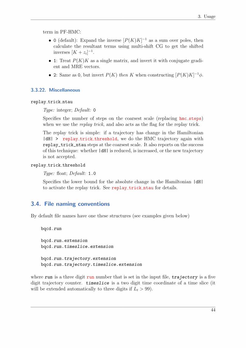
term in PF-HMC:
• 0 (default): Expand the inverse [P (K)K]−1 as a sum over poles, thencalculate the resultant terms using multi-shift CG to get the shiftedinverses [K + zi]
−1.
• 1: Treat P (K)K as a single matrix, and invert it with conjugate gradi-ent and MRE vectors.
• 2: Same as 0, but invert P (K) then K when constructing [P (K)K]−1φ.
3.3.22. Miscellaneous
replay trick ntau
Type: integer; Default: 0
Specifies the number of steps on the coarsest scale (replacing hmc steps)when we use the replay trick, and also acts as the flag for the replay trick.
The replay trick is simple: if a trajectory has change in the Hamiltonian|dH| > replay trick threshold, we do the HMC trajectory again withreplay_trick_ntau steps at the coarsest scale. It also reports on the successof this technique: whether |dH| is reduced, is increased, or the new trajectoryis not accepted.
replay trick threshold
Type: float; Default: 1.0
Specifies the lower bound for the absolute change in the Hamiltonian |dH|
to activate the replay trick. See replay trick ntau for details.
3.4. File naming conventions
By default file names have one these structures (see examples given below)
bqcd.run
bqcd.run.extension
bqcd.run.timeslice.extension
bqcd.run.trajectory.extension
bqcd.run.trajectory.timeslice.extension
where run is a three digit run number that is set in the input file, trajectory is a fivedigit trajectory counter. timeslice is a two digit time coordinate of a time slice (itwill be extended automatically to three digits if Lt > 99).
44

3. Usage
extension is set by the program for bqcd and bqcd2 formats, for the ildg format itcan be set by the ildg filename extension input parameter.
Output formats are described in section 6.7.
3.4.1. input, output and batch log files
These file names are not automatically being generated by the program. We choosenames that fit to the naming scheme:
bqcd.200 input (command line parameter)bqcd.200.res output (command line parameter)bqcd.200.input input (command line parameter)bqcd.200.output output (command line parameter)bqcd.200.log log file from batch system
3.4.2. Restart files in bqcd format
bqcd.200.count counters: run, job, trajectory
bqcd.200.info configuration metadatabqcd.200.ran state of random number generatorbqcd.200.00.u timeslice 0 of SU(3) configurationbqcd.200.01.u timeslice 1, . . .bqcd.200.02.u
bqcd.200.03.u
3.4.3. Restart files in bqcd2 format
bqcd.200.count counters: run, job, trajectory
bqcd.200.info configuration metadatabqcd.200.ran state of random number generatorbqcd.200.su3 SU(3) configuration
3.4.4. Restart files in lime format
bqcd.200.lime all restart information
3.4.5. Configuration files in bqcd format
bqcd.200.00010.info configuration metadatabqcd.200.00010.00.u configuration at trajectory 10, timeslice 0bqcd.200.00010.01.u configuration at trajectory 10, timeslice 1
45

3. Usage
bqcd.200.00010.02.u . . .bqcd.200.00010.03.u
3.4.6. Configuration files in bqcd2 format
bqcd.200.00010.info configuration metadatabqcd.200.00010.su3 configuration at trajectory 10
3.4.7. Configuration files in ildg format
bqcd.200.xml ensemble metadatabqcd.200.00010.xml metadata of configuration at trajectory 10bqcd.200.00010.lime binary data of configuration at trajectory 10
3.5. Flexible filenames
The advantage of the default filenames described in section 3.4 is that the names areshort. However, many users prefer to put characteristic metadata into filenames (e.g. β,κ and the lattice size).
The following macros can be used in filename specifications:
macro replacement%BE beta
%KL nf2 kappa1
%KS nf1 kappa1
%LL nf2 lambda1
%LS nf1 lambda1
%LX lattice(1)
%LY lattice(2)
%LZ lattice(3)
%LT lattice(4)
%Rn run (n = 1..9 digits)%Tn trajectory counter (n = 1..9 digits)
The macros can be used with these input parameters:
io bqcd restart filename
io bqcd conf filename
ildg filename prefix
ildg filename middle
3.6. Working with data in ILDG format
46
3. Usage
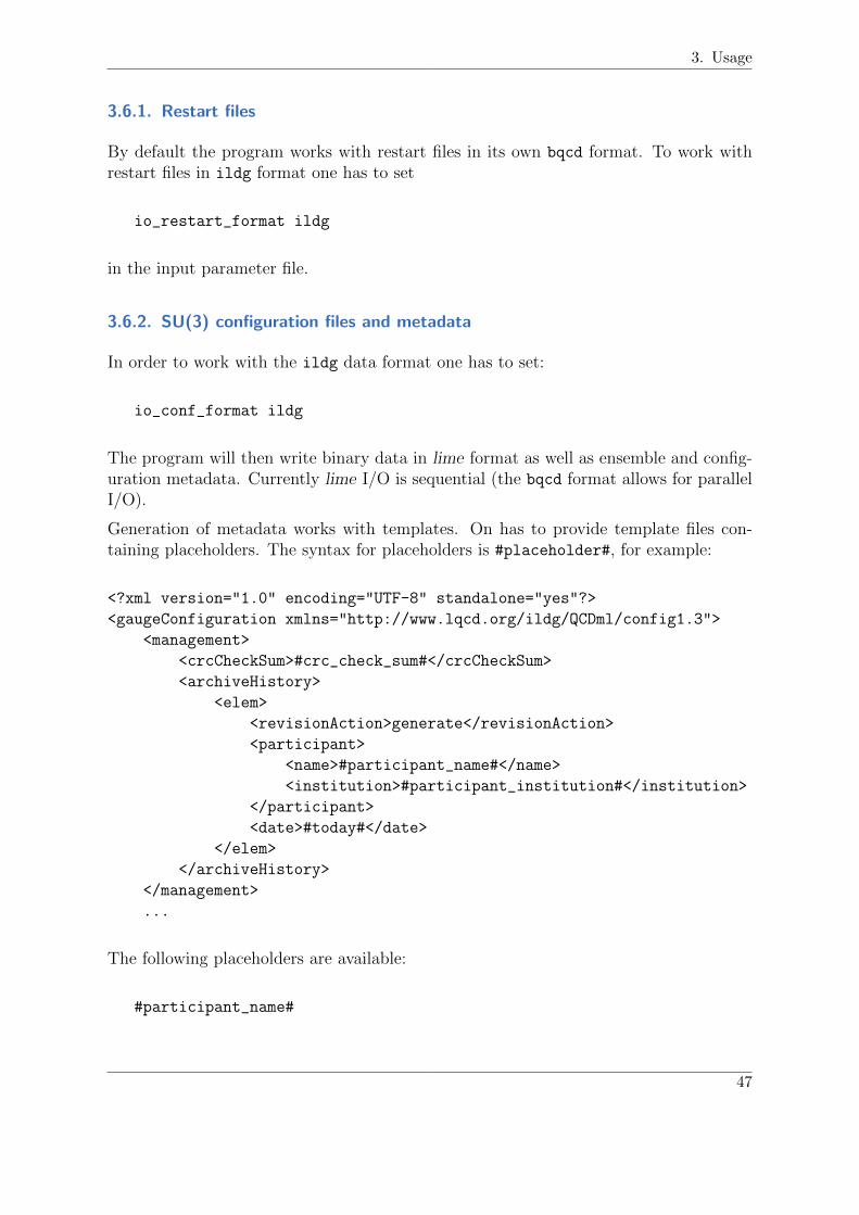
3.6.1. Restart files
By default the program works with restart files in its own bqcd format. To work withrestart files in ildg format one has to set
io_restart_format ildg
in the input parameter file.
3.6.2. SU(3) configuration files and metadata
In order to work with the ildg data format one has to set:
io_conf_format ildg
The program will then write binary data in lime format as well as ensemble and config-uration metadata. Currently lime I/O is sequential (the bqcd format allows for parallelI/O).
Generation of metadata works with templates. On has to provide template files con-taining placeholders. The syntax for placeholders is #placeholder#, for example:
<?xml version="1.0" encoding="UTF-8" standalone="yes"?>
<gaugeConfiguration xmlns="http://www.lqcd.org/ildg/QCDml/config1.3">
<management>
<crcCheckSum>#crc_check_sum#</crcCheckSum>
<archiveHistory>
<elem>
<revisionAction>generate</revisionAction>
<participant>
<name>#participant_name#</name>
<institution>#participant_institution#</institution>
</participant>
<date>#today#</date>
</elem>
</archiveHistory>
</management>
...
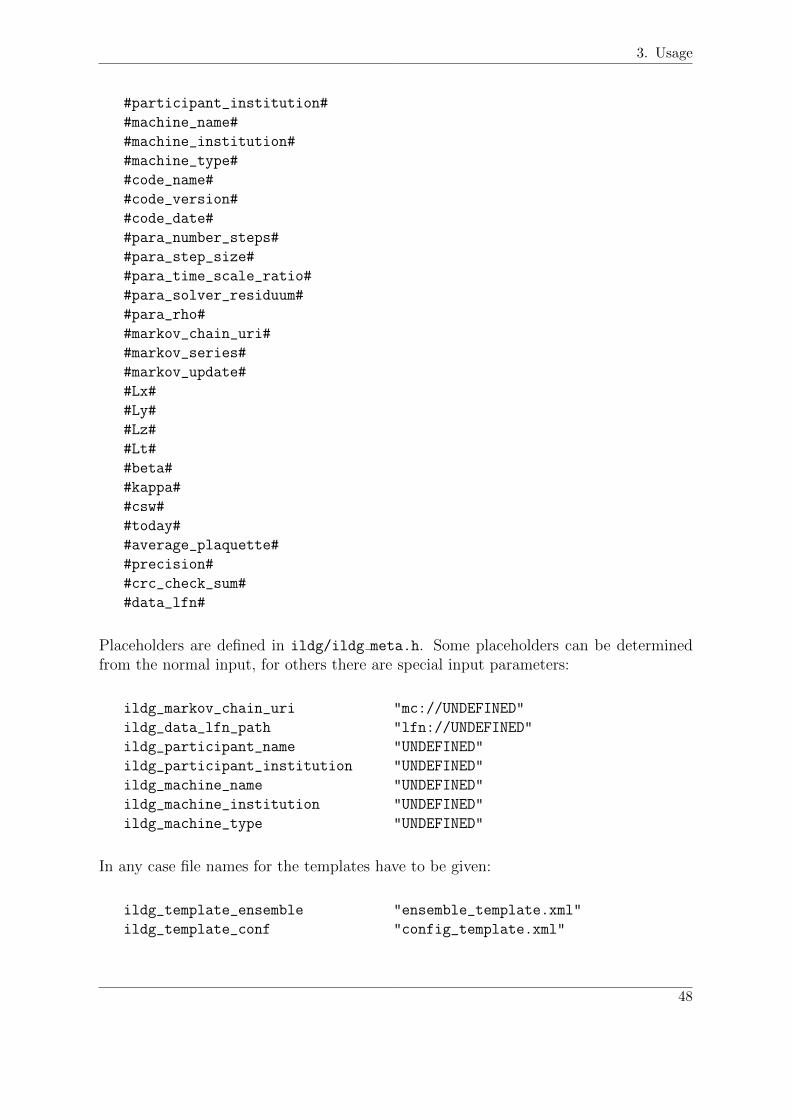
The following placeholders are available:
#participant_name#
47
3. Usage
#participant_institution#
#machine_name#
#machine_institution#
#machine_type#
#code_name#
#code_version#
#code_date#
#para_number_steps#
#para_step_size#
#para_time_scale_ratio#
#para_solver_residuum#
#para_rho#
#markov_chain_uri#
#markov_series#
#markov_update#
#Lx#
#Ly#
#Lz#
#Lt#
#beta#
#kappa#
#csw#
#today#
#average_plaquette#
#precision#
#crc_check_sum#
#data_lfn#
Placeholders are defined in ildg/ildg meta.h. Some placeholders can be determinedfrom the normal input, for others there are special input parameters:
ildg_markov_chain_uri "mc://UNDEFINED"
ildg_data_lfn_path "lfn://UNDEFINED"
ildg_participant_name "UNDEFINED"
ildg_participant_institution "UNDEFINED"
ildg_machine_name "UNDEFINED"
ildg_machine_institution "UNDEFINED"
ildg_machine_type "UNDEFINED"
In any case file names for the templates have to be given:
ildg_template_ensemble "ensemble_template.xml"
ildg_template_conf "config_template.xml"
48

3. Usage
One can also set prefix and extension of the ildg files:
ildg_filename_prefix "qcdsf.%R3"
ildg_filename_extension "lime"
This setting would, for example, generate these configuration files:
qcdsf.200.xml
qcdsf.200.00010.xml
qcdsf.200.00010.lime
3.6.3. Precision
The program can handle ildg files in 32- and 64-bit precision. When reading theprecision is taken from the ildg file. The precision of writing can be set to 32-bit by:
ildg_precision 32 SU(3) configurationsildg_precision_restart 32 restart files (for testing)
3.6.4. Example of a complete set of ildg settings
io_conf_format "ildg"
ildg_filename_prefix "qcdsf.%R3"
ildg_filename_extension "lime"
ildg_precision 64
ildg_template_ensemble "../data/qcdsf-ensemble-05.xml"
ildg_template_conf "../data/qcdsf-configuration-05.xml"
ildg_markov_chain_uri "mc://ldg/qcdsf/clover_nf2/b5p00kp13000-04x04"
ildg_data_lfn_path "lfn://ldg/qcdsf/clover_nf2/b5p00kp13000-04x04"
ildg_participant_name "Hinnerk Stueben"
ildg_participant_institution "Universitaet Hamburg"
ildg_machine_name "HLRN-III"
ildg_machine_institution "HLRN"
ildg_machine_type "Cray XC40"
3.7. Output – structure of res(ults) file
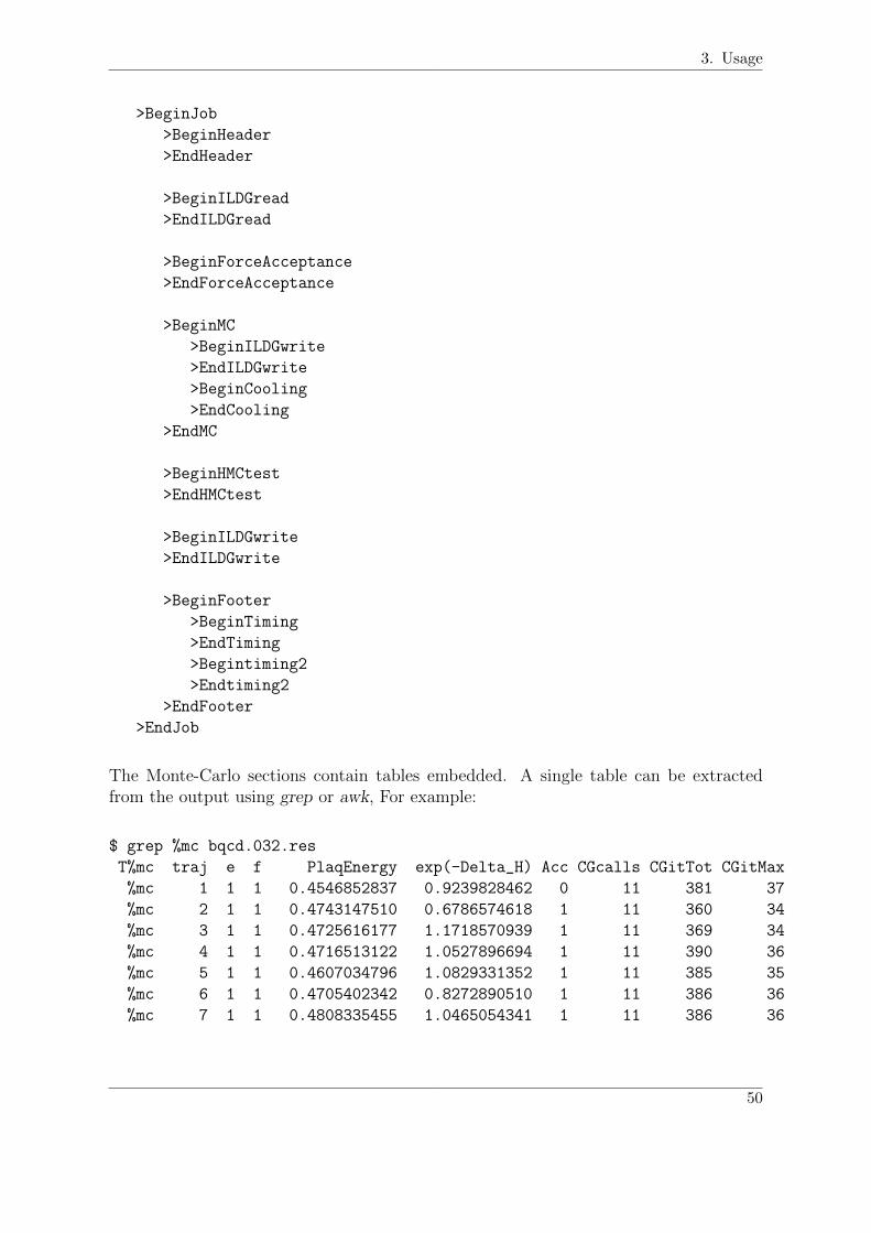
The output was structured in such a way that it is humanly readable and can be easilyprocessed with awk. As a consequence each line begins with a keyword which is followedby data. In addition there are sections. The sections are:
49
3. Usage
>BeginJob
>BeginHeader
>EndHeader
>BeginILDGread
>EndILDGread
>BeginForceAcceptance
>EndForceAcceptance
>BeginMC
>BeginILDGwrite
>EndILDGwrite
>BeginCooling
>EndCooling
>EndMC
>BeginHMCtest
>EndHMCtest
>BeginILDGwrite
>EndILDGwrite
>BeginFooter
>BeginTiming
>EndTiming
>Begintiming2
>Endtiming2
>EndFooter
>EndJob
The Monte-Carlo sections contain tables embedded. A single table can be extractedfrom the output using grep or awk, For example:
$ grep %mc bqcd.032.res
T%mc traj e f PlaqEnergy exp(-Delta_H) Acc CGcalls CGitTot CGitMax
%mc 1 1 1 0.4546852837 0.9239828462 0 11 381 37
%mc 2 1 1 0.4743147510 0.6786574618 1 11 360 34
%mc 3 1 1 0.4725616177 1.1718570939 1 11 369 34
%mc 4 1 1 0.4716513122 1.0527896694 1 11 390 36
%mc 5 1 1 0.4607034796 1.0829331352 1 11 385 35
%mc 6 1 1 0.4705402342 0.8272890510 1 11 386 36
%mc 7 1 1 0.4808335455 1.0465054341 1 11 386 36
50
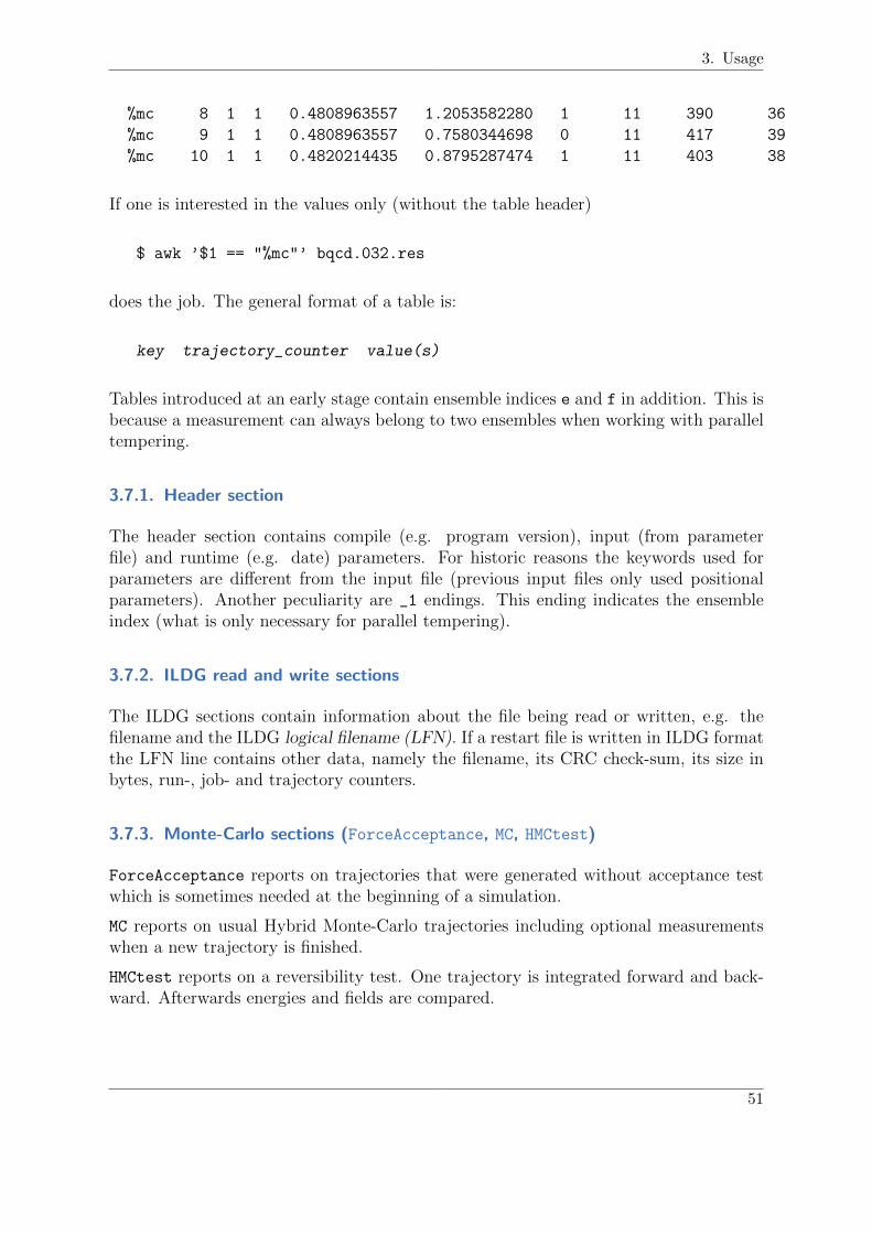
3. Usage
%mc 8 1 1 0.4808963557 1.2053582280 1 11 390 36
%mc 9 1 1 0.4808963557 0.7580344698 0 11 417 39
%mc 10 1 1 0.4820214435 0.8795287474 1 11 403 38
If one is interested in the values only (without the table header)
$ awk ’$1 == "%mc"’ bqcd.032.res
does the job. The general format of a table is:
key trajectory_counter value(s)
Tables introduced at an early stage contain ensemble indices e and f in addition. This isbecause a measurement can always belong to two ensembles when working with paralleltempering.
3.7.1. Header section
The header section contains compile (e.g. program version), input (from parameterfile) and runtime (e.g. date) parameters. For historic reasons the keywords used forparameters are different from the input file (previous input files only used positionalparameters). Another peculiarity are _1 endings. This ending indicates the ensembleindex (what is only necessary for parallel tempering).
3.7.2. ILDG read and write sections
The ILDG sections contain information about the file being read or written, e.g. thefilename and the ILDG logical filename (LFN). If a restart file is written in ILDG formatthe LFN line contains other data, namely the filename, its CRC check-sum, its size inbytes, run-, job- and trajectory counters.
3.7.3. Monte-Carlo sections (ForceAcceptance, MC, HMCtest)
ForceAcceptance reports on trajectories that were generated without acceptance testwhich is sometimes needed at the beginning of a simulation.
MC reports on usual Hybrid Monte-Carlo trajectories including optional measurementswhen a new trajectory is finished.
HMCtest reports on a reversibility test. One trajectory is integrated forward and back-ward. Afterwards energies and fields are compared.
51

3. Usage
3.7.4. Cooling section
This section contains a cooling history with the measurement of the topological charge.
3.7.5. Footer section
In the footer one finds the end of execution date, the elapsed run time and how manyCPUs were used (#CPUs = #cores = MPI processes × OpenMP threads).
3.7.6. Timing sections
Output from profiling. Results are shown in a table that list how often a region wascalled and how much time was spent in that region:
Performance
region #calls time mean min max Total
s Mflop/s Mflop/s Mflop/s Gflop/s
For the most interesting regions the number of floating point were counted. In thesecases the table lists the average, minimal and maximal performance per CPU (core) aswell as the overall performance.
52

3. Usage
3.7.7. List of embedded tables
key meaning%fa forced acceptance logs%mc main Hybrid Monte-Carlo logs%pr rectangular plaquettes%Hold energies at start of trajectory%Hnew energies at end of trajectory%Hdif energy differences (∆H)%Favg average forces in molecular dynamics integration%Fmax maximal forces in molecular dynamics integration%Frat force ratios: maximal forces / minimal forces%Frac forces in RHMC molecular dynamics integration%Qc topological charge from cooling (cooling history)%pl Polyakov loop%tr fermionic bulk quantities (traces)%it counters of cg iterations%it4 counters of cg32 bit iterations%cgChk check of cg solution%bicgstabChk check of Bicgstab solution%bicgstabmixChk check of mixed precision Bicgstab solution%cg_ritz check of Ritz cg solution%cg_ritz_dd check of Ritz cg solution%shift check of multi shift solutions%egnv eigenvalues
3.8. Measurements
Measurements are made at the end of every trajectory.
3.8.1. Topological charge
To measure the topological charge with the cooling method a file must be provided inwhich the cooling steps are defined. One has to set
measure cooling list filename
in the input file. The file contains the cooling steps after which the topological chargeand the plaquette are measured. For example,
1
2
5
10
53

3. Usage
20
In this case 20 cooling iterations are made and measurements are performed after coolingiteration 1, 2, 5, 10 and 20. The corresponding output looks like this:
>BeginCooling
T%Qc traj e f i_cool Q_cool PlaqEnergy
%Qc 1 1 1 1 -0.137916 0.3552673573
%Qc 1 1 1 2 -0.347026 0.1878487312
%Qc 1 1 1 5 -0.650364 0.0555456917
%Qc 1 1 1 10 -0.533735 0.0181235629
%Qc 1 1 1 20 0.000154 0.0051610597
>EndCooling
3.8.2. Polyakov loop
To measure the Polyakov loop, set
measure polyakov loop 1
in the input file.
3.8.3. Fermionic bulk quantities
To measure fermionic bulk quantities, set non zero value
measure traces 1
in the input file. The value is number of noises. You can specify the file log of thesemeasurements by measure traces file. The corresponding outputs are summarized in%tr, %trd and %trm.
Traces up to fourth derivative are labeled as:
Tabcd =1
12N3sNt
Tr(MaMbMcMd) (3)
where a, b, c, d = 0, 1, 2, 3 and
M0 = 1
M1 = D−1
M2 =(∂D∂µ
)D−1
M3 =(∂2D∂µ2
)D−1
(4)
54
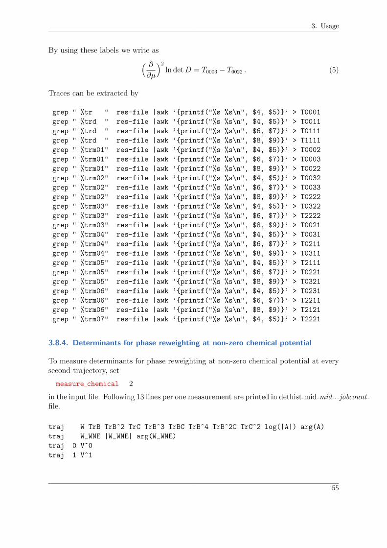
3. Usage
By using these labels we write as( ∂∂µ
)2ln detD = T0003 − T0022 . (5)
Traces can be extracted by
grep " %tr " res-file |awk ’{printf("%s %s\n", $4, $5)}’ > T0001
grep " %trd " res-file |awk ’{printf("%s %s\n", $4, $5)}’ > T0011
grep " %trd " res-file |awk ’{printf("%s %s\n", $6, $7)}’ > T0111
grep " %trd " res-file |awk ’{printf("%s %s\n", $8, $9)}’ > T1111
grep " %trm01" res-file |awk ’{printf("%s %s\n", $4, $5)}’ > T0002
grep " %trm01" res-file |awk ’{printf("%s %s\n", $6, $7)}’ > T0003
grep " %trm01" res-file |awk ’{printf("%s %s\n", $8, $9)}’ > T0022
grep " %trm02" res-file |awk ’{printf("%s %s\n", $4, $5)}’ > T0032
grep " %trm02" res-file |awk ’{printf("%s %s\n", $6, $7)}’ > T0033
grep " %trm02" res-file |awk ’{printf("%s %s\n", $8, $9)}’ > T0222
grep " %trm03" res-file |awk ’{printf("%s %s\n", $4, $5)}’ > T0322
grep " %trm03" res-file |awk ’{printf("%s %s\n", $6, $7)}’ > T2222
grep " %trm03" res-file |awk ’{printf("%s %s\n", $8, $9)}’ > T0021
grep " %trm04" res-file |awk ’{printf("%s %s\n", $4, $5)}’ > T0031
grep " %trm04" res-file |awk ’{printf("%s %s\n", $6, $7)}’ > T0211
grep " %trm04" res-file |awk ’{printf("%s %s\n", $8, $9)}’ > T0311
grep " %trm05" res-file |awk ’{printf("%s %s\n", $4, $5)}’ > T2111
grep " %trm05" res-file |awk ’{printf("%s %s\n", $6, $7)}’ > T0221
grep " %trm05" res-file |awk ’{printf("%s %s\n", $8, $9)}’ > T0321
grep " %trm06" res-file |awk ’{printf("%s %s\n", $4, $5)}’ > T0231
grep " %trm06" res-file |awk ’{printf("%s %s\n", $6, $7)}’ > T2211
grep " %trm06" res-file |awk ’{printf("%s %s\n", $8, $9)}’ > T2121
grep " %trm07" res-file |awk ’{printf("%s %s\n", $4, $5)}’ > T2221
3.8.4. Determinants for phase reweighting at non-zero chemical potential
To measure determinants for phase reweighting at non-zero chemical potential at everysecond trajectory, set
measure chemical 2
in the input file. Following 13 lines per one measurement are printed in dethist.mid mid . jobcountfile.
traj W TrB TrB^2 TrC TrB^3 TrBC TrB^4 TrB^2C TrC^2 log(|A|) arg(A)
traj W_WNE |W_WNE| arg(W_WNE)
traj 0 V^0
traj 1 V^1
55

3. Usage
traj 2 ...
traj 3 ...
traj 4 ...
traj 5 ...
traj 6 ...
traj 7 ...
traj 9 ...
traj 10 ...
where W is det(K), B is K, C is K, A is A0. 2nd line is
WWNE = exp[−
10∑q=1
(2 cosh(qµ/T )ReV (q) + i2 sinh(qµ/T )ImV (q))]
(6)
and its absolute value and argument. From 3rd line V (q) are printed for each trace. Eachvalue is defined in Ref. [40].
3.8.5. fA and fP
To measure fA and fP for non-perturbative determination of cSW at every second tra-jectory, set
measure schrpcac 2
in the input file. The corresponding output looks like this:
traj t+1 fA(t) fP(t) fA’(T-t) fP’(T-t)
2 2 -0.10939226E+02 0.32266553E+02 -0.56909470E+01 0.17781391E+02
2 3 -0.34826553E+01 0.87987951E+01 -0.19998378E+01 0.40562673E+01
2 4 -0.10307930E+01 0.19997526E+01 -0.87475663E+00 0.11811545E+01
4 2 -0.10427659E+02 0.36927566E+02 -0.57629684E+01 0.18859736E+02
4 3 -0.49157290E+01 0.13352503E+02 -0.31013816E+01 0.54608054E+01
4 4 -0.19897425E+01 0.38296835E+01 -0.18940843E+01 0.23258797E+01
3.8.6. Wilson flow for QCD field
To measure Wilson flow for QCD field at every second trajectory, set
measure wilson flow 2
in the input file. The corresponding output looks like this (12 digits are printed in actualoutput):
traj, t, Ep(t), Ec(t), Ec(t)t^2, t* dt Ec(t)^2, Qtop, (1-Ep(t))t^2
56

3. Usage
0 0.00E+00 0.22E+00 0.22E+01 0.00E+00 0.00E+00 -0.91E-01 0.00E+00
0 0.10E-01 0.25E+00 0.22E+01 0.22E-03 0.22E-03 -0.96E-01 0.74E-04
0 0.20E-01 0.27E+00 0.23E+01 0.93E-03 0.14E-02 -0.10E+00 0.29E-03
0 0.30E-01 0.29E+00 0.23E+01 0.21E-02 0.35E-02 -0.10E+00 0.63E-03
where t is flow time, Ep(t) is plaquette energy, Ec(t) is clover energy and Qtop istopological charge.
3.8.7. Wilson flow for QED field
To measure Wilson flow for QED field at every second trajectory, set
measure wilson flow qed 2
in the input file. The corresponding output is same format as Wilson flow for QCDfield.
57
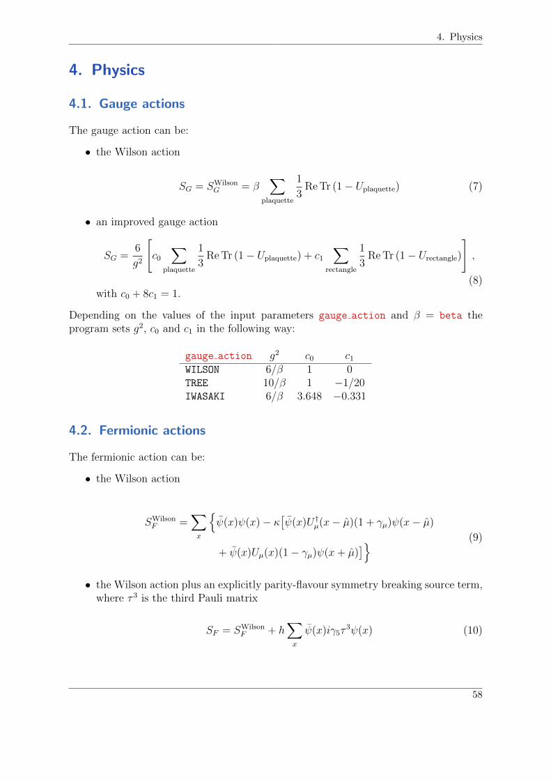
4. Physics
4. Physics
4.1. Gauge actions
The gauge action can be:
• the Wilson action
SG = SWilsonG = β
∑plaquette
1
3Re Tr (1− Uplaquette) (7)
• an improved gauge action
SG =6
g2
[c0
∑plaquette
1
3Re Tr (1− Uplaquette) + c1
∑rectangle
1
3Re Tr (1− Urectangle)
],
(8)with c0 + 8c1 = 1.
Depending on the values of the input parameters gauge action and β = beta theprogram sets g2, c0 and c1 in the following way:
gauge action g2 c0 c1WILSON 6/β 1 0TREE 10/β 1 −1/20IWASAKI 6/β 3.648 −0.331
4.2. Fermionic actions
The fermionic action can be:
• the Wilson action
SWilsonF =
∑x
{ψ(x)ψ(x)− κ
[ψ(x)U †µ(x− µ)(1 + γµ)ψ(x− µ)
+ ψ(x)Uµ(x)(1− γµ)ψ(x+ µ)]} (9)
• the Wilson action plus an explicitly parity-flavour symmetry breaking source term,where τ 3 is the third Pauli matrix
SF = SWilsonF + h
∑x
ψ(x)iγ5τ3ψ(x) (10)
58
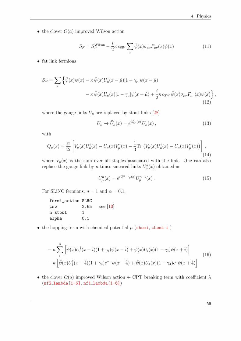
4. Physics
• the clover O(a) improved Wilson action
SF = SWilsonF − i
2κ cSW
∑x
ψ(x)σµνFµν(x)ψ(x) (11)
• fat link fermions
SF =∑x
{ψ(x)ψ(x)− κ ψ(x)U †µ(x− µ)[1 + γµ]ψ(x− µ)
− κ ψ(x)Uµ(x)[1− γµ]ψ(x+ µ) +i
2κ cSW ψ(x)σµνFµν(x)ψ(x)
},
(12)
where the gauge links Uµ are replaced by stout links [28]
Uµ → Uµ(x) = eiQµ(x) Uµ(x) , (13)
with
Qµ(x) =α
2i
[Vµ(x)U †µ(x)− Uµ(x)V †µ (x)− 1
3Tr(Vµ(x)U †µ(x)− Uµ(x)V †µ (x)
)],
(14)where Vµ(x) is the sum over all staples associated with the link. One can alsoreplace the gauge link by n times smeared links Un
µ (x) obtained as
Unµ (x) = eiQ
n−1µ(x)Un−1
µ (x) . (15)
For SLiNC fermions, n = 1 and α = 0.1,
fermi_action SLRC
csw 2.65 see [10]n_stout 1
alpha 0.1
• the hopping term with chemical potential µ (chemi, chemi i )
− κ3∑i
[ψ(x)U †i (x− i)(1 + γi)ψ(x− i) + ψ(x)Ui(x)(1− γi)ψ(x+ i)
]− κ
[ψ(x)U †4(x− 4)(1 + γ4)e
−µψ(x− 4) + ψ(x)U4(x)(1− γ4)eµψ(x+ 4)] (16)
• the clover O(a) improved Wilson action + CPT breaking term with coefficient λ(nf2 lambda[1-6], nf1 lambda[1-6])
59
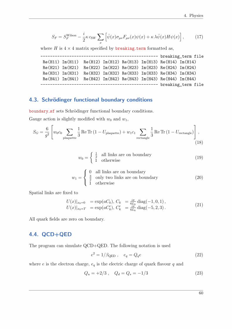
4. Physics
SF = SWilsonF − i
2κ cSW
∑x
[ψ(x)σµνFµν(x)ψ(x) + κλψ(x)Hψ(x)
], (17)
where H is 4× 4 matrix specified by breaking term formatted as,
------------------------------------------------- breaking_term file
Re(H11) Im(H11) Re(H12) Im(H12) Re(H13) Im(H13) Re(H14) Im(H14)
Re(H21) Im(H21) Re(H22) Im(H22) Re(H23) Im(H23) Re(H24) Im(H24)
Re(H31) Im(H31) Re(H32) Im(H32) Re(H33) Im(H33) Re(H34) Im(H34)
Re(H41) Im(H41) Re(H42) Im(H42) Re(H43) Im(H43) Re(H44) Im(H44)
------------------------------------------------- breaking_term file
4.3. Schrodinger functional boundary conditions
boundary sf sets Schrodinger functional boundary conditions.
Gauge action is slightly modified with w0 and w1,
SG =6
g2
[w0c0
∑plaquette
1
3Re Tr (1− Uplaquette) + w1c1
∑rectangle
1
3Re Tr (1− Urectangle)
],
(18)
w0 =
{12
all links are on boundary1 otherwise
(19)
w1 =
0 all links are on boundary32
only two links are on boundary1 otherwise
(20)
Spatial links are fixed to
U(x)|x0=0 = exp(aCk), Ck = iπ6Lk
diag(−1, 0, 1) ,
U(x)|x0=T = exp(aC ′k), C′k = iπ
6Lkdiag(−5, 2, 3) .
(21)
All quark fields are zero on boundary.
4.4. QCD+QED
The program can simulate QCD+QED. The following notation is used
e2 = 1/βQED , eq = Qqe (22)
where e is the electron charge, eq is the electric charge of quark flavour q and
Qu = +2/3 , Qd = Qs = −1/3 (23)
60

4. Physics
for the the up, down and strange quark respectively.
The following actions can be simulated:
S = SG + SA +∑q
SqF . (24)
SG is an SU(3) gauge action, SA is the non-compact U(1) gauge action
SA =βQED
2
∑x,µ<ν
[Aµ(x) + Aν(x+ µ)− Aµ(x+ ν)− Aν(x)]2 , (25)
and the fermion action for flavour q is
SqF =∑x
{1
2
∑µ
[q(x)(γµ − 1)e−iQqAµ(x)Uµ(x)q(x+ µ)
−q(x)(γµ + 1)eiQqAµ(x−µ)U †µ(x− µ)q(x− µ)]
+1
2κqq(x)q(x)− 1
4cSW
∑µ,ν
q(x)σµνFµν(x)q(x)
}, (26)
where Uµ is a singly iterated stout link (see eq. (13)). The clover coefficient cSW wascomputed non-perturbatively in pure QCD in [38].
The corresponding input keywords are beta qed, nf2 em charge[1-6] x3 andnf1 em charge[1-6] x3.
4.5. Axion
The program can simulate QCD+Axion. The following actions an be simulated:
S = SG + Sa +∑q
SqF . (27)
Sa is the scalar action
Sa = κa∑x
∑µ
(φa(x)− φa(x+ µ)
)φa(x) , (28)
where φa is the axion field. The fermion action for flavour q in the case of Wilsonfermions is
SqF =∑x
q(x)[1 + (κqλq + finvφa)γ5
]q(x)
− κq∑x,µ
[q(x)(1− γµ)Uµ(x)q(x+ aµ) + q(x− aµ)(1 + γµ)U †µ(x− aµ)q(x)
],
(29)
61
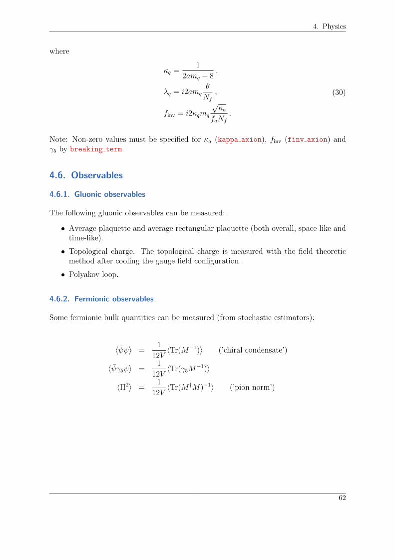
4. Physics
where
κq =1
2amq + 8,
λq = i2amqθ
Nf
,
finv = i2κqmq
√κa
faNf
.
(30)
Note: Non-zero values must be specified for κa (kappa axion), finv (finv axion) andγ5 by breaking term.
4.6. Observables
4.6.1. Gluonic observables
The following gluonic observables can be measured:
• Average plaquette and average rectangular plaquette (both overall, space-like andtime-like).
• Topological charge. The topological charge is measured with the field theoreticmethod after cooling the gauge field configuration.
• Polyakov loop.
4.6.2. Fermionic observables
Some fermionic bulk quantities can be measured (from stochastic estimators):
〈ψψ〉 =1
12V〈Tr(M−1)〉 (’chiral condensate’)
〈ψγ5ψ〉 =1
12V〈Tr(γ5M
−1)〉
〈Π2〉 =1
12V〈Tr(M †M)−1〉 (’pion norm’)
62
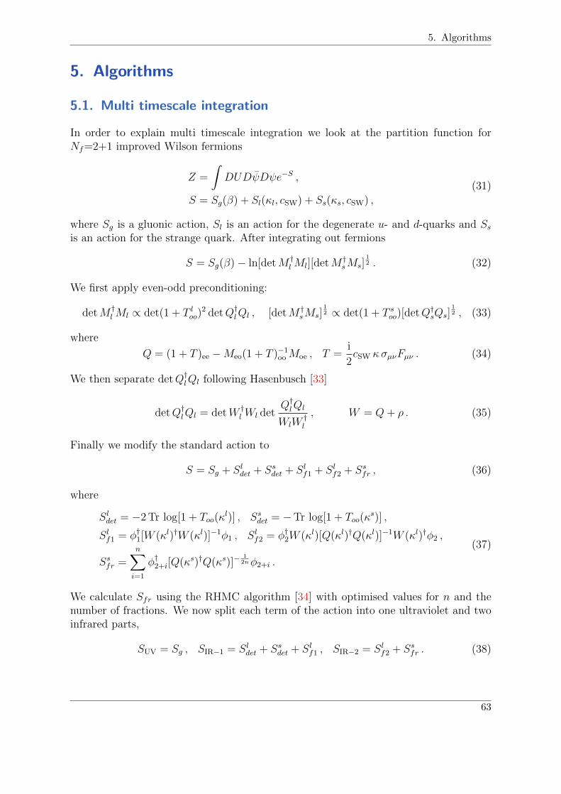
5. Algorithms
5. Algorithms
5.1. Multi timescale integration
In order to explain multi timescale integration we look at the partition function forNf=2+1 improved Wilson fermions
Z =
∫DUDψDψe−S ,
S = Sg(β) + Sl(κl, cSW) + Ss(κs, cSW) ,
(31)
where Sg is a gluonic action, Sl is an action for the degenerate u- and d-quarks and Ssis an action for the strange quark. After integrating out fermions
S = Sg(β)− ln[detM †lMl][detM †
sMs]12 . (32)
We first apply even-odd preconditioning:
detM †lMl ∝ det(1 + T loo)
2 detQ†lQl , [detM †sMs]
12 ∝ det(1 + T soo)[detQ†sQs]
12 , (33)
where
Q = (1 + T )ee −Meo(1 + T )−1ooMoe , T =i
2cSW κσµνFµν . (34)
We then separate detQ†lQl following Hasenbusch [33]
detQ†lQl = detW †l Wl det
Q†lQl
WlW†l
, W = Q+ ρ . (35)
Finally we modify the standard action to
S = Sg + Sldet + Ssdet + Slf1 + Slf2 + Ssfr , (36)
where
Sldet = −2 Tr log[1 + Too(κl)] , Ssdet = −Tr log[1 + Too(κ
s)] ,
Slf1 = φ†1[W (κl)†W (κl)]−1φ1 , Slf2 = φ†2W (κl)[Q(κl)†Q(κl)]−1W (κl)†φ2 ,
Ssfr =n∑i=1
φ†2+i[Q(κs)†Q(κs)]−12nφ2+i .
(37)
We calculate Sfr using the RHMC algorithm [34] with optimised values for n and thenumber of fractions. We now split each term of the action into one ultraviolet and twoinfrared parts,
SUV = Sg , SIR−1 = Sldet + Ssdet + Slf1 , SIR−2 = Slf2 + Ssfr . (38)
63
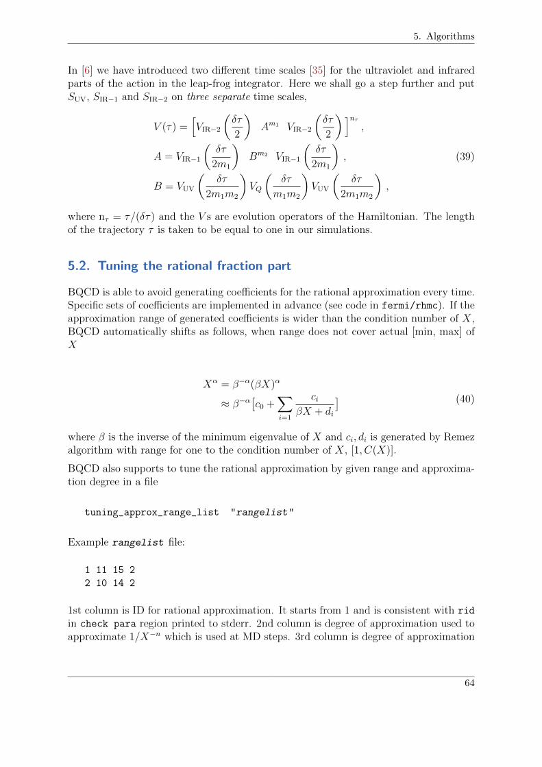
5. Algorithms
In [6] we have introduced two different time scales [35] for the ultraviolet and infraredparts of the action in the leap-frog integrator. Here we shall go a step further and putSUV, SIR−1 and SIR−2 on three separate time scales,
V (τ) =[VIR−2
(δτ
2
)Am1 VIR−2
(δτ
2
)]nτ,
A = VIR−1
(δτ
2m1
)Bm2 VIR−1
(δτ
2m1
),
B = VUV
(δτ
2m1m2
)VQ
(δτ
m1m2
)VUV
(δτ
2m1m2
),
(39)
where nτ = τ/(δτ) and the V s are evolution operators of the Hamiltonian. The lengthof the trajectory τ is taken to be equal to one in our simulations.
5.2. Tuning the rational fraction part
BQCD is able to avoid generating coefficients for the rational approximation every time.Specific sets of coefficients are implemented in advance (see code in fermi/rhmc). If theapproximation range of generated coefficients is wider than the condition number of X,BQCD automatically shifts as follows, when range does not cover actual [min, max] ofX
Xα = β−α(βX)α
≈ β−α[c0 +
∑i=1
ciβX + di
] (40)
where β is the inverse of the minimum eigenvalue of X and ci, di is generated by Remezalgorithm with range for one to the condition number of X, [1, C(X)].
BQCD also supports to tune the rational approximation by given range and approxima-tion degree in a file
tuning_approx_range_list "rangelist"
Example rangelist file:
1 11 15 2
2 10 14 2
1st column is ID for rational approximation. It starts from 1 and is consistent with rid
in check para region printed to stderr. 2nd column is degree of approximation used toapproximate 1/X−n which is used at MD steps. 3rd column is degree of approximation
64
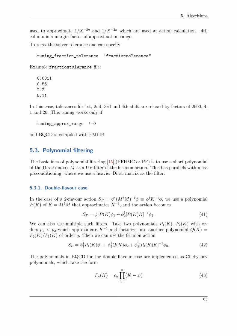
5. Algorithms
used to approximate 1/X−2n and 1/X+2n which are used at action calculation. 4thcolumn is a margin factor of approximation range.
To relax the solver tolerance one can specify
tuning_fraction_tolerance "fractiontolerance"
Example fractiontolerance file:
0.0011
0.55
2.2
0.11
In this case, tolerances for 1st, 2nd, 3rd and 4th shift are relaxed by factors of 2000, 4,1 and 20. This tuning works only if
tuning_approx_range !=0
and BQCD is compiled with FMLIB.
5.3. Polynomial filtering
The basic idea of polynomial filtering [15] (PFHMC or PF) is to use a short polynomialof the Dirac matrix M as a UV filter of the fermion action. This has parallels with masspreconditioning, where we use a heavier Dirac matrix as the filter.
5.3.1. Double-flavour case
In the case of a 2-flavour action SF = φ†(M †M)−1φ ≡ φ†K−1φ, we use a polynomialP (K) of K = M †M that approximates K−1, and the action becomes
SF = φ†1P (K)φ1 + φ†2[P (K)K]−1φ2. (41)
We can also use multiple such filters. Take two polynomials P1(K), P2(K) with or-ders p1 < p2 which approximate K−1 and factorize into another polynomial Q(K) =P2(K)/P1(K) of order q. Then we can use the fermion action
SF = φ†1P1(K)φ1 + φ†2Q(K)φ2 + φ†3[P3(K)K]−1φ3. (42)
The polynomials in BQCD for the double-flavour case are implemented as Chebyshevpolynomials, which take the form
Pn(K) = cn
n∏i=1
(K − zi) (43)
65
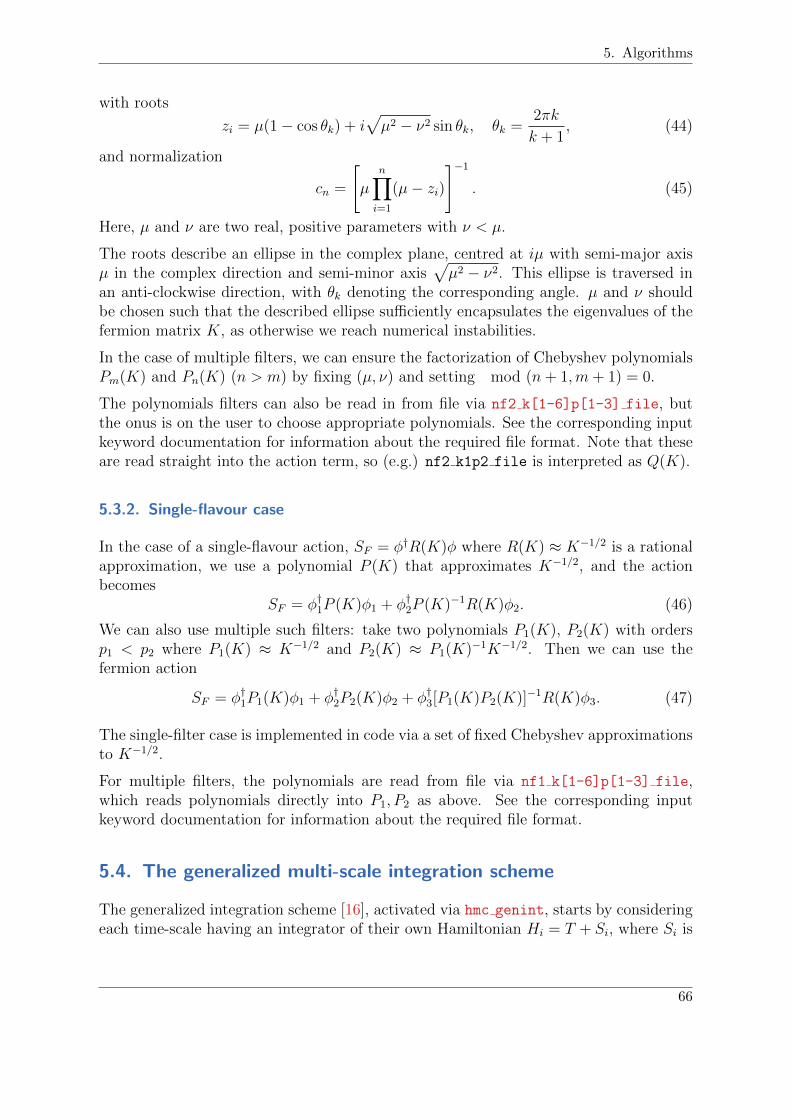
5. Algorithms
with roots
zi = µ(1− cos θk) + i√µ2 − ν2 sin θk, θk =
2πk
k + 1, (44)
and normalization
cn =
[µ
n∏i=1
(µ− zi)
]−1. (45)
Here, µ and ν are two real, positive parameters with ν < µ.
The roots describe an ellipse in the complex plane, centred at iµ with semi-major axisµ in the complex direction and semi-minor axis
√µ2 − ν2. This ellipse is traversed in
an anti-clockwise direction, with θk denoting the corresponding angle. µ and ν shouldbe chosen such that the described ellipse sufficiently encapsulates the eigenvalues of thefermion matrix K, as otherwise we reach numerical instabilities.
In the case of multiple filters, we can ensure the factorization of Chebyshev polynomialsPm(K) and Pn(K) (n > m) by fixing (µ, ν) and setting mod (n+ 1,m+ 1) = 0.
The polynomials filters can also be read in from file via nf2 k[1-6]p[1-3] file, butthe onus is on the user to choose appropriate polynomials. See the corresponding inputkeyword documentation for information about the required file format. Note that theseare read straight into the action term, so (e.g.) nf2 k1p2 file is interpreted as Q(K).
5.3.2. Single-flavour case
In the case of a single-flavour action, SF = φ†R(K)φ where R(K) ≈ K−1/2 is a rationalapproximation, we use a polynomial P (K) that approximates K−1/2, and the actionbecomes
SF = φ†1P (K)φ1 + φ†2P (K)−1R(K)φ2. (46)
We can also use multiple such filters: take two polynomials P1(K), P2(K) with ordersp1 < p2 where P1(K) ≈ K−1/2 and P2(K) ≈ P1(K)−1K−1/2. Then we can use thefermion action
SF = φ†1P1(K)φ1 + φ†2P2(K)φ2 + φ†3[P1(K)P2(K)]−1R(K)φ3. (47)
The single-filter case is implemented in code via a set of fixed Chebyshev approximationsto K−1/2.
For multiple filters, the polynomials are read from file via nf1 k[1-6]p[1-3] file,which reads polynomials directly into P1, P2 as above. See the corresponding inputkeyword documentation for information about the required file format.
5.4. The generalized multi-scale integration scheme
The generalized integration scheme [16], activated via hmc genint, starts by consideringeach time-scale having an integrator of their own Hamiltonian Hi = T + Si, where Si is
66
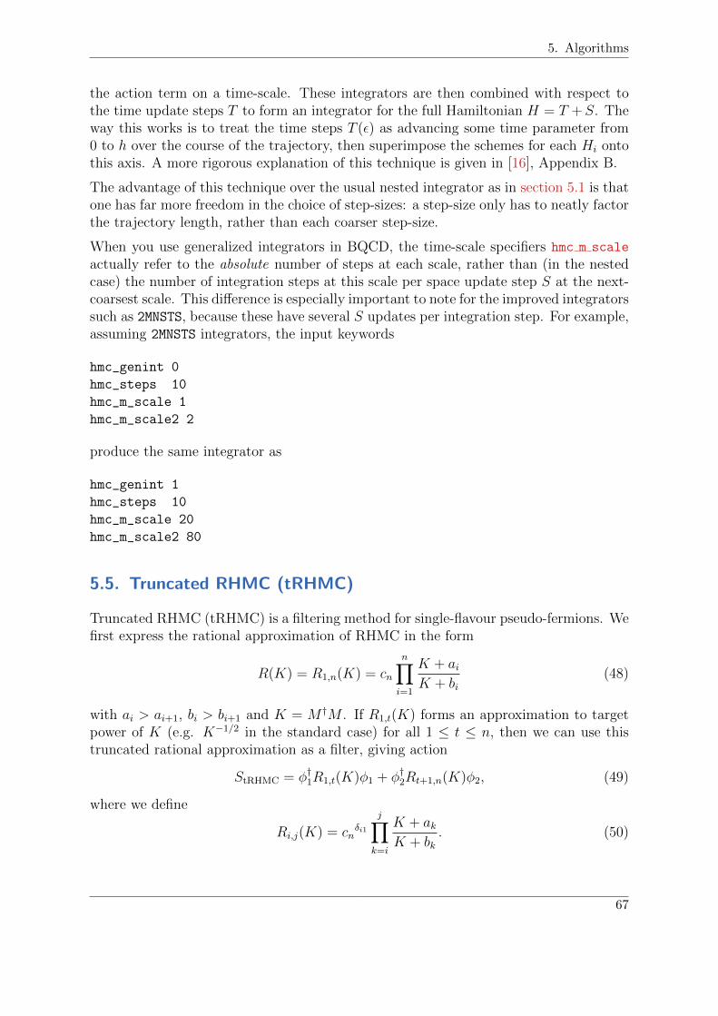
5. Algorithms
the action term on a time-scale. These integrators are then combined with respect tothe time update steps T to form an integrator for the full Hamiltonian H = T +S. Theway this works is to treat the time steps T (ε) as advancing some time parameter from0 to h over the course of the trajectory, then superimpose the schemes for each Hi ontothis axis. A more rigorous explanation of this technique is given in [16], Appendix B.
The advantage of this technique over the usual nested integrator as in section 5.1 is thatone has far more freedom in the choice of step-sizes: a step-size only has to neatly factorthe trajectory length, rather than each coarser step-size.
When you use generalized integrators in BQCD, the time-scale specifiers hmc m scale
actually refer to the absolute number of steps at each scale, rather than (in the nestedcase) the number of integration steps at this scale per space update step S at the next-coarsest scale. This difference is especially important to note for the improved integratorssuch as 2MNSTS, because these have several S updates per integration step. For example,assuming 2MNSTS integrators, the input keywords
hmc_genint 0
hmc_steps 10
hmc_m_scale 1
hmc_m_scale2 2
produce the same integrator as
hmc_genint 1
hmc_steps 10
hmc_m_scale 20
hmc_m_scale2 80
5.5. Truncated RHMC (tRHMC)
Truncated RHMC (tRHMC) is a filtering method for single-flavour pseudo-fermions. Wefirst express the rational approximation of RHMC in the form
R(K) = R1,n(K) = cn
n∏i=1
K + aiK + bi
(48)
with ai > ai+1, bi > bi+1 and K = M †M . If R1,t(K) forms an approximation to targetpower of K (e.g. K−1/2 in the standard case) for all 1 ≤ t ≤ n, then we can use thistruncated rational approximation as a filter, giving action
StRHMC = φ†1R1,t(K)φ1 + φ†2Rt+1,n(K)φ2, (49)
where we define
Ri,j(K) = cnδi1
j∏k=i
K + akK + bk
. (50)
67

5. Algorithms
The filter term φ†1R1,t(K)φ1 thus acts as a UV filter here, and can be placed on a finertime-scale.
Currently, tRHMC is only implemented for Zolotarev approximations (hmc zolo). Thiswas chosen because the built-in rational approximation is stored as a sum over poles,which would make implementing the term-splitting as above in tRHMC more difficult.Also, the Zolotarev approximation satisfies the condition that a truncation roughly ap-proximates 1/K.
Additional filters can be added with increasing truncation order t2 > t1:
StRHMC = φ†1R1,t1(K)φ1 + φ†2Rt1+1,t2(K)φ2 + φ†3Rt2+1,n(K)φ3. (51)
5.6. The Zolotarev optimal rational approximation
The Zolotarev optimal rational approximation approximates the inverse square-rootR(K) ≈ K−1/2, and is constructed from elliptic functions. It can be shown that thisapproximation minimizes the error δ, defined as the maximum difference between R(K)and K−1/2 on the given range, for the set of all rational approximations with the sameorder and range, and is thus ‘optimal’. See e.g. [39] for more information.
Refer to the keyword documentation in section 3.3.8 for information on how to use thisapproximation in BQCD.
68

6. Implementation issues
6. Implementation issues
In this section we explain why things in BQCD are the way they are.
6.1. Programming language
BQCD is mainly written in Fortran. The reasons for this decision were the following.First of all, the programmer was a Fortran programmer. C was not chosen because itwas not plausible to write a program that used complex arithmetic almost throughoutin a language that had no support for that (or better to say only had added complexarithmetic in C99). C++ was considered but the feeling was that at least a first imple-mentation would have been completed before it would be understood how to use C++
effectively.
The main disadvantages of this decision became visible when the program became moreand more complex. Fortran90 eventually supported dynamical memory managementbut there was no support for dynamical algorithms, i.e., there were no function pointers(procedure pointers available in Fortran2003). The second disadvantage is that workingwith classes instead of arrays would offer new possibilities like introducing differentorderings of the lattice sites which is an interesting optimisation option (of course thiscan be done in the current approach but the program will become less readable).
One design goal was to write readable code. We have to leave to the reader to checkhow well this was achieved.
6.2. Preprocessing
6.2.1. C preprocessor
The C preprocessor was employed from the beginning. It is used for conditional com-pilation and for macro processing. By convention all BQCD source files have the suffix.F90. The suffix of the preprocessed file is .f90. In some cases several .f90 files arebeing generated from a .F90 file. The .f90 file are being compiled. They are alwayskept such that one can always check the result of preprocessing.
Macro names are all uppercase (sometimes mixed case). Fortran code is always lower-case.
There are macros with and without arguments. Macros without arguments are used fordefining constants and datatypes. The motivation for this was mainly readability (andaesthetics we have to admit), compare ’BQCD style’
# include "defs.h"
69
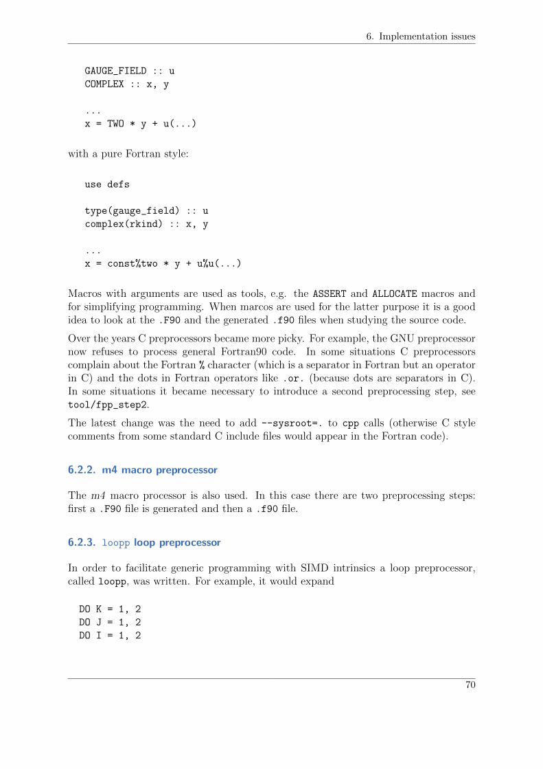
6. Implementation issues
GAUGE_FIELD :: u
COMPLEX :: x, y
...
x = TWO * y + u(...)
with a pure Fortran style:
use defs
type(gauge_field) :: u
complex(rkind) :: x, y
...
x = const%two * y + u%u(...)
Macros with arguments are used as tools, e.g. the ASSERT and ALLOCATE macros andfor simplifying programming. When marcos are used for the latter purpose it is a goodidea to look at the .F90 and the generated .f90 files when studying the source code.
Over the years C preprocessors became more picky. For example, the GNU preprocessornow refuses to process general Fortran90 code. In some situations C preprocessorscomplain about the Fortran % character (which is a separator in Fortran but an operatorin C) and the dots in Fortran operators like .or. (because dots are separators in C).In some situations it became necessary to introduce a second preprocessing step, seetool/fpp_step2.
The latest change was the need to add --sysroot=. to cpp calls (otherwise C stylecomments from some standard C include files would appear in the Fortran code).
6.2.2. m4 macro preprocessor
The m4 macro processor is also used. In this case there are two preprocessing steps:first a .F90 file is generated and then a .f90 file.
6.2.3. loopp loop preprocessor
In order to facilitate generic programming with SIMD intrinsics a loop preprocessor,called loopp, was written. For example, it would expand
DO K = 1, 2
DO J = 1, 2
DO I = 1, 2
70

6. Implementation issues
c%%I%%J = a(I, K) * b(K, J) + c%%I%%J
ENDDO
ENDDO
ENDDO
to:
c11 = a(1, 1) * b(1, 1) + c11
c21 = a(2, 1) * b(1, 1) + c21
c12 = a(1, 1) * b(1, 2) + c12
c22 = a(2, 1) * b(1, 2) + c22
c11 = a(1, 2) * b(2, 1) + c11
c21 = a(2, 2) * b(2, 1) + c21
c12 = a(1, 2) * b(2, 2) + c12
c22 = a(2, 2) * b(2, 2) + c22
6.3. Fortran modules
Modules are used for storing global data, type definitions and a few interface definitions.Global data is always readonly except for its initialisation (there are a few exceptions tothis rule). In general, modules do not contain functions or subroutines. The idea behindthis is that it should always be possible to call functions or subroutines from C/C++ if itshould become necessary to do so. Modules that are only used within the same file areput into that file. Modules that are used by more than one file are put into the modules
subdirectory.
6.4. Precision
Also from the beginning it was foreseen that one might be interested in multi-precisioncode. In principle one can compile any version of BQCD using single precision arithmeticif one defines:
#define RKIND 4
#define BQCD_REAL mpi_real4
This feature was used much later to generate multi-precision code. The recipe is thefollowing.
• The original source file, foo.F90 say, is compiled as usual with double precisionarithmetic.
71

6. Implementation issues
• A single precision version foo_r4.F90 is generated. It contains only four lines:
#define PRECISION_R4
#include "defs.h"
#include "defs_r4.h"
#include "foo.F90"
• defs_r4.h contains macros for renaming all subroutines and functions, e.g.:
#define fun1 fun1_r4
#define fun2 fun2_r4
Again there is also a Fortran way of handling the multi-precision problem. One can useinterfaces and overloading (see su3sc/module_sc.F90).
6.5. Parallelisation
The early versions of BQCD were parallelised by using the shmem library from Cray.Later an MPI version was added and also a single processor version that can be compiledwithout any message passing library. Currently only the MPI and single processorversion work (the routines using shmem are still contained in the distribution). All filesthat use calls to message passing routines are located in directory comm. Which messagepassing library to use can be selected in Makefile.var.
BQCD is parallelised with OpenMP in addition. On the Hitachi SR8000 this lead togreat performance by overlapping communication and computation. In order to facilitateOpenMP programming, BQCD routines contain typically only one loop. It is thenstraightforward to add OpenMP private and reduction declarations: the candidates canbe found in the type declarations of the routine (implicit none is used throughout).
The parallel design is such that results are independent of the numbers of processes used.This is true up to rounding errors introduced by global summations. In a job chain onecan change the number of processes in every job. This feature was implemented, ofcourse, in order to be able to adapt to changing job mixes at computer centres.
6.6. Random numbers
The first random number generator used was ranf by Cray because it has the abilityto jump to an arbitrary position in the sequence of random numbers and this operationis not much more expensive than generating the next random number. This skippingof random numbers was reversely engineered such that it was also available on othercomputers. Skipping is used to generate distributed random numbers in such a way thatresults become independent of the number of processes.
For running production ranlux [36, 37] is the recommended random number generator.In the beginning, the same skipping mechanism as for ranf was used. As a consequence
72
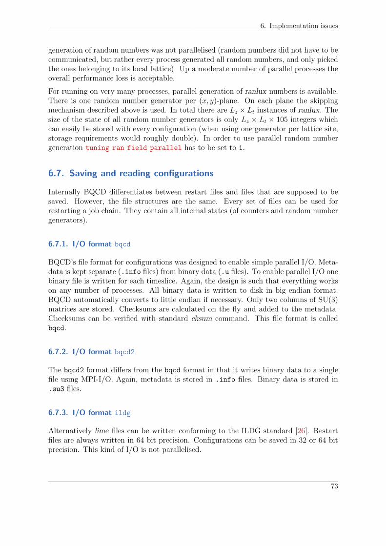
6. Implementation issues
generation of random numbers was not parallelised (random numbers did not have to becommunicated, but rather every process generated all random numbers, and only pickedthe ones belonging to its local lattice). Up a moderate number of parallel processes theoverall performance loss is acceptable.
For running on very many processes, parallel generation of ranlux numbers is available.There is one random number generator per (x, y)-plane. On each plane the skippingmechanism described above is used. In total there are Lz × Lt instances of ranlux. Thesize of the state of all random number generators is only Lz × Lt × 105 integers whichcan easily be stored with every configuration (when using one generator per lattice site,storage requirements would roughly double). In order to use parallel random numbergeneration tuning ran field parallel has to be set to 1.
6.7. Saving and reading configurations
Internally BQCD differentiates between restart files and files that are supposed to besaved. However, the file structures are the same. Every set of files can be used forrestarting a job chain. They contain all internal states (of counters and random numbergenerators).
6.7.1. I/O format bqcd
BQCD’s file format for configurations was designed to enable simple parallel I/O. Meta-data is kept separate (.info files) from binary data (.u files). To enable parallel I/O onebinary file is written for each timeslice. Again, the design is such that everything workson any number of processes. All binary data is written to disk in big endian format.BQCD automatically converts to little endian if necessary. Only two columns of SU(3)matrices are stored. Checksums are calculated on the fly and added to the metadata.Checksums can be verified with standard cksum command. This file format is calledbqcd.
6.7.2. I/O format bqcd2
The bqcd2 format differs from the bqcd format in that it writes binary data to a singlefile using MPI-I/O. Again, metadata is stored in .info files. Binary data is stored in.su3 files.
6.7.3. I/O format ildg
Alternatively lime files can be written conforming to the ILDG standard [26]. Restartfiles are always written in 64 bit precision. Configurations can be saved in 32 or 64 bitprecision. This kind of I/O is not parallelised.
73

6. Implementation issues
6.8. Performance measurements and profiling
A simple profiling mechanism was built in. It can be switched on by defining theTIMING macro. If it is switched off there is no overhead. In the most important routinesoperations were counted manually in order to get performance figures.
6.9. Fermionic boundary conditions
BQCD started with having only one copy of the gauge field. Fermionic boundary condi-tions were imposed by multiplying SU(3) links with -1 accordingly. Flipping boundaryconditions between gluonic and fermionic is handled by subroutine flip_bc(). It hasto be called before and after fermionic operations.
One can optimise the hopping matrix multiplication by introducing a copy of the gaugefield that has an optimised storage ordering. This copy then has fermionic boundaryconditions (and might also include factors 2 from the (1± γ4) projection).
6.10. C interface
C routines have to be called here and there. Examples are checksum calculations, ranluxrandom numbers and I/O of lime files. The Fortran name mangling scheme is selectedby defining NamesToLower, NamesToLOwer_ or NamesToLower__, respectively.
6.11. Input parsing
The input parser checks whether keywords are known but does not check the rest of theline! It is easy to add a new keyword. New keywords can be introduced by adding themto modules/module_input.h. A similar mechanism was used to introduce placeholdersfor ILDG metadata files (see ildg/ildg_meta.F90).
74
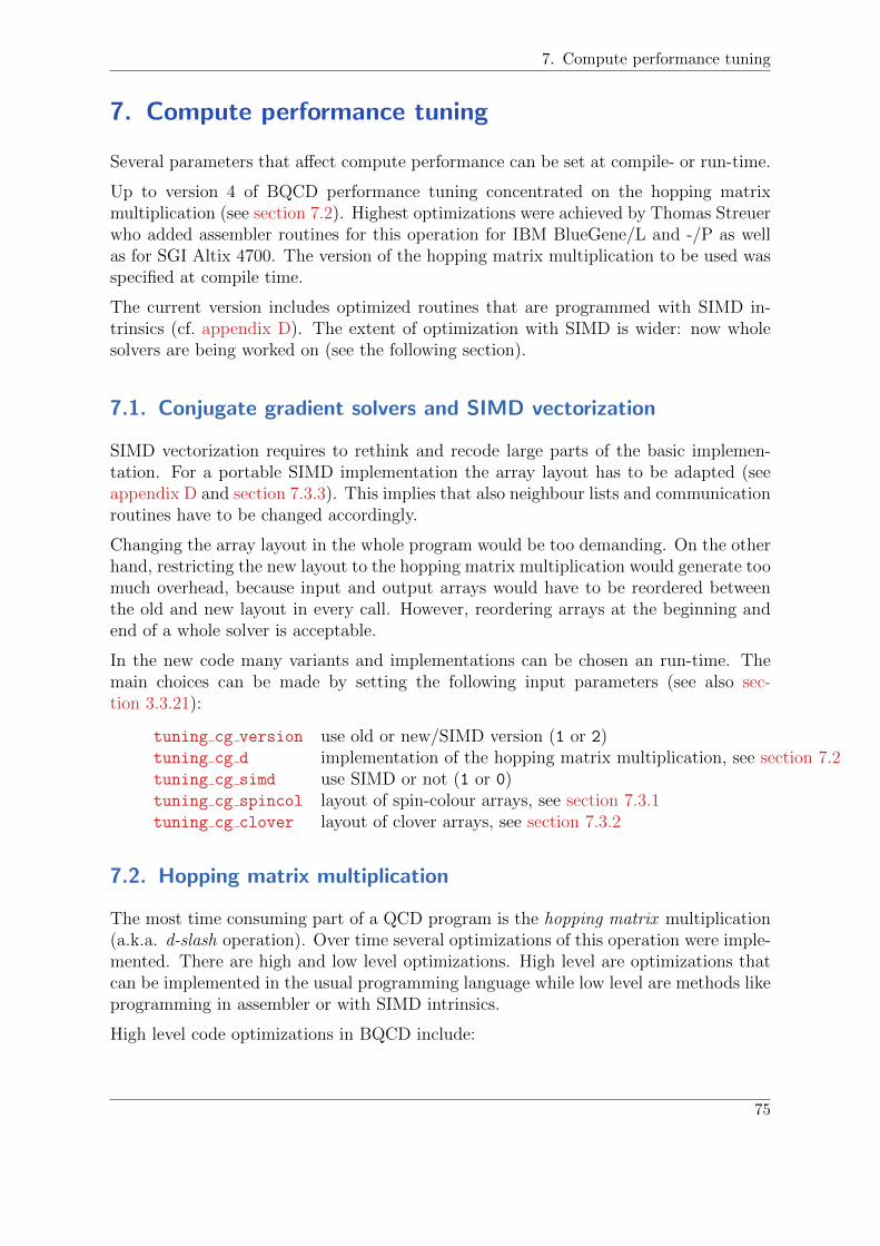
7. Compute performance tuning
7. Compute performance tuning
Several parameters that affect compute performance can be set at compile- or run-time.
Up to version 4 of BQCD performance tuning concentrated on the hopping matrixmultiplication (see section 7.2). Highest optimizations were achieved by Thomas Streuerwho added assembler routines for this operation for IBM BlueGene/L and -/P as wellas for SGI Altix 4700. The version of the hopping matrix multiplication to be used wasspecified at compile time.
The current version includes optimized routines that are programmed with SIMD in-trinsics (cf. appendix D). The extent of optimization with SIMD is wider: now wholesolvers are being worked on (see the following section).
7.1. Conjugate gradient solvers and SIMD vectorization
SIMD vectorization requires to rethink and recode large parts of the basic implemen-tation. For a portable SIMD implementation the array layout has to be adapted (seeappendix D and section 7.3.3). This implies that also neighbour lists and communicationroutines have to be changed accordingly.
Changing the array layout in the whole program would be too demanding. On the otherhand, restricting the new layout to the hopping matrix multiplication would generate toomuch overhead, because input and output arrays would have to be reordered betweenthe old and new layout in every call. However, reordering arrays at the beginning andend of a whole solver is acceptable.
In the new code many variants and implementations can be chosen an run-time. Themain choices can be made by setting the following input parameters (see also sec-tion 3.3.21):
tuning cg version use old or new/SIMD version (1 or 2)tuning cg d implementation of the hopping matrix multiplication, see section 7.2tuning cg simd use SIMD or not (1 or 0)tuning cg spincol layout of spin-colour arrays, see section 7.3.1tuning cg clover layout of clover arrays, see section 7.3.2
7.2. Hopping matrix multiplication
The most time consuming part of a QCD program is the hopping matrix multiplication(a.k.a. d-slash operation). Over time several optimizations of this operation were imple-mented. There are high and low level optimizations. High level are optimizations thatcan be implemented in the usual programming language while low level are methods likeprogramming in assembler or with SIMD intrinsics.
High level code optimizations in BQCD include:
75

7. Compute performance tuning
Loop over directions µ. This is always the outer loop. The inner loop runs over latticesites. In the very first implementation the forward and backward directions ±µwere separate loops. Now the is one inner loop per µ.
Projections (1± γµ)ψ(x∓ µ). Projections reduce 4-component spinors to 2-componentspinors. Projections can be made before or after the exchange of halo regions.One can project at all sites or only at process-boundaries. With our choice ofγ-matrices projection in t-direction involves no computation (it is just a selectionof the upper or lower two spinor components).
Overlapping communication and computation. See section 7.4.2
Version Description Availabilitywith cg version
(see section 7.1)1 2
1 First version (on Cray T3E). There are seven loops: x-forward,x-backward, y-forward, y-backward, z-forward, z-backward, t for-ward and backward
×
2 Four loops (loop fusion of the x, y, z forward/backward loops). × ×21 Version 2 plus reduction of MPI traffic by projecting at all sites
before the halo exchange.× ×
25 Version 2 plus reduction of MPI traffic by projecting only at bound-ary sites sites before the halo exchange (minimal number of pro-jections)
×
3 Version 2 plus overlapping communication and computation. ×35 Version 25 plus overlapping communication and computation. ×100 Version 21 with a customized copy of the gauge field. ×
Table 1: Implementations of the hopping matrix multiplication. The version is specified atcompile time for cg version 1. For cg version 2 it can by chosen at run-time bysetting input parameter tuning cg d.
Descriptions of the implementations of the hopping matrix multiplication are listed intable 1. Version 2 is the fastest implementation in pure OpenMP mode (single pro-cess). Version 3 was the fastest implementation for the Hitachi SR8000, with version 21TFlop/s were sustained on the IBM BlueGene/L and the SGI Altix 4700, and version 100was even a bit faster. Version 25 (single threaded) is the fastest on Cray XC30/40 andversion 35 on IBM BlueGene/Q (3 or 4 symmetric threads per MPI process).
7.3. Array layout
76

7. Compute performance tuning
7.3.1. Spin-colour arrays
There are two layouts for spin-colour arrays that can be used if tuning cg version is2:
• tuning cg spincol = 1
complex(8), dimension (4, 3, volume/2 + boundary)
This layout that is also used in the rest of the program.
• tuning cg spincol = 22
complex(8), dimension (2, 3, volume/2 + boundary, 2)
For the set of γ-matrices that is used in BQCD (see appendix A) this layout leadsto minimal overhead in the exchange of boundary values in t-direction: input andoutput buffers are both consecutive blocks in memory.
7.3.2. Clover arrays
There are two layouts for clover arrays that can be used if tuning cg version is 2:
• tuning cg clover = 1
A packed format (see the source code, file modules/typedef_clover.F90).
This layout that is also used in the rest of the program.
• tuning cg clover = 2
A packed format that is supposed to be better suited for SIMD (see thesource code, file cg/typedef_cg_clover.F90).
Both formats can be used with SIMD and without.
7.3.3. Array layout for SIMD vectorization
If tuning cg simd is 1 the original array layout
complex(8) :: x(dim1, dim2, (volume/2 + boundary), ...)
is changed to
real(8) :: x(B, re:im, dim1, dim2, (volume/2 + boundary) / B, ...)
where B is the SIMD register width (see appendix D).
77

7. Compute performance tuning
7.4. MPI communication
On the first machine that BQCD was running on in production (Cray T3E) it wasadvantageous to exchange boundary values direction by direction. For that machine theboundary exchange was implemented with MPI_Sendrecv.
7.4.1. Overlapping communications
On later and today machines it is advantageous to exchange all boundaries in an over-lapping way. This is implemented with MPI_Irecv, MPI_Isend and MPI_Waitall
do n = 1, n_directions
call mpi_irecv(n)
call mpi_isend(n)
enddo
call mpi_waitall(n_directions)
where the full parameter lists of MPI calls are omitted.
This communication pattern is used by default. It can be switched back to MPI_Sendrecvfor the spin-colour boundary exchange if tuning xbound sc i ist set to 0 and for thegauge field if tuning xbound g i ist set to 0.
7.4.2. Overlapping communication and computation
Overlapping communication and computation is implemented for the boundary exchangeof the spin-colour arrays in the hopping matrix multiplication. The algorithm employedis a two-stage pipeline:
communicate computedirection direction
step 1 y xstep 2 z ystep 3 t zstep 4 t
Technically this is implemented by a hybrid parallelization using MPI plus OpenMP. Themain thread calls MPI while the other threads compute. At least 2 OpenMP-Threadsper MPI process are required.
For cg version 1 overlapping communication and computation is implemented in version 3of the hopping matrix multiplication, for cg version 2 in version 35 of the hopping matrixmultiplication (see table 1).
78

7. Compute performance tuning
7.5. Parallel random numbers
Parallel random number generation is described in section 6.6 (tuning ran field parallel
has to be set to 1).
7.6. I/O
I/O formats are described in section 6.7. Considering performance bqcd is the fastest.bqcd2 is roughly 30 % slower. Both formats use parallel I/O. ildg is not parallel andconsiderably slower. In practice on can use one of the bqcd formats and convert savedconfigurations to the ildg format in a second step by using the --convert-to-ildg
command line option (see section 3.2).
7.7. Miscellaneous
There are several experimental input parameters for further performance tuning, whichare listed here for completeness:
tuning cg precision r4
tuning cg precision
tuning cg loop blocking
tuning cg block length
tuning cg mcg block length
tuning io ildg
79
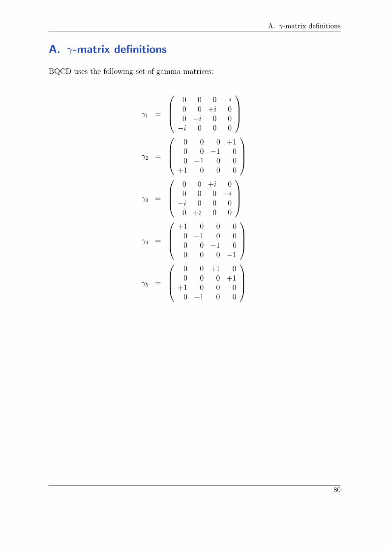
A. γ-matrix definitions
A. γ-matrix definitions
BQCD uses the following set of gamma matrices:
γ1 =
0 0 0 +i0 0 +i 00 −i 0 0−i 0 0 0
γ2 =
0 0 0 +10 0 −1 00 −1 0 0
+1 0 0 0
γ3 =
0 0 +i 00 0 0 −i−i 0 0 0
0 +i 0 0
γ4 =
+1 0 0 0
0 +1 0 00 0 −1 00 0 0 −1
γ5 =
0 0 +1 00 0 0 +1
+1 0 0 00 +1 0 0
80

B. Preprocessor flags – MYFLAGS
B. Preprocessor flags – MYFLAGS
This appendix we list important preprocessor flags that are set via MYFLAGS in Makefile.var
and Makefile.in. Makefile.var has to be adjusted to new platforms while usuallyMakefile.in needs no modification.
B.1. Flags set in Makefile.var
ALIGNMENT VALUE Value in bytes for aligned memory allocation (must fit toUSE_SIMD_* chosen).
CRAY Settings for the Cray compiler.IBM Settings for the IBM compiler.GNU Settings for the GNU compiler.INTEL Settings for the Intel compilerI TIMES MACRO At many places a statement function i times(z) is used.
It returns z multiplied by the imaginary unit. (No floatingpoint operations are necessary here.) Because statementfunctions are outmoded one can achieve the same by usinga preprocessor macro.
LongLong For C source files: 8 byte integers are long long.NamesToLower
NamesToLower
NamesToLower
For C source files: set Fortran name mangling scheme,lower case with no, one or two underscores appended.
OPENMP Is set automatically when compiling C with OpenMP.Needs to be added for preprocessing Fortran (is now addedto FPP rather than MYFLAGS).
TIMING Switch profiling on (time and performance measurement).TRACE Switch on tracing (applies to code in the cg directory).USE MPI WTIME Use MPI Wtime for time measurements.USE SIMD GENERIC
USE SIMD SSE
USE SIMD AVX
USE SIMD AVX2
USE SIMD QPX
Chose SIMD implementation. GENERIC means plain For-tran instead of SIMD intrinsics. ALIGNMENT VALUE has tobe set accordingly.
81

B. Preprocessor flags – MYFLAGS
B.2. Flags set in Makefile.in
DOEDEO If not defined (default) the even/odd ordered hopping ma-trices appear in the preconditioned matrix as DeoDoe andas DoeDeo.
GAMMA NOTATION BQCD γ-matrices are defined according to appendix A.GAMMA NOTATION CHROMA
GAMMA NOTATION CHIRAL
GAMMA NOTATION DDHMC
GAMMAC
Alternative conventions for γ-matrices.
OMTDTD If not defined the preconditioned clover improved fermionmatrix reads
M = Tee −DeoT−1oo Doe and
M = 1− T−1ee DeoT−1oo Doe otherwise.
82

C. Process mapping
C. Process mapping
Process mapping is the mapping of MPI ranks to MPI process coordinates. The func-tionality is similar to Cartesian topologies in MPI.
The following notation is used:
rank MPI rankcoord() process coordinatesprocesses() values of processes, see section 3.3.2process_mapping() values of process mapping, see section 3.3.2
The standard process mapping corresponds to the mapping of the indices of multi-dimensional array to a single index (expressed in Fortran):
rank = 0
rank = rank * processes(4) + coord(4)
rank = rank * processes(3) + coord(3)
rank = rank * processes(2) + coord(2)
rank = rank * processes(1) + coord(1)
Through process mapping the mapping corresponds to a mapping of permutated in-dices:
rank = 0
rank = rank * processes(process_mapping(4)) + coord(process_mapping(4))
rank = rank * processes(process_mapping(3)) + coord(process_mapping(3))
rank = rank * processes(process_mapping(2)) + coord(process_mapping(2))
rank = rank * processes(process_mapping(1)) + coord(process_mapping(1))
83
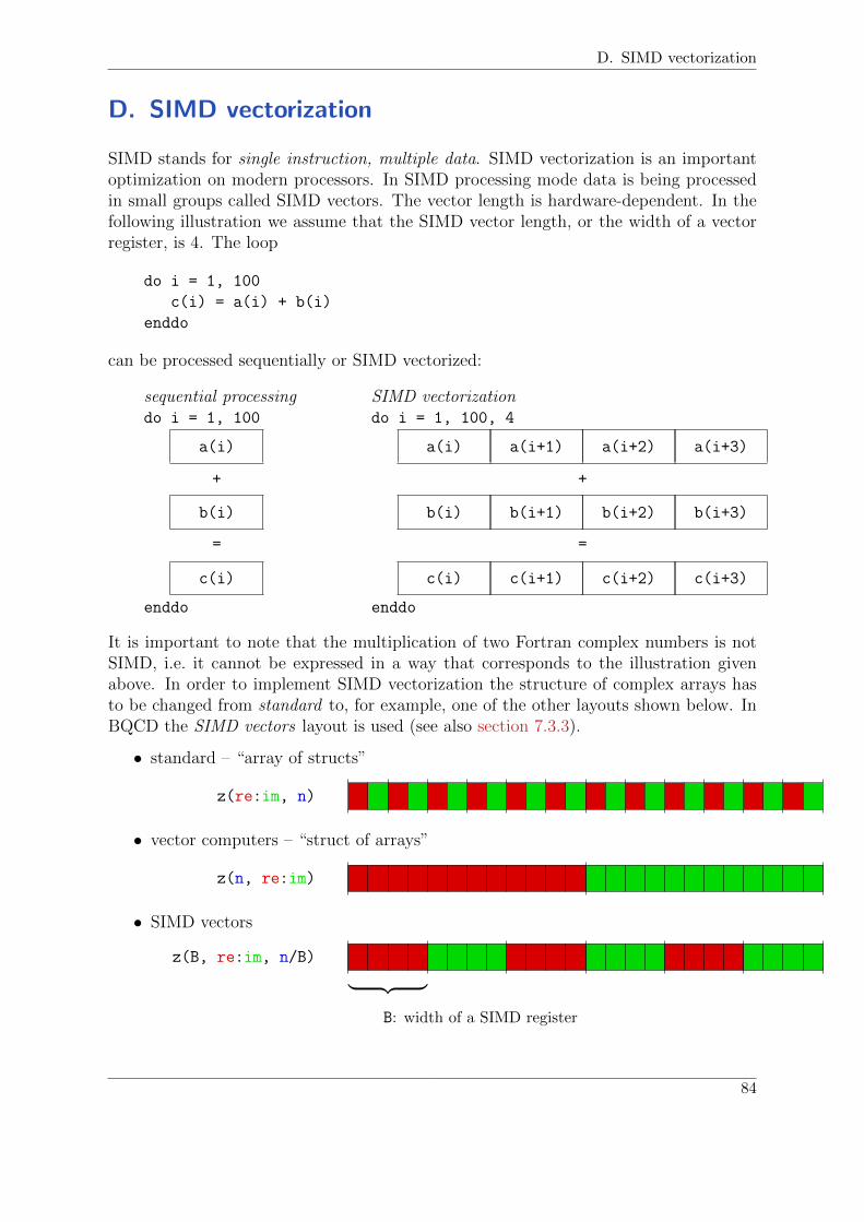
D. SIMD vectorization
D. SIMD vectorization
SIMD stands for single instruction, multiple data. SIMD vectorization is an importantoptimization on modern processors. In SIMD processing mode data is being processedin small groups called SIMD vectors. The vector length is hardware-dependent. In thefollowing illustration we assume that the SIMD vector length, or the width of a vectorregister, is 4. The loop
do i = 1, 100
c(i) = a(i) + b(i)
enddo
can be processed sequentially or SIMD vectorized:
sequential processingdo i = 1, 100
a(i)
b(i)
c(i)
+
=
enddo
SIMD vectorizationdo i = 1, 100, 4
a(i)
b(i)
c(i)
a(i+1)
b(i+1)
c(i+1)
a(i+2)
b(i+2)
c(i+2)
a(i+3)
b(i+3)
c(i+3)
+
=
enddo
It is important to note that the multiplication of two Fortran complex numbers is notSIMD, i.e. it cannot be expressed in a way that corresponds to the illustration givenabove. In order to implement SIMD vectorization the structure of complex arrays hasto be changed from standard to, for example, one of the other layouts shown below. InBQCD the SIMD vectors layout is used (see also section 7.3.3).
• standard – “array of structs”
z(re:im, n)
• vector computers – “struct of arrays”
z(n, re:im)
• SIMD vectors
z(B, re:im, n/B) ︸ ︷︷ ︸B: width of a SIMD register
84
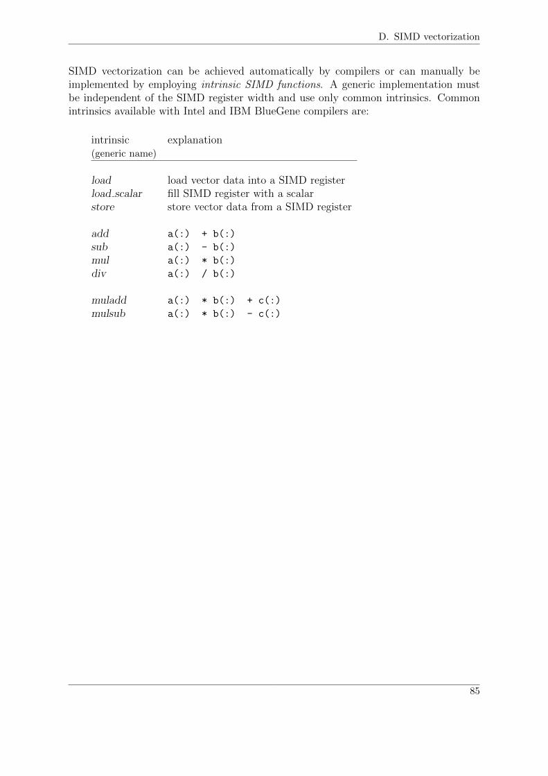
D. SIMD vectorization
SIMD vectorization can be achieved automatically by compilers or can manually beimplemented by employing intrinsic SIMD functions. A generic implementation mustbe independent of the SIMD register width and use only common intrinsics. Commonintrinsics available with Intel and IBM BlueGene compilers are:
intrinsic explanation(generic name)
load load vector data into a SIMD registerload scalar fill SIMD register with a scalarstore store vector data from a SIMD register
add a(:) + b(:)
sub a(:) - b(:)
mul a(:) * b(:)
div a(:) / b(:)
muladd a(:) * b(:) + c(:)
mulsub a(:) * b(:) - c(:)
85

E. Loop blocking
E. Loop blocking
Loop blocking is an optimization technique for loops. For example,
do i0 = 1, n, 256
i1 = min(i0 + (256-1), n)
do i = 1, n do i = i0, i1
a(i) = b(i) + c(i) a(i) = b(i) + c(i)
enddo enddo
−→do i = 1, n do i = i0, i1
x(i) = a(i) * y(i) x(i) = a(i) * y(i)
enddo enddo
enddo
where the block length is 256 and it is assumed that mod(n, 256) == 0. The idea ofthis optimization is to improve data cache locality (i.e. to have a(i) for the second loopin the data cache after blocking).
86

References
References
[1] Y. Nakamura and H. Stuben, PoS(Lattice 2010)040.
[2] T.R. Haar, Y. Nakamura and H. Stuben, Poster presentation at Lattice 2017.
[3] E. M. Ilgenfritz, W. Kerler and H. Stuben, Nucl. Phys. Proc. Suppl. 83 (2000) 831,[arXiv:hep-lat/9908022].
[4] E. M. Ilgenfritz, W. Kerler, M. Muller-Preussker and H. Stuben, Phys. Rev. D 65(2002) 094506 [arXiv:hep-lat/0111038].
[5] H. Stuben [QCDSF-UKQCD Collaboration], Nucl. Phys. Proc. Suppl. 94 (2001)273, [arXiv:hep-lat/0011045].
[6] A. Ali Khan, T. Bakeyev, M. Gockeler, R. Horsley, D. Pleiter, P. Rakow, A. Schafer,G. Schierholz, H. Stuben [QCDSF Collaboration], Phys. Lett. B 564 (2003) 235[arXiv:hep-lat/0303026].
[7] A. Ali Khan, T. Bakeyev, M. Gockeler, R. Horsley, D. Pleiter, P.E.L. Rakow,A. Schafer, G. Schierholz, H. Stuben [QCDSF Collaboration], Nucl. Phys. Proc.Suppl. 129 (2004) 853 [arXiv:hep-lat/0309078].
[8] M. Gockeler et al. [QCDSF Collaboration], PoS LAT2007 (2007) 041[arXiv:0712.3525 [hep-lat]].
[9] N. Cundy et al. [QCDSF-UKQCD Collaborations], PoS LATTICE2008 (2008)132 [arXiv:0811.2355 [hep-lat]].
[10] N. Cundy et al., Phys. Rev. D 79 (2009) 094507 [arXiv:0901.3302 [hep-lat]].
[11] W. Bietenholz et al. [QCDSF-UKQCD Collaborations], PoS LAT2009 (2009) 102[arXiv:0910.2963 [hep-lat]].
[12] X.-Y. Jin, Y. Kuramashi, Y. Nakamura, S. Takeda, A. Ukawa, Phys. Rev. D88(2013) 094508, [arXiv:1307.7205 [hep-lat]] and Phys. Rev. D92 (2015) 114511,[arXiv:1504.00113 [hep-lat]].
[13] A. J. Chambers et al, Phys. Rev. D90 (2014) 014510, [arXiv:1405.3019 [hep-lat]]and Phys. Rev. D92 (2015) 114517, [arXiv:1508.06856 [hep-lat]]
[14] R. Horsley et al., JHEP 1604 (2016) 093, [arXiv:1509.00799 [hep-lat]].
[15] W. Kamleh and M. Peardon Comput. Phys. Comm. 183 (2012) 1993[arXiv:1106.5625 [hep-lat]]
[16] T. Haar, W. Kamleh, J. Zanotti, Y. Nakamura, Comput. Phys. Commun. 215 (2017)113, [arXiv:1609.02652 [hep-lat]].
[17] G. Schierholz and Y. Nakamura, Talk by G.S. at Lattice 2017.
[18] E. M. Ilgenfritz, W. Kerler, M. Muller-Preussker, A. Sternbeck and H. Stuben,Phys. Rev. D 69 (2004) 074511, [arXiv:hep-lat/0309057].
87
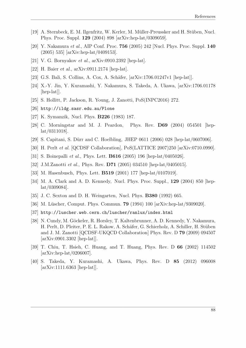
References
[19] A. Sternbeck, E. M. Ilgenfritz, W. Kerler, M. Muller-Preussker and H. Stuben, Nucl.Phys. Proc. Suppl. 129 (2004) 898 [arXiv:hep-lat/0309059].
[20] Y. Nakamura et al., AIP Conf. Proc. 756 (2005) 242 [Nucl. Phys. Proc. Suppl. 140(2005) 535] [arXiv:hep-lat/0409153].
[21] V. G. Bornyakov et al., arXiv:0910.2392 [hep-lat].
[22] H. Baier et al., arXiv:0911.2174 [hep-lat].
[23] G.S. Bali, S. Collins, A. Cox, A. Schafer, [arXiv:1706.01247v1 [hep-lat]].
[24] X.-Y. Jin, Y. Kuramashi, Y. Nakamura, S. Takeda, A. Ukawa, [arXiv:1706.01178[hep-lat]].
[25] S. Hollitt, P. Jackson, R. Young, J. Zanotti, PoS(INPC2016) 272.
[26] http://ildg.sasr.edu.au/Plone
[27] K. Symanzik, Nucl. Phys. B226 (1983) 187.
[28] C. Morningstar and M. J. Peardon, Phys. Rev. D69 (2004) 054501 [hep-lat/0311018].
[29] S. Capitani, S. Durr and C. Hoelbling, JHEP 0611 (2006) 028 [hep-lat/0607006].
[30] H. Perlt et al. [QCDSF Collaboration], PoS(LATTICE 2007)250 [arXiv:0710.0990].
[31] S. Boinepalli et al., Phys. Lett. B616 (2005) 196 [hep-lat/0405026].
[32] J.M.Zanotti et al., Phys. Rev. D71 (2005) 034510 [hep-lat/0405015].
[33] M. Hasenbusch, Phys. Lett. B519 (2001) 177 [hep-lat/0107019].
[34] M. A. Clark and A. D. Kennedy, Nucl. Phys. Proc. Suppl., 129 (2004) 850 [hep-lat/0309084].
[35] J. C. Sexton and D. H. Weingarten, Nucl. Phys. B380 (1992) 665.
[36] M. Luscher, Comput. Phys. Commun. 79 (1994) 100 [arXiv:hep-lat/9309020].
[37] http://luscher.web.cern.ch/luscher/ranlux/index.html
[38] N. Cundy, M. Gockeler, R. Horsley, T. Kaltenbrunner, A. D. Kennedy, Y. Nakamura,H. Perlt, D. Pleiter, P. E. L. Rakow, A. Schafer, G. Schierholz, A. Schiller, H. Stubenand J. M. Zanotti [QCDSF-UKQCD Collaboration] Phys. Rev. D 79 (2009) 094507[arXiv:0901.3302 [hep-lat]].
[39] T. Chiu, T. Hsieh, C. Huang, and T. Huang, Phys. Rev. D 66 (2002) 114502[arXiv:hep-lat/0206007].
[40] S. Takeda, Y. Kuramashi, A. Ukawa, Phys. Rev. D 85 (2012) 096008[arXiv:1111.6363 [hep-lat]].
88