bounds on the sample complexity of bayesian learning using

Machine Learning, 14, 83-113 (1994)© 1994 Kluwer Academic Publishers, Boston. Manufactured in The Netherlands,

Bounds on the Sample Complexity of BayesianLearning Using Information Theory and theVC Dimension

DAVID HAUSSLER [email protected] and Information Sciences, University of California, Santa Cruz, CA 95064

MICHAEL KEARNS [email protected] E. SCHAPIRE [email protected]&T Bell Laboratories, 600 Mountain Avenue, Murray Hill, NJ 07974

Editors: Ming Li and Leslie Valiant

Abstract. In this paper we study a Bayesian or average-case model of concept learning witha twofold goal: to provide more precise characterizations of learning curve (sample complexity)behavior that depend on properties of both the prior distribution over concepts and the sequence ofinstances seen by the learner, and to smoothly unite in a common framework the popular statisticalphysics and VC dimension theories of learning curves. To achieve this, we undertake a systematicinvestigation and comparison of two fundamental quantities in learning and information theory:the probability of an incorrect prediction for an optimal learning algorithm, and the Shannoninformation gain. This study leads to a new understanding of the sample complexity of learningin several existing models.

Keywords: learning curves, VC dimension, Bayesian learning, information theory, average-caselearning, statistical physics

1. Introduction

Consider a simple concept learning model in which the learner attempts to infer anunknown target concept f, chosen from a known concept class f of {0, l}-valuedfunctions over an instance space X. At each trial i, the learner is given a pointxi € X and asked to predict the value of f ( x i ) . If the learner predicts f ( x i )incorrectly, we say the learner makes a mistake. After making its prediction, thelearner is told the correct value.

Informally speaking, there are at least two natural measures of the performanceof a learning algorithm in this setting:

1. The probability the algorithm makes a mistake on f ( x m + 1 ) , having already seenthe examples ( x 1 , f ( x 1 ) ) , . . . , (xm, f ( x m ) ) . Regarded as a function of m, thisfamiliar measure is known as the algorithm's learning curve.

2. The total number of mistakes made by the algorithm on the first m trialsf(x1),...,f(xm). This measure counts the cumulative mistakes of the algo-rithm.

84 D. HAUSSLER, M. KEARNS AND R.E. SCHAPIRE

These measures are clearly closely related to each other. In either measure, we areinterested in the asymptotic behavior of a learning algorithm as m becomes large.Since the learning curve can be used to determine how large m must be before theprobability of mistake drops below a desired value e, the study of learning curvesmay also be viewed as the study of the sample complexity of learning.

The recent and intensive investigation of concept learning undertaken by theresearch communities of neural networks, artificial intelligence, cognitive scienceand computational learning theory has resulted in the development of at leasttwo fairly general and successful viewpoints of the learning process in terms oflearning curves and cumulative mistakes. One of these, arising from the studyof Valiant's distribution-free or probably approximately correct model (1984) andhaving roots in the pattern recognition and minimax decision theory literature,characterizes the distribution-free, worst-case sample complexity of concept learningin terms of a combinatorial parameter known as the Vapnik-Chervonenkis (VC)dimension (Vapnik, 1982; Blumer et al. 1989). In contrast, the average-case samplecomplexity of learning in neural networks has recently been investigated from astandpoint that is essentially Bayesian1, and is strongly influenced by ideas andtools from statistical physics, as well as by information theory (Denker et al., 1987;Tishby, Levin and Solla, 1989; Gyorgyi and Tishby, 1990; Sompolinsky, Tishby andSeung, 1990; Opper and Haussler, 1991). While each of these theories has its owndistinct strengths and drawbacks, there is little understanding of what relationshipshold between them.

In this paper, we study an average-case or Bayesian model of learning with twoprimary goals. First, we are interested in ultimately developing a general frameworkthat provides precise characterizations of learning curves and expected cumulativemistakes that extends and refines the VC dimension and statistical physics theories.The results presented here are a first step in this direction. Second, we wouldlike this framework to smoothly incorporate both of these previous theories, thusyielding a unified viewpoint that can be used both for giving realistic estimates ofaverage-case performance in the case that the distributions on the concept classand instance space are known, and for giving good worst-case estimates in the casethat these distributions are not known.

In a setting where the target concept is drawn at random according to a fixed butarbitrary prior distribution P, we undertake a systematic investigation and compar-ison of two fundamental quantities in learning and information theory: the proba-bility of mistake (known as the 0-1 loss in decision theory) for an optimal learningalgorithm, and the Shannon information gain from the labels of the instance se-quence. In doing so, we borrow from and contribute to the work on weightedmajority and aggregating learning strategies (Littlestone, 1989; Littlestone andWarmuth, 1989; Vovk, 1990; DeSantis, George and Wegman, 1988; Barzdin andFreivald, 1972; Littlestone, Long and Warmuth, 1991), as well as to the VC dimen-sion and statistical physics work. This study leads to a new understanding of thesample complexity of learning in several existing models.

BOUNDS ON THE SAMPLE COMPLEXITY OF BAYESIAN LEARNING 85

One of our main motivations for this research arises from the frequent claims ofmachine learning practitioners that sample complexity bounds derived via the VCdimension are overly pessimistic in practice (Buntine, 1990; Pazzani and Sarrett,1992). This pessimism can be traced to three assumptions that are implicit inresults that are based on the VC dimension. The first pessimistic assumption is thatonly the worst-case performance over possible target concepts counts. This is theminimax pessimism. We may think of an adversary choosing the hardest possibleconcept for the learner, rather than the Bayesian approach which incorporates priorbeliefs regarding which concepts might be "more likely".

The second pessimistic assumption is that even though VC dimension analysisallows a distribution D over the instance space X, this distribution is also assumedto be the hardest possible for learning the class F. Thus, the VC dimension is alsobased on a worst-case assumption over instance space distributions. In additionto the VC dimension, Vapnik and Chervonenkis (1971) have a distribution-specificformulation that overcomes this limitation, but apart from Natarajan's work (1992),it has not been used much in computational learning theory. We extend this ideafurther in Section 9.

The third and perhaps most subtle pessimistic assumption can be seen by not-ing that the VC dimension provides upper bounds on the learning curves of anyconsistent learning algorithm. Thus, even the hypothetical algorithm that alwaysmanages to find a hypothesis that is consistent with the examples so far but thathas the largest possible error with respect to D is covered by VC dimension analy-sis. (This is the uniform convergence property of the VC dimension). In practice itseems unlikely that one would encounter such algorithms — reasonable algorithmsshould manage to find an "average" consistent hypothesis (in terms of error on D)rather than the "worst" consistent hypothesis.

In this paper we attempt to address each of these pessimistic assumptions inthe hopes of obtaining a more realistic picture of sample complexity. To relax theworst-case assumption over the concept class F, we adopt a Bayesian frameworkthat places a prior distribution P over F. If we also assume that the target conceptis drawn according to P, then this allows us to derive bounds on learning curvesand cumulative mistakes that depend on properties of the particular prior P.

Our solution to the worst-case assumption over the instance space distribution Dis twofold. For most of the paper, we in fact do not need to assume that there is adistribution governing the generation of sample points, and instead fix an arbitrarysequence of instances x = x1 , . . . ,xm,xm+1,... that is seen by the learner. Wedo not assume that this sequence is worst-case (distinguishing this setting fromthe various adversary-based on-line learning models that count worst-case mistakebounds), or that it is drawn randomly (distinguishing this setting from the VCdimension and statistical physics theories). Thus our bounds on learning curvesand cumulative mistakes also depend on properties of x. Two advantages thatcome from allowing x to be a parameter are that we incorporate time-dependentinstance sequences, and we model the fact that a learning algorithm does in facthave the training data in its possession, and may be able to exploit this knowledge.


For some of our later results, particularly for comparing our bounds with thosederived via the VC dimension, we will need to revert to the assumption that theinstances in x are generated independently at random according to an instancespace distribution D (but here again, our bounds will depend on properties of theparticular D in contrast to worst-case bounds).

Finally, to address the pessimism implicit in demanding uniform convergence,we will study particular learning algorithms of interest rather than giving boundsfor any consistent algorithm. In addition to analyzing the learning curve and cu-mulative mistakes of the optimal prediction algorithm (the Bayes algorithm), wesimultaneously study the algorithm that outputs a random consistent hypothesis(the Gibbs algorithm). The motivation for this latter algorithm is exactly that ofrelaxing the uniform convergence demand while still making realistic assumptionsabout practical learning algorithms, since this algorithm will output a consistenthypothesis whose error with respect to the instance space distribution D is theaverage (over P), not the worst.

One appealing aspect of our approach is the elementary nature of most of theproofs, which rest almost entirely on well-known or easily derived algebraic expres-sions for the information gain and the probability of mistake, and employ simpleinequalities relating these expressions. The additivity of the Shannon informationis invoked repeatedly in order to obtain easy and useful bounds on otherwise com-plicated sums. For instance, our results include a short and transparent derivationof an upper bound on the expected total number of mistakes in terms of the VCdimension that is tight to within a constant factor.

Perhaps the main strength of this research is the unifying framework it providesfor several previously unrelated theories and results. By beginning in a modelthat averages over both the concept class and the instance space, then graduallyremoving the averaging in favor of combinatorial parameters that upper bound cer-tain expectations, we can move smoothly from the information theoretic bounds ofthe Bayesian and statistical physics theory to bounds based on the VC dimension.Thus, our bounds can be used both for average-case analyses of particular distri-butions, or for worst-case bounds in situations where the prior or instance spacedistribution is arbitrary.

The aim of this paper is to demonstrate the applicability of information theorytools in an average-case learning model, and to show how some important resultsin the VC dimension theory can be reconstructed from these simple mechanisms.Towards ease of exposition and technical simplicity and clarity, we have chosen thesimplest concept learning model that is still of general interest; clearly this modelis far from being a perfect model of the real world. In a later companion paper, wehope to develop our methods further and apply them to more varied and realisticmodels; some of this ongoing work is outlined in Section 12. Many beautiful resultson the performance of Bayesian methods are also given in the statistics literature,see, for example, Clarke and Barron (1990, 1991) and references therein.


2. Summary of results

Following a brief introduction of some notation in Section 3, our results beginin Section 4. Here we define the Shannon information gain of an example, andintroduce the two learning algorithms we shall study. The primary purpose of thissection is to derive expressions for the information gain and the probabilities ofmistake for the two learning algorithms in terms of an important random variableknown as the volume ratio.

In Section 5 we prove that the probabilities of mistake for our two learning al-gorithms can be bounded above and below by simple functions of the expectedinformation gain. As in the paper of Tishby, Levin and Solla (1989), we upperbound the probability of mistake by the information gain. We also provide aninformation-theoretic lower bound on the probability of mistake, which can beviewed as a special case of Fano's inequality (1952; Cover and Thomas, 1991). To-gether these bounds provide a general characterization of learning curve behaviorthat is accurate to within a logarithmic factor.

In Section 6 we exploit the learning curve bounds of Section 5 and the additivityof information to obtain upper and lower bounds on the cumulative mistakes of ouralgorithms that are simple functions of the total information gain. These bounds areagain tight to within a logarithmic factor. The total information gain is naturallyexpressed here as an appropriate entropy expression. This entropy forms the cruciallink between the Bayesian approach and the VC dimension bounds. This link isinvestigated in detail in Section 9.

In Section 7 we investigate the important variation of the basic Bayesian modelin which the target concept / is drawn according to a true prior Q that may differfrom the learner's perceived prior P. We again bound learning curves by informationgain and cumulative mistakes by an entropy depending only on Q plus an additive"penalty term" measuring the distance between P and Q.

In Section 8 we prove that if the instances are chosen randomly according to aninstance space distribution D then the instantaneous information gain is a non-increasing function of m. This result is used in Section 9, where we demonstratethat some important results in the VC dimension theory of learning curves andcumulative mistakes can in fact be recovered from the simple information-theoreticresults in the Bayesian model. This is primarily accomplished by gradually remov-ing averaging over the instance space and the target class in favor of combinatorialparameters that upper bound certain expectations. The main technical tool re-quired is the Sauer/VC combinatorial lemma. In Section 10 we extend these ideasto show how the VC dimension can be used to obtain improved bounds in the casethat the perceived prior and true prior differ.

In Section 12 we draw some conclusions and mention extensions of the resultspresented here.


3. Notational conventions

Before presenting our results, we establish a few notational conventions. Let X bethe instance space. A concept class F over X is a (possibly infinite) collection ofsubsets of X. We will find it convenient to view a concept f e f as a functionf : X — {0,1}, where we interpret f ( x ) = 1 to mean that x e X is a positiveexample of /, and f ( x ) = 0 to mean x is a negative example of /.

The symbols P, Q and D are used to denote probability distributions. Thedistributions P and Q are over F, and D is over X. When F and X are countablewe assume that these distributions are defined as probability mass functions. Foruncountable F and X they are assumed to be probability measures over someappropriate r-algebra. All of our results hold for both countable and uncountableF and X.

We use the notation Efep [X(f)] for the expectation of the random variable xunder the distribution P, and P r f € p [ c o n d ( f ) ] for the probability under the distri-bution V of the set of all / satisfying the predicate cond(f). Everything that needsto be measurable is assumed to be measurable.

4. Instantaneous information gain and mistake probabilities

In this section we begin the analysis of the three quantities that form the backboneof the theory developed here: the Shannon information gain from a labeled exam-ple, and the probability of mistake for the Bayes and Gibbs learning algorithms.Our immediate goal is to define these algorithms and quantities, and to derive ex-pressions for the behavior of each in terms of an important random variable thatwe shall call the volume ratio.

Let F be a concept class over the instance space X. Fix a target concept f € Fand an infinite sequence of instances x = x 1 , . . . , xm, xm + 1 , . . . with xm € X for allm. For now we assume that the fixed instance sequence x is known in advance tothe learner, but that the target concept f is not. Let P be a probability distributionover the concept class F. We think of P in the Bayesian sense as representing theprior beliefs of the learner about which target concept it will be learning.

In our setting, the learner receives information about / incrementally via thelabel sequence f ( x 1 ) , . . . , f(xm), f(xm+1),.... At time m, the learner receives thelabel f(xm). For any m > 1 we define (with respect to x, /) the mth version space

and the mth volume V£(x,f) = P[Fm(x,f)]. We define Fo(x,f) = F for all xand f, so V O ( x , f ) = 1. The version space at time m is simply the class of allconcepts in f consistent with the first m labels of / (with respect to x), and themth volume is the measure of this class under P. For the first part of the paper,the infinite instance sequence x and the prior P are fixed, thus we simply writeFm(f) and V m ( f ) . Later, when we need to discuss distributions other than P, or


when the sequence x is chosen randomly, we will reintroduce these dependenciesexplicitly.

For each m > 0 let us define the mth posterior distribution Pm by restrictingP to the mth version space F m ( f ) , that is, for all (measurable) S c f, Pm[S] =P[Snfm(f)}/P[Fm(f)} = P[Snfm(f)}/Vm(f). Note that Pm has an implicitdependence on x and / that we have omitted for notational brevity. The posteriorprobability distribution Pm can be interpreted as the subjective probability distri-bution over various possible target concepts, given the labels f(x1) , . . . ,f(xm) ofthe first m instances.

Digressing momentarily from the problem of learning /, in this setting we maynow ask the following question: Having already seen f ( x 1 ) , . . . ,f(xm), how muchinformation (assuming the prior P) does the learner gain by seeing f(xm+1)? (Wethink of this as the instantaneous information gain, since we address the gain onlyon the m + 1st label.) The classic answer provided by information theory is thatthe information carried by f ( x m + 1 ) is given by the quantity

where we define the m + 1st volume ratio by

We shall be primarily interested in the expected information gain when / is chosenrandomly according to P, which may now be expressed

We now return to our learning problem, which we define to be that of predictingthe label f (x m + 1 ) given only the previous labels f(x1), . . . , f ( x m ) . The first learn-ing algorithm we consider is called the Bayes optimal classification algorithm (Dudaand Hart, 1973), or the Bayes algorithm for short. It is a special case of the weightedmajority algorithm (Littlestone and Warmuth, 1989). For any m and b € {0,1},define f* (x,f) = f*(f) = {f 6 fm(x,f) : f(xm+1) = b}. Then the Bayesalgorithm behaves as follows:

it predicts that

it predicts that

it flips a fair coin and uses the outcome to predict


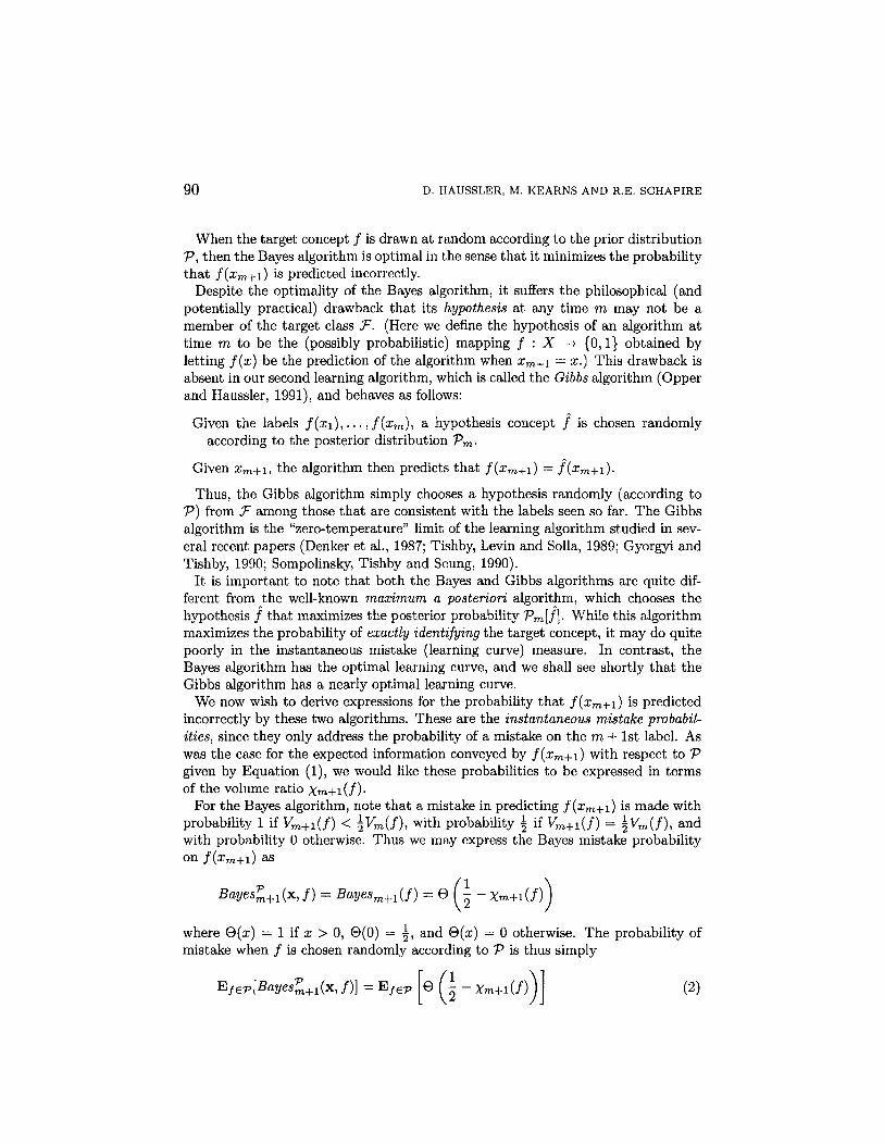
When the target concept / is drawn at random according to the prior distributionP, then the Bayes algorithm is optimal in the sense that it minimizes the probabilitythat f ( x m + 1 ) is predicted incorrectly.

Despite the optimality of the Bayes algorithm, it suffers the philosophical (andpotentially practical) drawback that its hypothesis at any time m may not be amember of the target class F. (Here we define the hypothesis of an algorithm attime m to be the (possibly probabilistic) mapping f : X — {0,1} obtained byletting f ( x ) be the prediction of the algorithm when xm+1 = x.} This drawback isabsent in our second learning algorithm, which is called the Gibbs algorithm (Opperand Haussler, 1991), and behaves as follows:

Given the labels f ( x 1 ) , . . . , f ( x m ) , a hypothesis concept f is chosen randomlyaccording to the posterior distribution Pm.

Given xm+1, the algorithm then predicts that f ( x m + 1 ) = f ( x m + 1 ) .

Thus, the Gibbs algorithm simply chooses a hypothesis randomly (according toP) from F among those that are consistent with the labels seen so far. The Gibbsalgorithm is the "zero-temperature" limit of the learning algorithm studied in sev-eral recent papers (Denker et al., 1987; Tishby, Levin and Solla, 1989; Gyorgyi andTishby, 1990; Sompolinsky, Tishby and Seung, 1990).

It is important to note that both the Bayes and Gibbs algorithms are quite dif-ferent from the well-known maximum a posteriori algorithm, which chooses thehypothesis / that maximizes the posterior probability Pm[f]. While this algorithmmaximizes the probability of exactly identifying the target concept, it may do quitepoorly in the instantaneous mistake (learning curve) measure. In contrast, theBayes algorithm has the optimal learning curve, and we shall see shortly that theGibbs algorithm has a nearly optimal learning curve.

We now wish to derive expressions for the probability that f(xm+1) is predictedincorrectly by these two algorithms. These are the instantaneous mistake probabil-ities, since they only address the probability of a mistake on the m + 1st label. Aswas the case for the expected information conveyed by f(xm+1) with respect to Pgiven by Equation (1), we would like these probabilities to be expressed in termsof the volume ratio X m + 1 ( f ) .

For the Bayes algorithm, note that a mistake in predicting f(xm+1) is made withprobability 1 if V m + 1 ( f ) < \V m ( f ) , with probability i if Vm+1(f) = \Vm(f), andwith probability 0 otherwise. Thus we may express the Bayes mistake probabilityon f(xm+1) as

where @(x) = 1 if x > 0, 9(0) = |, and Q(x) = 0 otherwise. The probability ofmistake when / is chosen randomly according to P is thus simply


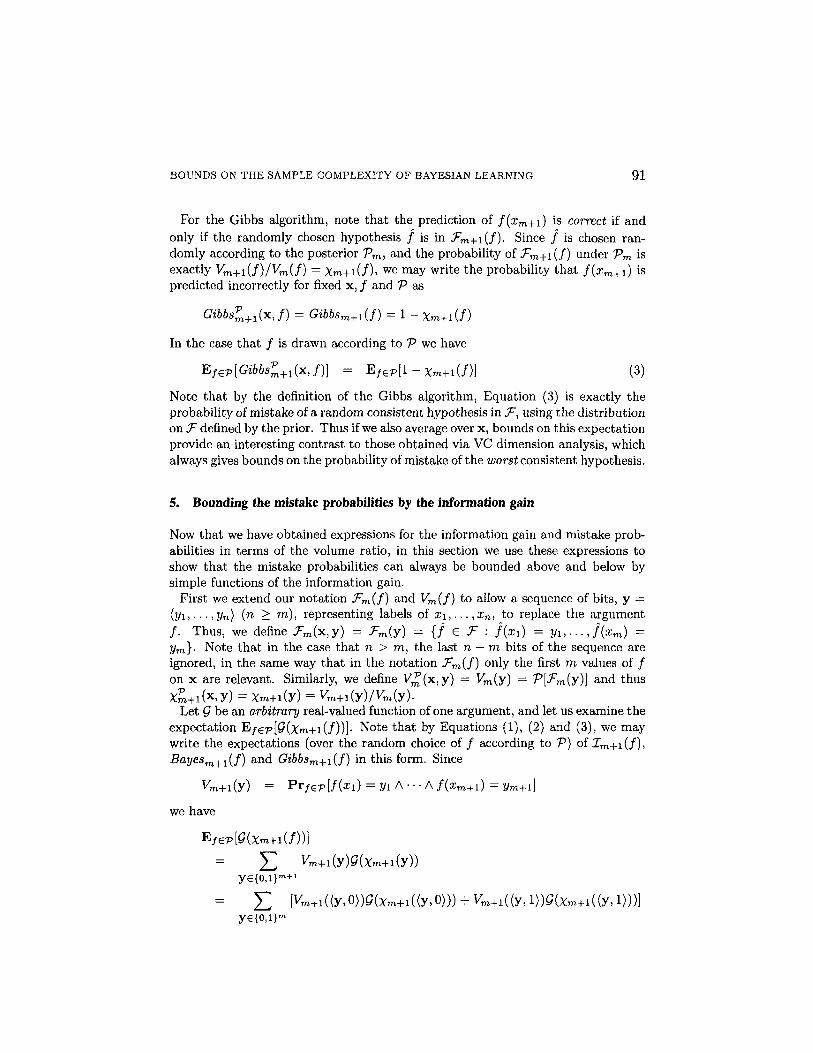
For the Gibbs algorithm, note that the prediction of f(xm+1) is correct if andonly if the randomly chosen hypothesis f is in Fm+1(f). Since f is chosen ran-domly according to the posterior Pm,, and the probability of .Fm+1(f) under Pm isexactly Vm+1(f)/Vm(f) = Xm+1(f), we may write the probability that f(xm+1) ispredicted incorrectly for fixed x, f and P as

In the case that / is drawn according to P we have

Note that by the definition of the Gibbs algorithm, Equation (3) is exactly theprobability of mistake of a random consistent hypothesis in f, using the distributionon F defined by the prior. Thus if we also average over x, bounds on this expectationprovide an interesting contrast to those obtained via VC dimension analysis, whichalways gives bounds on the probability of mistake of the worst consistent hypothesis.

5. Bounding the mistake probabilities by the information gain

Now that we have obtained expressions for the information gain and mistake prob-abilities in terms of the volume ratio, in this section we use these expressions toshow that the mistake probabilities can always be bounded above and below bysimple functions of the information gain.

First we extend our notation F m ( f ) and Vm(f) to allow a sequence of bits, y =( y 1 , . . . , y n ) (n > m), representing labels of x 1 , . . . , x n , to replace the argument/. Thus, we define .Fm(x,y) = -Fm(y) = {f 6 F : f(x1) = y 1 , . . . , f ( x m ) =ym}. Note that in the case that n > m, the last n - m bits of the sequence areignored, in the same way that in the notation Fm(f) only the first m values of /on x are relevant. Similarly, we define V^(x,y) = Vm(y) = P [ F m ( y ) ] and thusXm+1(x,y) = Xm+1(y) = V m + 1 ( y ) / V m ( y ) .

Let G be an arbitrary real-valued function of one argument, and let us examine theexpectation Efep[0(xm+1(f))]- Note that by Equations (1), (2) and (3), we maywrite the expectations (over the random choice of / according to P) of Tm+1(f),B a y e s m + 1 ( f ) and Gibbsm + 1( f ) in this form. Since

we have


where y' is the vector of labels obtained from y by flipping the last label. SinceXm+1(y') = 1 - Xm+1(y), it follows that

The form of the expression inside the expectation of Equation (4) is pQ(p) + (1 —p)G(1 - p) (using the substitution p = Xm+1(f)), and is suggestive of a binary"entropy", in which we interpret p 6 [0,1] as a probability, and Q(p) to be the"information" conveyed by the occurrence of an event whose probability is p.

We now apply Equation (4) to the three forms of Q we have been considering,namely Q(p) = — logp (from Equation (1)), Q(p) = Q(^ — p) (from Equation (2)),and Q(p) = 1 — p (from Equation (3)). From these three equations and some simplealgebra we obtain

for the expected information gain from f ( x m + 1 ) , where H is the familiar binaryentropy function

Note that since 0 < X m + 1 ( f ) < 1> this implies that on average, at most 1 bit ofShannon information can be obtained from a labeled example.

For the probability of mistake of the Bayes algorithm, we obtain

For the probability of mistake of the Gibbs algorithm, we have

Now it is easily verified that for any p € [0,1],


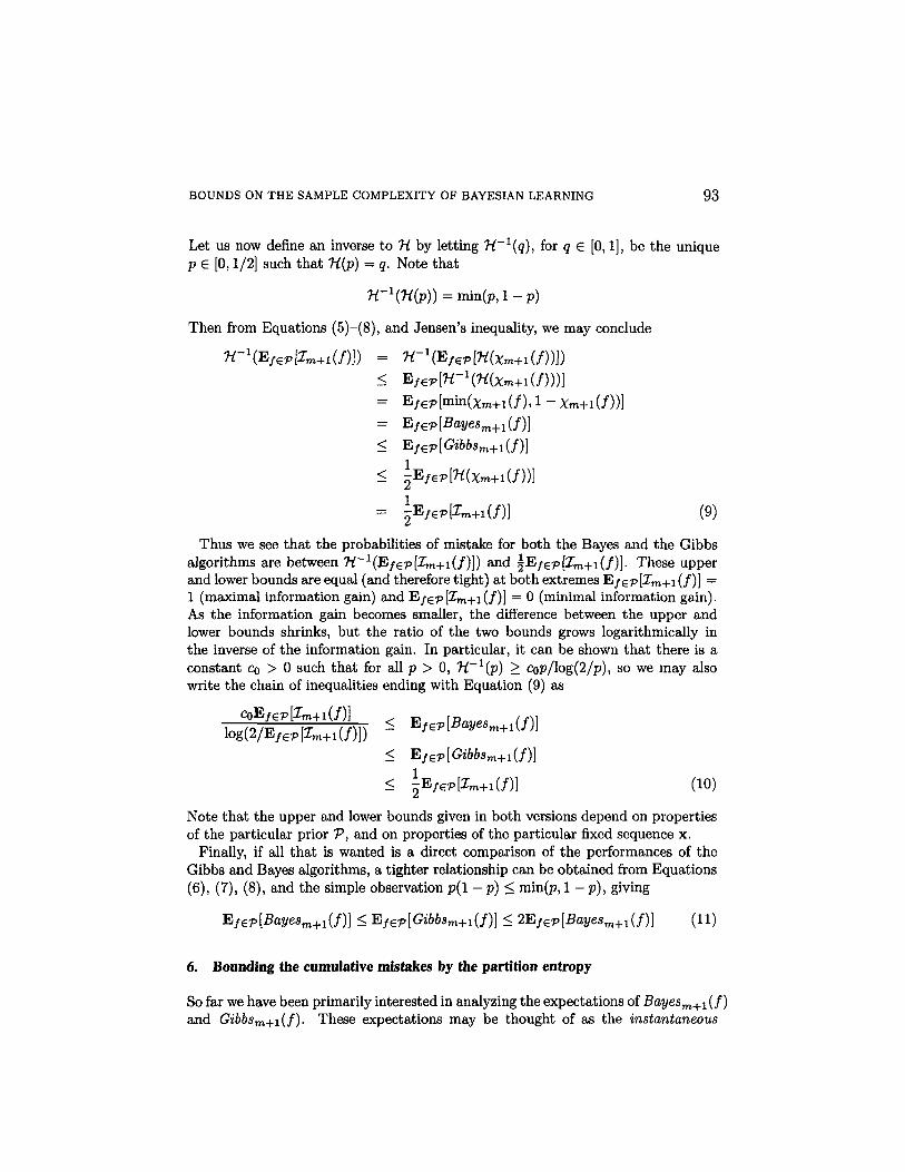
Let us now define an inverse to H by letting H - 1 ( q ) , for q € [0,1], be the uniquep 6 [0,1/2] such that H(p)= q. Note that

Then from Equations (5)-(8), and Jensen's inequality, we may conclude

Thus we see that the probabilities of mistake for both the Bayes and the Gibbsalgorithms are between H-1(Efep[Im+1(f)]) and ^Ef€p[Im+1(f)]. These upperand lower bounds are equal (and therefore tight) at both extremes Efep [Im+1 ( f)] =1 (maximal information gain) and Efep[Zm+1(f)] = 0 (minimal information gain).As the information gain becomes smaller, the difference between the upper andlower bounds shrinks, but the ratio of the two bounds grows logarithmically inthe inverse of the information gain. In particular, it can be shown that there is aconstant C0 > 0 such that for all p > 0, H - l ( p ) > cop/log(2/p), so we may alsowrite the chain of inequalities ending with Equation (9) as

Note that the upper and lower bounds given in both versions depend on propertiesof the particular prior P, and on properties of the particular fixed sequence x.

Finally, if all that is wanted is a direct comparison of the performances of theGibbs and Bayes algorithms, a tighter relationship can be obtained from Equations(6), (7), (8), and the simple observation p(l - p) < min(p, 1 - p), giving

6. Bounding the cumulative mistakes by the partition entropy

So far we have been primarily interested in analyzing the expectations of Bayesm+l (f)and Gibbsm+1(f). These expectations may be thought of as the instantaneous


mistake probabilities: they are the probabilities a mistake is made in predictingf(xm+1), and as such do not explicitly address what happened on the predictionsof f ( x 1 ) , . . . , f(xm). Similarly, Im+1(f) is the instantaneous information, the infor-mation conveyed by f(xm + 1) , without explicit regard for the information conveyedby the previous labels. A natural alternative measure is a cumulative bound —namely, the expected total information gained from the first m labels, or the ex-pected number of mistakes made in the first m trials. While direct analysis of theexpressions for the expected number of mistakes for the Bayes and Gibbs algorithmsis difficult due to the lack of a simple closed-form expression, the situation for thecumulative information gain is quite different due to the additivity of information.More precisely, we may write

since V 0 ( f ) = 1, and recalling the definition of the volume ratio X i ( f ) .The final expression obtained in Equation (12) has a natural interpretation. The

first m instances x1 , . . . ,xm of x induce a partition II^(x) of the concept class Fdefined by Il£(x) = Il£ = {Fm(x,f) : f e F}. Note that |Il£| is always at most2m, but may be considerably smaller, depending on the interaction between f andx1, . . . ,xm. It is clear that

Thus the expected cumulative information gained from the labels of x 1 , . . . ,xm, issimply the entropy of the partition j£ under the distribution P. We shall denotethis entropy by

We may now use this simple expression for the cumulative information gain inconjunction with Jensen's inequality and the chain of inequalities ending with Equa-tion (9) to obtain the following bounds on the expected total number of mistakesmade by the Gibbs and Bayes algorithms on the first m trials:


As in the instantaneous case, the upper and lower bounds here depend on propertiesof the particular P and x. Also, analogous to the instantaneous case, when thecumulative information gain is maximum (W^ = m), the upper and lower boundsare tight, and the ratio of the bounds grows logarithmically as the entropy becomessmall.

These bounds on learning performance in terms of a partition entropy are ofspecial importance to us, since they will form the crucial link between the Bayesiansetting and the Vapnik-Chervonenkis dimension theory.

7. Handling incorrect priors

A common criticism of any Bayesian setting is the assumption of the learner'sknowledge of an accurate prior P. Taken to its logical extreme, this objection leadsus back to worst-case analysis, whose pitfalls and pessimisms we specifically seek toavoid. However, there is a middle ground: namely, we can assume that the learner'sperception of the world (formalized as a perceived prior) may differ somewhat fromthe "truth". In this section we present some initial results in this direction that arebased on the information-theoretic techniques developed thus far.

Let us use Q to denote the true prior and P to denote the perceived prior. Thenwhen / is chosen randomly according to Q but the observer uses the prior P, weobtain the following analogues of Equations (1), (2), and (3):

respectively representing the expected information gain from f ( x m + 1 ) , the proba-bility of mistake for the Bayes algorithm on f (x m + 1 ) , and the probability of mistakefor the Gibbs algorithm on f ( x m + 1 ) .

Since for any 0 < p < 1 we have 0(^ — p) < — logp, it follows that

Since for any 0 < p < 1 we have 1 — p < — lnp = — ln(2) logp, we have


Thus, the probabilities of a mistake on f ( x m + 1 ) for both algorithms are boundedabove by a small constant times the expected information gain. Note that in thisgeneral case in which the prior may be incorrect, the upper bound we get for theGibbs algorithm is actually slightly better than the upper bound we get for theBayes algorithm.

We now obtain bounds on the cumulative number of mistakes on the first m trials.By analogy with Equation (12), from the above we may derive

where W* is the entropy of the partition n^(x) induced on F by x 1 , . . . , xm withrespect to Q, and Im(Q\\P) is the Kullback-Leibler divergence between Q and Pwith respect to this partition.

Our best lower bounds for both the instantaneous mistake probability and thecumulative number of mistakes for the case of an incorrect prior are obtained byobserving that the mistake probability is minimized by the Bayes algorithm whenP = Q. Thus coEfeQ[em+1(f)]/log(2/EfeQ[em+1(f)]) is a lower bound on theinstantaneous mistake probability, and coH%/ log(2m/W^) is a lower bound on thecumulative number of mistakes for both the Bayes and Gibbs algorithms, for anyperceived prior P. It would be interesting to obtain lower bounds that incorporateproperties of the perceived prior P.

8. The average instantaneous information gain is decreasing

In all of our discussion so far, we have assumed that the instance sequence x is fixedin advance, but that the target concept / is drawn randomly according to P. Wenow move to the completely probabilistic model, in which / is drawn according toP, and each instance xm in the sequence x is drawn randomly and independentlyaccording to a distribution D over the instance space X.

In this model, we now prove a result that will be used in the next section, but isalso of independent interest: namely, that the expected instantaneous informationgain Efep,xeD*[Im(x,f)] is a non-increasing function of m. (Here we have intro-duced the notation x e D* to indicate that each element of the infinite sequence xis drawn independently according to D.)


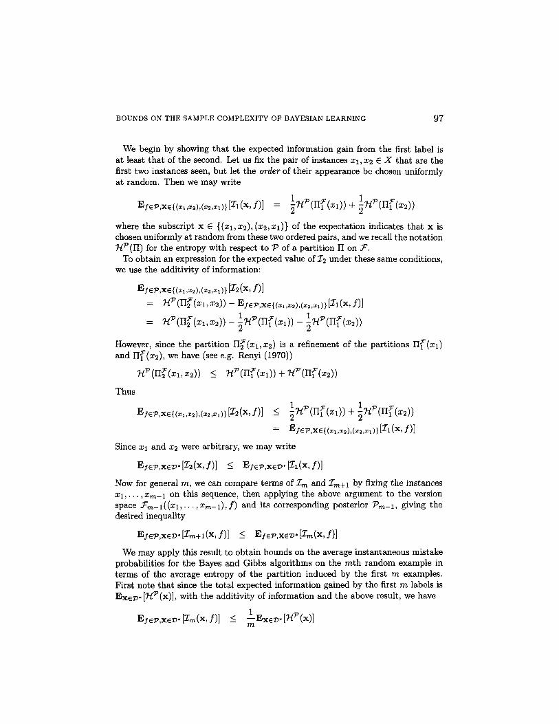
We begin by showing that the expected information gain from the first label isat least that of the second. Let us fix the pair of instances x1, x2 e X that are thefirst two instances seen, but let the order of their appearance be chosen uniformlyat random. Then we may write

where the subscript x £ {(x1, x2), (x2, x1)} of the expectation indicates that x ischosen uniformly at random from these two ordered pairs, and we recall the notationHP(H) for the entropy with respect to P of a partition II on F.

To obtain an expression for the expected value of I2 under these same conditions,we use the additivity of information:

However, since the partition If (x1, x2) is a refinement of the partitions If (x1)and If(x2), we have (see e.g. Renyi (1970))

Thus

Since x1 and x2were arbitrary, we may write

Now for general m, we can compare terms of Im and Jm+1 by fixing the instancesx1,... ,xm-1 on this sequence, then applying the above argument to the versionspace F m - 1 ( ( x 1 , . . . , x m - 1 ) , f ) and its corresponding posterior Pm-1 , giving thedesired inequality

We may apply this result to obtain bounds on the average instantaneous mistakeprobabilities for the Bayes and Gibbs algorithms on the mth random example interms of the average entropy of the partition induced by the first m examples.First note that since the total expected information gained by the first m labels isEXed* [Hp(x)], with the additivity of information and the above result, we have


Thus, using the chain of inequalities ending with Equation (13), we have

For the remainder of the paper we shall find it notationally more convenient todiscuss the instantaneous mistake probability at trial m (as is done in Equation(14)) rather than at trial m + 1.

9. Bayesian learning and the VC dimension: correct priors

Although we have given upper bounds on both the instantaneous probability ofmistake and the expected cumulative number of mistakes for the Bayes and Gibbsalgorithms in terms of Hl (x), we are still left with the problem of evaluating thisentropy, or at least obtaining reasonable upper bounds on it. We can intuitivelysee that the "worst case" for learning occurs when the partition entropy T^(x) isas large as possible. In our context, the entropy is qualitatively maximized whentwo conditions hold:

The instance sequence x induces a partition of f that is the largest possible.

The prior P gives equal weight to each element of this partition.

In this section, we move from our Bayesian average-case setting to obtain worst-casebounds by formalizing these two conditions in terms of combinatorial parametersdepending only on the concept class f. In doing so, we form the link between thetheory developed so far and the VC dimension theory.

The second of the two conditions above is easily quantified. Since the entropy ofa partition is at most the logarithm of the number of classes in it, a trivial upperbound on the entropy which holds for all priors P is

Now let D be a distribution on the instance space X and assume that instances inx are drawn independently at random according to D as in the previous section.Then using Equation (14) we have that for all P,

and using Equation (13) that


The expectation

is the VC entropy defined by Vapnik and Chervonenkis (1971) in their seminalpaper on uniform convergence, and plays a central role in their characterizationof the uniform convergence of empirical frequencies to probabilities in a class ofevents. Here we see how simple information-theoretic arguments can be used torelate the VC entropy to the learning curves of the Bayes and Gibbs algorithms.

In the remainder of this section we will show how the other combinatorial pa-rameter introduced in the paper of Vapnik and Chervonenkis, known in the com-putational learning theory literature as the Vapnik-Chervonenkis (VC) dimensionof the concept class F, can provide useful bounds on the size of I^(x), and howit can be used directly to give bounds on the instantaneous probability of mistakethat are independent of the prior P and the distribution D on the instance spaceX.

We say that the instances x 1 , . . . , xd € X shatter the concept class F if

that is, for every possible labeling of x 1 , . . . , x d there is some target concept inF that gives this labeling. For any set S C X, the Vapnik-Chervonenkis (VC)dimension of F on S, denoted dim(F,S), is the largest d such that there existinstances x1,... ,xd € S that shatter F. If arbitrarily long sequences of instancesfrom S shatter F then dim(F, S) = o. Often 5 = X, so we abbreviate dim(.F, X)by dim(.F). Further, if x = x1, x 2 , . . . is an infinite sequence of instances fromX, for each m > 1 we use dimm(F, x) to denote dim(.F, {x1, ..., xm}). Clearlydimm(F, x) < dim(F) for all x and all m.

The VC dimension has been calculated for many of the fundamental conceptclasses. For example, if the instance space X = ?n and F is the set of all linearthreshold functions on X then dim(F) = n + 1; if the threshold functions arehomogeneous (i.e., the threshold is 0) then dim(F) = n. If f is the set of allindicator functions for axis-parallel rectangles in Jn then dim(F) = 2n; also ifF is the set of all indicator functions for n-fold unions of intervals on X = Rthen dim(F) = 2n. These and many other examples are given in the papers ofDudley (1984) and Blumer et al. (1989) and elsewhere.

The following important combinatorial result relating dimm(F,x) and |n j (x) |has been proven independently by Sauer (1972), Vapnik and Chervonenkis (1982),and others (see Assouad (1983)): for all x,

where o(l) is a quantity that goes to zero as a = m/dimm(F,x) goes to infinity.This result can be used directly in conjunction with Equations (15) and (16) to get


instantaneous and cumulative mistake bounds. Thus we have that for all P,

and

Haussler, Littlestone and Warmuth (1990; Section 3, latter part) show that spe-cific distributions D and priors P can be constructed for each of the classes flisted above (i.e., (homogeneous) linear threshold functions, indicator functions foraxis-parallel rectangles and unions of intervals) for which

This shows that the bound given by Equation (19) is tight to within a factor ofl/ln(2) « 1.44 in each of these cases and hence cannot be improved by more thanthis factor in general. It also follows that the expected total number of mistakes ofthe Bayes and the Gibbs algorithms differ by a factor of at most about 1.44 in eachof these cases; this was not previously known. Opper and Haussler (1991) give asimilar comparison between the instantaneous mistake bounds for the Bayes andGibbs algorithms for homogeneous linear threshold functions using different priorsand instance space distributions. Finally, note that the simplicity of the derivationof the bound in Equation (19) makes this a very appealing way to obtain usefulaverage-case cumulative mistake bounds.

Unfortunately the instantaneous mistake bound given in Equation (18) is notas tight as possible. However, using the results of Haussler, Littlestone and War-muth (1990), we can show that2 for all P,

Ignoring the middle bound for the moment, the proof of this fact is straightfor-ward, given the results of Haussler, Littlestone and Warmuth (1990) (which are


not straightforward to prove, as far as we know). In particular, Theorem 2.3 ofthat paper shows that for any instance space X and any class F of concepts onX, there exists a randomized learning algorithm A (the 1-inclusion graph algo-rithm) such that for any distribution D on X and any target concept f in F, wheninstances x1, ... ,xm are drawn randomly from X according to D and A is given(x 1 , f (x 1 ) ) , • • •, (xm-1,f(xm-1)) and xm, the probability that A makes a mistakepredicting f(xm) is at most dim(F)/m. It follows that for any prior P on f, when/ is selected at random according to P, the probability that A makes a mistakepredicting f(xm) is at most dim(F)/m. Thus the probability of a mistake for Bayesalgorithm is also at most dim(F)/m, by the optimality of Bayes algorithm. (Froma statistical viewpoint, here we are just using the fact that the Bayes risk is alwaysless than the maximum risk of any statistical procedure.)

To prove the middle bound of Equation (21), we can generalize the proof ofHaussler, Littlestone and Warmuth's (1990) Theorem 2.3 to obtain this sharper,instance space distribution dependent form of the bound for the 1-inclusion graphalgorithm for all target concepts, and then apply the argument described in theprevious paragraph to obtain the desired result. Alternately, we can also derive theresult directly from the lemmas used in establishing their Theorem 2.3. This latterapproach is outlined in the discussion section of Haussler (1991).

From Equation (21) we can also obtain similar upper bounds for the Gibbs al-gorithm. In particular, using Equation (11) and Equation (21) we have for allP,

Note that in each of Equations (21) and (22) the second inequality gives a boundthat is independent of the distribution V on the instance space, and of the prior Pon the concept class F.

The same specific distributions and priors constructed by Haussler, Littlestoneand Warmuth (1990) that we mentioned above also show that for each of the classesF of (homogeneous) linear threshold functions, indicator functions for axis-parallelrectangles and unions of intervals, there is an instance space distribution D and aprior P such that

This shows that the bound given by Equation (21) is tight to within a factor of 1/2in each of these cases and hence cannot be improved by more than this factor ingeneral. We conjecture that in fact the lower bound is correct, and thus the upperbounds in Equations (21) and (22) can each be improved by a factor of 1/2. Itshould be noted that if this conjecture holds, then using standard inequalities forpartial sums of the harmonic series, the bounds in Equation (21) could be summedto give bounds similar to those in Equation (19), but using In in place of log.As mentioned above, this bound would be best possible as far as multiplicativeconstants are concerned.


It is both a strength and a weakness of these bounds that they are given in aform that is independent of the prior P, and possibly also of the distribution D onthe instance space: a strength because the same upper bounds hold for all P andV, and a weakness because they may not be tight for specific P and D. While it isalways possible to construct degenerate P and D for which these upper bounds arefar too high, the real question is how far off they are for "typical" or "natural" priorand instance space distributions, as might arise in practice. The distributions usedin the lower bounds from the latter part of Section 3 of Haussler, Littlestone andWarmuth (1990) mentioned above are unfortunately not very natural. However,in a recent paper (Opper and Haussler, 1991) the natural case in which F is theset of homogeneous linear threshold functions on 9d and both the distribution Dand the prior P on possible target concepts (represented also by vectors in £d) areuniform on the unit sphere in Rd is examined. (For homogeneous linear thresholdfunctions only the directions of the target concept and the instance matter, sothe specific choice of the unit sphere is actually immaterial.) In this case, undercertain reasonable assumptions used in statistical mechanics, it is shown that form »d» 1,

(compared with the 0.5d/m conjectured general upper bound and the d/m provengeneral upper bound given for any class of VC dimension d above) and, as waspreviously shown by Gyorgyi and Tishby (1990),

(compared with the 2d/m general upper bound proven above). Thus at least inthis case, the bounds are still accurate to within a constant factor.

10. Bayesian learning and the VC dimension: incorrect priors

We now look at how the notion of VC dimension can be used to get better bounds onthe performance of the Bayes and Gibbs algorithms when the prior P is incorrect —that is, the target concept is actually chosen at random from some different distri-bution Q on F., as in Section 7. Let us say that the prior P is nondegenerate for F iffor any instances x 1 , . . . , xm e X and any f e f, we have V ^ ( ( x 1 , . . . , x m ) , f ) > 0,that is, P never assigns zero probability to any legitimate version space from F.Note that by assigning arbitrarily small probabilities to certain version spaces, theupper bounds given on cumulative mistakes in Section 7 can be made arbitrarilyhigh, even for a nondegenerate prior P. The same holds for the instantaneousmistake bounds. However, the actual probability of mistake, and expected totalnumber of mistakes in m trials, are trivially bounded by 1 and m respectively, sothese bounds cannot be very tight in these extreme cases.

Better-behaved bounds can be obtained using the VC dimension. In particular, interms of instantaneous mistake bounds, it can be shown that for any nondegenerate


prior P, any actual distribution Q on F, and any distribution D on the instancespace

where o(l) represents a quantity that goes to zero as a = m/ dim(F) goes to infinity.A similar result holds for the Bayes algorithm, but with an additional factor of 2,giving

The argument required to establish these bounds is fairly lengthy, and hence isgiven in the appendix.

Because these bounds do not depend on the distribution Q used to choose thetarget concept, they are essentially worst case bounds on the performance of theBayes and Gibbs algorithms over all possible target concepts in F. Furthermore,the bounds in the second inequalities do not depend on the distribution D onthe instance space X either. If tighter versions of these bounds are desired, thedistribution-specific forms given in the middle inequalities may be used.

The middle inequalities also have an interesting consequences when F if finite.In this case we note that |II^m+k(x1,... ,xm+k)| < \F\ for all x1,.. . ,xm+k . Hence

since aln(l + 1/a) < 1 for a > 0, and limQ_0 aln(l + 1/a) = 1. A similar resultholds for the Bayes algorithm with an additional factor of two.

A bound similar to that given in Equation (23) is given by Haussler, Littlestoneand Warmuth (1990), but with a slightly higher constant. As in that paper, itcan be shown that the bound given in Equation (23) holds not only for the Gibbsalgorithm but for any algorithm that always predicts by finding a hypothesis in Fthat is consistent with all the labels of examples it has seen so far (see the appendix).This includes the maximum a posteriori algorithm, which returns the hypothesiswith the maximum posterior probability, mentioned in Section 4. Furthermore,a result given in that paper (Theorem 4.2) shows that the leading asymptoticconstant of 1 in our bound cannot be improved below 1 — 1/e, indicating that for


bounds of this generality, this is about the best that can be done. It is unclearhow information-theoretic tools, or other VC dimension tools such as those usedin obtaining the results of the previous sections, could be used to give strongerversions of this result that depend explicitly on the distributions P and Q.

11. Learning classes of infinite VC dimension

One limitation of the basic VC dimension analysis given thus far is the assumptionthat the target concept is drawn from a class of finite VC dimension. Vapnik hasextended the theory to include the case when F has infinite VC dimension, but canbe decomposed into a sequence f1 C f2 C ... of subclasses with nonzero, finite VCdimensions d 1 , d 2 , . . . , respectively (Vapnik, 1982). A typical decomposition mightlet Fi be all neural networks of a given type with at most i weights, in which casedi = O(ilogi) (Baum and Haussler, 1989).

We can also look at this from a Bayesian point of view by letting the prior P beover all concepts in F, and decomposing it as a linear sum P = Y^=i aiPi, wherePi is an arbitrary prior over Fi and X^i ai = 1. We now derive upper bounds onthe cumulative number of mistakes and the instantaneous mistake probabilities forthe Bayes and Gibbs algorithms by bounding the information gain.

Fix the instance sequence x. As in the analysis of Section 5, we find it convenientto replace the random selection of the target concept f e F with a sequence y e{0, l}m, representing the boolean labels for the first m instances of x. We definePi(y) = Prfept[f(x1) = y1,...,f(xm) = ym]. This immediately gives P(y) =X^i a iP i (y) . Letting H^ denote the entropy with respect to P of the partitioninduced on F by x 1 , . . . , xm (as was done in Section 6), we may write


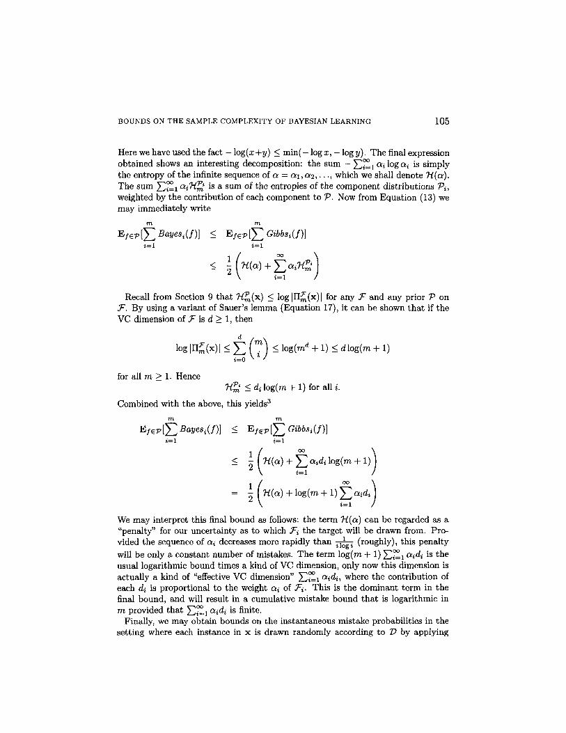
Here we have used the fact - log(x+y) < min(- log x, - log y). The final expressionobtained shows an interesting decomposition: the sum — Y^Liailogai is simplythe entropy of the infinite sequence of a = a1, a2 , . . . , which we shall denote H(a).The sum £^i ai^m is a sum of the entropies of the component distributions Pi ,

weighted by the contribution of each component to P. Now from Equation (13) wemay immediately write

Recall from Section 9 that W^(X)^ log I W(X)I for any F and any prior P onF. By using a variant of Sauer's lemma (Equation 17), it can be shown that if theVC dimension of f is d > 1, then

Combined with the above, this yields3

We may interpret this final bound as follows: the term H(a) can be regarded as a"penalty" for our uncertainty as to which Fi the target will be drawn from. Pro-vided the sequence of ai decreases more rapidly than ^-r (roughly), this penaltywill be only a constant number of mistakes. The term log(m + 1) Y^=i aA is theusual logarithmic bound times a kind of VC dimension, only now this dimension isactually a kind of "effective VC dimension" X^Si ai^i, where the contribution ofeach di is proportional to the weight ai of Fi. This is the dominant term in thefinal bound, and will result in a cumulative mistake bound that is logarithmic inm provided that Y^Li QJ^« is finite.

Finally, we may obtain bounds on the instantaneous mistake probabilities in thesetting where each instance in x is drawn randomly according to D by applying


Equation (14), giving

12. Conclusions and future research

Perhaps the most important general conclusion to be drawn from the work pre-sented here is that the various theories of learning curves based on diverse ideasfrom information theory, statistical physics and the VC dimension are all in factclosely related, and can be naturally and beneficially placed in a common Bayesianframework.

The focus of our ongoing research is that of making the basic theory presented heremore applicable to the situations encountered by practitioners of machine learningin neural networks, artificial intelligence, and other areas. Below we briefly mentionsome extensions of our model for which we have partial results:

Learning with noise. Here we extend many of our general results relying oninformation-theoretic notions to handle the case where the classification labelsmay be corrupted by noise.

Learning multi-valued functions. Here we relax the restriction that the targetfunction have {0, l}-valued output to allow multiple possible output values.These results can be used to study the learning of real-valued functions, whichis often the situation in empirical neural network research.

Learning with other loss functions. In conjunction with the above extension, herewe seek to generalize the theory by studying measures of a learning algorithm'sperformance other than the {0, l}-loss function studied here. A typical choiceis the quadratic loss, often used to obtain the standard sum-of-squared-errorsmeasure for real-valued or vector-valued functions.

Acknowledgements

We are greatly indebted to Manfred Opper and Ron Rivest for their valuable sug-gestions and guidance, and to Sara Solla and Naftali Tishby for insightful ideas inthe early stages of this investigation. We also thank Andrew Barron, Andy Kahn,Nick Littlestone, Phil Long, Terry Sejnowski and Haim Sompolinsky for stimulatingdiscussions on these topics.


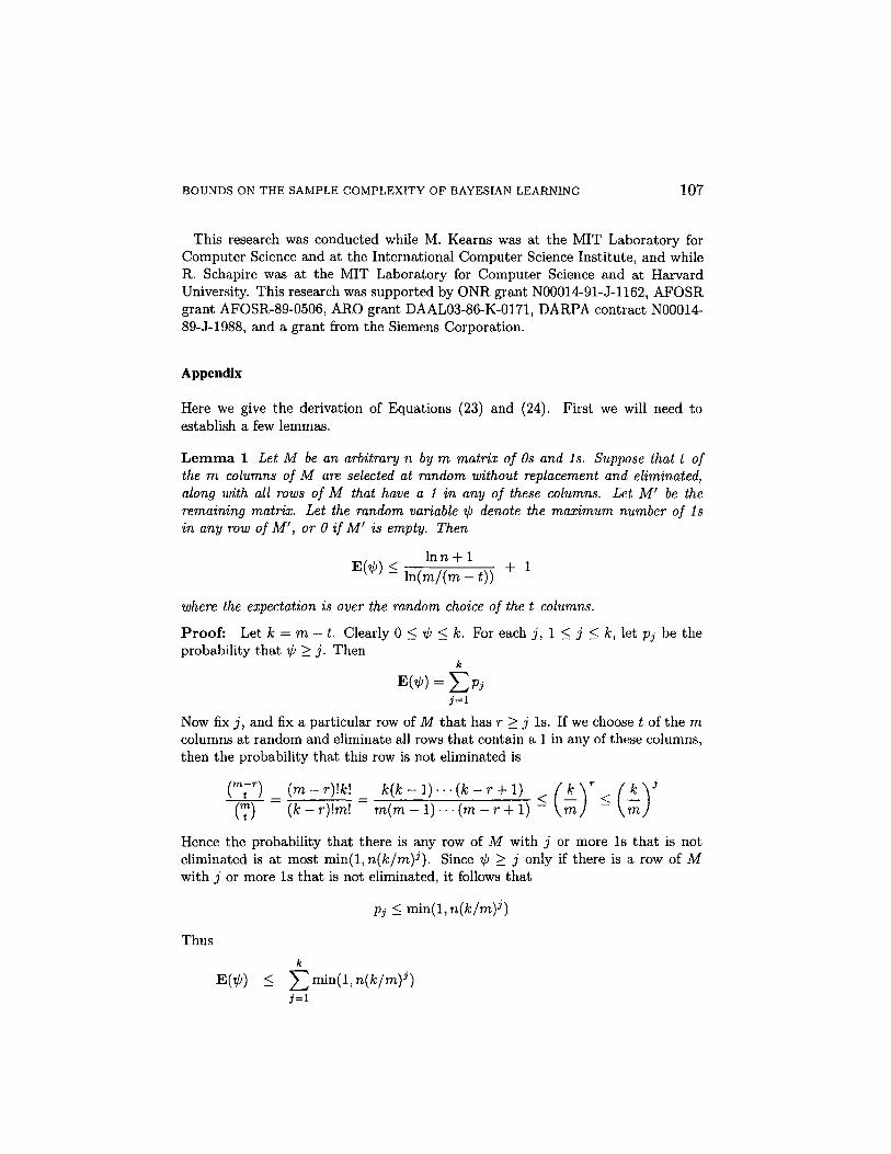
This research was conducted while M. Kearns was at the MIT Laboratory forComputer Science and at the International Computer Science Institute, and whileR. Schapire was at the MIT Laboratory for Computer Science and at HarvardUniversity. This research was supported by ONR grant N00014-91-J-1162, AFOSRgrant AFOSR-89-0506, ARO grant DAAL03-86-K-0171, DARPA contract N00014-89-J-1988, and a grant from the Siemens Corporation.

Appendix

Here we give the derivation of Equations (23) and (24). First we will need toestablish a few lemmas.

Lemma 1 Let M be an arbitrary n by m matrix of 0s and Is. Suppose that t ofthe m columns of M are selected at random without replacement and eliminated,along with all rows of M that have a 1 in any of these columns. Let M' be theremaining matrix. Let the random variable V denote the maximum number of 1sin any row of M', or 0 if M' is empty. Then

where the expectation is over the random choice of the t columns.

Proof: Let k = m - t. Clearly 0 < V < k. For each j, 1 < j < k, let Pj be theprobability that ^ > j. Then

Now fix j, and fix a particular row of M that has r > j Is. If we choose t of the mcolumns at random and eliminate all rows that contain a 1 in any of these columns,then the probability that this row is not eliminated is

Hence the probability that there is any row of M with j or more 1s that is noteliminated is at most min(l,n(k/m) j). Since i > j only if there is a row of Mwith j or more 1s that is not eliminated, it follows that

Thus


Let s be the least integer greater than

Making this substitution and simplifying, we obtain

Since ln(x) < x - 1 for all x > 0, we have

and thus ln((k/(m - k)) ln(m/k)) < 0. It follows that

giving the result. •

Lemma 2 Let P be a nondegenerate prior distribution on f. Let x1 , . . . ,xm beany sequence of instances in the instance space X and f be any (unknown) targetconcept in F. Suppose that t+1 of the m instances x 1 , . . . , xm are selected uniformlyat random without replacement, we are given the values of f on the first t of theseinstances, and we are asked to predict the value of f on the last instance. Then ifwe use the Gibbs learning algorithm with prior P, or indeed any learning algorithmthat always predicts by selecting a hypothesis in F that is consistent with all theexamples it has seen so far, the probability that we predict incorrectly is at most

where n = |II^(x1,..., xm)\. Furthermore, if we use the Bayes algorithm with priorP, the probability that we predict incorrectly is at most twice this value.

Proof: Choose a representative fi e f for each equivalence class of H^(x1 , . . . , xm)for 1 < i < n. Define the n by m matrix M by letting Mi, j = 1 if fi(xj) = f ( x j )and Mi,j = 0 otherwise. Thus each row in M indicates for which instances in


x1 , . . . ,xm the functions in the ith equivalence class will predict the wrong label.In particular, the row representing the equivalence class of / itself is all 0s.

Let us assume that the instances X j 1 , . . . , X j t + 1 are chosen at random withoutreplacement from x1 , . . . ,xm and that we are given the value of / on the firsti of these chosen instances. Consider the problem of predicting the value of /on Xjt+1. Suppose we are using a learning algorithm that predicts by choosing ahypothesis f from F that is consistent with the labels it has seen so far, that is,f ( x j l ) = f (x j l ) , . . . , f ( x j t ) = f ( x j t ) . The Gibbs algorithm is one such algorithm.Since all that matters as far as mistakes in prediction on points in x1 , . . . ,xm

is concerned is the equivalence class of the hypothesis chosen, any such learningalgorithm corresponds to choosing a row i in M with a 0 in each of the t columnsj 1 , . . . , j t . Now since the t + 1st instance x j t+l is randomly chosen from amongthe m — t instances left after the first t instances are chosen, the probability (withrespect to the choice of this t + 1st random instance but fixing the choice of thefirst t instances) that the label of the t + 1st instance is predicted incorrectly isr i / ( m -t), where ri is the number of 1s in the row i of M chosen by the algorithm.

Let M' be the matrix obtained from M by eliminating the t columns j1,.. . , jt,and eliminating any row that has a 1 in any of these columns. Note that M' isnonempty since M has an all 0 row. Then for any row i chosen by a consistentlearning algorithm we have ri/(m — t) < p/(m - t), where V is the maximumnumber of 1s in any row of M'. It follows that the probability (with respect tothe random choice of all t + 1 instances) that the label of this t + 1st instance ispredicted incorrectly is at most E(V)/(m —t), where the expectation is with respectto the random choice of the first t instances. By the previous lemma,

This gives the first result.For the second result, again assume that the instances X j 1 , . . . , Xjt are the first

t instances selected at random (without replacement) from x1 , . . . ,xm and definethe matrix M' as above. Given the labels f(xj1,. . . , f ( x j t ) , let Pt be the posteriordistribution induced on f as defined in Section 4. For each i let Pi denote theprobability, with respect to Pt, of the equivalence class represented by row i of thematrix M'. Since P is nondegenerate, Pi> 0 for each row i of M'.

Let us define the mistake weight p(j) of column j of M' by letting

Thus p(j) is the total posterior probability of all rows that have a 1 in column j.Note that a mistake is made by the Bayes algorithm in predicting the label of thet + lst random instance Xjt+1 with probability 1 if the mistake weight p ( j t+1) > 1/2,and with probability 1/2 if p(jt+i) = 1/2. Thus this probability of a mistake onthe t + 1st random instance is at most 7/(m -t), where 7 is the number of columnsin M' with mistake weight at least 1/2.


Let us define the total mistake weight p of M' by p = ^. p(j). Since the numberof columns with mistake weight at least 1/2 is at most twice the total mistakeweight of all columns, we have 7 < 2p. However, since p = Y^iijPi^ij = 52iPiri,where ri is the number of 1s in row i of M', it is also clear that p < j, where y isthe maximum number of 1s in any row of M'. Hence, the probability of a mistakefor the Bayes algorithm on the t + 1st random instance is at most 2 f / ( m — t). Theremainder of the proof is as above. •

Theorem 1 Let P be a nondegenerate prior on F and Q be any distribution onF. Let D be a distribution on X. Assume the target function f is drawn at randomfrom F according to Q. Suppose that t + 1 instances are selected independently atrandom with replacement from X according to D. Assume we are given the values off on the first t of these instances, and we are asked to predict the value of f on thelast instance. Then if we use the Gibbs learning algorithm, or indeed any learningalgorithm that always predicts by selecting a hypothesis in F that is consistent withall the examples it has seen so far, the probability that we predict incorrectly is atmost

If we use the Bayes algorithm, the probability that we predict incorrectly is at mosttwice this value. Further, if d = dim(F) < o, then this value is at most

where o(l) represents a quantity that goes to zero as t/d goes to infinity.

Proof: Fix k > 1 and let m = t + k. Fix the target concept f e f. The previouslemma shows that for any fixed sequence x = ( x 1 , . . . ,x t + k ) of instances from X,if we randomly select t + 1 of these, and use the labels of the first t to predict thelabel of the t + 1st, then using any consistent learning algorithm, the probabilitywe predict incorrectly is at most

where n = | I£ f e (x) | . Since this bound holds for any fixed sequence x € Xt + k ,it also holds if the Xis in x are drawn independently with replacement from anydistribution on X, when n is replaced with EXeDt+k(|n£j.fc(x)|). However, whenx1,...,xt+k are drawn independently with replacement from some fixed distribu-tion D and then t + 1 of these t + k instances are selected at random (withoutreplacement), the overall distribution on the set of all possible sequences of theresulting t + 1 instances is the same if they were directly selected from D indepen-dently with replacement. Hence, for each k > 1, the value (A.1) above is a boundon the probability of a mistake in predicting the label of the last instance in a se-quence of t + 1, drawn independently with replacement, given the labels of the first


t variables. Finally, since this bound holds for any target f G F, it also holds inexpectation when the target / is selected at random according to any distributionQ on F. This gives the first result of the theorem. The argument is similar for theresult about the Bayes algorithm, using the second part of the previous lemma.

To establish the last result, note that by Sauer's lemma (Equation (17)),

This gives the result. •

Note that the trick employed in the proof above of varying the additional numberof instances k to get better averages has also been used by Shawe-Taylor, Anthonyand Biggs (1989) and by Massart (1986) to get other bounds on related measuresbased on the VC dimension.

Notes

1. More general Bayesian approaches to learning in neural networks are described in recent papers(MacKay, 1992; Buntine and Weigend, 1991).

2. Vapnik (1979) had obtained the special case of this result for homogeneous linear thresholdfunctions. Also, see Talagrand (1988) for further interesting properties of EXED* [dimm(F, x)].

3. Somewhat stronger, but more complex upper bounds can be obtained by using more refinedupper bounds on ^2i=0 (7) •

References

Assouad, P. (1983). Densite et dimension. Annales de l'Institut Fourier, 33(3):233-282.Barzdin, J. M. and Freivald, R. V. (1972). On the prediction of general recursive functions. Soviet

Mathematics-Doklady, 13:1224-1228.Baum, E. and Haussler, D. (1989). What size net gives valid generalization? Neural Computation,

1(1):151-160.


Blumer, A., Ehrenfeucht, A., Haussler, D., and Warmuth, M. K. (1989). Learnability andthe Vapnik-Chervonenkis dimension. Journal of the Association for Computing Machinery,36(4):929-965.

Buntine, W. (1990). A Theory of Learning Classification Rules. PhD thesis, University of Tech-nology, Sydney.

Buntine, W. and Weigend, A. (1991). Bayesian back propagation. Unpublished manuscript.Clarke, B. and Barron, A. (1990). Information-theoretic asymptotics of Bayes methods. IEEE

Transactions on Information Theory, 36(3):453-471.Clarke, B. and Barron, A. (1991). Entropy, risk and the Bayesian central limit theorem, manuscriptCover, T. and Thomas, J. (1991). Elements of Information Theory. Wiley.Denker, J., Schwartz, D., Wittner, B., Solla, S., Howard, R., Jackel, L., and Hopfield, J. (1987).

Automatic learning, rule extraction and generalization. Complex Systems, 1:877-922.DeSantis, A., Markowski, G., and Wegman, M. N. (1988). Learning probabilistic prediction

functions. In Proceedings of the 1988 Workshop on Computational Learning Theory, pages312-328. Morgan Kaufmann.

Duda, R. O. and Hart, P. E. (1973). Pattern Classification and Scene Analysis. Wiley.Dudley, R. M. (1984). A course on empirical processes. Lecture Notes in Mathematics, 1097:2-

142.Fano, R. (1952). Class notes for course 6.574. Technical report, Massachusetts Institute of

Technology.Gyorgyi, G. and Tishby, N. (1990). In Thuemann, K. and Koeberle, R., editors, Neural Networks

and Spin Glasses. World Scientific.Haussler, D. (1991). Sphere packing numbers for subsets of the Boolean n-cube with bounded

Vapnik-Chervonenkis dimension. Technical Report UCSC-CRL-91-41, University of Calif. Com-puter Research Laboratory, Santa Cruz, CA.

Haussler, D., Littlestone, N., and Warmuth, M. (1990). Predicting {0, l}-functions on randomlydrawn points. Technical Report UCSC-CRL-90-54, University of California Santa Cruz, Com-puter Research Laboratory. To appear in Information and Computation.

Littlestone, N. (1989). Mistake Bounds and Logarithmic Linear-threshold Learning Algorithms.PhD thesis, University of California Santa Cruz.

Littlestone, N., Long, P. M., and Warmuth, M. K. (1991). On-line learning of linear functions.In Proceedings of the Twenty Third Annual ACM Symposium on Theory of Computing, pages465-475.

Littlestone, N. and Warmuth, M. (1989). The weighted majority algorithm. Technical ReportUCSC-CRL-89-16, Computer Research Laboratory, University of Santa Cruz.

MacKay, D. (1992). Bayesian Methods for Adaptive Models. PhD thesis, California Institute ofTechnology.

Massart, P. (1986). Rates of convergence in the central limit theorem for empirical processes.Annales de l'Institut Henri Poincare Probabilites et Statistiques, 22:381-423.

Natarajan, B. K. (1992). Probably approximate learning over classes of distributions. SIAMJournal on Computing, 21(3):438-449.

Opper, M. and Haussler, D. (1991). Calculation of the learning curve of Bayes optimal classi-fication algorithm for learning a perceptron with noise. In Proceedings of the Fourth AnnualWorkshop on Computational Learning Theory, pages 75-87. Morgan Kaufmann.

Pazzani, M. J. and Sarrett, W. (1992). A framework for average case analysis of conjunctivelearning algorithms. Machine Learning, 9 (4): 349-372.

Renyi, A. (1970). Probability Theory. North Holland, Amsterdam.Sauer, N. (1972). On the density of families of sets. Journal of Combinatorial Theory (Series A),

13:145-147.Shawe-Taylor, J., Anthony, M., and Biggs, N. (1989). Bounding sample size with the Vapnik-

Chervonenkis dimension. Technical Report CSD-TR-618, University of London, Surrey, Eng-land.

Sompolinsky, H., Tishby, N., and Seung, H. (1990). Learning from examples in large neuralnetworks. Physical Review Letters, 65:1683-1686.

Talagrand, M. (1988). Donsker classes of sets. Probability Theory and Related Fields, 78:169-191.


Tishby, N., Levin, E., and Solla, S. (1989). Consistent inference of probabilities in layered net-works: predictions and generalizations. In IJCNN International Joint Conference on NeuralNetworks, volume II, pages 403-409. IEEE.

Valiant, L. G. (1984). A theory of the learnable. Communications of the ACM, 27(ll):1134-42.Vapnik, V. N. (1979). Theorie der Zeichenerkennung. Akademie-Verlag.Vapnik, V. N. (1982). Estimation of Dependences Based on Empirical Data. Springer-Verlag,

New York.Vapnik, V. N. and Chervonenkis, A. Y. (1971). On the uniform convergence of relative frequencies

of events to their probabilities. Theory of Probability and its Applications, 16(2):264-80.Vovk, V. (1990). Aggregating strategies. In Proceedings of the Third Annual Workshop on

Computational Learning Theory, pages 371-383. Morgan Kaufmann.

bounds on the sample complexity of bayesian learning using

Documents