Boundary­Value Problems in Electrostatics IIReading:  Jackson 3.1 through 3.3,  3.5 through 3.10

Legendre Polynomials

These functions appear in the solution of Laplace's eqn in cases withazimuthal symmetry.

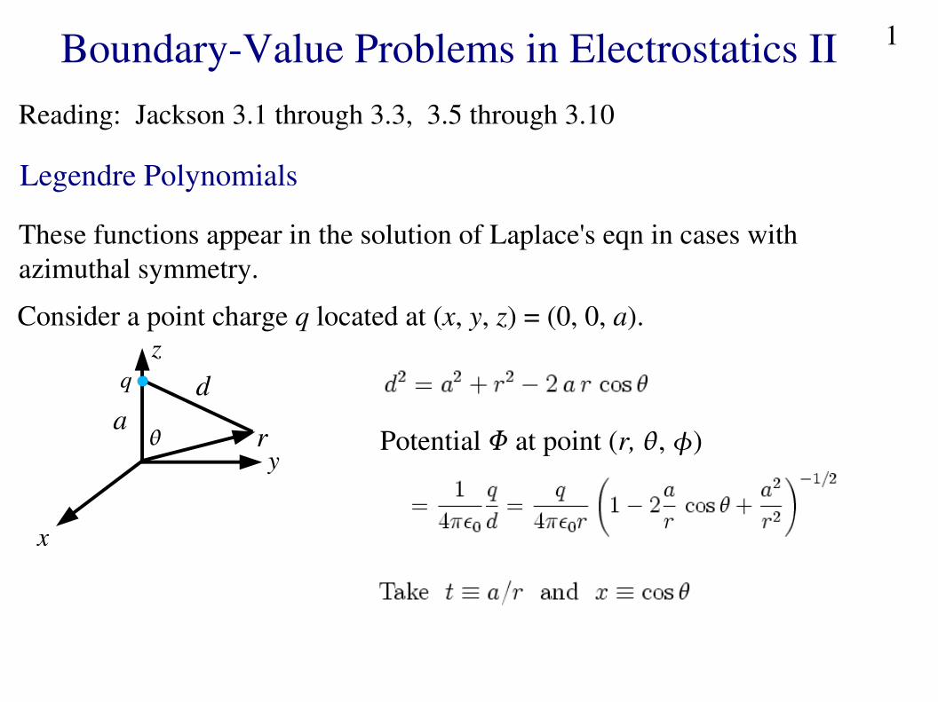
Consider a point charge q located at (x, y, z) = (0, 0, a).

x

y

z

a

d

r Potential  at point (r, , )

1

q

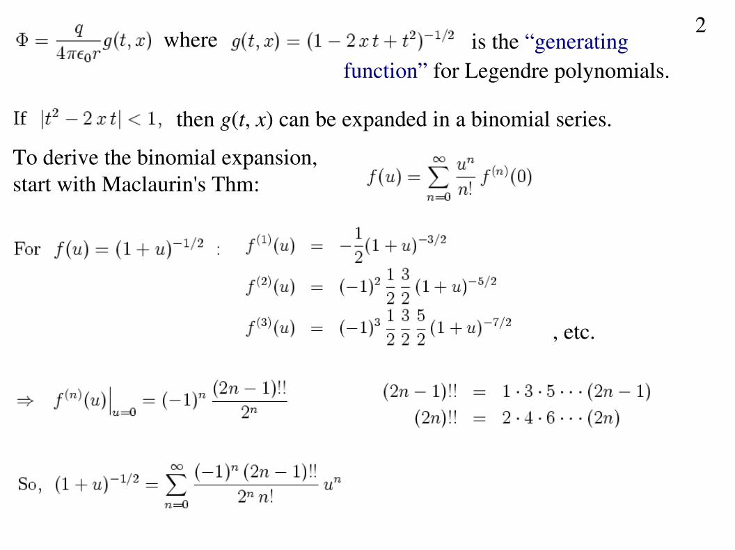
where is the “generating function” for Legendre polynomials.

then g(t, x) can be expanded in a binomial series.

To derive the binomial expansion, start with Maclaurin's Thm:

, etc.

2

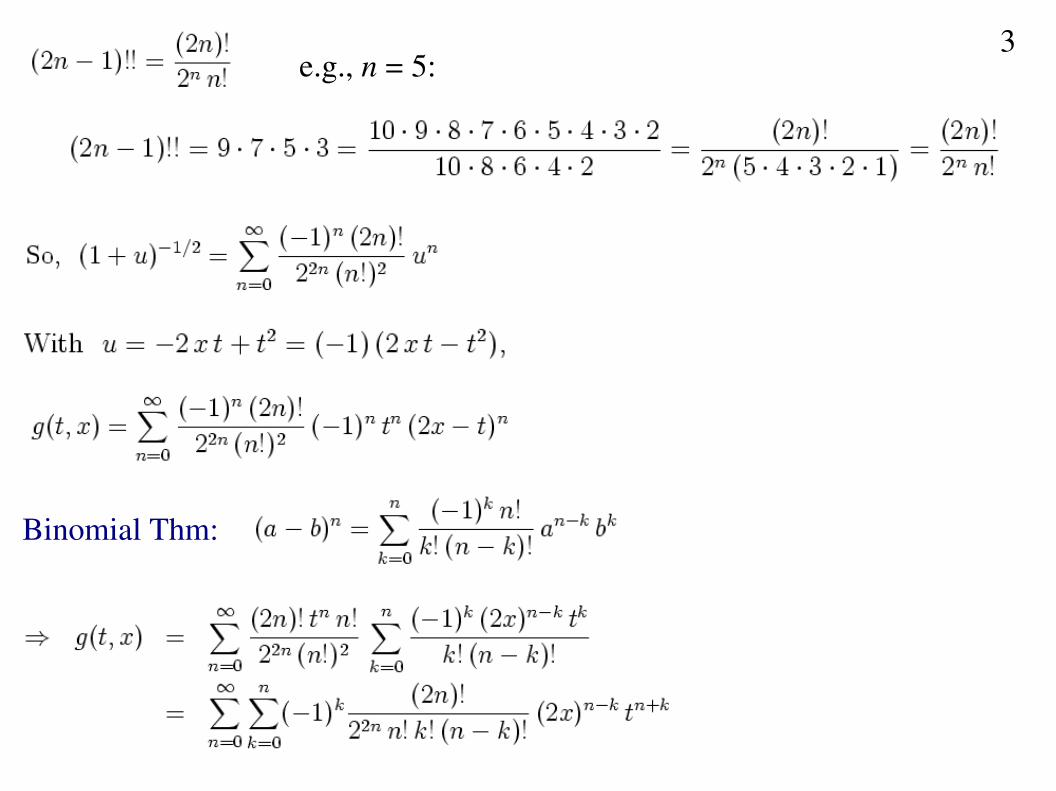
e.g., n = 5:

Binomial Thm:

3

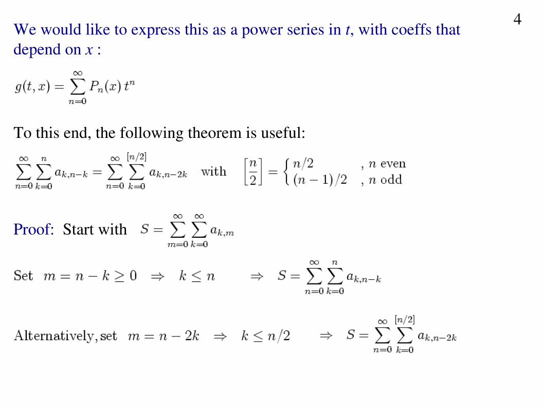
We would like to express this as a power series in t, with coeffs thatdepend on x :

To this end, the following theorem is useful:

Proof:  Start with

4

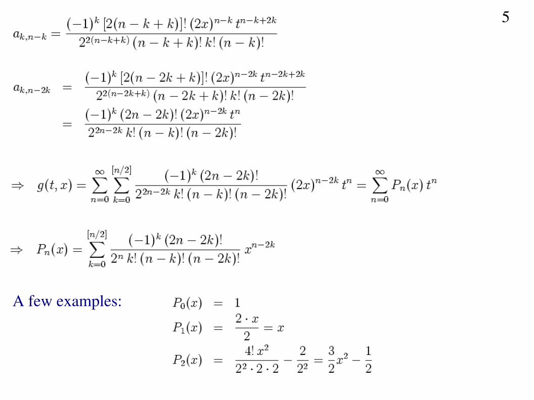
A few examples:

5

=>

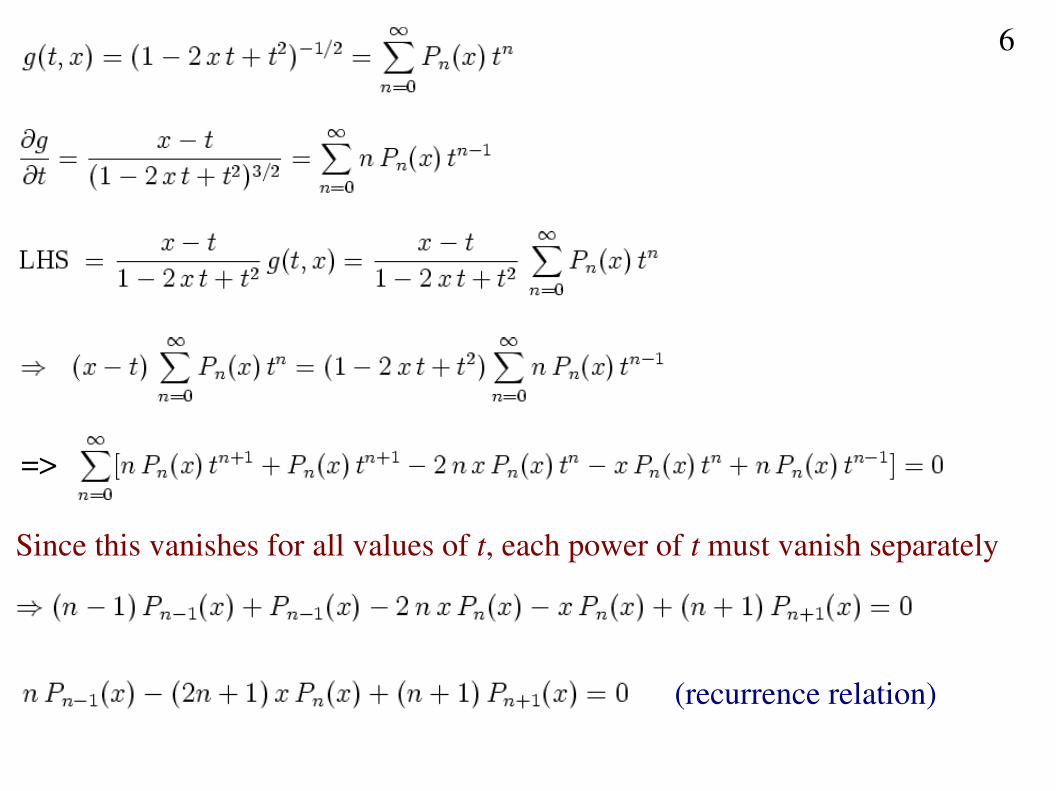
Since this vanishes for all values of t, each power of t must vanish separately  

(recurrence relation)

6

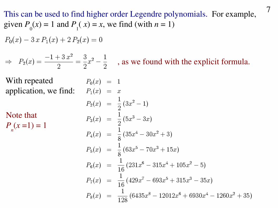
This can be used to find higher order Legendre polynomials.  For example,given P

0(x) = 1 and P

1( x) = x, we find (with n = 1)

, as we found with the explicit formula.

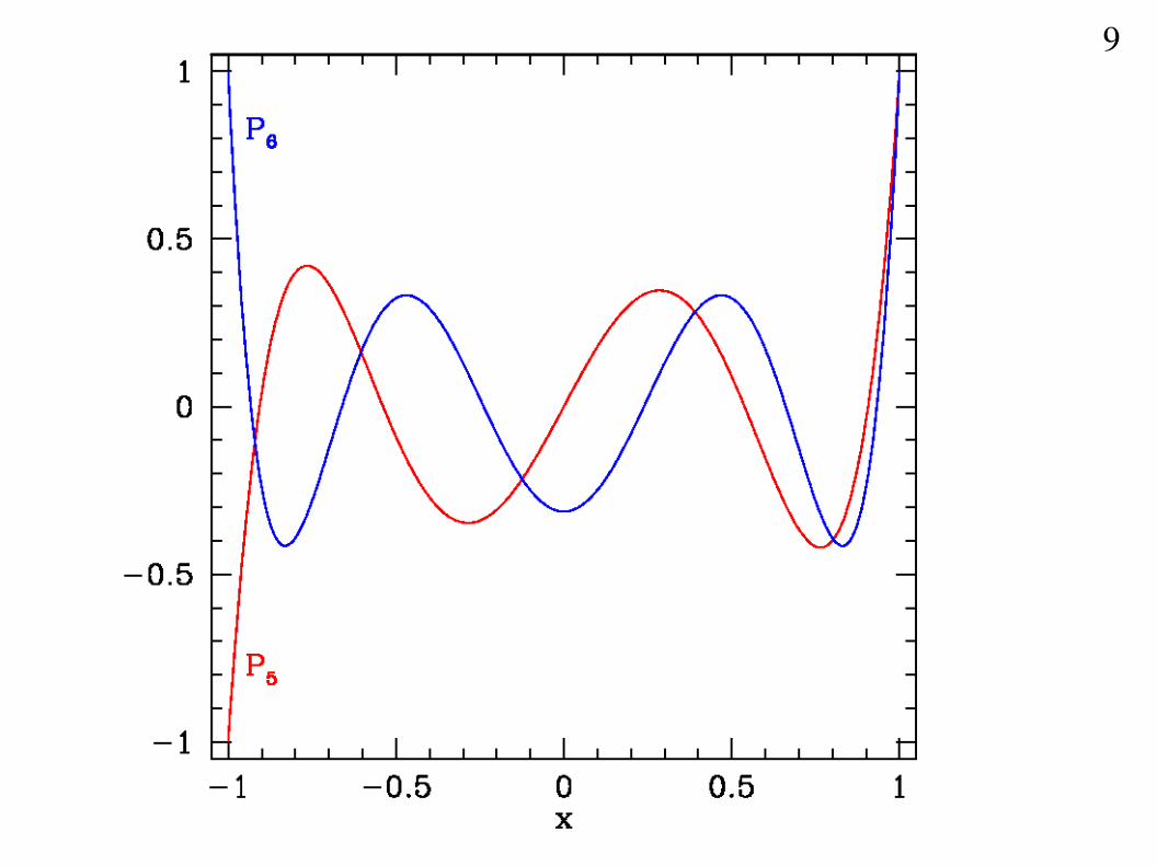
With repeated application, we find:

Note that P

n(x =1) = 1

7

8

9

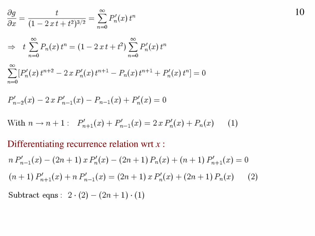
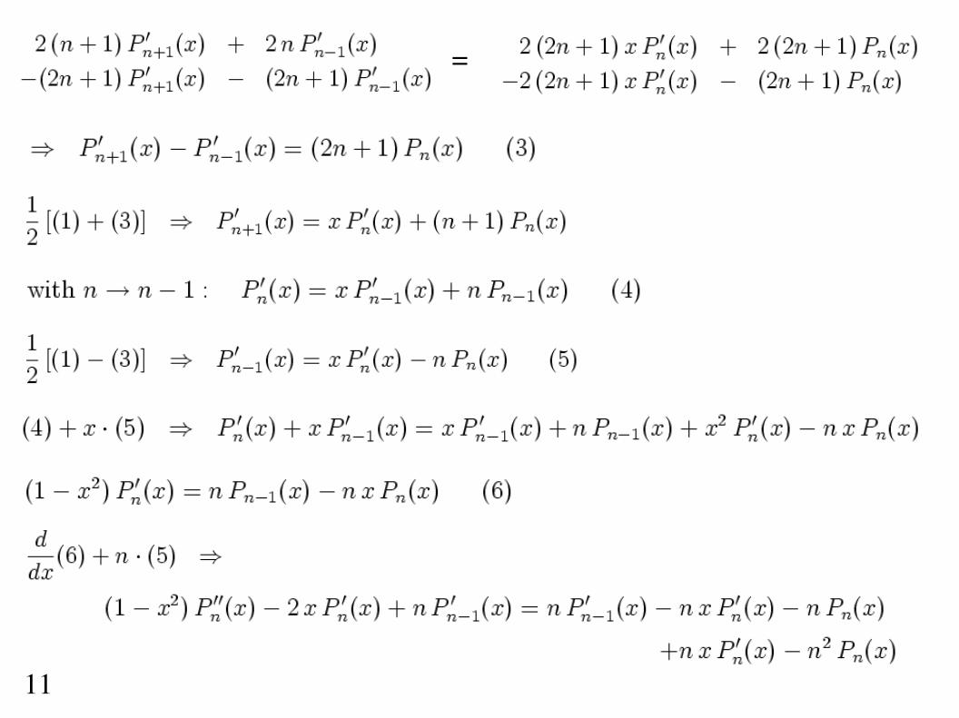
Differentiating recurrence relation wrt x :

10

=

11

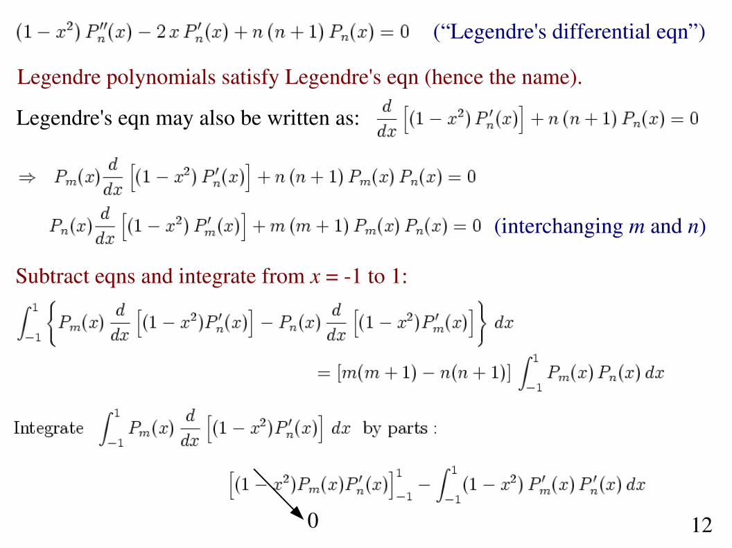
(“Legendre's differential eqn”)

Legendre polynomials satisfy Legendre's eqn (hence the name).

Legendre's eqn may also be written as:

(interchanging m and n)

Subtract eqns and integrate from x = ­1 to 1:

120

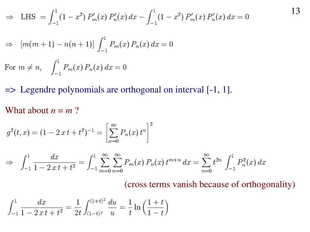
=>  Legendre polynomials are orthogonal on interval [­1, 1].

What about n = m ?

(cross terms vanish because of orthogonality)

13

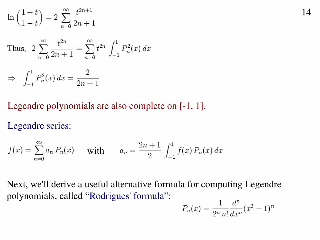
Legendre polynomials are also complete on [­1, 1].

Legendre series:

with

Next, we'll derive a useful alternative formula for computing Legendrepolynomials, called “Rodrigues' formula”:

14

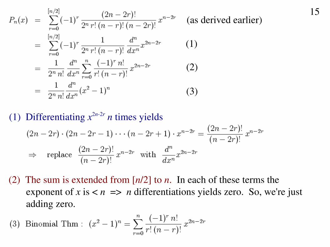
(as derived earlier)

(1)

(2)

(3)

(1)  Differentiating x2n­2r n times yields

(2)  The sum is extended from [n/2] to n.  In each of these terms the       exponent of x is < n  =>  n differentiations yields zero.  So, we're just       adding zero.

15

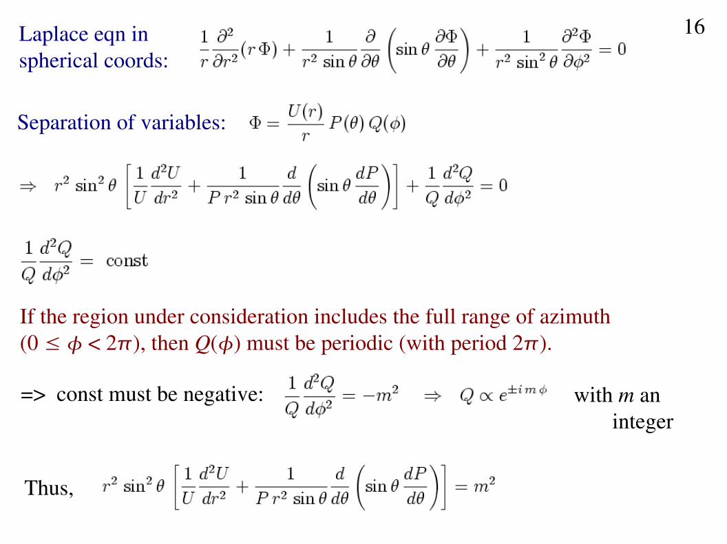
Laplace eqn in spherical coords:

Separation of variables:

If the region under consideration includes the full range of azimuth(0 ≤  < 2), then Q() must be periodic (with period 2).

=>  const must be negative: with m an        integer

Thus, 

16

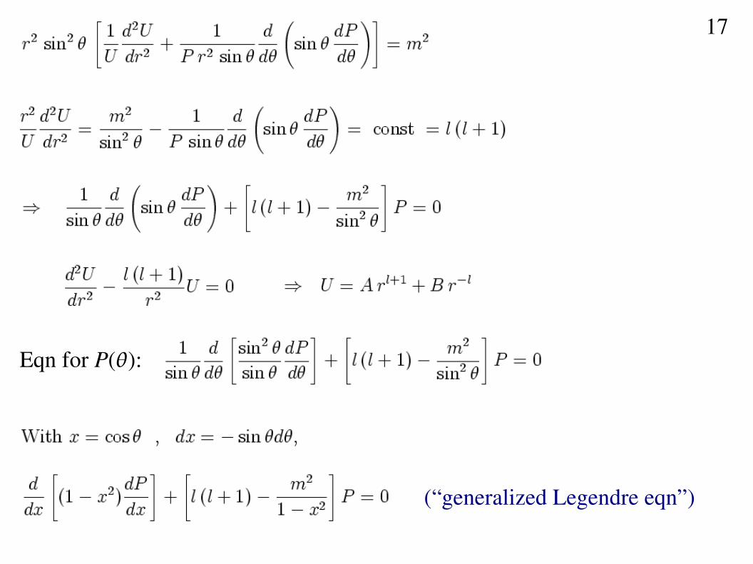
Eqn for P():

(“generalized Legendre eqn”)

17

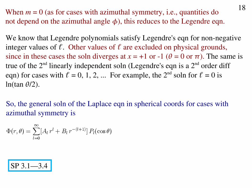
When m = 0 (as for cases with azimuthal symmetry, i.e., quantities do not depend on the azimuthal angle ), this reduces to the Legendre eqn.

We know that Legendre polynomials satisfy Legendre's eqn for non­negativeinteger values of ℓ.  Other values of ℓ are excluded on physical grounds,since in these cases the soln diverges at x = +1 or ­1 ( = 0 or ). The same is true of the 2nd linearly independent soln (Legendre's eqn is a 2nd order diff eqn) for cases with ℓ = 0, 1, 2, ...  For example, the 2nd soln for ℓ = 0 is ln(tan /2).

So, the general soln of the Laplace eqn in spherical coords for cases withazimuthal symmetry is

18

SP 3.1—3.4 

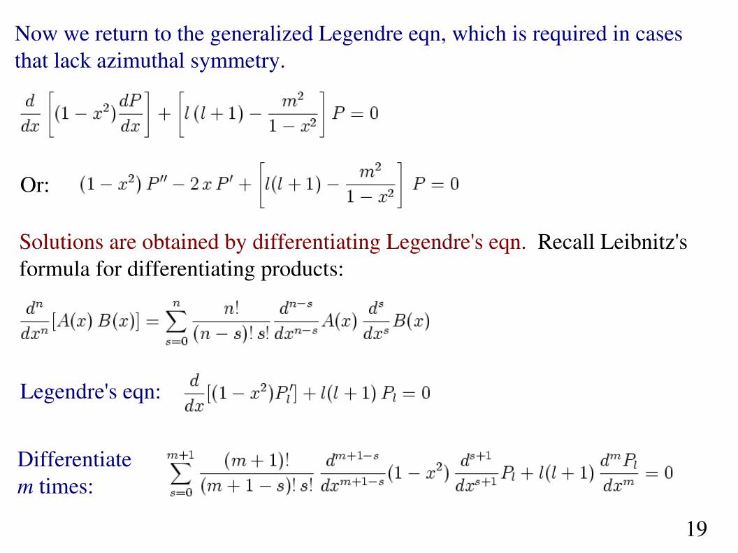
Now we return to the generalized Legendre eqn, which is required in casesthat lack azimuthal symmetry.

Or:

Solutions are obtained by differentiating Legendre's eqn.  Recall Leibnitz'sformula for differentiating products:

Legendre's eqn:

Differentiate m times:

19

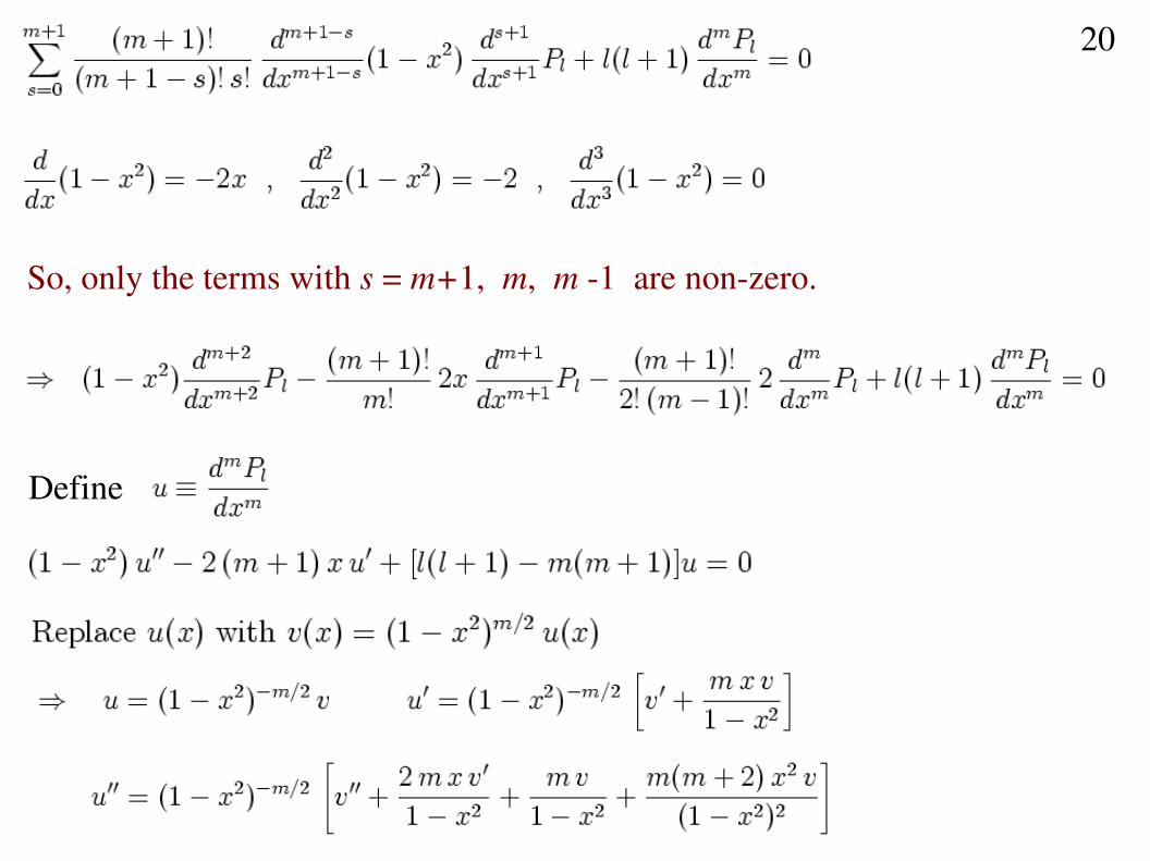
So, only the terms with s = m+1,  m,  m ­1  are non­zero.

Define

20

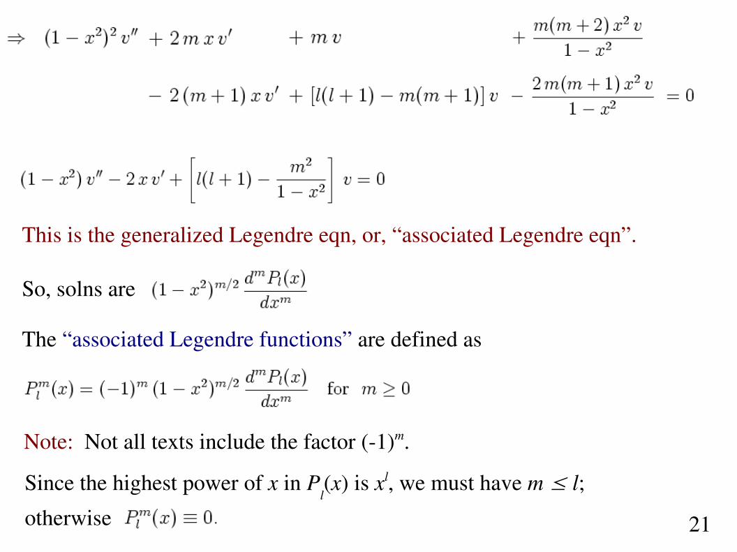
This is the generalized Legendre eqn, or, “associated Legendre eqn”.

So, solns are

The “associated Legendre functions” are defined as

Note:  Not all texts include the factor (­1)m.

Since the highest power of x in Pl(x) is xl, we must have m ≤ l;

otherwise 21

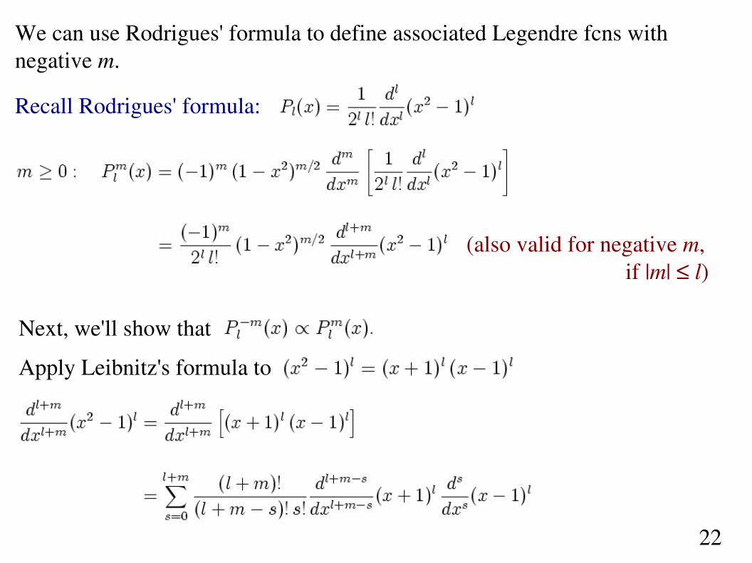
We can use Rodrigues' formula to define associated Legendre fcns withnegative m.

Recall Rodrigues' formula:

(also valid for negative m,                             if |m| ≤ l)

Next, we'll show that

Apply Leibnitz's formula to

22

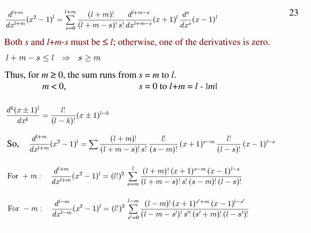
Both s and l+m­s must be ≤ l; otherwise, one of the derivatives is zero.

Thus, for m ≥ 0, the sum runs from s = m to l.                m < 0,                               s = 0 to l+m = l ­ |m|

So,

23

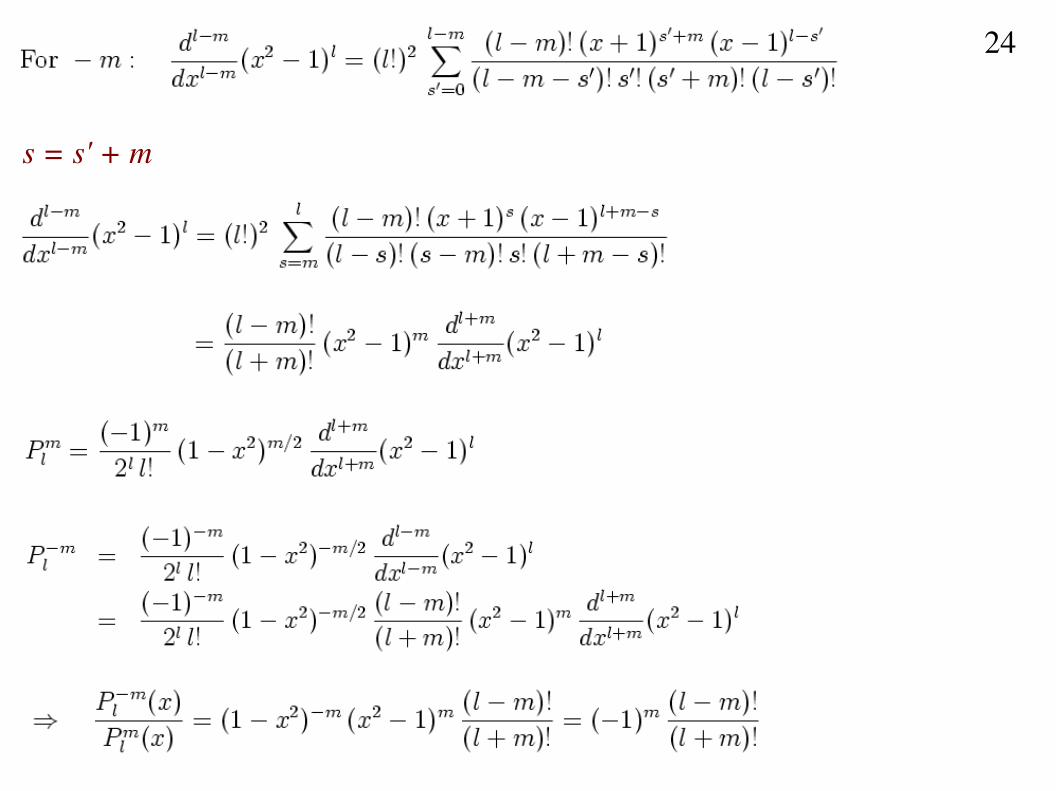
s = s' + m

24

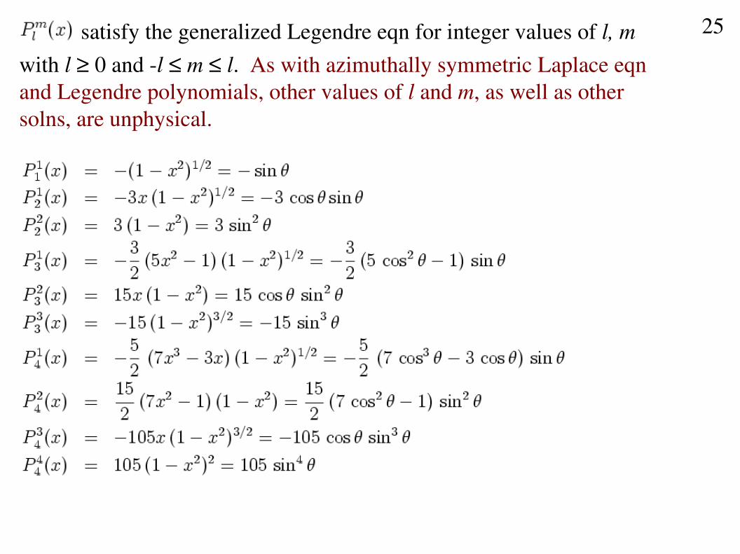
satisfy the generalized Legendre eqn for integer values of l, mwith l ≥ 0 and ­l ≤ m ≤ l.  As with azimuthally symmetric Laplace eqn and Legendre polynomials, other values of l and m, as well as othersolns, are unphysical.

25

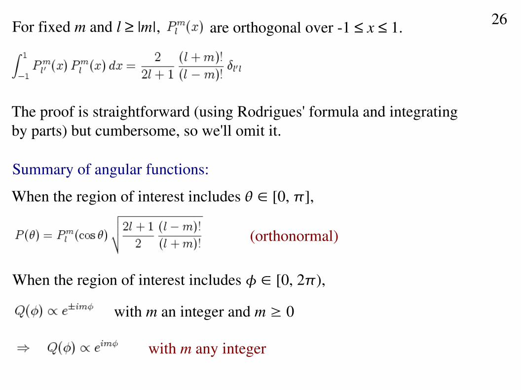
For fixed m and l ≥ |m|, are orthogonal over ­1 ≤ x ≤ 1.

The proof is straightforward (using Rodrigues' formula and integratingby parts) but cumbersome, so we'll omit it.

Summary of angular functions:

When the region of interest includes  ∈ [0, ],

(orthonormal)

When the region of interest includes  ∈ [0, 2),

with m an integer and m ≥ 0

with m any integer

26

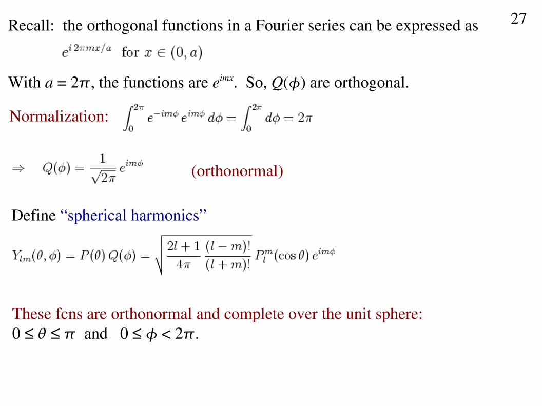
Recall:  the orthogonal functions in a Fourier series can be expressed as

With a = 2, the functions are eimx.  So, Q() are orthogonal.

Normalization:

(orthonormal)

Define “spherical harmonics”

These fcns are orthonormal and complete over the unit sphere:0 ≤  ≤   and   0 ≤  < 2.

27

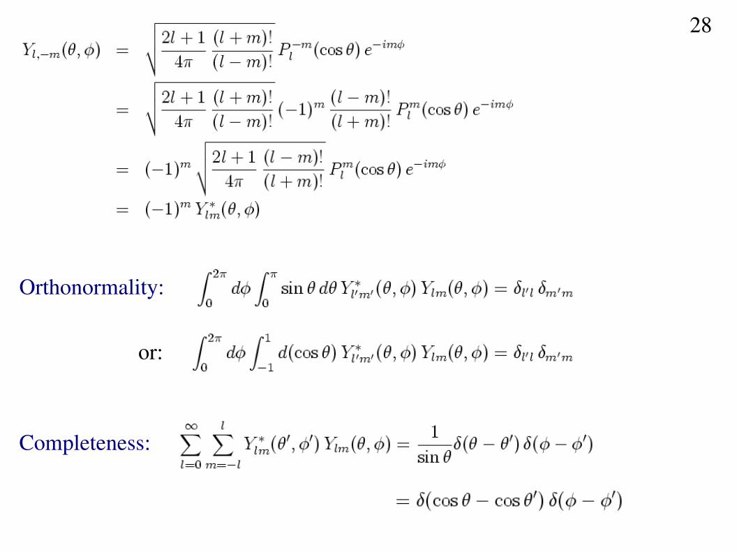
Orthonormality:

or:

Completeness:

28

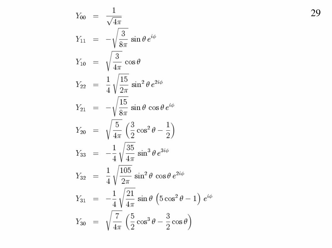
29

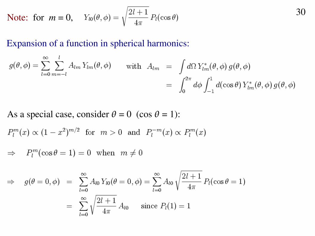
Note:  for  m = 0,

Expansion of a function in spherical harmonics:

As a special case, consider  = 0  (cos  = 1):

30

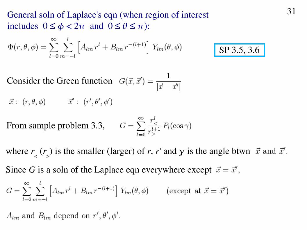
General soln of Laplace's eqn (when region of interest includes  0 ≤  < 2  and  0 ≤  ≤ ):

Consider the Green function

From sample problem 3.3,

where r< (r

>) is the smaller (larger) of r, r' and  is the angle btwn 

Since G is a soln of the Laplace eqn everywhere except

31

SP 3.5, 3.6

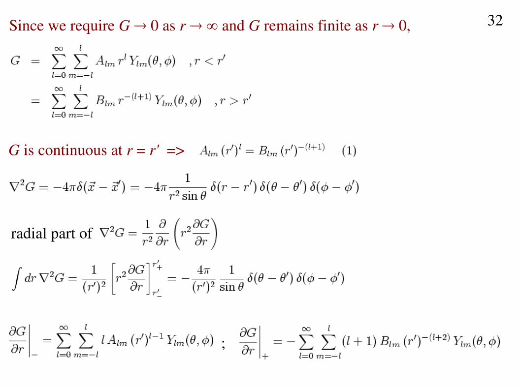
Since we require G  0 as r  ∞ and G remains finite as r  0,

G is continuous at r = r'  =>

radial part of

;

32

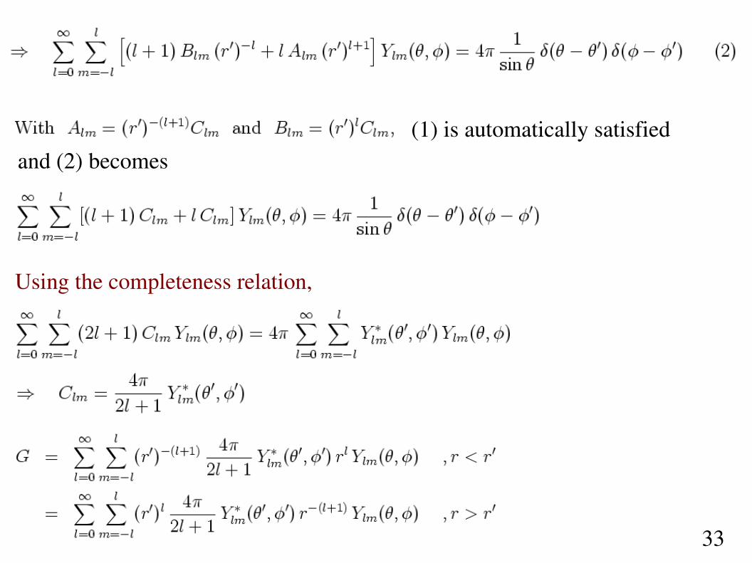
(1) is automatically satisfied and (2) becomes

Using the completeness relation,

33

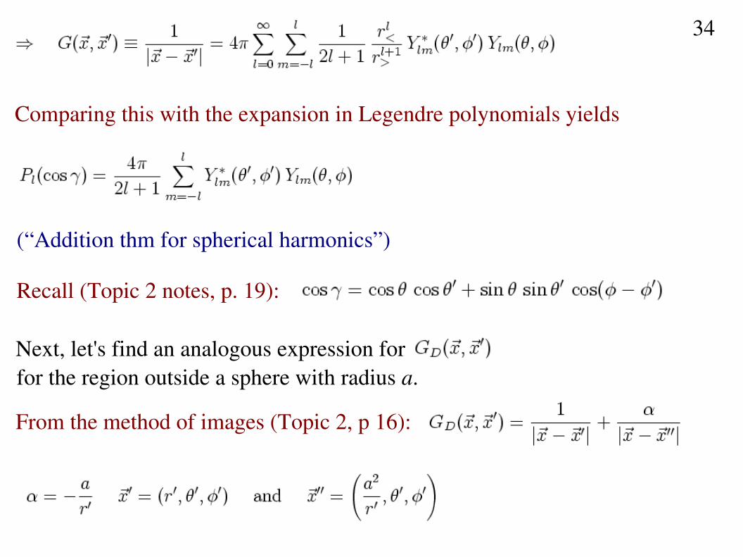
Comparing this with the expansion in Legendre polynomials yields

(“Addition thm for spherical harmonics”)

Recall (Topic 2 notes, p. 19):

Next, let's find an analogous expression forfor the region outside a sphere with radius a.

From the method of images (Topic 2, p 16):

34

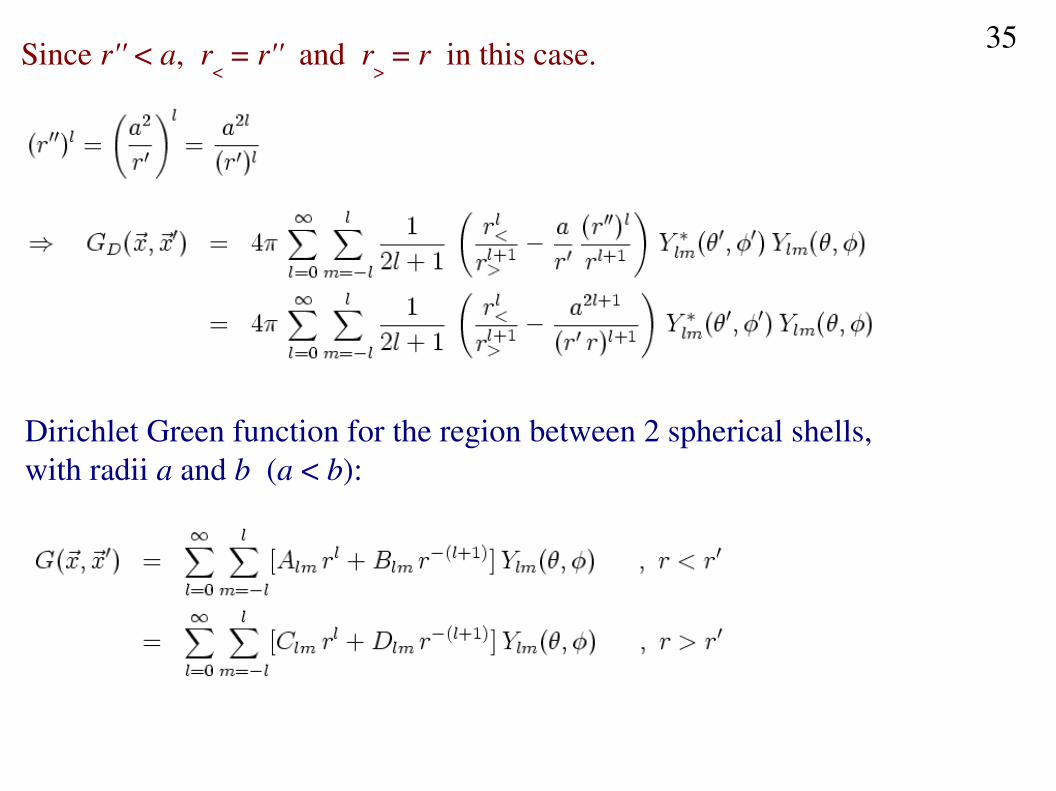
Since r'' < a,  r< = r''  and  r

> = r  in this case.

Dirichlet Green function for the region between 2 spherical shells, with radii a and b  (a < b):

35

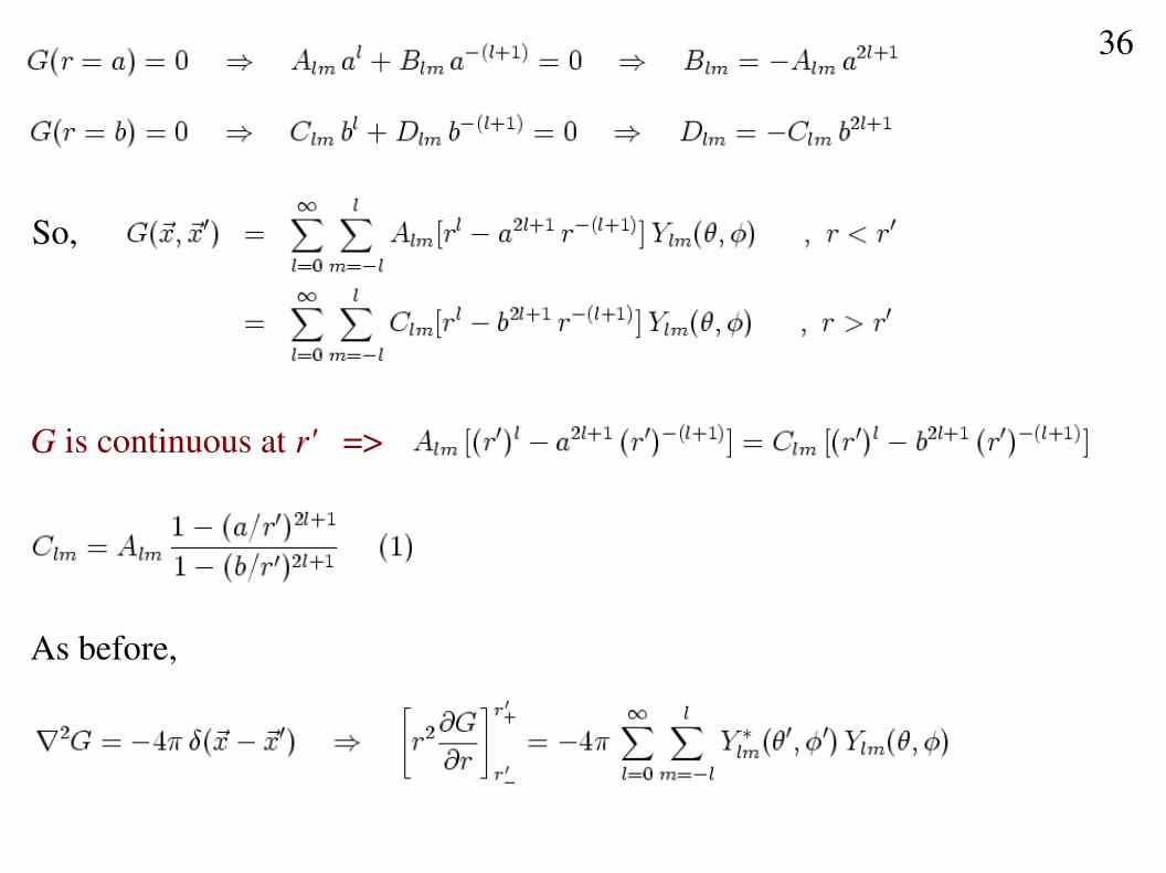
So,

G is continuous at r'   =>

As before,

36

=>

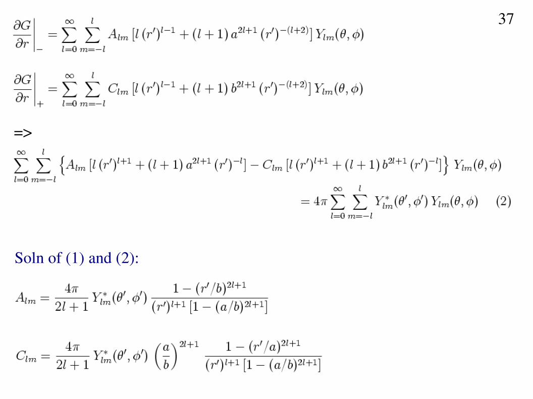
Soln of (1) and (2):

37

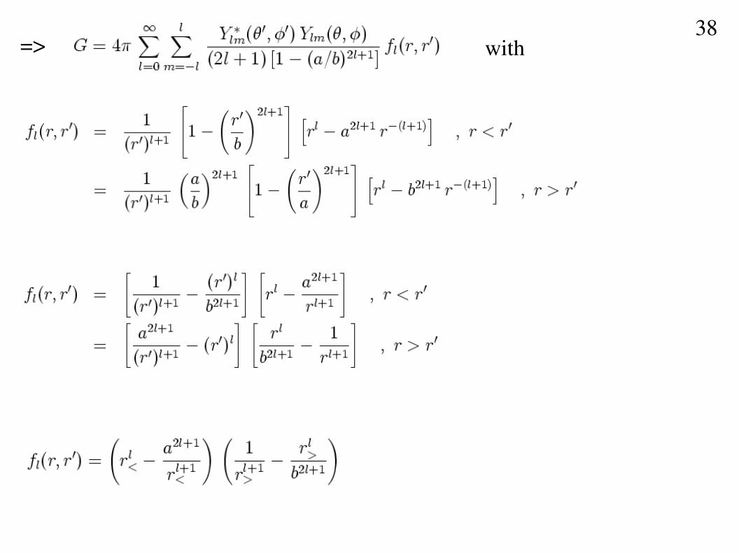
=> with38

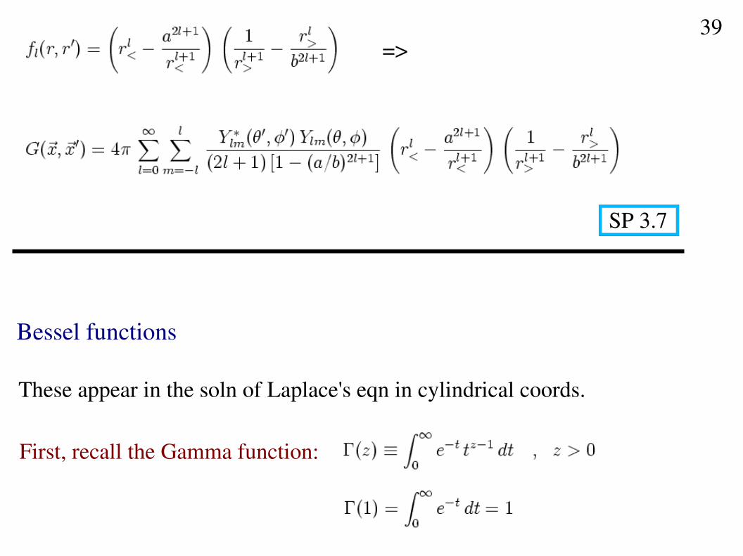
Bessel functions

These appear in the soln of Laplace's eqn in cylindrical coords.

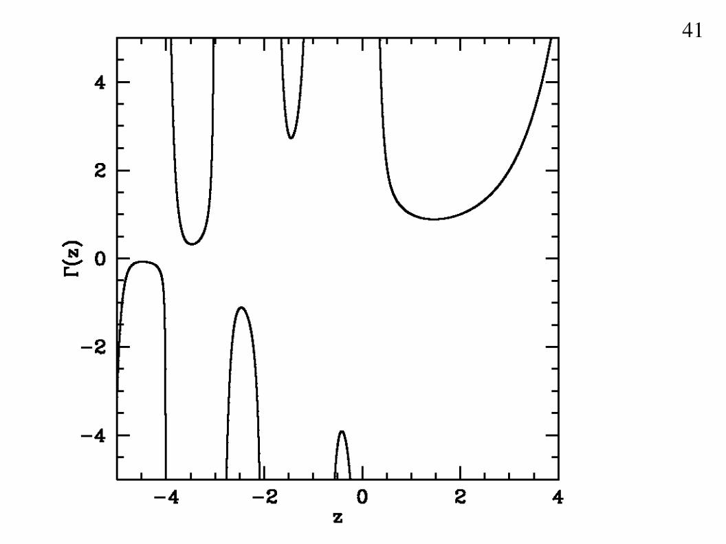
First, recall the Gamma function:

=>39

SP 3.7

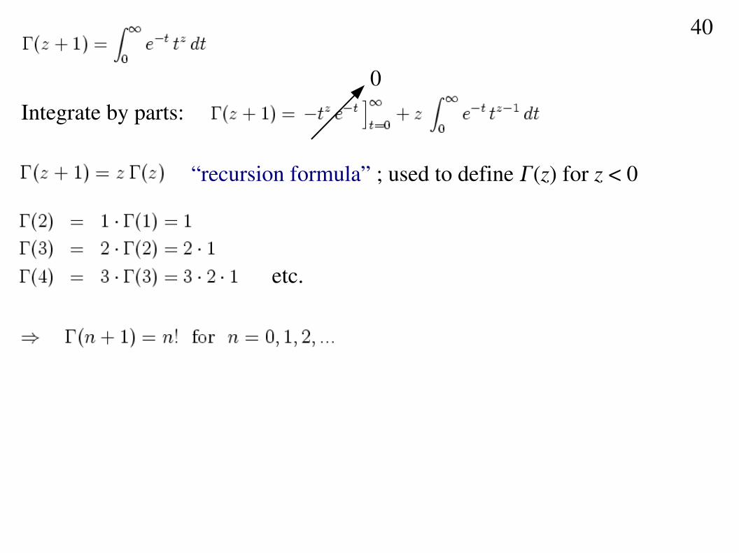
Integrate by parts:

0

“recursion formula” ; used to define (z) for z < 0

etc.

40

41

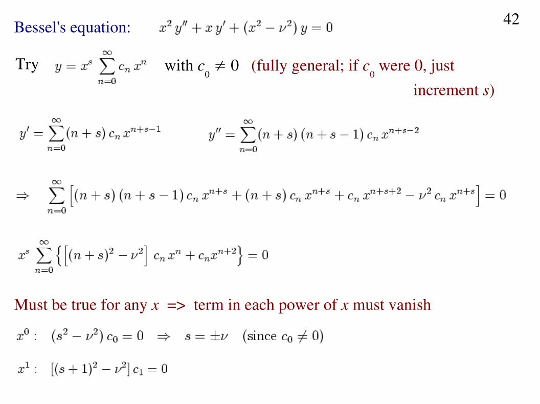
Bessel's equation:

Try with c0 ≠ 0   (fully general; if c

0 were 0, just            

                                                             increment s)

Must be true for any x  =>  term in each power of x must vanish

42

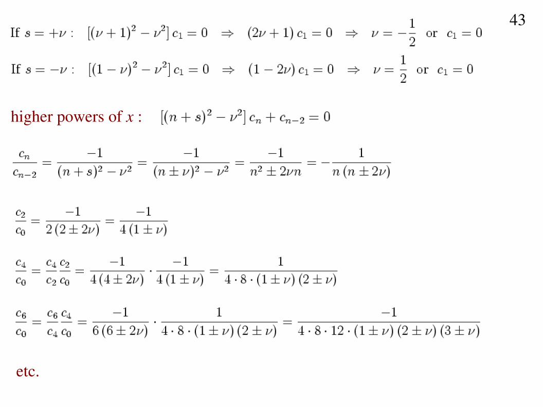
higher powers of x :

etc.

43

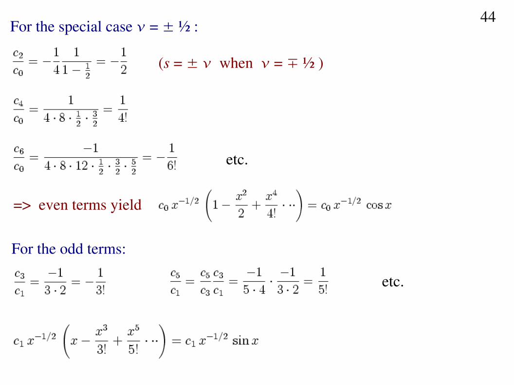
For the special case  = ± ½ :

(s = ±   when   = ∓ ½ )

etc.

=>  even terms yield

For the odd terms:

etc.

44

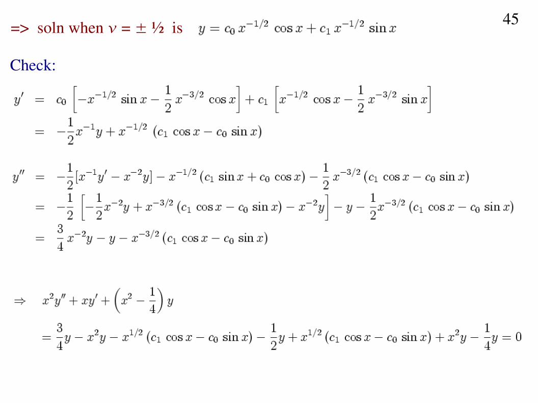
=>  soln when  = ± ½  is

Check:

45

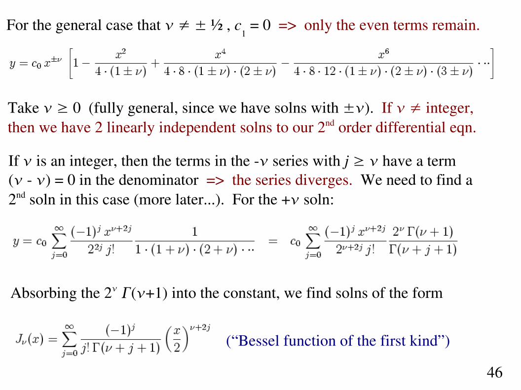
For the general case that  ≠ ± ½ , c1 = 0  =>  only the even terms remain.

Take  ≥ 0  (fully general, since we have solns with ±).  If  ≠ integer, then we have 2 linearly independent solns to our 2nd order differential eqn.

If  is an integer, then the terms in the ­ series with j ≥  have a term ( ­ ) = 0 in the denominator  =>  the series diverges.  We need to find a   2nd soln in this case (more later...).  For the + soln:

Absorbing the 2 (+1) into the constant, we find solns of the form

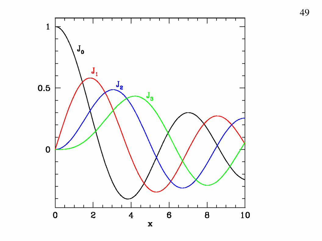
(“Bessel function of the first kind”)

46

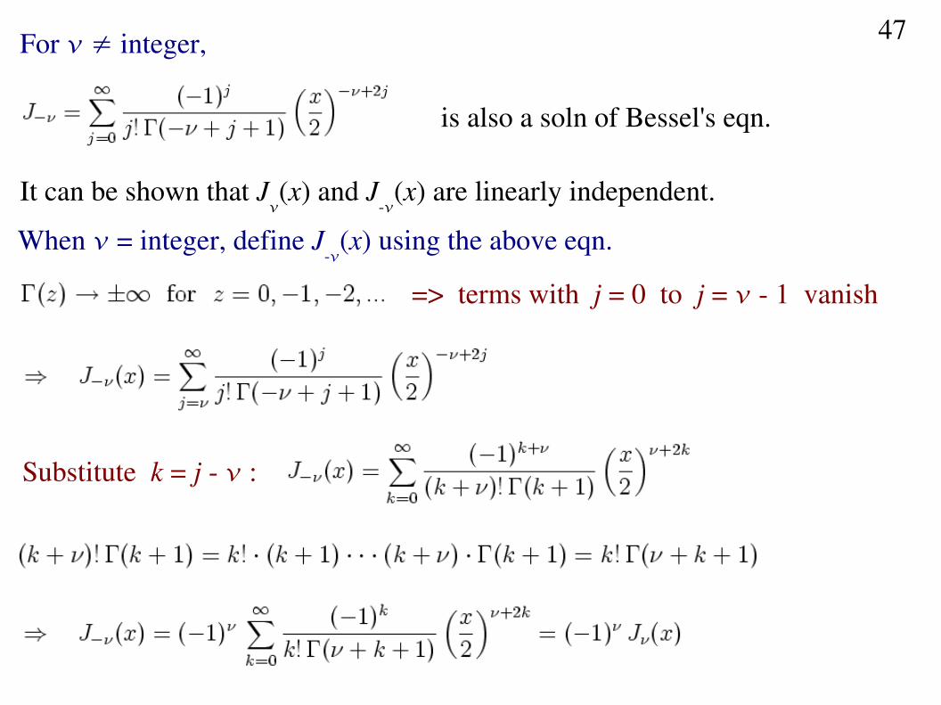
For  ≠ integer,

is also a soln of Bessel's eqn.

It can be shown that J(x) and J

­(x) are linearly independent.

 When  = integer, define J­

(x) using the above eqn.

=>  terms with  j = 0  to  j =  ­ 1  vanish

Substitute  k = j ­  :

47

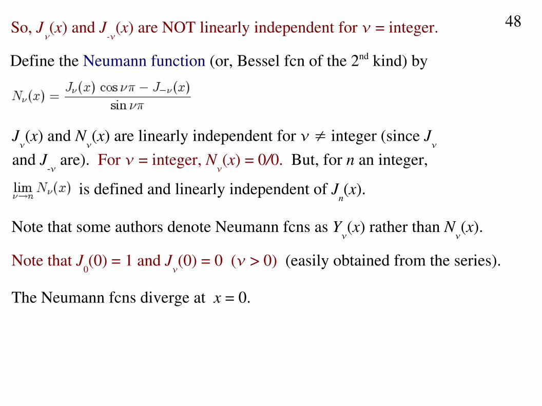
So, J(x) and J

­(x) are NOT linearly independent for  = integer.

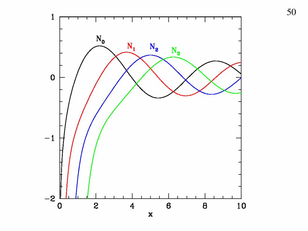
Define the Neumann function (or, Bessel fcn of the 2nd kind) by

J(x) and N

(x) are linearly independent for  ≠ integer (since J

 

and J­

 are).  For  = integer, N(x) = 0/0.  But, for n an integer, 

is defined and linearly independent of Jn(x).

Note that some authors denote Neumann fcns as Y(x) rather than N

(x).

Note that J0(0) = 1 and J

(0) = 0  ( > 0)  (easily obtained from the series).

The Neumann fcns diverge at  x = 0.

48

49

50

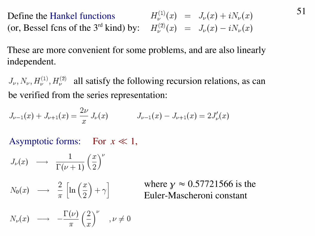
Define the Hankel functions (or, Bessel fcns of the 3rd kind) by:

These are more convenient for some problems, and are also linearly independent.

all satisfy the following recursion relations, as canbe verified from the series representation:

Asymptotic forms: For  x ≪ 1, 

where  ≈ 0.57721566 is the Euler­Mascheroni constant

51

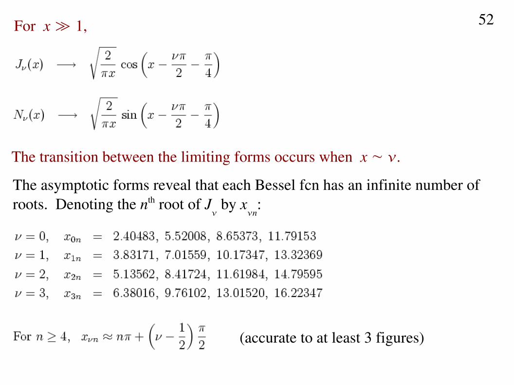
For  x ≫ 1, 

The transition between the limiting forms occurs when  x ~ .

The asymptotic forms reveal that each Bessel fcn has an infinite number of roots.  Denoting the nth root of J

 by x

n:

(accurate to at least 3 figures)

52

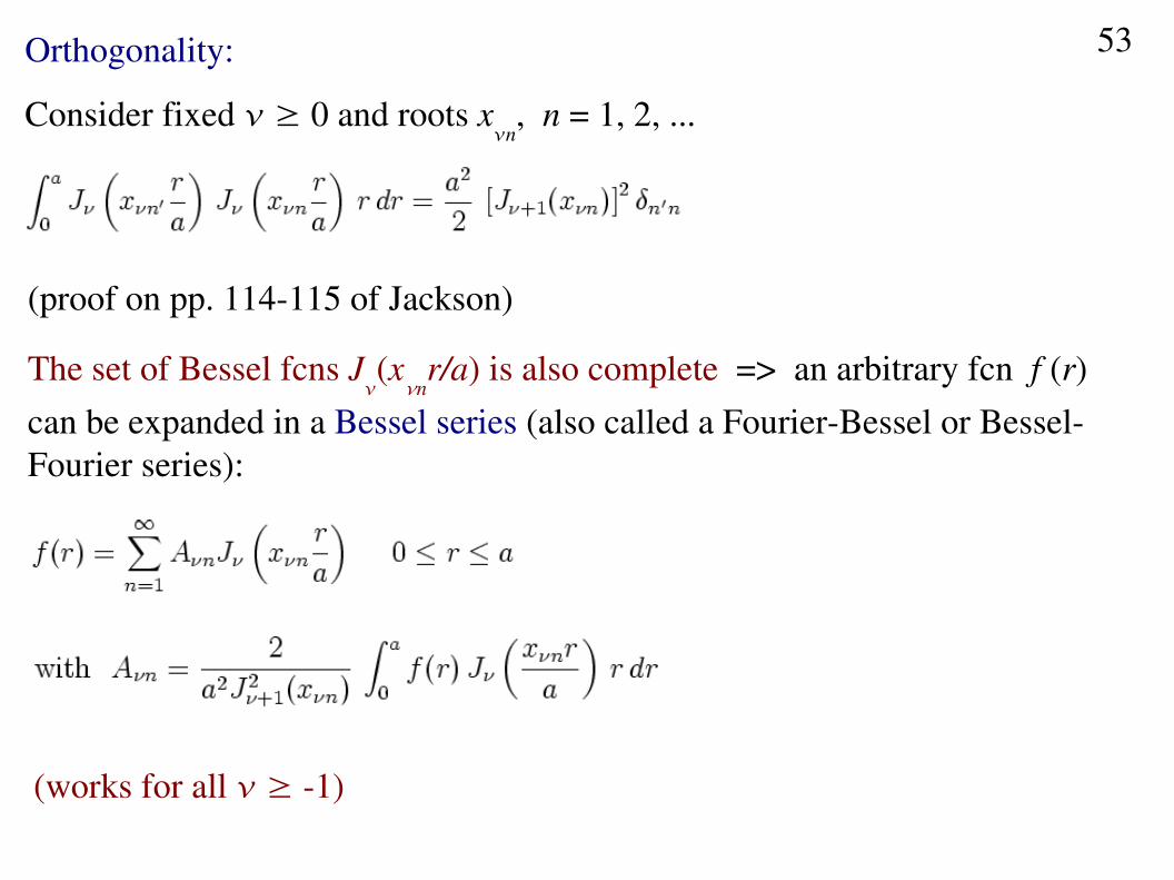
Orthogonality:

Consider fixed  ≥ 0 and roots xn

,  n = 1, 2, ...

(proof on pp. 114­115 of Jackson)

The set of Bessel fcns J(x

nr/a) is also complete  =>  an arbitrary fcn  f (r) 

can be expanded in a Bessel series (also called a Fourier­Bessel or Bessel­Fourier series):

(works for all  ≥ ­1)

53

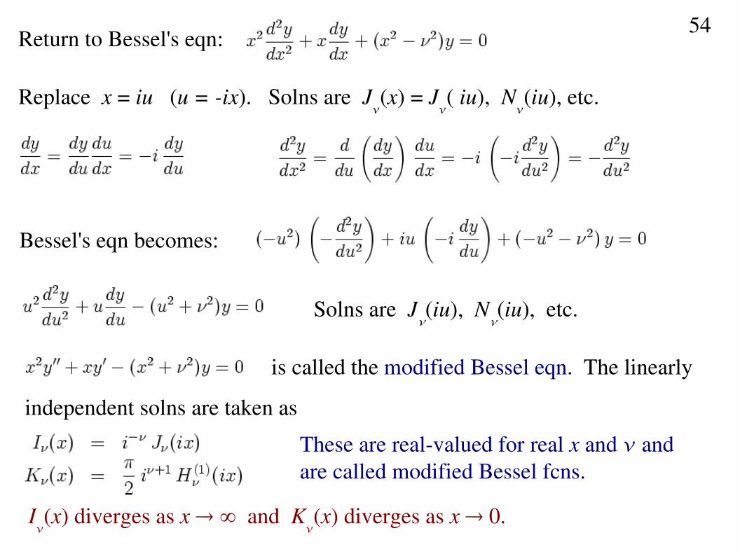
Return to Bessel's eqn:

Replace  x = iu   (u = ­ix).   Solns are  J(x) = J

( iu),  N

(iu), etc.

Bessel's eqn becomes:

Solns are  J(iu),  N

(iu),  etc.

is called the modified Bessel eqn.  The linearly

independent solns are taken as

These are real­valued for real x and  and are called modified Bessel fcns.

I(x) diverges as x  ∞  and  K

(x) diverges as x  0.

54

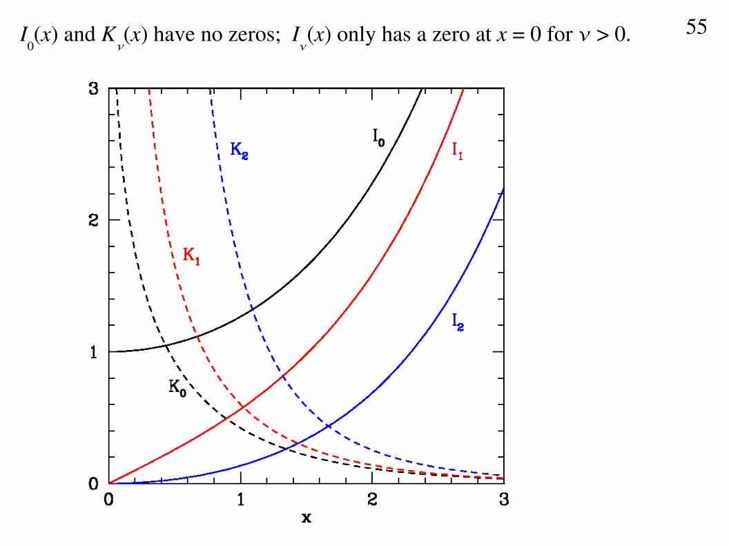
I0(x) and K

(x) have no zeros;  I

(x) only has a zero at x = 0 for  > 0.   55

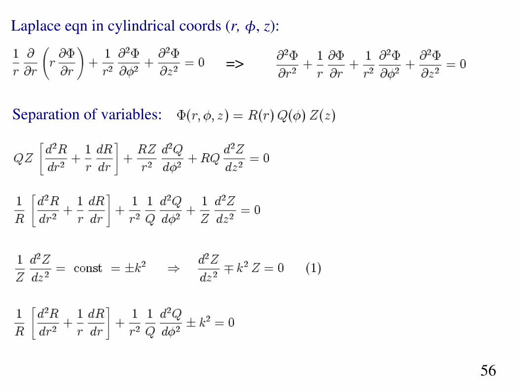
Laplace eqn in cylindrical coords (r, , z):

=>

Separation of variables:

56

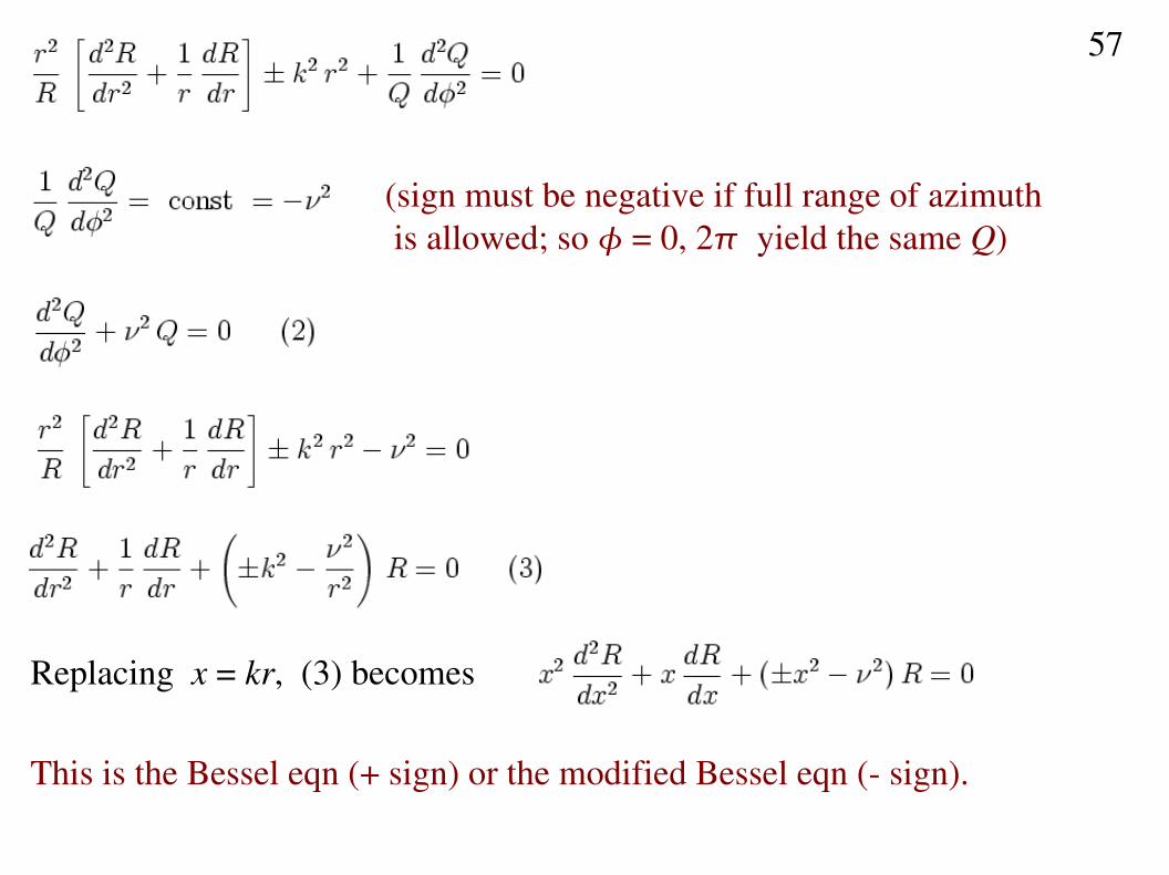
(sign must be negative if full range of azimuth  is allowed; so  = 0, 2 yield the same Q)

Replacing  x = kr,  (3) becomes

This is the Bessel eqn (+ sign) or the modified Bessel eqn (­ sign).

57

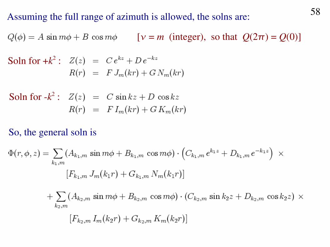
Assuming the full range of azimuth is allowed, the solns are:

[ = m  (integer),  so that  Q(2) = Q(0)]

Soln for +k2 :

Soln for ­k2 :

So, the general soln is

58

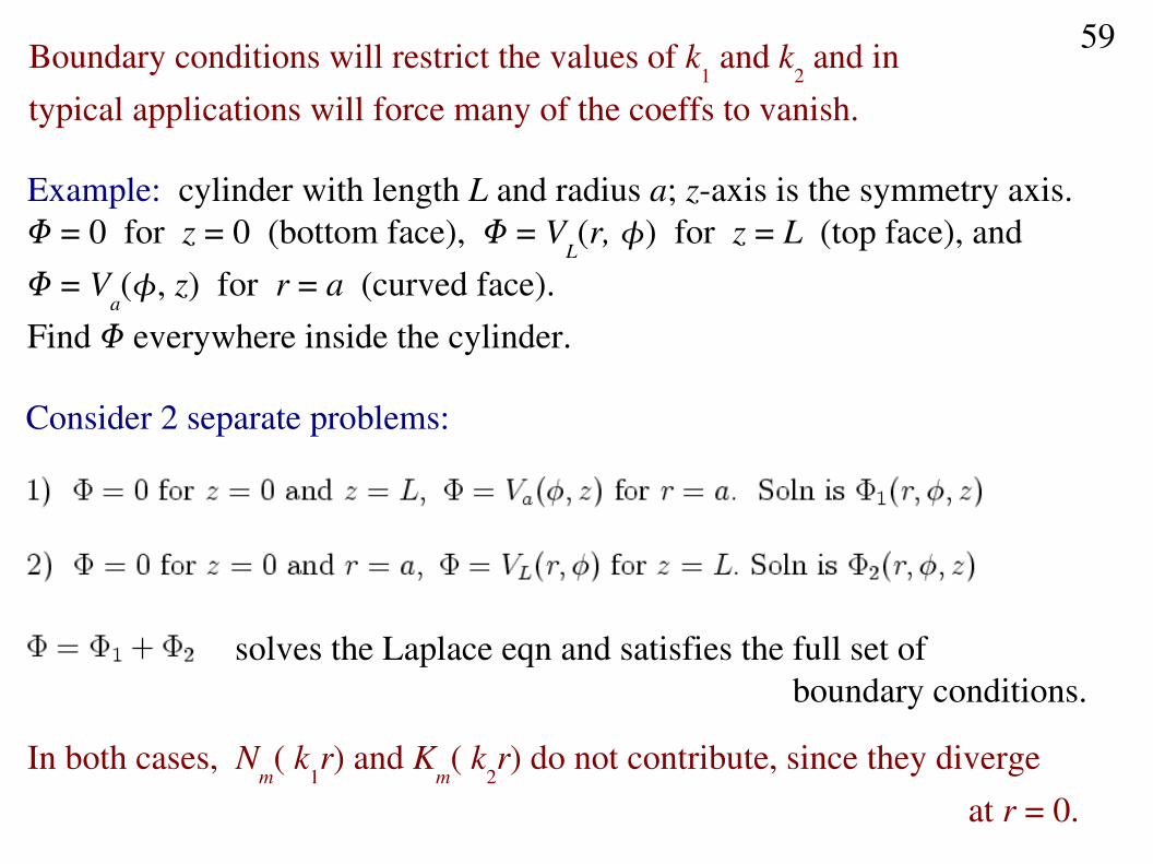
Boundary conditions will restrict the values of k1 and k

2 and in 

typical applications will force many of the coeffs to vanish.

Example:  cylinder with length L and radius a; z­axis is the symmetry axis. = 0  for  z = 0  (bottom face),   = V

L(r, )  for  z = L  (top face), and 

 = Va(, z)  for  r = a  (curved face).  

Find  everywhere inside the cylinder.

Consider 2 separate problems:

solves the Laplace eqn and satisfies the full set of                                                                boundary conditions.

In both cases,  Nm( k

1r) and K

m( k

2r) do not contribute, since they diverge

                                                                                                            at r = 0.

59

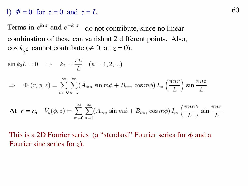
1)   = 0  for  z = 0  and  z = L

do not contribute, since no linearcombination of these can vanish at 2 different points.  Also, cos k

2z  cannot contribute (≠ 0  at  z = 0).

At  r = a,

This is a 2D Fourier series  (a “standard” Fourier series for  and aFourier sine series for z).

60

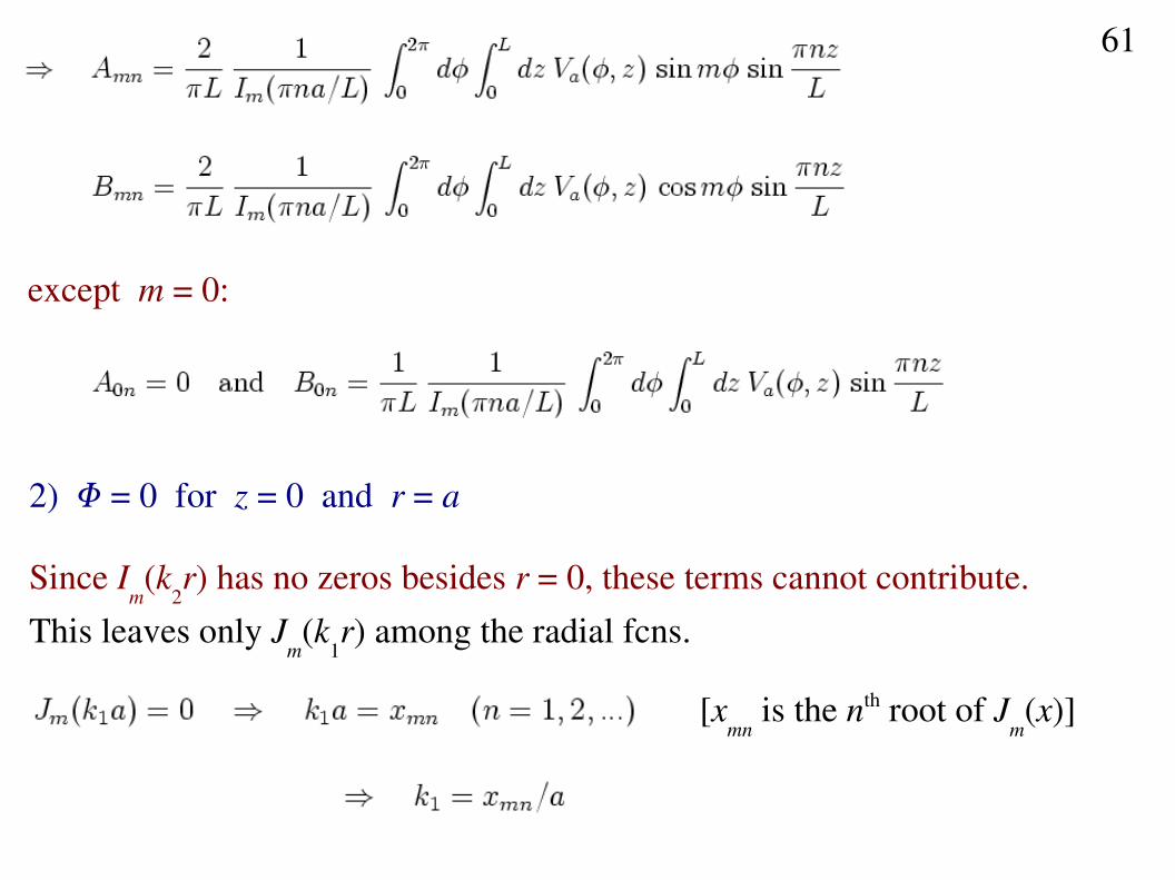
except  m = 0:

2)   = 0  for  z = 0  and  r = a

Since Im(k

2r) has no zeros besides r = 0, these terms cannot contribute.

This leaves only Jm(k

1r) among the radial fcns.

[xmn

 is the nth root of Jm(x)]

61

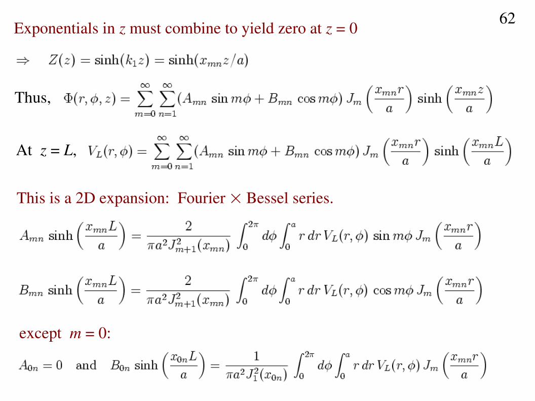
Exponentials in z must combine to yield zero at z = 0 

Thus,

At  z = L,

This is a 2D expansion:  Fourier × Bessel series.

except  m = 0:

62