251

10.1 Boundary Conditions

The boundary condition is the application of a force and/or constraint. In HyperMesh, boundary

conditions are stored within what are called load collectors. Load collectors may be created using the

right click context menu in the Model Browser (Create > Load Collector).

Quite often (especially at the beginning) a load collector is needed for the constraints (also called SPC

– Single Point Constraints) and a second one is needed for the forces and/or pressures. Keep in mind,

you can place any constraints (e.g. nodes constraint) with respect to dof 1, or nodes with constraints

dof123, etc. in a single load collector. The same rule applies for forces/pressures. They are stored

within a single load collector regardless of their orientiation and magnitude.

In the following you will learn some basic principles about the way forces may be applied to a structure.

1. Concentrated load (at a point or single node)

Force

Applying forces to single nodes may cause irritating e!ects, especially while looking at the stresses

in this area. Typically concentrated loads (i.e. forces on a single node) impose high stress gradients.

Even though the high stresses are correct (i.e. force applied to an in"nitesimal small area) one needs

to ask whether this kind of loading is reasonable at all? In other words, which real-life loading

scenario is represented in the model?

Therefore, forces are commonly applied as distributed loads, namely line loads, and surface loads

which are “closer” to reality.

X Boundary Conditions and Loads

This chapter includes material from the book “Practical Finite Element Analysis”. It also has been

reviewed and has additional material added by Matthias Goelke.

252

2. Force on line or edge

In the above "gure, a plate subjected to 10.000 N. The force is equally applied to all (11) nodes at the

model edge. Note that the forces at the corner will act only on ½ of the element edge.

The "gure above is a displacement contour plot. Note the red “hotspots” located in the corners of

the plate. The local displacement maximas are imposed by boundary e!ects (i.e. the forces applied

to the corner nodes act only on ½ of the element edge), however we applied a constant magnitude

along the plates edge.

In the example above, the plate is also subjected to 10.000 N. This time the forces at the corners are

just ½ the magnitude of the other applied forces.

253

The "gure above is the displacement contour plot from the plate_distributed.hm "le. The

displacements are more evenly distributed.

3. Traction (or “oblique” pressure)

Traction is a force acting on an area in any direction other than the normal direction. A force acting

normal to an area is known as pressure.

4. Distributed load (Force varying as equation)

How to apply a force with “variable” magnitude?

254

Distributed loads (varying with respects to the coordinates of the nodes or elements) can be applied

by means of an equation. In the displayed example, the magnitude of the applied forces varies with

respect to the nodal y-coordinate (i.e. the force is acting in negative z-direction and increases along

positive y-direction by a factor of 10 respectively).

5. Pressure and Vacuum

In the image above, a distributed load (pressure) is shown. The origin of the plate is located at the

highlighted node in the left upper corner.

How to apply a pressure with “variable” magnitude?

In the example above, the magnitude of the applied pressure depends on the x- and z- direction of

the elements centroid.

255

6. Hydrostatic pressure

Civil engineering applications: Dam design. Mechanical engineering applications: Vessels / tanks

containing liquid.

Hydrostatic pressure is zero at the top surface of the liquid and is maximum (= ρ* g * h) at the bottom

surface. It varies linearly as shown in the following "gure:

The hydrostatic pressure is applied taking into account the element centroids location (vertical

position, h).

7. Bending moments

The convention for representing a force is a single arrow ( ), pointed towards the direction of the

force .

A moment is represented by a double arrow, where the direction of the moment is decided by the

right hand rule.

The nodes along the plates edge are subjected to moments. As a consequence, the nodes will tend

to rotate with respect to the y-axis (dof 5).

256

In the image above, the plate is subjected to moments along its edge on the right. The

displacements are scaled by 100 and the initial model is displayed as wire frame.

The moment applied to the nodes in the "gure above can also be modeled by adding rigid elements

(RBE2) to each node which are then subjected to corresponding forces. In this example, the RBE2

would be oriented in the z-direction and subjected to a force acting in x-direction as shown in the

"gures below.

While postprocessing the results make sure that the RBE2 results (i.e. nodal position) are not

postprocessed (just display the displacements of the shell elements).

8. Torque:

257

What is torque? Are torque and bending moments di!erent?

Torque is a bending moment applied parallel to the axis of a shaft (Mx).

y

xz

Torque or Mx causes shear stresses and angular deformation, while the e!ect of the other two moments

(My , M

z) is the normal stress and longitudinal deformation.

How to decide the direction of torque (clockwise or anticlockwise)

It is based on the right hand rule. Point the thumb of your right hand towards the arrow direction. The

direction of your "ngers indicate the direction of torque.

y

xz

Torque Constraints

(clamped, 123456=0)

How to apply torque for solid elements (brick /tetra) :

As solid elements have no rotational sti!ness at the grid points (only 3 translational dofs), a common

mistake is to apply torques and moments to the grid points of solid elements directly.

The correct way to apply a moment to a solid model is to use an RBE2 or RBE3 rigid-body element. The

rigid-body element distributes an applied moment into the solid element model as forces.

Rigid element connection RBE2

A center node is connected to the outer edge nodes using a rigid element (RBE2). The torque is then

applied at the center node.

258

Alternatively, you may use an RBE3 elements instead:

Select the nodes at the outer contour of the shaft as independent nodes. The dependent node may

then be determined automatically. It is pretty easy.

However, care needs to be taken with respect to the dof’s being referenced. The node of the solid

shaft possess translational degrees of freedom only (dof 123). The dependent node also allows for

rotational displacements (dof 123456). If the rotational dof (in this example dof 5; rotation y-axis)

of the dependent node is not “activated”, the moment will not be transferred to the independent

nodes.

259

Shell element coating:

On the brick/tetra element outer face additional quad/tria (2-D) elements coating the solid elements

are created. The thickness of these shell element should be negligible (so that it would not a!ect the

results). Moment could now be applied on all the face nodes (moment per node = total moment / no.

of nodes on the face).

The shell element coating can be easily created within HyperMesh. Create faces using the Faces panel.

This panel can be accessed though the toolbar icon which is displayed using View > Toolbars >

Checks.

The faces (nothing more than 2-D plot elements) are automatically created and stored in a component

component collector, assign materials and properties)

260

In the "gure above, the elements of the shaft are displayed by means of the shrink element command

, . The orange elements are the hexahedral elements (3-D), and the red elements are the 2-D

elements placed on the free faces of the 3-D elements.

9. Temperature loading

Suppose a metallic ruler is lying on the ground freely as shown in the "gure below. If the temperature

of the room is increased to 50 degrees, would there be any stress in the ruler due to temperature?

There will be no stress in the ruler. It will just expand (thermal strain) due to the higher temperature.

Stress is caused only when there is a hindrance or resistance to deformation. Consider another case,

this time one end of the metallic object is "xed on a rigid wall (non conductive material). Now if the

temperature is increased, it will produce thermal stress (at the "xed end) as shown below.

For thermal stress calculations, the input data needed is the temperature value on nodes, the ambient

temperature, thermal conductivity, and the coe%cient of linear thermal expansion.

10. Gravity loading : Specify direction of gravity and material density.

261

A load collector with the card image GRAV is needed. Please keep your unit system in mind.

11. Centrifugal load

The user has to specify the angular velocity, axis of rotation, and material density as input data.

The RFORCE Card Image de"nes a static loading condition due to a centrifugal force "eld.

262

12. ‘g’ values (General rules) for full vehicle analysis :

Vertical acceleration (Impact due to wheel passing over speed braker or pot holes): 3g

Lateral acceleration (Cornering force, acts when vehicle takes a turn on curves): 0.5 to 1 g

Axial acceleration (Braking or sudden acceleration): 0.5 to 1 g

12. One wheel in ditch

The FE model should include all of the components (non critical components could be represented

by a concentrated mass). The mass of the vehicle and FE model mass, as well as actual wheel vehicle

reactions and FE model wheel reactions, should match.

While applying a constraint, the vertical dof of the wheel, which is in considered in the ditch, should

be released. The appropriate constraints should be applied on the other wheels so as to avoid rigid

body motion. Specify the gravity direction as downward and magnitude = 3*9810 mm/sec2

3 g

Another simple but approximate approach (since most of the time either we do not have all the CAD

data for the entire vehicle or su%cient time for a detailed FE model) is to apply 3 times the reaction

force on the wheel which is in the ditch. Suppose the wheel reaction (as per test data) is 1000 N.

Therefore, apply 3 * 1000 or 3000 N force in the vertically upward direction and constraint the other

three wheels enough to avoid rigid body motion. This approach works well for relative design (for

comparison of two designs).

13. Two wheels in ditch:

Same as discussed above, except now instead of one wheel, two wheels are in the ditch. One wheel in

the ditch causes twisting, while two wheels in the ditch produces a bending load.

3 g

3 g

14. Braking :

Linear acceleration (or gravity) along the axial direction (opposite to vehicle motion) = 0.5 to 1 g.

263

0.5 to 1 g

15. Cornering:

Linear acceleration along the lateral direction = 0.5 to 1 g.

0.5 to 1 g

10.2 How to Apply Constraints

A beginner may "nd it di%cult to apply boundary conditions, and in particular, constraints. Everyone

who starts a career in CAE faces the following two basic questions:

i) For a single component analysis, should forces and constraints be applied on the individual

component (as per the free body diagram) or should the surrounding components also be

considered.

ii) At what location and how many dof should be constrained.

Constraints (supports) are used to restrain structures against relative rigid body motions.

Supporting Two Dimensional Bodies

264

The "gure above depicts two-dimensional bodies that move in the plane of the paper (taken from:

http://www.colorado.edu/engineering/CAS/courses.d/IFEM.d/IFEM.Ch07.d/IFEM.Ch07.pdf).

If a body is not restrained, an applied load will cause in"nite displacements (i.e. the FEM program will

report a rigid body motion and will abort the run with an error message). Hence, regardless of loading

conditions, the body must be restrained against two translations along x and y, and one rotation

about z. Thus the minimum number of constraints that has to be imposed in two dimensions is three.

In "gure (a) above, the constraint at A "xes (pins) the body with respect to translational displacements,

whereas the constrain at B, together with A, provides rotational restraint. This body is free to distort in

any manner without the supports imposing any deformation constraints.

Figure (b) is a simpli"cation of "gure (a). Here the line AB is parallel to the global y-axis. The x and y

translations at point A, and the x translation at point B are restrained, respectively. If the roller support

at B is modi"ed as in "gure (c), a rotational motion about point A is possible (i.e. the rolling direction

is normal to AB). This will result in a singular modi"ed sti!ness matrix (i.e. rigid body motion).

Supporting Three Dimensional Bodies

The "gure above (taken from: http://www.colorado.edu/engineering/CAS/courses.d/IFEM.d/

IFEM.Ch07.d/IFEM.Ch07.pdf) illustrates the extension of the freedom restraining concept to three

dimensions. The minimal number of freedoms that have to be constrained is now six and many

combinations are possible.

In the example above, all three degrees of freedom at point A have been "xed. This prevents all rigid

body translations, and leaves three rotations to be taken care of. The x displacement component at

point B is constrained to prevent rotation about z, and the z component is "xed at point C toprevent

rotation about y. The y component is constrained at point D to prevent rotation about x.

1. Clutch housing analysis

Engine Clutch

housingTrans

case

265

The aim is to analyse (only) the clutch housing. The clutch housing is connected to the engine and

transmission case by bolts. There are 2 possibilities for analysis:

Approach 1) Only the clutch housing is considered for the analysis. Therefore, apply forces and

moments as per the free body diagram and constrain the bolt holes on both the side faces (all dof =

"x).

Approach 2) Model at least some portion of the engine and transmission case at the interface (otherwise

model both these components completely with a coarse mesh by neglecting small features). Then,

represent the other components like the front axle and rear axle using beam elements (approximate

the cross sections). Apply constraints at the wheels (not all the dof are "xed but only minimum dofs

required to avoid rigid motion or otherwise inertia relief / kinematic dof approach). Please note that

the clutch housing, being the critical area, should be meshed "ne.

The second option is recommended as the sti!ness representation, as well as constraints, are more

realistic. The "rst approach, "xing both sides of the clutch housing, results in over constraining and

will lead to safer results (less stress and displacement). Also, it is not possible to consider special load

cases like one wheel in ditch, two wheels in ditch, etc.

2. Bracket analysis

Problem de"nition: A bracket "xed in a rigid wall is subjected to a vertically downward load (180 kg).

Force

If above problem is given to CAE engineers working in di!erent companies then you will "nd di!erent

CAE engineers applying constraints di!erently:

i. Fix the bolt hole edge directly.

266

ii. Model the bolt using rigid / beam elements and clamp bolt end.

iii. Model the bolt, clamp bolt end, bracket bottom edge translations perpendicular to

surface "xed.

Stress

N/mm2

Displacement mm

Bolt holes edge �xed 993 15.5

Bolt – modeled by beam

elements

770 16.2

Bolt by beams and Bracket

bottom edge only z-dof �xed

758 15.8

Applying a direct constraint on the hole edge causes very high stress. The second method shows the

deformation of the bracket bottom edge, which is not realistic. Method 3 is recommended. Please

observe the di!erence in the magnitude of the stress and displacement.

In some organizations it is a standard practice to neglect stress at the washer layer elements (washer

area and one more layer surrounding the beam/rigid connection) due to high stresses observed at the

beam/rigid and shell/solid connections.

A modi"ed version of the bracket is depicted in the "gure below. This time the bracket is pinned to

the “wall” by means of 3 simpli"ed screws/bolts. The bolts are represented by rigid elements (RBE2).

The center of the rigid elements is "xed/constrained with respect to any translational displacements

267

(dof 1-3).

What would you expect to happen? Even though this kind of constraint seems reasonable (i.e.

bracket mounted to the wall), the unconstrained rotational dofs allow the central node to rotate.

Thus, the hole itself (even though the magnitude is very small) deforms (see "gure below).

In the "gure above, the displacements are scaled by 100. The undeformed shape is plotted in a

wireframe mode. Note the deformation of the hole. Is/was this e!ect really intended?

In the "gure above, the displacements are scaled by 100. The undeformed shape is plotted in a

wireframe mode. All the dofs of the central node are constrained. The hole remains its intial shape

and “position”.

Another illustrative example regarding the e!ects of the boundary constraints on the modelling

results is shown in the "gure below. The translationsal degrees of freedom (dof 123) of the nodes

at the rear end of the cantilever are constrained. At the tip a uniform force is applied in negative

x-direction.

268

What would you expect to happen, especially in the vicinity of the constraints?

In the "gure above, all the nodes at the rear are constrained with respect to any translational

displacements. The displacements in the y- and x-direction are scaled by a factor of 200 and 5,

respectively. The undeformed mesh is shown as wireframe (orange). Note the thickening at the

base of the cantilever accompanied with thinning at the top of the cantilever.

In the "gure above, there are modi"ed constraints at the rear of the cantilever. The nodes at the

rear part are constraint in the x- and z- direction. In addition, nodes located at the symmetry axis

(at the rear) are constraint in the y-direction. The displacements in the y- and x- direction are scaled

269

by a factor of 200 and 5, respectively. The undeformed mesh is shown as wireframe (orange). The

displacements are quite di!erent compared to the earlier "gure. The question to be answered is

which model is correct?

Imposing boundary conditions (constraints and forces) by means of RBE2 and RBE3. What are

the di!erences?

In the "gure above, the nodes at the hole are constrained by an RBE2 element where the

independent node is "xed with respect to all degrees of freedom (dof123456).

Before looking at the simulation results, ask yourself, what will the displacement contours look like?

The "gure above is a plot of the displacement "eld. Note that the displacements at the hole are zero.

In other words, the RBE2 element “arti"cially” sti!ens the hole.

Next, we are constraining the model by means of a RBE3 element. Note, that the dependent node of

the RBE3 element (i.e. the one in the center of the spider) can’t be constraint directly. This is because

this node would depend on the nodes at the hole and the SPC. A work around is to attach the

dependent node to a CBUSH element (with zero length and high sti!ness values). The free node of

the CBUSH element is then constrained with respect to all degrees of freedom.

270

The above "gure illustrates how the dependent node of the RBE3 is grounded to an CBUSH element

with zero length. All degress of freedom of the free node of the CBUSH are constrained. CBUSH

elements are created in the spring panel which can be accessed by selecting Mesh > Create > 1D

Elements > Springs.

In order to create CBUSH elements, you "rst need to determine the corresponding “elem types”

(default is CELAS), reference a property (can also be assigned later), and select the two end nodes of

the spring. The options dof1-6 are irrelevant.

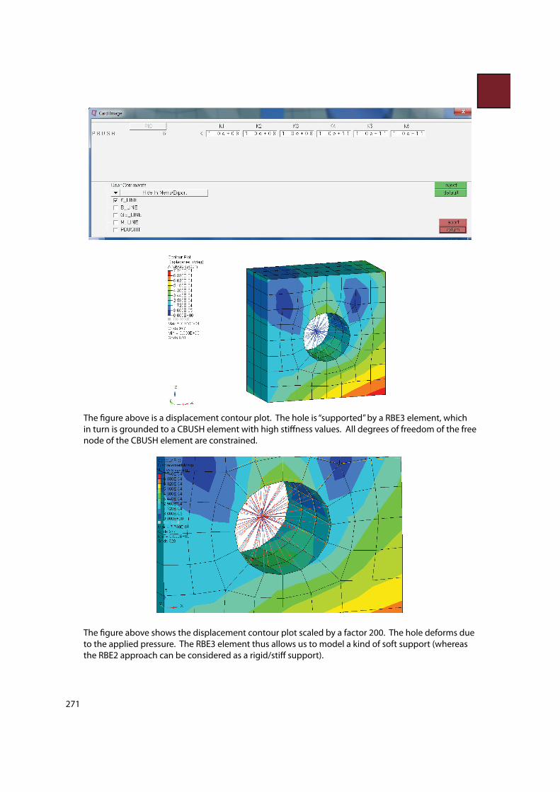
The property de"nition of the CBUSH element is shown in the following image

271

The "gure above is a displacement contour plot. The hole is “supported” by a RBE3 element, which

in turn is grounded to a CBUSH element with high sti!ness values. All degrees of freedom of the free

node of the CBUSH element are constrained.

The "gure above shows the displacement contour plot scaled by a factor 200. The hole deforms due

to the applied pressure. The RBE3 element thus allows us to model a kind of soft support (whereas

the RBE2 approach can be considered as a rigid/sti! support).

272

3. Pressure vessel lying freely on the ground and plate subjected to tensile load on both the

sides

Sometimes a situation demands for an unconstrained structural analysis like a pressure vessel

lying freely on the ground (just placed, no constraint/"xing) or a plate subjected to tensile load

on the opposite edges without any constraint. A static analysis problem cannot be solved for an

unconstrained structure. It should be "xed at atleast one node, or alternatively, at a few nodes so as

to restrict rigid body motion.

If the problem of the pressure vessel (subjected to internal pressure) or the plate with tensile load is

solved without specifying any constraints, then either the solver will quit giving a singularity error

message or otherwise report very that there is a high stress at an unrealistic location (if the auto

singularity option is switched on).

To solve an unconstrained structural problems there are 2 ways:

1) Approximate approach: Create spring / beam elements (negligible sti!ness value) on

the entire circumference (outer edges or surface nodes) and apply the constraint at the

free end of spring or beam.

2) Recommended : Inertia relief method or de"ning kinematic dofs in the model (see

tutorial RD-1030: 3D Inertia Relief Analysis using RADIOSS)

273

10.3 Symmetry

Symmetry

Plane

symmetry

Anti

symmetry

Axial

symmetry

Cyclic

symmetry

Condition for using any type of symmetry

Symmetric conditions could be used only when both the following conditions are ful"lled.

1) Geometry is symmetric

2) Boundary conditions (forces and constraints) are symmetric.

Advantages: Half, quarter or a portion of the model could be used for analysis, resulting in fewer dofs

and computational cost.

Which dof must be constrained at the symmetry level?

In the "gure above, the dark vertically oriented plane represents the plane of symmetry. The "nite

elements nodes are colored gray, whereas possible nodal rotations are shown by means of blue,

green and red arrows. Nodal rotations with respect to the green and red axis/arrows would “move/

rotate” the node out of the plane of symmetry (just imagine the arrows would be glued to the nodes).

Hence these degree of freedoms (dof ) must be constrained. In contrast, nodal rotations with respect

to the blue axis/arrow are not needed to be constrained. As the nodes of solid elements do only allow

translational displacements, one just need to constrain any out of symmetry plane motions.

274

The "gure above is considered the full model. The beam ends are constrained with respect to any

translational displacements (dof 123). A vertical load of 200 N is applied at its center.

If the symmetry plane is in the x-y plane then the translational displacements in its normal direction

i.e. z-direction (dof 3) need to be constrained. On the other hand, we don’t need to "x/delete rotations

with respect to z-axis as solid elements do not allow nodal rotations. Remember, the nodes at the

symmetry plane are not allowed to move (or rotate) out of the plane of symmetry.

The "gure above is considered the half model . At the plane of symmetry, the z-displacements (dof 3)

are constrained. In addition, the original force is divided by two (as it acts only on half of the structure).

275

Let us consider a symmetrical plate with a hole subjected to symmetrical loads on the two opposing

edges.

The "gure above is the full plate model and serves as a reference model

The "gure above is a contour plot of the element stresses (von Mises).

In the next step, a quarter segment of the plate is investigated. T he corresponding loads and

constraints are depicted in the "gure below.

276

The "gure above is a contour plot of the element stresses (von Mises).

Limitations: Symmetric boundary conditions should not be used for dynamic analysis (natural

frequency and modal superposition solver). A symmetric model (half or portion of part) would miss

some of the modes (anti nodes or out of phase modes) as shown below:

Natural Frequency comparison for Full and Half symmetric model

277

Mode No. Full model

Hz

Half symmetric model

Hz

1 448 448

2 449 718

3 718 1206

4 719 2078

5 1206 2672

6 1211 4397

Question : We need to do a simulation of a casting component to decide the best option out of

two casting materials. What will be the di!erentiating parameters, since the modulus of elasticity and

poisson’s ratio for both of the materials are the same. Secondly, we do not have stress strain data for

both of the materials.

1) If the nature of the loading is static (most of the time static and rarely dynamic) and the

company has only a linear static solver : Di!erent grades of cast iron have di!erent ultimate

strength (or proportional yield strength). Linear static stress is independent of material and both the

materials would report the same stress. The decision could be made based on the ultimate strength

(and endurance strength). Say the maximum stress as per the FEA is 300 N/mm2. For material 1, the

ultimate stress is 350 and for material 2 it is 500 N/mm2. In this situation, the second material is clearly

the choice. Consider another case. Suppose the maximum stress reported by the FEA is 90. One can

calculate the approximate value of endurance strength. For grey cast iron, the endurance strength =

0.3 * ultimate strength. Therefore, for material 1 the endurance strength is 105 N/mm2 and should be

preferred over the second one.

2) If the nature of the loading is dynamic and subjected to a sever load : Fatigue analysis is strongly

recommended. Commercial fatigue analysis software usually provide material library. Specifying the

appropriate material grade, surface "nish, etc. and calculations for the life / endurance factor of safety

would lead to realistic and optimum selection out of the two options.

10.4 Creating Loadsteps in HyperMesh

And "nally, once the constraints and loads are speci"ed, a corresponding loadstep needs to be

created (otherwise the Finite Element program would not know what to do with these entities). In

HyperMesh, this is done by selecting Setup > Create > LoadSteps.

10.4 Creating Loadsteps in HyperMesh

278

The image aboves shows the Load Step panel in HyperMesh. This panel is used to de"ne a loadstep.

First, speci"y the name and the type of the loadstep. The load collector with the constraints are

referenced using SPC and the forces/pressure are referenced using LOAD.

The loadstep will then be listed in the Model Browser along with all the other model entities.

Now the model can be exported and the analysis can be started!

10.5 Tutorials and Interactive Videos

To view the following videos and tutorials, you "rst need to register at the HyperWorks Client Center

using your university E-Mail address. Once you have a password, log into the Client Center and then

access the videos and tutorials using the links below.

Recommended Tutorials:

These tutorials can be accessed within the installation inside the Help Document.:

From the menu bar select Help > HyperWorks Desktop > Tutorials > HyperWorks Tutorials >

HyperWorks Desktop > HyperMesh > Analysis Setup.

Tutorials can also be accessed within the Online Help which can be accessed using the links below.

You will need to log into the HyperWorks Client Center to access these tutorials online.

HM-4000: Setting up Loading Conditions

HM-4040: Working with Loads on Geometry

Recommended Videos

Product Videos (10-15 minute; no HyperWorks installation required)

How to apply loads and constraints?

How to de"ne a load step?

Recommended Tips and Tricks

Boundary Conditions – Loads Summary Tool

Beam - Pressure Loading

Presentation

Suspension and Chassis Loads

10.5 Tutorials and Interactive Videos