boston university college of engineering dissertation
TRANSCRIPT

BOSTON UNIVERSITY
COLLEGE OF ENGINEERING
Dissertation
ACTIVE SCENE ILLUMINATION METHODS FOR
PRIVACY-PRESERVING INDOOR OCCUPANT
LOCALIZATION
by
JINYUAN ZHAO
B.S., Tsinghua University, 2015
Submitted in partial fulfillment of the
requirements for the degree of
Doctor of Philosophy
2019

c© 2019 byJINYUAN ZHAOAll rights reserved

Approved by
First Reader
Prakash Ishwar, Ph.D.Professor of Electrical and Computer EngineeringProfessor of Systems Engineering
Second Reader
Janusz L. Konrad, Ph.D.Professor of Electrical and Computer Engineering
Third Reader
Vivek Goyal, Ph.D.Associate Professor of Electrical and Computer Engineering
Fourth Reader
Thomas D.C. Little, Ph.D.Associate Dean of Educational InitiativesProfessor of Electrical and Computer EngineeringProfessor of Systems Engineering

Acknowledgments
First and foremost, I would like to express my gratitude to my research advisor,
Prof. Prakash Ishwar, and my co-advisor, Prof. Janusz Konrad for their support
and guidance. During my PhD study, they offered me a lot of help in shaping my
research problem and identifying key questions, designing experiments to support a
conclusion, finding interesting directions to move my research forward, preparing for
oral and poster presentations, and establishing good habits to keep things organized.
Also, I would like to thank for their enormous time and effort devoted to revising and
organizing drafts of my papers, presentation slides and posters. I especially appreciate
Prof. Ishwar for his valuable insights, patience and care for my personal growth and
career development. It has been really fortunate to work with them. I would also
like to thank other members of my committee, Prof. Vivek Goyal and Prof. Thomas
Little, for their valued feedback and suggestions.
Apart from my committee members, I would also like to express my thanks to
my collaborator, Natalia Frumkin. She spent a huge amount of time in configuring
and debugging our physical testbed, assisting me with all the testbed experiments,
and coordinating with the ECE Senior Design team ActiLocate. My thanks also go
to members of team ActiLocate – William Chen, Hannah Gibson, Tu Timmy Hoang,
Dong Hyun Kim and Adam Surette – for delivering a functional testbed that met our
design requirements.
I would also like to acknowledge some of the current and former members of BU
College of Engineering who made my life in Boston more enjoyable: Jiawei Chen,
Christy Lin, Rui Chen, Ruidi Chen, Tingting Xu, Henghui Zhu, Dr. Nan Zhou,
Ozan Tezcan, Kubra Cilingir, Dr. Jonathan Wu and Xizhi Wu. Their generous help,
support and encouragement made me feel at home.
Finally, a special thanks go to my parents and family for their love and support.
iv

They encouraged and helped me in going through the hard times in my life, and
without them I would not have achieved what I have today.
This work was supported by the NSF under ERC Cooperative Agreement No.
EEC-0812056 and Boston University’s Undergraduate Research Opportunities Pro-
gram. Any opinions, findings, and conclusions or recommendations expressed are
those of the author(s) and do not necessarily reflect the views of the sponsors.
v

ACTIVE SCENE ILLUMINATION METHODS FOR
PRIVACY-PRESERVING INDOOR OCCUPANT
LOCALIZATION
JINYUAN ZHAO
Boston University, College of Engineering, 2019
Major Professors: Prakash Ishwar, Ph.D.Professor of Electrical and Computer EngineeringProfessor of Systems Engineering
Janusz L. Konrad, Ph.D.Professor of Electrical and Computer Engineering
ABSTRACT
Indoor occupant localization is a key component of location-based smart-space
applications. Such applications are expected to save energy and provide produc-
tivity gains and health benefits. Many traditional camera-based indoor localization
systems use visual information to detect and analyze the states of room occupants.
These systems, however, may not be acceptable in privacy-sensitive scenarios since
high-resolution images may reveal room and occupant details to eavesdroppers. To
address visual privacy concerns, approaches have been developed using extremely-
low-resolution light sensors, which provide limited visual information and preserve
privacy even if hacked. These systems preserve visual privacy and are reasonably
accurate, but they fail in the presence of noise and ambient light changes.
This dissertation focuses on two-dimensional localization of an occupant on the
floor plane, where three goals are considered in the development of an indoor localiza-
vi

tion system: accuracy, robustness and visual privacy preservation. Unlike techniques
that preserve user privacy by degrading full-resolution data, this dissertation focuses
on an array of single-pixel light sensors. Furthermore, to make the system robust to
noise, ambient light changes and sensor failures, the scene is actively illuminated by
modulating an array of LED light sources, which allows algorithms to use light trans-
ported from sources to sensors (described as light transport matrix) instead of raw
sensor readings. Finally, to assure accurate localization, both principled model-based
algorithms and learning-based approaches via active scene illumination are proposed.
In the proposed model-based algorithm, the appearance of an object is modeled as
a change in floor reflectivity in some area. A ridge regression algorithm is developed
to estimate the change of floor reflectivity from change in the light transport matrix
caused by appearance of the object. The region of largest reflectivity change identifies
object location. Experimental validation demonstrates that the proposed algorithm
can accurately localize both flat objects and human occupants, and is robust to noise,
illumination changes and sensor failures. In addition, a sensor design using aperture
grids is proposed which further improves localization accuracy. As for learning-based
approaches, this dissertation proposes a convolutional neural network, which reshapes
the input light transport matrix to take advantage of spatial correlations between
sensors. As a result, the proposed network can accurately localize human occupants
in both simulations and the real testbed with a small number of training samples.
Moreover, unlike model-based approaches, the proposed network does not require
modeling assumptions or knowledge of room, sources and sensors.
vii

Contents
1 Introduction 1
1.1 Background . . . . . . . . . . . . . . . . . . . . . . . . . . . . . . . . 1
1.2 Related work . . . . . . . . . . . . . . . . . . . . . . . . . . . . . . . 4
1.2.1 Wearable-beacon-based systems . . . . . . . . . . . . . . . . . 4
1.2.2 Beaconless systems . . . . . . . . . . . . . . . . . . . . . . . . 5
1.2.3 Visual privacy preservation . . . . . . . . . . . . . . . . . . . . 6
1.3 Contributions . . . . . . . . . . . . . . . . . . . . . . . . . . . . . . . 7
1.3.1 System framework . . . . . . . . . . . . . . . . . . . . . . . . 9
1.3.2 Model-based localization approaches . . . . . . . . . . . . . . 10
1.3.3 Data-driven localization approaches . . . . . . . . . . . . . . . 11
1.3.4 Experimental Validation . . . . . . . . . . . . . . . . . . . . . 12
1.3.5 Other findings . . . . . . . . . . . . . . . . . . . . . . . . . . . 13
1.4 Organization . . . . . . . . . . . . . . . . . . . . . . . . . . . . . . . 13
2 Model-based indoor localization via passive scene illumination 14
2.1 Light reflection model . . . . . . . . . . . . . . . . . . . . . . . . . . 14
2.2 Localization via passive illumination . . . . . . . . . . . . . . . . . . 17
2.3 Experiments . . . . . . . . . . . . . . . . . . . . . . . . . . . . . . . . 19
2.3.1 Experimental setup . . . . . . . . . . . . . . . . . . . . . . . . 20
2.3.2 Simulation Experiments . . . . . . . . . . . . . . . . . . . . . 21
2.3.3 Testbed Experiments . . . . . . . . . . . . . . . . . . . . . . . 26
2.4 Summary . . . . . . . . . . . . . . . . . . . . . . . . . . . . . . . . . 29
viii

3 Model-based indoor localization via active scene illumination 30
3.1 Active illumination methodology . . . . . . . . . . . . . . . . . . . . 30
3.2 Obtaining light transport matrix A . . . . . . . . . . . . . . . . . . . 34
3.3 Localization via active illumination . . . . . . . . . . . . . . . . . . . 35
3.3.1 LASSO algorithm . . . . . . . . . . . . . . . . . . . . . . . . . 36
3.3.2 Localized ridge regression algorithm . . . . . . . . . . . . . . . 37
3.3.3 Comparison of LASSO and Localized ridge regression algorithms 40
3.4 Comparison with localization via passive illumination . . . . . . . . . 43
3.4.1 Simulation and testbed experiments . . . . . . . . . . . . . . . 43
3.4.2 Discussion . . . . . . . . . . . . . . . . . . . . . . . . . . . . . 48
3.5 Localization of humans . . . . . . . . . . . . . . . . . . . . . . . . . . 49
3.5.1 Experimental setup . . . . . . . . . . . . . . . . . . . . . . . . 49
3.5.2 Simulation and testbed experiments . . . . . . . . . . . . . . . 52
3.6 3D, moving and multiple object localization . . . . . . . . . . . . . . 55
3.6.1 Shadow-based 3D object localization . . . . . . . . . . . . . . 55
3.6.2 Moving object localization . . . . . . . . . . . . . . . . . . . . 61
3.6.3 Multiple object localization . . . . . . . . . . . . . . . . . . . 63
3.7 Estimation of light contribution matrix C . . . . . . . . . . . . . . . 65
3.7.1 Sampling of matrix C . . . . . . . . . . . . . . . . . . . . . . 65
3.7.2 Estimating C from samples on a lattice . . . . . . . . . . . . . 70
3.7.3 Experimental results . . . . . . . . . . . . . . . . . . . . . . . 74
3.7.4 Conclusions . . . . . . . . . . . . . . . . . . . . . . . . . . . . 77
3.8 Localization with apertures on light sensors . . . . . . . . . . . . . . 78
3.9 Summary . . . . . . . . . . . . . . . . . . . . . . . . . . . . . . . . . 84
4 Data-driven approaches to indoor localization via active scene illu-
mination 86
ix

4.1 Classical data-driven approaches . . . . . . . . . . . . . . . . . . . . . 87
4.1.1 Support vector regression (SVR) . . . . . . . . . . . . . . . . 87
4.1.2 K-nearest neighbor (KNN) regression . . . . . . . . . . . . . . 89
4.2 Convolutional neural network (CNN) approach . . . . . . . . . . . . . 90
4.3 Experimental results . . . . . . . . . . . . . . . . . . . . . . . . . . . 92
4.3.1 Simulation experiments . . . . . . . . . . . . . . . . . . . . . . 93
4.3.2 Testbed experiments . . . . . . . . . . . . . . . . . . . . . . . 95
4.4 Transfer learning . . . . . . . . . . . . . . . . . . . . . . . . . . . . . 96
4.5 Robustness to sensor failures . . . . . . . . . . . . . . . . . . . . . . . 100
4.6 Summary . . . . . . . . . . . . . . . . . . . . . . . . . . . . . . . . . 102
5 Conclusions 103
5.1 Summary of the dissertation . . . . . . . . . . . . . . . . . . . . . . . 103
5.2 Future directions . . . . . . . . . . . . . . . . . . . . . . . . . . . . . 105
A Closed-form Solution to Ridge Regression Problem 106
References 107
Curriculum Vitae 113
x

List of Tables
2.1 Dimensions of rectangular objects used in experiments. . . . . . . . . 21
2.2 Localization errors of the passive illumination algorithm in MATLAB
simulation with noise matching testbed conditions. . . . . . . . . . . 28
3.1 Average R2 values for different polynomial orders and thresholds using
polynomial fitting. . . . . . . . . . . . . . . . . . . . . . . . . . . . . 72
3.2 Sampling intervals along x and y axes and number of points in the
lattice Λ for different thresholds T . . . . . . . . . . . . . . . . . . . . 74
4.1 Parameters of our proposed CNN for different upsampling factors. . 92
4.2 Localization errors of our proposed CNN for different upsampling fac-
tors in Unity3D simulation. . . . . . . . . . . . . . . . . . . . . . . . 94
xi

List of Figures
1·1 Illustration of a smart space. . . . . . . . . . . . . . . . . . . . . . . . 2
1·2 Overview of common indoor localization systems. . . . . . . . . . . . 5
1·3 Overview of the contributions of this dissertation. . . . . . . . . . . . 8
2·1 The light reflection model. . . . . . . . . . . . . . . . . . . . . . . . 14
2·2 Example of a light intensity distribution function q(·). . . . . . . . . . 16
2·3 Layout of source-sensor modules on the ceiling. . . . . . . . . . . . . 20
2·4 Illustration of a Unity3D scene used in experiments. . . . . . . . . . . 22
2·5 20 locations on the floor where we placed the center of the objects. . 23
2·6 Localization errors of the passive illumination algorithm with respect
to the object size in simulations. . . . . . . . . . . . . . . . . . . . . . 24
2·7 Localization errors of the passive illumination algorithm for all lighting
combinations in Unity3D simulation. . . . . . . . . . . . . . . . . . . 25
2·8 Localization errors of the passive illumination algorithm with respect
to noise in MATLAB simulation. . . . . . . . . . . . . . . . . . . . . . . 25
2·9 Photo of our testbed with the 64x flat object. . . . . . . . . . . . . . 27
2·10 Localization errors of the passive illumination algorithm with respect
to the object size on the testbed. . . . . . . . . . . . . . . . . . . . . 28
2·11 Localization errors of the passive illumination algorithm for all lighting
combinations on the testbed. . . . . . . . . . . . . . . . . . . . . . . . 29
3·1 Illustration of the active illumination methodology. . . . . . . . . . . 31
xii

3·2 Sample ground-truth, albedo change and location estimates of the lo-
calized ridge regression algorithm. . . . . . . . . . . . . . . . . . . . . 38
3·3 Sample albedo change and location estimates of the LASSO and local-
ized ridge regression algorithms. . . . . . . . . . . . . . . . . . . . . . 41
3·4 Localization errors of the LASSO and localized ridge regression algo-
rithms with respect to the object size in MATLAB simulation. . . . . . 42
3·5 Localization errors of passive and active illumination algorithms with
respect to the object size in MATLAB and Unity3D simulations. . . . . 45
3·6 Localization errors of passive and active illumination algorithms with
respect to illumination changes and noise. . . . . . . . . . . . . . . . 46
3·7 Localization errors of passive and active illumination algorithms with
respect to the object size and illumination changes on the testbed. . . 47
3·8 Block diagram of our room-scale testbed. . . . . . . . . . . . . . . . . 50
3·9 Two views of our new room-scale testbed. . . . . . . . . . . . . . . . 52
3·10 A view of the simulated room in Unity3D with test area shown (up)
and 8 human avatars used in data collection (down). . . . . . . . . . 53
3·11 Localization errors of the localized ridge regression algorithm for hu-
man avatars in Unity3D simulation. . . . . . . . . . . . . . . . . . . . 54
3·12 Localization errors of the localized ridge regression algorithm for per-
sons on the room-scale testbed. . . . . . . . . . . . . . . . . . . . . . 55
3·13 Localization errors of the flat-object and 3D-object algorithms for
cuboid objects in MATLAB simulation. . . . . . . . . . . . . . . . . . . 59
3·14 Localization errors of the flat-object and 3D-object algorithms for
avatars in Unity3D simulation and humans in the room-scale testbed. 60
3·15 Sample estimated albedo change map and location using ∆A obtained
via frame differencing. . . . . . . . . . . . . . . . . . . . . . . . . . . 61
xiii

3·16 Side view when collecting data for empty room (left) and a moving
person (right). . . . . . . . . . . . . . . . . . . . . . . . . . . . . . . . 62
3·17 Ground-truth and estimated trajectories of a moving person in the
room-scale testbed. . . . . . . . . . . . . . . . . . . . . . . . . . . . . 63
3·18 Samples of the localization of two human avatars in Unity3D simulation. 64
3·19 Localization errors of two human avatars with respect to the distance
between them in Unity3D simulation. . . . . . . . . . . . . . . . . . . 65
3·20 An example of a row of light contribution matrix C for a certain source-
sensor pair (i, j) and the magnitude of its 2D discrete Fourier transform. 66
3·21 An example of a sampling of C(i, j;x, y) and the magnitude of its 2D
Fourier transform. . . . . . . . . . . . . . . . . . . . . . . . . . . . . . 67
3·22 An example of original C(i, j;x, y) and estimated C(i, j;x, y)’s using
three proposed methods in Section 3.7.2. . . . . . . . . . . . . . . . . 75
3·23 Localization errors with respect to the threshold T for estimated C
matrices across 63 ground-truth locations in MATLAB simulation. . . . 76
3·24 Localization errors with respect to the threshold T for estimated C
matrices for human avatars in Unity3D simulation. . . . . . . . . . . 77
3·25 Illustration of an aperture grid on a sensor. . . . . . . . . . . . . . . . 79
3·26 The area on the floor corresponding to a sensor and its apertures’ field
of view. . . . . . . . . . . . . . . . . . . . . . . . . . . . . . . . . . . 80
3·27 Localization errors for different aperture grid configurations and object
sizes. . . . . . . . . . . . . . . . . . . . . . . . . . . . . . . . . . . . . 81
3·28 Illustration of an enlarged aperture grid on a sensor. . . . . . . . . . . 82
3·29 Localization errors for different aperture grid configurations and object
sizes using the original and enlarged grids. . . . . . . . . . . . . . . . 82
xiv

3·30 Estimated albedo changes for sensors without aperture grids and with
enlarged 3× 3 aperture grids. . . . . . . . . . . . . . . . . . . . . . . 83
4·1 Example of an original ∆A′ matrix and its reshaped 3D tensor form. 91
4·2 Architecture of our proposed CNN. . . . . . . . . . . . . . . . . . . . 92
4·3 Localization errors for human avatars for SVR, KNN regression, CNN
and model-based algorithms in Unity3D simulation. . . . . . . . . . . 95
4·4 Localization errors for persons for SVR, KNN regression, CNN and
model-based algorithms in the room-scale testbed. . . . . . . . . . . . 96
4·5 Localization errors for our CNN with and without transfer learning in
private and public scenarios in the room-scale testbed. . . . . . . . . 98
4·6 The mannequin used in Unity3D simulation to collect training data. . 99
4·7 Localization errors for our CNN with and without transfer learning in
private and public scenarios in Unity3D simulation. . . . . . . . . . . 99
4·8 Localization errors with respect to the number of failed sensors for the
model-based algorithm and the CNN in Unity3D simulation and the
testbed. . . . . . . . . . . . . . . . . . . . . . . . . . . . . . . . . . . 101
xv

List of Abbreviations
CAD . . . . . . . . . . . . . Computer-aided DesignCNN . . . . . . . . . . . . . Convolutional Neural NetworkeLR . . . . . . . . . . . . . Extremely Low ResolutionGPS . . . . . . . . . . . . . Global Positioning SystemHVAC . . . . . . . . . . . . . Heating, Ventilation and Air ConditioningKNN . . . . . . . . . . . . . K Nearest NeighborsMSE . . . . . . . . . . . . . Mean Squared ErrorRBF . . . . . . . . . . . . . Radial Basis FunctionRF . . . . . . . . . . . . . Radio FrequencyRIP . . . . . . . . . . . . . Restricted Isometry PropertySVM . . . . . . . . . . . . . Support Vector MachineSVR . . . . . . . . . . . . . Support Vector RegressionUWB . . . . . . . . . . . . . Ultra WidebandWLAN . . . . . . . . . . . . . Wireless Local Area Network
xvi

1
Chapter 1
Introduction
1.1 Background
In the future, smart spaces, which can react to occupants’ needs, will likely become a
common occurrence in our lifetimes. With advanced sensors, processors and state-of-
the-art algorithms, smart spaces are expected to bring a lot of benefits to occupants.
For example, they can help save energy by automatically changing lighting and HVAC
operation based on occupants’ locations, improve people’s productivity by allowing
location- or gesture-based controls of room facilities, or bring health benefits by pro-
viding task-optimized lighting. An illustration of a smart space is shown in Fig. 1·1.
However, in order to provide such benefits, the system first needs to understand what
room occupants are doing. Therefore, indoor occupant activity analysis, a set of tech-
niques developed to detect and analyze occupant states, is essential. Among these
techniques, indoor localization is an important first step to a lot of location-based
smart space applications and other activity analysis tasks (e.g., pose estimation and
action recognition), and is the focus of this dissertation.
Indoor localization systems can be classified into wearable-beacon-based systems
and beaconless systems. Wearable-beacon-based localization approaches require oc-
cupants to carry custom-designed electronic devices, such as tags, wearable sensors
or a receiver. Many of these systems have deployed anchors that talk to the bea-
con(s) so that the location of the beacon(s) relative to the anchors can be calculated.
These systems are intrusive since the occupants must carry the devices all the time,

2
Figure 1·1: Illustration of a smart space.
and their performance can be affected by device placement. Beaconless systems, on
the other hand, analyze activities without using a wearable device. Instead, they
exploit signals that are affected by human activity. Beaconless systems can be clas-
sified into passive and active “illumination” systems. Passive “illumination” systems
only measure changes in received environmental signals due to human presence or
activity. They do not generate signals to be measured, and therefore they are more
sensitive to environmental conditions such as noise, multi-path, reflections and in-
terfering objects. Some of them also require re-calibration for each usage-scenario.
Active “illumination” systems generate modulated signals, and measure changes in
modulated signals reflected by occupants, which indicate human presence or activity.
These systems are more robust to environmental conditions since they do not rely on
ambient signals.
Vision-based localization systems have become one of the most popular types
of passive systems for their high accuracy and reliability. Many indoor localization
systems have been proposed using images or videos captured by single or multiple
cameras. Although they provide accurate results, they are not suitable for venues

3
where privacy is expected, such as a bedroom or a bathroom, since videos can reveal
details about occupants, their activities and the room itself.
Therefore, methods have been developed to address visual privacy concerns when
using images or videos. A popular approach is data degradation after images are
captured by cameras. It aims to cover, replace or transform sensitive parts of camera
images. While this approach changes or removes the identities of users in images,
it is vulnerable to hacking since images are manipulated after capture. Some other
approaches preserve privacy by changing the optics of the camera before images are
captured, which is more robust to hacking. Besides these, another common approach
is to use extremely-low-resolution (eLR) cameras with few pixels1. These cameras
capture very limited user identity information that is useless to eavesdroppers even
if hacked.
eLR cameras have been successfully used in indoor localization, both in passive
and active illumination systems. Passive illumination systems collect light using an
array of eLR cameras with no control over light sources. These methods rely on raw
sensor readings and their performance is expected to be highly sensitive to ambient
light fluctuations. Active illumination systems, on the other hand, consist of both
eLR cameras and modulated light sources. They create an illumination-invariant
representation that has information about room state and therefore are robust to
ambient lighting changes.
In this dissertation, we will address three main goals when designing an indoor
localization system: 1) Accuracy - we want the system to provide accurate estimates
of the occupant’s location, i.e. minimize the localization error; 2) Robustness - our
system should perform consistently well under real-world non-idealities such as envi-
ronmental noise and illumination changes; 3) Privacy preservation - the definition of
1With few pixels, the eLR cameras have an extremely low spatial resolution, but each pixel stillmeasures light intensity with high precision.
4
privacy is subjective and there are different types of privacy. In this dissertation, we
only consider visual privacy preservation, which we define as the system’s ability to
hide from eavesdroppers the visual appearance of room occupants, so that eavesdrop-
pers are unable to visually (using eyes) identify the occupants from data intercepted
from the system (e.g., sensor readings). Visual privacy only serves as a motivation for
us to choose the right kind of sensors. We do not seek to quantify how much visual
privacy is preserved by our system; we only explored the possibilities.
1.2 Related work
With the development of new, advanced sensors, indoor localization is closer to reality
than ever before. Unlike GPS (Misra and Enge, 1999) for outdoor localization, there
is no dominant way of localization in an indoor space. Indoor localization systems can
be broadly classified into wearable-beacon-based and beaconless systems, based on
whether they require carry-on electronic devices on users. Beaconless systems can be
divided into passive “illumination” systems that rely on ambient signal measurements,
and active “illumination” systems that generate and measure modulated signals. An
overview of common indoor localization systems is shown in Fig. 1·2.
1.2.1 Wearable-beacon-based systems
Many early-stage indoor localization systems have been developed using a wearable
beacon and a set of fixed anchors. Some systems (Hightower et al., 2000; Priyantha
et al., 2000; Ni et al., 2004) use fixed radio-frequency (RF) signal transmitters and
an RF signal receiver (e.g., RFID badge) attached to the occupant. The active badge
system (Want et al., 1992), on the contrary, uses a wearable transmitter emitting
infrared signals and fixed listeners as anchors. These systems estimate the location
of the wearable beacon based on the relative signal strengths between the beacon
and the anchors. Some more recent wearable-beacon-based systems (Vongkulbhisal

5
Figure 1·2: Overview of common indoor localization systems.
et al., 2012; Kim et al., 2013; Yang et al., 2014; Zhang et al., 2014; Nadeem et al.,
2015; De Lausnay et al., 2015; Steendam, 2018) have been developed using modulated
visible light sources and a receiver that can detect the strength, time difference or
angle of arrival of received light. These systems are generally more accurate than
early-stage systems as the receiver can retrieve more information.
1.2.2 Beaconless systems
Beaconless localization systems are drawing more interest as they are less intrusive
to users. Systems based on passive “illumination” have only receivers that measure
signals affected by occupants’ activities, including airflow disruption (Krumm, 2016),
thermal infrared rays (Hauschildt and Kirchhof, 2010) and audible sound (Mandal
et al., 2005; Huang et al., 2016). Location is inferred from the relative strengths
of signals received by all sensors. Vision-based localization systems (Brumitt et al.,
2000; Zajdel and Krose, 2005; Petrushin et al., 2006; Wang and Wang, 2007; Munoz-
Salinas et al., 2009; Kohoutek et al., 2010) using cameras to capture the scene are
also a special kind of passive “illumination” systems, which are accurate but can

6
bring privacy concerns. Active “illumination” systems, on the other hand, use an
extra array of signal transmitters in addition to the receivers. Examples include
systems based on WLAN signals (Youssef et al., 2007; Kosba et al., 2009; Moussa
and Youssef, 2009), ultra-wideband (UWB) radio signals (Frazier, 1996; Ma et al.,
2006; Wilson and Patwari, 2009) and ultrasound (Reijniers and Peremans, 2007; Wan
and Paul, 2010). The transmitted signals are highly controlled so that the algorithms
can accurately infer occupants’ locations from changes of received signals. These
systems are robust to environmental conditions and do not violate privacy, but they
are generally not as accurate as vision-based systems.
1.2.3 Visual privacy preservation
To address privacy concerns in vision-based systems, many data degradation methods
have been developed. Reversible methods, such as scrambling (Zeng and Lei, 2003;
Martınez-Ponte et al., 2005; Senior et al., 2005; Dufaux and Ebrahimi, 2006; Kuroiwa
et al., 2007; Dufaux and Ebrahimi, 2008; Ye, 2010; Dufaux, 2011) and encryption
(Sadeghi et al., 2009; Gilad-Bachrach et al., 2016; Ziad et al., 2016; Wang et al.,
2017), allow exact image recovery. However, scrambling methods can be vulnerable
to certain attacks (Macq and Quisquater, 1995). Encryption methods are more secure,
but they generally prevent the use of methods based on spatial correlation in images.
Irreversible methods, which do not allow exact recovery, can be classified into post-
capture and pre-capture methods. Post-capture methods, such as image cartooning
(Erdelyi et al., 2013; Erdelyi et al., 2014; Hassan et al., 2017), obfuscation (Boyle
et al., 2000; Neustaedter and Greenberg, 2003; Neustaedter et al., 2006; Zhang et al.,
2006; Frome et al., 2009; Raval et al., 2017) and human de-identification (Gross
et al., 2005; Newton et al., 2005; Gross et al., 2006; Bitouk et al., 2008; Brkic et al.,
2017), manipulate images after they have been captured by cameras. Pre-capture
methods preserve privacy by either changing the optics of the camera before images

7
are captured (Pittaluga and Koppal, 2015), or using eLR cameras with an extremely
low spatial resolution (Jia and Radke, 2014; Wang et al., 2014; Dai et al., 2015; Chen
et al., 2016; Roeper et al., 2016; Wang et al., 2016; Ryoo et al., 2017).
Different types of eLR cameras have been used in indoor localization, tracking
and activity analysis systems. Passive illumination systems with eLR cameras include
indoor occupant localization using an array of single-pixel color sensors (Roeper et al.,
2016), activity recognition using multiple low-resolution cameras (Dai et al., 2015)
and head pose estimation using a single monocular low-resolution camera (Chen et al.,
2016). Active illumination systems consist of both eLR cameras and modulated light
sources. Jia and Radke (Jia and Radke, 2014) developed an occupant tracking and
coarse pose estimation system using an array of single-pixel time-of-flight sensors that
provide a low-resolution depth map of the room. Wang et al. (Wang et al., 2014)
and Li et al. (Li et al., 2016) proposed two systems for 3D human reconstruction
by analyzing blocked rays from light sources to sensors. Wang et al. also proposed
course-grained room occupancy estimation by analyzing changes in the amount of
modulated light reflected by the floor caused by object presence. Among all types
of eLR cameras, single-pixel color sensors are usually completely diffuse rather than
focused (using a lens), as they only output the aggregated luminous flux intensity
inside a wide field of view, which does not require a lens.
1.3 Contributions
The contribution of this dissertation consists of three parts: system framework, local-
ization methods and experimental validations. We developed our indoor localization
system via active illumination using modulated light sources and single-pixel sensors
measuring responses; we also studied two kinds of sensors – classical single-pixel sen-
sors sensors with a wide field of view, and advanced sensors using aperture grids.

8
For localization methods, we explored both model-based and data-driven methods;
we developed model-based algorithms via both passive and active illumination, and
a data-driven approach based on a convolutional neural network (CNN). For ex-
perimental validations, we evaluated our algorithms’ performance via both idealized
simulations and real-world testbeds, in terms of localization error (accuracy) and
robustness. An overview of the contributions is shown in Fig. 1·3.
Figure 1·3: Overview of the contributions of this dissertation.
Our proposed methods focus on localization of the change between two room
states, no matter what the change results from. We do not focus on localizing a
particular type of object, nor do we classify the category of the localized object.
Therefore, we assume that all the background objects (e.g., furniture) remain in the
same position during localization. Also, we assume that the change of room state
is caused by a single, connected object (except Section 3.6.3 where we discuss the
case of multiple objects), and the goal of our localization system is to estimate the
two-dimensional location of the object centroid on the floor, rather than in the three-
dimensional space.
Our system leverages existing LED light sources that are already used to provide
lighting for the smart space, so that there is no additional hardware deployment except
9
the sensors. The LEDs emit broadband light covering the full visible spectrum, which
is natural for indoor lighting. We do not include any use of wavelength selectivity.
We only consider office-sized rooms, that is at most 4m×4m. We do not consider
larger indoor spaces such as large classrooms or conference halls, although theoreti-
cally our localization algorithms should work in these scenarios.
1.3.1 System framework
In this dissertation, we developed an indoor occupant localization system where we
considered the three goals mentioned above: accuracy, robustness and visual privacy
preservation. Unlike techniques that preserve user privacy by degrading full-resolution
data, this dissertation focuses on an array of single-pixel light sensors which record
very limited visual information, useless to eavesdroppers. Furthermore, to make the
system robust to ambient light changes and noise, we leveraged the system archi-
tecture for occupancy estimation proposed by Wang et al. (Wang et al., 2014) that
uses an array of light sources and sensors placed on the ceiling and pointed down-
ward. In this system, the scene is actively illuminated by modulating an array of LED
light sources while the sensors measure reflected light. In the context of this disser-
tation, “modulation” refers to varying the intensities (emission rates) of the LEDs
slowly enough such that sensors can obtain steady-state measurements of reflected
luminous fluxes. This allows algorithms to use light transport information (between
light sources and sensors) instead of raw sensor readings. Finally, to assure accurate
localization, we developed principled computational algorithms based on the light
reflection model developed by Wang et al. and a data-driven approach based on a
convolutional neural network (CNN). We compared the performance of both model-
based and data-driven approaches in simulated and real-world experiments. Besides,
we explored a sensor design using programmable aperture grids to separate incoming
light from different directions, which extracts more information from a sensor and
10
further improves the localization accuracy in simulated experiments.
1.3.2 Model-based localization approaches
In developing our localization algorithms, we consider two types of room illumination:
passive and active. A passive illumination system collects data from the scene under
fixed light emitted by all light sources. The system has no control over light sources.
By contrast, an active illumination system can modulate each light source at a desired
frequency while simultaneously collecting data from the sensors. By analyzing the
light transported from each source to each sensor we can estimate an object’s location
on the floor due to floor albedo change caused by object presence or motion. For
each illumination scenario, we proposed a model-based algorithm to localize a single
object. Both of our algorithms localize the change between the current state (e.g.,
room occupied by an object) and an initial state (e.g., empty room) and therefore
require one set of measurements for each state.
Both algorithms are derived under several modeling assumptions on which the
light reflection model was built (Wang et al., 2014), including Lambertian floor sur-
face, flat objects and ignoring the reflections from walls or furniture. In the passive
illumination algorithm, we infer the location of an object from the ratios of sensor
reading changes between empty and occupied room states, assuming that the reading
changes are solely the result of object presence. In the active illumination algorithm,
we use the light transport matrix (indicating the relative amount of light flow between
each source-sensor pair) to represent the room state. Then, we estimate the changes
of floor reflectivity based on the change in the light transport matrix between the two
states. The region of largest reflectivity change identifies the object location.
We evaluated the two algorithms in terms of accuracy and robustness to noise
and illumination changes. We will demonstrate experimental results and discuss the
algorithms’ strengths and weaknesses in Section 3.4.

11
1.3.3 Data-driven localization approaches
Besides principled model-based localization approaches, we also considered data-
driven approaches which involve training a machine learning model with a collected
dataset and testing it on new (unseen) samples. The advantages of data-driven ap-
proaches are twofold: first, they do not require the knowledge of room geometry
(length, width, height), locations of light sources and sensors, and their detailed char-
acteristics (e.g., the angle distribution of light intensities of a light source); second,
unlike model-based approaches, they do not require any modeling assumptions vis-
a-vis surface properties (e.g., Lambertian floor) and object characteristics (e.g., size,
height and shape), and therefore have higher tolerance to real-world non-idealities
than model-based approaches. However, a trade-off of data-driven approaches is that
they need training data that can best represent different testing scenarios, which is
often expensive to collect in a real-world testbed.
In this dissertation, we investigated data-driven localization approaches via active
illumination, using both classical machine learning models and neural networks. In
classical models, like support vector regression (SVR) and k-nearest neighbors regres-
sion, a flattened light transport matrix is used as the input. Two regression models
are trained to estimate the object location in x-y coordinates. In the neural network
approach, we rearranged the entries of a light transport matrix into a 3D input tensor
in order to make use of the spatial correlations between sensors. A trained CNN takes
the tensor as input and outputs the estimated location (x, y).
We will demonstrate the results of different data-driven approaches and compare
them with model-based approaches in Section 4.3.

12
1.3.4 Experimental Validation
We validated both types of localization approaches via experiments in computer sim-
ulations and real testbeds. In computer-simulated experiments we used MATLAB and
Unity3D. MATLAB is used for most idealized simulations, where the sensor readings and
noise are directly calculated using mathematical equations. Unity3D is a video game
development engine and is used for more complex scenarios. It captures real-world
illumination more accurately than a MATLAB model, and is capable of handling objects
with complicated surface properties, such as human-shaped avatars and furniture.
To test our localization algorithms in a real-world environment, we have built
a small-scale proof-of-concept testbed with 9 LED-sensor pairs and used a piece of
cardboard paper as the object. Using this testbed, we provided the first quantitative
real-world validation of indoor localization via passive and active illumination. Ours
is also the first work to demonstrate (via both simulations and testbed) that the
active illumination approach is quantitatively more accurate and robust to noise and
ambient illumination variations than the passive illumination one. Although the
testbed is quite idealized, it is a necessary first step before developing a room-scale
testbed.
Encouraged by our initial success on the small-scale testbed, we have built an-
other testbed at a real room’s scale. The room-scale testbed is capable of recording
data with real human occupants and it can capture more real-world non-idealities
resulting from sunlight, furniture, indirect light, etc. We validated our model-based
active illumination algorithm and data-driven approaches with the new testbed, and
demonstrated that our proposed CNN has the best accuracy overall.

13
1.3.5 Other findings
Besides development and experimental validation of model-based and data-driven
localization approaches, we also expanded our work in the following directions:
1. We extended our model-based active illumination algorithm to 3D, moving and
multiple object scenarios. Our initially-proposed algorithm only applies to sin-
gle, flat (negligible height) and static object due to model assumptions. There-
fore, we modified this algorithm so that it can handle 3D, moving and multiple
objects.
2. We proposed and compared several localization approaches without measuring
the locations of light sources and sensors, that are normally needed by our
active illumination algorithm to calculate the light contribution matrix C. We
demonstrated that the C matrix can be estimated when we know light transport
matrices corresponding to a flat object placed at a few locations on the floor.
1.4 Organization
This dissertation is organized as follows. In Chapter 2, we introduce our model-
based indoor localization algorithm via passive scene illumination using single-pixel
light sensors. In Chapter 3, we introduce our model-based algorithm via active scene
illumination and demonstrate its accuracy and robustness via simulations and testbed
experiments. In Chapter 4, we explore several data-driven approaches to localization
via active scene illumination including a convolutional neural network. In Chapter 5,
we summarize the dissertation and point out directions for future work.

14
Chapter 2
Model-based indoor localization via
passive scene illumination
2.1 Light reflection model
We briefly introduce the light reflection model, which forms the basis of our localiza-
tion algorithms. Given the properties of light sources and light sensors in a room, this
model relates sensor readings to the reflection properties of surfaces (see Fig. 2·1).
Figure 2·1: The light reflection model.
The model is derived under the following assumptions:

15
1. The light sources and light sensors are mounted on the ceiling and face down-
wards; their areas are negligible compared to the area of the ceiling.
2. The light reflected by the floor is dominant; all the other reflected light can be
ignored.
3. There is no direct light from any source to any sensor.
4. The floor and object are both Lambertian and flat (object heights can be ignored
relative to the room height).
Assume that the incoming luminous (photon) flux per unit area at floor location (x, y)
is I(x, y). Clearly, I(x, y) is the sum of luminous fluxes from all light sources:
I(x, y) =
Nf∑j=1
Ij(x, y) (2.1)
where Ij(x, y) is the flux from source number j and Nf is the number of light sources
(fixtures). For a downward-facing, point light source, we have
Ij(x, y) = f(j) · Imax · q(βj) ·cos βj4πD2
j
(2.2)
where f(j) is the relative intensity of source number j scaled to lie in range [0, 1], Imax
is the maximum intensity of the light source, βj and Dj are as shown in Fig. 2·1, and
q(·) is the light intensity distribution function that describes the relative intensity of
the light from the source at each angle. An example of a q(·) function is shown in
Fig. 2·2.
The luminous flux captured by lensless sensor number i (i.e., sensor i’s reading)
is:
s(i) = b(i) +
W∫0
L∫0
I(x, y)α(x, y) cos2 θi4π(H2 + l2i )
Sdxdy (2.3)

16
0 10 20 30 40 50 60 70 80 900
0.2
0.4
0.6
0.8
1
q(
)
Figure 2·2: Example of a light intensity distribution function q(·). Anestimate of the q(·) function is obtained by 1) measuring luminous fluxesat several discrete angles using a Lux meter pointing towards the lightsource with a fixed distance; 2) averaging measurements correspondingto the same angles and normalizing the averaged measurements; and3) performing piece-wise cubic interpolation for the value of q(·) at anyreal-valued angle in range [0, 90].
where α(x, y) is the floor albedo at location (x, y), S is the area of the sensor, b(i) is
the ambient light that arrives at sensor i, and W , L and H are the width, length and
height of the room, respectively. Eq. (2.3) is derived under the assumption of small
(negligible) sensor area S. Note that θi and li in Fig. 2·1 are functions of x and y.
To develop our localization algorithms, we make the simplifying assumption that
the change in albedo ∆α on the floor due to the appearance of an object has support
that is a small, compact, connected region P . Then, if b(i) remains constant, the
change in the reading of sensor i caused by the object appearance is:
∆s(i) =
∫P
I(x, y)∆α(x, y) cos2 θi4π(H2 + l2i )
Sdxdy. (2.4)
The light reflection model is used as the basis of our indoor localization algorithms
in both passive and active scene illumination. Both of our algorithms localize the
change between the current state (e.g., room occupied by an object) and an initial

17
state (e.g., empty room) and therefore require one set of measurements for each state.
We note that our modeling assumptions, stated at the beginning of this section,
are used only to derive our localization algorithms. They may not hold exactly in
practice and indeed they do not in our physical testbed. Still, as we will see, our
active-illumination-based localization algorithm performs consistently very well in
our testbed indicating its robustness to deviations from the stated assumptions. Our
empirical results validate the practical utility of our modeling assumptions despite
their imperfections.
2.2 Localization via passive illumination
In order to develop a localization algorithm based on passive illumination, we make
the following assumptions in addition to those listed in Section 2.1:
1. Besides ambient light, the intensities of all light sources also remain the same
in the empty and occupied room states.
2. The object size is negligible compared to the floor size.
Under the above assumptions, the integral in (2.4) reduces to:
∆s(i) =I(x0, y0)∆α(x0, y0) cos2 θi
4π(H2 + l2i (x0, y0))· S · S0 (2.5)
where (x0, y0) is the location of object’s center, S0 is the area of region P , and
S0 W × L. For sensors number i1 and i2, the ratio of the captured changes ∆s is
∆s(i1)
∆s(i2)=
(H2 + l2i2) cos2 θi1(H2 + l2i1) cos2 θi2
=(H2 + l2i2)
2
(H2 + l2i1)2
(2.6)
so that the relationship between li1 and li2 simplifies to:
H2 + l2i1H2 + l2i2
=
√∆s(i2)
∆s(i1)(2.7)
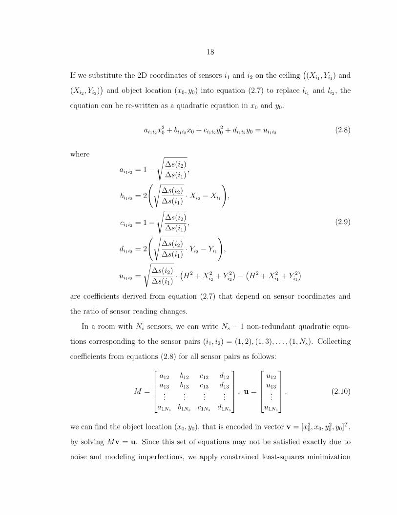
18
If we substitute the 2D coordinates of sensors i1 and i2 on the ceiling((Xi1 , Yi1) and
(Xi2 , Yi2))
and object location (x0, y0) into equation (2.7) to replace li1 and li2 , the
equation can be re-written as a quadratic equation in x0 and y0:
ai1i2x20 + bi1i2x0 + ci1i2y
20 + di1i2y0 = ui1i2 (2.8)
where
ai1i2 = 1−
√∆s(i2)
∆s(i1),
bi1i2 = 2
(√∆s(i2)
∆s(i1)·Xi2 −Xi1
),
ci1i2 = 1−
√∆s(i2)
∆s(i1),
di1i2 = 2
(√∆s(i2)
∆s(i1)· Yi2 − Yi1
),
ui1i2 =
√∆s(i2)
∆s(i1)·(H2 +X2
i2+ Y 2
i2
)−(H2 +X2
i1+ Y 2
i1
)
(2.9)
are coefficients derived from equation (2.7) that depend on sensor coordinates and
the ratio of sensor reading changes.
In a room with Ns sensors, we can write Ns − 1 non-redundant quadratic equa-
tions corresponding to the sensor pairs (i1, i2) = (1, 2), (1, 3), . . . , (1, Ns). Collecting
coefficients from equations (2.8) for all sensor pairs as follows:
M =
a12 b12 c12 d12
a13 b13 c13 d13...
......
...a1Ns b1Ns c1Ns d1Ns
, u =
u12
u13...
u1Ns
. (2.10)
we can find the object location (x0, y0), that is encoded in vector v = [x20, x0, y
20, y0]T ,
by solving Mv = u. Since this set of equations may not be satisfied exactly due to
noise and modeling imperfections, we apply constrained least-squares minimization

19
to find v as follows:
v∗ = arg minv‖Mv − u‖2
l2
s.t. v ≥ 0,v ≤ [W 2,W, L2, L]T .
(2.11)
The 2-nd and 4-th entries of the solution vector, provide an estimate of the object
location (x0, y0). The cost function is strictly convex and has unique global minimum
when matrix M has full column rank (Ns ≥ 5). The pseudo-code for this algorithm
appears in Algorithm 1.
Algorithm 1: Localization via Passive Illumination
Input : Vectors of sensor readings: s0 for empty room and s for occupied
room, room dimensions W , L and H, sensor coordinates (xi, yi, H)
for i = 1, . . . , Ns
Output: Estimated location (x0, y0)
1 Let ∆s← s− s0;
2 Calculate coefficients ai1i2 , bi1i2 , ci1i2 , di1i2 , ui1i2 for
(i1, i2) = (1, 2), (1, 3), . . . , (1, Ns) in (2.8);
3 Construct matrix M and vector u as in (2.10);
4 Use quadratic programming to find the optimal solution v∗ to minimization
(2.11);
5 Estimated location: (x0, y0)← (v∗2, v∗4).
2.3 Experiments
We have tested the performance of our passive-illumination-based localization algo-
rithm in both simulated and real-world experiments. We performed simulations in
MATLAB and Unity3D, a video game development environment. For our real-world ex-
periments, we have built a small-scale testbed using a network of synchronized small
LED light sources and single-pixel color sensors. We tested our algorithm in the
ideal case, under illumination change between the empty and occupied room states,

20
and also in the presence of noise in sensor readings. Detailed information about our
experimental setup, testbed, and results can be found on our project’s web page1.
2.3.1 Experimental setup
We built a testbed room with size W=122.5cm, L=223.8cm and H=70.5cm and
9 identical source-sensor modules placed on the ceiling on a 3 × 3 grid (Fig. 2·3).
In simulation experiments, the room size and source/sensor locations are set to be
identical to our testbed. Each module contains an LED light source and a single-
pixel light sensor. The light sources will be modulated in experiments with active
illumination algorithms, as we will see in the next chapter. For passive illumination,
we simply turned on all light sources at their maximum intensity and kept them
unchanged to produce constant light.
0 50 100 150 200x (cm)
0
20
40
60
80
100
120
y (
cm
)
SourcesSensors
Figure 2·3: Layout of source-sensor modules on the ceiling.
We used flat (negligible height) rectangular objects of 6 different sizes (Table 2.1).
Our object size choices are quite realistic at room-scale. For example, if we scale the
1http://vip.bu.edu/projects/vsns/privacy-smartroom/active-illumination/

21
testbed area 8-fold to a room of dimensions about 3.5×6m, then our smallest object
(1x) will be about the size of a small plate (14cm diameter) and our largest object
(64x) will be about the size of a table (70×140cm). We placed the objects on the
floor so that their sides are parallel to those of the room.
Table 2.1: Dimensions of rectangular objects used in experiments.
Relative Size Width (cm) Length (cm)64x 25.8 51.132x 25.8 25.516x 12.9 26.08x 12.9 13.04x 6.4 12.91x 3.2 6.4
2.3.2 Simulation Experiments
To validate our active and passive illumination algorithms, we simulated the room
with light sources and sensors in both MATLAB and Unity3D, a game development
environment that can simulate realistic scenes.
In MATLAB simulation, we generated the floor albedo maps α(x, y) for empty and
occupied states, and then calculated the sensor readings in each state using equations
(2.1), (2.2) and (2.3). The MATLAB simulations are idealized since the sensor readings
match the light reflection model perfectly with no inconsistencies.
In Unity3D simulation, we simulated the LED light sources using Unity3D’s built-
in point light source. However, the built-in point light source is omnidirectional and
does not support a light intensity distribution function q(·). Therefore, we placed a
spherical cover around each light source. The cover is semi-transparent and blocks
parts of the light from the source. We set the transparency of the cover at different
angles differently in order to match the q(·) function. To simulate a light sensor, we
placed Unity3D’s virtual camera on the ceiling looking downward. The sensor reading

22
(a) Simulation of a light source
with object placed on the floor
(b) Top view of the scene
Figure 2·4: Illustration of a Unity3D scene used in experiments.
is a weighted average of the camera’s pixel values, where the weight is each pixel’s
solid angle to the center of the camera lens. To simulate sunlight (as part of ambient
illumination), we used a directional light source which produces parallel rays.
An illustration of a Unity3D scene of the room is shown in Fig. 2·4. The Unity3D
model is only used to collect data while the localization algorithms are implemented
in MATLAB.
In both MATLAB and Unity3D, we uniformly set the albedo of the floor to 0.5
and of the object to 0. We placed the center of the object at 20 different locations
equally-spaced on a 5× 4 grid (Fig. 2·5). We evaluated our algorithm’s performance
in terms of localization error defined as the Euclidean distance between the true
and estimated locations. First, we evaluated the performance of our algorithm for
different object sizes, in both simulation environments, without noise. The mean and
standard deviation of the localization errors with respect to the object size are shown
in Fig. 2·6. We note that our passive illumination algorithm works better for smaller
objects, which is consistent with the negligible object size assumption (assumption 2
in Section 2.2) used to derive this algorithm.
We also tested the robustness of our passive illumination algorithm under illumi-

23
0 50 100 150 200x (cm)
0
20
40
60
80
100
120
y (c
m)
Object center positions
Figure 2·5: 20 locations on the floor where we placed the center ofthe objects.
nation change in Unity3D. An illumination change refers to the change of ambient
light level b(i) (Eq. 2.3) between the empty and occupied room states. We performed
tests using the 64x object, and turned on/off the simulated sun light to mimic day
and night. The results are shown in Fig. 2·7. When there is an illumination change,
the performance of the algorithm gets significantly worse. This was to be expected
since the passive illumination algorithm assumes that the only change in the sensor
readings is caused by the object; it cannot handle illumination changes.
Furthermore, we tested the effect of sensor noise on the performance of our algo-
rithms. We assumed that the noise corrupting each sensor reading is an independent
and identically-distributed, zero-mean Gaussian. In MATLAB simulation, we added
noise to all sensor readings in both the empty and occupied room states. We used the
16x object, and we varied the standard deviation of noise from 10−4 to 10−3 in 10−4
increments. (10−3 represents about 6.84% of the maximum change in any sensor’s
reading between empty and occupied room states.) Fig. 2·8 shows the mean and stan-

24
1 4 8 16 32 64Relative object size
0
1
2
3
4
5
6
Ave
rage
loca
lizat
ion
erro
r (c
m)
MATLAB simulationUnity3D simulation
Figure 2·6: Mean and standard deviation of localization errors of ourpassive illumination algorithm with respect to the relative object sizein both MATLAB and Unity3D simulations. The dots represent averagelocalization errors, while the bars indicate the standard deviation oferrors for each object size.
dard deviation of localization errors for passive and active illumination algorithms as
a function of the standard deviation of noise. Although the magnitude of noise is
small compared with that of the signal (sensor reading changes between empty and
occupied states), the average localization error increases and saturates quickly as the
noise level increases, which suggests that the passive illumination algorithm is very
sensitive to noise. This is because the equation (2.6) is based on the ratio of sensor
reading changes and therefore the noise will be magnified.

25
Bright->Bright Dark->Dark Bright->Dark Dark->Bright0
10
20
30
40
50
60
70
80
90
100
Ave
rage
loca
lizat
ion
erro
r (c
m)
Figure 2·7: Mean and standard deviation of localization errors of thepassive illumination algorithm for all lighting combinations in Unity3Dsimulation (empty room → occupied room).
0 1 2 3 4 5 6 7 8 9 10Standard deviation of Gaussian noise 10-4
0
10
20
30
40
50
60
70
80
Ave
rage
loca
lizat
ion
erro
r (c
m)
Figure 2·8: Mean and standard deviation of localization errors of ourpassive illumination algorithm with respect to the standard deviation ofGaussian noise in MATLAB simulation. The mean and standard deviationof errors at each noise level are calculated by combining results from 3repetitions of the experiment.

26
2.3.3 Testbed Experiments
To test our approach in a real-world setting, we built a room mock-up using a white
rectangular foam board as the floor and a 3×3 array of ceiling-mounted light source-
sensor modules. Each module consists of a Particle Photon board controlling an
LED and a single-pixel light sensor. We estimated the q(·) function following the
process described in Fig. 2·2. We note that the sensors have no lens and measure
photon flux not radiance. A photo of our testbed is shown in Fig. 2·9. This is a
small-scale proof-of-concept testbed to quantitatively validate the feasibility of active-
illumination based indoor localization. Although idealized (no walls/furniture, floor
and objects have uniform albedo), it is a much-needed first step before developing a
full-scale smart-room testbed. While this is not an accurate representation of complex
real-world scenarios, it does capture real-world non-idealities such as sensor noise,
non-Lambertian surfaces, indirect light, and fluorescent light flicker and provides
insights into the localization accuracy relative to testbed dimensions.
During data collection, the LEDs turn on all 4 channels (red, green, blue and
white) at maximum intensity and the single-pixel sensors record readings from the
white channel only (red, green and blue channel readings are ignored). When a sensor
records, it takes 4 consecutive readings which are then averaged together to reduce
noise. This process yields 9 noise-reduced sensor readings in the passive illumination
case.
Similar to the simulation experiments, we tested our algorithm in the testbed for
different object sizes (from 8x to 64x) at all 20 locations. We did not use the 1x
and 4x objects because their sensor reading changes are too small and get buried in
noise. We recorded data in a completely dark room with no ambient illumination
(fluorescent lights off).
As shown in Fig. 2·10, the performance of our passive illumination algorithm gets
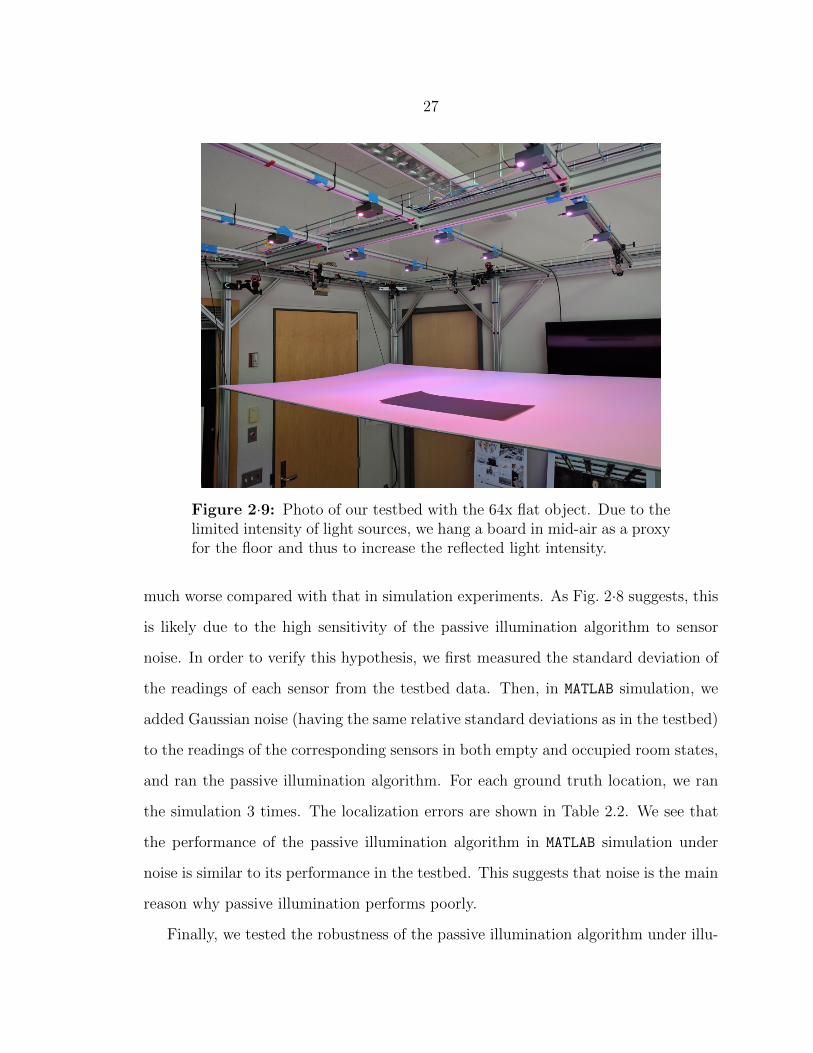
27
Figure 2·9: Photo of our testbed with the 64x flat object. Due to thelimited intensity of light sources, we hang a board in mid-air as a proxyfor the floor and thus to increase the reflected light intensity.
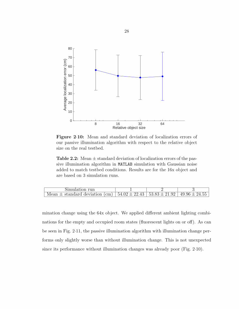
much worse compared with that in simulation experiments. As Fig. 2·8 suggests, this
is likely due to the high sensitivity of the passive illumination algorithm to sensor
noise. In order to verify this hypothesis, we first measured the standard deviation of
the readings of each sensor from the testbed data. Then, in MATLAB simulation, we
added Gaussian noise (having the same relative standard deviations as in the testbed)
to the readings of the corresponding sensors in both empty and occupied room states,
and ran the passive illumination algorithm. For each ground truth location, we ran
the simulation 3 times. The localization errors are shown in Table 2.2. We see that
the performance of the passive illumination algorithm in MATLAB simulation under
noise is similar to its performance in the testbed. This suggests that noise is the main
reason why passive illumination performs poorly.
Finally, we tested the robustness of the passive illumination algorithm under illu-
28
8 16 32 64Relative object size
0
10
20
30
40
50
60
70
80
Ave
rage
loca
lizat
ion
erro
r (c
m)
Figure 2·10: Mean and standard deviation of localization errors ofour passive illumination algorithm with respect to the relative objectsize on the real testbed.
Table 2.2: Mean ± standard deviation of localization errors of the pas-sive illumination algorithm in MATLAB simulation with Gaussian noiseadded to match testbed conditions. Results are for the 16x object andare based on 3 simulation runs.
Simulation run 1 2 3Mean ± standard deviation (cm) 54.02± 22.43 53.83± 21.92 49.96± 24.55
mination change using the 64x object. We applied different ambient lighting combi-
nations for the empty and occupied room states (fluorescent lights on or off). As can
be seen in Fig. 2·11, the passive illumination algorithm with illumination change per-
forms only slightly worse than without illumination change. This is not unexpected
since its performance without illumination changes was already poor (Fig. 2·10).

29
Bright->Bright Dark->Dark Bright->Dark Dark->Bright0
10
20
30
40
50
60
70
80
Ave
rage
loca
lizat
ion
erro
r (c
m)
Figure 2·11: Mean and standard deviation of localization errors ofthe passive illumination algorithm for all lighting combinations on thereal testbed (empty room → occupied room). Results are for the 64xobject.
2.4 Summary
In this chapter, we proposed a localization algorithm via passive illumination. Our
passive illumination algorithm can localize a flat object accurately in idealized sim-
ulations in MATLAB and Unity3D (average localization error ≤ 4cm on a floor of size
122.5cm×223.8cm), but it is very sensitive to sensor reading noise and ambient illu-
mination changes. It also has poor performance on the real testbed due to real-world
non-idealities. This is expected since it assumes that the sensor reading changes are
only due to object presence.

30
Chapter 3
Model-based indoor localization via active
scene illumination
In this chapter, we will introduce our proposed model-based localization algorithms
via active illumination. With the use of an array of modulated LED light sources,
our active illumination algorithms are supposed to be more robust to noise and illu-
mination change than the passive illumination algorithm developed in Chapter 2.
3.1 Active illumination methodology
Fig. 3·1 provides an overview of the active illumination methodology. Compared with
a passive illumination system using constant light sources, our active illumination
system modulates the light sources and measures responses from single-pixel sensors.
The sensor responses are results of 1) light modulation pattern, 2) ambient light
intensity and noise, and 3) shapes, locations and surface properties of all objects in
the room. Ambient light intensity may vary, but since light sources can be modulated,
we can easily measure and eliminate the contribution of ambient light. Therefore, the
relationship between light modulation and sensor responses is purely determined by
the room state. The localization algorithm will then compute the difference of current
room state from a background (e.g., empty room) and estimate the location of the
object that causes the change.

31
Figure 3·1: Illustration of the active illumination methodology.
Consider light source with index j and sensor with index i. Define
A(i, j) =
W∫0
L∫0
ImaxSq(βj) cos βj cos2 θi α(x, y)
16π2Dj2(H2 + li
2)dxdy (3.1)
where βj, Dj, θi and li are functions of x and y and are shown in Fig. 2·1. If we
substitute Eq. (2.1), Eq. (2.2) and Eq. (3.1) into Eq. (2.3), we get
s(i) = b(i) +
Nf∑j=1
f(j)A(i, j) (3.2)
where f(j) is the relative intensity of light source j scaled to range [0, 1]. Eq. (3.2)
implies that sensor i’s reading is the sum of contributions of all light sources and
ambient light. The meaning of A(i, j) is the contribution of source j to the reading
of sensor i per unit light intensity. It is clear from equation (3.1) that A(i, j) is
determined by room geometry, material properties and source and sensor locations,

32
but it is not affected by ambient light. Suppose we have Nf light sources and Ns
sensors. Then, we can rewrite Eq. (3.2) in matrix form:
s = Af + b (3.3)
where s is an Ns× 1 vector of sensor readings, f is an Nf × 1 vector of relative source
intensities, and b a vector of ambient light levels at each sensor. A is an Ns × Nf
matrix whose ij-th entry is A(i, j) in Eq.(3.1). We call matrix A the light transport
matrix.
We further relate A(i, j) to floor reflectivity (albedo). Let
C(i, j;x, y) =ImaxSq(βj) cos βj cos2 θi
16π2Dj2(H2 + li
2)(3.4)
then
A(i, j) =
W∫0
L∫0
C(i, j;x, y)α(x, y) dxdy. (3.5)
The meaning of C(i, j;x, y) is the light contribution of source j to the reading of sensor
i via floor location (x, y) with unit light source intensity and unit floor albedo. It can
be seen from Eq. (3.4) that C(i, j;x, y) is a function of room height, light intensity
distribution function q(·), locations of source j and sensor i, and floor position (x, y).
It is completely determined by the characteristics of room, light sources and sensors,
and once we have this information, we can calculate C(i, j;x, y) without modulating
sources and measuring with sensors.
Suppose we have obtained light transport matrices for two room states: A0 when
the room is empty, and A when an object is placed somewhere in the room. Taking

33
the difference between the ij-th entries of the two light transport matrices, we get:
∆A(i, j) = A(i, j)− A0(i, j) =
W∫0
L∫0
C(i, j;x, y)∆α(x, y) dxdy (3.6)
where ∆α(x, y) is the change of floor albedo between the two states at position (x, y).
Albedo change is usually the result of object appearance, and in the case of a single
object, it should be concentrated in one connected blob. If we discretize the floor
plane into a grid with spacing δ, we can re-write the discretized approximation to
Eq. (3.6) in matrix and vector form as follows:
∆A = δ2C∆α (3.7)
where vector ∆A contains lexicographically-scanned elements of matrix ∆A, ∆α is a
vector of albedo changes at all locations (x, y) on the discretized floor grid, and C is a
matrix of C(i, j;x, y) values, whose rows correspond to source-sensor pairs (i, j) and
columns correspond to positions (x, y). We call matrix C the light contribution
matrix. The length of vector ∆α (i.e. the number of columns of matrix C) is
determined by the discretization stepsize δ, and in our experiments, ∆α has length
of bWδc × bL
δc.
The light contribution matrix C can be calculated up to a constant factor given
room dimensions, light source and sensor locations and light intensity distribution
function q(·) (Fig. 2·2). The light transport matrices A for empty and occupied room
states can be obtained from two sets of sensor measurements in corresponding room
states, which we will discuss in the next section. The goal is to estimate the albedo
change map on the floor (vector ∆α) and then estimate the object location. In
Section 3.3, we will propose two variants of localization algorithm based on based on
this active illumination methodology. Both variants follow the assumptions of the
light reflection model, as stated in Section 2.1.

34
3.2 Obtaining light transport matrix A
The light transport matrix A can be estimated via light source modulation. In an
active illumination system, we can specify the intensity f(j) of any light source j to
any value in range [0, 1].
Suppose we have specified the intensities of all light sources as a vector f0 (base
light). Then, by Eq. (3.3), we can obtain a vector of sensor readings under base light
s0 = Af0 + b. Assume that the contribution of ambient light b remains constant
during the light modulation process. If we add some perturbation ∆f to the base
light f0, the sensor reading will become s = A(f0 + ∆f) + b. Taking the difference of
the two sets of sensor readings, we get
∆s = s− s0 = A∆f (3.8)
so that the contribution of ambient light b is eliminated.
To obtain the matrix A, we need to design a set of perturbations that form a basis.
Therefore, we need a base light vector and n perturbations at times t1, t2, . . . , tn where
n ≥ Nf . Let matrix ∆F = [∆f(t1),∆f(t2), . . . ,∆f(tn)] and the corresponding sensor
reading changes ∆S = [∆s(t1),∆s(t2), . . . ,∆s(tn)]. Then, by Eq. (3.8), we have
∆S = A∆F (3.9)
and
∆S∆FT = A∆F∆FT. (3.10)
We can estimate A by multiplying (∆F∆FT)−1 on both sides:
A = ∆S∆FT(∆F∆FT)−1. (3.11)

35
For convenience, we call a light intensity vector f with specified values a light
state, and call a set of light states (including base light vector and base light + all
perturbations) a light pattern. In our experiments, we use a light pattern where
the base light is all-zero and each perturbation is a one-hot vector (one light source
on at maximum intensity). Therefore, our light pattern has Nf + 1 light states.
Although constant ambient illumination is not an assumption of localization via
active illumination, it does assume that the ambient light should stay constant during
modulation through the entire light pattern so that its contribution can be eliminated.
This assumption is easy to satisfy for gradually-changing ambient light sources (e.g.,
sunlight) since the modulation-response time is short; however, ambient light sources
that flicker (e.g., fluorescent light) or a sudden change of ambient illumination (e.g.,
turning on/off an ambient light source) will violate this assumption and bring noise
into the estimated light transport matrix. Another problem with light modulation is
that the modulation process itself will produce visible flickers to human eyes, causing
discomfort, if the modulation frequency of a light source is below 60Hz. The solution
to both issues is to increase the light modulation frequency; however, the modulation
frequency is limited by the minimum integration time needed for a sensor to get a
stable reading. We will ignore these issues in this dissertation, since we are presenting
a proof-of-concept study rather than a commercial product.
3.3 Localization via active illumination
In this section, we will introduce our proposed localization algorithm via active illu-
mination. Given light transport matrices A0 for empty room, A for occupied room
and light contribution matrix C, our algorithm will estimate the change of albedo
∆α and then estimate the location of the object. We will propose two variants of the
algorithm using different penalty functions.

36
3.3.1 LASSO algorithm
Eq. (3.7) is usually an underdetermined system; the number of unknowns (number
of points on the discretized floor grid) is usually larger than the number of equations
(number of light source-sensor pairs). Therefore, the solution to ∆α is not unique. To
obtain an accurate estimate of ∆α which is close to the ground truth, an additional
constraint is required.
Since object size is usually small compared to room size, we can start by assuming
that ∆α is a sparse vector. Inspired by LASSO regression, we add the l1-norm on ∆α
to the error function to promote sparsity and solve the following convex optimization
problem:
∆α∗ = arg min∆α
[∥∥∆A− δ2C∆α∥∥2
l2+ λδ2 ‖∆α‖l1
](3.12)
where λ is the weight of the l1 penalty term. Given the value of λ, the problem (3.12)
can be solved with a gradient descent optimization algorithm. In our experiments we
used the CVX package, a MATLAB toolkit for convex programming1. A larger λ will
promote the solution ∆α∗ to have fewer non-zero entries, and vice versa. The value
of λ can be optimized using a grid search, where the best λ will minimize the average
localization error.
After estimating the albedo change ∆α∗, the location of the object that causes
the albedo change is estimated as the centroid of the magnitude of ∆α∗:
x0 =
∑x,y x · |∆α∗(x, y)|∑x,y |∆α∗(x, y)|
,
y0 =
∑x,y y · |∆α∗(x, y)|∑x,y |∆α∗(x, y)|
.
(3.13)
Estimating object location using centroid of albedo change is accurate under the
assumption that albedo change is uniform within the object area. This assumption
1http://cvxr.com/cvx/

37
is easily satisfied if both the floor and the object have a uniform albedo. When the
texture of the floor or the object gets complicated (e.g., floor with colorful tiles), this
estimation will introduce errors, but the estimated object location will likely still stay
within the object area if the albedo change estimation is accurate enough.
The pseudo-code for this algorithm is shown in Algorithm 2.
Algorithm 2: Localization via Active Illumination - LASSO AlgorithmInput : Light transport matrices: A0 for empty room and A for occupied room,
room dimensions W , L and H, all light source and sensor coordinates
Output: Estimated location (x0, y0)
1 Calculate light contribution matrix C where C(i, j;x, y) = const · q(βj) cosβj cos2 θiD2
j ·(H2+l2i )for
i ∈ 1, . . . , Ns, j ∈ 1, . . . , Nf, x ∈ [0, L], y ∈ [0,W ] with spacing δ;
2 Let ∆A be a vector form of ∆A = A−A0;
3 Calculate the optimal solution ∆α∗ for problem (3.12) without constraints;
4 Estimated location: (x0, y0)← centroid of |∆α∗|.
3.3.2 Localized ridge regression algorithm
The l1 penalty term in the LASSO algorithm (Algorithm 2) tends to create spikes
in the resulting albedo change map ∆α (Fig. 3·3 (a)(c)). This might be a good
estimation for small objects, but for larger objects this estimated map will become
too sparse. Therefore, we propose another version of the active illumination algorithm
using the squared l2 norm of ∆α as the penalty term, similar to ridge regression. The
optimization problem becomes as follows:
∆α∗0 = arg min∆α
[∥∥∆A− δ2C∆α∥∥2
l2+ σδ2 ‖∆α‖2
l2
]. (3.14)
The squared l2 penalty term penalizes large entries in ∆α, and therefore helps
generate a more smooth albedo change map. σ is a weight of the l2 penalty term
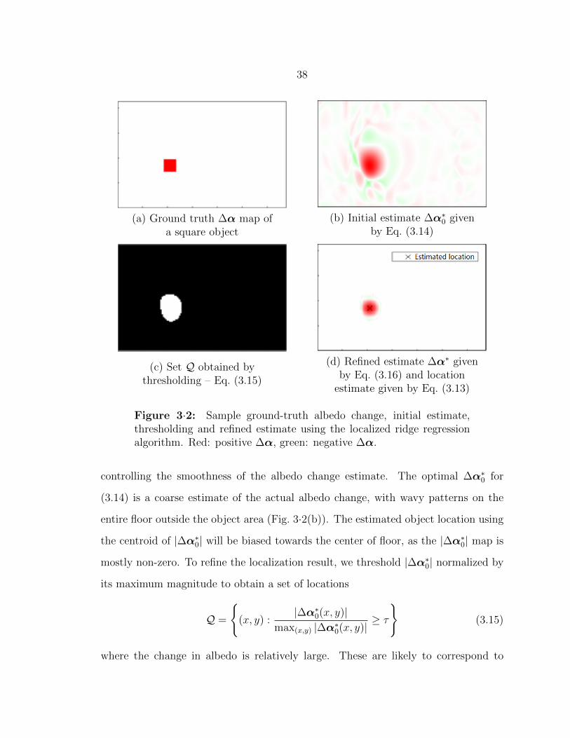
38
(a) Ground truth ∆α map ofa square object
(b) Initial estimate ∆α∗0 givenby Eq. (3.14)
(c) Set Q obtained bythresholding – Eq. (3.15)
(d) Refined estimate ∆α∗ givenby Eq. (3.16) and location
estimate given by Eq. (3.13)
Figure 3·2: Sample ground-truth albedo change, initial estimate,thresholding and refined estimate using the localized ridge regressionalgorithm. Red: positive ∆α, green: negative ∆α.
controlling the smoothness of the albedo change estimate. The optimal ∆α∗0 for
(3.14) is a coarse estimate of the actual albedo change, with wavy patterns on the
entire floor outside the object area (Fig. 3·2(b)). The estimated object location using
the centroid of |∆α∗0| will be biased towards the center of floor, as the |∆α∗0| map is
mostly non-zero. To refine the localization result, we threshold |∆α∗0| normalized by
its maximum magnitude to obtain a set of locations
Q =
(x, y) :
|∆α∗0(x, y)|max(x,y) |∆α∗0(x, y)|
≥ τ
(3.15)
where the change in albedo is relatively large. These are likely to correspond to

39
the area where the object appeared. Then, in the second step, we solve the ridge
regression problem again, but the solution is now restricted to a subset of locations
in Q.
∆α∗ = arg min∆α
[∥∥∆A− δ2C∆α∥∥2
l2+ σδ2 ‖∆α‖2
l2
]s.t. ∆α(x, y) = 0, ∀(x, y) 6∈ Q
(3.16)
After obtaining the optimal ∆α∗ from (3.16), we use the centroid of the |∆α∗|
map as the estimated object location (Eq. (3.13)).
Both optimization problems (3.14) and (3.16) are convex and so have a closed-
form solution, which we derive in Appendix A. σ and τ are two parameters that affect
the algorithm’s performance, and we use grid search to find the best set of parameters
yielding the minimum average localization error.
The pseudo-code for this algorithm appears in Algorithm 3 below. Fig. 3·2 shows
a sample ground truth albedo change map and the results of each step in the localized
ridge regression algorithm.
Algorithm 3: Localization via Active Illumination - Localized Ridge Regression
AlgorithmInput : Light transport matrices: A0 for empty room and A for occupied room,
room dimensions W , L and H, all light source and sensor coordinates
Output: Estimated location (x0, y0)
1 Calculate light contribution matrix C where C(i, j;x, y) = const · q(βj) cosβj cos2 θiD2
j ·(H2+l2i )for
i ∈ 1, . . . , Ns, j ∈ 1, . . . , Nf, x ∈ [0, L], y ∈ [0,W ] with spacing δ;
2 Let ∆A be a vector form of ∆A = A−A0;
3 Calculate the optimal solution ∆α∗0 for problem (3.14) without constraints;
4 Threshold |∆α∗0| using τ to get the point set Q;
5 Calculate the optimal solution ∆α∗ for problem (3.16) with ∆α constrained inside
Q;
6 Estimated location: (x0, y0)← centroid of |∆α∗|.

40
3.3.3 Comparison of LASSO and Localized ridge regression algorithms
To compare the performance of the two active illumination algorithm variants on
objects of different sizes, we did simulation experiments in MATLAB. The room size,
light source and sensor locations and object sizes used are the same as those described
in Section 2.3.1. We put each object at the 20 locations marked in Fig. 2·5, and
compared the two algorithm variants in terms of estimated albedo change map and
localization error. The parameters (λ for LASSO algorithm and σ and τ for localized
ridge regression algorithm) are optimized for each object size to minimize the average
localization error.
Fig. 3·3 shows sample albedo change and location estimates of both algorithm
variants for 4x and 64x objects. It is seen from Fig. 3·3 that the LASSO algorithm
gives higher localization errors since it tends to choose only a few representative
columns of matrix C whose weighted sum is close to ∆A. The locations corresponding
to these columns can be away from the object center. The localized ridge regression
algorithm, on the other hand, tends to choose columns of matrix C inside a blob, and
therefore gives a better estimate of the location and size of the object.
We then computed the mean and standard deviation of localization errors of both
algorithm variants for all object sizes, which are shown in Fig. 3·4. The localization
errors of the localized ridge regression algorithm are an order of magnitude smaller
than those for the LASSO algorithm. Since the localized ridge regression algorithm
outperforms the LASSO algorithm in all scenarios, we advocate the use of localized
ridge regression algorithm and explore it in more detail in the following sections.
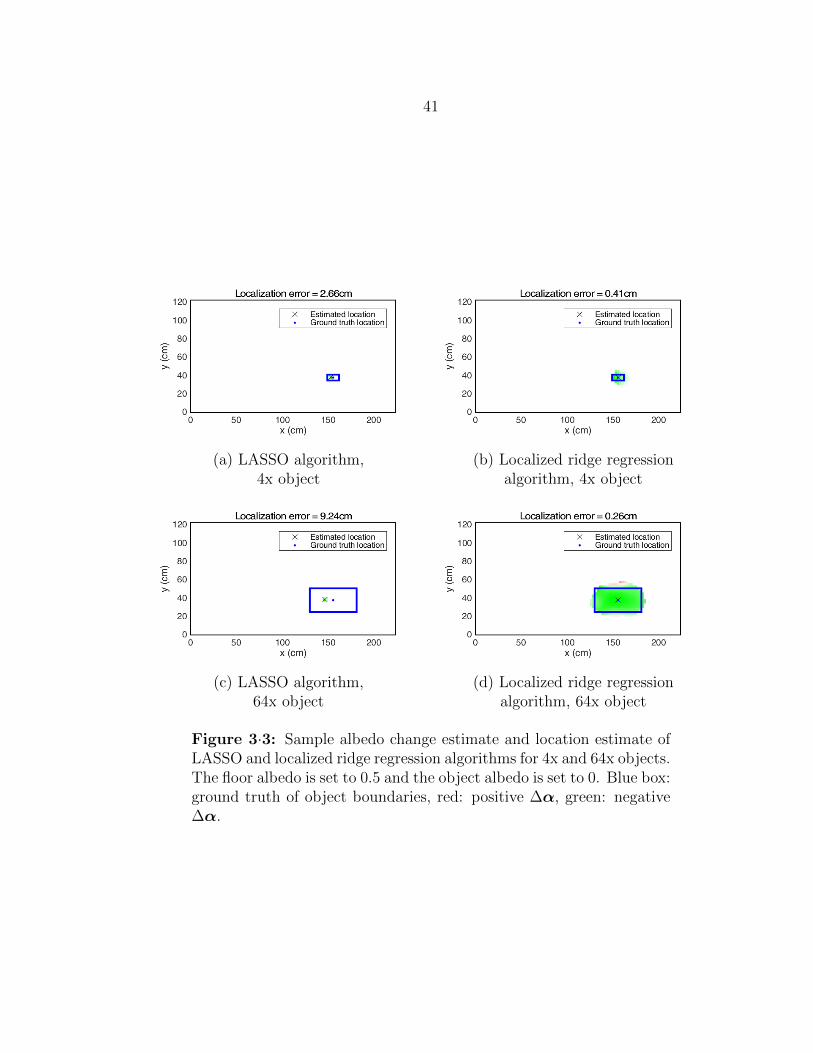
41
(a) LASSO algorithm,4x object
(b) Localized ridge regressionalgorithm, 4x object
(c) LASSO algorithm,64x object
(d) Localized ridge regressionalgorithm, 64x object
Figure 3·3: Sample albedo change estimate and location estimate ofLASSO and localized ridge regression algorithms for 4x and 64x objects.The floor albedo is set to 0.5 and the object albedo is set to 0. Blue box:ground truth of object boundaries, red: positive ∆α, green: negative∆α.

42
1 4 8 16 32 64Relative object size
0
2
4
6
8
10
12
14
16
Avera
ge localiz
ation e
rror
(cm
)
LASSO algorithmLocalized ridge regression algorithm
Figure 3·4: Mean and standard deviation of localization errors of theLASSO and localized ridge regression algorithms with respect to therelative object size in MATLAB simulation.

43
3.4 Comparison with localization via passive illumination
In Section 2.3 we demonstrated via simulation and testbed experiments that the
passive illumination algorithm is accurate in ideal cases but sensitive to sensor noise
and illumination changes. In this section, we will validate the accuracy and robustness
of our active illumination algorithm via the same sets of experiments and compare it
with the passive illumination algorithm.
3.4.1 Simulation and testbed experiments
We first validated our active illumination algorithm (localized ridge regression) in
MATLAB and Unity3D simulations in ideal case, with no noise or illumination changes.
The room size, light source and sensor locations, object sizes and other experiment
settings follow the experiments described in Section 2.3.2, except that the light sources
are now modulated. In MATLAB simulations, we first generated the ground truth albedo
change map ∆α given object size and location, and then calculated the change of
light transport matrix ∆A using Eq. (3.7). In Unity3D simulations, we modulated
the light sources with animation scripts, using the light pattern described in Section
3.2 to obtain the light transport matrices for empty and occupied room states, and
then took the difference between the two to obtain ∆A. The light contribution matrix
C is pre-computed and used in both types of simulations. We put each object at the
20 locations marked in Fig. 2·5. For each object size and simulation environment, we
optimized the parameters σ and τ to minimize the average localization error.
Fig. 3·5 shows the mean and standard deviation of localization errors of passive
and active illumination algorithms in both simulations. Unlike passive illumination,
our active illumination algorithm favors larger object sizes, although its performance
is slightly worse than that for the passive illumination algorithm for smaller objects.
The MATLAB and Unity3D simulation results exhibit similar trends.

44
We then tested both algorithms’ robustness to illumination changes and sensor
noise in Unity3D and MATLAB simulations respectively, following the same procedure
as described in Section 2.3.2. The localization errors for all ambient illumination
scenarios are shown in Fig. 3·6 (a). The active illumination algorithm performs con-
sistently well even when there is an illumination change between empty and occupied
room states, which is expected. Fig. 3·6 (b) shows the localization errors versus the
standard deviation of Gaussian noise in sensor readings. The active illumination al-
gorithm is much more robust to noise, whose average localization error is almost an
order of magnitude smaller than that of passive illumination as noise level increases.
Lastly, we validated our active illumination algorithm on the real testbed (Fig. 2·9).
We collected data under the same lighting condition as when we tested the passive
illumination algorithm (fluorescent light off). For empty room state, we ran the light
modulation process for several cycles through the light pattern, and averaged the
obtained light transport matrices to obtain A0. Then, for each object size from 8x
to 64x, we put the object at all 20 locations and collected one light transport matrix
A per location. Localization errors with respect to object size are shown in Fig. 3·7
(a). We also tested the algorithms’ robustness to illumination changes by switching
the fluorescent light in the room, and the results are shown in Fig. 3·7 (b). The
active illumination algorithm performs well for all object sizes and under illumina-
tion changes on the testbed, which is consistent with the simulation results. Due to
flicker in the fluorescent light, the active illumination algorithm has higher standard
deviations of errors when the occupied room state is bright.

45
1 4 8 16 32 64Relative object size
0
1
2
3
4
5
6
Ave
rag
e lo
ca
liza
tio
n e
rro
r (c
m)
Passive illuminationActive illumination (localized ridge regression)
(a) MATLAB simulations
1 4 8 16 32 64Relative object size
0
1
2
3
4
5
6
Ave
rag
e lo
ca
liza
tio
n e
rro
r (c
m)
Passive illuminationActive illumination (localized ridge regression)
(b) Unity3D simulations
Figure 3·5: Mean and standard deviation of localization errors ofpassive and active illumination algorithms with respect to the relativeobject size in MATLAB and Unity3D simulations.

46
Bright->Bright Dark->Dark Bright->Dark Dark->Bright0
10
20
30
40
50
60
70
80
90
100
Ave
rag
e lo
ca
liza
tio
n e
rro
r (c
m)
Passive illuminationActive illumination
(a) Localization errors under different ambient illuminationscenarios in Unity3D simulation (empty room → occupied room).
0 1 2 3 4 5 6 7 8 9 10Standard deviation of Gaussian noise 10
-4
0
10
20
30
40
50
60
70
80
Ave
rag
e lo
ca
liza
tio
n e
rro
r (c
m)
Passive illuminationActive illumination
(b) Localization errors with respect to standard deviation ofGaussian noise in MATLAB simulation. Mean and standard deviation
of errors at each noise level are calculated by combining resultsfrom 3 repetitions of the experiment.
Figure 3·6: Mean and standard deviation of localization errors ofpassive and active illumination algorithms under different ambient il-lumination scenarios and noise levels.

47
8 16 32 64Relative object size
0
10
20
30
40
50
60
70
80
Ave
rag
e lo
ca
liza
tio
n e
rro
r (c
m)
Passive illuminationActive illumination
(a) Localization errors with respect to object size.
Bright->Bright Dark->Dark Bright->Dark Dark->Bright0
10
20
30
40
50
60
70
80
Ave
rag
e lo
ca
liza
tio
n e
rro
r (c
m)
Passive illuminationActive illumination
(b) Localization errors under different ambient illuminationscenarios (empty room → occupied room). The 64x object is used.
Figure 3·7: Mean and standard deviation of localization errors ofpassive and active illumination algorithms with respect to object sizeand under different ambient illumination scenarios on the real testbed.
48
3.4.2 Discussion
Effect of object size: As suggested by Fig. 3·5, the active illumination algorithm
performs better for larger objects but slightly worse for smaller ones. This is because
the l2 penalty term in the cost function smooths the ∆α map and therefore favors
large objects. On the contrary, the passive illumination algorithm performs better
for smaller objects since the algorithm assumes that the object size is negligible
compared to the floor size, but its performance becomes significantly worse when the
object gets large. Since we are considering large objects (e.g., humans in an office
room) in general, the active illumination algorithm would be more useful in practice.
Effect of illumination change: The experimental results in Fig. 3·6 (a) and
Fig. 3·7 (b) suggest that the active illumination algorithm is robust under illumina-
tion change while the passive illumination algorithm is not. This is consistent with
the assumptions used to derive each algorithm. The passive illumination algorithm
assumes that the change in the sensor reading is only due to the arrival of an object
and does not account for the possibility of illumination change between the empty
and occupied room states. The active illumination algorithm, however, only needs to
compute the change in the light transport matrix between the empty and occupied
room states. The light transport matrix is determined by room geometry, sensor and
source placements and floor albedo distribution, and is unaffected by ambient light.
The estimation of a light transport matrix too is unaffected by ambient light since
it is based on measuring the change in sensor readings due to light modulation. The
only crucial assumption needed for this to succeed is that the ambient light remains
constant during the process of measuring a single light transport matrix, as discussed
in Section 3.2.
Effect of noise: Experimental results in simulations (Fig. 3·6 (b)) and the real
testbed (Fig. 3·7 (a)) suggest that the passive illumination algorithm is more sensitive
49
to noise than the active illumination algorithm. In passive illumination, Eq. (2.6) is
based on the ratio of changes in the sensor readings. The sensor reading changes can
be small, depending on the object size and location; taking a ratio of changes can
magnify the error. In active illumination, the parameter σ can be adjusted to adapt
to noise. We observed in our MATLAB simulations that the best σ is larger when the
noise standard deviation gets larger. By adding more weight to the l2 penalty term,
the active illumination algorithm makes the optimal ∆α∗ smoother and adapts to a
higher level of noise.
Limitations: So far, our study focused on localization of a single, static, flat
rectangular object on an idealized small-scale testbed. However, real-world scenarios
can be much more complicated, which often involves multiple moving objects with
height (e.g., human occupants). In these scenarios, some of the assumptions of the
light reflection model will be violated. Therefore, we expanded our testbed to room
scale and generalized our algorithmic framework to handle such complex scenarios,
which will be demonstrated in the following sections.
3.5 Localization of humans
3.5.1 Experimental setup
Encouraged by our initial success on the small-scale testbed with flat objects, we de-
cided to move one step further and validate our localization algorithms on real human
occupants. To achieve this, we worked with ECE Senior Design team ActiLocate in
Fall 2017 and Spring 2018 semesters to build a new version of our testbed but at
room scale. The overall block diagram of the room-scale testbed is shown in Fig. 3·8.
This testbed consists of the following components:
MSP432: A TI MSP432 microcontroller is used as the central controller of the

50
Figure 3·8: Block diagram of our room-scale testbed.
system. It sends out PWM signals to all the LED light sources to control their
intensities so that the LEDs can illuminate as specified by a light state f . It also
sends a common clock signal (periodic square wave) to all sensor modules to ensure
that they are synchronized. At each rising edge of the clock signal, the PWM signals
will switch to the next light state in the light pattern stored in MSP432’s memory.
In addition, it provides a common ground for all LEDs and sensor modules to ensure
that voltage differences across the system are consistent.
LED modules: There are 12 LEDs in our system, placed on the ceiling on a 3× 4
grid. Each LED is powered by a 12V DC wall power adapter and produces a maximum
of around 800 lumens of light. The light is of warm color that is comfortable to the
eyes of occupants. The LED states are controlled by the PWM signals via MOSFET
transistors and they are on when their corresponding PWM signals are at high level.
Sensor modules: There are 12 sensor modules placed in pairs with the LEDs. Each
sensor module has a microcontroller (Arduino Uno R3 board), an Adafruit TCS34725

51
single-pixel RGBC sensor and a USB port. The Arduino receives the clock signal from
the MSP, the PWM signal of its paired LED, and power from a USB cable. When it is
turned on, it sets its timestamp value to 0. At each rising edge of the clock signal, the
Arduino polls its sensor to get the readings, determines the state of its paired LED
via PWM, and increases its timestamp value by 1. Then, it sends the sensor readings,
the LED state and the timestamp over the USB cables to a computer and waits until
the next clock rising edge. To ensure synchronization, all Arduinos should be turned
on before the MSP432 starts to generate clock signals so that their timestamps are
uniform. (There is a switch that controls the MSP to start/stop generating clock
signals.)
Computer: A computer is used to compute the light transport matrix and run the
localization algorithm. It groups sensor readings and their corresponding light states
according to timestamp values. It also stores the same light pattern as stored in the
MSP432. For each timestamp, it compares the received light state vector (states of
all 12 LEDs) with the light states in the stored light pattern to determine the state
number. Once it receives data from a complete cycle through the light pattern, it
will compute the light transport matrix following the procedure described in Section
3.2. Then, the obtained light transport matrix will be stored for pre-processing (e.g.,
averaging to reduce noise) before running the localization algorithm.
We marked a rectangular area of size 2.8m×2m on the floor as the test area.
Inside the test area, we marked 63 ground truth locations with a blue masking tape
on a 9× 7 grid, with 25cm spacing. When collecting data, a person will stand on one
of these ground truth locations such that the masking tape is in the middle between
his/her feet. Fig. 3·9 shows two views of our new testbed.
For more idealized experimental validation, we also built a simulated room in
Unity3D for data collection. We created a room in Unity3D with tables, doors and

52
(a) Bottom-up view with 12LED/sensor modules
(b) Side view when collecting data
Figure 3·9: Two views of our new room-scale testbed.
a screen as furniture, and a window that allows simulated sunlight to illuminate the
interior. The dimensions of the room and the placement of furniture are chosen to
best approximate our real testbed room. Compared with earlier Unity3D simulations
in Sections 2.3.2 and 3.4.1, our new simulated room takes shadows and reflections
from walls and furniture into account, which is more realistic. The test area and
the ground truth locations in the simulated room are also identical to those in our
testbed. To capture the body shape of an occupant more realistically, we used 8
human avatars that differ in height, size, gender and clothing. All human avatars are
in a standing pose. Our simulated room and 8 human avatars are shown in Fig. 3·10.
3.5.2 Simulation and testbed experiments
We collected datasets in both Unity3D and the room-scale testbed with avatars and
humans, respectively. In Unity3D, the ground-truth location of a human avatar is the
projection of its geometric centroid onto the floor. When placing an avatar at each
ground truth location on the grid, we rotated it around the vertical axis by an angle

53
Figure 3·10: A view of the simulated room in Unity3D with test areashown (up) and 8 human avatars used in data collection (down).
randomly chosen in range [0, 360] to change its orientation. We followed the steps
described in Section 3.2 to modulate the LEDs and obtain a light transport matrix
A per avatar and ground truth location. In total, we obtained 63 × 8 = 504 light
transport matrices. We also collected a light transport matrix A0 for the empty room
so that we can obtain the change ∆A.
We applied our localized ridge regression algorithm directly to the dataset col-
lected with human avatars, although the algorithm assumes that objects are flat and
Lambertian. Fig. 3·11 shows the average localization errors of our algorithm on each

54
human avatar. The average localization errors of human avatars all lie in the range
1 2 3 4 5 6 7 8Human avatar index
0
5
10
15
20
25
30
Avera
ge localiz
ation e
rror
(cm
)
Figure 3·11: Mean and standard deviation of localization errors ofthe localized ridge regression algorithm for all human avatars across 63ground-truth locations in Unity3D simulation.
[10cm, 20cm], which is smaller than the grid spacing of ground truth locations (25cm).
Although the relative error with respect to the room size is significantly larger than
simulations with flat objects, this is good performance considering that the flat ob-
ject assumption is violated (shadows and complicated light reflection fields). It also
suggests that modeling the object as albedo change is a good approximation even for
objects with height.
In the room-scale testbed, we also collected a dataset with 8 different people. For
each person, we turned on the MSP432 to start modulating LEDs and asked him/her
to walk through all ground-truth locations following a zig-zag path. Each person was
asked to stand still at each location for 5 modulation cycles through the light pattern
before he/she moves to the next location. The obtained 5 light transport matrices for
each location were then averaged to reduce noise. Before collecting data, we ran the
system for several modulation cycles in empty state and averaged the obtained light
transport matrices to obtain A0. Similarly, we applied the localized ridge regression

55
algorithm to the obtained data.
The average localization error of each person on the real testbed is shown in
Fig. 3·12. The errors lie in range [15cm, 30cm] except for one outlier (person index 7)
due to a bright interfering light source during data collection. Although more envi-
ronmental noise, indirect light and interference exist in the testbed than in Unity3D
simulation, the localization errors are only slightly larger than those in simulations
(except person #7), which indicates that our algorithm is largely robust to real-world
non-idealities, where assumptions about the object are violated.
1 2 3 4 5 6 7 8Person index
0
10
20
30
40
50
60
70
80
Avera
ge localiz
ation e
rror
(cm
)
Figure 3·12: Mean and standard deviation of localization errors of thelocalized ridge regression algorithm for all persons across 63 ground-truth locations on the room-scale testbed.
3.6 3D, moving and multiple object localization
3.6.1 Shadow-based 3D object localization
Modeling a 3D object with height (e.g., human) is more complicated than a flat object
since a 3D object can cast shadows and bring complicated reflections due to its shape.
To better localize a 3D object, we revised the light reflection model and modified our

56
localized ridge regression algorithm. We started from the simplest case by making
the assumption that light reflected by the object surfaces is negligible. In this way,
we only need to consider shadows caused by blocked light rays.
We assume that all light sources are point sources (negligible area). A shadow2 is
an area on the floor where light from the source is blocked by the object, and thus
can be considered as an area with zero albedo. Therefore, we can estimate a shadow
by estimating and thresholding the albedo change map. Light sourecs at different
positions cast different shadows, and the idea of the shadow-based algorithm is to
first estimate shadows from each light source, and then intersect them to obtain the
area under the bottom of the object.
To estimate the shadow cast by light source j, we solve the following optimization
problem
∆α∗j = arg min∆αj
[∥∥∆Aj − δ2Cj∆αj∥∥2
l2+ σ1 δ
2 ‖∆αj‖2l2
], (3.17)
where ∆αj is the albedo change resulting from the shadow of light source j, ∆Aj is
the column of light transport matrix change ∆A corresponding to source j, Cj consists
of rows of matrix C corresponding to pairs between source j and all sensors. This
problem is similar to Eq. (3.14) except that ∆Aj and Cj are subvectors/matrices
of ∆A and C respectively. After estimating ∆Aj, we threshold it to obtain the
estimated shadow of source j:
Qj =
(x, y) :
∆α∗j(x, y)
max(x,y) |∆α∗j(x, y)|≤ −τ
. (3.18)
We select points where the albedo change is smaller than or equal to a negative
threshold since the albedo change caused by a shadow should always be negative.
After estimating shadows from all light sources, we intersect them to obtain an area
2In this section, the shadow includes the area under the bottom of the object.
57
which should ideally be the area under the bottom of the object:
Q = (x, y) : (x, y) ∈ Qj,∀j. (3.19)
To refine the localization result, we estimate the albedo change again within set
Q, similar to Eq. (3.16):
∆α∗ = arg min∆α
[∥∥∆A− δ2C∆α∥∥2
l2+ σ2 δ
2 ‖∆α‖2l2
]s.t. ∆α(x, y) = 0, ∀(x, y) 6∈ Q
(3.20)
After obtaining the optimal solution ∆α∗, we use the centroid of |∆α∗| as the final
location estimate. σ1, τ and σ2 are three parameters of this algorithm, which we
optimize using a two-step grid search. We first search on a coarse grid and find the
optimal set of parameters (which minimized the average localization error), and then
search again on a finer grid centered at the optimal set of parameters found in the
first step. In this way, we can greatly reduce the complexity of searching for the best
parameters on a 3-dimensional grid.
We first tested our shadow-based localization algorithm in MATLAB simulation.
We used the room size and source/sensor locations described in Section 2.3.1. We
tested with cuboid objects, whose bottom areas have the same size as the flat objects
(Table 2.1) and heights are chosen from 0%, 25%, 50% and 75% of room height. We
set the albedo of the object surfaces to zero so that they do not reflect any light.
Fig. 3·13 shows the average localization errors of the localized ridge regression
algorithm and the new shadow-based localization algorithm for each object bottom
size and height. It can be seen from Fig. 3·13 that the localized ridge regression algo-
rithm performs better for flat objects, while the shadow-based algorithm is better for
3D objects with large sizes, where the effect of shadows is more dominant. However,
the improvement is quite limited since the second step (constrained ∆α estimation
58
inside set Q) of the two algorithms is common; the only difference is the way they
choose the region of interest Q. Also, they both have tuning parameters which allow
them to adapt to certain level of discrepancies between modeling assumptions and
the actual environment (simulated or real).
We then tested the algorithms on the datasets collected with avatars and humans
in Unity3D simulation and the room-scale testbed, respectively (Section 3.5.2), and
the results are shown in Fig. 3·14. In Unity3D simulations, the shadow-based al-
gorithm performs slightly worse than the localized ridge regression algorithm for all
avatars. On the real testbed, the performances of the two algorithms are pretty close
except some improvements on person #1 and #7. The assumption about negligi-
ble reflected light by objects no longer holds in these scenarios, as some humans or
avatars wear bright clothes. The experimental results in Fig. 3·14 suggest that using
the localized ridge regression algorithm is good enough for localization of humans,
although the shadow-based algorithm is more principled.

59
1 4 8 16 32 64Relative object size
0
1
2
3
4
5
6
7
8
9
Avera
ge localiz
ation e
rror
(cm
)
Flat-object algorithmShadow-based 3D-object algorithm
(a) object height = 0% of roomheight
1 4 8 16 32 64Relative object size
0
1
2
3
4
5
6
7
8
9
Avera
ge localiz
ation e
rror
(cm
)
Flat-object algorithmShadow-based 3D-object algorithm
(b) object height = 25% of roomheight
1 4 8 16 32 64Relative object size
0
1
2
3
4
5
6
7
8
9
Avera
ge localiz
ation e
rror
(cm
)
Flat-object algorithmShadow-based 3D-object algorithm
(c) object height = 50% of roomheight
1 4 8 16 32 64Relative object size
0
1
2
3
4
5
6
7
8
9
Avera
ge localiz
ation e
rror
(cm
)
Flat-object algorithmShadow-based 3D-object algorithm
(d) object height = 75% of roomheight
Figure 3·13: Average localization errors of the flat-object (localizedridge regression) algorithm and the shadow-based 3D-object algorithmfor cuboid objects in MATLAB simulation.

60
1 2 3 4 5 6 7 8Human avatar index
0
5
10
15
20
25
Avera
ge localiz
ation e
rror
(cm
)
Flat-object algorithmShadow-based 3D-object algorithm
(a) Localization errors in Unity3Dsimulation
1 2 3 4 5 6 7 8Person index
0
10
20
30
40
50
60
Avera
ge localiz
ation e
rror
(cm
)
Flat-object algorithmShadow-based 3D-object algorithm
(b) Localization errors in theroom-scale testbed
Figure 3·14: Average localization errors of the flat-object (localizedridge regression) algorithm and the shadow-based 3D-object algorithmfor avatars and humans in Unity3D simulation and the room-scaletestbed, respectively.

61
3.6.2 Moving object localization
We also considered the case of a moving object. For a moving object, there are two
ways of computing the change of a light transport matrix: one way is to subtract
matrix A0 for the background (empty room) from the matrix A for the current state;
the other way is to take the difference between matrices A at time instants separated
by k: ∆A(tn) = A(tn) − A(tn−k). In the latter way, we do not need to measure the
matrix A0 as the background; the change in the light transport matrix between frames
is caused by the motion of the object. However, it may suffer from low signal-to-noise
ratio since the change of A between frames is relatively small. Also, the object may
become part of background when it stops moving. A sample localization using ∆A
obtained via frame differencing is shown in Fig. 3·15.
Figure 3·15: Sample estimated albedo change map and location using∆A obtained via frame differencing.
To test the effectiveness of these two approaches for a moving object, we collected
light transport matrices corresponding to an empty room and a person walking along
a trajectory in the room-scale testbed (Fig. 3·16). The trajectory connects 20 out of
the 63 ground-truth locations, as shown in Fig. 3·17. At each ground-truth location
on the trajectory, the person stops for several modulation cycles before walking to the
next location. To reduce noise, we use the mean of the 3 most recent light transport
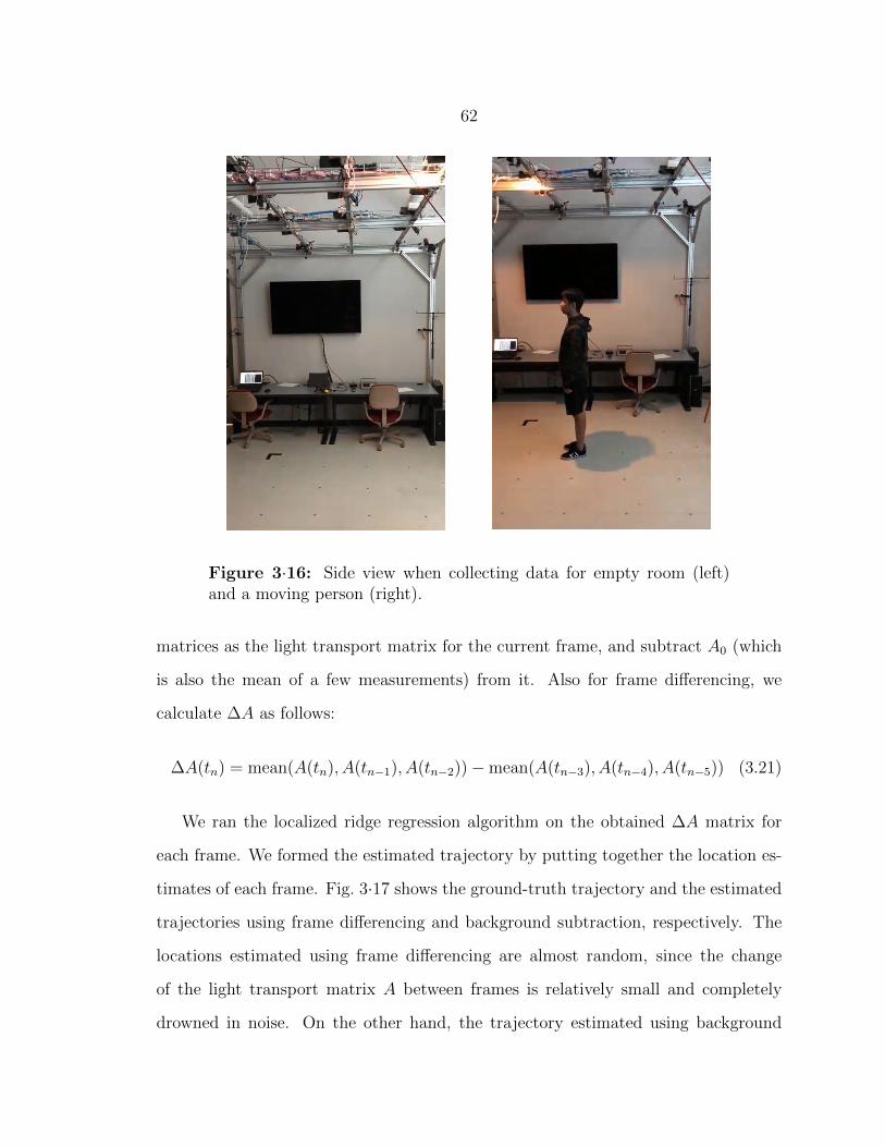
62
Figure 3·16: Side view when collecting data for empty room (left)and a moving person (right).
matrices as the light transport matrix for the current frame, and subtract A0 (which
is also the mean of a few measurements) from it. Also for frame differencing, we
calculate ∆A as follows:
∆A(tn) = mean(A(tn), A(tn−1), A(tn−2))−mean(A(tn−3), A(tn−4), A(tn−5)) (3.21)
We ran the localized ridge regression algorithm on the obtained ∆A matrix for
each frame. We formed the estimated trajectory by putting together the location es-
timates of each frame. Fig. 3·17 shows the ground-truth trajectory and the estimated
trajectories using frame differencing and background subtraction, respectively. The
locations estimated using frame differencing are almost random, since the change
of the light transport matrix A between frames is relatively small and completely
drowned in noise. On the other hand, the trajectory estimated using background

63
0 50 100 150 200 250x (cm)
0
50
100
150
200
y (
cm
)
Start
Finish
Ground-truth locationsGround-truth trajectoryEstimated trajectory
(a) Frame differencing
0 50 100 150 200 250x (cm)
0
50
100
150
200
y (
cm
)
Start
Finish
Ground-truth locationsGround-truth trajectoryEstimated trajectory
(b) Background subtraction
Figure 3·17: Ground-truth and estimated trajectories of a personwalking through 20 locations on the floor in the room-scale testbed.∆A matrices are obtained using frame differencing and backgroundsubtraction respectively. The person walks from the bottom-left cornerof the floor to the top-right corner.
subtraction basically follows the ground-truth trajectory, with reasonable localiza-
tion errors. The average localization error across all frames is 23.04cm. This suggests
that a background (empty room) measurement is still needed even when we localize
a moving object.
3.6.3 Multiple object localization
We assumed in Section 3.1 that the albedo change caused by appearance of an object
should mostly be concentrated in one connected blob. In the case of multiple objects,
we hold the same assumption, assuming that the albedo change should be concen-
trated in multiple blobs, one for each object. We slightly modified the localized ridge
regression algorithm for multiple objects as follows: after thresholding the initial esti-
mate ∆α∗0 and obtaining the set Q (Eq. (3.15)), we divide points in Q into connected
components, and each connected component is considered as an object unless it is too
small. The second step is the same as Eq. (3.16), and the estimated location of each

64
object is the centroid of ∆α∗ inside each connected component. We tested multiple
object localization with two human avatars in the Unity3D-simulated room described
in Section 3.5.1. Two samples of the localization of two avatars at different distances
are shown in Fig. 3·18. When two avatars are far enough from each other, the albedo
(a) Two avatars far from each other (b) Two avatars close to each other
Figure 3·18: Two samples of the localization of two human avatarsin Unity3D simulation. The algorithm will distinguish the two avatarsonly when they are far enough from each other.
change can be separated into two connected components; when they are close by, the
two connected components will merge into one.
We also varied the distance between the two avatars from 40cm to 240cm. The
localization error of each avatar with respect to the distance between them is shown
in Fig. 3·19. When the distance between the avatars is below 160cm, the albedo
changes caused by the two avatars are indistinguishable.

65
160 180 200 220 240Distance between two avatars (cm)
0
5
10
15
20
25
30
35
Localiz
ation e
rror
(cm
)
Avatar 1Avatar 2
Figure 3·19: Localization errors of two human avatars with respectto the distance between them in Unity3D simulation.
3.7 Estimation of light contribution matrix C
In Section 3.1 we introduced the light contribution matrix C, which can be calculated
from the knowledge of room geometry, light source and sensor positions, and light
intensity distribution function q(·). However, such knowledge is not always available,
as it takes a significant amount of effort to measure source/sensor locations in a
certain coordinate system, and a Lux meter to measure the q(·) function. Also,
these measurements can be inaccurate. In such cases, we seek to estimate the light
contribution matrix C by first sampling measurements of C (for all source-sensor
pairs) at a few locations on the floor, and then reconstructing the entire C matrix
from the sampled measurements. We studied the effect of sampling density on both
the reconstruction quality and the localization error.
3.7.1 Sampling of matrix C
A row of matrix C (C(i, j; :, :)) can be represented as a map of contributions of
different parts of the floor to the amount of luminous flux from source j to sensor i
(value A(i, j)). An example of C(i, j;x, y) for a certain source-sensor pair (i, j) and

66
the magnitude of its 2D discrete Fourier transform are shown in Fig. 3·20. It can be
seen from Fig. 3·20 that the map of C(i, j;x, y) is smooth and most of its energy is
concentrated at low frequencies.
0 50 100 150 200 250x (cm)
0
50
100
150
200
y (
cm
)
0
0.2
0.4
0.6
0.8
1
Light sourceLight sensor
(a) A row of light contribution matrixC for a certain (i, j) pair, plotted as a
map.
-10 -5 0 5 10Sampling frequency in x (points per meter)
-10
-5
0
5
10
Sam
plin
g fre
quency in y
(poin
ts p
er
mete
r)
0.1
0.2
0.3
0.4
0.5
0.6
0.7
0.8
0.9
1
(b) The magnitude of the 2D discreteFourier transform F (ξ) of the map
shown in Fig. 3·20 (a).
Figure 3·20: An example of a row of light contribution matrix C fora certain source-sensor pair (i, j) and the magnitude of its 2D discreteFourier transform.
However, the signal C(i, j;x, y) is not perfectly bandlimited, as the magnitudes
of the high-frequency components in the Fourier transform are not perfectly zero.
Therefore, no matter how densely we sample the signal C(i, j;x, y), there will always
be aliasing and the signal cannot be perfectly reconstructed. The sampling density
is determined by how much aliasing we can tolerate during the sampling process.
The sparser the sampling grid, the larger the aliasing as well as the reconstruction
and localization errors. We determine the tolerance of aliasing by thresholding the
magnitude of the Fourier transform (as a fraction of the magnitude of the zero-
frequency component) and ignoring all frequency components below the threshold.
After setting the tolerance threshold, we can then determine the sampling densities
along x and y axes of the floor.

67
If we sample C(i, j;x, y) with a series of impulses centered on a lattice Λ:
C(i, j; s) =∑w∈Λ
C(i, j; s) ∗ δ(s−w) (3.22)
where s and w represent two-dimensional points in the spatial domain (floor), then
the 2D Fourier transform of the sampled C(i, j; s) will be the periodic sum of the
Fourier transform of the original C(i, j; s):
FS(ξ) =∑ω∈Γ
F (ξ − ω) (3.23)
where Γ is the reciprocal lattice of Λ, and ξ and ω represent two-dimensional points
in the frequency domain. An example of a sampling of C(i, j;x, y) and the magnitude
of its 2D discrete Fourier transform are shown in Fig. 3·21.
0 50 100 150 200 250x (cm)
0
50
100
150
200
y (
cm
)
0
0.2
0.4
0.6
0.8
1
(a) A sampling of C(i, j;x, y) on alattice Λ.
-10 -5 0 5 10Sampling frequency in x (points per meter)
-10
-5
0
5
10
Sam
plin
g fre
quency in y
(poin
ts p
er
mete
r)
0.1
0.2
0.3
0.4
0.5
0.6
0.7
0.8
0.9
1
(b) The magnitude of the 2D discreteFourier transform of the sampledC(i, j;x, y) in Fig. 3·21 (a).
Figure 3·21: An example of a sampling of C(i, j;x, y) and the mag-nitude of its 2D Fourier transform.
By the Nyquist sampling theorem, we know that when the signal spectral support
(set of frequencies with non-zero magnitudes in the Fourier transform) fits into a
unit cell of the lattice Γ, the signal can be perfectly reconstructed from its samples.

68
Otherwise, there will be aliasing. Therefore, in choosing the reciprocal lattice Γ
(which determines the sampling lattice Λ), we must ensure that the horizontal and
vertical spacing of Γ are sufficiently large such that there is no overlap between the
shifted copies of Fourier transform of the original C(i, j;x, y).
Usually the high-frequency components of the Fourier transform of C(i, j;x, y) are
not perfectly zero. Therefore, we threshold the magnitude of the Fourier transform
by a value T and obtain a supporting set Ω(i, j):
Ω(i, j) =
ξ :
|F (ξ)|maxξ |F (ξ)|
≥ T
(3.24)
where T is usually a small positive value close to zero. We ignore all frequency
components outside Ω(i, j). Then, we take the union of Ω(i, j)’s for all (i, j) pairs:
Ω =⋃(i,j)
Ω(i, j). (3.25)
The set Ω determines the bandwidth (highest frequency component) of the Fourier
transform in fx and fy axes. The reciprocal lattice Γ should ensure that there is no
overlap between the shifted copies of Ω. We use two basis vectors parallel to x and y
axes to define the lattice Γ, where
VΓ =
[fSx 00 fSy
](3.26)
is the sampling matrix of Γ. Then, the minimum sampling frequencies in fx and fy
axes should satisfy:
fSx ≥ 2Bx, fSy ≥ 2By (3.27)
where Bx and By are the bandwidth of set Ω in fx and fy axes, respectively. We
take the equal sign in Eq. (3.27) and calculate the sampling matrix VΛ of lattice Λ as
69
follows:
VΛ =
[dx 00 dy
]= V −1
Γ (3.28)
where dx and dy are the maximum sampling intervals in x and y axes, respectively.
We can tell from Eq. (3.24)-(3.28) that dx and dy (and therefore Λ) are determined by
the threshold T in Eq. (3.24). The higher the threshold T , the smaller the bandwidths
Bx and By and the larger the sampling intervals dx and dy.
Once we determine the sampling intervals, the question left is how we should
sample C(i, j;x, y) values at points (x, y) ∈ Λ. Ideally we could do the following: if
we have a flat object of negligible size, we can collect two light transport matrices:
A0 for the empty room and A when the object is placed at location (x, y). Then, the
only albedo change happens at (x, y). By Eq. (3.6), we have:
∆A(i, j) = A(i, j)− A0(i, j) =
W∫0
L∫0
C(i, j;x, y)∆α(x, y) dxdy
= C(i, j;x, y) ·∆α(x, y) · S
(3.29)
where S is the area of the object. Then, C(i, j;x, y) can be calculated using the
following equation:
C(i, j;x, y) =∆A(i, j)
∆α(x, y) · S. (3.30)
We can obtain the matrix ∆A by placing two objects with the same shape and
known (but different) albedos at the same location (x, y) on the floor and taking the
difference of the light transport matrices. In this way, ∆α(x, y) is known and S can be
calculated if the objects have a regular shape. Then, using Eq. (3.30), we can obtain
samples of C(i, j;x, y) on a lattice Λ. In practice, we cannot sample C(i, j;x, y) with
an object of negligible size since ∆A(i, j) would be so small that it would have been

70
drowned in noise. Instead, we used the 32x object (Table 2.1) for sampling and the
value obtained using Eq. (3.30) to approximate the C(i, j;x, y) value at the center
of the object. The starting point of the sampling lattice Λ is (x0, y0) = (Lobj
2,Wobj
2)
where Lobj and Wobj are the length and width of the sampling object, so that the
object is at a corner of the floor and its boundaries overlap with the floor boundaries.
3.7.2 Estimating C from samples on a lattice
After obtaining samples of C(i, j;x, y) on a lattice Λ which satisfies the Nyquist
sampling theorem, we can recover the C(i, j;x, y) map for all (x, y) locations. In this
section, we present three methods to estimate C(i, j;x, y) from samples on a lattice.
Inverse Fourier transform: The most straightforward way to obtain the signal
C(i, j; x) is to take the inverse Fourier transform of its Fourier transform F (ξ). We
can first compute the Fourier transform FS(ξ) of the sampled signal C(i, j; x), and
apply a low-pass filter to FS(ξ) to obtain F (ξ) if there is no aliasing. We define a
low-pass filter using the set Ω in Eq. (3.25):
1Ω(ξ) =
1, if ξ ∈ Ω
0, otherwise
(3.31)
Then, the original signal C(i, j; x) can be obtained by taking the inverse Fourier
transform of FS(ξ) · 1Ω(ξ):
C(i, j; x) = IFT (FS(ξ) · 1Ω(ξ))
=∑s∈Λ
|Λ| · C(i, j; s) · χΩ(s− x)(3.32)
where |Λ| is the determinant of Λ and
χΩ(x) = IFT (1Ω(ξ)) (3.33)

71
Polynomial fitting: Another way to recover the C(i, j;x, y) map is to fit a 2D
polynomial of order N to the obtained samples:
C(i, j;x, y) =N∑n=0
(n∑i=0
β(n, i)xn−iyi)
= β · v(x, y)
(3.34)
where β is a vector of coefficients β(n, i) of all polynomials, and v(x, y) is a vector of
all polynomial values for some (x, y). We then use the least squares fitting to obtain
the coefficients that minimize the error:
β∗ = arg minβ‖Cij − V · β‖2
l2(3.35)
where
Cij =
C(i, j;x1, y1)...
C(i, j;xn, yn)
, V =
v′(x1, y1)...
v′(xn, yn)
(3.36)
and (x1, y1), . . . , (xn, yn) are points on the lattice Λ. When the number of points on
the lattice Λ is greater than or equal to the number of polynomial coefficients, the
problem (3.35) has a unique solution. Otherwise, we can make the solution unique
by adding a regularization term (e.g squared l2 norm of β) with a small weight.
We evaluate the quality of reconstruction using the R2 value, a metric commonly
used to evaluate how well the data fits into a regression curve. We did not choose
the mean squared error (MSE) as the metric since there is an unknown scaling factor
in the expression of C(i, j;x, y) which is determined by the maximum light source
intensity and the area of the sensors. Instead, R2 is normalized (with a maximum of
1), which makes it easier to see how much variation in the data is explained by the

72
fitted curve. The expression of R2 is as follows:
R2 =
∑i
(C(i, j;xi, yi)− C(i, j;xi, yi))2 −
∑i
(C(i, j;xi, yi)− C(i, j;xi, yi))2
∑i
(C(i, j;xi, yi)− C(i, j;xi, yi))2
(3.37)
where (xi, yi) represents all points on the discretized floor grid with spacing δ (not on
the lattice Λ) and C(i, j;xi, yi) is the mean of all C(i, j;xi, yi) values. We estimated
C(i, j;x, y) with polynomials of order from 2 to 4 and sampling lattices Λ obtained by
setting thresholds T = 0.01, 0.05, 0.1 in Eq. (3.24) in MATLAB simulation. The mean
of R2 values among all (i, j) pairs for different polynomial orders and thresholds are
shown in Table 3.1.
Table 3.1: Mean of R2 values among all (i, j) pairs for different poly-nomial orders and thresholds using polynomial fitting. C(i, j;x, y)’sare estimated from perfect samples (sampled with object of negligiblesize).
T 0.01 0.05 0.1polynomial order = 2 0.9471 0.8765 0.8434polynomial order = 3 0.9850 0.9450 0.9323polynomial order = 4 0.9984 0.9919 0.9910
Table 3.1 suggests that approximating C(i, j;x, y) using a polynomial of order 4
achieves good quality for certain thresholds T . We will use order 4 for polynomial
fitting in subsequent experiments.
Model fitting: The most principled way to estimate C(i, j;x, y) is to fit the
sampled values with its expression derived from the light reflection model (Eq. (3.4)).
Although we have no knowledge about room dimensions and light source and sensor
locations, we can estimate them if the expression of C(i, j;x, y) is known. For sim-
plicity, we assume that the light sources are omnidirectional, i.e. q(β) = 1 for all β.

73
Then, we can rewrite the expression for C(i, j;x, y) as follows:
C(i, j;x, y) =aH3
((x−Xj)2 + (y − Yj)2 +H2)3/2((x−Xi)2 + (y − Yi)2 +H2)2(3.38)
where H is the height of the room, a is some constant factor and (Xj, Yj, H) and
(Xi, Yi, H) are the coordinates of source j and sensor i, respectively. All these vari-
ables are unknown and we wish to estimate them such that the expression best fits
the sampled measurements. We did not achieve this by minimizing the MSE between
sampled measurements and values of Eq. (3.38) at sampling locations, since the con-
stant factor a has a much larger impact on the error than other unknowns. Instead,
we maximize the cosine similarity between them. Define a function g:
g(Xj, Yj, Xi, Yi, H;x, y)
=H3
((x−Xj)2 + (y − Yj)2 +H2)3/2((x−Xi)2 + (y − Yi)2 +H2)2
(3.39)
Then, the goal is to estimate Xj, Yj, Xi, Yi and H such that g(Xj, Yj, Xi, Yi, H;x, y)
and C(i, j;x, y) differ at most by a constant factor. To achieve this, we wish to
maximize the cosine similarity between them on the lattice Λ by minimizing the
following cost function:
fij = − log
(Cij · gij
‖Cij‖l2 ‖gij‖l2
)(3.40)
where
Cij =
C(i, j;x1, y1)...
C(i, j;xn, yn)
,gij =
g(Xj, Yj, Xi, Yi, H;x1, y1)...
g(Xj, Yj, Xi, Yi, H;xn, yn)
(3.41)
and (x1, y1), . . . , (xn, yn) are points on the lattice Λ. We minimize fij using a gradient
descent algorithm. The purpose of taking the logarithm of cosine similarity between
Cij and gij is to make calculation of gradients (∂fij∂Xj
,∂fij∂Yj
,∂fij∂Xi
,∂fij∂Yi
and∂fij∂H
) easier.

74
After obtaining the optimal valuesX∗j , Y∗j , X
∗i , Y
∗i , H
∗ and the optimal g∗ij, the con-
stant multiplier a in Eq. (3.38) can be calculated by minimizing the error∥∥Cij − ag∗ij
∥∥2
l2.
This will give a closed-form solution:
a∗ =Cij · g∗ijg∗ij · g∗ij
(3.42)
Then, all the unknowns in the expression of C(i, j;x, y) (Eq. (3.38)) are estimated
and we can calculate the values of C(i, j;x, y) at all locations (x, y) on the floor.
3.7.3 Experimental results
We evaluated the performance of the three methods proposed in Section 3.7.2 through
MATLAB simulation. The room dimensions and light source and sensor locations
are the same as those of our room-scale testbed described in Section 3.5.1. As
stated in Section 3.7.1, we sampled the C(i, j;x, y) values with the 32x object (Ta-
ble 2.1). We tested with sampling lattices Λ obtained by setting the threshold
T = 0.01, 0.02, 0.05, 0.1 and 0.15. The sampling intervals dx, dy and the number
of points in the lattice Λ for different values of T are shown in Table 3.2.
Table 3.2: Sampling intervals along x and y axes (dx, dy) and numberof points in the lattice Λ for different thresholds T when sampling withthe 32x object.
T dx (cm) dy (cm) Number of points in Λ0.01 6.22 8.00 41× 22 = 9020.02 14.74 18.18 18× 10 = 1800.05 40.00 40.00 7× 5 = 350.1 56.00 66.67 5× 3 = 150.15 93.33 66.67 3× 3 = 9
For each threshold T (and sampling lattice Λ accordingly), we first computed
the sampled values C(i, j;x, y) for all (i, j) pairs and all (x, y) points in Λ using the
procedure described in Section 3.5.1, and then applied the three proposed methods

75
to estimate the matrix C row by row. An example of original C(i, j;x, y) (calculated
using Eq.(3.4)) and the three estimated C(i, j;x, y)’s for a certain (i, j) pair is shown
in Fig. 3·22. It is clear from Fig. 3·22 that the C(i, j;x, y) map estimated with model
fitting is the closest to the original C(i, j;x, y).
0 50 100 150 200 250x (cm)
0
50
100
150
200
y (
cm
)
0
0.2
0.4
0.6
0.8
1
(a) Original C(i, j;x, y) map and thesampling lattice Λ.
0 50 100 150 200 250x (cm)
0
50
100
150
200
y (
cm
)
0
0.2
0.4
0.6
0.8
1
(b) C(i, j;x, y) estimated using inverseFourier transform.
0 50 100 150 200 250x (cm)
0
50
100
150
200
y (
cm
)
0
0.2
0.4
0.6
0.8
1
(c) C(i, j;x, y) estimated usingpolynomial fitting of order 4.
0 50 100 150 200 250x (cm)
0
50
100
150
200
y (
cm
)
0
0.2
0.4
0.6
0.8
1
(d) C(i, j;x, y) estimated using modelfitting.
Figure 3·22: An example of original C(i, j;x, y) and estimated
C(i, j;x, y)’s using three proposed methods in Section 3.7.2. The sam-pling lattice Λ is obtained by setting T = 0.15, which results in 9sampling points.
Using the estimated C matrices via the three methods, we ran the localized ridge
regression algorithm to localize a flat rectangular object on the floor. Fig. 3·23 shows
the average localization errors with respect to threshold T for estimated C matrices

76
using the three methods, when localizing the 1x and 64x objects. The performance
of the inverse Fourier transform method fluctuates due to boundary effects (sampling
lattice Λ is finite, and for some choices of T there will be large margins that are
not sampled); the polynomial fitting method performs well when T ≤ 0.05, but its
error increases significantly when T gets larger; the model fitting method performs
consistently well for T values up to 0.15, when there are as few as 9 sampling points.
This suggests that model fitting is the most robust method to sparse sampling, which
is expected since we have knowledge of the model; the expression of the model is
supposed to fit better to the sampled values than a polynomial or inverse Fourier
transform.
0.01 0.02 0.05 0.1 0.15Threshold T
0
2
4
6
8
10
12
14
16
18
20
Avera
ge localiz
ation e
rror
(cm
) Inverse Fourier transformPolynomial fittingModel fitting
(a) Errors when localizing the 1xobject (Table 2.1).
0.01 0.02 0.05 0.1 0.15Threshold T
0
2
4
6
8
10
12
14
16
18
20
Avera
ge localiz
ation e
rror
(cm
) Inverse Fourier transformPolynomial fittingModel fitting
(b) Errors when localizing the 64xobject (Table 2.1).
Figure 3·23: Average localization errors with respect to the thresholdT for original C and estimated C matrices across 63 ground-truth lo-cations in MATLAB simulation. Dashed lines indicate errors when usingoriginal C matrix calculated via Eq.(3.4) for localization.
We then tried to localize human avatars in Unity3D simulation using estimated C
matrices. We used the same simulated room and human avatars as described in Sec-
tion 3.5.1, and also collected light transport matrices in Unity3D simulation with the

77
32x object when sampling C(i, j;x.y) values. The average localization errors across
all human avatars using original C and estimated C matrices for different thresholds
T are shown in Fig. 3·24. Although the estimated C matrices using all three methods
perform only slightly worse than the original C matrix, the model fitting method no
longer outperforms the other two methods. Furniture and wall reflections can intro-
duce errors in the sampling of C(i, j;x.y) values; human avatars have complicated
shapes and textures unlike flat objects; the objective function (Eq. (3.40)) for esti-
mating the model parameters is non-convex, which makes model fitting sensitive to
noise. All these factors affect the estimation quality of model fitting, causing it to
perform not as well as in MATLAB simulations.
0.01 0.02 0.05 0.1 0.15Threshold T
0
5
10
15
20
25
30
Ave
rag
e lo
ca
liza
tio
n e
rro
r (c
m)
Inverse Fourier transformPolynomial fittingModel fitting
Figure 3·24: Average localization errors with respect to the thresholdT for original C and estimated C matrices across all human avatars inUnity3D simulation. Dashed line indicates error when using original Cmatrix for localization.
3.7.4 Conclusions
In this section, we proposed three ways to estimate the light contribution matrix C
from a few samples when the parameters needed to compute C are not known. In

78
idealized MATLAB simulations, the C matrix estimated via model fitting achieves good
accuracy with as few as 9 sampling points, which outperforms the other two methods
since the sampled values of C are supposed to follow the expressions given by the
model. In Unity3D simulations, the model fitting method with 9 sampling points
performs only slightly worse than using the original C matrix, although it does not
outperform the other two methods due to higher sensitivity to noise.
3.8 Localization with apertures on light sensors
In previous sections, we used single-pixel light sensors which output one intensity
reading - the total luminous flux that is received by the sensor. However, when taking
the sum of luminous fluxes from all incoming directions, the directional information
of reflected light is lost. This information is very useful for localization since one can
infer the object location from the directions of reflected light that is changed due to
object appearance. In this section, we propose one way to separate received light
according to incoming directions for more precise localization.
We achieve this by adding an aperture grid to each sensor. An aperture grid
consists of a set of apertures which can be turned on or off to allow or block incom-
ing light from certain directions and a cover which determines the sensor’s field of
view, as shown in Fig. 3·25. In practice, an aperture grid can be implemented using
programmable liquid crystal devices. By modulating the aperture grid, we can ob-
tain luminous flux intensities from multiple directions rather than a single aggregated
intensity.
We modified our localized ridge regression algorithm as follows for localization
with aperture grids on sensors. Instead of source-sensor pairs (i, j), we consider pairs
between a light source j and the k-th aperture of a sensor i, denoted as ((i, k), j).
Under this setting, the light transport matrix and light contribution matrix become

79
Figure 3·25: Illustration of an aperture grid on a sensor.
A((i, k), j) and C((i, k), j;x, y), respectively, both with Ns × Na rows where Na is
the number of apertures on each aperture grid. The expression of C((i, k), j;x, y)
becomes as follows:
C((i, k), j;x, y) =
ImaxSq(βj) cos βj cos2 θi
16π2Dj2(H2 + li
2),if light ray from (x, y) to
sensor i goes throughaperture k
0 , otherwise
(3.43)
where βj, Dj, θi and li are functions of x and y and are shown in Fig. 2·1, q(·) is the
light intensity distribution function of the sources and H is the room height. The new
light transport matrix A((i, k), j) can be obtained by modulating both light sources
and aperture grids following a similar procedure to the one in Section 3.2. After
obtaining the new light transport matrix A (and therefore ∆A) and contribution
matrix C, we use the same localized ridge regression algorithm as in Section 3.3.2 for
localization. The optimal solution of ∆α is expected to be more accurate since we
now have Na times the number of equations in problem (3.7).
We experimented in MATLAB simulation with the same room size and source/sensor

80
placements as our room-scale testbed (Section 3.5.1). We set the field of view of
a sensor such that each sensor looks at an area of size 1.02m×0.78m on the floor
(Fig. 3·26). This ensures that any point on the floor is in the field of view of at least
Figure 3·26: The area on the floor corresponding to a sensor and itsapertures’ field of view.
one sensor. Within a sensor’s field of view, we divided the aperture grid into 1 × 1,
2 × 2, 3 × 3 and 4 × 4 apertures, and for each grid configuration, we localized the
1x, 4x, 16x and 64x objects (Table 2.1), each placed at 63 ground-truth locations.
The average localization errors for different grid configurations and object sizes are
shown in Fig. 3·27. We noticed that the average localization error decreases when we
increase the number of apertures in each grid. This is expected since we have more
information about incoming light. However, sensors with 1 × 1 and 2 × 2 aperture
grids perform worse than sensors without aperture grids, since the aperture grids limit
the sensors’ field of view and any location on the floor is covered by fewer sensors.
Therefore, we increased the sensors’ field of view by enlarging the size of the
aperture grids. The increased field of view ensures that every sensor can see the
entire floor (as in previous experiments when there is no aperture grid on sensors).
This ensures that any location on the floor is seen by all sensors. When enlarging the
aperture grid size, we keep the grid spacing unchanged and only extend apertures on

81
1x 4x 16x 64xObject size
0
0.5
1
1.5
2
2.5
Ave
rag
e lo
ca
liza
tio
n e
rro
r (c
m)
No aperture grid1x1 aperture grid2x2 aperture grid3x3 aperture grid4x4 aperture grid
Figure 3·27: Average localization errors for different aperture gridconfigurations and object sizes. Dashed line indicates errors for sensorswithout aperture grids.
the boundaries of the grid, as illustrated in Fig. 3·28.
We repeated the MATLAB simulation experiments for enlarged aperture grids. The
average localization errors for different grid configurations and object sizes are shown
in Fig. 3·29. Compared with the performance of original grid size, the enlarged grid
size performs much better.
We also compared the estimated albedo change maps for sensors without aperture
grids and sensors with enlarged aperture grids (Fig. 3·30). The albedo change estimate
is more accurate (closer to the true shape of the object) when 3 × 3 aperture grids
are applied to sensors.

82
Figure 3·28: Illustration of an enlarged aperture grid on a sensor.
1x 4x 16x 64xObject size
0
0.5
1
1.5
2
2.5
Avera
ge localiz
ation e
rror
(cm
)
1x1 aperture grid1x1 aperture grid (enlarged)2x2 aperture grid2x2 aperture grid (enlarged)3x3 aperture grid3x3 aperture grid (enlarged)4x4 aperture grid4x4 aperture grid (enlarged)
Figure 3·29: Average localization errors for different aperture gridconfigurations and object sizes. Dashed line indicates original aperturegrids and solid lines indicate enlarged grids.

83
(a) No aperture grid, 4x object (b) Enlarged 3× 3 aperture grid, 4xobject
(c) No aperture grid, 64x object (d) Enlarged 3× 3 aperture grid, 64xobject
Figure 3·30: Estimated albedo change maps for sensors without aper-ture grids and sensors with enlarged 3×3 aperture grids when localizingthe 4x and 64x objects. Red: positive ∆α, green: negative ∆α.

84
3.9 Summary
In this chapter, we proposed localization algorithms based on the active illumina-
tion methodology. Using the relationship between modulated light source intensities
and single-pixel sensor responses, described as the light transport matrix A, the ac-
tive illumination methodology is theoretically more robust to ambient illumination
changes than passive illumination. We proposed two variants of localization algo-
rithms, namely LASSO and localized ridge regression, where the latter has a better
performance overall. In simulated (MATLAB and Unity3D) experiments, we demon-
strated that the localized ridge regression algorithm is as accurate as passive illumi-
nation when localizing flat objects, but it is significantly more robust to sensor noise
and ambient illumination changes than passive illumination. In the real testbed, the
localized ridge regression algorithm performs much better than passive illumination
due to higher robustness to noise. We also demonstrated via Unity3D simulations and
our room-scale testbed that the localized ridge regression algorithm is still accurate
when localizing human occupants, although the model assumes that objects should
be flat.
Moving forward, we extended our framework to 3D, moving and multiple objects.
We proposed a more principled shadow-based algorithm for 3D object localization,
which is found to have similar performance to the localized ridge regression algorithm.
For moving objects, the localized ridge regression algorithm works well when the
change of light transport matrix ∆A is obtained by subtracting background (A0)
from current measurements (A). Multiple objects can be localized simultaneously by
performing connected component detection on the estimated albedo change map, but
objects can become indistinguishable when they get close to each other.
We also studied the problem of estimating the light contribution matrix C from
samples when room dimensions and source/sensor locations are not available. We de-

85
termined the sampling lattice via 2D Fourier spectrum analysis, and proposed three
ways to estimate matrix C - inverse Fourier transform, polynomial fitting and model
fitting. The model fitting approach is the most principled since it fits the expression of
C into the obtained samples, and it does perform the best in MATLAB simulations, es-
pecially when there are very few sampling points. However, in the Unity3D-simulated
room with human avatars, it does not outperform the other two approaches as it is
more sensitive to sampling noise.
Finally, we proposed a new sensor design using aperture grids. By separating
incoming luminous flux according to directions, we can obtain directional information
about light that has changed due to object appearance. As a result, the localization
accuracy is improved and the estimated albedo changes are more accurate.

86
Chapter 4
Data-driven approaches to indoor
localization via active scene illumination
In Chapter 3 we introduced our model-based localized ridge regression algorithm via
active illumination, which can accurately localize a flat object or a human occupant.
However, the model-based algorithm has strict modeling assumptions on the prop-
erties of the floor, walls or object, which are not always satisfied in practice. Such
deviations from the modeling assumptions can decrease the algorithm’s performance.
Also, the algorithm requires either knowledge of room dimensions, source/sensor lo-
cations and characteristics, or a set of sampled values of the light contribution matrix
C, both of which cannot be obtained easily.
Therefore, in this chapter, we explored data-driven approaches to localization via
active illumination, which require only a training dataset and a machine learning
model. Modeling assumptions or knowledge of geometries are no longer required - all
they require is a good training set that covers a wide variety of scenarios.
We use the change of light transport matrix between empty and occupied room
states ∆A = A − A0 as the feature, and the object (or occupant) location (x, y)
as the label. The estimations of location along x and y axes are considered as two
regression problems. We will consider both classical data-driven approaches and
neural networks.

87
4.1 Classical data-driven approaches
For classical data-driven approaches, we consider support vector regression (SVR)
and K-nearest neighboor (KNN) regression. In these two approaches, we pre-process
the input feature as follows - we first normalize the matrix ∆A by dividing all its
entries by the magnitude of the entry with the largest absolute value:
∆A′ =∆A
maxi,j
(|∆Aij|)(4.1)
such that all entries of ∆A′ lie in the interval [−1, 1]; then, the flattened ∆A′ matrix
is used as the input feature vector to the models.
4.1.1 Support vector regression (SVR)
The support vector regression (SVR) is a variant of the support vector machine (SVM)
for binary classification. In SVR, we wish to find a function that maps a feature vector
x to a real value:
f(x) = K(β,x) + b (4.2)
where K(·, ·) = 〈φ(·), φ(·)〉 is a positive-definite and symmetric kernel, and b is a
constant. Similar to classification SVM, we want to minimize the norm of β:
min1
2‖β‖2
l2(4.3)
subject to the following constraints:
|yi −K(β,x)− b| ≤ ε, ∀i (4.4)
where yi is the label of the i-th training sample and ε is the tolerance of regression
errors. Since there may not exist a vector β that satisfies all the constraints (4.4), we

88
form the following optimization problem by introducing slack variables ξi and ξ∗i :
min1
2‖β‖2
l2+B
N∑i=1
(ξi + ξ∗i )
subject to yi −K(β,x)− b ≤ ε+ ξi, ∀i
− yi +K(β,x) + b ≤ ε+ ξ∗i , ∀i
ξi ≥ 0, ∀i
ξ∗i ≥ 0, ∀i
(4.5)
where N is the number of training samples and B is called the box constraint, which
controls the trade-off between bias and variance. By solving the dual problem of
problem (4.5), we obtain the optimal function to predict new values given feature
vectors:
f ∗(x) =N∑i=1
(αi − α∗i )K(xi,x) + b (4.6)
where ai and a∗i satisfy the following constraints:
N∑i=1
(αi − α∗i ) = 0
0 ≤ αi ≤ B, ∀i
0 ≤ α∗i ≤ B, ∀i
(4.7)
The training samples xi with regression error less than ε satisfy αi = 0 and α∗i = 0.
If either αi = 0 or α∗i = 0 is not satisfied, the training sample is called a support
vector, and only support vectors determine the predicted value of the regressor.
In our experiments, we trained two support vector regressors to estimate object
location (x, y) along both axes. We used the radial basis function (RBF) as the
kernel, and found the optimal parameters ε and B on a two-dimensional grid via a
5-fold cross-validation.
89
4.1.2 K-nearest neighbor (KNN) regression
In KNN regression, the predicted value of a feature vector is determined by the labels
of its K nearest neighbors in the training set with the smallest distances to the feature
vector. The choice of a distance metric in the feature-vector space may vary, and we
chose Euclidean distance as the metric:
d(x,xi) = ‖x− xi‖l2 (4.8)
The reason behind this choice is as follows. By Eq. (3.6), we have
∆A(i, j) = C(i, j;x, y) ·∆α · S (4.9)
where (x, y) is the object location, when the object area S W×L. Since C(i, j;x, y)
is continuous and rather smooth (Fig. 3·20 (a)) for all (i, j) pairs, when the object
is moved by a small distance, all the ∆A(i, j) values will change by a small amount;
when the object movement is large, it is unlikely that the changes of ∆A(i, j) values
for all (i, j) pairs will remain small, since sources and sensors are placed at different
locations across the entire ceiling. Also, the effect of scaling by ∆α · S is eliminated
since we have normalized ∆A (Eq. (4.1)). Therefore, a small distance in the feature-
vector (∆A′) space corresponds to a small distance in the (x, y) space. One can also
use l1, l3, . . . , l∞ distances instead of l2 distance.
For a test sample, we first compute its distance to all data samples in the training
set, and then sort the distances and find the K smallest ones. The predicted location
of the test sample is given as the weighted centroid of the ground-truth locations of
the K nearest neighbors:
x =K∑i=1
wixi, y =K∑i=1
wiyi (4.10)

90
where (xi, yi) is the ground-truth location of the i-th nearest neighbor, and the weights
wi are proportional to the reciprocal of the Euclidean distances:
wi =
1
d(x,xi)K∑i=1
1
d(x,xi)
. (4.11)
The parameter K is optimized through grid search and 5-fold cross-validation.
4.2 Convolutional neural network (CNN) approach
Besides classical data-driven approaches, we also consider CNN-based approaches.
CNNs are popular for their good performance on image data, where they make use
of spatial correlation between adjacent pixels in an image by applying convolutional
kernels. Also, the number of parameters is greatly reduced compared with a fully-
connected neural network, which makes training much faster and reduces overfitting.
Although our input feature (∆A′) is not a typical image, we can reshape it to
make use of spatial correlation between sensors. We note that sensors closer to the
occupant should have larger reading changes between empty and occupied room states
than those further away. To leverage this spatial relationship, we reshape the Ns×Nf
matrix ∆A′ into a 3D tensor of Nf channels. Each channel consists of entries from
one column of ∆A′ corresponding to the contribution of light from a light source to all
sensors, and is reshaped into a 2D matrix to match the spatial ordering of the actual
sensor grid on the ceiling. This will allow the network to extract the occupant’s
location from the channel images. Fig. 4·1 shows an example of the original ∆A′
matrix and the reshaped 3D tensor.
We have 12 light sources and 12 sensors placed on a 3× 4 grid in our room-scale
testbed. Therefore, the reshaped input has 12 channels, and each channel contains
a 3× 4 “image” of light transport matrix changes. For this “image” size, the choice

91
(a) Original ∆A′ matrix.In our room-scale
testbed, we have Ns = 12and Nf = 12.
(b) Reshaped 3D tensor with Nf = 12channels. Each channel is reshaped into a3× 4 matrix corresponding to the actual
sensor grid.
Figure 4·1: Example of an original ∆A′ matrix and its reshaped 3Dtensor form. Red boxes correspond to the same entries. Occupant islocated at the lower right corner of the floor.
of convolutional kernel and stride sizes is very limited. Therefore, to allow sub-pixel
kernel and stride sizes, we upsample the channel “images” using bilinear interpolation
with several upsampling factors.
We proposed a CNN with 4 layers: 2 convolutional layers, 1 hidden layer and
1 output layer. The first two convolutional layers have 32 and 64 output channels
and use 2D convolutional kernels. The second convolutional layer is flattened and
then fully connected with the hidden layer. The hidden layer is fully connected with
the output layer which gives the estimated occupant location (x, y). The kernel and
stride sizes of the two convolutional layers and the dimension of the hidden layer are
chosen according to the upsampling factor of the input (which determines the input
size), that are listed in Table 4.1. The loss function is the mean squared localization
error (squared Euclidean distance between estimated and ground truth locations). To
avoid the problem of vanishing gradients, the outputs of the two convolutional layers
and the hidden layer are activated by a LeakyReLU function with α = 0.1. Figure

92
Table 4.1: Parameters of our proposed CNN for different upsamplingfactors.
Upsampling factor 1 3 5 10Input channel size 3×4 7×10 11×16 21×31Conv1 kernel size 2×2 4×4 4×4 6×6Conv1 stride size (1,1) (1,1) (2,2) (2,2)Conv2 kernel size 2×2 2×2 3×3 4×4Conv2 stride size (1,1) (1,1) (1,1) (2,2)
Dimension of hidden layer 170 300 500 750
4·2 illustrates the overall architecture of the CNN.
Figure 4·2: Architecture of our proposed CNN. See Table 4.1 fordetails.
4.3 Experimental results
To validate and compare the performance of the classical data-driven approaches and
our proposed CNN, we performed experiments in both Unity3D simulations with hu-
man avatars and our room-scale testbed with occupants. The experimental settings
and data collection process are described in Section 3.5.1 and Section 3.5.2 respec-
tively.

93
4.3.1 Simulation experiments
As stated in Section 3.5.2, we collected 63 × 8 = 504 data samples using 8 human
avatars in Unity3D simulation. These samples are used as the test set. We collected
another dataset for training using the same 8 avatars, each placed at 1,530 ground-
truth locations on a 45× 34 grid with 5cm spacing. There is no overlap between the
training and test set grids.
We considered two different scenarios when training the classical data-driven mod-
els and our proposed CNN: private and public. In a private scenario, like a home, the
system can only be used by a small set of people, and most of the time, the system
will see users which it has encountered before. Therefore, we can train a model with
data from all human avatars and test on the same avatars. In a public scenario, like
a store, the model cannot be trained on all users since there can always be new users
that have not been seen by the system. In this case, we have to train with data from
all but one human avatar and test on the excluded avatar.
In the private scenario, out of 1,530×8 training samples we use only 50×8 samples
(50 random samples for each avatar) for training. This is to simulate the real-world
scenario when we have few training data. All the data-driven models are trained
using the same set of samples. Then, we test each model on each avatar’s 63 test
samples (with 25cm spacing) which are separate from the larger training set of 1530×8
samples. In the public scenario, we perform a leave-one-person-out cross-validation.
We train a model on 7 avatars (50 samples per avatar) and test it on the eighth avatar,
and repeat this process 8 times so that each of the avatars is left out for testing. The
performance of a model is evaluated in terms of average localization error.
We tested several choices of the upsampling factor for the input tensor of our CNN:
1 (no upsampling), 3, 5 and 10. As the input size is scaled, we scale the network to
roughly match the input size by changing the network parameters (Table 4.1). The

94
Table 4.2: Average localization errors of our proposed CNN for dif-ferent upsampling factors in private and public scenarios in Unity3Dsimulation.
Upsampling factor 1 3 5 10Average localization error - private (cm) 6.43 6.25 5.69 6.47Average localization error - public (cm) 7.89 7.96 8.04 8.61
network parameters and average localization errors for different upsampling factors
are shown in Table 4.2. The network with an upsampling factor of 5 performs best
in the private scenario, while performing only slightly worse than the best case in the
public scenario.
We compared the performance of SVR, KNN regression, our proposed CNN (with
an upsampling factor of 5) and our model-based localized ridge regression algorithm
(Section 3.3.2). Figure 4·3 shows the average localization errors for each human avatar
for the four methods. The CNN approach outperforms the other three methods for all
human avatars in both scenarios. It reduces the average localization error across all
avatars by 47.69% and 46.99% in private and public scenarios, respectively, compared
to the best-performing method among SVR, KNN and model-based.

95
1 2 3 4 5 6 7 8Human avatar index
0
5
10
15
20
25A
ve
rag
e lo
ca
liza
tio
n e
rro
r (c
m)
SVRKNN regressionModel-basedProposed CNN
(a) Private scenario
1 2 3 4 5 6 7 8Human avatar index
0
5
10
15
20
25
30
35
40
Ave
rag
e lo
ca
liza
tio
n e
rro
r (c
m)
SVRKNN regressionModel-basedProposed CNN
(b) Public scenario
Figure 4·3: Average localization errors for each human avatar forSVR, KNN regression, CNN and model-based (localized ridge regres-sion) algorithms in Unity3D simulation. The model-based algorithmhas the same errors in private and public scenarios since it does notneed training.
4.3.2 Testbed experiments
We performed testbed experiments using the same dataset as we used in previous
experiments (Section 3.5.2). We collected data for 8 human occupants, where each of
them walked through 63 ground-truth locations on a 9 × 7 grid with 25cm spacing.
We also considered both private and public scenarios in the testbed experiments.
In the private scenario, we randomly selected 50 samples from each person to form
the training set (totaling 400 samples), and used the remaining 13 samples of each
person as the test set (totaling 104 samples). In the public scenario, we performed
a leave-one-person-out cross-validation by training the models on 7 persons (using
63 × 7 = 441 samples) and testing on the eighth person (63 samples). The process
was repeated 8 times so that each person is left out for testing.

96
We also compared the performance of the same 4 algorithms in private and public
scenarios. For the CNN, we chose the network corresponding to the upsampling factor
of 5. Figure 4·4 shows the average localization error for each person in both scenarios.
Compared with the best-performing method (among SVR, KNN and model-based)
in each scenario, our CNN reduces the average localization error across all individuals
by 36.54% in the private scenario and by 11.46% in the public scenario.
1 2 3 4 5 6 7 8Person index
0
10
20
30
40
50
60
70
Ave
rag
e lo
ca
liza
tio
n e
rro
r (c
m)
SVRKNN regressionModel-basedProposed CNN
(a) Private scenario
1 2 3 4 5 6 7 8Person index
0
20
40
60
80
100
120
Ave
rag
e lo
ca
liza
tio
n e
rro
r (c
m)
SVRKNN regressionModel-basedProposed CNN
(b) Public scenario
Figure 4·4: Average localization errors for each person for SVR,KNN regression, CNN and model-based (localized ridge regression)algorithms in the room-scale testbed.
4.4 Transfer learning
A popular way to improve the performance of deep neural networks is to use transfer
learning. Transfer learning refers to the techniques of solving a new problem using
knowledge learned from solving a different but related problem. It is found to be
helpful when there is high correlation between the two problems, and especially when
the training set for the new problem is small. In Section 4.3, we trained our local-

97
ization CNN with around 400 samples in both private and public scenarios, which is
a very small training set, and therefore we seek to improve the performance of our
CNN using transfer learning.
There are two stages in transfer learning: offline training and fine-tuning. In
offline training, a neural network is trained from scratch with a large training set
from one domain; and in the fine-tuning stage, another network is initialized using
the weights of the pre-trained network, and then trained with a smaller training set
from another domain.
In our experiments, we first pre-trained our localization CNN (with upsampling
factor of 5) with the training samples collected in Unity3D simulation (Section 4.3.1).
All the 1,530 samples from each of the 8 avatars are used for training, totaling 12,240
samples. Then, we used the samples collected in our testbed for fine-tuning, where
we also consider private and public scenarios. During the fine-tuning stage, the pa-
rameters of the two convolutional layers are frozen, so that they become a feature
extractor. Only the parameters for the hidden output layers are updated. The aver-
age localization errors for our CNN with and without transfer learning in private and
public scenarios are shown in Fig. 4·5. In both scenarios, transfer learning did not
significantly improve the performance of the CNN, and for some avatars it performs
even slightly worse. The reason can be one of the following: either the datasets from
two domains (Unity3D and testbed) are not similar enough, or the CNN trained with
only testbed data is already close to optimal.
To figure out the reason why transfer learning does not improve performance, we
conducted another set of experiments, where both training and fine-tuning sets are
from Unity3D simulation. We collected the training set with a mannequin (human
avatar without texture) of three different sizes: small, medium and large, which are
scaled such that mannequin heights are equal to the minimum, average and maximum

98
1 2 3 4 5 6 7 8Person index
0
5
10
15
20
25
Ave
rag
e lo
ca
liza
tio
n e
rro
r (c
m)
CNN without transfer learningCNN with transfer learning
(a) Private scenario
1 2 3 4 5 6 7 8Person index
0
10
20
30
40
50
60
70
Ave
rag
e lo
ca
liza
tio
n e
rro
r (c
m)
CNN without transfer learningCNN with transfer learning
(b) Public scenario
Figure 4·5: Average localization errors for our CNN with and with-out transfer learning in private and public scenarios in the room-scaletestbed. The training-and-test splits of data in both scenarios are thesame as those in Section 4.3.2.
heights of the 8 human avatars. Fig. 4·6 shows the mannequin used in our experi-
ments. Mannequin of each size is placed at the same 1,530 ground-truth locations as
those in Section 4.3.1. We trained the CNN with 1, 530 × 3 = 4, 590 samples from
the mannequin, and fine-tuned it with the same samples used to train the CNN for
private and public scenarios in Section 4.3.1.
Fig. 4·7 shows a comparison of average localization errors with and without trans-
fer learning in both scenarios. Even when the training and fine-tuning datasets are
extremely similar, the fine-tuned CNN only reduces average localization error across
all human avatars by 1.34% and 3.71% in private and public scenarios, respectively,
compared with the CNN trained from scratch. This suggests that the CNN trained
from scratch with the fine-tuning set (400 samples in private scenario, 350 in public
scenario) is already close to its optimal, which is expected since the size and number
of parameters of our CNN is small compared with the majority of CNNs.

99
Figure 4·6: The mannequin used in Unity3D simulation to collecttraining data.
1 2 3 4 5 6 7 8Human avatar index
0
2
4
6
8
10
12
14
Ave
rag
e lo
ca
liza
tio
n e
rro
r (c
m)
CNN without transfer learningCNN with transfer learning
(a) Private scenario
1 2 3 4 5 6 7 8Human avatar index
0
2
4
6
8
10
12
14
Ave
rag
e lo
ca
liza
tio
n e
rro
r (c
m)
CNN without transfer learningCNN with transfer learning
(b) Public scenario
Figure 4·7: Average localization errors for our CNN with and withouttransfer learning in private and public scenarios in Unity3D simulation.In transfer learning, the CNN is pre-trained with data samples from themannequin.

100
4.5 Robustness to sensor failures
In Chapter 3, we evaluated our algorithm’s robustness against noise and ambient
illumination changes. Besides these non-idealities, failures of light sources or sensors
can also happen and affect the algorithm’s performance. Light source failures can
be easily detected by human eyes, as the failed light sources will stop illuminating;
however, failures of light sensors are much harder to detect since they are not visible.
In this section, we will test the robustness of our model-based localized ridge regression
algorithm and our CNN against sensor failures.
We assume that a failed sensor will constantly output zero readings. To simulate
sensor failure using already collected datasets, we first computed change of light
transport matrix ∆A, and then set ∆A(i, j) = 0 for all sources j and all failed sensor
indexes i. The processed ∆A matrix is then fed into the model-based algorithm or
the CNN as input.
We experimented with data from both Unity3D simulations and the room-scale
testbed. We used the same datasets used in Section 3.5.2, each having 63× 8 = 504
samples collected from 8 avatars/persons. We varied the number of failed sensors from
1 to 11. For each specified number of failed sensors Nfail, we randomly selected Nfail
sensors out of Ns sensors, and set the corresponding ∆A entries to zero. This process
was repeated 3 times and the localization errors from 3 repetitions were averaged. For
the model-based algorithm, there are two options: after setting ∆A(i, j) = 0 for failed
sensors, we can either zero the rows of light contribution matrix C corresponding to
failed sensors, as if the failed sensors do not exist; or we can just keep matrix C as
it is. Also when testing the CNN, we divided the dataset into 3 folds, and for each
Nfail and each repetition, we performed a 3-fold cross-validation and averaged the
localization errors of all folds. Note that the data folds used for training do not take
failed sensors into account; only failed sensor readings in the test fold are set to zero.

101
0 1 2 3 4 5 6 7 8 9 10 11Number of failed sensors
0
20
40
60
80
100
120
140
Ave
rag
e lo
ca
liza
tio
n e
rro
r (c
m)
Model-based algorithm (keep matrix C)Model-based algorithm (zero rows of C)CNN
(a) Unity3D simulation
0 1 2 3 4 5 6 7 8 9 10 11Number of failed sensors
0
20
40
60
80
100
120
140
Ave
rag
e lo
ca
liza
tio
n e
rro
r (c
m)
Model-based algorithm (keep matrix C)Model-based algorithm (zero rows of C)CNN
(b) Room-scale testbed
Figure 4·8: Average localization errors with respect to the number offailed sensors for the model-based algorithm and the CNN in Unity3Dsimulation and the testbed. Both options for the model-based algorithmare tested.
Fig. 4·8 shows the average localization error with respect to the number of failed
sensors for model-based algorithm and CNN in Unity3D simulations and testbed.
The localization errors for the model-based algorithm (if we choose to keep matrix
C) and the CNN increase at similar rates as the number of failed sensors increases,
and the model-based algorithm always has a higher error than the CNN. However,
if we choose to zero the rows of C corresponding to failed sensors, the localization
error for the model-based algorithm decreases significantly compared to the other
two cases, and remains almost constant when Nfail ≤ 6 in both Unity3D simulations
and the testbed. This is to be expected since the model equation (Eq. (3.6)) is not
violated when we completely remove a sensor and the corresponding rows of matrix
C; it is violated when we have wrong sensor readings.

102
4.6 Summary
In this chapter, we explored several data-driven approaches to localization via ac-
tive scene illumination, including SVR, KNN regression and a proposed CNN model.
Compared with model-based algorithms, data-driven approaches do not require any
modeling assumptions or knowledge of room geometry and source/sensor character-
istics. We compared the three data-driven approaches as well as the model-based lo-
calized ridge regression algorithm, and our proposed CNN outperforms all the other
methods in private and public scenarios in both Unity3D simulations and the real
testbed, with only around 400 training samples.
We also sought to improve the performance of our CNN using transfer learning.
However, when we trained the CNN with a large Unity3D dataset and fine-tuned it
with testbed data, there is no improvement compared with the CNN trained form
scratch with only testbed data. The improvement is minimal even when we trained
with data from a Unity3D mannequin and tested with Unity3D human avatars. This
suggests that the CNN trained from scratch is already close to optimal since it is a
small network.
Finally, we evaluated the robustness of the model-based algorithm and the CNN
to sensor failures. The two approaches have similar error increases as the number of
failed sensors increases, while the model-based algorithm has slightly higher errors.
However, if we could detect the failed sensors and remove the corresponding entries
of the light transport matrix A and rows of light contribution matrix C, the model-
based algorithm will become much more robust to sensor failures and perform well
even when half of the sensors have failed.

103
Chapter 5
Conclusions
5.1 Summary of the dissertation
This dissertation proposed an active illumination methodology which aims to accom-
plish three goals for an indoor occupant localization system: accuracy, robustness
and privacy preservation. In our system, an array of single-pixel light sensors is used
to preserve visual privacy of room occupants, while modulated LED light sources are
used to improve the system’s robustness to noise and illumination changes. To assure
accurate localization, we explored and proposed both model-based and data-driven
algorithms.
The model-based algorithm is derived under the assumption that both the floor
and the object are Lambertian and flat. Using Lambert’s Cosine Law, the model
relates the change of light received by sensors to the change of floor albedo due to
the presence of an object. Our proposed localized ridge regression algorithm esti-
mates floor albedo change and object location based on the change of light transport
matrix and parameters of the room and light sources/sensors. We demonstrated via
simulation and testbed experiments that the proposed algorithm is more robust to
noise and illumination changes than the model-based passive illumination algorithm,
and more robust to sensor failures than data-driven approaches. The proposed algo-
rithm can also accurately localize 3D (e.g., human occupants), moving and multiple
objects under certain circumstances. Furthermore, we proposed ways to estimate
the light contribution matrix C when information about room geometry and light

104
sources/sensors is not available, and a sensor design with aperture grids which im-
proves localization accuracy.
On the other hand, we also explored data-driven approaches that do not require
modeling assumptions or room, source or sensor parameters. We proposed a convolu-
tional neural network (CNN) for localization, where we reshaped the light transport
matrix as input such that the CNN can take advantage of spatial correlations between
sensors. As a result, the proposed CNN outperforms support vector regression (SVR),
K-nearest neighbor (KNN) regression and the model-based algorithm in localization
of human occupants. Also, experiments with transfer learning demonstrated that a
small training set (≈400 samples) is enough for the CNN to achieve good performance.
However, there is a trade-off between localization accuracy and ease of implemen-
tation. The CNN-based approach performs much better in realistic scenarios, since
the model learns the real-world non-idealities (e.g., 3D shapes of human occupants,
furniture, indirect light) from the training data. But a good training dataset can be
expensive to collect in a real testbed, which is a large amount of effort when deploy-
ing the system into a new room. By contrast, the model-based approach requires
strict modeling assumptions about the room, light, floor and object, which are not
always satisfied in reality, but if we know the light source locations (e.g., via the
CAD blueprint of the room) and have a device that can measure the sensor locations
(e.g., a calibrated camera where sensors can be detected in the captured image), then
it is much easier to deploy the system into a new room than using the CNN-based
approach. Therefore, we need choose the method that best fits the usage scenarios
and requirements for accuracy.

105
5.2 Future directions
This dissertation is a first step towards privacy-preserving indoor localization via
active scene illumination, which mainly focuses on algorithm development and exper-
imental validation. In addition to these, the following directions could be of potential
interest to future researchers.
In our testbed, we used 12 light sources and 12 sensors and achieved good accuracy.
However, experimental results in Fig. 4·8 suggest that we could remove a few sensors
and still maintain good performance. Therefore, one interesting direction could be
finding the minimum number of sources and sensors needed to achieve a certain level
of accuracy using theoretical analysis. One could try to derive theoretical bounds for
localization error or reconstruction error of ∆α, which is related to the number and
locations of sources and sensors.
Another direction could be exploring the type of light sources or sensors used.
Currently, our LEDs and single-pixel sensors both work in the visible light spectrum.
These can be replaced with infrared light sources and sensors to make the flicker
invisible to human eyes. One could also consider infrared light sources that generate
structured light and infrared cameras that capture the pattern. In this way, we could
reconstruct the scene in 3D and localize multiple objects more accurately. Besides
localization, other indoor activity analysis tasks necessary for future smart room
applications, including action recognition and pose estimation, could be explored.

106
Appendix A
Closed-form Solution to Ridge Regression
Problem
The minimization problem (3.14) can be re-written as:
∆α∗0 =arg min∆α
[∥∥∆A− δ2C∆α∥∥2
l2+ σδ2 ‖∆α‖2
l2
]=arg min
∆α
[∆AT∆A− 2δ2∆ATC∆α+ δ4∆αTCTC∆α+ σδ2∆αT∆α
]=arg min
∆α
[∆αT(δ2CTC + σI)∆α− 2∆ATC∆α
].
(A.1)
Let g(∆α) = ∆αT(δ2CTC + σI)∆α − 2∆ATC∆α. The function g(∆α) is a
quadratic function of ∆α and the matrix δ2CTC +σI is positive definite (we assume
δ, σ > 0). The optimal solution is obtained by setting its gradient to zero:
∇g(∆α) = 2(δ2CTC + σI)∆α− 2CT∆A = 0
⇒ ∆α∗0 = (δ2CTC + σI)−1CT∆A.(A.2)
For problem (3.16), we define vector ∆α′ as a sub-vector of ∆α containing only
∆α(x, y) values where (x, y) ∈ Q, and C ′ as a sub-matrix of C containing only the
columns corresponding to floor grid points inside Q. Similarly, the optimal ∆α′∗ can
also be calculated in closed form:
∆α′∗ = (δ2C ′TC ′ + σI)−1C ′T∆A. (A.3)
The optimal ∆α∗ is then obtained by padding zeros into ∆α′∗ that correspond to
points (x, y) 6∈ Q.

References
Bitouk, D., Kumar, N., Dhillon, S., Belhumeur, P., and Nayar, S. K. (2008). Faceswapping: automatically replacing faces in photographs. In ACM Transactions onGraphics (TOG), volume 27, page 39. ACM.
Boyle, M., Edwards, C., and Greenberg, S. (2000). The effects of filtered video onawareness and privacy. In Proceedings of the 2000 ACM conference on Computersupported cooperative work, pages 1–10. ACM.
Brkic, K., Sikiric, I., Hrkac, T., and Kalafatic, Z. (2017). I know that person:Generative full body and face de-identification of people in images. In 2017 IEEEConference on Computer Vision and Pattern Recognition Workshop (CVPRW),pages 1319–1328.
Brumitt, B., Meyers, B., Krumm, J., Kern, A., and Shafer, S. (2000). Easyliving:Technologies for intelligent environments. In International Symposium on Hand-held and Ubiquitous Computing, pages 12–29. Springer.
Chen, J., Wu, J., Richter, K., Konrad, J., and Ishwar, P. (2016). Estimating headpose orientation using extremely low resolution images. In 2016 IEEE SouthwestSymposium on Image Analysis and Interpretation (SSIAI), pages 65–68. IEEE.
Dai, J., Wu, J., Saghafi, B., Konrad, J., and Ishwar, P. (2015). Towards privacy-preserving activity recognition using extremely low temporal and spatial resolutioncameras. In Proceedings of the IEEE Conference on Computer Vision and PatternRecognition Workshops, pages 68–76.
De Lausnay, S., De Strycker, L., Goemaere, J.-P., Stevens, N., and Nauwelaers, B.(2015). A visible light positioning system using frequency division multiple accesswith square waves. In 2015 9th International Conference on Signal Processing andCommunication Systems (ICSPCS), pages 1–7. IEEE.
Dufaux, F. (2011). Video scrambling for privacy protection in video surveillance:recent results and validation framework. In Mobile Multimedia/Image Processing,Security, and Applications 2011, volume 8063, page 806302. International Societyfor Optics and Photonics.
Dufaux, F. and Ebrahimi, T. (2006). Scrambling for video surveillance with privacy.In 2006 IEEE Conference on Computer Vision and Pattern Recognition Workshops(CVPRW), pages 160–160. IEEE.
107

108
Dufaux, F. and Ebrahimi, T. (2008). Scrambling for privacy protection in videosurveillance systems. IEEE Transactions on Circuits and Systems for Video Tech-nology, 18(8):1168–1174.
Erdelyi, A., Barat, T., Valet, P., Winkler, T., and Rinner, B. (2014). Adaptivecartooning for privacy protection in camera networks. In 2014 11th IEEE Interna-tional Conference on Advanced Video and Signal Based Surveillance (AVSS), pages44–49. IEEE.
Erdelyi, A., Winkler, T., and Rinner, B. (2013). Serious fun: Cartooning for pri-vacy protection. In MediaEval 2013 Multimedia Benchmark Workshop. CEURWorkshop Proceedings, volume 1043.
Frazier, L. M. (1996). Surveillance through walls and other opaque materials. In Pro-ceedings of the 1996 IEEE National Radar Conference, 1996, pages 27–31. IEEE.
Frome, A., Cheung, G., Abdulkader, A., Zennaro, M., Wu, B., Bissacco, A., Adam,H., Neven, H., and Vincent, L. (2009). Large-scale privacy protection in googlestreet view. In 2009 IEEE 12th International Conference on Computer Vision(ICCV), pages 2373–2380.
Gilad-Bachrach, R., Dowlin, N., Laine, K., Lauter, K., Naehrig, M., and Wernsing,J. (2016). Cryptonets: Applying neural networks to encrypted data with highthroughput and accuracy. In International Conference on Machine Learning, pages201–210.
Gross, R., Airoldi, E., Malin, B., and Sweeney, L. (2005). Integrating utility into facede-identification. In International Workshop on Privacy Enhancing Technologies,pages 227–242. Springer.
Gross, R., Sweeney, L., De la Torre, F., and Baker, S. (2006). Model-based facede-identification. In 2006 IEEE Conference on Computer Vision and PatternRecognition Workshop (CVPRW), page 161. IEEE.
Hassan, E. T., Hasan, R., Shaffer, P., Crandall, D., and Kapadia, A. (2017). Car-tooning for enhanced privacy in lifelogging and streaming videos. In Proceedingsof the IEEE Conference on Computer Vision and Pattern Recognition Workshops(CVPRW), pages 29–38.
Hauschildt, D. and Kirchhof, N. (2010). Advances in thermal infrared localization:Challenges and solutions. In 2010 International Conference on Indoor Positioningand Indoor Navigation, pages 1–8. IEEE.
Hightower, J., Want, R., and Borriello, G. (2000). Spoton: An indoor 3d locationsensing technology based on rf signal strength. UW CSE 00-02-02, University ofWashington, Department of Computer Science and Engineering, Seattle, WA, 1.

109
Huang, Q., Ge, Z., and Lu, C. (2016). Occupancy estimation in smart buildingsusing audio-processing techniques. arXiv preprint arXiv:1602.08507.
Jia, L. and Radke, R. J. (2014). Using time-of-flight measurements for privacy-preserving tracking in a smart room. IEEE Transactions on Industrial Informatics,10(1):689–696.
Kim, H.-S., Kim, D.-R., Yang, S.-H., Son, Y.-H., and Han, S.-K. (2013). An in-door visible light communication positioning system using a rf carrier allocationtechnique. Journal of Lightwave Technology, 31(1):134–144.
Kohoutek, T. K., Mautz, R., and Donaubauer, A. (2010). Real-time indoor position-ing using range imaging sensors. In Real-Time Image and Video Processing 2010,volume 7724, page 77240K. International Society for Optics and Photonics.
Kosba, A. E., Abdelkader, A., and Youssef, M. (2009). Analysis of a device-freepassive tracking system in typical wireless environments. In 2009 3rd InternationalConference on New Technologies, Mobility and Security (NTMS), pages 1–5. IEEE.
Krumm, J. (2016). Ubiquitous computing fundamentals. CRC Press.
Kuroiwa, K., Fujiyoshi, M., and Kiya, H. (2007). Codestream domain scramblingof moving objects based on dct sign-only correlation for motion jpeg movies. In2007 IEEE International Conference on Image Processing (ICIP), volume 5, pagesV–157. IEEE.
Li, T., Liu, Q., and Zhou, X. (2016). Practical human sensing in the light. InProceedings of the 14th Annual International Conference on Mobile Systems, Ap-plications, and Services, pages 71–84. ACM.
Ma, L., Zhang, Z., and Tan, X. (2006). A novel through-wall imaging method usingultra wideband pulse system. In 2006 International Conference on IntelligentInformation Hiding and Multimedia Signal Processing (IIH-MSP), pages 147–150.IEEE.
Macq, B. M. and Quisquater, J.-J. (1995). Cryptology for digital tv broadcasting.Proceedings of the IEEE, 83(6):944–957.
Mandal, A., Lopes, C. V., Givargis, T., Haghighat, A., Jurdak, R., and Baldi, P.(2005). Beep: 3d indoor positioning using audible sound. In 2005 Second IEEEConsumer Communications and Networking Conference (CCNC), pages 348–353.IEEE.
Martınez-Ponte, I., Desurmont, X., Meessen, J., and Delaigle, J.-F. (2005). Robusthuman face hiding ensuring privacy. In Proceedings of the International Workshopon Image Analysis for Multimedia Interactive Services, volume 4.

110
Misra, P. and Enge, P. (1999). Special issue on global positioning system. Proceed-ings of the IEEE, 87(1):3–15.
Moussa, M. and Youssef, M. (2009). Smart devices for smart environments: Device-free passive detection in real environments. In 2009 IEEE International Conferenceon Pervasive Computing and Communications (PerCom), pages 1–6. IEEE.
Munoz-Salinas, R., Medina-Carnicer, R., Madrid-Cuevas, F. J., and Carmona-Poyato,A. (2009). Multi-camera people tracking using evidential filters. InternationalJournal of Approximate Reasoning, 50(5):732–749.
Nadeem, U., Hassan, N., Pasha, M., and Yuen, C. (2015). Indoor positioning systemdesigns using visible led lights: performance comparison of tdm and fdm protocols.Electronics Letters, 51(1):72–74.
Neustaedter, C. and Greenberg, S. (2003). The design of a context-aware homemedia space for balancing privacy and awareness. In International Conference onUbiquitous Computing, pages 297–314. Springer.
Neustaedter, C., Greenberg, S., and Boyle, M. (2006). Blur filtration fails to preserveprivacy for home-based video conferencing. ACM Transactions on Computer-Human Interaction (TOCHI), 13(1):1–36.
Newton, E. M., Sweeney, L., and Malin, B. (2005). Preserving privacy by de-identifying face images. IEEE transactions on Knowledge and Data Engineering,17(2):232–243.
Ni, L. M., Liu, Y., Lau, Y. C., and Patil, A. P. (2004). Landmarc: indoor locationsensing using active rfid. Wireless networks, 10(6):701–710.
Petrushin, V. A., Wei, G., and Gershman, A. V. (2006). Multiple-camera peo-ple localization in an indoor environment. Knowledge and Information Systems,10(2):229–241.
Pittaluga, F. and Koppal, S. J. (2015). Privacy preserving optics for miniature visionsensors. In Proceedings of the IEEE Conference on Computer Vision and PatternRecognition, pages 314–324.
Priyantha, N. B., Chakraborty, A., and Balakrishnan, H. (2000). The cricketlocation-support system. In Proceedings of the 6th annual international confer-ence on Mobile computing and networking, pages 32–43. ACM.
Raval, N., Machanavajjhala, A., and Cox, L. P. (2017). Protecting visual secretsusing adversarial nets. In 2017 IEEE Conference on Computer Vision and PatternRecognition Workshops (CVPRW), pages 1329–1332. IEEE.

111
Reijniers, J. and Peremans, H. (2007). Biomimetic sonar system performing spectrum-based localization. IEEE Transactions on Robotics, 23(6):1151–1159.
Roeper, D., Chen, J., Konrad, J., and Ishwar, P. (2016). Privacy-preserving, in-door occupant localization using a network of single-pixel sensors. In 2016 13thIEEE International Conference on Advanced Video and Signal Based Surveillance(AVSS), pages 214–220. IEEE.
Ryoo, M. S., Rothrock, B., Fleming, C., and Yang, H. J. (2017). Privacy-preservinghuman activity recognition from extreme low resolution. In 31st AAAI Conferenceon Artificial Intelligence (AAAI), pages 4255–4262.
Sadeghi, A.-R., Schneider, T., and Wehrenberg, I. (2009). Efficient privacy-preservingface recognition. In International Conference on Information Security and Cryp-tology, pages 229–244. Springer.
Senior, A., Pankanti, S., Hampapur, A., Brown, L., Tian, Y.-L., Ekin, A., Connell, J.,Shu, C. F., and Lu, M. (2005). Enabling video privacy through computer vision.IEEE Security & Privacy, 3(3):50–57.
Steendam, H. (2018). A 3-d positioning algorithm for aoa-based vlp with an aperture-based receiver. IEEE Journal on Selected Areas in Communications, 36(1):23–33.
Vongkulbhisal, J., Chantaramolee, B., Zhao, Y., and Mohammed, W. S. (2012). Afingerprinting-based indoor localization system using intensity modulation of lightemitting diodes. Microwave and Optical Technology Letters, 54(5):1218–1227.
Wan, E. A. and Paul, A. S. (2010). A tag-free solution to unobtrusive indoor trackingusing wall-mounted ultrasonic transducers. In 2010 International Conference onIndoor Positioning and Indoor Navigation (IPIN), pages 1–10. IEEE.
Wang, Q., Zhang, X., and Boyer, K. L. (2014). Occupancy distribution estimationfor smart light delivery with perturbation-modulated light sensing. Journal ofsolid state lighting, 1(1):17.
Wang, W., Vong, C.-M., Yang, Y., and Wong, P.-K. (2017). Encrypted imageclassification based on multilayer extreme learning machine. MultidimensionalSystems and Signal Processing, 28(3):851–865.
Wang, X. and Wang, S. (2007). Collaborative signal processing for target track-ing in distributed wireless sensor networks. Journal of Parallel and DistributedComputing, 67(5):501–515.
Wang, Z., Chang, S., Yang, Y., Liu, D., and Huang, T. S. (2016). Studying very lowresolution recognition using deep networks. In Proceedings of the IEEE Conferenceon Computer Vision and Pattern Recognition, pages 4792–4800.

112
Want, R., Hopper, A., Falcao, V., and Gibbons, J. (1992). The active badge locationsystem. ACM Transactions on Information Systems (TOIS), 10(1):91–102.
Wilson, J. and Patwari, N. (2009). Through-wall tracking using variance-based radiotomography networks. arXiv preprint arXiv:0909.5417.
Yang, S.-H., Kim, H.-S., Son, Y.-H., and Han, S.-K. (2014). Three-dimensionalvisible light indoor localization using aoa and rss with multiple optical receivers.Journal of Lightwave Technology, 32(14):2480–2485.
Ye, G. (2010). Image scrambling encryption algorithm of pixel bit based on chaosmap. Pattern Recognition Letters, 31(5):347–354.
Youssef, M., Mah, M., and Agrawala, A. (2007). Challenges: device-free passivelocalization for wireless environments. In Proceedings of the 13th annual ACM in-ternational conference on Mobile computing and networking, pages 222–229. ACM.
Zajdel, W. and Krose, B. J. (2005). A sequential bayesian algorithm for surveillancewith nonoverlapping cameras. International Journal of Pattern Recognition andArtificial Intelligence, 19(08):977–996.
Zeng, W. and Lei, S. (2003). Efficient frequency domain selective scrambling ofdigital video. IEEE Transactions on Multimedia, 5(1):118–129.
Zhang, C., Rui, Y., and He, L.-w. (2006). Light weight background blurring forvideo conferencing applications. In 2006 IEEE International Conference on ImageProcessing (ICIP), pages 481–484.
Zhang, W., Chowdhury, M. S., and Kavehrad, M. (2014). Asynchronous indoorpositioning system based on visible light communications. Optical Engineering,53(4):045105.
Ziad, M. T. I., Alanwar, A., Alzantot, M., and Srivastava, M. (2016). Cryptoimg:Privacy preserving processing over encrypted images. In 2016 IEEE Conferenceon Communications and Network Security (CNS), pages 570–575. IEEE.

CURRICULUM VITAE
Jinyuan Zhao
[email protected] of Electrical and Computer Engineering, Boston University
8 Saint Mary’s St, Boston, MA 02215
EDUCATION
Boston University, Boston, MA, USA Sep 2015 - PresentPh.D. Candidate in Electrical and Computer Engineering
Tsinghua University, Beijing, China Sep 2011 - Jul 2015B.Eng in Electronic Information Sciences
PROFESSIONAL EXPERIENCE
Graduate Research Assistant Feb 2016 - PresentVisual Information Processing (VIP) Lab, Department of Electrical and Computer
Engineering, Boston University
Graduate Teaching Assistant Feb 2017 - Dec 2017Department of Electrical and Computer Engineering, Boston University
Software Engineer Intern May 2019 - Aug 2019Avigilon Corp., Somerville, MA
HONORS AND AWARDS
Student Poster Competition Winner Jan 201714th US Dept. of Energy Solid State Lighting R&D Workshop
Oral Presenter Oct 2016New England Computer Vision Workshop
Scholarship on Improvement in Studies Oct 2012Tsinghua University

114
PUBLICATIONS
• J. Zhao, N. Frumkin, P. Ishwar, and J. Konrad , CNN-based Indoor OccupantLocalization via Active Scene Illumination, Accepted by 2019 25th IEEE Inter-national Conference on Image Processing (ICIP), Taipei, Taiwan, 22-25 Sep.,2019.
• J. Zhao, N. Frumkin, J. Konrad, and P. Ishwar, Privacy-preserving IndoorLocalization via Active Scene Illumination, in Proc. IEEE Conference on Com-puter Vision and Pattern Recognition Workshops (CVPRW), Salt Lake City,UT, 18-22 Jun., 2018, pp. 1580–1589.
• J. Zhao, P. Ishwar, and J. Konrad, Privacy-Preserving Indoor Localization viaLight Transport Analysis, in Proc. IEEE International Conference on Acous-tics, Speech, and Signal Processing (ICASSP), New Orleans, LA, 5-9 Mar., 2017,pp. 3331–3335.