bose–einstein condensation in dilute gases second
TRANSCRIPT

BOSE–EINSTEIN CONDENSATIONIN DILUTE GASES
Second Edition
Since an atomic Bose–Einstein condensate, predicted by Einstein in 1925, wasfirst produced in the laboratory in 1995, the study of ultracold Bose and Fermigases has become one of the most active areas in contemporary physics. Inthis book the authors explain phenomena in ultracold gases from basic prin-ciples, without assuming a detailed knowledge of atomic and condensed mat-ter physics. This new edition has been revised and updated, and includes newchapters on optical lattices, low dimensions, and strongly interacting Fermisystems.
This book provides a unified introduction to the physics of ultracold atomicBose and Fermi gases at advanced undergraduate and graduate levels. The bookwill also be of interest to anyone with a general background in physics, fromundergraduates to researchers in the field. Chapters cover the statistical phys-ics of trapped gases, atomic properties, cooling and trapping atoms, interatomicinteractions, structure of trapped condensates, collective modes, rotating condens-ates, superfluidity, mixtures and spinor condensates, interference and correlations,optical lattice low-dimensional systems, Fermi gases and the crossover from theBCS superfluid state to a Bose–Einstein condensate of diatomic molecules. Prob-lems are included at the end of each chapter.
Christopher Pethick graduated with a D.Phil. in 1965 from the Universityof Oxford, and he had a research fellowship there until 1970. During the years1966–69 he was a postdoctoral fellow at the University of Illinois at Urbana–Champaign, where he joined the faculty in 1970, becoming Professor of Physicsin 1973. Following periods spent at the Landau Institute for Theoretical Physics,Moscow and at Nordita (Nordic Institute for Theoretical Physics), Copenhagen,as a visiting scientist, he accepted a permanent position at Nordita in 1975, anddivided his time for many years between Nordita and the University of Illinois.Apart from the subject of the present book, Professor Pethick’s main researchinterests are condensed matter physics (quantum liquids, especially 3He, 4He andsuperconductors) and astrophysics (particularly the properties of dense matter andthe interiors of neutron stars). He is also the co-author of Landau Fermi-LiquidTheory: Concepts and Applications (1991).

Henrik Smith obtained his mag. scient. degree in 1966 from the University ofCopenhagen and spent the next few years as a postdoctoral fellow at CornellUniversity and as a visiting scientist at the Institute for Theoretical Physics,Helsinki. In 1972 he joined the faculty of the University of Copenhagen wherehe became dr. phil. in 1977 and Professor of Physics in 1978. He has alsoworked as a guest scientist at the Bell Laboratories, New Jersey. Professor Smith’sresearch field is condensed matter physics and low-temperature physics, includingquantum liquids and the properties of superfluid 3He transport properties ofnormal and superconducting metals and two-dimensional electron systems. Hisother books include Transport Phenomena (1989) and Introduction to QuantumMechanics (1991).
The two authors have worked together on problems in low-temperature physics,in particular on the superfluid phases of liquid 3He superconductors and dilutequantum gases. This book derives from graduate-level lectures given by theauthors at the University of Copenhagen.

BOSE–EINSTEIN CONDENSATIONIN DILUTE GASES
Second Edition
C. J. PETHICKNordita
H. SMITHUniversity of Copenhagen

cambridge univers ity press
Cambridge, New York, Melbourne, Madrid, Cape Town, Singapore, São Paulo
Cambridge University PressThe Edinburgh Building, Cambridge CB2 8RU, UK
Published in the United States of America by Cambridge University Press, New York
www.cambridge.orgInformation on this title: www.cambridge.org/9780521846516
© C. Pethick and H. Smith 2008
This publication is in copyright. Subject to statutory exceptionand to the provisions of relevant collective licensing agreements,
no reproduction of any part may take place withoutthe written permission of Cambridge University Press.
First published 2001Second Edition 2008
Printed in the United Kingdom at the University Press, Cambridge
A catalogue record for this publication is available from the British Library
ISBN 978-0-521-84651-6 hardback
Cambridge University Press has no responsibility for the persistence oraccuracy of URLs for external or third-party internet websites referred to
in this publication, and does not guarantee that any content on suchwebsites is, or will remain, accurate or appropriate.

Contents
Preface page xiii
1 Introduction 11.1 Bose–Einstein condensation in atomic clouds 41.2 Superfluid 4He 71.3 Other condensates 91.4 Overview 10
Problems 15References 15
2 The non-interacting Bose gas 172.1 The Bose distribution 17
2.1.1 Density of states 192.2 Transition temperature and condensate fraction 21
2.2.1 Condensate fraction 242.3 Density profile and velocity distribution 25
2.3.1 The semi-classical distribution 282.4 Thermodynamic quantities 33
2.4.1 Condensed phase 332.4.2 Normal phase 352.4.3 Specific heat close to Tc 36
2.5 Effect of finite particle number 38Problems 39References 40
3 Atomic properties 413.1 Atomic structure 413.2 The Zeeman effect 453.3 Response to an electric field 50
v

vi Contents
3.4 Energy scales 56Problems 58References 59
4 Trapping and cooling of atoms 604.1 Magnetic traps 61
4.1.1 The quadrupole trap 624.1.2 The TOP trap 644.1.3 Magnetic bottles and the Ioffe–Pritchard trap 664.1.4 Microtraps 69
4.2 Influence of laser light on an atom 714.2.1 Forces on an atom in a laser field 754.2.2 Optical traps 77
4.3 Laser cooling: the Doppler process 784.4 The magneto-optical trap 824.5 Sisyphus cooling 844.6 Evaporative cooling 964.7 Spin-polarized hydrogen 103
Problems 106References 107
5 Interactions between atoms 1095.1 Interatomic potentials and the van der Waals interaction 1105.2 Basic scattering theory 114
5.2.1 Effective interactions and the scattering length 1195.3 Scattering length for a model potential 1255.4 Scattering between different internal states 130
5.4.1 Inelastic processes 1355.4.2 Elastic scattering and Feshbach resonances 143
5.5 Determination of scattering lengths 1515.5.1 Scattering lengths for alkali atoms and hydrogen 154Problems 156References 156
6 Theory of the condensed state 1596.1 The Gross–Pitaevskii equation 1596.2 The ground state for trapped bosons 162
6.2.1 A variational calculation 1656.2.2 The Thomas–Fermi approximation 168
6.3 Surface structure of clouds 1716.4 Healing of the condensate wave function 175

Contents vii
6.5 Condensates with dipolar interactions 176Problems 179References 180
7 Dynamics of the condensate 1827.1 General formulation 182
7.1.1 The hydrodynamic equations 1847.2 Elementary excitations 1887.3 Collective modes in traps 196
7.3.1 Traps with spherical symmetry 1977.3.2 Anisotropic traps 2007.3.3 Collective coordinates and the variational method 204
7.4 Surface modes 2117.5 Free expansion of the condensate 2137.6 Solitons 215
7.6.1 Dark solitons 2167.6.2 Bright solitons 222Problems 223References 224
8 Microscopic theory of the Bose gas 2258.1 The uniform Bose gas 226
8.1.1 The Bogoliubov transformation 2298.1.2 Elementary excitations 2308.1.3 Depletion of the condensate 2318.1.4 Ground-state energy 2338.1.5 States with definite particle number 234
8.2 Excitations in a trapped gas 2368.3 Non-zero temperature 241
8.3.1 The Hartree–Fock approximation 2428.3.2 The Popov approximation 2488.3.3 Excitations in non-uniform gases 2508.3.4 The semi-classical approximation 251References 253
9 Rotating condensates 2559.1 Potential flow and quantized circulation 2559.2 Structure of a single vortex 257
9.2.1 A vortex in a uniform medium 2579.2.2 Vortices with multiple quanta of circulation 2619.2.3 A vortex in a trapped cloud 262

viii Contents
9.2.4 An off-axis vortex 2659.3 Equilibrium of rotating condensates 265
9.3.1 Traps with an axis of symmetry 2669.3.2 Rotating traps 2679.3.3 Vortex arrays 270
9.4 Experiments on vortices 2739.5 Rapidly rotating condensates 2759.6 Collective modes in a vortex lattice 280
Problems 286References 288
10 Superfluidity 29010.1 The Landau criterion 29110.2 The two-component picture 294
10.2.1 Momentum carried by excitations 29410.2.2 Normal fluid density 295
10.3 Dynamical processes 29610.4 First and second sound 30010.5 Interactions between excitations 307
10.5.1 Landau damping 308Problems 314References 315
11 Trapped clouds at non-zero temperature 31611.1 Equilibrium properties 317
11.1.1 Energy scales 31711.1.2 Transition temperature 31911.1.3 Thermodynamic properties 321
11.2 Collective modes 32511.2.1 Hydrodynamic modes above Tc 328
11.3 Collisional relaxation above Tc 33411.3.1 Relaxation of temperature anisotropies 33911.3.2 Damping of oscillations 342Problems 345References 346
12 Mixtures and spinor condensates 34812.1 Mixtures 349
12.1.1 Equilibrium properties 35012.1.2 Collective modes 354
12.2 Spinor condensates 356

Contents ix
12.2.1 Mean-field description 35812.2.2 Beyond the mean-field approximation 360Problems 363References 364
13 Interference and correlations 36513.1 Tunnelling between two wells 365
13.1.1 Quantum fluctuations 37113.1.2 Squeezed states 373
13.2 Interference of two condensates 37413.2.1 Phase-locked sources 37513.2.2 Clouds with definite particle number 381
13.3 Density correlations in Bose gases 38413.3.1 Collisional shifts of spectral lines 386
13.4 Coherent matter wave optics 39013.5 Criteria for Bose–Einstein condensation 394
13.5.1 The density matrix 39413.5.2 Fragmented condensates 397Problems 399References 399
14 Optical lattices 40114.1 Generation of optical lattices 402
14.1.1 One-dimensional lattices 40314.1.2 Higher-dimensional lattices 40614.1.3 Energy scales 407
14.2 Energy bands 40914.2.1 Band structure for a single particle 40914.2.2 Band structure for interacting particles 41114.2.3 Tight-binding model 416
14.3 Stability 41814.3.1 Hydrodynamic analysis 421
14.4 Intrinsic non-linear effects 42314.4.1 Loops 42314.4.2 Spatial period doubling 427
14.5 From superfluid to insulator 43114.5.1 Mean-field approximation 43314.5.2 Effect of trapping potential 43914.5.3 Experimental detection of coherence 439Problems 441References 442

x Contents
15 Lower dimensions 44415.1 Non-interacting gases 44515.2 Phase fluctuations 447
15.2.1 Vortices and the Berezinskii–Kosterlitz–Thouless transi-tion 451
15.3 Microscopic theory of phase fluctuations 45315.3.1 Uniform systems 45515.3.2 Anisotropic traps 456
15.4 The one-dimensional Bose gas 46015.4.1 The strong-coupling limit 46115.4.2 Arbitrary coupling 46615.4.3 Correlation functions 474Problems 479References 480
16 Fermions 48116.1 Equilibrium properties 48316.2 Effects of interactions 48616.3 Superfluidity 489
16.3.1 Transition temperature 49116.3.2 Induced interactions 49616.3.3 The condensed phase 498
16.4 Pairing with unequal populations 50616.5 Boson–fermion mixtures 508
16.5.1 Induced interactions in mixtures 509Problems 511References 513
17 From atoms to molecules 51417.1 Bose–Einstein condensation of molecules 51617.2 Diatomic molecules 518
17.2.1 Binding energy and the atom–atom scattering length 51817.2.2 A simple two-channel model 52017.2.3 Atom–atom scattering 526
17.3 Crossover: From BCS to BEC 52717.3.1 Wide and narrow Feshbach resonances 52817.3.2 The BCS wave function 53017.3.3 Crossover at zero temperature 53117.3.4 Condensate fraction and pair wave function 535
17.4 Crossover at non-zero temperature 54017.4.1 Thermal molecules 540

Contents xi
17.4.2 Pair fluctuations and thermal molecules 54317.4.3 Density of atoms 54817.4.4 Transition temperature 549
17.5 A universal limit 55017.6 Experiments in the crossover region 553
17.6.1 Collective modes 55317.6.2 Vortices 556Problems 559References 560
Appendix. Fundamental constants and conversion factors 562Index 564


Preface
The experimental discovery of Bose–Einstein condensation in trappedatomic clouds opened up the exploration of quantum phenomena in a qual-itatively new regime. Our aim in the present work is to provide an intro-duction to this rapidly developing field.
The study of Bose–Einstein condensation in dilute gases draws on manydifferent subfields of physics. Atomic physics provides the basic methodsfor creating and manipulating these systems, and the physical data requiredto characterize them. Because interactions between atoms play a key rolein the behaviour of ultracold atomic clouds, concepts and methods fromcondensed matter physics are used extensively. Investigations of spatial andtemporal correlations of particles provide links to quantum optics, whererelated studies have been made for photons. Trapped atomic clouds havesome similarities to atomic nuclei, and insights from nuclear physics havebeen helpful in understanding their properties.
In presenting this diverse range of topics we have attempted to explainphysical phenomena in terms of basic principles. In order to make the pre-sentation self-contained, while keeping the length of the book within reason-able bounds, we have been forced to select some subjects and omit others.For similar reasons and because there now exist review articles with exten-sive bibliographies, the lists of references following each chapter are far fromexhaustive.
This book originated in a set of lecture notes written for a graduate-level one-semester course on Bose–Einstein condensation at the Universityof Copenhagen. The first edition was completed in 2001. For this second edi-tion we have updated the manuscript and added three new chapters on opti-cal lattices, lower dimensions and molecules. We employ SI units throughoutthe text. As for mathematical notation we generally use ∼ to indicate ‘is oforder’, while � means ‘is asymptotically equal to’ as in (1 − x)−1 � 1 + x.
xiii

xiv Preface
The symbol ≈ means ‘is approximately equal to’. Definitions are indicatedby ≡, and ∝ means ‘is proportional to’. However, the reader should beaware that strict consistency in these matters is not possible.
We have received much inspiration from contacts with our colleagues inboth experiment and theory. In particular we thank Gordon Baym, GeorgBruun, Alexander Fetter, Henning Heiselberg, Andreas Isacsson, GeorgeKavoulakis, Pietro Massignan, Ben Mottelson, Jorg Helge Muller, AlexandruNicolin, Nicolai Nygaard, Olav Syljuasen, Gentaro Watanabe and MikhailZvonarev for many stimulating and helpful discussions over the past fewyears. Wolfgang Ketterle kindly provided us with the cover illustration andFig. 13.2, and we thank Eric Cornell for allowing us to use Fig. 9.3. Weare grateful to Mikhail Zvonarev for providing us with the data for Figs.15.2–4. The illustrations in the text have been prepared by Janus Schmidtand Alexandru Nicolin, whom we thank for a pleasant collaboration. It isa pleasure to acknowledge the continuing support of Simon Capelin, SusanFrancis and Lindsay Barnes at the Cambridge University Press, and thecareful copy-editing of the manuscript by Brian Watts and Jon Billam.

1
Introduction
The experimental realization in 1995 of Bose–Einstein condensation in di-lute atomic gases marked the beginning of a very rapid development in thestudy of quantum gases. The initial experiments were performed on vapoursof rubidium [1], sodium [2], and lithium [3].1 So far, the atoms 1H, 7Li, 23Na,39K, 41K, 52Cr, 85Rb, 87Rb, 133Cs, 170Yb, 174Yb and 4He* (the helium atomin an excited state) have been demonstrated to undergo Bose–Einstein con-densation. In related developments, atomic Fermi gases have been cooled towell below the degeneracy temperature, and a superfluid state with corre-lated pairs of fermions has been observed. Also molecules consisting of pairsof fermionic atoms such as 6Li or 40K have been observed to undergo Bose–Einstein condensation. Atoms have been put into optical lattices, therebyallowing the study of many-body systems that are realizations of modelsused in condensed matter physics. Although the gases are very dilute, theatoms can be made to interact strongly, thus providing new challenges forthe description of strongly correlated many-body systems. In a period ofless than ten years the study of dilute quantum gases has changed from anesoteric topic to an integral part of contemporary physics, with strong tiesto molecular, atomic, subatomic and condensed matter physics.
The dilute quantum gases differ from ordinary gases, liquids and solidsin a number of ways, as we shall now illustrate by giving values of physi-cal quantities. The particle density at the centre of a Bose–Einstein con-densed atomic cloud is typically 1013–1015 cm−3. By contrast, the densityof molecules in air at room temperature and atmospheric pressure is about1019 cm−3. In liquids and solids the density of atoms is of order 1022 cm−3,while the density of nucleons in atomic nuclei is about 1038 cm−3.
To observe quantum phenomena in such low-density systems, the tem-
1 Numbers in square brackets are references, to be found at the end of each chapter.
1

2 Introduction
perature must be of order 10−5 K or less. This may be contrasted withthe temperatures at which quantum phenomena occur in solids and liquids.In solids, quantum effects become strong for electrons in metals below theFermi temperature, which is typically 104–105 K, and for phonons belowthe Debye temperature, which is typically of order 102 K. For the heliumliquids, the temperatures required for observing quantum phenomena are oforder 1 K. Due to the much higher particle density in atomic nuclei, thecorresponding degeneracy temperature is about 1011 K.
The path that led in 1995 to the first realization of Bose–Einstein conden-sation in dilute gases exploited the powerful methods developed since themid 1970s for cooling alkali metal atoms by using lasers. Since laser cool-ing alone did not produce sufficiently high densities and low temperaturesfor condensation, it was followed by an evaporative cooling stage, in whichthe more energetic atoms were removed from the trap, thereby cooling theremaining atoms.
Cold gas clouds have many advantages for investigations of quantum phe-nomena. In a weakly interacting Bose–Einstein condensate, essentially allatoms occupy the same quantum state, and the condensate may be describedin terms of a mean-field theory similar to the Hartree–Fock theory for atoms.This is in marked contrast to liquid 4He, for which a mean-field approachis inapplicable due to the strong correlations induced by the interactionbetween the atoms. Although the gases are dilute, interactions play an im-portant role as a consequence of the low temperatures, and they give rise tocollective phenomena related to those observed in solids, quantum liquids,and nuclei. Experimentally the systems are attractive ones to work with,since they may be manipulated by the use of lasers and magnetic fields. Inaddition, interactions between atoms may be varied either by using differentatomic species or, for species that have a Feshbach resonance, by changingthe strength of an applied magnetic or electric field. A further advantage isthat, because of the low density, ‘microscopic’ length scales are so large thatthe structure of the condensate wave function may be investigated directlyby optical means. Finally, these systems are ideal for studies of interferencephenomena and atom optics.
The theoretical prediction of Bose–Einstein condensation dates back morethan 80 years. Following the work of Bose on the statistics of photons [4],Einstein considered a gas of non-interacting, massive bosons, and concludedthat, below a certain temperature, a non-zero fraction of the total numberof particles would occupy the lowest-energy single-particle state [5]. In 1938Fritz London suggested the connection between the superfluidity of liquid4He and Bose–Einstein condensation [6]. Superfluid liquid 4He is the pro-

Introduction 3
totype Bose–Einstein condensate, and it has played a unique role in thedevelopment of physical concepts. However, the interaction between heliumatoms is strong, and this reduces the number of atoms in the zero-momentumstate even at absolute zero. Consequently it is difficult to measure directlythe occupancy of the zero-momentum state. It has been investigated ex-perimentally by neutron scattering measurements of the structure factor atlarge momentum transfers [7], and the results are consistent with a relativeoccupation of the zero-momentum state of about 0.1 at saturated vapourpressure and about 0.05 near the melting pressure [8].
The fact that interactions in liquid helium reduce dramatically the oc-cupancy of the lowest single-particle state led to the search for weakly in-teracting Bose gases with a higher condensate fraction. The difficulty withmost substances is that at low temperatures they do not remain gaseous,but form solids or, in the case of the helium isotopes, liquids, and the effectsof interaction thus become large. In other examples atoms first combineto form molecules, which subsequently solidify. As long ago as in 1959Hecht [9] argued that spin-polarized hydrogen would be a good candidatefor a weakly interacting Bose gas. The attractive interaction between twohydrogen atoms with their electronic spins aligned was then estimated tobe so weak that there would be no bound state. Thus a gas of hydrogenatoms in a magnetic field would be stable against formation of moleculesand, moreover, would not form a liquid, but remain a gas to arbitrarily lowtemperatures.
Hecht’s paper was before its time and received little attention, but hisconclusions were confirmed by Stwalley and Nosanow [10] in 1976, when im-proved information about interactions between spin-aligned hydrogen atomswas available. These authors also argued that because of interatomic inter-actions the system would be a superfluid as well as being Bose–Einsteincondensed. This latter paper stimulated the quest to realize Bose–Einsteincondensation in atomic hydrogen. Initial experimental attempts used ahigh magnetic field gradient to force hydrogen atoms against a cryogeni-cally cooled surface. In the lowest-energy spin state of the hydrogen atom,the electron spin is aligned opposite the direction of the magnetic field (H↓),since then the magnetic moment is in the same direction as the field. Spin-polarized hydrogen was first stabilized by Silvera and Walraven [11]. Interac-tions of hydrogen with the surface limited the densities achieved in the earlyexperiments, and this prompted the Massachusetts Institute of Technology(MIT) group led by Greytak and Kleppner to develop methods for trappingatoms purely magnetically. In a current-free region, it is impossible to createa local maximum in the magnitude of the magnetic field. To trap atoms by

4 Introduction
the Zeeman effect it is therefore necessary to work with a state of hydrogenin which the electronic spin is polarized parallel to the magnetic field (H↑).Among the techniques developed by this group is that of evaporative coolingof magnetically trapped gases, which has been used as the final stage in allexperiments to date to produce a gaseous Bose–Einstein condensate. Sincelaser cooling is not feasible for hydrogen, the gas is precooled cryogenically.After more than two decades of heroic experimental work, Bose–Einsteincondensation of atomic hydrogen was achieved in 1998 [12].
As a consequence of the dramatic advances made in laser cooling of alkaliatoms, such atoms became attractive candidates for Bose–Einstein conden-sation, and they were used in the first successful experiments to producea gaseous Bose–Einstein condensate. In later developments other atomshave been shown to undergo Bose–Einstein condensation: metastable 4Heatoms in the lowest-energy electronic spin-triplet state [13, 14], and ytter-bium [15,16] and chromium atoms [17] in their electronic ground states.
The properties of interacting Bose fluids are treated in many texts. Thereader will find an illuminating discussion in the volume by Nozieres andPines [18]. A collection of articles on Bose–Einstein condensation in vari-ous systems, prior to its discovery in atomic vapours, is given in [19], whilemore recent theoretical developments have been reviewed in [20]. The 1998Varenna lectures are a useful general reference for both experiment and the-ory on Bose–Einstein condensation in atomic gases, and contain in additionhistorical accounts of the development of the field [21]. For a tutorial reviewof some concepts basic to an understanding of Bose–Einstein condensationin dilute gases see Ref. [22]. The monograph [23] gives a comprehensiveaccount of Bose–Einstein condensation in liquid helium and dilute atomicgases.
1.1 Bose–Einstein condensation in atomic clouds
Bosons are particles with integer spin. The wave function for a systemof identical bosons is symmetric under interchange of any two particles.Unlike fermions, which have half-odd-integer spin and antisymmetric wavefunctions, bosons may occupy the same single-particle state. An order-of-magnitude estimate of the transition temperature to the Bose–Einsteincondensed state may be made from dimensional arguments. For a uniformgas of free particles, the relevant quantities are the particle mass m, thenumber of particles per unit volume n, and the Planck constant h = 2π�.The only quantity having dimensions of energy that can be formed from �,n, and m is �
2n2/3/m. By dividing this energy by the Boltzmann constant

1.1 Bose–Einstein condensation in atomic clouds 5
k we obtain an estimate of the condensation temperature Tc,
Tc = C�
2n2/3
mk. (1.1)
Here C is a numerical factor which we shall show in the next chapter tobe equal to approximately 3.3. When (1.1) is evaluated for the mass anddensity appropriate to liquid 4He at saturated vapour pressure one obtainsa transition temperature of approximately 3.13 K, which is close to thetemperature below which superfluid phenomena are observed, the so-calledlambda point2 (Tλ= 2.17 K at saturated vapour pressure).
An equivalent way of relating the transition temperature to the parti-cle density is to compare the thermal de Broglie wavelength λT with themean interparticle spacing, which is of order n−1/3. The thermal de Brogliewavelength is conventionally defined by
λT =(
2π�2
mkT
)1/2
. (1.2)
At high temperatures, it is small and the gas behaves classically. Bose–Einstein condensation in an ideal gas sets in when the temperature is so lowthat λT is comparable to n−1/3. For alkali atoms, the densities achievedrange from 1013 cm−3 in early experiments to 1014–1015 cm−3 in more re-cent ones, with transition temperatures in the range from 100 nK to a fewμK. For hydrogen, the mass is lower and the transition temperatures arecorrespondingly higher.
In experiments, gases are non-uniform, since they are contained in a trap,which typically provides a harmonic-oscillator potential. If the number ofparticles is N , the density of gas in the cloud is of order N/R3, where thesize R of a thermal gas cloud is of order (kT/mω2
0)1/2, ω0 being the angu-
lar frequency of single-particle motion in the harmonic-oscillator potential.Substituting the value of the density n ∼ N/R3 at T = Tc into Eq. (1.1),one sees that the transition temperature is given by
kTc = C1�ω0N1/3, (1.3)
where C1 is a numerical constant which we shall later show to be approx-imately 0.94. The frequencies for traps used in experiments are typicallyof order 102 Hz, corresponding to ω0 ∼ 103 s−1, and therefore, for parti-cle numbers in the range from 104 to 108, the transition temperatures liein the range quoted above. Estimates of the transition temperature based2 The name lambda point derives from the shape of the experimentally measured specific heat as
a function of temperature, which near the transition resembles the Greek letter λ.

6 Introduction
on results for a uniform Bose gas are therefore consistent with those for atrapped gas.
In the original experiment [1] the starting point was a room-temperaturegas of rubidium atoms, which were trapped and cooled by lasers to about 20μK. Subsequently the lasers were turned off and the atoms trapped magnet-ically by the Zeeman interaction of the electron spin with an inhomogeneousmagnetic field. If we neglect complications caused by the nuclear spin, anatom with its electron spin parallel to the magnetic field is attracted to theminimum of the magnetic field, while one with its electron spin antiparallelto the magnetic field is repelled. The trapping potential was provided bya quadrupole magnetic field, upon which a small oscillating bias field wasimposed to prevent loss of particles at the centre of the trap. Later experi-ments have employed a wealth of different magnetic field configurations, andalso made extensive use of optical traps.
In the magnetic trap the cloud of atoms was cooled further by evapora-tion. The rate of evaporation was enhanced by applying a radio-frequencymagnetic field which flipped the electronic spin of the most energetic atomsfrom up to down. Since the latter atoms are repelled by the trap, they es-cape, and the average energy of the remaining atoms falls. It is remarkablethat no cryogenic apparatus was involved in achieving the record-low tem-peratures in the experiment [1]. Everything was held at room temperatureexcept the atomic cloud, which was cooled to temperatures of the order of100 nK.
So far, Bose–Einstein condensation has been realized experimentally indilute gases of hydrogen, lithium, sodium, potassium, chromium, rubidium,cesium, ytterbium, and metastable helium atoms. Due to the difference inthe properties of these atoms and their mutual interaction, the experimentalstudy of the condensates has revealed a range of fascinating phenomenawhich will be discussed in later chapters. The presence of the nuclear andelectronic spin degrees of freedom adds further richness to these systemswhen compared with liquid 4He, and it gives the possibility of studyingmulti-component condensates.
From a theoretical point of view, much of the appeal of atomic gases stemsfrom the fact that at low energies the effective interaction between particlesmay be characterized by a single quantity, the scattering length. The gasesare often dilute in the sense that the scattering length is much less thanthe interparticle spacing. This makes it possible to calculate the propertiesof the system with high precision. For a uniform dilute gas the relevanttheoretical framework was developed in the 1950s and 60s, but the presenceof a confining potential gives rise to new features that are absent for uniform

1.2 Superfluid 4He 7
systems. The possibility of tuning the interatomic interaction by varyingthe magnitude of the external magnetic field makes it possible to studyexperimentally also the regime where the scattering length is comparable toor much larger than the interparticle spacing. Under these conditions theatomic clouds constitute strongly interacting many-body systems.
1.2 Superfluid 4He
Many of the concepts used to describe properties of quantum gases weredeveloped in the context of liquid 4He. The helium liquids are exceptions tothe rule that liquids solidify when cooled to sufficiently low temperatures,because the low mass of the helium atom makes the zero-point energy largeenough to overcome the tendency to crystallization. At the lowest temper-atures the helium liquids solidify only under a pressure in excess of 25 bar(2.5 MPa) for 4He and 34 bar for the lighter isotope 3He.
Below the lambda point, liquid 4He becomes a superfluid with many re-markable properties. One of the most striking is the ability to flow throughnarrow channels without friction. Another is the existence of quantized vor-ticity, the quantum of circulation being given by h/m (= 2π�/m). Theoccurrence of frictionless flow led Landau and Tisza to introduce a two-fluiddescription of the hydrodynamics. The two fluids – the normal and thesuperfluid components – are interpenetrating, and their densities dependon temperature. At very low temperatures the density of the normal com-ponent vanishes, while the density of the superfluid component approachesthe total density of the liquid. The superfluid density is therefore generallyquite different from the density of particles in the condensate, which for liq-uid 4He is only about 10% or less of the total, as mentioned above. Near thetransition temperature to the normal state the situation is reversed: herethe superfluid density tends towards zero as the temperature approaches thelambda point, while the normal density approaches the density of the liquid.
The properties of the normal component may be related to the elementaryexcitations of the superfluid. The concept of an elementary excitation playsa central role in the description of quantum systems. In a uniform idealgas an elementary excitation corresponds to the addition of a single particlein a momentum eigenstate. Interactions modify this picture, but for lowexcitation energies there still exist excitations with well-defined energies. Forsmall momenta the excitations in liquid 4He are sound waves or phonons.Their dispersion relation is linear, the energy ε being proportional to the

8 Introduction
p0
Δ
p
ε
Fig. 1.1 The spectrum of elementary excitations in superfluid 4He. The minimumroton energy is Δ.
magnitude of the momentum p,
ε = sp, (1.4)
where the constant s is the velocity of sound. For larger values of p, thedispersion relation shows a slight upward curvature for pressures less than18 bar, and a downward one for higher pressures. At still larger momenta,ε(p) exhibits first a local maximum and subsequently a local minimum. Nearthis minimum the dispersion relation may be approximated by
ε(p) = Δ +(p − p0)2
2m∗ , (1.5)
where m∗ is a constant with the dimension of mass and p0 is the momen-tum at the minimum. Excitations with momenta close to p0 are referredto as rotons. The name was coined to suggest the existence of vorticityassociated with these excitations, but they should really be considered asshort-wavelength phonon-like excitations. Experimentally, one finds at zeropressure that m∗ is 0.16 times the mass of a 4He atom, while the constant Δ,the minimum roton energy, is given by Δ/k = 8.7 K. The roton minimumoccurs at a wave number p0/� equal to 1.9 × 108 cm−1 (see Fig. 1.1). Forexcitation energies greater than 2Δ the excitations become less well-definedsince they can decay into two rotons.
The elementary excitations obey Bose statistics, and therefore in thermal

1.3 Other condensates 9
equilibrium their distribution function f0 is given by
f0 =1
eε(p)/kT − 1. (1.6)
The absence of a chemical potential in this distribution function is due to thefact that the number of excitations is not a conserved quantity: the energy ofan excitation equals the difference between the energy of an excited state andthe energy of the ground state for a system containing the same number ofparticles. The number of excitations therefore depends on the temperature,just as the number of phonons in a solid does. This distribution functionEq. (1.6) may be used to evaluate thermodynamic properties.
1.3 Other condensatesThe concept of Bose–Einstein condensation finds applications in many sys-tems other than liquid 4He and the atomic clouds discussed above. His-torically, the first of these were superconducting metals, where the bosonsare pairs of electrons with opposite spin. Many aspects of the behaviour ofsuperconductors may be understood qualitatively on the basis of the ideathat pairs of electrons form a Bose–Einstein condensate, but the propertiesof superconductors are quantitatively very different from those of a weaklyinteracting gas of pairs. The important physical point is that the bindingenergy of a pair is small compared with typical atomic energies, and at thetemperature where the condensate disappears the pairs themselves break up.This situation is to be contrasted with that for the atomic systems, wherethe energy required to break up an atom is the ionization energy, which is oforder electron volts. This corresponds to temperatures of tens of thousandsof degrees, which are much higher than the temperatures for Bose–Einsteincondensation.
Many properties of high-temperature superconductors may be understoodin terms of Bose–Einstein condensation of pairs, in this case of holes ratherthan electrons, in states having predominantly d-like symmetry in contrastto the s-like symmetry of pairs in conventional metallic superconductors.The rich variety of magnetic and other behaviour of the superfluid phasesof liquid 3He is again due to condensation of pairs of fermions, in this case3He atoms in triplet spin states with p-wave symmetry. Considerable exper-imental effort has been directed towards creating Bose–Einstein condensatesof excitons, which are bound states of an electron and a hole [24], and ofbiexcitons (‘molecules’ made up of two excitons) [25], but the strongest evi-dence for condensation of such excitations has been obtained for polaritons(hybrid excitations consisting of excitons and photons) [26].

10 Introduction
Bose–Einstein condensation of pairs of fermions is also observed experi-mentally in atomic nuclei, where the effects of neutron–neutron and proton–proton pairing may be seen in the excitation spectrum as well as in re-duced moments of inertia. A significant difference between nuclei and su-perconductors is that the size of a pair in bulk nuclear matter is largecompared with the nuclear size, and consequently the manifestations ofBose–Einstein condensation in nuclei are less dramatic than they are inbulk systems. Theoretically, Bose–Einstein condensation of nucleon pairsis expected to play an important role in the interiors of neutron stars,and observations of glitches in the spin-down rate of pulsars have beeninterpreted in terms of neutron superfluidity. The possibility of mesons,either pions or kaons, forming a Bose–Einstein condensate in the coresof neutron stars has been widely discussed, since this would have far-reaching consequences for theories of supernovae and the evolution of neu-tron stars [27].
In the field of nuclear and particle physics the ideas of Bose–Einsteincondensation also find application in the understanding of the vacuum asa condensate of quark–antiquark (uu, dd and ss) pairs, the so-called chiralcondensate. This condensate gives rise to particle masses in much the sameway as the condensate of electron pairs in a superconductor gives rise to thegap in the electronic excitation spectrum. Condensation of pairs of quarkswith different flavours and spins has been the subject of much theoreticalwork [28].
This brief account of the rich variety of contexts in which the physics ofBose–Einstein condensation plays a role shows that an understanding of thephenomenon is of importance in many branches of physics.
1.4 Overview
To assist the reader, we give here a brief survey of the material we cover.We begin, in Chapter 2, by discussing Bose–Einstein condensation for non-interacting gases in a confining potential. This is useful for developingunderstanding of the phenomenon of Bose–Einstein condensation and forapplication to experiment, since in dilute gases many quantities, such asthe transition temperature and the condensate fraction, are close to thosepredicted for a non-interacting gas. We also discuss the density profile andthe velocity distribution of particles in an atomic cloud at zero tempera-ture. When the thermal energy kT exceeds the spacing between the energylevels of an atom in the confining potential, the gas may be described semi-classically in terms of a particle distribution function that depends on both

1.4 Overview 11
position and momentum. We employ the semi-classical approach to calcu-late thermodynamic quantities. The effect of finite particle number on thetransition temperature is estimated.
In experiments to create degenerate atomic gases the particles used havebeen primarily alkali atoms and hydrogen. The methods for trapping andcooling atoms make use of the basic atomic structure of these atoms, whichis the subject of Chapter 3. There we also study the energy levels of an atomin a static magnetic field, which is a key element in the physics of trapping,and discuss the atomic polarizability in an oscillating electric field, whichforms the basis for trapping and manipulating atoms with lasers.
The field of cold atom physics was opened up by the development ofmethods for cooling and trapping atomic clouds. Chapter 4 describes avariety of magnetic traps, and explains laser-cooling methods. The Dopplerand Sisyphus mechanisms are discussed, and it is shown how the latterprocess may be understood in terms of kinetic theory. We also describeevaporative cooling, which is the key final stage in experiments to makeBose–Einstein condensates and degenerate Fermi gases.
In Chapter 5 we consider atomic interactions, which play a crucial rolein evaporative cooling and also determine many properties of the condensedstate. At low energies, interactions between particles are characterized bythe scattering length a, in terms of which the total scattering cross sectionat low energies is given by 8πa2 for identical bosons. At first sight, onemight expect that, since atomic sizes are typically of order the Bohr radius,scattering lengths would also be of this order. In fact they are one or twoorders of magnitude larger for alkali atoms, and we shall show how this maybe understood in terms of the long-range part of the interatomic force, whichis due to the van der Waals interaction. We also show that the sign of theeffective interaction at low energies depends on the details of the short-rangepart of the interaction. Following that we extend the theory to take intoaccount transitions between channels corresponding to the different hyper-fine states for the two atoms. We then estimate rates of inelastic processes,which are a mechanism for loss of atoms from traps, and present the theoryof Feshbach resonances, which give the possibility of tuning atomic interac-tions by varying the magnetic field. Finally we list values of the scatteringlengths for alkali atoms.
The ground-state energy of clouds in a confining potential is the subject ofChapter 6. While the scattering lengths for alkali atoms are large comparedwith atomic dimensions, they are usually small compared with atomic sep-arations in gas clouds. As a consequence, the effects of atomic interactionsmay be calculated very reliably by using an effective interaction proportional

12 Introduction
to the scattering length. This provides the basis for a mean-field descriptionof the condensate, which leads to the Gross–Pitaevskii equation. From thiswe calculate the energy using both variational methods and the Thomas–Fermi approximation. When the atom–atom interaction is attractive, thesystem becomes unstable if the number of particles exceeds a critical value,which we calculate in terms of the trap parameters and the scattering length.We also consider the structure of the condensate at the surface of a cloud,and treat the influence of the magnetic dipole–dipole interaction on thedensity distribution in equilibrium.
In Chapter 7 we discuss the dynamics of the condensate at zero temper-ature, treating the wave function of the condensate as a classical field. Wederive the coupled equations of motion for the condensate density and ve-locity, and use them to determine the elementary excitations in a uniformgas and in a trapped cloud. We describe methods for calculating collectiveproperties of clouds in traps. These include the Thomas–Fermi approxima-tion and a variational approach based on the idea of collective coordinates.The methods are applied to oscillations in both spherically symmetric andanisotropic traps, and to the free expansion of the condensate. We showthat, as a result of the combined influence of non-linearity and dispersion,there exist soliton solutions to the equations of motion for a Bose–Einsteincondensate.
The microscopic, quantum-mechanical theory of the Bose gas is treatedin Chapter 8. We discuss the Bogoliubov approximation and show that itgives the same excitation spectrum as that obtained from classical equationsof motion in Chapter 7. At higher temperatures thermal excitations depletethe condensate, and to treat these situations we discuss the Hartree–Fockand Popov approximations.
One of the characteristic features of a superfluid is its response to rotation,in particular the occurrence of quantized vortices. We discuss in Chapter9 properties of vortices in atomic clouds and determine the critical angularvelocity for a vortex state to be energetically favourable. We also examinethe equilibrium state of rotating condensates and discuss the structure ofthe vortex lattice and its collective oscillations.
In Chapter 10 we treat some basic aspects of superfluidity. The Landaucriterion for the onset of dissipation is discussed, and we introduce the two-fluid picture, in which the condensate and the excitations may be regardedas forming two interpenetrating fluids, each with temperature-dependentdensities. We calculate the damping of collective modes in a homogeneousgas at low temperatures, where the dominant process is Landau damping.As an application of the two-fluid picture we derive the dispersion relation

1.4 Overview 13
for the coupled sound-like modes, which are referred to as first and secondsound.
Chapter 11 deals with particles in traps at non-zero temperature. Theeffects of interactions on the transition temperature and thermodynamicproperties are considered. We also discuss the coupled motion of the con-densate and the excitations at temperatures below Tc. We then presentcalculations for modes above Tc, both in the hydrodynamic regime, whencollisions are frequent, and in the collisionless regime, where we obtain themode attenuation from the kinetic equation for the particle distributionfunction.
Chapter 12 discusses properties of mixtures of bosons, either differentbosonic isotopes, or different internal states of the same isotope. In theformer case, the theory may be developed along lines similar to those fora single-component system. For mixtures of two different internal statesof the same isotope, which may be described by a spinor wave function,new possibilities arise because the number of atoms in each state is notconserved. We derive results for the static and dynamic properties of suchmixtures. An interesting result is that for an antiferromagnetic interactionbetween atomic spins, the simple Gross–Pitaevskii treatment fails, and theground state may be regarded as a Bose–Einstein condensate of pairs ofatoms, rather than of single atoms.
In Chapter 13 we take up a number of topics related to interference andcorrelations in Bose–Einstein condensates and applications to matter waveoptics. First we discuss Josephson tunnelling of a condensate between twowells. We then describe interference between two Bose–Einstein condensedclouds, and explore the reasons for the appearance of an interference patterneven though the phase difference between the wave functions of particles inthe two clouds is not fixed initially. We demonstrate the suppression of den-sity fluctuations in a Bose–Einstein condensed gas. Interatomic interactionsshift the frequency of spectral lines such as those due to hyperfine transi-tions in alkali atoms and the 1S–2S two-photon transition in spin-polarizedhydrogen, and we show how these shifts may be calculated in terms of thetwo-particle correlation function. Following that we consider how propertiesof coherent matter waves may be investigated by manipulating condensateswith lasers. The final section considers the question of how to characterizeBose–Einstein condensation microscopically.
Optical lattices form the topic of Chapter 14. We discuss the generation ofa periodic potential by the superposition of two or more laser beams. Thenotion of an energy band is introduced, and we compare band structuresobtained from the Gross–Pitaevskii equation with those of a tight-binding

14 Introduction
model. The stability of the solutions is investigated, and we develop a hydro-dynamic description applicable to long-wavelength excitations. Non-lineareffects result in unusual features of the energy bands such as the occurrenceof loop structures and period doubling. In the final section we describe howan increase of the energy barrier between neighbouring lattice sites gives riseto a quantum phase transition from a superfluid to an insulating state.
By manipulating the trapping potential it is possible to create highly flat-tened or very elongated clouds which exhibit lower-dimensional behaviour.In Chapter 15 we consider the role of phase fluctuations in uniform sys-tems and relate the description of phase fluctuations for trapped cloudsto the spectrum of collective density oscillations. We also investigate aone-dimensional model of bosons interacting via a repulsive delta-functionpotential. When the interaction becomes sufficiently strong, the thermody-namic properties resemble those of a non-interacting gas of fermions in onedimension, while properties such as the momentum distribution function arevery different for Bose and Fermi gases.
Trapped Fermi gases are considered in Chapter 16. We first show thatinteractions generally have less effect on static and dynamic properties offermions than they do for bosons, and we then calculate equilibrium prop-erties of a free Fermi gas in a trap. The interaction can be important ifit is attractive, since at sufficiently low temperatures the fermions undergoa transition to a superfluid state similar to that for electrons in a metallicsuperconductor. We derive expressions for the transition temperature andthe gap in the excitation spectrum at zero temperature, and we demonstratethat they are suppressed due to the modification of the interaction betweentwo atoms by the presence of other atoms. We also consider how the inter-action between fermions is altered by the addition of bosons and show thatthis can enhance the transition temperature.
In Chapter 17 we consider the properties of loosely bound diatomicmolecules and relate the molecular binding energy to the atom–atom scatter-ing length. The occurrence of Feshbach resonances enables one to tune theinteratomic interaction by varying the magnetic field, thereby making it pos-sible to form bosonic molecules from pairs of fermionic atoms. For uniformsystems we discuss the crossover between a superfluid state with weaklybound atom pairs to a Bose–Einstein condensate of diatomic molecules.At the Feshbach resonance the magnitude of the scattering length is muchlarger than the interatomic distance, and the properties of the system there-fore acquire universal features. We discuss how observation of vortices andmeasurements of collective modes in the crossover region yield evidence forsuperfluidity.

References 15
Problems
Problem 1.1 Consider an ideal gas of 87Rb atoms at zero temperature,confined by the harmonic-oscillator potential
V (r) =12mω2
0r2,
where m is the mass of a 87Rb atom. Take the oscillator frequency ω0 tobe given by ω0/2π = 150 Hz, which is a typical value for magnetic traps.Determine the ground-state density profile and estimate its width. Find theroot-mean-square momentum and velocity of a particle. What is the densityat the centre of the trap if there are 106 atoms?
Problem 1.2 Determine the density profile for the gas discussed in Prob-lem 1.1 in the classical limit, when the temperature T is much higher thanthe condensation temperature. Show that the central density may be writtenas N/R3
th and determine Rth. At what temperature does the mean distancebetween particles at the centre of the trap become equal to the thermal deBroglie wavelength λT ? Compare the result with Eq. (1.3) for the transitiontemperature.
Problem 1.3 Estimate the number of rotons contained in 1 cm3 of liquid4He at a temperature T = 1 K at saturated vapour pressure.
References[1] M. H. Anderson, J. R. Ensher, M. R. Matthews, C. E. Wieman, and
E. A. Cornell, Science 269, 198 (1995).[2] K. B. Davis, M.-O. Mewes, M. R. Andrews, N. J. van Druten, D. S. Durfee,
D. M. Kurn, and W. Ketterle, Phys. Rev. Lett. 75, 3969 (1995).[3] C. C. Bradley, C. A. Sackett, J. J. Tollett, and R. G. Hulet, Phys. Rev. Lett.
75, 1687 (1995); C. C. Bradley, C. A. Sackett, and R. G. Hulet, Phys. Rev.Lett. 78, 985 (1997).
[4] S. N. Bose, Z. Phys. 26, 178 (1924). Bose’s paper dealt with the statistics ofphotons, for which the total number is not a fixed quantity. He sent his paperto Einstein asking for comments. Recognizing its importance, Einsteintranslated the paper and submitted it for publication. Subsequently, Einsteinextended Bose’s treatment to massive particles, whose total number is fixed.
[5] A. Einstein, Sitzungsberichte der Preussischen Akademie der Wissenschaften,Physikalisch-mathematische Klasse (1924), p. 261; (1925), p. 3.
[6] F. London, Nature 141, 643 (1938); Phys. Rev. 54, 947 (1938).[7] E. C. Svensson and V. F. Sears, in Progress in Low Temperature Physics,
Vol. XI, ed. D. F. Brewer, (Amsterdam, North-Holland, 1987), p. 189.[8] P. E. Sokol, in Ref. [19], p. 51.[9] C. E. Hecht, Physica 25, 1159 (1959).

16 Introduction
[10] W. C. Stwalley and L. H. Nosanow, Phys. Rev. Lett. 36, 910 (1976).[11] I. F. Silvera and J. T. M. Walraven, Phys. Rev. Lett. 44, 164 (1980).[12] D. G. Fried, T. C. Killian, L. Willmann, D. Landhuis, S. C. Moss,
D. Kleppner, and T. J. Greytak, Phys. Rev. Lett. 81, 3811 (1998).[13] A. Robert, O. Sirjean, A. Browaeys, J. Poupard, S. Nowak, D. Boiron,
C. Westbrook, and A. Aspect, Science 292, 461 (2001).[14] F. Pereira Dos Santos, J. Leonard, J. Wang, C. J. Barrelet, F. Perales, E.
Rasel, C. S. Unnikrishnan, M. Leduc, and C. Cohen-Tannoudji, Phys. Rev.Lett. 86, 3459 (2001).
[15] Y. Takasu, K. Maki, K. Komori, T. Takano, K. Honda, M. Kumakura, T.Yabuzaki, and Y. Takahashi, Phys. Rev. Lett. 91, 040404 (2003).
[16] T. Fukuhara, S. Sugawa, and Y. Takahashi, arXiv:0709.3068.[17] A. Griesmaier, J. Werner, S. Hensler, J. Stuhler, and T. Pfau, Phys. Rev.
Lett. 94, 160401 (2005).[18] P. Nozieres and D. Pines, The Theory of Quantum Liquids, Vol. II, (Reading,
Mass., Addison-Wesley, 1990).[19] Bose–Einstein Condensation, ed. A. Griffin, D. W. Snoke, and S. Stringari,
(Cambridge, Cambridge University Press, 1995).[20] F. Dalfovo, S. Giorgini, L. P. Pitaevskii, and S. Stringari, Rev. Mod. Phys.
71, 463 (1999).[21] Bose–Einstein Condensation in Atomic Gases, Proceedings of the Enrico
Fermi International School of Physics, Vol. CXL, ed. M. Inguscio, S.Stringari, and C. E. Wieman, (Amsterdam, IOS Press, 1999).
[22] A. J. Leggett, Rev. Mod. Phys. 73, 307 (2001).[23] L. Pitaevskii and S. Stringari, Bose–Einstein Condensation, (Oxford, Oxford
University Press, 2003).
[24] K. E. O’Hara, L. O Suilleabhain, and J. P. Wolfe, Phys. Rev. B 60, 10 565(1999).
[25] A. Mysyrowicz, in Ref. [19], p. 330.[26] J. Kasprzak, M. Richard, S. Kundermann, A. Baas, P. Jeambrun, J. M. J.
Keeling, F. M. Marchetti, M. H. Szymanska, R. Andre, J. L. Staehli, V.Savona, P. B. Littlewood, B. Deveaud, and Le Si Dang, Nature 443, 409(2006).
[27] G. E. Brown, in Ref. [19], p. 438.[28] M. G. Alford, A. Schmitt, K. Rajagopal, and T. Schafer, arXiv:0709.4635,
(Rev. Mod. Phys., in press).

2
The non-interacting Bose gas
The topic of Bose–Einstein condensation in a uniform, non-interacting gasof bosons is treated in most textbooks on statistical mechanics [1]. In thepresent chapter we discuss the properties of a non-interacting Bose gas in atrap. We shall calculate equilibrium properties of systems in a semi-classicalapproximation, in which the energy spectrum is treated as a continuum.For this approach to be valid the temperature must be large compared withΔε/k, where Δε denotes the separation between neighbouring energy levels.As is well known, at temperatures below the Bose–Einstein condensationtemperature, the lowest-energy state is not properly accounted for if onesimply replaces sums by integrals, and it must be included explicitly.
The statistical distribution function is discussed in Sec. 2.1, as is thesingle-particle density of states, which is a key ingredient in the calculationsof thermodynamic properties. Calculations of the transition temperatureand the fraction of particles in the condensate are described in Sec. 2.2. InSec. 2.3 the semi-classical distribution function is introduced. From this weobtain the density profile and the velocity distribution of particles, and usethese to determine the shape of an anisotropic cloud after free expansion.Thermodynamic properties of Bose gases are calculated as functions of thetemperature in Sec. 2.4. Finally, Sec. 2.5 treats corrections to the transitiontemperature due to a finite particle number.
2.1 The Bose distribution
For non-interacting bosons in thermodynamic equilibrium, the mean occu-pation number of the single-particle state ν is given by the Bose distributionfunction,
f0(εν) =1
e(εν−μ)/kT − 1, (2.1)
17

18 The non-interacting Bose gas
where εν denotes the energy of the single-particle state for the particulartrapping potential under consideration. Since the number of particles isconserved, unlike the number of elementary excitations in liquid 4He, thechemical potential μ enters the distribution function (2.1). The chemicalpotential is determined as a function of N and T by the condition thatthe total number of particles be equal to the sum of the occupancies ofthe individual levels. It is sometimes convenient to work in terms of thequantity ζ = exp(μ/kT ), which is known as the fugacity. If we take the zeroof energy to be that of the lowest single-particle state, the fugacity is lessthan unity above the transition temperature and equal to unity (to withinterms of order 1/N , which we shall generally neglect) in the condensed state.In Fig. 2.1 the distribution function (2.1) is shown as a function of energyfor various values of the fugacity.
At high temperatures, the effects of quantum statistics become negligible,and the distribution function (2.1) is given approximately by the Boltzmanndistribution
f0(εν) � e−(εν−μ)/kT . (2.2)
For particles in a box of volume V the index ν labels the allowed wavevectors q for plane-wave states V −1/2 exp(iq·r), and the particle energy isε = �
2q2/2m. The distribution (2.2) is thus a Maxwellian one for the velocityv = �q/m.
At high temperatures the chemical potential lies well below εmin, the en-ergy of the lowest single-particle state, since in this limit the mean occupa-tion number of any state is much less than unity, and therefore, in particular,exp[(μ− εmin)/kT ] 1. As the temperature is lowered, the chemical poten-tial rises and the mean occupation numbers increase. However, the chem-ical potential cannot exceed εmin, otherwise the Bose distribution function(2.1) evaluated for the lowest single-particle state would be negative, andhence unphysical. Consequently the mean occupation number of any excitedsingle-particle state cannot exceed the value 1/{exp[(εν − εmin)/kT ]− 1}. Ifthe total number of particles in excited states is less than N , the remainingparticles must be accommodated in the single-particle ground state, whoseoccupation number can be arbitrarily large: the system has a Bose–Einsteincondensate. The highest temperature at which the condensate exists is re-ferred to as the Bose–Einstein transition temperature and we shall denoteit by Tc. As we shall see in more detail in Sec. 2.2, the energy dependenceof the single-particle density of states at low energies determines whether ornot Bose–Einstein condensation will occur for a particular system. In thecondensed state, at temperatures below Tc, the chemical potential remains
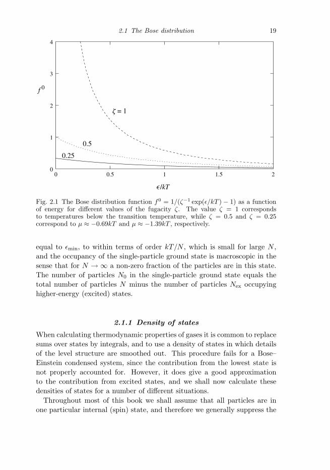
2.1 The Bose distribution 19
Fig. 2.1 The Bose distribution function f0 = 1/(ζ−1 exp(ε/kT ) − 1) as a functionof energy for different values of the fugacity ζ. The value ζ = 1 correspondsto temperatures below the transition temperature, while ζ = 0.5 and ζ = 0.25correspond to μ ≈ −0.69kT and μ ≈ −1.39kT , respectively.
equal to εmin, to within terms of order kT/N , which is small for large N ,and the occupancy of the single-particle ground state is macroscopic in thesense that for N → ∞ a non-zero fraction of the particles are in this state.The number of particles N0 in the single-particle ground state equals thetotal number of particles N minus the number of particles Nex occupyinghigher-energy (excited) states.
2.1.1 Density of states
When calculating thermodynamic properties of gases it is common to replacesums over states by integrals, and to use a density of states in which detailsof the level structure are smoothed out. This procedure fails for a Bose–Einstein condensed system, since the contribution from the lowest state isnot properly accounted for. However, it does give a good approximationto the contribution from excited states, and we shall now calculate thesedensities of states for a number of different situations.
Throughout most of this book we shall assume that all particles are inone particular internal (spin) state, and therefore we generally suppress the

20 The non-interacting Bose gas
part of the wave function referring to the internal state. In Chapters 12, 13,16 and 17 we discuss a number of topics where internal degrees of freedomcome into play.
In three dimensions, for a free particle in a particular internal state, thereis on average one quantum state per volume (2π�)3 of phase space. Theregion of momentum space for which the magnitude of the momentum isless than p has a volume 4πp3/3 equal to that of a sphere of radius p and,since the energy of a particle of momentum p is εp = p2/2m, the totalnumber of states G(ε) with energy less than ε is given by
G(ε) = V4π
3(2mε)3/2
(2π�)3= V
21/2
3π2
(mε)3/2
�3, (2.3)
where V is the volume of the system. Quite generally, the number of stateswith energy between ε and ε+dε is given by g(ε)dε, where g(ε) is the densityof states. Therefore
g(ε) =dG(ε)
dε, (2.4)
which, from Eq. (2.3), is thus
g(ε) =V m3/2
21/2π2�3ε1/2. (2.5)
For a free particle in d dimensions the corresponding result is g(ε) ∝ ε(d/2−1),and therefore the density of states is independent of energy for a free particlein two dimensions.
Let us now consider a particle in the anisotropic harmonic-oscillator po-tential
V (r) =12(Kxx2 + Kyy
2 + Kzz2), (2.6)
which we will refer to as a harmonic trap. Here the quantities Ki (i =x, y, z) denote the three force constants, which are generally unequal. Thecorresponding classical oscillation frequencies ωi are given by ω2
i = Ki/m,and we shall therefore write the potential as
V (r) =12m(ω2
xx2 + ω2yy
2 + ω2zz
2). (2.7)
The energy levels, ε(nx, ny, nz), are then
ε(nx, ny, nz) = (nx +12)�ωx + (ny +
12)�ωy + (nz +
12)�ωz, (2.8)
where the numbers ni assume all integer values greater than or equal tozero.

2.2 Transition temperature and condensate fraction 21
We now determine the number of states G(ε) with energy less than agiven value ε. For energies large compared with �ωi, we may treat the ni
as continuous variables and neglect the zero-point motion. We thereforeintroduce a coordinate system defined by the three variables εi = �ωini, interms of which a surface of constant energy (2.8) is the plane ε = εx+εy +εz.Then G(ε) is proportional to the volume in the first octant bounded by theplane,
G(ε) =1
�3ωxωyωz
∫ ε
0dεx
∫ ε−εx
0dεy
∫ ε−εx−εy
0dεz =
ε3
6�3ωxωyωz. (2.9)
Since g(ε) = dG/dε, we obtain a density of states given by
g(ε) =ε2
2�3ωxωyωz. (2.10)
For a d-dimensional harmonic-oscillator potential with frequencies ωi, theanalogous result is
g(ε) =εd−1
(d − 1)!∏
i �ωi. (2.11)
We thus see that in many contexts the density of states varies as a powerof the energy, and we shall now calculate thermodynamic properties forsystems with a density of states of the form
g(ε) = Cαεα−1, (2.12)
where Cα is a constant. In three dimensions, for a gas confined by rigidwalls, α is equal to 3/2. The corresponding coefficient may be read off fromEq. (2.5), and it is
C3/2 =V m3/2
21/2π2�3. (2.13)
The coefficient for a three-dimensional harmonic-oscillator potential (α = 3),which may be obtained from Eq. (2.10), is
C3 =1
2�3ωxωyωz. (2.14)
2.2 Transition temperature and condensate fraction
The transition temperature Tc is defined as the highest temperature at whichthe macroscopic occupation of the lowest-energy state appears. When thenumber of particles, N , is sufficiently large, we may neglect the zero-pointenergy in (2.8) and thus equate the lowest energy εmin to zero, the minimum
22 The non-interacting Bose gas
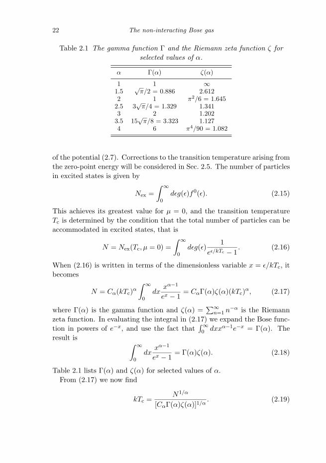
Table 2.1 The gamma function Γ and the Riemann zeta function ζ forselected values of α.
α Γ(α) ζ(α)
1 1 ∞1.5
√π/2 = 0.886 2.612
2 1 π2/6 = 1.6452.5 3
√π/4 = 1.329 1.341
3 2 1.2023.5 15
√π/8 = 3.323 1.127
4 6 π4/90 = 1.082
of the potential (2.7). Corrections to the transition temperature arising fromthe zero-point energy will be considered in Sec. 2.5. The number of particlesin excited states is given by
Nex =∫ ∞
0dεg(ε)f0(ε). (2.15)
This achieves its greatest value for μ = 0, and the transition temperatureTc is determined by the condition that the total number of particles can beaccommodated in excited states, that is
N = Nex(Tc, μ = 0) =∫ ∞
0dεg(ε)
1eε/kTc − 1
. (2.16)
When (2.16) is written in terms of the dimensionless variable x = ε/kTc, itbecomes
N = Cα(kTc)α
∫ ∞
0dx
xα−1
ex − 1= CαΓ(α)ζ(α)(kTc)α, (2.17)
where Γ(α) is the gamma function and ζ(α) =∑∞
n=1 n−α is the Riemannzeta function. In evaluating the integral in (2.17) we expand the Bose func-tion in powers of e−x, and use the fact that
∫∞0 dxxα−1e−x = Γ(α). The
result is ∫ ∞
0dx
xα−1
ex − 1= Γ(α)ζ(α). (2.18)
Table 2.1 lists Γ(α) and ζ(α) for selected values of α.From (2.17) we now find
kTc =N1/α
[CαΓ(α)ζ(α)]1/α. (2.19)

2.2 Transition temperature and condensate fraction 23
For a three-dimensional harmonic-oscillator potential, α is 3 and C3 is givenby Eq. (2.14). From (2.19) we then obtain a transition temperature givenby
kTc =�ωN1/3
[ζ(3)]1/3≈ 0.94�ωN1/3, (2.20)
where
ω = (ωxωyωz)1/3 (2.21)
is the geometric mean of the three oscillator frequencies. The result (2.20)may be written in the useful form
Tc ≈ 4.5(
f
100 Hz
)N1/3 nK, (2.22)
where f = ω/2π.For a uniform Bose gas in a three-dimensional box of volume V the index
α is 3/2. Using the expression (2.13) for the coefficient C3/2, one finds forthe transition temperature the relation
kTc =2π
[ζ(3/2)]2/3
�2n2/3
m≈ 3.31
�2n2/3
m, (2.23)
where n = N/V is the number density. For a uniform gas in two dimensions,α is equal to 1, and the integral in (2.17) diverges. Thus Bose–Einsteincondensation in a two-dimensional box can occur only at zero temperature.However, a two-dimensional Bose gas can condense at non-zero temperatureif the particles are confined by a harmonic-oscillator potential. In that caseα = 2 and the integral in (2.17) is finite. We shall return to gases in lowerdimensions in Chapter 15.
It is useful to introduce the phase-space density, which we denote by .This is defined as the number of particles contained within a volume equalto the cube of the thermal de Broglie wavelength, λ3
T = (2π�2/mkT )3/2,
= n
(2π�
2
mkT
)3/2
. (2.24)
If the gas is classical, this is a measure of the typical occupancy of single-particle states. The majority of occupied states have energies of order kT
or less, and therefore the number of states per unit volume that are oc-cupied significantly is of order the total number of states per unit volumewith energies less than kT , which is approximately (mkT/�
2)3/2 accordingto (2.3). The phase-space density is thus the ratio between the particledensity and the number of significantly occupied states per unit volume.

24 The non-interacting Bose gas
The Bose–Einstein phase transition occurs when = ζ(3/2) ≈ 2.612, ac-cording to (2.23). The criterion that should be comparable with unityindicates that low temperatures and/or high particle densities are necessaryfor condensation.
The existence of a well-defined phase transition for particles in a harmonic-oscillator potential is a consequence of our assumption that the separation ofsingle-particle energy levels is much less than kT . For an isotropic harmonicoscillator, with ωx = ωy = ωz = ω0, this implies that the energy quantum�ω0 should be much less than kTc. Since Tc is given by Eq. (2.20), thecondition is N1/3 1. If the finiteness of the particle number is taken intoaccount, the transition becomes smooth.
2.2.1 Condensate fraction
Below the transition temperature the number Nex of particles in excitedstates is given by Eq. (2.15) with μ = 0,
Nex(T ) = Cα
∫ ∞
0dεεα−1 1
eε/kT − 1. (2.25)
Provided the integral converges, that is α > 1, we may use Eq. (2.18) towrite this result as
Nex = CαΓ(α)ζ(α)(kT )α. (2.26)
Note that this result does not depend on the total number of particles.However, if one makes use of the expression (2.19) for Tc, it may be rewrittenin the form
Nex = N
(T
Tc
)α
. (2.27)
The number of particles in the condensate is thus given by
N0(T ) = N − Nex(T ) (2.28)
or
N0 = N
[1 −(
T
Tc
)α]. (2.29)
For particles in a box in three dimensions, α is 3/2, and the number ofexcited particles per unit volume, nex, may be obtained from Eqs. (2.26)and (2.13). It is
nex =Nex
V= ζ(3/2)
(mkT
2π�2
)3/2
. (2.30)

2.3 Density profile and velocity distribution 25
The occupancy of the condensate is therefore given by the well-known resultN0 = N [1 − (T/Tc)3/2].
For a three-dimensional harmonic-oscillator potential (α = 3), the numberof particles in the condensate is
N0 = N
[1 −(
T
Tc
)3]. (2.31)
In all cases the transition temperature Tc is given by (2.19) for the appro-priate value of α.
2.3 Density profile and velocity distribution
The cold clouds of atoms investigated at microkelvin temperatures typicallycontain of order 104–108 atoms. It is not feasible to apply the usual tech-niques of low-temperature physics to these systems for a number of reasons.First, there are rather few atoms, second, the systems are metastable, so onecannot allow them to come into equilibrium with another body, and third,the systems have a lifetime which is of order seconds to minutes.
Among the quantities that can be measured is the density profile. Oneway to do this is by absorptive imaging. Light at a resonant frequencyfor the atom will be absorbed on passing through an atomic cloud. Thusby measuring the absorption profile one can obtain information about thedensity distribution. The spatial resolution can be improved by switchingoff the trap, thereby allowing the cloud to expand before measuring theabsorption. The expansion also overcomes a difficulty that many trappedcold-gas clouds absorb so strongly on resonance that an absorptive imageyields little information. A drawback of absorptive imaging is that it isdestructive, since absorption of light changes the internal states of atomsand heats the cloud significantly. In addition, in the case of imaging afterexpansion, study of time-dependent phenomena requires preparation of anew cloud for each time point. An alternative technique is to use phase-contrast imaging [2,3]. This exploits the fact that the refractive index of thegas depends on its density, and therefore the optical path length is changedby the medium. By allowing a light beam that has passed through the cloudto interfere with a reference beam that has been phase shifted, changesin optical path length may be converted into intensity variations, just asin phase-contrast microscopy. The advantage of this method is that it isalmost non-destructive, and it is therefore possible to study time-dependentphenomena using a single cloud.
In the ground state of the system, all atoms are condensed in the lowest

26 The non-interacting Bose gas
single-particle quantum state and the density distribution n(r) reflects theshape of the ground-state wave function φ0(r) for a particle in the trap since,for non-interacting particles, the density is given by
n(r) = N |φ0(r)|2, (2.32)
where N is the number of particles. For an anisotropic harmonic oscillatorthe ground-state wave function is
φ0(r) =1
π3/4(axayaz)1/2e−x2/2a2
xe−y2/2a2ye−z2/2a2
z , (2.33)
where the widths ai of the wave function in the three directions (i = x, y, z)are given by
a2i =
�
mωi. (2.34)
The density distribution is thus anisotropic if the three frequencies ωx, ωy
and ωz are not all equal, the greatest width being associated with the lowestfrequency. The widths ai may be written in a form analogous to (2.22)
ai ≈ 10.1(
100 Hzfi
1A
)1/2
μm, (2.35)
in terms of the trap frequencies fi = ωi/2π and the mass number A, thenumber of nucleons in the nucleus of the atom.
The distribution of particles after a cloud is allowed to expand dependsnot only on the initial density distribution, but also on the initial velocitydistribution. Consequently it is important to consider the velocity distri-bution. In momentum space the wave function corresponding to (2.33) isobtained by taking its Fourier transform and is
φ0(p) =1
π3/4(cxcycz)1/2e−p2
x/2c2xe−p2y/2c2ye−p2
z/2c2z , (2.36)
where
ci =�
ai=√
m�ωi. (2.37)
Thus the density in momentum space is given by
n(p) = N |φ0(p)|2 =N
π3/2cxcycze−p2
x/c2xe−p2y/c2ye−p2
z/c2z . (2.38)
Since c2i /m = �ωi, the distribution (2.38) has the form of a Maxwell distri-
bution with different ‘temperatures’ Ti = �ωi/2k for the three directions.Since the spatial distribution is anisotropic, the momentum distribution

2.3 Density profile and velocity distribution 27
also depends on direction. By the Heisenberg uncertainty principle, a narrowspatial distribution implies a broad momentum distribution, as seen in theFourier transform (2.36) where the widths ci are proportional to the squareroot of the oscillator frequencies.
These density and momentum distributions may be contrasted with thecorresponding expressions when the gas obeys classical statistics, at temper-atures well above the Bose–Einstein condensation temperature. The densitydistribution is then proportional to exp[−V (r)/kT ] and consequently it isgiven by
n(r) =N
π3/2RxRyRze−x2/R2
xe−y2/R2ye−z2/R2
z . (2.39)
Here the widths Ri are given by
R2i =
2kT
mω2i
, (2.40)
and they therefore depend on temperature. Note that the ratio Ri/ai equals(2kT/�ωi)1/2, which under typical experimental conditions is much greaterthan unity. Consequently the condition for semi-classical behaviour is wellsatisfied, and one concludes that the thermal cloud is much broader thanthe condensate, which below Tc emerges as a narrow peak in the spatialdistribution with a weight that increases with decreasing temperature.
Above Tc the density n(p) in momentum space is isotropic in equilibrium,since it is determined only by the temperature and the particle mass, andin the classical limit it is given by
n(p) = Ce−p2/2mkT , (2.41)
where the constant C is independent of momentum. The width of the mo-mentum distribution is thus ∼ (mkT )1/2, which is ∼ (kT/�ωi)1/2 timesthe zero-temperature width (m�ωi)1/2. At temperatures comparable withthe transition temperature one has kT ∼ N1/3
�ωi and therefore the factor(kT/�ωi)1/2 is of the order of N1/6. The density and velocity distributionsof the thermal cloud are thus much broader than those of the condensate.
If a thermal cloud is allowed to expand to a size much greater than itsoriginal one, the resulting cloud will be spherically symmetric due to theisotropy of the velocity distribution, as we shall demonstrate explicitly inSec. 2.3.1 below. This is quite different from the anisotropic shape of an ex-panding cloud of condensate. In early experiments the anisotropy of cloudsafter expansion provided strong evidence for the existence of a Bose–Einsteincondensate.

28 The non-interacting Bose gas
Interactions between the atoms alter the sizes of clouds somewhat, as weshall see in Sec. 6.2. A repulsive interaction increases the size of a zero-temperature condensate cloud in equilibrium by a numerical factor whichdepends on the number of particles and the interatomic potential, typicalvalues being in the range between 2 and 10, while an attractive interactioncan cause the cloud to collapse. Above Tc, where the cloud is less dense,interactions hardly affect the size of the cloud.
2.3.1 The semi-classical distribution
Quantum-mechanically, the density of non-interacting bosons is given by
n(r) =∑
ν
fν |φν(r)|2, (2.42)
where fν is the occupation number for state ν, for which the wave function isφν(r). Such a description is unwieldy in general, since it demands a knowl-edge of the wave functions for the trapping potential in question. However,provided the de Broglie wavelengths of particles are small compared with thelength scale over which the trapping potential varies significantly, a simplerdescription is possible as we shall see in the following.
Classically, the state of a particle is determined by specifying its positionr and its momentum p, which implies that the statistical properties of a gasmay be expressed in terms of a distribution function depending on r and p.According to the Heisenberg uncertainty principle, in quantum mechanicsthe momentum and position of a particle cannot be specified with arbitraryaccuracy, and therefore such a description is in general not possible. How-ever, provided properties of interest do not require information about theparticle distribution on length scales Δl and momentum scales Δp that vio-late the uncertainty relation ΔlΔp ≥ �/2, a simpler description of the systemis possible in terms of a semi-classical distribution function fp(r) represent-ing the average occupancy of a quantum state. Semi-classically, the numberof quantum states with momenta lying within the volume element dpdr inphase space is dpdr/(2π�)3, and therefore the quantity fp(r)dpdr/(2π�)3 isthe mean number of particles in the phase space volume dpdr. For such adescription to be applicable, it is necessary that the characteristic distanceover which the momentum of a particle changes is large compared with thede Broglie wavelength of the particle.
The physical content of this approximation is that locally the gas may beregarded as having the same properties as a bulk gas. We have used thisapproximation to discuss the high-temperature limit of Boltzmann statistics,

2.3 Density profile and velocity distribution 29
but it may also be used under conditions when the gas is degenerate. Thedistribution function in equilibrium is therefore given by
fp(r) = f0p(r) =
1e[εp(r)−μ]/kT − 1
. (2.43)
Here the particle energies are those of a classical free particle at point r,
εp(r) =p2
2m+ V (r), (2.44)
where V (r) is the external potential.This description may be used for particles in excited states, but it is inap-
propriate for the ground state, which has spatial variations on length scalescomparable with those over which the trap potential varies significantly.Also, calculating properties of the system by integrating over momentumstates does not properly take into account the condensed state, but prop-erties of particles in excited states are well estimated by the semi-classicalresult. Thus, for example, to determine the number of particles in excitedstates, one integrates the semi-classical distribution function (2.43) dividedby (2π�)3 over p and r. The results for Tc agree with those obtained by themethods described in Sec. 2.2 above, where the effect of the potential wasincluded through the density of states. To demonstrate this for a harmonictrap is left as an exercise (Problem 2.1).
We now consider the density of particles which are not in the condensate.This is given by
nex(r) =∫
dp(2π�)3
1e[εp(r)−μ]/kT − 1
. (2.45)
We evaluate the integral (2.45) by introducing the variable x = p2/2mkT
and the quantity z(r) defined by the equation
z(r) = e[μ−V (r)]/kT . (2.46)
For V (r) = 0, z reduces to the fugacity. One finds
nex(r) =2√πλ3
T
∫ ∞
0dx
x1/2
z−1ex − 1, (2.47)
where λT = (2π�2/mkT )1/2 is the thermal de Broglie wavelength, Eq. (1.2).
Integrals of this type occur frequently in expressions for properties of idealBose gases, so we shall consider a more general one. They are evaluated byexpanding the integrand in powers of z, and one finds∫ ∞
0dx
xγ−1
z−1ex − 1=
∞∑n=1
∫ ∞
0dxxγ−1e−nxzn = Γ(γ)gγ [z], (2.48)

30 The non-interacting Bose gas
Fig. 2.2 The spatial distribution of non-condensed particles, Eq. (2.50), for anisotropic trap, V (r) = mω2
0r2/2, with R = (2kT/mω20)1/2. The dotted line is a
Gaussian distribution, corresponding to the first term in the sum (2.49).
where
gγ [z] =∞∑
n=1
zn
nγ. (2.49)
For z = 1, the sum in (2.49) reduces to ζ(γ), in agreement with (2.18).The integral in (2.47) corresponds to γ = 3/2, and therefore
nex(r) =g3/2[z(r)]
λ3T
. (2.50)
In Fig. 2.2 we show for a harmonic trap the density of excited particles inunits of 1/λ3
T for a chemical potential equal to the minimum of the potential.This gives the distribution of excited particles at the transition temperatureor below. For comparison the result for the classical Boltzmann distribution,which corresponds to the first term in the series (2.49), is also exhibited forthe same value of μ. In the semi-classical approximation the density hasa sharp peak at the origin, with dn/dr → constant, whereas in a moreprecise treatment the peak is smoothed over a length scale of order λT .For a harmonic trap above the transition temperature, the total number of

2.3 Density profile and velocity distribution 31
particles is related to the chemical potential by
N = g3[z(0)](
kT
�ω
)3
, (2.51)
as one can verify by integrating (2.45) over space.
Free expansion
As mentioned above, the observed anisotropy of a cloud after expansionprovides evidence for the existence of a Bose–Einstein condensate. In orderto illustrate this, we consider in the following the free expansion of a cloudof non-interacting particles, which are initially trapped in an anisotropicharmonic-oscillator potential. For simplicity, we shall contrast the behaviourof a pure condensate with that of a classical gas at temperatures well aboveits transition temperature Tc, but the treatment given below may be readilygeneralized to the case when T ≥ Tc.
In the classical limit, the distribution function (2.43) in equilibrium is
f0p(r) = eμ/kT e−εp(r)/kT . (2.52)
The initial distribution, before the potential is turned off and the gas al-lowed to expand freely, is thus (2.52) where the energies εp(r) are given by(2.44) and (2.7). When the gas expands freely, the individual particles moveaccording to the equations of motion
r = p/m; p = 0, (2.53)
where the dot denotes a time derivative. During the free expansion, inthe absence of collisions the distribution function remains unchanged whenone follows the motion of an individual particle, according to the Liouvilletheorem. If the time at which the potential is turned off is taken to be t = 0,the distribution at later times is therefore given by
fp(r, t) = f0p(r − pt/m) = eμ/kT e−[p2/2m+V (r−pt/m)]/kT , (2.54)
and the density n(r, t) is obtained by integrating over momentum,
n(r, t) =∫
dp(2π�)3
fp(r, t). (2.55)
The integral may be evaluated by performing the integration over each mo-mentum component pi separately and shifting the origin on each pi axis to

32 The non-interacting Bose gas
obtain simple Gaussian integrals, and the result is
n(r, t) = eμ/kT 1λ3
T
∏i
(1 + ω2i t
2)−1/2e−mω2i r2
i /2kT (1+ω2i t2), (2.56)
where ri = x, y, z. At time t = 0 this agrees with (2.50) and (2.39), since inthe classical limit g3/2[z(r)] � z(r). The anisotropy of the initial distributionis thus determined by the oscillator frequencies, as shown in (2.39). At timesmuch larger than 1/ωi, however, the density distribution (2.56) becomesisotropic, with a width given by the thermal velocity (2kT/m)1/2 times t.
Let us now consider the expansion of a Bose–Einstein condensed cloudat zero temperature, where the single-particle wave function at t = 0 isgiven in momentum space by (2.36). At later times, the wave functiondevelops according to the Schrodinger equation for a free particle, whichimplies that the wave function in momentum space is simply given by (2.36)times exp(−ip2t/2m�). The wave function φ(r, t) in real space is thereforeobtained from
φ(r, t) =∫
dp(2π�)3/2
φ0(p)e−ip2t/2m�eip·r/�. (2.57)
The integration may be carried out as described just below Eq. (2.55) andone finds
φ(r, t) =1
π3/4
∏i
a−1/2i (1 + iωit)−1/2e−r2
i /[2a2i (1+iωit)]. (2.58)
The anisotropy of the density, which is proportional to |φ(r, t)|2, thuschanges dramatically upon expansion. At t = 0 the width of the cloudin the i direction is given by ai = (�/mωi)1/2, while at large times the widthis aiωit = (�ωi/m)1/2t in the i direction. A cigar-shaped Bose–Einsteincondensed cloud thus becomes pancake-like upon expansion.
This qualitative conclusion holds also when interactions between atomsbecome important, as will be discussed in greater detail in Sec. 7.5. Inthat case expansion of the cloud is a result of the force due to the pressuregradient produced by the interaction, rather than to the velocity componentspresent in the initial cloud. The pressure due to interactions is a function ofthe local particle density, and therefore its gradient is greater in directionsin which the cloud extension is smallest. Consequently, the acceleration andthe final velocity of atoms are greatest in directions in which the initial cloudwas most compact.

2.4 Thermodynamic quantities 33
2.4 Thermodynamic quantities
In this section we determine thermodynamic properties of ideal Bose gasesand calculate the energy, entropy, and other properties of the condensedphase. We explore how the temperature dependence of the specific heatfor temperatures close to Tc depends on the parameter α characterizing thedensity of states.
2.4.1 Condensed phase
The energy of the macroscopically occupied state is taken to be zero, andtherefore only excited states contribute to the total energy of the system.Consequently in converting sums to integrals it is not necessary to include anexplicit term for the condensate, as it is when calculating the total numberof particles. Below Tc, the chemical potential vanishes, and the internalenergy is given by
E = Cα
∫ ∞
0dεεα−1 ε
eε/kT − 1= CαΓ(α + 1)ζ(α + 1)(kT )α+1, (2.59)
where we have used the integral (2.18). The specific heat C = ∂E/∂T istherefore given by1
C = (α + 1)E
T. (2.60)
Since the specific heat is also given in terms of the entropy S by C =T∂S/∂T , we find
S =C
α=
α + 1α
E
T. (2.61)
Note that below Tc the energy, entropy, and specific heat do not depend onthe total number of particles. This is because only particles in excited statescontribute, and consequently the number of particles in the macroscopicallyoccupied state is irrelevant for these quantities.
Expressed in terms of the total number of particles N and the transitiontemperature Tc, which are related by Eq. (2.19), the energy is given by
E = Nkαζ(α + 1)
ζ(α)Tα+1
Tαc
, (2.62)
where we have used the property of the gamma function that Γ(z + 1) =
1 The specific heat C is the temperature derivative of the internal energy, subject to the conditionthat the trap parameters are unchanged. For particles in a box, C is thus the specific heat atconstant volume.
34 The non-interacting Bose gas
zΓ(z). As a consequence, the specific heat is given by
C = α(α + 1)ζ(α + 1)
ζ(α)Nk
(T
Tc
)α
, (2.63)
while the entropy is
S = (α + 1)ζ(α + 1)
ζ(α)Nk
(T
Tc
)α
. (2.64)
Let us compare the results above with those in the classical limit. At hightemperatures, the Bose–Einstein distribution becomes a Boltzmann distri-bution, and therefore
N = Cα
∫ ∞
0dεεα−1e(μ−ε)/kT (2.65)
and
E = Cα
∫ ∞
0dεεαe(μ−ε)/kT . (2.66)
On integrating Eq. (2.66) by parts, we obtain
E = αNkT, (2.67)
which implies that the high-temperature specific heat is
C = αNk. (2.68)
For a homogeneous gas in three dimensions, for which α = 3/2, the result(2.68) is C = 3Nk/2, and for a harmonic-oscillator potential in three dimen-sions C = 3Nk. Both these results are in agreement with the equipartitiontheorem. The ratio of the specific heat in the condensed state to its valuein the classical limit is thus given by
C(T )αNk
= (α + 1)ζ(α + 1)
ζ(α)
(T
Tc
)α
. (2.69)
At Tc the ratio is approximately 1.28 for a uniform gas in three dimensions(α = 3/2), and 3.60 for a three-dimensional harmonic-oscillator potential(α = 3).
For later applications we shall require explicit expressions for the pressureand entropy of a homogeneous Bose gas. For an ideal gas in three dimen-sions, the pressure is given by p = 2E/3V , irrespective of statistics. Forthe condensed Bose gas this result may be derived by using the fact that

2.4 Thermodynamic quantities 35
p = −(∂E/∂V )S , with the energy given by (2.62) for α = 3/2. Accordingto Eq. (2.23) Tc scales as n2/3, and one finds
p = nkζ(5/2)ζ(3/2)
T 5/2
T3/2c
= ζ(5/2)( m
2π�2
)3/2(kT )5/2. (2.70)
From Eq. (2.64), the entropy per particle is seen to be
S
N= k
52
ζ(5/2)ζ(3/2)
(T
Tc
)3/2
. (2.71)
These results will be used in the discussion of sound modes in Sec. 10.4.
2.4.2 Normal phase
Let us now consider the leading corrections to the classical result (2.68) forthe specific heat. The general expression for the total number of particles is
N = Cα
∫ ∞
0dεεα−1 1
e(ε−μ)/kT − 1, (2.72)
while that for the total energy is
E = Cα
∫ ∞
0dεεα 1
e(ε−μ)/kT − 1. (2.73)
At high temperatures the mean occupation numbers are small. We maytherefore use in these two equations the expansion (ex − 1)−1 � e−x + e−2x
valid for large x, and obtain
N � Cα
∫ ∞
0dεεα−1[e(μ−ε)/kT + e2(μ−ε)/kT ] (2.74)
and
E � Cα
∫ ∞
0dεεα[e(μ−ε)/kT + e2(μ−ε)/kT ], (2.75)
from which we may eliminate the chemical potential μ by solving (2.74) forexp(μ/kT ) and inserting the result in (2.75). This yields
E
αNkT� 1 − ζ(α)
2α+1
(Tc
T
)α
, (2.76)
where we have used (2.19) to express N/Cα in terms of Tc. The specific heatis then given by
C � αNk
[1 + (α − 1)
ζ(α)2α+1
(Tc
T
)α]. (2.77)

36 The non-interacting Bose gas
This approximate form is useful even at temperatures only slightly above Tc.The expressions (2.72) and (2.73) may be applied to non-interacting
fermions as well, by replacing the Bose–Einstein distribution function bythe Fermi–Dirac one, that is by changing −1 in the denominator to +1. Asa consequence, for fermions the leading corrections to the classical resultsat high temperature have the opposite sign from those for bosons. The en-ergy of a Fermi gas exceeds the classical result, a direct manifestation of theexclusion principle. We shall return to the properties of fermion clouds inChapter 16.
2.4.3 Specific heat close to Tc
Having calculated the specific heat at high temperatures and at tempera-tures less than Tc we now determine its behaviour near Tc. We shall seethat it exhibits a discontinuity at Tc if α exceeds 2. By contrast, for auniform Bose gas (for which α equals 3/2) the specific heat at constant vol-ume is continuous at Tc, but its derivative with respect to temperature isdiscontinuous.
We shall consider the energy E as a function of the two variables T andμ. These are constrained by the condition that the total number of particlesbe equal to N . The change in energy, δE, may then be written as δE =(∂E/∂T )μδT + (∂E/∂μ)T δμ. The term proportional to δT is the same justabove and just below the transition, and therefore it gives contributionsto the specific heat that are continuous at Tc. The source of the singularbehaviour is the term proportional to δμ, since the chemical potential μ isidentically zero for temperatures less than Tc and becomes non-zero (in fact,negative) above the transition. To determine the nature of the singularity itis sufficient to consider temperatures just above Tc, and evaluate the change(from zero) of the chemical potential, δμ, to lowest order in T − Tc. Thenon-zero value δμ of the chemical potential results in a contribution to theinternal energy given by (∂E/∂μ)δμ. The derivative may be calculated bytaking the derivative of Eq. (2.73) and integrating by parts, and one finds∂E/∂μ = αN . The discontinuity in the specific heat is therefore
ΔC = C(Tc+) − C(Tc−) = αN∂μ
∂T
∣∣∣∣T=Tc+
, (2.78)
where the derivative is to be evaluated for fixed particle number.We determine the dependence of μ on T just above Tc by calculating the

2.4 Thermodynamic quantities 37
Fig. 2.3 The specific heat C, in units of αNk, as a function of the reduced temper-ature T/Tc for different values of α.
derivative (∂μ/∂T )N , using the identity(∂μ
∂T
)N
= −(
∂μ
∂N
)T
(∂N
∂T
)μ
= −(
∂N
∂T
)μ
(∂N
∂μ
)−1
T
, (2.79)
which follows from the fact that
dN =(
∂N
∂T
)μ
dT +(
∂N
∂μ
)T
dμ = 0 (2.80)
when the particle number is fixed. The derivatives are evaluated by differ-entiating the expression (2.72) which applies at temperatures at or above Tc
and integrating by parts. The results at Tc are(∂N
∂μ
)T
=ζ(α − 1)
ζ(α)N
kTc(2.81)
and (∂N
∂T
)μ
= αN
Tc, (2.82)
which yield (∂μ
∂T
)N
= −αζ(α)
ζ(α − 1)k. (2.83)

38 The non-interacting Bose gas
We have assumed that α is greater than 2, since otherwise the expansion isnot valid.
For T − Tc Tc this yields
μ � −αζ(α)
ζ(α − 1)k(T − Tc), (2.84)
which, when inserted into Eq. (2.78), gives the specific heat discontinuity
ΔC = −α2 ζ(α)ζ(α − 1)
Nk. (2.85)
For a harmonic-oscillator potential, corresponding to α = 3, the jump in thespecific heat is
ΔC = −9ζ(3)ζ(2)
Nk ≈ −6.58Nk. (2.86)
For α ≤ 2, the expansion given above is not permissible, and the in-vestigation of the specific heat for that case is the subject of Problem 2.4.We exhibit in Fig. 2.3 the temperature-dependent specific heat for differentvalues of α. Note that the specific heat of an ideal, uniform Bose gas atconstant pressure diverges as the temperature approaches Tc from above(Problem 2.5).
2.5 Effect of finite particle number
For a cloud of N bosons in a three-dimensional harmonic trap the transitiontemperature as given by (2.20) is proportional to N1/3. We now considerthe leading correction to this result due to the finiteness of the number ofparticles. As we shall see, this is independent of N , and is therefore of rela-tive order N−1/3. For a cloud containing 106 atoms it lowers the transitiontemperature by about 1%, while for 104 atoms the effect is somewhat larger,of order 5%.
The correction to Tc originates in the zero-point motion, which increasesthe energy of the lowest single-particle state by an amount (see Eq. (2.8))
Δεmin =�
2(ωx + ωy + ωz) =
3�ωm
2, (2.87)
where
ωm = (ωx + ωy + ωz)/3 (2.88)
is the algebraic mean of the frequencies. Thus the shift in the chemicalpotential at the transition temperature is
Δμ = Δεmin. (2.89)

2.5 Effect of finite particle number 39
To determine the shift ΔTc in the transition temperature for particlestrapped by a three-dimensional harmonic-oscillator potential we use the in-verse of the result (2.83) to relate the shift in transition temperature to thechange in the chemical potential. When condensation sets in, the chemi-cal potential is equal to the expression (2.89) when the zero-point energy istaken into account. Since α = 3 for the three-dimensional harmonic trap,the shift in transition temperature is
ΔTc = − ζ(2)3ζ(3)
Δμ
k= − ζ(2)
2ζ(3)�ωm
k. (2.90)
Inserting Tc from (2.20) we obtain the result
ΔTc
Tc= − ζ(2)
2[ζ(3)]2/3
ωm
ωN−1/3 ≈ −0.73
ωm
ωN−1/3, (2.91)
which shows that the fractional change in the transition temperature isproportional to N−1/3.
For an anisotropic trap with axial symmetry, where ωz = λωx = λωy,the ratio ωm/ω becomes (2 + λ)/3λ1/3. Since λ may be as small as 10−3,anisotropy can enhance significantly the effects of finite particle number.
Since the force constants of the harmonic trapping potential can be var-ied almost at will, it is possible to create very elongated or highly flattenedcondensates and thus explore Bose–Einstein condensation in lower dimen-sions. In a homogeneous system Bose–Einstein condensation cannot takeplace at non-zero temperature in one or two dimensions. This can be seenfrom the discussion in Sec. 2.2 above. For a uniform gas of particles in twodimensions the density of states is independent of energy, and the integral inEq. (2.17) relating the transition temperature to the particle number there-fore does not exist. The situation is different in traps, since the density ofstates for a particle in a two-dimensional harmonic trap is proportional tothe energy. In Chapter 15 we discuss some of the phenomena associatedwith lower-dimensional systems.
Problems
Problem 2.1 Use the semi-classical distribution function (2.43) to calcu-late the number of particles in the condensate for an isotropic harmonic-oscillator potential. Indicate how the calculation may be generalized to ananisotropic harmonic oscillator.
Problem 2.2 Consider a gas of N identical bosons, each of mass m, in

40 The non-interacting Bose gas
the quadrupole trap potential
V (x, y, z) = A(x2 + y2 + 4z2)1/2,
where A is a positive constant (the physics of this trap will be explainedin Sec. 4.1). Use the semi-classical approach to determine the density ofsingle-particle states as a function of energy and calculate the transitiontemperature, the depletion of the condensate as a function of temperature,and the jump in the specific heat at the transition temperature. [Hint: Findthe local density of states and integrate the result over r].
Problem 2.3 Determine the Bose–Einstein condensation temperature andthe temperature dependence of the depletion of the condensate for N iden-tical bosons of mass m in an isotropic potential given by the power lawV (r) = Crν , where C and ν are positive constants.
Problem 2.4 Prove that the discontinuity in the specific heat at Tc, ob-tained in (2.85) for α > 2, disappears when α < 2 by using the identity
N − CαΓ(α)ζ(α)(kT )α = Cα
∫ ∞
0dεεα−1
[1
e(ε−μ)/kT − 1− 1
eε/kT − 1
]
at temperatures just above Tc. [Hint: Simplify the integrand by using theapproximation (ex − 1)−1 � 1/x.]
Problem 2.5 Consider a uniform non-interacting gas of N identicalbosons of mass m in a volume V . Use the method employed in Problem 2.4 tocalculate the chemical potential as a function of temperature and volume attemperatures just above Tc. Show that the specific heat at constant pressure,Cp, diverges as (T −Tc)−1 when the temperature approaches Tc from above.[Hint: The thermodynamic identity Cp = CV − T (∂p/∂T )2V /(∂p/∂V )T maybe useful.]
References[1] L. D. Landau and E. M. Lifshitz, Statistical Physics, Part 1, Third edition,
(Oxford, Pergamon, 1980), §62.[2] M. R. Andrews, M.-O. Mewes, N. J. van Druten, D. S. Durfee, D. M. Kurn,
and W. Ketterle, Science 273, 84 (1996).[3] W. Ketterle, D. S. Durfee, and D. M. Stamper-Kurn, in Bose–Einstein
Condensation in Atomic Gases, Proceedings of the Enrico FermiInternational School of Physics, Vol. CXL, ed. M. Inguscio, S. Stringari, andC. E. Wieman, (Amsterdam, IOS Press, 1999), p. 67.

3
Atomic properties
A number of atomic properties play a key role in experiments on cold atomicgases, and we shall discuss them briefly in the present chapter with particularemphasis on alkali atoms. Basic atomic structure is the subject of Sec. 3.1.Two effects exploited to trap and cool atoms are the influence of a magneticfield on atomic energy levels, and the response of an atom to radiation. InSec. 3.2 we describe the combined influence of the hyperfine interaction andthe Zeeman effect on the energy levels of an atom, and in Sec. 3.3 we reviewthe calculation of the atomic polarizability. In Sec. 3.4 we summarize andcompare some energy scales.
3.1 Atomic structure
The total spin of a Bose particle must be an integer, and therefore a bosonmade up of fermions must contain an even number of them. Neutral atomscontain equal numbers of electrons and protons, and therefore the statisticsthat an atom obeys is determined solely by the number of neutrons N : ifN is even, the atom is a boson, and if it is odd, a fermion. Since the alkalishave odd atomic number Z, boson alkali atoms have odd mass numbers A.Likewise for atoms with even Z, bosonic isotopes have even A. In Table3.1 we list N , Z, and the nuclear spin quantum number I for some alkaliatoms and hydrogen. We also give the nuclear magnetic moment μ, whichis defined as the expectation value of the z component of the magneticmoment operator in the state where the z component of the nuclear spin,denoted by mI�, has its maximum value, μ = 〈I, mI = I|μz|I, mI = I〉.To date, most experiments on Bose–Einstein condensation have been madewith states having total electronic spin 1/2. The majority of these havebeen made with atoms having nuclear spin I = 3/2 (87Rb, 23Na, and 7Li),while others have involved I = 1/2 (H) and I = 5/2 (85Rb). In addition,
41

42 Atomic properties
Table 3.1 The proton number Z, the neutron number N , the nuclear spinI, the nuclear magnetic moment μ (in units of the nuclear magneton
μN = e�/2mp), and the hyperfine splitting νhf = ΔEhf/h for hydrogen andsome alkali isotopes. For completeness, the two fermion isotopes 6Li and
40K are included.
Isotope Z N I μ/μN νhf (MHz)1H 1 0 1/2 2.793 14206Li 3 3 1 0.822 2287Li 3 4 3/2 3.256 80423Na 11 12 3/2 2.218 177239K 19 20 3/2 0.391 46240K 19 21 4 −1.298 −128641K 19 22 3/2 0.215 25485Rb 37 48 5/2 1.353 303687Rb 37 50 3/2 2.751 6835133Cs 55 78 7/2 2.579 9193
Bose–Einstein condensation has been achieved for four species with othervalues of the electronic spin, and nuclear spin I = 0: 4He* (4He atoms inthe lowest electronic triplet state, which is metastable) which has S = 1,170Yb and 174Yb (S = 0), and 52Cr (S = 3).
The ground-state electronic structure of alkali atoms is simple: all elec-trons but one occupy closed shells, and the remaining one is in an s orbital ina higher shell. In Table 3.2 we list the ground-state electronic configurationsfor alkali atoms. The nuclear spin is coupled to the electronic spin by thehyperfine interaction. Since the electrons have no orbital angular momen-tum (L = 0), there is no magnetic field at the nucleus due to the orbitalmotion, and the coupling arises solely due to the magnetic field producedby the electronic spin. The coupling of the electronic spin, S = 1/2, tothe nuclear spin I yields the two possibilities F = I ± 1/2 for the quantumnumber F for the total spin, according to the usual rules for addition ofangular momentum.
In the absence of an external magnetic field the atomic levels are split bythe hyperfine interaction. The coupling is represented by a term Hhf in theHamiltonian of the form
Hhf = AI·J, (3.1)
where A is a constant, while I and J are the operators for the nuclear spinand the electronic angular momentum, respectively, in units of �. For the

3.1 Atomic structure 43
Table 3.2 The electron configuration and electronic spin for selected alkaliatoms and hydrogen. For clarity, the inner-shell configurations for Rb andCs are given in terms of those for the noble gases Ar, 1s22s22p63s23p6, and
Kr, (Ar)3d104s24p6.
Element Z Electronic spin Electron configuration
H 1 1/2 1sLi 3 1/2 1s22s1Na 11 1/2 1s22s22p63s1K 19 1/2 1s22s22p63s23p64s1Rb 37 1/2 (Ar)3d104s24p65s1Cs 55 1/2 (Kr)4d105s25p66s1
atoms other than the alkalis and hydrogen that have been Bose–Einsteincondensed there is no hyperfine splitting, since I = 0 for 4He*, 52Cr, 170Yband 174Yb. The operator for the total angular momentum is equal to
F = I + J. (3.2)
By squaring this expression we may express I·J in terms of the quantumnumbers I, J , and F determining the squares of the angular momentumoperators and the result is
I·J =12
[F (F + 1) − I(I + 1) − J(J + 1)]. (3.3)
Alkali and hydrogen atoms in their ground states have J = S = 1/2. Thesplitting between the levels F = I + 1/2 and F = I − 1/2 is therefore givenby
ΔEhf = hνhf =(
I +12
)A. (3.4)
Measured values of the hyperfine splitting are given in Table 3.1.As a specific example, consider an alkali atom with I = 3/2 in its ground
state (J = S = 1/2). The quantum number F may be either 1 or 2,and I·J = −5/4 and 3/4, respectively. The corresponding shifts of theground-state multiplet are given by E1 = −5A/4 (three-fold degenerate) andE2 = 3A/4 (five-fold degenerate). The energy difference ΔEhf = E2 − E1
due to the hyperfine interaction (3.1) is thus
ΔEhf = 2A, (3.5)
in agreement with the general expression (3.4).

44 Atomic properties
A first-order perturbation treatment of the magnetic dipole–dipole inter-action between the outermost s electron and the nucleus yields the expres-sion [1, §121]
ΔEhf =μ0
4π
16π
3μBμ
(I + 1/2)I
|ψ(0)|2. (3.6)
The quantity μB = e�/2me (the Bohr magneton) is the magnitude of themagnetic moment of the electron with radiative corrections omitted, andμ is the magnetic moment of the nucleus, which is of order the nuclearmagneton μN = e�/2mp = (me/mp)μB. Here me is the electron mass andmp the proton mass. Throughout we denote the elementary charge, theabsolute value of the charge of the electron, by e. The quantity ψ(0) is thevalence s-electron wave function at the nucleus. It follows from Eq. (3.6)that for atoms with a positive nuclear magnetic moment, which is the casefor all the alkali isotopes listed in Table 3.1 except 40K, the state with lowestenergy has F = I − 1/2. For negative nuclear magnetic moment the statewith F = I + 1/2 has the lower energy.
Let us compare the frequency of the hyperfine line in hydrogen with theexpression (3.6). For hydrogen, μ is the proton magnetic moment μp ≈2.793μN and |ψ(0)|2 = 1/πa3
0, where a0 = �2/mee
20 is the Bohr radius, with
e20 = e2/4πε0. Thus (3.6) becomes
ΔEhf =323
μ0
4π
μBμp
a30
. (3.7)
The magnitude of ΔEhf is of order (me/mp)αfs in atomic units (a.u.), whereαfs = e2
0/�c, c being the velocity of light, is the fine structure constant andthe atomic unit of energy is e2
0/a0. The calculated result (3.7) differs fromthe experimental one by less than 1%.
Transitions between hyperfine states are important for applications inother contexts. The hyperfine transition for the hydrogen atom, which hasa frequency of 1420 MHz, is the famous 21-cm line exploited by radio as-tronomers, while the frequency for the transition in the ground state of Csdefines the time standard.
For monovalent multi-electron atoms, Eq. (3.6) shows that the hyperfinesplitting is proportional to the electron density at the nucleus due to thevalence electron. If interactions between electrons could be neglected, theelectron orbitals would be hydrogenic, and the hyperfine interaction wouldscale as (Z/n)3, where n is the principal quantum number for the outermosts electron. However, due to screening by electrons in the atomic core, thepotential seen by the valence electron is not Coulombic, and the characteris-
3.2 The Zeeman effect 45
tic valence electron density at the nucleus varies as ∼ Z, a fact that may beunderstood on the basis of the quasi-classical WKB approximation [1, §71].
We conclude the present section by making a few remarks about atomswhich are not monovalent. The 4He atom has a triplet metastable excitedstate 23S1. The lifetime is sufficiently long, more than two hours, that atomsin this state can undergo Bose–Einstein condensation. The energy of thestate lies 19.8 eV above the ground state, and this makes it possible to detectthe atom by ionization after collision with another atom or with a surface.Also the elastic cross section for the scattering of two 4He* atoms againsteach other is huge compared with the cross section for scattering of heliumatoms in their ground state, and one can therefore use evaporative cooling.It is necessary to achieve a strong spin polarization of the sample sinceotherwise inelastic processes would prevent the formation of a condensate.Due to the presence of the electronic spin, 4He* atoms possess a magneticmoment and can therefore be held in magnetic traps. The absence of nuclearspin implies that there is no hyperfine splitting.
Ytterbium is a rare earth with atomic number Z = 70, and the isotopes170Yb and 174Yb both have nuclear spin zero. The ground-state electronicconfiguration is (Xe)4f146s2 corresponding to S = L = J = 0. Thus theseisotopes have electronic and nuclear spins both equal to zero, and fromthis point of view they are simpler composite particles than the alkali-metalatoms discussed above. However, the fact that the ground states have elec-tronic spin zero makes it more difficult to trap the atoms, since magnetictraps cannot be employed. Instead one uses optical traps, which do not relyon the existence of a magnetic moment.
Bose–Einstein condensation has also been observed for a transition metalatom, the chromium isotope 52Cr. This isotope has no nuclear spin (I = 0)and the ground-state electronic configuration (Ar)3d54s1. The quantumnumber for the total electronic spin is S = 3, while the orbital angularmomentum quantum number is L = 0. Since the alkali atoms have S =1/2 the magnetic dipole–dipole interaction between electronic spins is muchstronger for chromium than for the alkali atoms, which opens the possibilityof studying effects of the long-range dipole–dipole interaction experimentally(Sec. 6.5).
3.2 The Zeeman effect
To take into account the effect of an external magnetic field on the energylevels of an atom we must add to the hyperfine Hamiltonian (3.1) the Zeemanenergies arising from the interaction of the magnetic moments of the electron

46 Atomic properties
and the nucleus with the magnetic field. If we take the magnetic field B tolie in the z direction, the total Hamiltonian is thus
Hspin = AI·J + CJz + DIz. (3.8)
The constants C and D are given by
C = gμBB, (3.9)
and
D = −μ
IB, (3.10)
where in writing Eq. (3.9) we have assumed that the orbital angular mo-mentum L of the electrons is zero and their spin S is 1/2. For 87Rb, theexperimental value of μ is 2.751μN according to Table 3.1, and thereforeD ≈ −1.834μNB. Since |D/C| ∼ me/mp ∼ 10−3, for many applications D
may be neglected. At the same level of approximation the g factor of theelectron may be put equal to 2.
Because of its importance we first consider a nuclear spin of 3/2. In orderto obtain the level scheme for an atom in an external magnetic field, wediagonalize Hspin in a basis consisting of the eight states |mI , mJ〉, wheremI = 3/2, 1/2,−1/2,−3/2, and mJ = 1/2,−1/2. The hyperfine interactionmay be expressed in terms of the usual raising and lowering operators I± =Ix ± iIy and J± = Jx ± iJy by use of the identity
I·J = IzJz +12(I+J− + I−J+). (3.11)
The Hamiltonian (3.8) conserves the z component of the total angular mo-mentum, and therefore it couples only states with the same value of thesum mI +mJ , since the raising (lowering) of mJ by 1 must be accompaniedby the lowering (raising) of mI by 1. This reflects the invariance of theinteraction under rotations about the z axis.
The energies of the states |3/2, 1/2〉 and |−3/2,−1/2〉 are easily calcu-lated, since these states do not mix with any others. They are
E(3/2, 1/2) =34A +
12C +
32D (3.12)
and
E(−3/2,−1/2) =34A − 1
2C − 3
2D, (3.13)
which are linear in the magnetic field.Since the Hamiltonian conserves the z component of the total angular mo-
mentum, the only states that mix are pairs like |mI ,−1/2〉 and |mI − 1, 1/2〉.

3.2 The Zeeman effect 47
Therefore to calculate the energies of the other states we need to diagonal-ize only 2×2 matrices. Let us first consider the matrix for mI + mJ = 1,corresponding to the states |3/2,−1/2〉 and |1/2, 1/2〉. The matrix elementsof the Hamiltonian (3.8) are⎛
⎜⎜⎝−3
4A − 1
2C +
32D
√3
2A
√3
2A
14A +
12C +
12D
⎞⎟⎟⎠,
and the eigenvalues are
E = −A
4+ D ±
√34A2 +
14(A + C − D)2. (3.14)
In the absence of a magnetic field (C = D = 0) the eigenvalues are seento be −5A/4 and 3A/4, in agreement with the energies of the F = 1 andF = 2 states calculated earlier. For the states |−3/2, 1/2〉 and |−1/2,−1/2〉the matrix is obtained from the one above by the substitution C → −C andD → −D. The matrix for the states |1/2,−1/2〉, |−1/2, 1/2〉 is⎛
⎜⎝ −14A +
12(C − D) A
A −14A − 1
2(C − D)
⎞⎟⎠,
and the eigenvalues are
E = −A
4±√
A2 +14(C − D)2. (3.15)
The eigenvalues resulting from the matrix diagonalization are plotted inFig. 3.1. As we remarked earlier, |D| is much less than both C and |A| at thefields attainable. Therefore to a good approximation we may set D equal tozero, and we also set g = 2. The dimensionless magnetic field b is definedfor arbitrary nuclear spin by
b =C
A=
(2I + 1)μBB
ΔEhf. (3.16)
The two straight lines correspond to the energies of the states |3/2, 1/2〉 and|−3/2,−1/2〉, which do not mix with other states.
When D is neglected, the energy levels are given for mI + mJ = ±2 by
E(3/2, 1/2) = A
(34
+b
2
)and E(−3/2,−1/2) = A
(34− b
2
), (3.17)

48 Atomic properties
Fig. 3.1 Energies of hyperfine levels of an alkali atom with I = 3/2 and A > 0in a magnetic field. The energy is measured in units of A = ΔEhf/2, and thedimensionless magnetic field b = C/A = 4μBB/ΔEhf (see Eq. (3.16)).
for mI + mJ = ±1 by
E = A
(−1
4±√
34
+14(1 + b)2
)(3.18)
and
E = A
(−1
4±√
34
+14(1 − b)2
), (3.19)
and for mI + mJ = 0 by
E = A
(−1
4±√
1 +b2
4
). (3.20)
At high magnetic fields, b 1, the leading contributions to these expressionsare ±Ab/2 = ±C/2 corresponding to the energy eigenvalues ±μBB associ-ated with the electronic spin. These calculations may easily be generalizedto other values of the nuclear spin.
Many experiments on alkali atoms are carried out in relatively low mag-netic fields, for which the Zeeman energies are small compared with thehyperfine splitting. To first order in the magnetic field, the energy may be

3.2 The Zeeman effect 49
written as
E(F, mF ) = E(F ) + mF gF μBB, (3.21)
where gF is the Lande g factor and E(F ) is the energy for B = 0. ForF = I + 1/2, the electron spin is aligned essentially parallel to the totalspin, and therefore the g factor is positive. Consequently the state withmF = F has the highest energy. For F = I − 1/2, the electron spin ispredominantly antiparallel to the total spin, and the state with mF = −F
has the highest energy. Calculation of the g factors is left as an exercise,Problem 3.1.
One state of particular importance experimentally is the doubly polarizedstate |mI = I, mJ = 1/2〉, in which the nuclear and electronic spin compo-nents have the largest possible values along the direction of the magneticfield. Another is the maximally stretched state, which corresponds to quan-tum numbers F = I − 1/2, mF = −(I − 1/2) in zero magnetic field. Thesestates have negative magnetic moments and therefore, according to the dis-cussion in Sec. 4.1, they can be trapped by magnetic fields. In addition, theyhave long inelastic relaxation times, as we shall explain in Sec. 5.4.2. For anuclear spin 3/2 the doubly polarized state is |mI = 3/2, mJ = 1/2〉, whichhas F = 2, mF = 2, and in zero magnetic field the maximally stretched statehas F = 1, mF = −1.
For hydrogen, the nuclear spin is I = 1/2. The eigenvalues of (3.8) aredetermined in precisely the same manner as for a nuclear spin I = 3/2, andthe result is
E(1/2, 1/2) = A
(14
+b
2
)and E(−1/2,−1/2) = A
(14− b
2
), (3.22)
and for the states with mI + mJ = 0
E = −A
(14± 1
2
√1 + b2
). (3.23)
For I = 1/2, A is equal to the hyperfine splitting ΔEhf , and the dimen-sionless magnetic field b = C/A = 2μBB/ΔEhf according to (3.16). Theenergies, converted to equivalent temperatures, are plotted as functions ofthe magnetic field B in Fig. 3.2.
The four states corresponding to these eigenvalues are conventionally la-belled a, b, c, and d in order of increasing energy. When expressed in termsof the basis |mI , mJ〉 they are
|a〉 = cos θ |1/2,−1/2〉 − sin θ |−1/2, 1/2〉, (3.24)
|b〉 = |−1/2,−1/2〉, (3.25)

50 Atomic properties
|d>|c>
|b>
|a>
E/k(K)
B (T)
0.40.30.20.10–0.2
–0.1
0
0.1
0.2
Fig. 3.2 Energies of the ground-state multiplet of a hydrogen atom as a functionof the magnetic field.
|c〉 = cos θ |−1/2, 1/2〉 + sin θ |1/2,−1/2〉, (3.26)
and
|d〉 = |1/2, 1/2〉. (3.27)
The dependence of the mixing angle θ on the magnetic field is given bytan 2θ = 1/b = ΔEhf/2μBB.
3.3 Response to an electric field
When an atom is subjected to an electric field E it acquires an electricdipole moment, and its energy levels are shifted. This effect is exploitedextensively in experiments on cold dilute gases for trapping, cooling andmanipulating atoms using the strong electric fields generated by lasers. Suchelectric fields are time dependent, but to set the scale of effects we begin byconsidering static fields. For the hydrogen atom we may estimate the orderof magnitude of the polarizability by arguing that the average position of theelectron will be displaced by an amount comparable to the atomic size ∼ a0
if an external electric field comparable in strength to the electric field in theatom E ∼ e/(4πε0a
20) is applied. Here a0 = �
2/mee20 is the Bohr radius and

3.3 Response to an electric field 51
e20 = e2/4πε0. The polarizability α relates the expectation value <d> of
the electric dipole moment to the electric field according to the definition
<d> = αE , (3.28)
and therefore it is given in order of magnitude by
α ∼ ea0
e/4πε0a20
= 4πε0a30. (3.29)
More generally, the polarizability is a tensor, but for the ground states ofalkali atoms and hydrogen, which are S states, it is a scalar, since it doesnot depend on the direction of the field. In order to avoid exhibiting thefactor of 4πε0 we define the quantity
α =α
4πε0. (3.30)
The estimate (3.29) then leads to the result
α ∼ a30. (3.31)
The energy of an atom in an electric field may be evaluated quantitativelyusing perturbation theory. In an electric field which is spatially uniform onthe scale of the atom, the interaction between the atom and the electric fieldmay be treated in the dipole approximation, and the interaction Hamiltonianis
H ′ = −d·E, (3.32)
where
d = −e∑
j
rj (3.33)
is the electric dipole moment operator for the atomic electrons. Here the rj
are the position operators for the electrons relative to the atomic nucleus,and the sum is over all electrons in the atom. In the absence of externalfields, most atomic states are eigenstates of the parity operator to a verygood approximation, since the only deviations are due to the weak interac-tion, which violates parity. From symmetry it then follows that the dipolemoment of the atom in the absence of a field vanishes, and consequently thefirst-order contribution to the energy also vanishes. The first non-vanishingterm in the expansion of the energy in powers of the electric field is of secondorder, and for the ground state this is given by
ΔE = −∑
n
|〈n|H ′|0〉|2En − E0
. (3.34)

52 Atomic properties
In this expression the energies in the denominator are those for the unper-turbed atom, and the sum is over all excited states, including those in thecontinuum. Because all energy denominators are positive for the groundstate, the second-order contribution to the ground-state energy is negative.
The energy of the state may also be calculated in terms of the polarizabil-ity. To do this we make use of the fact that the change in the energy due toa change in the electric field is given by
dE = −<d> · dE, (3.35)
and therefore, when the expectation value of the dipole moment is given by(3.28), the field-dependent contribution to the energy is
ΔE = −12αE2. (3.36)
Comparing Eqs. (3.34) and (3.36) we see that
α = −∂2ΔE
∂E2=∑
n
2|〈n|di|0〉|2En − E0
, (3.37)
where for definiteness we have taken the electric field to be in the i direction.For hydrogen the polarizability may be calculated exactly, and it is given
by α = 9a30/2, in agreement with our qualitative estimate above and with
experiment. Upper and lower bounds on the polarizability may be obtainedby simple methods, as described in Problem 3.3.
The polarizabilities of alkali atoms are larger than that of hydrogen byfactors which range from 30 to 90. To understand the magnitude of thenumerical factor and its variation throughout the alkali series in simple termswe shall ignore for the moment the presence of the nuclear and electronicspins. Let us introduce the concept of the oscillator strength for a transitionfrom a state k to a state l. This dimensionless quantity is defined by
f ikl =
2me(Ek − El)e2�2
|〈k|di|l〉|2 (3.38)
for the i component of the dipole moment. This is the squared modulus ofthe dipole matrix element divided by the electronic charge times the wavenumber of a free electron with energy equal to that of the transition.1 Thepolarizability of an atom in its ground state may then be written as
α = 4πε0α =e2
me
∑n
f in0
ω2n0
, (3.39)
1 The use of the term oscillator strength derives from the comparison of the result (3.52) givenbelow for oscillating electric fields with the classical calculation of the polarizability presentedin Sec. 4.2.1.

3.3 Response to an electric field 53
where ωn0 = (En −E0)/�. In atomic units (a30 for α and e2
0/a0 for energies)this result may be written
α =∑
n
f in0
(En − E0)2. (3.40)
For an atom with Z electrons the oscillator strengths obey the Thomas–Reiche–Kuhn or f sum rule [2, p. 181]∑
n
fn0 = Z. (3.41)
In alkali atoms, by far the main contribution to the polarizability comesfrom the valence electron. Electrons in other states contribute relativelylittle because the corresponding excitations have high energies. In addition,for the valence electron the bulk of the oscillator strength is in the resonancelines in the optical part of the spectrum. These are due to nP–nS transi-tions, which are doublets due to the spin–orbit interaction. The best-knownexample is the 3P to 3S transition in sodium, which gives the yellow Fraun-hofer D lines in the spectrum of the Sun. To an excellent approximation,the valence electron states are those of a single electron moving in a staticpotential due to the nucleus and the electrons in the core. The contributionto the sum rule from the valence electron transitions is then unity. If wefurther neglect all transitions except that for the resonance line, the totaloscillator strength for the resonance line is unity, and the polarizability isgiven by
α ≈ 1(ΔEres)2
, (3.42)
where ΔEres is the energy difference associated with the resonance line mea-sured in atomic units (e2
0/a0 ≈ 27.2 eV). In Table 3.3 we list values of thewavelengths and energy differences for the resonance lines of alkali atomsand hydrogen.
The measured value of α for Li is 164 in atomic units, while (3.42) yields217. For Na the measured value is 163 [3], while Eq. (3.42) gives 167.For K, Rb, and Cs the measured values are 294, 320, and 404, and Eq.(3.42) evaluated using the energy of the resonance line averaged over thetwo members of the doublet yields 284, 297, and 361, respectively. Thus wesee that the magnitude of the polarizability and its variation through thealkali series may be understood simply in terms of the dominant transitionbeing the resonance line.
The resonance lines in alkali atoms have energies much less than the

54 Atomic properties
Table 3.3 Wavelengths and energies of resonance lines of alkali atoms andhydrogen. The wavelengths of both members of the doublet are given, andfor H and Li they are the same to within the number of figures quoted inthe table. The energies given correspond to the average of the energies for
the transitions to the spin–orbit doublet, weighted according to theirstatistical weights (4 for P3/2 and 2 for P1/2).
Atom Wavelength ΔEres ΔEres
(nm) (eV) (a.u.)
H 121.6 10.20 0.375Li 670.8 1.848 0.0679Na 589.0, 589.6 2.104 0.0773K 766.5, 769.9 1.615 0.0594Rb 780.0, 794.8 1.580 0.0581Cs 852.1, 894.3 1.432 0.0526
Lyman-α line in hydrogen because they are due to transitions between va-lence electron states with the same principal quantum number, e.g., 3P–3Sfor Na. If the potential in which the electron moved were purely Coulom-bic, these states would be degenerate. However the wave function for the sstate penetrates the core of the atom to a greater extent than does that forthe p wave, which is suppressed in the atomic core by virtue of its angularmomentum. Consequently screening of the nuclear charge by core electronsis more effective for a p electron than for an s electron, and as a result thes state has lower energy.
For the heavier alkali atoms, the experimental value of the polarizabilityexceeds that given by the simple estimate (3.42), and the difference increaseswith increasing Z. This is because core electrons, which have been neglectedin making the simple estimate, contribute significantly to the polarizability.For hydrogen, the line that plays a role analogous to that of the resonanceline in the alkalis is the Lyman-α line, whose energy is (3/8)e2
0/a0, and theestimate (3.42) gives a polarizability of 64/9 ≈ 7.1. This is nearly 60% morethan the actual value, the reason being that this transition has an oscillatorstrength much less than unity. The estimate for Li is 30% high for a similarreason.
Oscillating electric fields
Next we turn to time-dependent electric fields. We assume that the electricfield is in the i direction and varies in time as E(t) = E0 cos ωt. Therefore

3.3 Response to an electric field 55
the perturbation is given by
H ′ = −diE0 cos ωt = −diE0
2(eiωt + e−iωt). (3.43)
By expanding the wave function ψ in terms of the complete set of unper-turbed states un with energies En,
ψ =∑
n
anune−iEnt/�, (3.44)
we obtain from the time-dependent Schrodinger equation a set of coupledequations for the expansion coefficients an,
i�an =∑
k
〈n|H ′|k〉ak(t)eiωnkt, (3.45)
where ωnk = (En − Ek)/�, and the dot on a denotes the derivative withrespect to time.
Let us consider an atom initially in an eigenstate m of the unperturbedHamiltonian, and imagine that the perturbation is turned on at time t = 0.The expansion coefficients an for n �= m are then obtained to first order inthe perturbation H ′ by inserting (3.43) into (3.45) and replacing ak on theright-hand side by its value δkm when the perturbation is absent,
an(1) = − 1
2i�
∫ t
0dt′〈n|diE0|m〉[ei(ωnm+ω)t′ + ei(ωnm−ω)t′ ]. (3.46)
For simplicity we assume here that the frequency is not equal to any ofthe transition frequencies. In Sec. 4.2 we shall relax this assumption. Bycarrying out the integration over time one finds
an(1) =
〈n|diE0|m〉2�
[ei(ωnm+ω)t − 1
ωnm + ω+
ei(ωnm−ω)t − 1ωnm − ω
](3.47)
for n �= m. To determine the coefficient am for the initial state, which yieldsthe energy shift, we write it as am = eiφm and we insert (3.47) into (3.45).To second order in the perturbation the result is
�φm = 〈m|di|m〉E0 cos ωt
+E2
0
2�
∑n�=m
|〈n|di|m〉|2e−iωnmt cos ωt
[ei(ωnm+ω)t − 1
ωnm + ω+
ei(ωnm−ω)t − 1ωnm − ω
]. (3.48)
On the right-hand side of (3.48) we have replaced e−iφm by unity, since wework only to second order in the strength of the electric field. The matrixelement 〈m|di|m〉 vanishes by symmetry when the state m is an eigenstateof the parity operator.

56 Atomic properties
We now average (3.48) over time and obtain
� <φm>t =E2
0
4�
∑n
(1
ωnm + ω+
1ωnm − ω
)|〈n|di|m〉|2. (3.49)
Here < · · ·>t denotes an average over one oscillation period of the electricfield. When ω is different from any resonant frequency of the system (|ω| �=|ωnm|) � <φm>t is real, and it corresponds to an energy shift ΔE of thestate m. We may write the time-averaged energy shift ΔE = −�<φm>t forthe ground state (m = 0) of the atom in a form analogous to Eq. (3.36) forstatic fields:
ΔE = −12α(ω)<E(t)2>t, (3.50)
with <E(t)2>t = E20/2. The frequency-dependent polarizability is thus
α(ω) =∑
n
|〈n|di|0〉|2(
1En − E0 + �ω
+1
En − E0 − �ω
)
=∑
n
2(En − E0)|〈n|di|0〉|2(En − E0)2 − (�ω)2
(3.51)
or
α(ω) =e2
me
∑n
f in0
ω2n0 − ω2
. (3.52)
In the limit ω → 0 this agrees with the result (3.39) for static fields. Whenω is equal to a resonant frequency of the atom, the polarizability acquiresan imaginary part due to real transitions to other states, as we shall explainin greater detail in Sec. 4.2. There we shall also take into account thefinite lifetime of the excited state, which removes the divergences in thepolarizability (3.51) at the resonant frequencies.
3.4 Energy scales
As a prelude to our discussion in Chapter 4 of trapping and cooling processeswe give in the following some characteristic atomic energy scales.
Since the Zeeman energies μBB and μNB differ by three orders of magni-tude, the interaction of the nuclear spin with the external field may generallybe neglected. The magnitude of the hyperfine splitting, ΔEhf , is comparablewith the Zeeman energy μBB for B = 0.1 T.
As we shall see in the next chapter, laser cooling exploits transitions be-tween atomic levels which are typically separated by an energy of the order
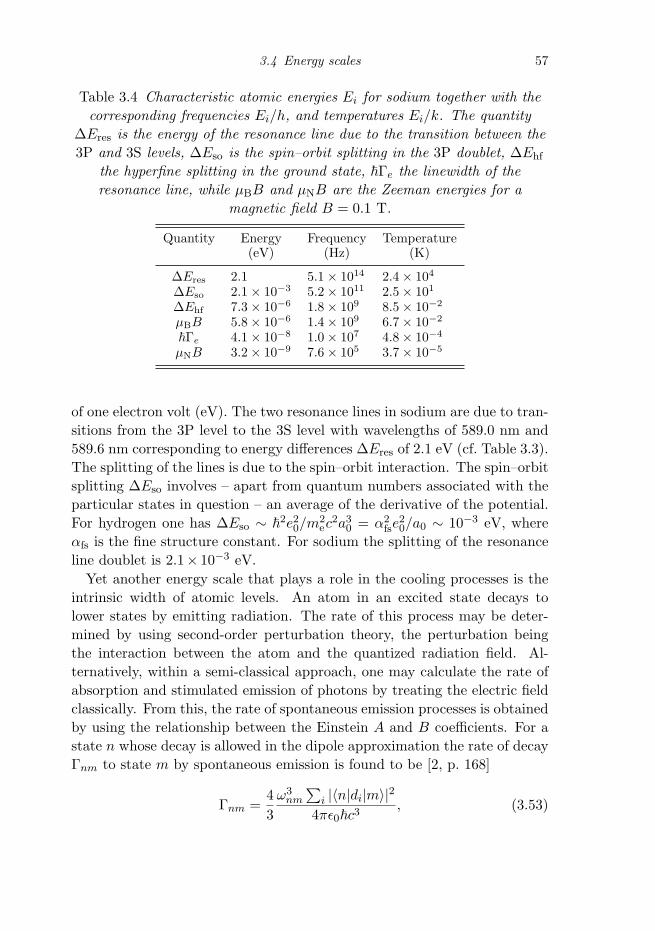
3.4 Energy scales 57
Table 3.4 Characteristic atomic energies Ei for sodium together with thecorresponding frequencies Ei/h, and temperatures Ei/k. The quantity
ΔEres is the energy of the resonance line due to the transition between the3P and 3S levels, ΔEso is the spin–orbit splitting in the 3P doublet, ΔEhf
the hyperfine splitting in the ground state, �Γe the linewidth of theresonance line, while μBB and μNB are the Zeeman energies for a
magnetic field B = 0.1 T.
Quantity Energy Frequency Temperature(eV) (Hz) (K)
ΔEres 2.1 5.1 × 10¹⁴ 2.4 × 10⁴
ΔEso 2.1 × 10⁻³ 5.2 × 10¹¹ 2.5 × 101
ΔEhf 7.3 × 10⁻⁶ 1.8 × 10⁹ 8.5 × 10⁻²
μBB 5.8 × 10⁻⁶ 1.4 × 10⁹ 6.7 × 10⁻²
�Γe 4.1 × 10⁻⁸ 1.0 × 10⁷ 4.8 × 10⁻⁴
μNB 3.2 × 10⁻⁹ 7.6 × 10⁵ 3.7 × 10⁻⁵
of one electron volt (eV). The two resonance lines in sodium are due to tran-sitions from the 3P level to the 3S level with wavelengths of 589.0 nm and589.6 nm corresponding to energy differences ΔEres of 2.1 eV (cf. Table 3.3).The splitting of the lines is due to the spin–orbit interaction. The spin–orbitsplitting ΔEso involves – apart from quantum numbers associated with theparticular states in question – an average of the derivative of the potential.For hydrogen one has ΔEso ∼ �
2e20/m2
ec2a3
0 = α2fse
20/a0 ∼ 10−3 eV, where
αfs is the fine structure constant. For sodium the splitting of the resonanceline doublet is 2.1× 10⁻³ eV.
Yet another energy scale that plays a role in the cooling processes is theintrinsic width of atomic levels. An atom in an excited state decays tolower states by emitting radiation. The rate of this process may be deter-mined by using second-order perturbation theory, the perturbation beingthe interaction between the atom and the quantized radiation field. Al-ternatively, within a semi-classical approach, one may calculate the rate ofabsorption and stimulated emission of photons by treating the electric fieldclassically. From this, the rate of spontaneous emission processes is obtainedby using the relationship between the Einstein A and B coefficients. For astate n whose decay is allowed in the dipole approximation the rate of decayΓnm to state m by spontaneous emission is found to be [2, p. 168]
Γnm =43
ω3nm
∑i |〈n|di|m〉|2
4πε0�c3, (3.53)

58 Atomic properties
where �ωnm is the energy difference between the levels in question, while〈n|di|m〉 is the dipole matrix element. This result is identical with thedamping rate of a classical electric dipole moment of magnitude equal tothe square root of
∑i |〈n|di|m〉|2 and oscillating with frequency ωnm. The
total decay rate of an excited state n is therefore given by
Γe =∑m
Γnm, (3.54)
where the sum is over all states m with energy less than that of the initialstate. Estimating (3.53) for the 2P–1S Lyman-α transition in hydrogen,with ωnm ∼ e2
0/�a0 and |〈n|di|m〉| ∼ ea0, yields
Γe ∼(
e20
�c
)3e20
�a0. (3.55)
The rate of spontaneous emission is thus a factor of order (αfs)3 or 4× 10⁻⁷
times atomic transition frequencies.For the resonance lines in alkali atoms, the possible final states are all
members of the ground-state multiplet, and therefore we may write thedecay rate (3.54) as
Γe ≈23fres
e20
�c
�ω2res
mec2, (3.56)
where ωres = ΔEres/� is the resonance-line frequency and fres is the totaloscillator strength from the excited state to all members of the ground-state multiplet. This strength, like the total strength from a member of theground-state multiplet to all members of the excited-state multiplet, is closeto unity, and for similar reasons, and therefore the decay rate of the excitedstate is given approximately by
Γe ≈23
e20
�c
�ω2res
mec2. (3.57)
For the resonance line in sodium, ωres ≈ 3.2 × 10¹⁵ s−1 and the estimate(3.57) gives Γe ≈ 6.4 × 10⁷ s−1, which agrees closely with the measuredvalue, 6.3 × 10⁷ s−1.
In Table 3.4 we list for sodium the characteristic energies, frequencies,and temperatures discussed above.
Problems
Problem 3.1 Calculate the Zeeman splitting of the hyperfine levels forthe 87Rb atom in low magnetic fields and determine the Lande g factors.

References 59
Problem 3.2 Use a high-field perturbation treatment to obtain explicitexpressions for the Zeeman-split hyperfine levels of 87Rb and 133Cs in astrong magnetic field and compare the results with Fig. 3.1.
Problem 3.3 The static polarizability of a hydrogen atom in its groundstate may be calculated in an approximate way from Eq. (3.34). First includeonly the unperturbed states |nlm〉 associated with the next-lowest unper-turbed energy level, which has n = 2, and show that if the electric fieldis in the z direction, the only non-vanishing matrix element is 〈210|z|100〉.Calculate the matrix element and use it to obtain a lower bound on themagnitude of the second-order correction to the energy, ΔE. Determine anupper bound on |ΔE| by replacing all the energy differences En −E0 in Eq.(3.34) by the difference between the energy of the lowest excited state andthat of the ground state, and use closure to evaluate the sum. The exactexpression, valid to second order in E , is ΔE/4πε0 = −(9/4)a3
0E2.
References[1] L. D. Landau and E. M. Lifshitz, Quantum Mechanics, Third edition,
(Oxford, Pergamon, 1977).[2] See, e.g., B. H. Bransden and C. J. Joachain, Physics of Atoms and
Molecules, (New York, Longman, 1983).[3] Experimental values of polarizabilities are taken from the compilation by
A. Derevianko, W. R. Johnson, M. S. Safronova, and J. F. Babb, Phys. Rev.Lett. 82, 3589 (1999).

4
Trapping and cooling of atoms
The advent of the laser opened the way to the development of powerfulmethods for producing and manipulating cold atomic gases. To set thestage we describe a typical experiment, which is shown schematically in Fig.4.1 [1]. A beam of sodium atoms emerges from an oven at a temperatureof about 600 K, corresponding to a speed of about 800 m s−1, and is thenpassed through a so-called Zeeman slower, in which the velocity of the atomsis reduced to about 30 m s−1, corresponding to a temperature of about 1 K.In the Zeeman slower, a laser beam propagates in the direction oppositethat of the atomic beam, and the radiation force produced by absorptionof photons retards the atoms. Due to the Doppler effect, the frequencyof the atomic transition in the laboratory frame is not generally constant,since the atomic velocity varies. However, by applying an inhomogeneousmagnetic field designed so that the Doppler and Zeeman effects cancel, thefrequency of the transition in the rest frame of the atom may be held fixed.On emerging from the Zeeman slower the atoms are slow enough to becaptured by a magneto-optical trap (MOT), where they are further cooledby interactions with laser light to temperatures of order 100 μK. Anotherway of compensating for the changing Doppler shift is to increase the laserfrequency in time, which is referred to as ‘chirping’. In other experimentsthe MOT is filled by transferring atoms from a second MOT where atomsare captured directly from the vapour. After a sufficiently large number ofatoms (typically 1010) have accumulated in the MOT, a magnetic trap isturned on and the laser beams are turned off: the atoms are then confinedby a purely magnetic trap. At this stage, the density of atoms is relativelylow, and the gas is still very non-degenerate, with a phase-space densityof order 10−6. The final step in achieving Bose–Einstein condensation isevaporative cooling, in which relatively energetic atoms leave the system,thereby lowering the average energy of the remaining atoms.
60

4.1 Magnetic traps 61
Fig. 4.1 A typical experiment to cool and trap alkali atoms.
In this chapter we describe the physics of cooling and trapping atoms.We begin with magnetic traps (Sec. 4.1). Subsequently, as a prelude to adiscussion of laser cooling and trapping, we consider the effects of laser ra-diation on atoms and describe optical traps (Sec. 4.2). We then discuss, inSec. 4.3, the theory of the Doppler process for laser cooling and, in Sec. 4.4,the magneto-optical trap. In Sec. 4.5 an account is given of the Sisyphuscooling process. Section 4.6 is devoted to evaporative cooling. Atomic hy-drogen is different from alkali atoms, in that it cannot be cooled by lasers,and the final section, Sec. 4.7, is devoted to experiments on hydrogen. Fora more extensive description of many of the topics treated in this chapter,see Ref. [2]. Other useful sources are the summer school lectures [3] and theNobel lectures [4, 5].
4.1 Magnetic traps
Magnetic trapping of neutral atoms is due to the Zeeman effect, which wedescribed in Chapter 3: the energy of an atomic state depends on the mag-netic field, and therefore an atom in an inhomogeneous field experiences aspatially varying potential. For simplicity, let us begin by assuming that theenergy of a state is linear in the magnetic field. As one can see from ourearlier discussion in Chapter 3 (see, e.g., Fig. 3.1), this is true generally forthe doubly polarized states, and for other states it is a good approximationprovided the level shifts produced by the magnetic field are either very smallor very large compared with the hyperfine splitting. The energy of an atomin a particular state i may then be written as
Ei = Ci − μiB, (4.1)

62 Trapping and cooling of atoms
where μi is the magnetic moment of the state and Ci is a constant. Themagnetic contribution to the energy thus provides a potential energy −μiB
for the atom. If the magnetic moment is positive, the atom experiences aforce tending to drive it to regions of higher field, while if it is negative,the force is towards regions of lower field. For this reason, states with apositive magnetic moment are referred to as high-field seekers, and thosewith a negative one as low-field seekers.
The energy depth of magnetic traps is determined by the Zeeman en-ergy, μiB. Atomic magnetic moments are of order the Bohr magneton,μB = e�/2me, which in temperature units is approximately 0.67 K/T. Sincelaboratory magnetic fields are generally considerably less than 1 tesla, thedepth of magnetic traps is much less than a kelvin, and therefore atomsmust be cooled in order to be trapped magnetically.
The task of constructing a magnetic trap is thus to design magnetic fieldconfigurations with either a local minimum in the magnitude of the magneticfield, or a local maximum. The latter possibility is ruled out by a generaltheorem that a local maximum in |B| is impossible in regions where thereare no electrical currents [6]. Thus the case of interest is that of a localminimum, and consequently the only atomic states that can be trapped bymagnetic fields alone are low-field seekers. Magnetic field configurationswith a local minimum in |B| have been important over the past few decadesfor trapping charged particles as a step in the continuing quest to realizenuclear fusion in hot plasmas. In this case the trapping results not fromthe intrinsic magnetic moment of the particle, but rather from the magneticmoment associated with its cyclotron motion. However, despite the verydifferent physical conditions in the two cases, the requirements in terms ofthe magnetic field configuration are quite similar, and the design of trapsfor cold atoms has been significantly influenced by work on plasmas. Fieldconfigurations with a minimum in |B| may be divided into two classes: oneswhere the minimum of the field is zero, and those where it is non-zero. Weshall now describe these in turn.
4.1.1 The quadrupole trap
A simple magnetic field configuration in which the magnetic field vanishesat some point is the standard quadrupole one, in which the magnetic fieldvaries linearly with distance in all directions. Such a magnetic field maybe produced by, e.g., a pair of opposed Helmholtz coils, as in standardfocusing magnets for controlling beams of charged particles in accelerators.For definiteness, let us consider a situation with axial symmetry about the

4.1 Magnetic traps 63
z direction. If we denote the magnetic field gradients along the x and y axesby B′, the gradient along the z axis must be −2B′, since the divergence ofthe magnetic field vanishes, ∇·B = 0. The magnetic field in the vicinity ofthe minimum, whose position we choose to be at the origin of the coordinatesystem, is thus given by
B = B′(x, y,−2z). (4.2)
The magnitude of the field is given by B = B′(x2 + y2 + 4z2)1/2, and thusit varies linearly with distance from the minimum, but with a slope thatdepends on direction.
The quadrupole trap suffers from one important disadvantage. In theabove discussion of the effective potential produced by a magnetic field, weassumed implicitly that atoms remain in the same quantum state. This isa good approximation provided the magnetic field experienced by an atomchanges slowly with time, since the atom then remains in the same quantumstate relative to the instantaneous direction of the magnetic field: it is said tofollow the magnetic field variations adiabatically. However, a moving atomexperiences a time-dependent magnetic field, which will induce transitionsbetween different states. In particular, atoms in low-field seeking states maymake transitions to high-field seeking ones, and thereby be ejected from thetrap. The effects of the time-dependent magnetic field become serious if itsfrequency is comparable with or greater than the frequencies of transitionsbetween magnetic sublevels. The latter are of order μBB, and thereforevanish if B = 0. Thus trap losses can be appreciable in the vicinity ofthe zero-field point: the quadrupole trap effectively has a ‘hole’ near thenode in the field, and this limits the time for which atoms can be storedin it.
This disadvantage of the simple quadrupole trap may be circumvented ina number of ways. One of these is to ‘plug the hole’ in the trap. In the firstsuccessful experiment to realize Bose–Einstein condensation this was doneby applying an oscillating bias magnetic field, as we shall explain in the nextsubsection. An alternative approach, adopted by the MIT group of Ketterleand collaborators in early experiments [7], is to apply a laser field in theregion of the node in the magnetic field. The resulting radiation forces repelatoms from the vicinity of the node, thereby reducing losses. The physics ofthis mechanism will be described in Sec. 4.2. Instead of using traps havinga node in the magnetic field, one can remove the ‘hole’ by working withmagnetic field configurations that have a non-zero field at the minimum.These will be described in Sec. 4.1.3.
64 Trapping and cooling of atoms
4.1.2 The TOP trap
As mentioned in Chapter 1, Bose–Einstein condensation in dilute gases wasfirst achieved in experiments using a modified quadrupole trap known as thetime-averaged orbiting potential (TOP) trap. In this trap one superimposeson the quadrupole field a rotating, spatially uniform, magnetic field [8]. Fordefiniteness we consider the geometry used in the original experiment, wherethe oscillating magnetic field has components B0 cos ωt in the x direction,and B0 sinωt in the y direction [9]. The instantaneous field is therefore givenby
B = (B′x + B0 cos ωt, B′y + B0 sinωt,−2B′z). (4.3)
Thus the effect of the oscillating bias field is to move the instantaneousposition of the node in the magnetic field. The frequency of the bias fieldis chosen to be low compared with the frequencies of transitions betweenmagnetic substates. This condition ensures that an atom will remain inthe same quantum state relative to the instantaneous magnetic field, andtherefore will not undergo transitions to other hyperfine states and be lostfrom the trap. Under these conditions the effect of the bias field may bedescribed in terms of an oscillatory component of the energy of an atom.If the frequency of the bias field is chosen to be much greater than that ofthe atomic motions, an atom moves in an effective potential given by thetime average of the instantaneous potential over one rotation period of thefield. In experiments, frequencies of atomic motions are typically ∼ 102 Hz,frequencies of transitions between magnetic substates are of order ∼ 106
Hz or more, and the frequency of the bias field is typically in the kilohertzrange.
To determine the effective potential we first evaluate the instantaneousstrength of the magnetic field, which is given by
B(t) = [(B0 cos ωt + B′x)2 + (B0 sin ωt + B′y)2 + 4B′2z2]1/2
� B0 + B′(x cos ωt + y sinωt)
+B′2
2B0[x2 + y2 + 4z2 − (x cos ωt + y sinωt)2], (4.4)
where the latter form applies for small distances from the node of the quadru-pole field, r |B0/B′|. The time average, <B>t, of the magnitude of themagnetic field over a rotation period of the field is defined by
<B>t =ω
2π
∫ 2π/ω
0dtB(t). (4.5)

4.1 Magnetic traps 65
By performing the time average, we find from (4.4) that
<B>t � B0 +B′2
4B0(x2 + y2 + 8z2). (4.6)
The important feature of this result is that the time-averaged field nevervanishes, and consequently there is no longer a ‘hole’ in the trap. Themagnetic contribution to the energy of an atom in a magnetic substate i isthus given for small r by
Ei(<B>t) � Ei(B0) − μi(B0)(<B>t − B0)
� Ei(B0) − μi(B0)B′2
4B0(x2 + y2 + 8z2), (4.7)
where
μi(B0) = −∂Ei
∂B
∣∣∣∣B0
(4.8)
is the projection of the magnetic moment in the direction of the magneticfield.1 The oscillating bias field thus converts the linear dependence of mag-netic field strength on distance from the node in the original quadrupolefield to a quadratic one, corresponding to an anisotropic harmonic-oscillatorpotential. The angular frequencies for motion in the three coordinate direc-tions are
ω2x = ω2
y = −μiB′2
2mB0, (4.9)
and
ω2z = 8ω2
x = −8μiB′2
2mB0. (4.10)
Different choices for the rotation axis of the bias field give traps with differentdegrees of anisotropy (see Problem 4.3).
Another force which can be important in practice is gravity. This givesrise to a potential which is linear in distance. If the potential produced bythe TOP trap were purely harmonic, the only effect of gravity would be todisplace the minimum in the harmonic-oscillator potential. However, theharmonic behaviour of the TOP trap potential extends only to a distanceof order l = B0/|B′| from the origin, beyond which the bias magnetic fieldhas little effect. If the gravitational force is strong enough to displace theminimum a distance greater than or of order B0/|B′|, the total potential no
1 For doubly polarized states, in which the nuclear and electron spins have the largest possibleprojections on the magnetic field direction and are in the same direction, the magnetic momentis independent of the magnetic field (see Sec. 3.2).

66 Trapping and cooling of atoms
longer has the form (4.7) when expanded about the new minimum. Gravitymodifies the trapping potential appreciably if the gravitational force mg,where g is the acceleration due to gravity, exceeds that due to the magnetictrap at a distance B0/|B′| from the origin. From Eq. (4.7) one sees thatthe force constant of the trap is of order |μi|B′2/B0, and therefore the forceat a distance B0/|B′| from the origin is of order |μiB
′|. Thus gravity isimportant if
|μiB′| � mg. (4.11)
By appropriate choice of magnetic field strengths and of the direction ofthe axis of a magnetic trap relative to that of the gravitational force it ispossible to make the minimum of the potential due to both magnetic andgravitational forces lie at a point such that the force constants of the trapare not in the usual ratio for a TOP trap in the absence of gravity.
4.1.3 Magnetic bottles and the Ioffe–Pritchard trap
An inhomogeneous magnetic field with a minimum in the magnetic field at anon-zero value may be generated by a configuration based on two Helmholtzcoils with identical currents circulating in the same direction, in contrast tothe simple quadrupole field, which is generated by Helmholtz coils with thecurrents in the two coils in opposite directions. Let us investigate the formof the magnetic field in the vicinity of the point midway between the coilson their symmetry axis, which we take to be the origin of our coordinatesystem. We denote the coordinate in the direction of the symmetry axisby z, and the distance from the axis by ρ. Since there are no currents inthe vicinity of the origin, the magnetic field may be derived from a scalarpotential Φ, B = −∇Φ. We assume the current coils to be rotationallysymmetric about the z axis, and thus the magnetic field is independent ofthe azimuthal angle. Since the field is an even function of the coordinates,the potential must be an odd one, and therefore an expansion of the potentialin terms of spherical harmonics Ylm can contain only terms with odd order l.Because of the rotational invariance about the symmetry axis, the potentialis a function only of the distance from the origin, r = (z2 + ρ2)1/2, andof cos θ = z/r. The potential satisfies Laplace’s equation, and it may bewritten simply as
Φ =∑
l
AlrlPl(z/r), (4.12)
where the Pl are Legendre polynomials and the Al are coefficients. Therecan be no terms with inverse powers of r since the field is finite at the origin.

4.1 Magnetic traps 67
In the immediate vicinity of the origin we may restrict ourselves to the firsttwo terms in this expansion, and therefore one has
Φ = A1rP1(cos θ) + A3r3P3(cos θ) (4.13)
= A1z + A3(52z3 − 3
2zr2) (4.14)
= A1z + A3(z3 − 32zρ2), (4.15)
and the magnetic field has components
Bz = −A1 − 3A3(z2 − 12ρ2), Bρ = 3A3zρ, and Bϕ = 0, (4.16)
where ϕ is the azimuthal angle. If A1 and A3 have the same sign, themagnetic field increases in magnitude with increasing |z|. Such a field con-figuration is referred to as a ‘magnetic bottle’ in plasma physics. Providedits energy is not too high, a charged particle gyrating about the field will bereflected as it moves towards regions of higher field, and thereby contained.Neutral particles, unlike charged ones, can move freely perpendicular to thedirection of the magnetic field, and therefore to trap them magnetically themagnetic field must increase in directions perpendicular to the magneticfield as well as parallel to it. To second order in z and ρ the magnitude ofthe magnetic field is given by
B = A1 + 3A3(z2 − 12ρ2), (4.17)
and therefore the magnetic field does not have a local minimum at the origin.The problem of creating a magnetic field with a local minimum in B arose
in the context of plasma physics, and one way of doing this was proposed byIoffe [10]. It is clear from the expansion of the potential given above that thiscannot be done if the magnetic field is axially symmetric: there are only twoadjustable coefficients, and there is no way to create a local minimum. Thesuggestion Ioffe made was to add to the currents creating the magnetic bottleother currents that break the rotational invariance about the symmetry axisof the bottle. In plasma physics the configuration used is that shown in Fig.4.2, where the additional currents are carried by conductors parallel to thesymmetry axis (so-called ‘Ioffe bars’). If the magnitude of the current is thesame for each bar, it follows from symmetry under rotation about the axisof the system that the potential produced by the currents in the bars mustcorrespond to a potential having components with degree m equal to 2 ormore. Thus the lowest-order spherical harmonics that can contribute areY2,±2 ∝ (ρ/r)2e±i2ϕ, and the corresponding solutions of Laplace’s equation
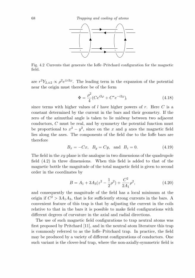
68 Trapping and cooling of atoms
Fig. 4.2 Currents that generate the Ioffe–Pritchard configuration for the magneticfield.
are r2Y2,±2 ∝ ρ2e±i2ϕ. The leading term in the expansion of the potentialnear the origin must therefore be of the form
Φ =ρ2
4(Cei2ϕ + C∗e−i2ϕ), (4.18)
since terms with higher values of l have higher powers of r. Here C is aconstant determined by the current in the bars and their geometry. If thezero of the azimuthal angle is taken to lie midway between two adjacentconductors, C must be real, and by symmetry the potential function mustbe proportional to x2 − y2, since on the x and y axes the magnetic fieldlies along the axes. The components of the field due to the Ioffe bars aretherefore
Bx = −Cx, By = Cy, and Bz = 0. (4.19)
The field in the xy plane is the analogue in two dimensions of the quadrupolefield (4.2) in three dimensions. When this field is added to that of themagnetic bottle the magnitude of the total magnetic field is given to secondorder in the coordinates by
B = A1 + 3A3(z2 − 12ρ2) +
C2
2A1ρ2, (4.20)
and consequently the magnitude of the field has a local minimum at theorigin if C2 > 3A1A3, that is for sufficiently strong currents in the bars. Aconvenient feature of this trap is that by adjusting the current in the coilsrelative to that in the bars it is possible to make field configurations withdifferent degrees of curvature in the axial and radial directions.
The use of such magnetic field configurations to trap neutral atoms wasfirst proposed by Pritchard [11], and in the neutral atom literature this trapis commonly referred to as the Ioffe–Pritchard trap. In practice, the fieldmay be produced by a variety of different configurations of conductors. Onesuch variant is the clover-leaf trap, where the non-axially-symmetric field is

4.1 Magnetic traps 69
Fig. 4.3 Schematic view of the currents in the clover-leaf trap.
produced by coils configured as shown in Fig. 4.3 [1]. The windings lookvery different from the Ioffe bars, but since the azimuthal symmetry of thecurrents corresponds to m = 2 or more, as in the Ioffe case, the field near theorigin must have the same symmetry. To first order in the coordinates thecomponent of the magnetic field in the axial direction vanishes, and the firstnon-vanishing contributions are of third order. A virtue of the clover-leafconfiguration relative to the original Ioffe one is that experimental accessto the region near the field minimum is easier due to the absence of thecurrent-carrying bars.
4.1.4 Microtraps
Cold atoms can be manipulated and transported by using traps in the form ofmicro-fabricated current-carrying conductors. As a simple example, consideran infinitely long, straight wire along the z axis carrying a current I, withan external magnetic field, which we refer to as the bias field, of strength B0
applied perpendicular to the wire in the x direction, as shown in Fig. 4.4 (a).According to Ampere’s law, the magnitude of the magnetic field BI due tothe current in the wire is given by BI = μ0I/2πρ, where ρ is the distancefrom the wire.
The magnetic field produced by the current in the wire is in the azimuthaldirection with respect to the wire, and therefore the superposition of this

70 Trapping and cooling of atoms
z
I
y
B0
x
z
z
x
(a)
(c)
(b)
y=y0/2
Fig. 4.4 (a) The two-dimensional microtrap. (b) Contours of constant B. (c) The‘U’ and ‘Z’ configurations.
field and the bias field vanishes on a line parallel to the conductor and inthe plane x = 0. This therefore creates a trapping potential in the xy planefor atoms in low-field seeking states. The total magnetic field on the line(x, y) = ρ(cos φ, sinφ) is thus given by
Bx = B0 − BI sinφ, By = BI cos φ, (4.21)
and its magnitude is B = (B2I + B2
0 − 2BIB0 sinφ)1/2. This vanishes whenφ = π/2 and BI(ρ) = B0, corresponding to x = 0 and y = y0 = Iμ0/2πB0.The contours of constant B in the xy plane are circles and the line y = y0/2(on which B = B0), as illustrated in Fig. 4.4 (b).
The trap is two-dimensional, but it can be closed in the z direction bybending the wire in the x direction into the forms shown in Fig. 4.4 (c), whichare referred to as ‘U’ and ‘Z’ configurations, respectively. The currents inthe parts of the wire parallel to the x axis produce a magnetic field inthe z direction, and this cannot be compensated by the bias field. As aconsequence, the magnitude of the minimum value of the total magnetic

4.2 Influence of laser light on an atom 71
field in the plane perpendicular to the z axis increases as |z| increases fromzero.
By superimposing two such configurations of conductors it is possible tomake a trap with a minimum whose position depends on the currents in thetwo conductors. With a series of such configurations a succession of fieldmaxima and minima may be created [12], and by applying currents whosemagnitudes vary in time, it is possible to shift the positions of the minima,thereby producing a ‘conveyor belt’ which can transport over macroscopicdistances atoms trapped near the minima [13]. For a review of microtraps,see Ref. [14].
4.2 Influence of laser light on an atom
Many techniques for trapping and cooling atoms exploit the interaction ofatoms with radiation fields, especially those of lasers. As a prelude to theapplications later in this chapter, we give here a general description of theinteraction of an atom with a radiation field. In Sec. 3.3 we calculated thepolarizability of atoms with non-degenerate ground states, and here we shallgeneralize the treatment to allow for the lifetime of the excited state, andarbitrary directions for the electric field.
The interaction between an atom and the electric field is given in thedipole approximation by
H ′ = −d·E, (4.22)
where d is the electric dipole moment operator and E is the electric fieldvector. In a static electric field the change ΔEg in the ground-state energyof an atom is given to second order in the electric field by
ΔEg = −∑
e
|〈e|H ′|g〉|2Ee − Eg
= −12αE2, (4.23)
where
α = 2∑
e
|〈e|d·ε|g〉|2Ee − Eg
(4.24)
is the atomic polarizability. Here ε is a unit vector in the direction of theelectric field, and we label the ground state by g and the excited statesby e. This contribution to the energy may be represented by the diagramshown in Fig. 4.5 (a). The interaction vertices give factors 〈e|(−d·E)|g〉 and〈g|(−d·E)|e〉, and the line for the intermediate atomic state gives a factor1/(Ee − Eg) to the summand, as one may confirm by comparing with theexplicit calculation in Sec. 3.3.
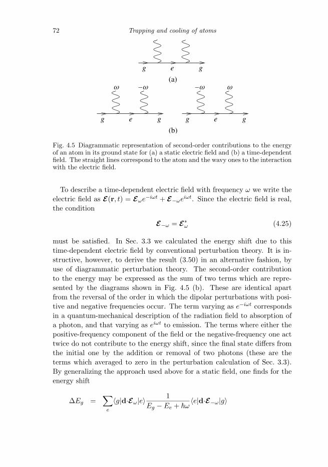
72 Trapping and cooling of atoms
Fig. 4.5 Diagrammatic representation of second-order contributions to the energyof an atom in its ground state for (a) a static electric field and (b) a time-dependentfield. The straight lines correspond to the atom and the wavy ones to the interactionwith the electric field.
To describe a time-dependent electric field with frequency ω we write theelectric field as E(r, t) = Eωe−iωt + E−ωeiωt. Since the electric field is real,the condition
E−ω = E∗ω (4.25)
must be satisfied. In Sec. 3.3 we calculated the energy shift due to thistime-dependent electric field by conventional perturbation theory. It is in-structive, however, to derive the result (3.50) in an alternative fashion, byuse of diagrammatic perturbation theory. The second-order contributionto the energy may be expressed as the sum of two terms which are repre-sented by the diagrams shown in Fig. 4.5 (b). These are identical apartfrom the reversal of the order in which the dipolar perturbations with posi-tive and negative frequencies occur. The term varying as e−iωt correspondsin a quantum-mechanical description of the radiation field to absorption ofa photon, and that varying as eiωt to emission. The terms where either thepositive-frequency component of the field or the negative-frequency one acttwice do not contribute to the energy shift, since the final state differs fromthe initial one by the addition or removal of two photons (these are theterms which averaged to zero in the perturbation calculation of Sec. 3.3).By generalizing the approach used above for a static field, one finds for theenergy shift
ΔEg =∑
e
〈g|d·Eω|e〉1
Eg − Ee + �ω〈e|d·E−ω|g〉

4.2 Influence of laser light on an atom 73
+∑
e
〈g|d·E−ω|e〉1
Eg − Ee − �ω〈e|d·Eω|g〉
=∑
e
|〈e|d·ε|g〉|2(
1Eg − Ee − �ω
+1
Eg − Ee + �ω
)|Eω|2
= −α(ω)|Eω|2
= −12α(ω)<E(r, t)2>t, (4.26)
where < · · ·>t denotes a time average, and the dynamical polarizability isgiven by
α(ω) =∑
e
|〈e|d·ε|g〉|2(
1Ee − Eg + �ω
+1
Ee − Eg − �ω
)
=∑
e
2(Ee − Eg)|〈e|d·ε|g〉|2
(Ee − Eg)2 − (�ω)2, (4.27)
in agreement with Eqs. (3.50) and (3.51). Note that the only difference fromthe static case is that the intermediate energy denominators are shifted by±�ω to take into account the non-zero frequency of the electric field.
In many situations of interest the frequency of the radiation is close tothat of an atomic resonance, and it is then a good approximation to ne-glect all transitions except the resonant one. In addition, in the expressionfor the polarizability one may take only the term with the smallest energydenominator. The polarizability then reduces to a single term
α(ω) ≈ |〈e|d·ε|g〉|2Ee − Eg − �ω
. (4.28)
In the above discussion we implicitly assumed that the excited state hasan infinitely long lifetime. However, in reality it will decay by spontaneousemission of photons. This effect can be taken into account phenomenologi-cally by attributing to the excited state an energy with both real and imag-inary parts. If the excited state has a lifetime 1/Γe, corresponding to thee-folding time for the occupation probability of the state, the correspondinge-folding time for the amplitude will be twice this, since the probability isequal to the squared modulus of the amplitude. If, in the usual way, theamplitude of the excited state is taken to vary as exp(−iEet/�), exponentialdecay of the amplitude with a lifetime 2/Γe corresponds to an imaginarycontribution to the energy of the state equal to −i�Γe/2. The polarizabilityis then
α(ω) ≈ |〈e|d·ε|g〉|2Ee − i�Γe/2 − Eg − �ω
. (4.29)

74 Trapping and cooling of atoms
Quite generally, the energy of the ground state is a complex quantity, andwe shall write the energy shift as
ΔEg = Vg − i�Γg/2. (4.30)
This has the form of an effective potential acting on the atom, the real partcorresponding to a shift of the energy of the state, and the imaginary partto a finite lifetime of the ground state due to transitions to the excited stateinduced by the radiation field, as described above. The shift of the energylevel is given by
Vg = −12α′(ω)<E(r, t)2>t, (4.31)
where
α′(ω) ≈ (Ee − Eg − �ω)|〈e|d·ε|g〉|2(Ee − Eg − �ω)2 + (�Γe/2)2
(4.32)
is the real part of α. These shifts are sometimes referred to as ac Starkshifts, since the physics is the same as for the usual Stark effect except thatthe electric field is time-dependent.
It is convenient to introduce the detuning, δ, which is the difference be-tween the laser frequency and the frequency ωeg = (Ee−Eg)/� of the atomictransition:
δ = ω − ωeg. (4.33)
Positive δ is referred to as blue detuning, and negative δ as red detuning.The energy shift is given by
Vg =�Ω2
Rδ
δ2 + Γ2e/4
. (4.34)
Here we have introduced the Rabi frequency, which is the magnitude of theperturbing matrix element |〈e|d·Eω|g〉| expressed as a frequency:
ΩR = |〈e|d·Eω|g〉|/�. (4.35)
Ground-state energy shifts are thus positive for blue detuning and negativefor red detuning.
The rate of loss of atoms from the ground state is given by
Γg = −2�
Im ΔEg =1�α′′(ω)<E(r, t)2>t, (4.36)
where α′′ is the imaginary part of α,
α′′(ω) ≈ �Γe/2(Ee − Eg − �ω)2 + (�Γe/2)2
|〈e|d·ε|g〉|2. (4.37)

4.2 Influence of laser light on an atom 75
Thus the rate of transitions from the ground state has a Lorentzian de-pendence on frequency in this approximation. In the limit Γe → 0, theLorentzian becomes a Dirac delta function and Eq. (4.36) is then equivalentto Fermi’s Golden Rule for the transition rate.
The perturbative treatment given above is valid provided the admixtureof the excited state into the ground state is small. To lowest order in theperturbation, this admixture is of order the matrix element of the perturba-tion divided by the excitation energy of the intermediate state. If the decayof the intermediate state may be neglected, the magnitude of the energy de-nominator is |�(ωeg − ω)| = �|δ| and, with allowance for decay, the effectiveenergy denominator has a magnitude �(δ2 + Γ2
e/4)1/2. The condition forvalidity of perturbation theory is therefore |〈e|d·Eω|g〉| �(δ2 + Γ2
e/4)1/2
or ΩR (δ2 + Γ2e/4)1/2. For larger electric fields it is necessary to go be-
yond simple perturbation theory but, fortunately, under most conditionsrelevant for experiments on Bose–Einstein condensation, electric fields areweak enough that the perturbative approach is adequate.
4.2.1 Forces on an atom in a laser field
Experiments on clouds of dilute gases exploit the forces on atoms in a laserfield in a variety of ways. Before discussing specific applications, we describethe origin of these forces. The energy shift of an atom may be regarded asan effective potential V in which the atom moves. This way of viewingthe problem is sometimes referred to as the dressed atom picture, since theenergy of interest is that of an atom with its accompanying perturbationsin the radiation field, not just an isolated atom. It is the analogue of theconcept of an elementary excitation, or quasiparticle, that has been so pow-erful in understanding the properties of solids and quantum liquids. If thetime-averaged electric field varies with position, the shift of the energy dueto the field gives rise to a force
Fdipole = −∇V (r) =12α′(ω)∇ <E(r, t)2>t (4.38)
on an atom. Here < · · · >t denotes a time average. This result may beunderstood as being due to the interaction of the induced dipole momentof the atom with a spatially varying electric field, and it is often referredto as the dipole force. More generally, terms due to higher moments of theelectric charge distribution such as the quadrupole moment will also giverise to forces, but these will usually be much less than the dipole force.
At low frequencies the polarizability is positive, and the dipole moment

76 Trapping and cooling of atoms
is in the same direction as the electric field. However, at frequencies abovethose of transitions contributing importantly to the polarizability, the in-duced dipole moment is in the opposite direction, as one can see by in-spection of Eq. (4.32). It is illuminating to consider a frequency close to aresonance, in which case we may use the approximate form (4.32) for the realpart of the polarizability. From this one can see that for frequencies belowthe resonance the force is towards regions of higher electric field, while forones above it the force is towards regions of lower field. As can be seen fromEqs. (4.38) and (4.32), the magnitude of the force can be of order ωeg/Γe
times larger than for static fields of the same strength.As we remarked above, the radiation force repelling atoms from regions
of high electric field at frequencies above resonance has been used to reduceloss of atoms at the centre of a quadrupole trap [7]. A blue-detuned laserbeam passing through the trap centre gave a repulsive contribution to theenergy of atoms, which were thereby prevented from penetrating into thedangerous low-field region, where spin flips could occur.
The change in sign of the force at resonance may be understood in termsof a classical picture of an electron moving in a harmonic potential under theinfluence of an electric field. The equation of motion for the atomic dipolemoment d = −er, where r is the coordinate of the electron, is
d2ddt2
+ ω20d =
e2
meE, (4.39)
with ω0 being the frequency of the harmonic motion. For an electric fieldwhich oscillates in time as exp(−iωt), we then obtain
(−ω2 + ω20)d =
e2
meE. (4.40)
This shows that the polarizability, the ratio of the dipole moment to theelectric field, is
α(ω) =e2
me(ω20 − ω2)
, (4.41)
which becomes negative for frequencies ω that exceed ω0. If we comparethis result with the quantum-mechanical one, Eq. (3.52), we see that itcorresponds to having oscillator strength unity for a single transition at theoscillator frequency.
In addition to the contribution to the force on an atom due to energy-levelshifts, which are associated with virtual transitions between atomic states,there is another one due to real transitions. Classically this is due to theradiation pressure on the atom. In quantum-mechanical language it is a
4.2 Influence of laser light on an atom 77
consequence of the momentum of a photon being imparted to or removedfrom an atom during an absorption or an emission process. The rate ofabsorption of photons by an atom in the ground state is equal to the rate ofexcitation of the ground state, given by (4.36). Therefore, if the radiationfield is a travelling wave with wave vector q, the total force on the atom dueto absorption processes is
Frad = �qΓg. (4.42)
As we shall describe, both this force and the dipole force (4.38) play animportant role in laser cooling.
4.2.2 Optical traps
A focused laser beam creates a radiation field whose intensity has a maxi-mum in space. If the frequency of the light is detuned to the red, the energyof a ground-state atom has a spatial minimum, and therefore it is possibleto trap atoms. The depth of the trap is determined by the magnitude of theenergy shift, given by Eq. (4.34).
One advantage of optical traps is that the potential experienced by analkali atom in its ground state is essentially independent of the magneticsubstate. This is due to the fact that the ground state of alkali atoms is anS state (see Sec. 3.3). The situation is quite different for trapping by mag-netic fields, since the potential is then strongly dependent on the magneticsubstate. With magnetic traps it is difficult to investigate the influence ofthe interaction energy on the spin degrees of freedom of an atomic cloudsince the energy is dominated by the Zeeman term. By contrast, opticaltraps are well suited for this purpose.
Optical traps are also important in the context of Feshbach resonances.As we shall describe in Sec. 5.4.2, in the vicinity of such a resonance theeffective interaction is a strong function of the magnetic field, and thereforeit is desirable that the magnetic field be homogeneous. This may be achievedby applying a uniform magnetic field to atoms in an optical trap, but it is notpossible with magnetic traps, since without inhomogeneity of the magneticfield there is no trapping.
To reduce heating of atoms by absorption of photons, the laser frequencyin optical traps must be chosen to be away from atomic resonances. In anearly experiment, a Bose–Einstein condensate of Na atoms was held in apurely optical trap by Stamper-Kurn et al. [15]. The laser had a wavelengthof 985 nm while that of the atomic transition is 589 nm. The resulting opticaltraps are shallow, with depths of order μK in temperature units (see Prob-

78 Trapping and cooling of atoms
lem 4.4), and therefore atoms are usually precooled in other sorts of trapsbefore they can be held by purely optical forces. However, a Bose–Einsteincondensate of 87Rb atoms has been created in an optical trap formed by twocrossed laser beams, without the need for magnetic traps [16]. Evaporativecooling of the gas, which was a mixture of atoms in the three hyperfine statesF = 1 and mF = 0,±1, was achieved by gradually lowering the power in thelaser beams, thus reducing the depth of the trap. The resulting condensatecontained 3.5 × 10⁴ atoms. Further reduction of the laser power resulted inrapid loss of atoms, since the trap was then so shallow that it was unable tosupport the cloud against gravity.
4.3 Laser cooling: the Doppler process
The basic idea that led to the development of laser cooling may be under-stood by considering an atom subjected to two counter-propagating laserbeams of the same angular frequency, ω, and the same intensity. Imaginethat the frequency of the laser beams is tuned to lie just below the frequency,ωeg, of an atomic transition between an excited state |e〉 and the ground state|g〉. For definiteness we assume that the laser beams are directed along thez axis.
To estimate the frictional force, we assume that the radiation field issufficiently weak that the absorption may be calculated by perturbationtheory. From Eqs. (4.36) and (4.37), the rate dNph/dt at which a singleatom absorbs photons from one of the beams is given by
dNph
dt= CL(ω), (4.43)
where
C =π
�2|〈e|d·ε|g〉|2 <E(r, t)2>t (4.44)
and L is the Lorentzian function
L(ω) =Γe/2π
(ω − ωeg)2 + (Γe/2)2, (4.45)
which is normalized so that its integral over ω is unity. The lifetime ofan atom in the ground state in the presence of one of the laser beams is1/CL(ω). An atom initially at rest will absorb as many left-moving photonsas right-moving ones, and thus the total momentum change will be zeroon average. However, for an atom moving to the right with velocity vz,the frequency of the right-moving photons in the rest frame of the atomis decreased due to the Doppler effect, and to lowest order in the velocity

4.3 Laser cooling: the Doppler process 79
Fig. 4.6 Rate of absorption of photons from the two red-detuned laser beams asfunctions of the atomic velocity.
it is given by ω − vzq, where q = ω/c is the wave number of the photons.The frequency thus lies further from the atomic resonance than it would foran atom at rest, and consequently the rate of absorption of right-movingphotons is reduced, and is given approximately by
dNright
dt= CL(ω − vzq). (4.46)
For photons moving to the left the story is the opposite: the frequencyof the photons in the rest frame of the atom is increased to ω + vzq, andconsequently absorption of these photons is increased:
dNleft
dt= CL(ω + vzq). (4.47)
The situation is represented schematically in Fig. 4.6, where we show theabsorption of photons from the two beams as functions of the velocity of theatom.
Since in absorbing a photon, the atom receives momentum �q in the di-rection of propagation of the photon, the absorption of photons from thetwo laser beams produces a frictional force on the atom. The net rate oftransfer of momentum to the atom is given by
dpz
dt= −γvz, (4.48)
where the friction coefficient γ is defined by
γ =�qC
vz[L(ω + vzq) − L(ω − vzq)] � 2�q2C
dL(ω)dω
. (4.49)
In the second expression in Eq. (4.49) we have assumed that the atom movessufficiently slowly that the Doppler shift is small compared with the larger

80 Trapping and cooling of atoms
of the linewidth and the detuning. The characteristic braking time, whichdetermines the rate of loss of momentum by an atom, is given by
1τfric
= − 1pz
dpz
dt=
γ
m. (4.50)
For narrow lines, dL/dω can be very large in magnitude if the detuning is oforder Γe and in that case the frictional force is correspondingly large. Be-cause of this, the configuration of oppositely directed laser beams is referredto as optical molasses. The frictional force is strong only for a limited rangeof velocities because, if the velocity of the atom exceeds the larger of Γe/q
and |δ|/q, the linear expansion fails, and the force is reduced.We now estimate the lowest atomic kinetic energies that one would ex-
pect to be attainable with the configuration described above. Absorptionof photons by atoms, as well as giving rise to the frictional force, also heatsthem. An atom at rest is equally likely to absorb photons from either ofthe beams and, since absorption events are uncorrelated with each other,the momentum of the atom undergoes a random walk. In such a walk, themean-square change in a quantity is the total number of steps in the walktimes the square of the step size. The total number of photons absorbed perunit time is given by
dNph
dt= 2CL(ω), (4.51)
since for small velocities the Doppler shifts may be neglected, and thereforethe momentum diffusion coefficient, which is the rate of change of the mean-square momentum p2
z of the atom due to absorption of photons, is given by
dp2z
dt
∣∣∣∣∣abs
= 2CL(ω)(�q)2. (4.52)
The emission of photons as the atom de-excites also contributes to the ran-dom walk of the momentum. Just how large this effect is depends on detailedassumptions about the emission pattern. If one makes the somewhat arti-ficial assumption that the problem is purely one-dimensional, and that thephotons are always emitted in the direction of the laser beams, the step sizeof the random walk for the z momentum of the atom is again �q, and thetotal number of photons emitted is equal to the number absorbed. Thus therate of change of the mean-square momentum is precisely the same as forabsorption,
dp2z
dt
∣∣∣∣∣em
=dp2
z
dt
∣∣∣∣∣abs
. (4.53)

4.3 Laser cooling: the Doppler process 81
The total momentum diffusion coefficient, Dp, due to both absorption andemission of photons is thus given by
Dp =dp2
z
dt
∣∣∣∣∣heat
= 4CL(ω)(�q)2. (4.54)
The kinetic energy of the atom in a steady state is determined by balancingthe heating rate (4.54) with the cooling due to the frictional force which,from (4.48) and (4.50), is given by
dp2z
dt
∣∣∣∣∣fric
= −2p2
z
τfric. (4.55)
One thus arrives at the equation
p2z =
12Dpτfric, (4.56)
which shows that the root-mean-square momentum in a steady state is,roughly speaking, the momentum an atom would acquire during a randomwalk of duration equal to the braking time τfric of an atom in the groundstate. Thus the mean kinetic energy and temperature T associated with themotion of the atom in the z direction are given by
mv2z = kT = �L(ω)
(dL(ω)
dω
)−1
. (4.57)
The lowest temperature attainable by this mechanism is obtained by mini-mizing this expression with respect to ω, and is found from (4.45) to be
kT =�Γe
2. (4.58)
For other assumptions about the emission of photons from the excited state,the limiting temperature differs from this result by a numerical factor. Interms of the detuning parameter δ = ω − ωeg, the minimum temperature isattained for δ = −Γe/2, corresponding to red detuning. For blue detuning,the atom is accelerated rather than slowed down, as one can see from thegeneral formula for the force.
As an example, let us estimate the lowest temperature that can beachieved by laser cooling of sodium atoms. Since the width Γe correspondsto a temperature of 480 μK according to Table 3.4, we conclude that theminimum temperature attainable by the Doppler mechanism is ≈ 240 μK.In our discussion above we have shown how cooling is achieved for one veloc-ity component. With three pairs of mutually opposed laser beams all threecomponents of the velocity may be cooled.

82 Trapping and cooling of atoms
As we mentioned in the introduction to this chapter, in some experimentsatoms are passed through a so-called Zeeman slower to reduce their velocitiesto values small enough for trapping in a magneto-optical trap to be possible.In the Zeeman slower a beam of atoms is subjected to a single laser beampropagating in the direction opposite that of the atoms. As we have seenearlier in this section, absorption and subsequent re-emission of radiationby atoms transfers momentum from the laser beam to the atoms, therebyslowing the atoms. However, if the frequency of the laser beam is resonantwith the atomic frequency when atoms emerge from the oven, the slowingof the atoms and the consequent change of the Doppler shift will causethe transition to become non-resonant. Thus the velocity range over whichlaser light will be maximally effective in decelerating atoms is limited. In theZeeman slower the effect of the decreasing atomic velocity on the frequencyof the atomic transition is compensated by a Zeeman shift produced by aninhomogeneous magnetic field.
4.4 The magneto-optical trap
Radiation pressure may also be used to confine atoms in space. In themagneto-optical trap (MOT) this is done with a combination of laser beamsand a spatially varying magnetic field. The basic physical effect is that,because atomic energy levels depend on the magnetic field, the radiationpressure depends on position. By way of illustration, consider an atom witha ground state having zero total angular momentum, and an excited statewith angular momentum quantum number J = 1. For simplicity we neglectthe nuclear spin. Consider, for example, the quadrupole magnetic field (4.2).On the z axis, the magnetic field is in the z direction and it is linear in z.The magnetic substates of the excited state are specified by the quantumnumber m, in terms of which the projection of the angular momentum ofthe state along the z axis is m�. Circularly polarized laser beams with equalintensity and frequency are imposed in the positive and negative z directions.The polarization of both beams is taken to be clockwise with respect to thedirection of propagation, which means that the beam directed to the right(σ+) couples the ground state to the m = +1 excited substate. On the otherhand, the polarization of the beam directed to the left has the opposite sense(σ−) with respect to the z axis, and thus induces transitions to the m = −1substate. The situation is shown schematically in Fig. 4.7.
Let us assume that the laser frequency is detuned to the red. At z = 0the two laser beams are absorbed equally by the atom, and thus there isno net radiation force on the atom. However, if the atom is displaced to

4.4 The magneto-optical trap 83
Fig. 4.7 (a) The magneto-optical trap. (b) The relevant transitions. (c) Influenceof a spatially varying magnetic field on the atomic transitions. (After Ref. [16].)
positive values of z, the frequency of the transition to the m = −1 substateis reduced, and is thus closer to the laser frequency, while the reverse holdsfor the m = +1 substate. This results in an increased absorption rate for σ−photons, which are moving to the left, and a decreased rate for σ+ photons,which are moving to the right. Consequently there is a force towards the ori-gin, where the two transitions have the same frequency. Similar argumentsapply for negative z. Determining the force constant for the trap is thetask of Problem 4.5. By applying six laser beams, two counter-propagatingbeams along each axis, one can make a three-dimensional trap.
The use of MOTs is an almost universal feature of experiments on coldatoms. Not only do they trap atoms, but they also cool them, since theDoppler mechanism described above and the Sisyphus process describedbelow operate in them. The fact that the atomic frequency depends onposition, due to the inhomogeneous magnetic field, implies that efficientcooling is possible for atoms with a range of velocities.
In practice, MOTs are more complicated than the simple schematic modeldescribed above. One reason for this is that the ground state of an alkali

84 Trapping and cooling of atoms
atom has more than one hyperfine state. As an example let us considerNa, which has F = 2 and F = 1 hyperfine levels of the 3S1/2 ground state.The excited 3P3/2 state has hyperfine levels with total angular momentumquantum numbers F ′ = 0, 1, 2, and 3. If laser light resonant with theF = 2 → F ′ = 3 transition is applied, some atoms will be excited non-resonantly to the F ′ = 2 state, from which they will decay either to theF = 2 or F = 1 levels of the ground state. Since there is no radiationresonant with the F = 1 → F ′ = 2 transition, the net effect is to buildup the population of atoms in the F = 1 level compared with that in theF = 2 level. This process is referred to as optical pumping. If this depletionof atoms in the F = 2 level is not hindered, the MOT will cease to workeffectively because of the small number of atoms in the F = 2 level, referredto as the bright state, which is the one involved in the transition the MOT isworking on. To remove atoms from the F = 1 level, radiation resonant withthe F = 1 → F ′ = 2 transition is applied. This is referred to as repumping.
As we shall explain below, for evaporative cooling to be effective it is nec-essary to achieve a sufficiently high density of atoms. In a standard MOTthere are a number of effects which limit the density to values too low forevaporative cooling to be initiated. One of these is that the escaping fluo-rescent radiation produces a force on atoms which counteracts the trappingforce of the MOT. A second is that if the density is sufficiently high, thecloud becomes opaque to the trapping light. Both of these can be mitigatedby reducing the amount of repumping light so that only a small fractionof atoms are in the substate relevant for the transition on which the MOToperates. This reduces the effective force constant of the MOT, but thedensity that can be attained with a given number of atoms increases. In theexperiment of Ketterle et al. [18] repumping light was applied preferentiallyin the outer parts of the cloud, thereby giving rise to strong frictional forceson atoms arriving from outside, while in the interior of the cloud radiationforces were reduced because of the depletion of atoms in the bright state.Such a trap is referred to as a dark-spot MOT, and densities achievable withit are of order 100 times higher than with a conventional MOT. The dark-spot MOT made it possible to create clouds with densities high enough forevaporative cooling to be efficient, and it was a crucial element in the earlyexperiments on Bose–Einstein condensation in alkali atom vapours.
4.5 Sisyphus cooling
It was encouraging that the temperatures achieved in early experiments onlaser cooling appeared to agree with the estimates made for the Doppler

4.5 Sisyphus cooling 85
mechanism. However, subsequent studies showed that temperatures belowthe Doppler value could be realized, and that this happened for large de-tunings, not for a detuning equal to Γe/2 as the Doppler theory predicts.This was both gratifying, since it is commonly the case that what can beachieved in practice falls short of theoretical prediction, and disquieting,since the measurements demonstrated that the cooling mechanisms werenot understood [19]. In addition, experimental results depended on the po-larization of the laser beams. This led to the discovery of new mechanismswhich can cool atoms to temperatures corresponding to a thermal energy oforder the so-called recoil energy,
Er =(�q)2
2m. (4.59)
This is the kinetic energy imparted to an atom at rest when it absorbs aphoton of momentum �q, and it corresponds to a temperature
Tr =Er
k=
(�q)2
2mk. (4.60)
These temperatures lie several orders of magnitude below the lowest tem-perature achievable by the Doppler mechanism, since the recoil energy is�
2ω2/2mc2. The atomic transitions have energies on the scale of elec-tron volts, while the rest-mass energy of an atom is ≈ A GeV, whereA is the mass number of the atom. The recoil energy is thereforeroughly 5 × 10⁻¹⁰(�ω/1eV)2/A eV, and the corresponding temperature is≈ 6 × 10⁻⁶(�ω/1eV)2/A K, which is of order 0.1–1 μK.
The new cooling mechanisms rely on two features not taken into accountin the Doppler theory. First, alkali atoms are not simple two-level systems,and their ground states have substates which are degenerate in the absenceof a magnetic field, as we saw in Chapter 3. Second, the radiation fieldproduced by two opposed laser beams is inhomogeneous. To understandhow one of these mechanisms, the so-called Sisyphus process, works, considertwo counter-propagating, linearly polarized laser beams of equal intensity.For definiteness, we assume that the beam propagating in the positive z
direction is polarized along the x axis, while the one propagating in thenegative z direction is polarized in the y direction. The electric field is thusof the form
E(z, t) = E(z)e−iωt + E∗(z)eiωt, (4.61)
where
E(z) = E0(exeiqz + eye−iqz). (4.62)

86 Trapping and cooling of atoms
32
12
12
32
13
32
32
gg
11
Fig. 4.8 Dipole transitions between a doublet ground state and a quadruplet excitedstate. The numbers indicate the square of the Clebsch–Gordan coefficients for thetransitions.
In writing this equation we have chosen the origin of the coordinate sys-tem to eliminate the arbitrary phase difference between the two counter-propagating beams. Thus the polarization of the radiation field varies withz, and the normalized polarization vector is
ε =1√2(exeiqz + eye
−iqz) =1√2eiqz(ex + eye
−2iqz). (4.63)
Apart from an overall phase factor, this varies regularly in the z directionwith a period π/q, which is one-half of the optical wavelength, λ = 2π/q.At z = 0 the electric field is linearly polarized at 45◦ to the x axis, andat z = λ/4 it is again linearly polarized, but at an angle −45◦ to the x
axis. At z = λ/8 the electric field is circularly polarized with negative sense(σ−) about the z axis, while at z = 3λ/8 it is circularly polarized withpositive sense (σ+). At an arbitrary point the intensities of the positivelyand negatively circularly polarized components of the radiation field varyas (1 ∓ sin 2qz)/2, as may be seen by expressing (4.62) in terms of thepolarization vectors (ex ± iey)/
√2.
The periodic potential
As a simple example that illustrates the physical principles, consider nowthe energy of an atom with a doublet (Jg = 1/2) ground state coupled toa quadruplet (Je = 3/2) excited state, as shown schematically in Fig. 4.8.This would correspond to the transition from a 2S1/2 to a 2P3/2 state for

4.5 Sisyphus cooling 87
Fig. 4.9 Energy of substates of an atom as a function of position for a red-detunedradiation field (δ < 0). The zero of the energy scale is taken to be the energy ofthe atom in the absence of radiation.
an alkali atom if the nuclear spin were neglected. Due to interaction withthe laser field, the energies of the substates are shifted. For each sublevelof the ground state there are two contributions to the energy shift, one foreach of the two circularly polarized components of the radiation field. Thecontribution of a particular transition to the energy shift is proportional tothe product of the intensity of the appropriate component of the radiationfield times the square of the corresponding Clebsch–Gordan coefficient. Thelatter factors are indicated in the diagram. Since the intensities of the twocircularly polarized components of the radiation field vary in space, theenergy shifts induced by the radiation field do so too. Thus at z = 0 theshifts of the two lower substates are the same, while at z = λ/8, where theradiation is completely circularly polarized in the negative sense, the g+ statecouples only to the upper substate with magnetic quantum number −1/2(with the square of the Clebsch–Gordan coefficient equal to 1/3), while theg− state couples only to the upper substate with magnetic quantum number−3/2 (with the square of the Clebsch–Gordan coefficient equal to 1). Theshift of the g− substate is thus three times as large as that of the g+ substate.At a general point in space the energy shift of an atom is
V ± = V0(−2 ± sin 2qz), (4.64)
as sketched in Fig. 4.9. The magnitude of V0 is found by adding the con-

88 Trapping and cooling of atoms
tributions from the two transitions illustrated in Fig. 4.8: the energy shiftsV ± of the two states g± are proportional to
Ω2R(1 ∓ sin 2qz) +
13Ω2
R(1 ± sin 2qz) =23Ω2
R(2 ∓ sin 2qz), (4.65)
where ΩR is the Rabi frequency of the transition from the g+ sublevel tothe m = 3/2 excited level at z = 0. Combining this with Eq. (4.34) one seesthat the prefactor in (4.64) is given by
V0 = −23
�Ω2Rδ
δ2 + Γ2e/4
, (4.66)
which is positive for red detuning. The periodic potential acting on an atomsubjected to counter-propagating laser beams is referred to as an opticallattice, and the properties of atoms in such a potential are the topic ofChapter 14.
Transitions between substates
A second key ingredient in understanding cooling in this configuration isthat the rate at which atoms are optically pumped between the two lowersubstates depends on position. Consider a point where the radiation iscircularly polarized in the positive sense. Under the influence of the radiationfield, an atom in the g+ substate will make transitions to the upper substatewith m = 3/2, from which it will decay to the g+ state again, since thereare no other possibilities for dipole transitions. By contrast, an atom in theg− substate will be excited to the m = 1/2 upper substate, from which itcan decay by dipole radiation either to the g− substate, with probability1/3, or to the g+ substate, with probability 2/3. The net effect is thus topump atoms from the g− substate, which at this point has the higher energyof the two substates, into the g+ one. Where the radiation field is linearlypolarized there is no net pumping, while where it is circularly polarized withnegative sense, atoms are pumped into the g− substate. At any point, therate Γ+− of pumping an atom from the g− substate to the g+ substate isproportional to the intensity of the circularly polarized component of theradiation with positive sense, that is
Γ+− ∝ (1 − sin 2qz)/2, (4.67)
and the rate Γ−+ of pumping from the g+ substate to the g− substate is
Γ−+ ∝ (1 + sin 2qz)/2. (4.68)

4.5 Sisyphus cooling 89
For red detuning, pumping thus tends to move atoms from the substate withhigher energy to that with lower energy, while, for blue detuning, pumpingrates and energy shifts are anticorrelated and atoms tend to accumulate inthe higher-energy substate. We assume that the radiation field is sufficientlyweak that spontaneous emission processes from the excited state to theground state are more rapid than the corresponding induced process, andconsequently the characteristic time τp for pumping is of order the time forthe radiation field to excite an atom, which we estimated earlier (see (4.36)and (4.37)):
1τp
∼ Ω2RΓe
δ2 + Γ2e/4
. (4.69)
The cooling mechanism may be understood by considering atoms with athermal spread of velocities. Where the radiation is linearly polarized, thereis no net tendency to pump atoms between the two substates. However, ifan atom is moving in a direction such that its potential energy due to theoptical lattice increases, the rate at which it is pumped to the other substatealso increases. Thus there is a tendency for atoms in the substate with thehigher energy to be pumped into the substate with lower energy. Consider anatom moving away from a point where the energies of the two substates areequal. If it is moving into a region where its radiation-induced energy shiftis greater, it will, by virtue of conservation of the total energy of the atom,tend to lose kinetic energy. In addition, there will be an increasing tendencyfor the atom to be pumped into the other substate. Conversely, if an atomis moving into a region where its energy shift is smaller, it tends to gainkinetic energy, but the rate of optical pumping to the higher-energy substateis reduced. Because of the correlation between pumping rates and energyshifts, there is a net tendency for an atom to lose kinetic energy irrespectiveof its direction of motion. Since optical pumping tends to repopulate thelower-energy substate at any point in space, the process of losing kineticenergy followed by optical pumping will be repeated, thereby leading tocontinual cooling of the atoms. This mechanism is referred to as Sisyphuscooling, since it reminded Dalibard and Cohen-Tannoudji of the Greek mythin which Sisyphus was condemned to eternal punishment in Tartarus, wherehe vainly laboured to push a heavy rock up a steep hill.
The friction coefficient
To estimate temperatures that can be achieved by this process we adopt anapproach analogous to that used in the discussion of Doppler cooling, and

90 Trapping and cooling of atoms
calculate a friction coefficient, which describes energy loss, and a momentumdiffusion coefficient, which takes into account heating [20]. If in the char-acteristic pumping time an atom moved from a point where the radiationfield is linearly polarized to one where it is circularly polarized, the rate ofenergy loss would be dE/dt ∼ −V0/τp. However, for an atom moving withvelocity v, the distance moved in a time τp is vτp, and we shall considerthe situation when this is small compared with the scale of modulations ofthe radiation field, the optical wavelength λ = 2π/q. For an atom startingat z = 0, the net pumping rate is reduced by a factor ∼ vτp/λ, while theextra energy lost due to the motion of the atom from its original position is∼ V0vτp/λ. The total energy loss rate is thus reduced by a factor ∼ (vτp/λ)2
compared with the naive estimate. The energy loss rate averaged over pos-sible starting points is reduced by a similar factor. Such factors are familiarfrom the kinetic theory of gases, where rates of dissipation processes in thehydrodynamic regime are given by the typical collision rate reduced by afactor proportional to the square of the mean free path of an atom dividedby the length scale over which the density, temperature, or velocity of thegas vary. Thus the effective energy loss rate is
dE
dt∼ −V0v
2τp
λ2= − E
τcool, (4.70)
where1
τcool∼ V0τp
λ2m(4.71)
is a characteristic cooling time. As we shall show below, this result may alsobe obtained from kinetic theory. Substituting the expressions (4.66) and(4.69) into this equation one finds
1τcool
∼ − δ
Γe
Er
�, (4.72)
where the recoil energy is defined in (4.59). A noteworthy feature of thecooling rate is that it does not depend on the strength of the radiation field:the energy shift is proportional to the intensity, while the pumping time isinversely proportional to it. This should be contrasted with the Dopplerprocess, for which the cooling rate is proportional to the intensity.
Kinetic theory approach
It is instructive to calculate the cooling rate in a more formal manner. InSec. 2.3.1 we discussed how one could describe equilibrium properties of

4.5 Sisyphus cooling 91
a gas by use of the semi-classical distribution function. This approach isvalid provided the spatial resolution and momentum resolution required areconsistent with the Heisenberg uncertainty principle. We now extend thisapproach to investigate dynamical phenomena. The semi-classical distribu-tion function fp(r) gives the mean number of particles per quantum statefor atoms in a given internal state. Since the number of quantum states inthe phase space element dpdr is dpdr/(2π�)3, 2 the mean number of atomsin the phase space element dpdr is fp(r, t)dpdr/(2π�)3.
The rate at which the distribution function f changes in time has twotypes of contribution. The first is due to the free motion of the atoms,which is reflected in the change of the position and momentum of an atomwith time. If there were no other physical effects, the equation for thetime development of f would have the form of a continuity equation in thephase space of a single atom, since the total number of atoms is conserved.The phase space is six-dimensional and defined by the variables ζμ = (r,p),where μ = 1, . . . , 6. The generalized ‘velocity’ is given by the time derivativesζμ = (r, p) and, consequently, the ‘flux’ in the ζμ direction is f ζμ. The rateof change in the number of particles in a particular region of phase space isequal to the net flux of particles inwards across the boundary of this region,or
∂f
∂t+∑
μ=1,..,6
∂
∂ζμ(ζμf) =
∂f
∂t+ r ·∇f + p ·∇pf + f
∑μ=1,..,6
∂ζμ
∂ζμ= 0. (4.73)
When r and p satisfy the Hamilton equations
r =∂H
∂p, p = −∂H
∂r, (4.74)
where H = H(r,p) is the Hamiltonian for a single particle, it follows that
∂ri
∂rj+
∂pj
∂pi= 0, and therefore
∑μ=1,..,6
∂ζμ
∂ζμ= 0, (4.75)
and Eq. (4.73) assumes the form
∂f
∂t+ r · ∇f + p · ∇pf = 0. (4.76)
Since the time derivative following the motion of a particle is given bydf/dt = ∂f/∂t + r · ∇f + p · ∇pf , Eq. (4.76) expresses the fact that thedistribution function remains constant for a point following the trajectoryof a particle in phase space.2 In this section we shall assume throughout that the particles move in a three-dimensional space.

92 Trapping and cooling of atoms
In general, there will be additional contributions to ∂f/∂t due to the factthat atoms do not stream freely and that the internal state of an atom maychange. These effects may be described by a source term (∂f/∂t)source inthe transport equation, and the resulting equation for f is
∂f
∂t+ r · ∂f
∂r+ p · ∂f
∂p=(
∂f
∂t
)source
, (4.77)
which is the Boltzmann transport equation. In the present context, thesource term is due to the pumping of atoms between substates by the radi-ation field. Later on, in Chapter 11, we shall introduce a source term thatdescribes the effects of elastic collisions between atoms.
In order to keep track of the occupation of two separate substates weintroduce the notation f±
p , which denote the distribution functions for atomsin the substates + and − as a function of the momentum p = mv of anatom. The evolution of the distribution function is thus governed by theBoltzmann equation:
∂f±p
∂t+
∂ε±p∂p
·∂f±
p
∂r−
∂ε±p∂r
·∂f±
p
∂p=
∂f±p
∂t
∣∣∣∣∣pump
, (4.78)
where the Hamiltonian for the particle, its energy, is given by ε±p = p2/2m+V ±, the potential being that due to the radiation field. The right-hand sideof this equation takes into account pumping of atoms between substates bythe radiation field. The rate at which atoms are pumped from the + state tothe − state is proportional to the number of atoms in the + state and maybe written as Γ−+f+
p , where the rate coefficient Γ−+ depends on the velocityof the atom. Similarly the rate for the inverse process may be written asΓ+−f−
p , and the net rates at which the numbers of atoms increase in thetwo states are thus given by
∂f+p
∂t
∣∣∣∣∣pump
= −∂f−
p
∂t
∣∣∣∣∣pump
= −Γ−+f+p + Γ+−f−
p . (4.79)
The first equality in (4.79) follows from the fact that an atom lost from onesubstate is pumped to the other one.
Let us first assume that the intensity of the radiation is independent ofspace. In a steady state the Boltzmann equation reduces to ∂f±
p /∂t∣∣pump
=0, and therefore
f+p
f−p
=Γ+−Γ−+
(4.80)

4.5 Sisyphus cooling 93
orf+p − f−
p
f+p + f−
p=
Γ+− − Γ−+
Γ+− + Γ−+, (4.81)
where the bar denotes the steady-state value. In this situation the aver-age energy of the atoms remains constant, because the net pumping ratevanishes. From Eq. (4.79) one sees that deviations of the distribution func-tions from their steady-state values relax exponentially on a characteristicpumping timescale τp given by
1τp
= Γ+− + Γ−+. (4.82)
However, when the radiation field is inhomogeneous, the distribution func-tion will change due to atoms moving between points where the radiationfield is different. Provided the radiation field varies little over the distancethat an atom moves in a pumping time, the distribution function will re-main close to that for a steady state locally, which we denote by f±
p . Thisis given by Eq. (4.80) evaluated for the spatial dependence of the pumpingrates given by Eqs. (4.67) and (4.68), that is
f+p − f−
p
f+p + f−
p= − sin 2qz, (local steady state). (4.83)
For z = λ/8, atoms are pumped completely into the g− state, while forz = −λ/8, they are pumped into the g+ state.
We return now to the Boltzmann equation (4.78). The last term on theleft-hand side of the equation, which is due to the influence of the ‘wash-board’ potential (4.64) on the atoms, is of order V ±/kT times the secondterm, which comes from the spatial gradient of the local equilibrium dis-tribution function. As we shall show, the lowest temperatures attainableare such that kT � |V ±|, and therefore we shall neglect this term. TheBoltzmann equations for the two distribution functions are thus
v · ∇f±p =
∂f±p
∂t
∣∣∣∣∣pump
. (4.84)
On adding the equations for the two states one finds ∇(f++f−) = 0, or f++f− is independent of space, just as in the absence of the external potentialand we shall denote it by 2f0. Its momentum dependence is arbitrary inthis approximation but in practice the form of the momentum dependenceis determined by processes such as collisions between atoms, which are not
94 Trapping and cooling of atoms
included in this calculation. We now consider the equation for the differenceof the populations of the two states, which is
v · ∇(f+p − f−
p ) = 2∂f+
p
∂t
∣∣∣∣∣pump
. (4.85)
In a local steady-state, the distribution function has the form
f+ =2Γ+−f0
Γ+− + Γ−+and f− =
2Γ−+f0
Γ+− + Γ−+. (4.86)
We next write the distribution functions as a local steady-state contributionplus an additional term f± = f± ± δf . It then follows from Eq. (4.85) that
v · ∇(f+p − f−
p ) = − 2δf
τp
∣∣∣∣pump
, (4.87)
since the collision term vanishes for the local steady-state distribution. Tocalculate the deviation of the distribution function from the local steady-state result we make use of the fact that under experimental conditionsthe pumping time τp is short compared with the time it takes an atom tomove a distance λ, over which the population of atoms varies significantly.We may then approximate the distribution functions on the left-hand sideof the Boltzmann equation (4.87) by the local steady-state solution (4.86),f+p − f−
p = −2f0 sin 2qz. This is similar to the Chapman–Enskog procedureof replacing distribution functions on the left-hand side of the Boltzmannequation by local equilibrium values in calculations of transport coefficientsin gases. Solving the equation, one then finds
δf = −(τp/2)v · ∇(f+p − f−
p ) = 2qvzτpf0 cos 2qz. (4.88)
We now evaluate the average force on atoms with momenta lying withina volume element dp in momentum space. For an atom in a particularsublevel the force is −∇V ±, and therefore the total force per unit volumeon atoms in the element dp is
−∇V +f+p dτ − ∇V −f−
p dτ = −2qV0(f+p − f−
p )z cos(2qz)dτ, (4.89)
where dτ ≡ dpxdpydpz/(2π�)3. Since the local steady-state result for thedistribution function (4.83) varies as sin 2qz, the spatial average of the forcevanishes for this distribution,3 and the leading contributions to the force3 Had we included the effects of the external potential in the Boltzmann equation, the average
force on atoms of all momenta would vanish locally, not only after averaging over space. Forcesdue to the potential are compensated in the local steady state by forces due to density variations(and hence also pressure variations) in the gas.
4.5 Sisyphus cooling 95
come from the deviations from the local steady state, Eq. (4.88). The num-ber of atoms in the momentum space volume element dp is 2f0dτ , and thusone finds that the spatial average of the force per atom is
Fz|av = −2q2V0vzτp = −4πqV0vzτp
λ. (4.90)
The latter expression indicates that this is of order the force due to atomicenergy shifts, ∼ qV0, reduced by a factor of the mean free path for pumping,vzτp, divided by the wavelength of light, which gives the spatial scale ofvariations in the distribution function.
One may define a characteristic cooling rate 1/τcool as the loss of kineticenergy per unit volume divided by the kinetic energy per unit volume asso-ciated with motion in the direction of the wave vector of the lattice. Therate of loss of kinetic energy per unit volume, averaged over space, is givenin terms of the force by
∫dτ2f0Fz|avvz and the characteristic cooling rate
for energy associated with motion in the z direction is thus
1τcool
≡ −∫
dτf0Fz|avvz∫dτf0mv2
z/2=
4q2V0
m
∫dpf0v2
zτp∫dpf0v2
z
. (4.91)
This result indicates that the cooling rate is proportional to an energy-weighted average of the pumping time over the atomic distribution function,and its form is in agreement with our earlier estimate (4.71). The remarkableeffectiveness of Sisyphus cooling is a consequence of the complete reversalof sublevel populations on a short length scale, the optical wavelength.
Temperature of atoms
There are a number of effects contributing to the energy diffusion coefficient,among them fluctuations in the number of photons absorbed from the twobeams, and the different directions of the emitted photons which we con-sidered in the discussion of Doppler cooling. In Sisyphus cooling there isan additional effect due to the fact that the periodic potential acceleratesatoms, and this is the dominant contribution. The force on an atom is oforder 2qV0 = 4πV0/λ, and therefore the momentum imparted to an atom inthe characteristic pumping time, which plays the role of a mean free time inthis process, is ∼ 4πV0τp/λ. Diffusion coefficients are of order the square ofthe step size divided by the time for a step, and therefore the momentumdiffusion coefficient is of order
D ∼(
4πV0τp
λ
)2 1τp
=(4π)2V 2
0 τp
λ2. (4.92)

96 Trapping and cooling of atoms
The mean-square momentum in a steady state is of order that produced bythe diffusion process in a characteristic cooling time, where τcool is given by(4.91), that is p2
z ∼ Dτcool. Thus the characteristic energy of an atom in asteady state is of order
E ∼ Dτcool/m ∼ V0. (4.93)
This remarkably simple result would appear to indicate that by reduc-ing the laser power atoms could be cooled to arbitrarily low temperatures.However, there are limits to the validity of the classical description of theatomic motion. We have spoken as though atoms have a definite positionand velocity, but according to the Heisenberg uncertainty principle the mo-mentum of an atom confined to within a distance l has an uncertainty ofmagnitude ∼ �/l, and thus a kinetic energy of at least ∼ �
2/2ml2. Theenergy of an atom confined to within one minimum of the effective potentialis of order �
2/2mλ2 ∼ Er. If this exceeds the depth of modulation of thewashboard potential produced by the radiation, a classical treatment fails.A quantum-mechanical calculation shows that for V0 � Er the energy ofthe atoms rises with decreasing radiation intensity, and thus the minimumkinetic energy per particle that can be achieved is of order Er. Detailedone-dimensional calculations confirm the order-of-magnitude estimates andscaling laws given by our simplified treatment. For example, in the limit oflarge detuning, |δ| Γe, the minimum kinetic energy achievable is of order30Er [21]. The existence of substantial numerical factors should come as nosurprise, since in our simple approach we were very cavalier and neglectedall numerical factors. The single most important source of the large nu-merical factor is the proper quantum-mechanical treatment of the motion ofatoms in the periodic potential, which shows that the lowest temperaturesare attained for V0 ≈ 50Er. The theory has been extended to higher dimen-sions, and for three-dimensional optical lattices Castin and Mølmer find aminimum kinetic energy of about 40Er [22].
To conclude this section, we remark that methods have been developedto cool atoms to kinetic energies less than the recoil energy. This is done bycollecting atoms in states weakly coupled to the laser radiation and havinga small spread in velocity [21].
4.6 Evaporative cooling
The temperatures reached by laser cooling are impressively low, but theyare not low enough to produce Bose–Einstein condensation in gases at thedensities that are realizable experimentally. In the experiments performed to

4.6 Evaporative cooling 97
Fig. 4.10 Evaporative cooling. The curve on the left shows the equilibriumMaxwell–Boltzmann distribution proportional to exp(−ε/kT ). The energy εev isthe threshold value for evaporation, see Eq. (4.106).
date, Bose–Einstein condensation of atomic gases is achieved by evaporativecooling as the final stage. The basic physical effect in evaporative coolingis that, if particles escaping from a system have an energy higher thanthe average energy of particles in the system, the remaining particles arecooled. Widespread use of this effect has been made in low-temperaturephysics, where evaporation of liquified gases is one of the commonly usedtechniques for cooling. In the context of rarefied gases in traps it was firstproposed by Hess [23]. For a more extensive account of evaporative coolingwe refer to the review [24]. Imagine atoms with a thermal distribution ofenergies in a trap, as illustrated schematically in Fig. 4.10. If one makesa ‘hole’ in the trap high up on the sides of the trap, only atoms with anenergy at least equal to the energy of the trap at the hole will be able toescape. In practice one can make such a hole by applying radio-frequency(rf) radiation that flips the spin state of an atom from a low-field seeking oneto a high-field seeking one, thereby expelling the atom from the trap. Sincethe resonant frequency depends on position as a consequence of the Zeemaneffect and the inhomogeneity of the field, as described in Chapter 3, theposition of the ‘hole’ in the trap may be selected by tuning the frequency ofthe rf radiation. As atoms are lost from the trap and cooling proceeds, thefrequency is steadily adjusted to allow loss of atoms with lower and lowerenergy.
To illustrate the effect, consider an atomic gas in a trap. We denote the

98 Trapping and cooling of atoms
average energy of an atom by ε, which contains the kinetic energy as wellas the contribution from the trapping potential. If the average energy ofan evaporated particle is (1 + β)ε, the change in the average particle energymay be obtained from the condition that the total energy of all particlesbe constant. If the change in the number of particles is denoted by dN ,the energy removed by the evaporated particles is (1 + β)εdN . For particleloss, dN is negative. By energy conservation, the total energy of the atomsremaining in the trap is E +(1+β)εdN and their number is N + dN . Thusthe average energy per atom in the trap after the evaporation is
ε + dε =E + (1 + β)εdN
N + dN, (4.94)
ord ln ε
d lnN= β. (4.95)
Thus, if β is independent of N ,
ε
ε(0)=(
N
N(0)
)β
, (4.96)
where ε(0) and N(0) are initial values. In this simple picture, the averageenergy per particle of the gas in the trap decreases as a power of the particlenumber.
The relationship between the average energy and the temperature dependson the trapping potential. To obtain simple results, we consider potentialswhich are homogeneous functions of the coordinates with degree ν,
V (r) = K(r)rν , (4.97)
where K(r) is a coefficient which may depend on direction. A further vari-able is the effective dimensionality d of the trap, which specifies the numberof dimensions for which the trapping potential is operative. For example, apotential V = mω2
⊥(x2 + y2)/2, with no restoring force in the z direction,has d = 2. The discussion of magnetic traps given in Sec. 4.1 shows that theassumption of homogeneity is reasonable for many traps used in practice.For an ideal gas one can show that (Problem 4.7)
2εkin =3dνV , (4.98)
where εkin is the kinetic energy of a particle, and V is the trapping potential.The bar denotes a thermal average. Throughout most of the evaporationprocess, the effects of quantum degeneracy are modest, so we may treat the

4.6 Evaporative cooling 99
gas as classical. Thus
εkin =32kT, (4.99)
and
ε =(
32
+d
ν
)kT. (4.100)
This shows that the temperature of the gas depends on the particle numberin the same way as the average energy, and it therefore follows from Eq.(4.95) that
d lnT
d lnN= β. (4.101)
This result shows that the higher the energy of the evaporating particles, themore rapidly the temperature falls for loss of a given number of particles.However, the rate of evaporation depends on the energy threshold and onthe rate of elastic collisions between atoms in the gas, since collisions areresponsible for scattering atoms into states at energies high enough for evap-oration to occur. Thus the higher the threshold, the lower the evaporationrate. The threshold may not be chosen to be arbitrarily high because thereare other processes by which particles are lost from the trap without coolingthe remaining atoms. These limit the time available for evaporation, andtherefore the threshold energy must be chosen as a compromise between theconflicting requirements of obtaining the greatest cooling per particle evap-orated, and at the same time not losing the sample by processes other thanevaporation.
One of these other processes is collisions with foreign gas atoms. A sec-ond is inelastic collisions, in which two atoms collide and are scattered toother hyperfine states. As we shall explain in greater detail in Sec. 5.4.1,some processes can proceed via the central part of the two-body interac-tion, and the losses due to them are generally so high that one must workwith hyperfine states such as the doubly polarized state and, for atomswith a positive nuclear magnetic moment, the maximally stretched state(F = I − 1/2, mF = −F ) which cannot decay by this route. However, eventhese states can scatter inelastically via the magnetic dipole–dipole interac-tion between electron spins. Experiments with Bose–Einstein condensationin atomic hydrogen in magnetic traps are performed on states of H↑, anddipolar losses are a dominant mechanism for loss of atoms and heating, aswe shall describe in the following section. In experiments on alkali atomsdipolar losses are generally less important, and then formation of diatomicmolecules can be a significant loss mechanism. Two atoms cannot com-

100 Trapping and cooling of atoms
bine directly because it is impossible to get rid of the binding energy ofthe molecule. The most effective way of satisfying the conservation laws forenergy and momentum under typical experimental conditions is for a thirdatom to participate in the reaction.
A simple model
To estimate the cooling that may be achieved by evaporation, we consider asimple model [25]. We assume that the rate at which particles are removedfrom the trap by evaporation is given by
dN
dt
∣∣∣∣ev
= − N
τev, (4.102)
and that the rate of particle loss due to other processes is
dN
dt
∣∣∣∣loss
= − N
τloss, (4.103)
where τev and τloss are decay times for the two types of mechanisms. De-pending upon which process is dominant, the loss rate 1/τloss depends on thedensity in different ways. For scattering by foreign gas atoms it is indepen-dent of the density n of atoms that are to be cooled, and proportional to thedensity of background gas. For dipolar losses, it varies as n, and for three-body ones, as n2. If we further assume that the average energy of particleslost by the other processes is the same as the average energy of particles inthe gas and neglect heating of the gas by inelastic processes, only particleslost by evaporation change the average energy of particles remaining in thetrap. The fraction of particles lost by evaporation is
dN
dt
∣∣∣∣ev
/(dN
dt
∣∣∣∣ev
+dN
dt
∣∣∣∣loss
)=
1/τev
1/τev + 1/τloss=
τloss
τloss + τev, (4.104)
and therefore the temperature change is obtained by multiplying the expres-sion (4.101) in the absence of losses by this factor. Thus
d lnT
d lnN= β
τloss
τloss + τev≡ β′. (4.105)
As we argued earlier, the evaporation time increases rapidly as the av-erage energy of the evaporated particles increases, and therefore there is aparticular average energy of the evaporated particles for which the temper-ature drop for loss of a given number of particles is maximal. To modelthe evaporation process, we assume that any atom with energy greater thansome threshold value εev is lost from the system. The evaporation rate is

4.6 Evaporative cooling 101
therefore equal to the rate at which atoms are scattered to states with en-ergies in excess of εev. We shall assume that εev is large compared with kT
and, therefore, in an equilibrium distribution the fraction of particles withenergies greater than εev is exponentially small. The rate at which particlesare promoted to these high-lying states may be estimated by using the prin-ciple of detailed balance, since in a gas in thermal equilibrium it is equal tothe rate at which particles in these states are scattered to other states. Therate at which atoms with energy in excess of εev collide in an equilibriumgas is
dN
dt
∣∣∣∣coll
=∫
dr∫
εp>εev
dp(2π�)3
∫dp′
(2π�)3fpfp′ |vp − vp′ |σ, (4.106)
where σ is the total elastic cross section, which we assume to be independentof the particle momenta. For εev kT we may replace the velocity differenceby vp, and the distribution functions are given by the classical Maxwell–Boltzmann result
fp = e−(p2/2m+V −μ)/kT . (4.107)
The integral over p′ gives the total density of particles at the point underconsideration, and the remaining integrals may be evaluated straightfor-wardly. The leading term for εev kT is given by
dN
dt
∣∣∣∣ev
= −dN
dt
∣∣∣∣coll
= −Nn(0)σv( εev
kT
)e−εev/kT . (4.108)
Here n(0) is the particle density at the centre of the trap, where V = 0,while v is the mean thermal velocity given by
v =
∫∞0 dvv3 exp(−mv2/2kT )∫∞0 dvv2 exp(−mv2/2kT )
=(
8kT
πm
)1/2
. (4.109)
It is convenient to introduce the collision time τel for elastic collisions,which we define by
1τel
= n(0)σvrel, (4.110)
where vrel is the mean relative velocity of particles in a gas, given by vrel =√2v. In experiments, the elastic collision time is typically a few orders of
magnitude less than the loss time. By combining Eqs. (4.102), (4.108), and(4.110) we conclude that the decay time for evaporation is given by
1τev
=1τel
(εev√2kT
)e−εev/kT . (4.111)

102 Trapping and cooling of atoms
Since the occupancy of single-particle states falls off rapidly at energieslarge compared with the thermal energy kT , the majority of particles leavingthe cloud by evaporation have energies close to the threshold energy εev,and it is a good approximation to replace the average energy (1 + β)ε of anevaporated particle by εev. We may therefore write Eq. (4.105) as
d lnT
d lnN=(εev
ε− 1)(
1 +τel
τloss
√2kT
εeveεev/kT
)−1
. (4.112)
This function first increases as the threshold energy increases above theaverage particle energy, and then falls off when the evaporation rate be-comes comparable to the loss rate. The optimal choice of the thresholdenergy may easily be estimated by maximizing this expression, and it isgiven to logarithmic accuracy by εev ∼ kT ln(τloss/τel). This conditionamounts to the requirement that the evaporation time and the loss timebe comparable.
It is also of interest to investigate how the degree of degeneracy develops asparticles are lost. In a trap with a power-law potential, the spatial extent ofthe cloud is proportional to T 1/ν for each dimension for which the potentialis effective, and therefore the volume varies as T d/ν , where d is the effectivedimensionality of the trap, introduced above Eq. (4.98). The mean thermalmomentum is proportional to T 1/2, and therefore the volume in momentumspace varies as T 3/2. Thus the phase-space volume scales as T d/ν+3/2, andthe phase-space density scales as N/T d/ν+3/2, and from Eq. (4.105) oneis led to the result
−d ln
d lnN= β′
(d
ν+
32
)− 1. (4.113)
This shows that the attainment of a large increase in phase-space density forloss of a given number of particles is aided by use of traps with low valuesof ν, and thus linear traps are better than harmonic ones.
In experiments, it is desirable that the elastic scattering time decreaseas the evaporation proceeds. In this case one realizes what is referred toas runaway evaporation. In the opposite case, the rate of elastic collisionsbecomes less, and evaporation becomes relatively less important comparedwith losses. The scattering rate scales as the atomic density times a thermalvelocity (∝ T 1/2), since the cross section is essentially constant, and thusone finds that
d ln τel
d lnN= β′
(d
ν− 1
2
)− 1. (4.114)
For runaway evaporation, this expression should be positive, and this sets

4.7 Spin-polarized hydrogen 103
a more stringent condition on β′ than does the requirement of increasingphase-space density.
4.7 Spin-polarized hydrogen
As we described in Chapter 1, the first candidate considered for Bose–Einstein condensation in a dilute gas was spin-polarized hydrogen. How-ever, the road to the experimental realization of Bose–Einstein condensa-tion in hydrogen was a long one, and the successful experiment combinedtechniques from low-temperature physics with ones from atomic and opticalphysics.
The initial appeal of spin-polarized hydrogen was its having no two-bodybound states. However, as has been strikingly demonstrated by the experi-ments on other spin-polarized atomic gases, the absence of bound states isnot a prerequisite for Bose–Einstein condensation. Polarized alkali atomshave many molecular bound states, but the rate at which molecules areproduced is slow. This is because, as we described in the previous section,molecule formation is a three-body process and thus it may be reduced byworking at low enough densities. What is essential in realizing Bose–Einsteincondensation in dilute systems is that the polarized atoms have a sufficientlylong lifetime, irrespective of which particular loss processes operate.
Working with spin-polarized hydrogen presents a number of formidableexperimental challenges. One is that laser cooling is impractical, since thelowest-frequency optical transition for the hydrogen atom in its groundstate is the Lyman-α line (1S–2P), which has a wavelength of 122 nmin the ultraviolet. Even if it were practical, the temperatures attainableby laser cooling would not be particularly low because both the excitedstate linewidth and the recoil temperature (Eq. (4.60)), which determinethe minimum temperatures for cooling by the Doppler and Sisyphus pro-cesses, are large due to the high frequency of the transition and the lowmass of the hydrogen atom. In the experiments on hydrogen, the gas wasfirst cooled cryogenically by heat exchange with a cold surface, and conden-sation was achieved by subsequent evaporative cooling, as described in Sec.4.6.
The level structure of the ground state of hydrogen has been described inSec. 3.2 (see Fig. 3.2). As we mentioned in Chapter 1, early experimentson spin-polarized hydrogen, in which hydrogen atoms were pressed againsta surface by a spatially varying magnetic field, employed states with theelectron spin aligned opposite the direction of the magnetic field. These arethe high-field seeking states (H↓) labelled a and b in Fig. 3.2. The limited

104 Trapping and cooling of atoms
densities that could be obtained by these methods led to the developmentof purely magnetic traps. Since it is impossible to make a magnetic fieldwith a local maximum in a current-free region, trapping is possible only ifthe electron spin is in the same direction as the field, H↑, corresponding tostates c and d in the figure.
The experimental techniques are described in detail in the review arti-cle [26] and the original papers [27, 28]. The heart of the experiment is amagnetic trap of the Ioffe–Pritchard type enclosed in a chamber whose wallscan be cooled cryogenically. Atomic hydrogen is generated in an adjoiningcell by applying an rf discharge to gaseous molecular hydrogen. The mag-netic field in the source cell is higher than in the experimental cell, so atomsin the low-field seeking states c and d are driven into the experimental cell,where they can be trapped magnetically. The experimental chamber alsocontains helium gas. The helium atom has no electronic magnetic dipolemoment and is unaffected by the magnetic field of the trap. Thus the he-lium acts as a medium for transporting heat away from the hydrogen gas inthe trap to the cold walls of the experimental cell.
The state d is a doubly polarized one, and consequently, as we mentionedin Sec. 4.6 and will be elaborated in Sec. 5.4.1, it is relatively unaffectedby atomic collisions, the only allowed processes being ones mediated bythe magnetic dipole–dipole interaction. In the trapped gas, spin-exchangecollisions c+ c → d+ b can occur, and the b atoms produced by this process,being high-field seekers, will return to the source. Thus the gas in the trapwill consist only of d atoms.
After the hydrogen gas in the trap has been cooled, it is thermally iso-lated by removing the helium gas. This is done by cooling the walls of theexperimental cell to a temperature so low that any helium atom arriving atthe surface will be absorbed but will not subsequently be desorbed.
The gas in the trap is cooled further by evaporation, as described inSec. 4.6. The scattering length for hydrogen atoms is typically 1–2 orders ofmagnitude smaller than for the alkalis, and therefore to achieve rapid enoughevaporation it is necessary to use higher atomic densities for hydrogen thanfor alkalis. However, this is not a problem, since traps may be loaded tohigher densities using cryogenic methods than is possible with MOTs. Bose–Einstein condensation sets in at a temperature of about 50 μK, which ishigher than in experiments with alkalis because of the lower atomic massand the higher atomic densities.
The main process for the destruction of d atoms is the dipolar one d+d →a+a. Due to the heat which this generates, for hydrogen it is more difficult torealize condensates containing a large fraction of the total number of atoms

4.7 Spin-polarized hydrogen 105
2S
1S
3P
2P
Fig. 4.11 Level scheme of the hydrogen atom to illustrate detection of atomic hy-drogen by two-photon absorption.
than it is for alkali atoms, and in the first experiments the fraction of atomsin the condensate was estimated to be around 5%. However, the number ofcondensed particles (109), the peak condensate density (5×1015 cm−3), andthe size of the condensed cloud (5 mm long, and 15 μm in diameter) wereremarkable.
Detection of the condensate represented another challenge. Time-of-flightmethods could not be used, because of the low condensate fraction. Thetechnique employed was to measure the frequency shift of the 1S–2S tran-sition (at the same frequency as the Lyman-α line if the Lamb shift is ne-glected), as illustrated schematically in Fig. 4.11. A great advantage of thisline is that it is very narrow because the transition is forbidden in the dipoleapproximation. For the same reason it cannot be excited by a single photon,so the method employed was to use two-photon absorption of radiation froma laser operating at half the frequency of the transition. Absorption of onephoton mixes into the wave function of the 1S state a component of a Pstate, which by absorption of a second photon is subsequently converted tothe 2S state. The shift of the line is proportional to the density of hydro-gen atoms, and thus the density of condensed atoms could be determined.By this method it was possible to identify components of the line due tothe condensate and others due to the thermal cloud. We shall consider thetheory of the line shift in Sec. 13.3.1.

106 Trapping and cooling of atoms
Problems
Problem 4.1 Consider two circular coils, each of radius a and with N
turns. The coils lie in planes perpendicular to the z axis, and their centresare on the z axis at z = ±d/2. The current I in each coil has the samemagnitude, but the opposite direction. Calculate the magnetic field in thevicinity of the origin.
Problem 4.2 Find the classical oscillation frequencies for a 87Rb atomin the state |3/2, 1/2〉 moving in the time-averaged magnetic field given by(4.6). Take the magnitude of the rotating magnetic field to be B0 = 1 mT,and the value of the radial field-gradient B′ to be 1.2 T m−1. Compareyour result with the value ω/2π = 7.5 kHz for the frequency of the rotatingmagnetic field used experimentally [8].
Problem 4.3 Find the time average of the magnitude of the magnetic fieldclose to the origin for a TOP trap in which the quadrupole field is of theform B′(x, y,−2z) and the bias field has the form (B0 cos ωt, 0, B0 sinωt).Contrast the result with Eq. (4.6) for the original TOP trap.
Problem 4.4 Estimate the depth of an optical trap for Na atoms producedby a 5-mW laser beam of wavelength 1 μm when focused to a circular crosssection of minimum diameter 10 μm.
Problem 4.5 Consider the simple model of a magneto-optical trap de-scribed in Sec. 4.4 under conditions when the Doppler and Zeeman shiftsare small compared to the detuning. Show that, in the presence of thequadrupolar magnetic field given by Eq. (4.2), the equation of motion (4.48)acquires an extra term,
dpz
dt= −γvz − Kz.
Express the ratio K/γ in terms of the magnetic field gradient, the effectivemagnetic moment for the transition and the laser wavelength. Show thatunder realistic experimental conditions the motion of an atom is that of anoverdamped harmonic oscillator.
Problem 4.6 Show that the lowest temperatures attainable by the Sisy-phus process are of order (me/m)/(e2
0/�c) times those for the Doppler pro-cess. How large is the numerical prefactor?
Problem 4.7 Consider an ideal gas in three dimensions in a potentialV (r) which is a homogeneous function of the coordinates of degree ν, thatis, V (λr) = λνV (r). Assume that ν is positive. The effective dimensionalityof the trap is denoted by d, and, for example, for the anisotropic harmonic
References 107
oscillator potential (2.7), d is the number of the frequencies ωi which are non-zero. By using the semi-classical distribution function, show for a classicalgas that
2d
3εkin = νV ,
where the bar denotes a thermal average. The result also holds for degen-erate Bose and Fermi gases, and is an example of the virial theorem.
References[1] C. Townsend, W. Ketterle, and S. Stringari, Physics World , March 1997,
p. 29.[2] H. J. Metcalf and P. van der Straten, Laser Cooling and Trapping, (Berlin,
Springer, 1999).[3] Bose–Einstein Condensation in Atomic Gases, Proceedings of the Enrico
Fermi International School of Physics, Vol. CXL, ed. M. Inguscio,S. Stringari, and C. E. Wieman, (Amsterdam, IOS Press, 1999).
[4] E. A. Cornell and C. E. Wieman, Rev. Mod. Phys. 74, 875 (2002).[5] W. Ketterle, Rev. Mod. Phys. 74, 1131 (2002).[6] W. H. Wing, Prog. Quantum Electronics 8, 181 (1984).[7] K. B. Davis, M.-O. Mewes, M. R. Andrews, N. J. van Druten, D. S. Durfee,
D. M. Kurn, and W. Ketterle, Phys. Rev. Lett. 75, 3969 (1995).[8] W. Petrich, M. H. Anderson, J. R. Ensher, and E. A. Cornell, Phys. Rev.
Lett. 74, 3352 (1995).[9] M. H. Anderson, J. R. Ensher, M. R. Matthews, C. E. Wieman, and
E. A. Cornell, Science 269, 198 (1995).[10] See, e.g., N. A. Krall and A. W. Trivelpiece, Principles of Plasma Physics,
(New York, McGraw-Hill, 1973), p. 269 for a discussion of the plasma physicscontext. The original work is described by Yu. V. Gott, M. S. Ioffe, andV. G. Tel’kovskii, Nucl. Fusion, 1962 Suppl., Part 3, p. 1045 (1962).
[11] D. E. Pritchard, Phys. Rev. Lett. 51, 1336 (1983).[12] J. Reichel, W. Hansel, and T. W. Hansch, Phys. Rev. Lett. 83, 3398 (1999).[13] W. Hansel, P. Hommelhoff, T. W. Hansch, and J. Reichel, Nature 413, 498
(2001).[14] J. Fortagh and C. Zimmermann, Rev. Mod. Phys. 79, 235 (2007).[15] D. M. Stamper-Kurn, M. R. Andrews, A. P. Chikkatur, S. Inouye, H.-J.
Miesner, J. Stenger, and W. Ketterle, Phys. Rev. Lett. 80, 2027 (1998).[16] M. D. Barrett, J. A. Sauer, and M. S. Chapman, Phys. Rev. Lett. 87, 010404
(2001).[17] W. D. Phillips, in Fundamental Systems in Quantum Optics, ed. J. Dalibard,
J.-M. Raimond, and J. Zinn-Justin (Amsterdam, North-Holland, 1992),p. 165.

108 Trapping and cooling of atoms
[18] W. Ketterle, K. B. Davis, M. A. Joffe, A. Martin, and D. E. Pritchard, Phys.Rev. Lett. 70, 2253 (1993).
[19] C. Cohen-Tannoudji and W. D. Phillips, Physics Today 43, October 1990, p.33. Personal accounts of the history of laser cooling are given in the Nobellectures of S. Chu, C. Cohen-Tannoudji, and W. D. Phillips in Rev. Mod.Phys. 70, 685–741 (1998).
[20] Our discussion is a simplified version of the arguments given in the paper byJ. Dalibard and C. Cohen-Tannoudji, J. Opt. Soc. Am. B 6, 2023 (1989).
[21] Y. Castin, J. Dalibard, and C. Cohen-Tannoudji, in Bose–EinsteinCondensation, ed. A. Griffin, D. W. Snoke, and S. Stringari, (Cambridge,Cambridge University Press, 1995), p. 173.
[22] Y. Castin and K. Mølmer, Phys. Rev. Lett. 74, 3772 (1995).[23] H. F. Hess, Phys. Rev. B 34, 3476 (1986).[24] W. Ketterle and N. J. van Druten, Adv. At. Mol. Opt. Phys. 37, 181 (1996).[25] O. J. Luiten, M. W. Reynolds, and J. T. M. Walraven, Phys. Rev. A 53, 381
(1996).[26] T. J. Greytak, in Bose–Einstein Condensation, ed. A. Griffin, D. W. Snoke,
and S. Stringari, (Cambridge, Cambridge University Press, 1995), p. 131.[27] D. G. Fried, T. C. Killian, L. Willmann, D. Landhuis, S. C. Moss,
D. Kleppner, and T. J. Greytak, Phys. Rev. Lett. 81, 3811 (1998).[28] T. C. Killian, D. G. Fried, L. Willmann, D. Landhuis, S. C. Moss,
T. J. Greytak, and D. Kleppner, Phys. Rev. Lett. 81, 3807 (1998).

5
Interactions between atoms
An important feature of cold atomic vapours is that particle separations,which are typically of order 102 nm, are usually an order of magnitude largerthan the length scales associated with the atom–atom interaction. Conse-quently, the two-body interaction between atoms dominates, and three- andhigher-body interactions are unimportant. Moreover, since the atoms havelow velocities, many properties of these systems may be calculated in termsof a single parameter, the scattering length.
An alkali atom in its electronic ground state has several different hyperfinestates, as we have seen in Secs. 3.1 and 3.2. Interatomic interactions giverise to transitions between these states and, as we described in Sec. 4.6, suchprocesses are a major mechanism for loss of trapped atoms. In a scatteringprocess, the internal states of the particles in the initial or final states aredescribed by a set of quantum numbers, such as those for the spin, the atomicspecies, and their state of excitation. We shall refer to a possible choice ofthese quantum numbers as a channel .1 At the temperatures of interest forBose–Einstein condensation, atoms are in their electronic ground states, andthe only relevant internal states are therefore the hyperfine states. Becauseof the existence of several hyperfine states for a single atom, the scatteringof cold alkali atoms is a multi-channel problem.
Besides inelastic processes that lead to trap loss, coupling between chan-nels also gives rise to Feshbach resonances, in which a low-energy boundstate in one channel strongly modifies scattering in another channel. Fesh-bach resonances make it possible to tune both the magnitude and the signof the effective atom–atom interaction, and they have become a powerfultool for investigating cold atoms.
For all but the very lightest atoms, it is impossible from theory alone to1 Other authors use the word channel in a different sense, to describe the physical processes
leading from one particular internal state (the initial state) to another (the final one).
109

110 Interactions between atoms
make reliable calculations of the scattering properties of cold atoms becausethe atom–atom interaction potentials cannot be calculated with sufficientaccuracy. In addition, many properties relevant for cold-atom studies arenot directly accessible to experiment. Consequently, in deriving informationabout two-body scattering it is usually necessary to extract informationabout the interaction from one class of measurements, and then to use the-ory to predict properties of interest. Following the development of lasercooling, understanding of low-energy atomic collisions has increased enor-mously. In particular the use of photoassociation spectroscopy and the studyof Feshbach resonances have made it possible to deduce detailed informationon scattering lengths.
In the present chapter we give an introduction to atom–atom scattering.For further details we refer the reader to the review [1], the lectures [2], andthe original literature. We first give dimensional arguments to show that,because of the van der Waals interaction, scattering lengths for alkali atomsare much larger than the atomic size (Sec. 5.1). We then review elementsof scattering theory for a single channel, and discuss the concept of effectiveinteractions (Sec. 5.2). In Sec. 5.3 we determine the scattering length fora simple model potential consisting of a hard-core repulsion and a long-range van der Waals attraction, which varies as r−6, where r is the atomicseparation. To describe transitions between different spin states requires amore general formulation of the scattering problem as a multi-channel one.We consider the general theory of scattering between different channels,describe rates of inelastic processes, and show how Feshbach resonances arisein Sec. 5.4. In the final section, Sec. 5.5, we describe experimental techniquesfor investigating atom–atom interactions and list values of scattering lengthsin zero magnetic field for hydrogen and for alkali atoms.
5.1 Interatomic potentials and the van der Waals interaction
Interactions between polarized alkali atoms are very different from thosebetween unpolarized atoms. To understand why this is so, we recall thatinteractions between atoms with electrons outside closed shells have an at-tractive contribution because two electrons with opposite spin can occupythe same orbital. This is the effect responsible for covalent bonding. How-ever, if two electrons are in the same spin state, they cannot have the samespatial wave function, and therefore the reduction in energy due to twoelectrons sharing the same orbital is absent. To illustrate this, we show inFig. 5.1 the interactions for two rubidium atoms in their ground state whenthe two valence electrons are in the singlet spin state and in the triplet one.

5.1 Interatomic potentials and the van der Waals interaction 111
r /a0
–5000
200
singlet
155 10triplet
U/k(K)
Fig. 5.1 Sketch of the interaction potentials U(r) as functions of the atomic sepa-ration r for two ground-state rubidium atoms with electrons in singlet and tripletstates.
For small separations the interactions are dominated by a strong repulsivecore due to the overlapping of electron clouds, but at greater separations theattractive well is very much deeper for the singlet state than for the tripletstate. The singlet potential has a minimum with a depth of nearly 6000 Kin temperature units when the atoms are about 8a0 apart. By contrast,the depth of the minimum of the triplet potential that occurs for an atomicseparation of about 12a0 is only a few hundred Kelvin. For large atomicseparations there is an attraction due to the van der Waals interaction, butit is very weak compared with the attractive interactions due to covalentbonding.
While the van der Waals interaction is weak relative to covalent bonding,it is still strong in the sense that for alkali atoms (but not for hydrogen)the triplet potential has many molecular bound states, as we shall see laterfrom more detailed calculations. We remark that the electronic spin statefor a pair of atoms in definite hyperfine states is generally a superposition ofelectronic triplet and singlet contributions, and consequently the interactioncontains both triplet and singlet terms.
Two-body interactions at low energies are characterized by their scatter-ing lengths, and it is remarkable that for polarized alkali atoms these aretypically about two orders of magnitude greater than the size of an atom,∼ a0. Before turning to detailed calculations we give qualitative argumentsto show that the van der Waals interaction can give rise to such large scat-tering lengths. The van der Waals interaction is caused by the electricdipole–dipole interaction between the atoms, and it has the form −α/r6,where r is the atomic separation. The length scale r0 in the Schrodingerequation at zero energy, which sets the basic scale for the scattering length,

112 Interactions between atoms
Table 5.1 Calculated values of the van der Waals coefficient C6 taken fromRef. [3].
Element C6
H–H 6.5Li–Li 1389
Na–Na 1556K–K 3897
Rb–Rb 4691Cs–Cs 6851
may be estimated by dimensional arguments. The only quantity with di-mension of length which can be formed from �, the atomic mass m andthe constant α is of the form r0 ∼ (αm/�
2)1/4, as one can see by equatingthe kinetic energy �
2/mr20 to the van der Waals interaction energy α/r6
0.Physically, at a separation r0, the wavelength of a zero-energy particle inthe potential is comparable to the separation. At smaller separations thewave function oscillates, while at large distances it approaches a zero-energysolution of the Schrodinger equation for a pair of non-interacting particles.
On dimensional grounds, the coefficient α must be of the form of a typicalatomic energy, e2
0/a0, times the sixth power of the atomic length scale a0,that is α = C6e
20a
50, where the dimensionless coefficient C6 gives the strength
of the van der Waals interaction in atomic units. Thus the length scale isgiven by
r0 ∼ (C6m/me)1/4a0. (5.1)
This gives the general magnitude of scattering lengths but, as we shall see inSec. 5.3, the sign and numerical value of the scattering length are determinedby the short-range part of the interaction. The large scattering lengths foralkali atoms are thus a consequence of two effects. First, atomic masses areof order 103A times the electron mass, A being the mass number, whichgives more than a factor of 10 in the length scale. Second, van der Waalscoefficients for alkali atoms lie between 103 and 104, as one can see fromthe theoretical values of C6 listed in Table 5.1, which are estimated to beuncertain by no more than about 1%. A number of the measurements thatwe shall describe in Sec. 5.5 provide information about C6 and, for example,a study of Feshbach resonances for 133Cs gives C6 = 6890 ± 35 [4, 5]. Thelarge values of C6 give a further increase in the length scale by almost oneorder of magnitude, so typical scattering lengths are of order 102a0.

5.1 Interatomic potentials and the van der Waals interaction 113
The 1/r6 contribution to the potential is the leading term in an expansion,in inverse powers of r, of the long-range part of the two-body interactionU(r) between neutral atoms. If quantities are measured in atomic units theexpansion is given more generally by
U(r) = −C6
r6− C8
r8− C10
r10+ · · · (5.2)
The higher-order coefficients C8 and C10 are typically 102C6 and 104C6,respectively, and therefore at distances of order r0 a pure 1/r6 potential isa good first approximation.
Magnitude of the van der Waals interaction
The large van der Waals interactions for alkali atoms, like the large polar-izabilities (see Sec. 3.3), are a consequence of the strong resonance lines inthe optical spectrum of these atoms. To derive a microscopic expressionfor C6 we recall that the van der Waals interaction is due to the electricdipole–dipole interaction between atoms, which has the form
Ued =1
4πε0r3[d1·d2 − 3(d1·r)(d2·r)] =
14πε0r3
(d1xd2x + d1yd2y − 2d1zd2z),
(5.3)where d1 and d2 are the electric dipole moment operators for the two atoms,and r = r/r, r being the vector separation of the two atoms. The groundstates of atoms are to a very good approximation eigenstates of parity, andconsequently diagonal matrix elements of the electric dipole operator vanish.The leading contribution to the interaction energy is of second order in thedipole–dipole interaction and has the form [6, §89]
U(r) = − 6(4πε0)2r6
∑n,n′
|〈n|dz|0〉|2|〈n′|dz|0〉|2En + En′ − 2E0
, (5.4)
where the factor 6 comes from using the fact that, for atoms with L = 0 inthe ground state, the sum is independent of which Cartesian component ofthe dipole operator is chosen. Expressing the result in terms of the oscillatorstrength (see Eq. (3.38)) and measuring excitation energies in atomic unitsone finds
C6 =32
∑n,n′
fzn0f
zn′0
(En − E0)(En′ − E0)(En + En′ − 2E0). (5.5)
Just as for the polarizability, which we discussed in Sec. 3.3 (see Eq. (3.42)),the dominant contribution to the sum comes from the resonance line, and ifwe assume that the total oscillator strength for transitions from the ground

114 Interactions between atoms
state to all sublevels of the resonance doublet is unity and neglect all othertransitions, one finds
C6 ≈ 34(ΔEres)3
. (5.6)
Here ΔEres is the energy of the resonance line in atomic units. For alkaliatoms this is less than 0.1 atomic units, and therefore the values of C6
are more than 103, in agreement with more detailed calculations and withexperiment. As an example consider sodium. The resonance line energy is0.0773 atomic units, and therefore Eq. (5.6) yields C6 ≈ 1620, while detailedcalculations give 1556, according to Table 5.1. For the heavier alkali atoms,electrons other than the valence one contribute significantly to the sum, andconsequently C6 is greater than the estimate (5.6). The simple formula (5.6)enables one to understand why the trend in the magnitude of C6 for alkaliatoms is similar to the variation of the atomic polarizabilities discussed inSec. 3.3. For hydrogen the simple estimate evaluated using the Lyman-αenergy is C6 = 128/9 ≈ 14.2, which is larger than the actual value ≈ 6.5since the oscillator strength for the transition is significantly less than unity.
We note that to calculate the interatomic potential at large distancesthe dipolar interaction may not be treated as static, and retardation of theinteraction must be taken into account. The interaction is then found tovary as 1/r7, rather than 1/r6. This effect becomes important when theseparation between atoms is comparable to or larger than the wavelength ofa photon with energy equal to that of the resonance transition. The latteris of order 103a0 or more, which is larger than the distances of importancein determining the scattering length. Consequently retardation plays littlerole.
The atom–atom interaction considered in this section depends only on theseparation r between the atoms. Later in this chapter, when we considerother contributions such as the magnetic dipole–dipole interaction, we shallrefer to it as the central part of the interaction and denote it by U c.
5.2 Basic scattering theory
Here we review aspects of scattering theory for a single channel and introducethe scattering length, which characterizes low-energy interactions between apair of particles. More extensive treatments may be found in standard texts(see, e.g., [6, §123]). Consider the scattering of two particles with no internaldegrees of freedom, and masses m1 and m2. We shall further assume herethat the two particles are distinguishable, and the effects of identity of theparticles will be described later. As usual, we transform to centre-of-mass

5.2 Basic scattering theory 115
and relative coordinates. The wave function for the centre-of-mass motionis a plane wave, while that for the relative motion satisfies a Schrodingerequation with the mass equal to the reduced mass mr = m1m2/(m1 + m2).
To describe scattering, one writes the wave function for the relative motionas the sum of an incoming plane wave and a scattered wave,2
ψ = eik·r + ψsc(r). (5.7)
At large interatomic separations the scattered wave is an outgoing sphericalwave f(k′) exp(ikr)/r, where f(k′) is the scattering amplitude and k′, whichhas magnitude k, specifies the wave vector of the scattered wave. We shallassume that the interaction between atoms is spherically symmetric,3 andthe scattering amplitude f(k′) then depends on direction only through thescattering angle θ, which is the angle between the directions of the relativemomentum of the atoms before and after scattering. The wave function forlarge r is thus
ψ = eikz + f(θ)eikr
r, (5.8)
where we have chosen the relative velocity in the incoming wave to be in thez direction. The scattering amplitude f depends on θ and on the magnitudek of the wave vector of the incoming wave. The energy of the state is givenby
E =�
2k2
2mr. (5.9)
At very low energies it is sufficient to consider s-wave scattering, as weshall argue below. In this limit the scattering amplitude f(θ) approaches aconstant, which we denote by −a, and the wave function (5.8) becomes
ψ = 1 − a
r. (5.10)
The constant a is called the scattering length. It gives the intercept of theasymptotic wave function (5.10) on the r axis.
In the following we discuss the connection between the scattering lengthand the phase shifts, which in general determine the scattering cross section.The differential cross section dσ/dΩ is defined as the ratio of the currentof probability per unit solid angle in the scattered wave to the current ofprobability per unit area in the incoming wave. The current of probabilityper unit area in the incoming wave for the wave function (5.8) is �k/mr, while
2 We shall use plane-wave states eik·r without an explicit factor of 1/V 1/2.3 Here we shall not take into account effects due to coupling between orbital and spin degrees of
freedom. These will be considered in Sec. 5.4.

116 Interactions between atoms
the current in the scattered wave at large distances r is (�k/mr)|f(θ)|2/r2
per unit area or, since the element of area is r2dΩ, (�k/mr)|f(θ)|2 per unitsolid angle. From this it follows that the differential cross section is givenby
dσ
dΩ= |f(θ)|2. (5.11)
For scattering through an angle between θ and θ + dθ, the element of solidangle is dΩ = 2π sin θ dθ. Since the potential is spherically symmetric, thesolution of the Schrodinger equation has axial symmetry with respect to thedirection of the incident particle. The wave function for the relative motiontherefore may be expanded in terms of Legendre polynomials Pl(cos θ),
ψ =∞∑l=0
AlPl(cos θ)Rkl(r). (5.12)
The radial wave function Rkl(r) satisfies the equation
R′′kl(r) +
2rR′
kl(r) +[k2 − l(l + 1)
r2− 2mr
�2U(r)
]Rkl(r) = 0, (5.13)
where U(r) is the potential, and the prime denotes a derivative with respectto r. For r → ∞ the radial function is given in terms of the phase shifts δl
according to the equation
Rkl(r) �1kr
sin(kr − lπ/2 + δl). (5.14)
By comparing (5.12) and (5.14) with (5.8) and expanding the plane waveexp(ikz) in Legendre polynomials one finds that Al = il(2l + 1)eiδl and
f(θ) =1
2ik
∞∑l=0
(2l + 1)(ei2δl − 1)Pl(cos θ). (5.15)
The total scattering cross section is obtained by integrating the differentialcross section over all solid angles, and it is given by
σ = 2π
∫ 1
−1d(cos θ)|f(θ)|2. (5.16)
When (5.15) is inserted in this expression, and use is made of the fact thatthe Legendre polynomials are orthogonal, one obtains the total cross sectionin terms of the phase shifts:
σ =4π
k2
∞∑l=0
(2l + 1) sin2 δl. (5.17)

5.2 Basic scattering theory 117
For a finite-range potential the phase shifts vary as k2l+1 for small k. Fora potential varying as r−n at large distances, this result is true providedl < (n − 3)/2, but for higher partial waves δl ∝ kn−2 [6, §132]. Thus forpotentials that behave as 1/r6 or 1/r7, all phase shifts become small as k
approaches zero. The scattering cross section is thus dominated by the l = 0term (s-wave scattering), corresponding to a scattering amplitude f = δ0/k.If one writes the l = 0 component of the asymptotic low-energy solution(5.14) at large distances as
R0 � c1sin kr
kr+ c2
cos kr
r, (5.18)
where c1 and c2 are coefficients, the phase shift is seen to be given by
tan δ0 =kc2
c1. (5.19)
From the definition of the scattering length in terms of the wave functionfor k → 0 given by (5.10), one finds that
δ0 = −ka, (5.20)
which shows that a is determined by the coefficients in the asymptotic so-lution (5.18),
a = − c2
c1
∣∣∣∣k→0
. (5.21)
In this limit the total cross section, Eq. (5.17), is determined only by a. Itis
σ =4π
k2δ20 = 4πa2. (5.22)
Let us now consider scattering of identical particles in the same internalstate. The wave function must be symmetric under interchange of the coor-dinates of the two particles if they are bosons, and antisymmetric if they arefermions. Interchange of the two particle coordinates corresponds to chang-ing the sign of the relative coordinate, that is r → −r, or r → r, θ → π − θ
and ϕ → π + ϕ, where ϕ is the azimuthal angle. The symmetrized wavefunction corresponding to Eq. (5.8) is thus
ψ = eikz ± e−ikz + [f(θ) ± f(π − θ)]eikr
r. (5.23)
The amplitude for scattering a particle in the direction specified by the polarangle θ is therefore f(θ) ± f(π − θ), and the differential cross section is
dσ
dΩ= |f(θ) ± f(π − θ)|2, (5.24)

118 Interactions between atoms
the plus sign applying to bosons and the minus sign to fermions.The physical content of this equation is that the amplitude for a particle to
be scattered into some direction is the sum or difference of the amplitude forone of the particles to be scattered through an angle θ and the amplitudefor the other particle to be scattered through an angle π − θ. The totalcross section is obtained by integrating the differential cross section over alldistinct final states. Because of the symmetry of the wave function, the statespecified by angles θ, ϕ is identical with that for angles π − θ, ϕ + π, andtherefore to avoid double counting, one should integrate only over half of thetotal 4π solid angle, for example by integrating over the range 0 ≤ θ ≤ π/2and 0 ≤ ϕ ≤ 2π. Thus if scattering is purely s-wave, the total cross sectionis
σ = 8πa2 (5.25)
for identical bosons, and it vanishes for identical fermions.The scattering length depends on the details of the interatomic potential.
To illustrate this in a simple case let us consider the relative motion of twoatoms interacting via a spherically symmetric square-well potential. Thes-wave part of the Schrodinger equation (5.13) is
− �2
2mr
d2χ
dr2+ U(r)χ = Eχ, (5.26)
where χ = rR with R(r) being the radial function. We write the potentialin the form
U(r) = −�2k2
0
2mrfor r < d and U(r) = 0 for r > d, (5.27)
where k0 is a constant. The wave function of a bound state decays expo-nentially outside the well, χ ∝ exp(−κr) with κ real and positive, and theenergy is E = −�
2κ2/2mr. The interior solution that is finite at the originis χ ∝ sin qr, where q2 = k2
0 − κ2. From the condition that (dχ/dr)/χ becontinuous at the boundary r = d, we obtain the equation determining theeigenvalues,
q cot qd = −κ. (5.28)
Now let us determine the scattering length a for this potential. We con-sider solutions to (5.26) with positive energy and let E tend to zero. Thenaccording to Eq. (5.10) the exterior solution has the form χ ∝ (r−a), whilethe interior solution is given by χ ∝ sin k0r. By matching (dχ/dr)/χ at the

5.2 Basic scattering theory 119
boundary, we obtain
k0 cot k0d =1
d − a, (5.29)
or, equivalently,
a = d
(1 − tan k0d
k0d
). (5.30)
The scattering length (5.30) is negative for k0d < π/2 and tends to −∞when k0d approaches π/2 from below, corresponding to the appearance ofthe first bound state as the strength of the attractive interaction increases.The scattering length oscillates with increasing depth of the potential, andcan take on any value between −∞ and ∞.
In Sec. 5.3 below we derive an explicit expression for the scattering lengthfor a simplified interatomic interaction consisting of a repulsive hard coreand an attractive van der Waals contribution falling off as 1/r6 outside thecore. Before doing that we introduce the concept of an effective interactionand demonstrate how it is related to the scattering length.
5.2.1 Effective interactions and the scattering length
Interactions between atoms are strong, but they occur only when two atomsare close together. In dilute gases this is rather unlikely, since interactionsare very small for typical atomic separations. For most configurations of thesystem, the many-body wave function varies slowly in space, but when twoatoms approach each other, there are rapid spatial variations. To avoid hav-ing to evaluate short-range correlations between atoms in detail wheneverone calculates a many-body wave function, it is convenient to introduce theconcept of an effective interaction. This describes interactions among long-wavelength, low-frequency degrees of freedom of a system when coupling ofthese degrees of freedom via interactions with those at shorter wavelengthshas been taken into account. The short-wavelength degrees of freedom aresaid to have been ‘integrated out’. In recent years this approach has foundapplications in numerous branches of physics, ranging from critical phenom-ena to elementary particle physics and nuclear physics.
As we have seen in Sec. 5.2, scattering of a pair of particles with smalltotal energy in the centre-of-mass frame is dominated by the s-wave con-tribution to the wave function, and it is described entirely in terms of asingle parameter, the scattering length (see Eq. (5.10)). To first order in the

120 Interactions between atoms
interaction the scattering length is given by
aBorn =mr
2π�2
∫drU(r), (5.31)
a result referred to as the Born approximation. This is usually demonstratedby considering the scattering process in coordinate space, and it will be aby-product of the analysis in momentum space that we describe later in thissection. Equation (5.31) shows that the true low-energy scattering behaviourmay be obtained by using in the Born approximation an effective two-bodyinteraction Ueff having the property∫
drUeff(r) =2π�
2a
mr≡ U0. (5.32)
For particles of equal mass, the reduced mass is mr = m/2, and this resultbecomes
U0 =4π�
2a
m. (5.33)
In later chapters we shall use extensively the fact that, for the purposeof calculating low-energy properties of the system, the true interatomic po-tential, which in general has a complicated dependence on interparticle sep-aration, may be replaced by an effective interaction proportional to thescattering length. In coordinate space, the effective interaction between twoparticles situated at points r and r′ may therefore be taken to have thecontact form
Ueff(r, r′) = U0δ(r − r′), (5.34)
where δ denotes the Dirac delta function. This effective interaction mayalso be used to calculate energies, as we shall now illustrate by consideringa simple model problem. Subsequently, we shall treat the scattering pro-cess in momentum space, and demonstrate how short-wavelength degrees offreedom are integrated out.
Energy shift
We here calculate the shift of the energy of a pair of particles in an s-wavestate of the relative motion, for which the Schrodinger equation is givenin Eq. (5.13). In the absence of interactions, the wave function ψ0 for therelative motion that is finite at r = 0 is proportional to (sin kr)/r, where r
denotes the separation of the two particles. To determine the energy levelsof the system, it is necessary to specify an additional boundary condition,

5.2 Basic scattering theory 121
and we shall require that the wave function vanish on a sphere of radiusr = d. The normalized wave function for the ground state is thus
ψ0 =1
(2πd)1/2rsin(πr
d
). (5.35)
The radial wave number k for the state (5.35) is k = π/d, and the corre-sponding ground-state energy is
E0 =�
2π2
2mrd2. (5.36)
Consider now two particles interacting via a potential which has a rangesmall compared to d. In the presence of this potential, the lowest-energy s-wave state extending over the volume of the box and satisfying the boundarycondition that it vanish at r = d, as in the case of no interaction, is (seeEqs. (5.14) and (5.20))
ψ =C
rsin[π
(r − a
d − a
)], (5.37)
in the region where the potential may be neglected. Here C is a normal-ization constant. We shall further assume that |a| d, in which case forr d the sine function may be replaced by its argument, and the wavefunction reduces to the general low-energy form 1 − a/r, which applies forseparations small compared with the de Broglie wavelength.
The wave number of the state for the wave function (5.37) is k = π/(d−a),and the corresponding energy is given by
E =�
2π2
2mr(d − a)2. (5.38)
The presence of the potential thus changes the energy of the state by anamount
ΔE = E − E0 =�
2π2
2mr
(1
(d − a)2− 1
d2
)� �
2π2a
mrd3. (5.39)
In first-order perturbation theory, the shift ΔE of the energy for the poten-tial (5.34) is given by ΔE = U0|ψ0(0)|2 where |ψ0(0)|2 is the particle densityat zero particle separation in the absence of interaction. Since according to(5.35) |ψ0(0)|2 = π/2d3, the energy shift may be written as
ΔE =2π�
2a
mr|ψ0(0)|2, (5.40)
from which one can identify the effective interaction, which is seen to begiven by Eq. (5.32). We have demonstrated the result (5.40) for a special

122 Interactions between atoms
case. However, one would expect the result to hold more generally pro-vided ψ0(r) varies little for r small compared with |a| and the range of thepotential.
Momentum space analysis
We now demonstrate how the effective interaction (5.32) is derived on thebasis of a momentum space analysis in which the short-wavelength degrees offreedom are integrated out. Again we consider the problem of two-particlescattering, this time in the momentum representation. The particles areassumed to have equal masses m, and therefore mr = m/2. The wavefunction in coordinate space is given by (5.7), which in the momentumrepresentation is4
ψ(k′) = (2π)3δ(k′ − k) + ψsc(k′), (5.41)
where the second term on the right hand side of this equation is the Fouriertransform of the scattered wave in (5.7). The wave function (5.41) satisfiesthe Schrodinger equation, which is5(
�2k2
m− �
2k′2
m
)ψsc(k′) = U(k′,k) +
1V
∑k′′
U(k′,k′′)ψsc(k′′), (5.42)
where �2k2/m (= E) is the energy eigenvalue and U(k′,k′′) = U(k′ − k′′)
is the Fourier transform of the bare atom–atom interaction. The scatteredwave is thus given by
ψsc(k′) =(
�2k2
m− �
2k′2
m+ iδ
)−1(
U(k′,k) +1V
∑k′′
U(k′,k′′)ψsc(k′′)
),
(5.43)where we have in the standard way introduced the infinitesimal imaginarypart δ to ensure that only outgoing waves are present in the scattered wave.4 A function F (r) and its Fourier transform F (q) are related by
F (r) =1
V
∑q
F (q)eiq·r =
∫dq
(2π)3F (q)eiq·r,
where V is the volume. Thus F (q) =∫
drF (r)e−iq·r. We adopt the common convention ofdistinguishing a function from its Fourier transform by their argument only.
5 We caution the reader that there are different ways of normalizing states in the continuum.In some of the atomic physics literature it is common to use integrals over energy rather thansums over wave numbers and to work with states which differ from the ones used here by afactor of the square root of the density of states. Matrix elements of the potential are thendimensionless quantities, rather than ones with dimensions of energy times volume, as they arehere.

5.2 Basic scattering theory 123
This equation may be written in the form
ψsc(k′) =(
�2k2
m− �
2k′2
m+ iδ
)−1
T (k′,k; �2k2/m), (5.44)
where the scattering matrix T satisfies the so-called Lippmann–Schwingerequation
T (k′,k; E) = U(k′,k) +1V
∑k′′
U(k′,k′′)(
E − �2k′′2
m+ iδ
)−1
T (k′′,k; E).
(5.45)The scattered wave at large distances and for zero energy (E = k = 0) maybe calculated from Eq. (5.44). Using the Fourier transform∫
dk′
(2π)3eik′·r
k′2 =1
4πr, (5.46)
we find
ψsc(r) = −mT (0, 0; 0)4π�2r
. (5.47)
We have replaced the argument k′ in the T matrix by zero, since the valuesof k′ of importance in the Fourier transform are of order 1/r. The expression(5.47) may thus be identified with (5.10), which implies that the scatteringmatrix at zero energy and the scattering length are related by the expression
a =m
4π�2T (0, 0; 0) (5.48)
or
T (0, 0; 0) =4π�
2a
m. (5.49)
More generally the scattering amplitude and the T matrix are related bythe equation
f(k,k′) = − m
4π�2T (k′,k; E = �
2k2/m). (5.50)
In the Born approximation, which is obtained by taking only the first termon the right-hand side of the Lippmann–Schwinger equation, the scatteringlength is given by
aBorn =m
4π�2U(0) =
m
4π�2
∫drU(r), (5.51)
corresponding to |k − k′| = 0. Thus the scattering matrix, T , may be re-garded as an effective interaction, in the sense that when inserted into theBorn-approximation expression for the scattered wave function it gives the

124 Interactions between atoms
exact result when the atoms are far apart. The short-wavelength compo-nents of the wave function that represent the correlations between the twoparticles have been implicitly taken into account by replacing U(0) by T .
To obtain further insight into effective interactions we now adopt anotherpoint of view. Let us divide the intermediate states in the Lippmann–Schwinger equation into two groups: those with energy greater than somecut-off value εc = �
2k2c/m, and those with lower energy. We can perform
the summation over intermediate states in (5.45) in two stages. First wesum over all intermediate states with energy in excess of εc, and then overthe remaining states. The first stage leads to a quantity U(k′,k; E) whichsatisfies the equation
U(k′,k; E) = U(k′,k)
+1V
∑k′′,k′′>kc
U(k′,k′′)(
E − �2k′′2
m+ iδ
)−1
U(k′′,k; E), (5.52)
and the second stage builds in the correlations associated with lower-energystates:
T (k′,k; E) = U(k′,k; E)
+1V
∑k′′,k′′<kc
U(k′,k′′; E)(
E − �2k′′2
m+ iδ
)−1
T (k′′,k; E). (5.53)
The latter equation shows that if one uses U as the interaction in a scatteringproblem in which intermediate states with energies in excess of εc do notappear explicitly, it produces the correct scattering matrix. In this senseit is an effective interaction, which describes interactions between a limitedset of states. The difference between the effective interaction and the bareone is due to the influence of the high-momentum states. It is importantto observe that the effective potential depends explicitly on the choice ofthe energy εc. However, the final result for the scattering amplitude is, ofcourse, independent of this choice.
If one takes the limit kc → 0, the effective interaction reduces to thescattering matrix. For small kc, that is for describing interactions betweenvery-long-wavelength excitations and at low energies, the effective interac-tion becomes simply
U(0, 0; 0)|kc→0 =4π�
2a
m≡ U0. (5.54)
We shall make extensive use of this effective interaction for calculatingproperties of dilute gases. The key point is that the effective interaction

5.3 Scattering length for a model potential 125
may be used to make precise calculations for low-energy properties of dilutesystems, and the effects of short-range correlations are all encoded in a singlequantity, the scattering length. This implies that the Born approximationfor scattering, and a mean-field approach such as the Hartree or Hartree–Fock ones for calculating energies give the correct results provided one usesthe effective interaction rather than the bare one.6
Later, in discussing the microscopic theory of the dilute Bose gas, weshall need an expression for the effective interaction for small but non-zerokc. This may be found from (5.53) and is
U(k′,k; E) � T (k′,k; E)
− 1V
∑k′′,k′′<kc
T (k′,k′′; E)(
E − �2k′′2
m+ iδ
)−1
T (k′′,k; E). (5.55)
In the opposite limit, kc → ∞, the effective interaction is the bare interac-tion, because no degrees of freedom are integrated out.
5.3 Scattering length for a model potential
As we have described earlier, the interaction between two alkali atoms atlarge separation is dominated by the van der Waals attraction. We nowevaluate the scattering length for a model potential that has the van derWaals form ∼ 1/r6 at large distances, and that is cut off at short distancesby an infinitely hard core of radius rc [8, 9]:
U(r) = ∞ for r ≤ rc, U(r) = − α
r6for r > rc. (5.56)
This simplified model captures the essential aspects of the physics when thepotential has many bound states, as it does for alkali atoms. The core radiusis to be regarded as a way of parametrizing the short-distance behaviour ofthe potential, rather than as a realistic representation of it.
The Schrodinger equation (5.13) for the relative motion is convenientlywritten in terms of the function χ = rR,
χ′′(r) +[k2 − l(l + 1)
r2− 2mr
�2U(r)
]χ(r) = 0. (5.57)
6 This effective interaction is closely related to the pseudopotential defined by the equationVpsψ = (4π�
2a/m)δ(r)∂(rψ)/∂r introduced in Ref. [7]. This has the property that the energy ofthe two-body system is given by solving the Schrodinger equation [−(�2/2m)∇2 + Vps]ψ = Eψ.This pseudopotential is designed to be used with the full wave function, including the compo-nents due to the scattered wave. Outside the range of the potential, the wave function at lowenergies varies as 1 − a/r and consequently the effect of the operation ∂(rψ)/∂r is to removethe scattered wave. This pseudopotential acting on the wave function including the scatteredwave thus gives the same result as the effective interaction (4π�
2a/m)δ(r) acting on the wavefunction without the scattered wave.

126 Interactions between atoms
Since we consider low-energy s-wave scattering, we set k and l equal to zeroin (5.57), which results in
χ′′(r) +2mrα
�2r6χ(r) = 0, for r > rc. (5.58)
Due to the presence of the hard core, χ must vanish at r = rc.Our strategy is to use (5.58) to determine χ at large r, where it has the
form
χ = c1r + c2, (5.59)
in terms of which the scattering length is given by a = −c2/c1 (see (5.18)).First we introduce the dimensionless variable x = r/r0, where
r0 =(
2mrα
�2
)1/4
. (5.60)
This is the length scale we derived in Sec. 5.1 from qualitative arguments,except that here we have allowed for the possibility of the masses of the twoatoms being different. The Schrodinger equation then becomes
d2χ(x)dx2
+1x6
χ(x) = 0. (5.61)
In order to solve the differential equation (5.61), we write
χ = xβf(xγ) (5.62)
and try to find values of β and γ that result in a known differential equationfor f = f(y) with y = xγ . We obtain
d2χ(x)dx2
= β(β − 1)y(β−2)/γ f(y) + [γ(γ − 1) + 2βγ]y1+(β−2)/γ df(y)dy
+ γ2y2+(β−2)/γ d2f(y)dy2
(5.63)
and1x6
χ(x) = y(β−6)/γf(y). (5.64)
If we choose β = 1/2 and γ = −2, introduce the new variable z = y/2, andwrite f(y) = g(z), we find
d2g
dz2+
1z
dg
dz+ (1 − 1
16z2)g = 0, (5.65)
which is Bessel’s equation. The general solution of (5.65) may be written asa linear combination of the Bessel functions J1/4(z) and J−1/4(z),
g = AJ1/4(z) + BJ−1/4(z), (5.66)

5.3 Scattering length for a model potential 127
where
z =r20
2r2. (5.67)
Since χ must vanish at r = rc, the coefficients satisfy the condition
A
B= −
J−1/4(Φ)J1/4(Φ)
, (5.68)
where the parameter Φ is defined by
Φ ≡ r20
2r2c
. (5.69)
In terms of the original variables, the radial function χ(r) = rR(r) is givenby
χ(r) = A(r/r0)1/2
[J1/4(r
20/2r2) −
J1/4(Φ)J−1/4(Φ)
J−1/4(r20/2r2)
]. (5.70)
This function is plotted in Fig. 5.2 for different values of Φ. For alkali atoms,the interatomic potentials become repulsive for r � 10a0, and therefore anappropriate choice of rc is of this order of magnitude. Since r0 ∼ 100a0 thecondition
r0 rc, (5.71)
is satisfied, which implies that the potential has many bound states, as weshall argue below. We may then evaluate (5.68) by using the asymptoticexpansion
Jp(z) �√
2πz
cos[z −(
p +12
)π
2
](5.72)
valid for large z. We find from (5.68) that
A
B= − cos(Φ − π/8)
cos(Φ − 3π/8). (5.73)
To determine the scattering length we must examine the wave function χ
at large distances r r0, that is for small values of z.In this limit the leading term in the Bessel function is
Jp(z) � zp
2pΓ(1 + p), (5.74)
and therefore the radial wave function has the form
χ � A1√
2Γ(5/4)+ B
√2
Γ(3/4)r
r0. (5.75)

128 Interactions between atoms
Fig. 5.2 The radial wave function χ as a function of r/r0 for selected values ofΦ = r2
0/2r2c . From top to bottom, the three curves correspond to core radii
rc ≈ 0.121 59 r0, 0.120 97 r0, and 0.118 95 r0, and illustrate the sensitivity of thewave function to small changes in the short-range part of the potential. The nor-malization constant has been chosen to make the wave function at large r positive,and as a consequence the wave function for r → rc has the opposite sign for case(c) compared with the other two cases.

5.3 Scattering length for a model potential 129
a/r0
r /rc 0
a
b
c
–2
–4
0
2
4
0.13 0.140.12 0.15
Fig. 5.3 The scattering length a as a function of the hard core radius rc. Both aremeasured in units of r0. The points labelled ©a –©c correspond to the three valuesof rc used to generate curves (a) to (c), respectively, in Fig. 5.2; for case (b) a is−186.0r0.
By comparing this result with the general expression (5.59) for the wave
AQ1
function at large distances we conclude that
a = −r0Γ(3/4)
2 Γ(5/4)A
B. (5.76)
The scattering length obtained from (5.68) and (5.76) is plotted in Fig. 5.3as a function of the hard core radius. Inserting the ratio A/B from (5.73)we arrive at the expression
a = r0Γ(3/4) cos(Φ − π/8)
2 Γ(5/4) cos(Φ − 3π/8), (5.77)
which may alternatively be written as
a = r0Γ(3/4)
2√
2 Γ(5/4)[1− tan(Φ− 3π/8)] ≈ 0.478r0[1− tan(Φ− 3π/8)]. (5.78)
From Eq. (5.78) we can draw a number of important conclusions. First,

130 Interactions between atoms
the scale of scattering lengths is set by the quantity r0, in agreement withthe dimensional arguments made in Sec. 5.1. Second, the scattering lengthcan be either positive (corresponding to a repulsive effective interaction) ornegative (corresponding to an attractive one). Third, the scattering lengthdepends on the details of the short-range part of the interaction (in thiscase the parameter rc), and therefore it is impossible on the basis of thissimple model to obtain realistic estimates of the scattering length. Thisis due to the fact that the sign of the effective interaction at zero energydepends on the energy of the highest bound state. One may estimate thenumber of bound states by imagining slowly increasing the strength of thepotential from zero to its physical value. A bound state appears wheneverthe scattering length tends to minus infinity and therefore the number Nb
of bound states is given by the integer part of (Φ/π + 1/8) or
Nb ≈ int(Φπ
) = int(r20
2πr2c
) (5.79)
for Φ 1.One can make statistical arguments about the relative likelihood of attrac-
tive and repulsive interactions by assuming that all values of Φ in a rangemuch greater than π are equally probable. According to (5.78) the scatteringlength a is positive unless Φ−3π/8−νπ lies in the interval between π/4 andπ/2, with ν being an integer. Since the length of this interval is π/4, there isa ‘probability’ 1/4 of the scattering length being negative and a ‘probability’3/4 of it being positive. Thus, on average, repulsive interactions should bethree times more common than attractive ones.
The van der Waals potential plays such an important role in low-energyscattering of alkali atoms because, in the range of atomic separations forwhich it dominates the interaction, it is so strong that it can cause manyspatial oscillations of the zero-energy wave function. The qualitative con-clusions we have arrived at using the simple model apply for more generalforms of the short-range part of the potential, as may be demonstrated byusing the semi-classical approximation [8].
5.4 Scattering between different internal states
In treating atom–atom scattering we have so far neglected the internal de-grees of freedom of the atoms due to the nuclear and electronic spins. Thesegive rise to the hyperfine and Zeeman splittings, as discussed in Chapter 3.For an alkali atom in its ground state, the electronic spin is 1/2 and thetotal number of nuclear spin states is 2I + 1, where I is the nuclear spin.

5.4 Scattering between different internal states 131
For two alkali atoms in their ground states, with nuclear spin I1 and I2, thetotal number of hyperfine states is thus 4(2I1 + 1)(2I2 + 1), and we shalllabel them by indices α and β which specify the hyperfine states of eachof the atoms. Two atoms initially in the state |αβ〉 may be scattered byatom–atom interactions to the state |α′β′〉 and, as a consequence, scatter-ing becomes a multi-channel problem. In this section we indicate how togeneralize the theory of scattering to this situation.
In the absence of interactions between atoms, the Hamiltonian for twoatoms consists of the kinetic energy associated with the centre-of-mass mo-tion, the kinetic energy of the relative motion, and the hyperfine and Zeemanenergies, Eq. (3.8). As in the single-channel problem, the centre-of-massmotion is simple, since the corresponding momentum is conserved. We cantherefore confine our attention to the relative motion, the Hamiltonian forwhich is
Hrel = H0 + U, (5.80)
where
H0 =p2
2mr+ Hspin(1) + Hspin(2). (5.81)
Here the first term in H0 is the kinetic energy operator for the relative mo-tion, p being the operator for the relative momentum, Hspin is the Hamilto-nian (3.8), the labels 1 and 2 refer to the two atoms, and U is the atom–atominteraction. The eigenstates of H0 may be denoted by |αβ,k〉, where �k isthe relative momentum. If the eigenvalues of the spin Hamiltonian are givenby
Hspin|α〉 = εα|α〉, (5.82)
the energies of the eigenstates of H0 are
Eαβ(kαβ) =�
2k2αβ
2mr+ εα + εβ . (5.83)
The scattering amplitude is now introduced by generalizing (5.8) to allowfor the internal states. The asymptotic form of the wave function corre-sponding to (5.8) is thus
ψ = eikαβ ·r|αβ〉 +∑α′β′
fα′β′
αβ (kαβ ,k′α′β′)
eik′
α′β′r
r|α′β′〉, (5.84)
where �kαβ is the relative momentum in the incoming state, which is referredto as the entrance channel. The scattered wave has components in differentinternal states α′β′ which are referred to as the exit channels.

132 Interactions between atoms
It is important to note that if the entrance and exit channels are different,their hyperfine and Zeeman energies are generally different, and thereforethe magnitude of the relative momentum �k′
α′β′ in the exit channel α′β′
is different from that in the entrance channel. The two relative momentaare related by the requirement that the total energy E be conserved, E =Eαβ(kαβ) = Eα′β′(k′
α′β′), and thus the condition on the wave numbers forthe relative motion is
�2k′2
α′β′
2mr=
�2k2
αβ
2mr+ εα + εβ − εα′ − εβ′ . (5.85)
If k′2α′β′ ≤ 0, the channel is said to be closed, since there is insufficient energy
for the pair of atoms to be at rest far from each other, and the correspondingterm should not be included in the sum. Another way of expressing this isthat a channel α′β′ is closed if the energy in the relative motion as given bythe Hamiltonian Eq. (5.81) is less than a threshold energy Eth(α′β′) givenby
Eth(α′β′) = εα′ + εβ′ . (5.86)
For many purposes it is convenient to work in terms of the T matrix ratherthan the scattering amplitude. This is defined by a Lippmann–Schwingerequation analogous to that for the single-channel problem, Eq. (5.45), whichwe write formally as
T = U + UG0T, (5.87)
where the propagator for the pair of atoms in the absence of interactionsbetween them is given by
G0 = (E − H0 + iδ)−1. (5.88)
The scattering amplitude is related to the matrix element of the T matrixby the same factor as for a single channel. This is given in Eq. (5.50) fortwo particles of equal mass, and the generalization to unequal masses isstraightforward, amounting to the replacement of m by 2mr. We thereforeget
fα′β′
αβ (kαβ ,k′α′β′) = − mr
2π�2〈α′β′|T (k′
α′β′ ,kαβ ; E)|αβ〉. (5.89)
The central part of the interaction
To estimate rates of processes we need to invoke the specific properties ofthe interatomic interaction. The largest contribution is the central partU c, which we discussed in Sec. 5.1. This depends on the separation of the

5.4 Scattering between different internal states 133
atoms, and on the electronic spin state of the two atoms. For alkali atomsand hydrogen, the electronic spin is 1/2, and therefore the electronic spinstate of a pair of atoms can be either a singlet or a triplet. One thereforewrites the interaction in terms of the electron spin operators S1 and S2. Byexpressing the scalar product S1·S2 in terms of the total spin by analogywith (3.3) one sees that S1·S2 has eigenvalues 1/4 (for triplet states) and−3/4 (for singlet states). Consequently the interaction may be written inthe form
U c = UsP0 + UtP1 =Us + 3Ut
4+ (Ut − Us)S1·S2, (5.90)
where P0 = 1/4 − S1·S2 and P1 = 3/4 + S1·S2 are projection operators forthe two-electron singlet and triplet states, respectively. At large distancesthe singlet and triplet potentials are dominated by the van der Waals in-teraction. The interaction (5.90) is invariant under rotations in coordinatespace, and therefore it conserves orbital angular momentum. However, itcan exchange the spins of the atoms, flipping one from up to down, and theother from down to up, for example. Because it is invariant under rotationsin spin space, it conserves the total electronic spin angular momentum.
The magnetic dipole–dipole interaction
Some transitions are forbidden for the central part of the interaction, andunder such circumstances the magnetic dipole–dipole interaction betweenelectronic spins can be important. This has a form analogous to the electricdipole–dipole interaction (5.3) and it may be written as
Umd =μ0(2μB)2
4πr3[S1·S2 − 3(S1·r)(S2·r)]. (5.91)
This is independent of nuclear spins and is invariant under simultaneousrotations in coordinate space and electron spin space, and therefore it con-serves the total angular momentum. However, it does not conserve sepa-rately orbital angular momentum and electronic spin angular momentum.The interaction transforms as spherical tensors of rank 2 in both coordinatespace and spin space, and it may be written in the form
Umd = −(
245π
)1/2 μ0μ2B
r3
2∑μ=−2
Y ∗2 μ(r)Σ2,μ, (5.92)

134 Interactions between atoms
where Ylm(r) is a spherical harmonic and Σ2,μ is a spherical tensor of rank2 made up from the two spin operators. Its components are
Σ2,0 = −√
32(S1zS2z − S1 · S2/3),
Σ2,±1 = ±12(S1zS2± + S1±S2z),
andΣ2,±2 = −1
2S1±S2±. (5.93)
This interaction can induce transitions in which the orbital angular momen-tum quantum number l changes by −2, 0, or +2. Two incoming atoms inan s-wave state can thus be scattered to a d-wave state, the angular mo-mentum being taken from the electronic spins. As we shall show, typicalnon-vanishing matrix elements of the dipole–dipole interaction are roughlyone or two orders of magnitude less than those for spin exchange, whichinvolve the S1 · S2 term in (5.90).
Low-energy collisions
The scattering amplitude is determined by solving the Schrodinger equa-tion in essentially the same way as was done for a single channel. It isconvenient to work in a basis of angular-momentum eigenstates of the form|lmαβ〉. The quantum number l specifies the total orbital angular mo-mentum due to the relative motion of the atoms, and m its projection onsome axis. Expressing the state in terms of this basis corresponds to thepartial wave expansion in the single-channel problem supplemented by thechannel label αβ specifying the electronic and nuclear spin state of the twoatoms. The result is a set of coupled second-order differential equationsfor the different channels specified by the quantum numbers l, m, α, andβ. The picture of a low-energy collision that emerges from such calcu-lations is that the two incoming atoms are initially in single-atom statesobtained by diagonalizing the hyperfine and Zeeman terms in Eq. (5.81). Ifwe forget for the moment about the dipole–dipole interaction, the interac-tion at large separations is dominated by the van der Waals term, whichdoes not mix different hyperfine states. However, for smaller separationsthe central part of the interaction is different for triplet and singlet elec-tronic spin states. As a simple model, let us assume that for separationsgreater than some value R0 the interaction may be taken to be indepen-dent of hyperfine state and therefore there is no mixing of the different

5.4 Scattering between different internal states 135
hyperfine states. At smaller separations, where the dependence of the in-teraction on the electronic spin state becomes important, we shall neglectthe hyperfine interaction, and therefore the interaction depends only on theelectronic spin state. The wave function for the incoming particles at R0
may be expressed in terms of electronic singlet and triplet states, and thenfor r < R0 the singlet and triplet states propagate in different ways. Fi-nally, the outgoing wave at r = R0 must be re-expressed in terms of thehyperfine states for two atoms. Because the potential for r < R0 dependson the electronic spin state this will generally give rise to an outgoing wavefunction with a hyperfine composition different from that of the incomingstate. In practice, a multi-channel calculation is necessary to obtain reli-able quantitative results because the transition between the outer and innerregions is gradual, not sharp. For a more detailed account, we refer toRef. [2].
A convenient way of summarizing data on low-energy scattering is interms of fictitious singlet and triplet scattering lengths, that are the scat-tering lengths as for the singlet part of the central potential and at forthe triplet when the hyperfine splittings and the dipole–dipole interac-tion are neglected. Since the long-range part of the interaction is well-characterized, from these quantities it is possible to calculate scatteringlengths for arbitrary combinations of hyperfine states and the rates of in-elastic collisions.
If both atoms occupy the same doubly polarized state F = Fmax = I+1/2and mF = ±Fmax, the electron spins are either both up or both down.Consequently the electronic spin state of the two atoms is a triplet, andonly the triplet part of the interaction contributes. For pairs of atoms inother hyperfine states the electronic spin state is a superposition of singletand triplet components, and therefore both triplet and singlet parts of theinteraction play a role, and in particular they will mix different channels.
The coupling of channels has two effects. First, atoms can be scatteredbetween different magnetic substates. Since the trap potential depends onthe magnetic substate, this generally leads to loss of atoms from the trap,as described in Sec. 4.6. Second, the elastic scattering amplitude and theeffective interaction are altered by the coupling between channels. We nowdiscuss these two topics in greater detail.
5.4.1 Inelastic processes
Rates of processes may be calculated in terms of the scattering amplitude.The differential cross section is the current per unit solid angle in the final

136 Interactions between atoms
state divided by the flux in the initial state. With the wave function (5.84)the flux in the entrance channel is the relative velocity vαβ = �kαβ/mr,and the current in the exit channel is |fα′β′
αβ (kαβ ,k′α′β′)|2v′α′β′ per unit solid
angle. The differential cross section is therefore
dσα′β′
αβ
dΩ= |fα′β′
αβ (kαβ ,k′α′β′)|2
v′α′β′
vαβ= |fα′β′
αβ (kαβ ,k′α′β′)|2
k′α′β′
kαβ. (5.94)
The rate at which two atoms in states α and β and contained within avolume V are scattered to states α′ and β′ is given by Kα′β′
αβ /V , where
Kα′β′
αβ = vαβ
∫dΩ
dσα′β′
αβ
dΩ
=2π
�Nα′β′(E)
∫dΩ4π
|〈α′β′|T (k′α′β′ ,kαβ; E)|αβ〉|2. (5.95)
Here we have used Eq. (5.89), and
Nα′β′(E) =m2
rv′α′β′
2π2�3(5.96)
is the density of final states of the relative motion per unit energy and perunit volume. Equation (5.96) is equivalent to Eq. (2.5) for a single particle,but with the mass of an atom replaced by the reduced mass and the particlemomentum by the relative momentum mrv
′α′β′ . The relative velocity in the
final state is given by
v′α′β′ =�k′
α′β′
mr=[2(E − εα′ − εβ′)
mr
]1/2
. (5.97)
The T matrix for transitions of two atoms in hyperfine states αβ to statesα′β′, with quantum numbers mF and m′
F for the projection of the total spinof the nucleus and the electrons in the direction of the magnetic field, maybe written quite generally as
T (k′α′β′ ,kαβ ; E) =
∑lm,l′m′
Tα′β′l′m′
αβlm Y ∗l′m′(k′)Ylm(k), (5.98)
since the spherical harmonics form a complete set of angular functions. Herethe quantities Tα′β′l′m′
αβlm are expansion coefficients. In a magnetic field, totalangular momentum of the two atoms is not conserved, but the component ofthe angular momentum along the field is. Consequently, the matrix elementTα′β′l′m′
αβlm vanishes unless m + mF = m′ + m′F , which implies that m = m′
for scattering without change of channel (α = α′, β = β′ and thereforemF = m′
F ). The T matrix for ultracold atoms is dominated by the s-wave

5.4 Scattering between different internal states 137
component but, due to the magnetic dipole–dipole interaction, there is anon-zero d-wave admixture even in the limit k → 0, as we shall describe laterin this section. In the scattering of atoms without change of the hyperfinestates the effect of the dipole–dipole interaction is generally small comparedwith that of the other components of the interaction (see, e.g., Eq. (5.110)).When the d-wave component is neglected, the scattering amplitude becomesindependent of the directions of k and k′. However, the scattering amplitudemay still be energy-dependent, as in the case of a molecular resonance nearzero energy (see Sec. 5.4.2).
In the Born approximation one replaces the T matrix by the potentialitself, and the result (5.95) then reduces to Fermi’s Golden Rule for the rateof transitions. If either the incoming atoms are in the same internal state, orthe outgoing ones are in the same state, the T matrix must be symmetrizedor antisymmetrized according to the statistics of the atoms, as we describedearlier for elastic scattering (see Eq. (5.24)).
In a gas at temperatures high enough that the effects of quantum degen-eracy can be neglected, the total rate of a process is obtained by multiplyingthe rate (5.95) for a pair of particles by the distribution functions for atomsin internal states α and β and then integrating over the momenta of the par-ticles. This leads to equations for the rate of change of the number densitiesnα, nβ of atoms:
dnα
dt=
dnβ
dt= −dnα′
dt= −dnβ′
dt= −Kα′β′
αβ nαnβ . (5.99)
When the effects of degeneracy become important, statistical factors mustbe included for the final states to take into account induced emission forbosons and Pauli blocking for fermions.
The rate coefficients K are temperature dependent and are defined by
Kα′β′
αβ = Kα′β′
αβ =2π
�|〈α′β′|T |αβ〉|2Nα′β′(E) = σα′β′
αβ (E)vαβ , (5.100)
where the bar indicates an average over the distribution of the relative ve-locities v of the colliding atoms and over angles for the final relative mo-mentum. These coefficients have the dimensions of volume divided by time,and a typical lifetime for an atom in state α to be lost by this process isgiven by τα = 1/Kα′β′
αβ nβ.
Spin-exchange processes
To estimate the rate of processes that can proceed via the central part of theinteraction, we use the fact that the interaction may be written in the form

138 Interactions between atoms
(5.90). If we adopt the simplified picture of a collision given earlier andalso neglect the hyperfine and magnetic dipole–dipole interactions duringthe scattering process we may write the effective interaction for the spindegrees of freedom as
Uex(r) =4π�
2(at − as)m
S1 ·S2 δ(r), (5.101)
which has the usual form of an exchange interaction. Here we have replacedUt −Us in (5.90) by the difference between the corresponding pseudopoten-tials, following the same line of argument that led to Eq. (5.54). The matrixelements of the T matrix are therefore given by
〈α′β′|T |αβ〉 =4π�
2(at − as)m
〈α′β′|S1·S2|αβ〉. (5.102)
For incoming atoms with zero kinetic energy the rate coefficient (5.100) istherefore
Kα′β′
αβ = 4π(at − as)2v′α′β′ |〈α′β′|S1·S2|αβ〉|2. (5.103)
For hydrogen, the difference of the scattering lengths is of order a0, andtherefore for atoms in the upper hyperfine state, the rate coefficient is oforder 10−13 cm3 s−1 if the spin matrix element is of order unity. For alkaliatoms the corresponding values are of order 10−11 cm3 s−1 because of thelarger scattering lengths. Since typical densities in experiments are of order1013 cm−3 or more, the estimates for rate coefficients indicate that atomswill be lost by exchange collisions in a fraction of a second. For atoms inthe lower hyperfine multiplet in low magnetic fields the rate coefficients aregenerally smaller because of the reduced amount of phase space available tothe outgoing atoms.
The fact that rates of spin-exchange processes vary as (at − as)2 makesit possible to deduce information about scattering lengths from data on thelifetimes of atoms in traps. As we shall describe in Sec. 5.5, the lifetimeof a cloud containing condensates of 87Rb atoms in two different hyperfinestates was found to be unexpectedly long, and this provided evidence forthe triplet and singlet scattering lengths being almost equal.
Dipolar processes
Some transitions cannot occur via the central part of the interaction be-cause of angular momentum selection rules. For example, two atoms thatare both in the doubly polarized state |F = I + 1/2, mF = F 〉 cannot scat-ter to any other channel because there are no other states with the same

5.4 Scattering between different internal states 139
projection of the total spin angular momentum. Consider next two atomswhich are both in the maximally stretched state |F = I−1/2, mF = −F 〉 ina low magnetic field. This state is partly electronic spin triplet and partlysinglet. Consequently, the central part of the interaction does have matrixelements between the maximally stretched state and other states. However,if the nuclear magnetic moment is positive, as it is for the bosonic alkali iso-topes we consider, these other states have F = I + 1/2, and therefore theylie above the original states by an energy equal to the hyperfine splitting.Therefore, for temperatures at which the thermal energy kT is less than thehyperfine splitting, transitions to the upper hyperfine state are suppressed.Clouds of atoms containing either the doubly polarized state or the maxi-mally stretched state can, however, decay via the magnetic dipole–dipole in-teraction, but rates for dipolar processes are typically 10−2–10−4 times thosefor spin-exchange processes, as we shall explain below. Similar argumentsapply for the states |F = I + 1/2, mF = −F 〉 and |F = I − 1/2, mF = F 〉.The doubly polarized state |F = I + 1/2, mF = F 〉 and the maximallystretched state |F = I − 1/2, mF = −F 〉 have low inelastic scattering ratesand, since they can be trapped magnetically, these states are favoured forexperiments on dilute gases.
Polarized gases in which all atoms are either in the doubly polarized stateor the maximally stretched state with F = I−1/2 can decay via the magneticdipole–dipole interaction. We shall estimate rate coefficients for dipole–dipole relaxation of two incoming atoms with zero relative momentum usingthe Born approximation, in which one replaces the T matrix in Eq. (5.100) bythe matrix element of the magnetic dipole–dipole interaction (5.91) betweenan incoming state with relative momentum zero and an outgoing one withrelative momentum k′
α′β′ whose magnitude is defined by Eq. (5.97) for E =εα + εβ.
If the relative momentum of the incoming atoms is zero, the result is
Kα′β′
αβ =m2
4π�4|〈α′β′|Umd(k′
α′β′ , 0)|αβ〉|2 v′α′β′ , (5.104)
where the bar denotes an average over directions of the final relative momen-tum. The wave function for the initial state, which has zero momentum, isunity, and that for the final state is exp(ik′
α′β′ · r), and therefore the matrixelement of the magnetic dipole–dipole interaction (5.91) is
Umd(k′α′β′ , 0) =
∫drUmd(r)e
−ik′α′β′ ·r, (5.105)
and it is an operator in the spin variables. A plane wave is given in terms

140 Interactions between atoms
of spherical waves by [6, §34]
eik·r = 4π∑lm
iljl(kr)Y ∗lm(k)Ylm(r), (5.106)
where jl is the spherical Bessel function and k denotes a unit vector inthe direction of k. The expression (5.92) for the magnetic dipole–dipoleinteraction shows that it has only contributions corresponding to an orbitalangular momentum l = 2, and consequently the matrix element reduces to
Umd(k′α′β′ , 0) =
(245π
)1/2
μ0μ2B
(∫dr
j2(k′α′β′r)
r3
)∑μ
Y ∗2 μ(k′
α′β′)Σ2,μ.
(5.107)The integral containing the spherical Bessel function may easily be evaluatedusing the fact that
jl(x) = (−1)lxl
(1x
d
dx
)l sinx
x, (5.108)
and it is equal to 4π/3. The matrix element is thus
Umd(k′α′β′ , 0) = 4π2
(8
15π
)1/2�
2re
me
∑μ
Y ∗2 μ(k′
α′β′)Σ2,μ, (5.109)
since μ0μ2B = π�
2re/me, where re = e20/mec
2 = α2fsa0 is the classical electron
radius. We have introduced the length re so that the expression for thematrix element resembles the effective interaction 4π�
2a/m for the centralpart of the potential.
It is striking that this result is independent of the magnitude of the rela-tive momentum in the final state. This is because of the slow fall-off of thedipole–dipole interaction at large distances. By contrast the matrix elementfor a short-range interaction having the same tensor structure as the mag-netic dipole–dipole interaction depends on k′ and is proportional to k′2 forsmall k′. The suppression of the matrix element in that case is due to the re-duction by the centrifugal barrier of the wave function at atomic separationsless than the wavelength λ ∼ 1/k′ corresponding to the relative momentumof the outgoing atoms. The matrix element for the dipole–dipole interactionremains constant at small relative momenta because the main contributionto the integral comes from separations of order λ ∼ 1/k′ where the magni-tude of the Bessel function has its first (and largest) maximum. While thevalue of the interaction is of order μ0μ
2Bλ−3 ∝ k′3 and therefore tends to
zero as k′ → 0, the volume of space in which the integrand has this magni-tude is of order λ3, and the integral is therefore of order μ0μ
2B ∼ �
2re/me,

5.4 Scattering between different internal states 141
which is independent of k′. The matrix element for spin-exchange processesis of order 4π�
2(at − as)/m, and therefore the ratio of the magnitude of thedipole matrix element to that for spin exchange is∣∣∣∣Umd
Uex
∣∣∣∣ ∼ Amp
meα2
fs
a0
|at − as|≈ A
10a0
|at − as|, (5.110)
if one neglects differences between the matrix elements of the spin operators(A is the mass number). This ratio is of order 10−1 for hydrogen, and forthe alkalis it lies between 10−1 and 10−2 since scattering lengths for alkaliatoms are of order 100 a0.
The rate coefficient for dipolar transitions is obtained by inserting the ma-trix element (5.109) into the expression (5.95), and, because of the orthog-onality of the spherical harmonics, for incoming particles with zero relativemomentum it is given by
Kα′β′
αβ =m2v′α′β′
4π�4
∫dΩ4π
|〈α′β′|Umd(k′α′β′ , 0)|αβ〉|2
=32π2
15
(mre
me
)2
v′α′β′
∑μ
|〈α′β′|Σ2,μ|αβ〉|2. (5.111)
The states of greatest interest experimentally are the doubly polarizedstate and, for atoms with a positive nuclear magnetic moment, the maxi-mally stretched lower hyperfine state, since these cannot decay via the rela-tively rapid spin-exchange processes. Detailed calculations for hydrogen givedipolar rate coefficients of order 10−15 cm3 s−1 or less depending on the par-ticular transition and the magnetic field strength [10]. Estimates for alkaliatoms are comparable for the doubly polarized state [11]. Dipolar rates canbe much greater or much less than the typical values cited above becausecoupling between channels can give resonances, and also because of phase-space limitations. The latter are important for atoms initially in the lowerhyperfine multiplet, for example a maximally stretched state. The phasespace available is reflected in the factor v′α′β′ in Eq. (5.111). In this casethe relative velocity in the final state is due solely to the Zeeman splitting,and not the hyperfine interaction as it is for collisions between two doublypolarized atoms. Since v′α′β′ ∝ B1/2 for small fields, the dipole rate vanishesin the limit of low magnetic fields. Consequently, these states are attrac-tive ones for experimental study. In experiments on alkali atoms, dipolarprocesses do not generally limit the lifetime. However, for hydrogen the den-sities achieved are so high that the characteristic time for the dipolar processis of order one second, and this process is the dominant loss mechanism, aswe mentioned in Sec. 4.7. For the hydrogen atom, which has nuclear spin

142 Interactions between atoms
1/2, there is only one lower hyperfine state (F = 0) and it is a high-fieldseeker. Consequently, for hydrogen, dipolar losses in magnetic traps cannotbe avoided by working with a state in the lower hyperfine multiplet.
In the heavier alkalis Rb and Cs, relativistic effects are important andthey provide another mechanism for losses [12]. This is the spin–orbit inter-action, which acting in second order gives rise to transitions like those thatcan occur via the magnetic dipole–dipole interaction. The sign of the inter-action is opposite that of the dipolar interaction. In Rb, the second-orderspin–orbit matrix element is smaller in magnitude than that for the dipoleprocess, and the result is that the inelastic rate coefficient for the doublypolarized and maximally stretched states are decreased compared with theresult for the dipolar interaction alone. For Cs, with its higher atomic num-ber, spin–orbit effects are larger and, while still of opposite sign comparedwith the dipolar interaction, they are so large that they overwhelm the dipo-lar contribution and give an increased inelastic scattering rate. These lossesthwarted for many years attempts to observe Bose–Einstein condensation ofcesium atoms.
Three-body processes
Thus far in this section we have only considered two-body reactions, but aswe indicated in Chapter 4, three-body recombination puts stringent limitson the densities that can be achieved in traps. The rate of this process isgiven by the equation
dn
dt= −Ln3, (5.112)
where L is the rate coefficient and n is the density of the atomic species. Therate is proportional to the third power of the density because the process is athree-body one, and the probability of three atoms being close to each othervaries as n3. The rate coefficients L for alkali atoms have been calculated byMoerdijk et al. [13], who find them to be 2.6× 10⁻²⁸ cm6 s−1 for 7Li, 2.0×10⁻²⁸ cm6 s−1 for 23Na and 4 × 10⁻³⁰ cm6 s−1 for 87Rb. The magnitude ofthe three-body rates for the alkalis may be crudely understood by noting thatfor a three-body process to occur, three atoms must be within a volume r3
0,where r0 is the distance out to which the two-body interaction is significant.The probability of an atom being within a volume r3
0 is of order nr30, and
thus the rate of three-body processes compared with that of two-body onesis roughly given by the same factor, if we forget about differences betweenphase space for the two processes. Therefore the rate coefficient for three-body processes is of order r3
0 compared with the rate coefficient for two-body processes, that is L ∼ Kr3
0, assuming that all processes are allowed to

5.4 Scattering between different internal states 143
occur via the central part of the interaction. In Sec. 5.1 we showed for thealkalis that r0 ∼ 102a0, which, together with K ∼ 10−11 cm3 s−1 (see below(5.103)), gives a crude estimate of the three-body rate coefficient of order10−30 cm6 s−1. For hydrogen, the rate is very much smaller, of order 10−38
cm6 s−1, because of the much weaker interatomic potential. Consequently,three-body processes can be important in experiments with alkali atoms, butnot with hydrogen. Rates of three-body interactions, like those of two-bodyones, are affected by the identity of the atoms participating in the process.In Sec. 13.3 we shall demonstrate how the rate of three-body processes isreduced by the appearance of a condensate.
5.4.2 Elastic scattering and Feshbach resonances
A qualitative difference compared with the single-channel problem is that thescattering amplitude is generally not real at k = 0 if there are other openchannels. However, this effect is rather small under typical experimentalconditions for alkali atoms at low temperatures because the phase spaceavailable for real transitions is small, and to a very good approximationelastic scattering can still be described in terms of a real scattering length,as in the single-channel theory. Another effect is that elastic scattering in onechannel can be altered dramatically if there is a low-energy bound state ina second channel which is closed. This phenomenon, which was investigatedin the contexts of nuclear physics [14] and atomic physics [15], is generallyreferred to as a Feshbach resonance and their use in the context of coldatomic gases was proposed in Ref. [16]. These resonances have become animportant tool in investigations of the basic atomic physics of cold atoms,because they make it possible to vary the effective interaction by adjustingan external parameter such as the magnetic field. The use of magneticallytunable Feshbach resonances has played an important role in the productionof cold molecules and the superfluid state of strongly interacting Fermi gases.The topic has been reviewed in [17], and we shall return to it in Chapter 17.
Feshbach resonances appear when the total energy in an open channelmatches the energy of a bound state in a closed channel, as illustrated inFig. 5.4. To first order in the coupling between open and closed channels thescattering is unaltered, because there are, by definition, no continuum statesin the closed channels. However, two particles in an open channel can scatterto an intermediate state in a closed channel, which subsequently decays togive two particles in one of the open channels. Such second-order processesare familiar from our earlier treatments of the atomic polarizability in Sec.3.3, and therefore from perturbation theory one would expect there to be a

144 Interactions between atoms
separationAtomic
E
E th
res
Energy
Fig. 5.4 Schematic plot of potential energy curves for two different channels thatillustrate the formation of Feshbach resonances. Eth is the threshold energy,Eq. (5.86), for the entrance channel, and Eres is the energy of a state in a closedchannel.
contribution to the scattering length having the form of a sum of terms ofthe type
a ∼ C
E − Eres, (5.113)
where E is the energy of the particles in the open channel and Eres is theenergy of a state in the closed channels. Consequently there will be largeeffects if the energy E of the two particles in the entrance channel is closeto the energy of a bound state in a closed channel. As one would expectfrom second-order perturbation theory for energy shifts, coupling betweenchannels gives rise to a repulsive interaction if the energy of the scatteringparticles is greater than that of the bound state, and an attractive one ifit is less. The closer the energy of the bound state is to the energy ofthe incoming particles in the open channels, the larger the effect on thescattering. Since the energies of states depend on external parameters, suchas the magnetic field, these resonances make it possible to tune the effectiveinteraction between atoms.
Basic formalism
We now describe the general formalism for treating Feshbach resonances.The space of states describing the spatial and spin degrees of freedom maybe divided into two subspaces, P , which contains the open channels, and Q,
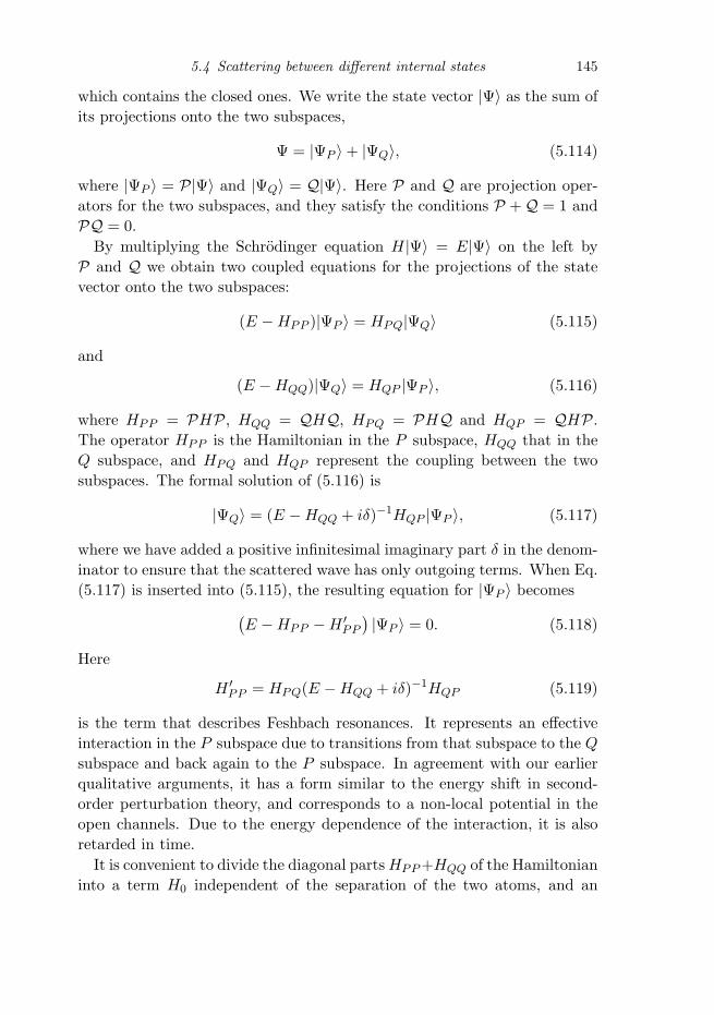
5.4 Scattering between different internal states 145
which contains the closed ones. We write the state vector |Ψ〉 as the sum ofits projections onto the two subspaces,
Ψ = |ΨP 〉 + |ΨQ〉, (5.114)
where |ΨP 〉 = P|Ψ〉 and |ΨQ〉 = Q|Ψ〉. Here P and Q are projection oper-ators for the two subspaces, and they satisfy the conditions P + Q = 1 andPQ = 0.
By multiplying the Schrodinger equation H|Ψ〉 = E|Ψ〉 on the left byP and Q we obtain two coupled equations for the projections of the statevector onto the two subspaces:
(E − HPP )|ΨP 〉 = HPQ|ΨQ〉 (5.115)
and
(E − HQQ)|ΨQ〉 = HQP |ΨP 〉, (5.116)
where HPP = PHP, HQQ = QHQ, HPQ = PHQ and HQP = QHP.The operator HPP is the Hamiltonian in the P subspace, HQQ that in theQ subspace, and HPQ and HQP represent the coupling between the twosubspaces. The formal solution of (5.116) is
|ΨQ〉 = (E − HQQ + iδ)−1HQP |ΨP 〉, (5.117)
where we have added a positive infinitesimal imaginary part δ in the denom-inator to ensure that the scattered wave has only outgoing terms. When Eq.(5.117) is inserted into (5.115), the resulting equation for |ΨP 〉 becomes(
E − HPP − H ′PP
)|ΨP 〉 = 0. (5.118)
Here
H ′PP = HPQ(E − HQQ + iδ)−1HQP (5.119)
is the term that describes Feshbach resonances. It represents an effectiveinteraction in the P subspace due to transitions from that subspace to the Q
subspace and back again to the P subspace. In agreement with our earlierqualitative arguments, it has a form similar to the energy shift in second-order perturbation theory, and corresponds to a non-local potential in theopen channels. Due to the energy dependence of the interaction, it is alsoretarded in time.
It is convenient to divide the diagonal parts HPP +HQQ of the Hamiltonianinto a term H0 independent of the separation of the two atoms, and an

146 Interactions between atoms
interaction contribution. Here H0 is the sum of the kinetic energy of therelative motion and the hyperfine and Zeeman terms, Eq. (3.8). We write
HPP = H0 + U1, (5.120)
where U1 is the interaction term for the P subspace. Equation (5.118) maybe rewritten as
(E − H0 − U) |ΨP 〉 = 0, (5.121)
where the total effective atom–atom interaction in the subspace of openchannels is given by
U = U1 + U2 (5.122)
with
U2 = H ′PP . (5.123)
A simple example
For the purpose of illustration, let us begin by considering the T matrix whenthere is no interaction in the open channels if the open and closed channelsare not coupled. This means that we set U1 = 0 in (5.120). We also treat U2
in the first Born approximation, which corresponds to equating the T matrixwith the matrix elements of U2 for plane-wave states. The diagonal elementof the T matrix in the channel αβ may be evaluated by using the identity1 =∑
n |n〉〈n|, where the states |n〉 form a complete set.7 If one takes for thestates the energy eigenstates in the absence of coupling between channels,the result for two atoms with zero relative momentum in the incoming state(labelled as |αβ, 0〉) is
〈αβ, 0|T |αβ, 0〉 =∑
n
|〈n|HQP |αβ, 0〉|2Eth(αβ) − En + iδ
, (5.124)
Here Eth(αβ) is the threshold energy (5.86), and we denote the eigenstatesof the Hamiltonian HQQ by En and the state vectors by |n〉. This result hasthe form anticipated, and it shows how the scattering length can be large ifthe energy of the two scattering particles is close to the energy of a state ina closed channel.
7 In the sum there are both bound states and continuum states. The normalization conditionfor the bound states is
∫dr|ψn(r)|2 = 1, and the continuum states are normalized as usual.

5.4 Scattering between different internal states 147
General solution
Before deriving more general results, we describe their key features. The ex-pression for the scattering length retains essentially the same form when theinteraction U1 is included, the only difference being that the open-channelplane-wave state |αβ, 0〉 is replaced by a scattering state which is an energyeigenstate of the Hamiltonian including the potential U1. When higher-order terms in U2 are taken into account, the energy of the resonant state isshifted, and the state may acquire a non-zero width due to decay to statesin the open channels.
To solve the problem more generally we calculate the T matrix corre-sponding to the interaction given in Eq. (5.118). As before, Eqs. (5.87) and(5.88), we write the Lippmann–Schwinger equation (5.45) as an operatorequation
T = U + UG0T. (5.125)
The quantity G0 is given by
G0 = (E − H0 + iδ)−1, (5.126)
where H0 is the Hamiltonian (5.81). It represents the free propagation ofatoms, and is the Green function for the Schrodinger equation. The formalsolution of (5.125) is
T = (1 − UG0)−1U = U(1 − G0U)−1. (5.127)
The second equality in (5.127) may be proved by multiplying (1−UG0)−1U
on the right by G0G−10 and using the fact that UG0 commutes with (1 −
UG0)−1, together with the identities
UG0(1 − UG0)−1G−10 = U [G0(1 − UG0)G−1
0 ]−1 = U(1 − G0U)−1. (5.128)
By inserting (5.126) into the first equality in (5.127) we obtain
T = (E + iδ − H0)(E + iδ − H0 − U)−1U. (5.129)
Putting A = E + iδ − H0 − U1 and B = U2 in the matrix identity
(A − B)−1 = A−1(1 + B(A − B)−1) (5.130)
one finds
(E+iδ−H0−U)−1 = (E+iδ−H0−U1)−1[1+U2(E+iδ−H0−U)−1], (5.131)
which when inserted into Eq. (5.129) gives the useful result
T = T1 + (1 − U1G0)−1U2(1 − G0U)−1. (5.132)

148 Interactions between atoms
Here T1, which satisfies the equation T1 = U1 + U1G0T1, is the T matrix inthe P subspace if transitions to the Q subspace are neglected.
Let us now interpret the result (5.132) by considering its matrix elementsbetween plane-wave states with relative momenta k and k′:
〈k′|T |k〉 = 〈k′|T1|k〉 + 〈k′|(1 − U1G0)−1U2(1 − G0U)−1|k〉. (5.133)
The scattering amplitude is generally a matrix labelled by the quantumnumbers of the entrance and exit channels, but for simplicity we suppress theindices. Acting on a plane-wave state for the relative motion |k〉 the operatorΩU = (1 − G0U)−1 generates an eigenstate of the Hamiltonian H0 + U , asone may verify by operating on the state with the Hamiltonian. This result isequivalent to Eqs. (5.41) and (5.42) for the single-channel problem. At largeseparations the state ΩU |k〉 consists of a plane wave and a spherical wave,which is outgoing because of the iδ in G0. We denote this state by |k; U, +〉,the plus sign indicating that the state has outgoing spherical waves. Theoperators U1 and H0 are Hermitian and therefore (1 − U1G0)† = 1 − G−
0 U1
for E real, where G−0 = (E − H0 − iδ)−1 is identical with G0 defined in Eq.
(5.126) except that the sign of the infinitesimal imaginary part is opposite.We may thus write
〈k′|(1 − U1G0)−1 = [(1 − G−0 U1)−1|k′〉]† ≡ [|k′; U1,−〉]†. (5.134)
As a consequence of the difference of the sign of δ, the state contains incom-ing spherical waves at large distances, and this is indicated by the minussign in the notation for the eigenstates.8 The scattering amplitude (5.133)may therefore be written as
〈k′|T |k〉 = 〈k′|T1|k〉 + 〈k′; U1,−|U2|k; U, +〉. (5.135)
This is the general expression for the scattering amplitude in the P subspace.
Tuning effective interactions
We now apply the above results, and we begin by considering the contri-bution of first order in U2. This is equivalent to replacing U by U1 in Eq.(5.133), which gives
T � T1 + (1 − U1G0)−1U2(1 − G0U1)−1. (5.136)
8 If the relative velocity of the incoming particles is zero and provided real scattering betweendifferent open channels may be neglected, scattering states with ‘outgoing’ spherical waves arethe same as those with ‘incoming’ ones since there are no phase factors of the form e±ikr, andtherefore both functions behave as 1 − a/r at large distances.

5.4 Scattering between different internal states 149
The matrix elements between plane-wave states are given by
〈k′|T |k〉 = 〈k′|T1|k〉 + 〈k′; U1,−|U2|k; U1, +〉. (5.137)
This result differs from the simple example with U1 = 0 that we consideredabove in two respects: the interaction in the P subspace gives a contribu-tion T1 to the T matrix, and the contribution due to the U2 term is to beevaluated using scattering states that take into account the potential U1,not plane waves.
Let us now neglect coupling between the open channels. The scattering ina particular channel for particles with zero relative velocity is then specifiedby the scattering length, which is related to the T matrix by the usual factor.As explained in footnote 7, we may then neglect the difference between thescattering states with incoming and outgoing spherical waves and we shalldenote the state simply by |ψ0〉. We again evaluate the matrix element ofU2, defined in Eqs. (5.119) and (5.123), by inserting the unit operator andfind
4π�2
ma =
4π�2
maP +
∑n
|〈ψn|HQP |ψ0〉|2Eth − En
, (5.138)
where the sum is over all states in the Q subspace and aP is the scatteringlength when coupling between open and closed channels is neglected.
If the energy Eth is close to the energy Eres of one particular bound state,contributions from all other states will vary slowly with energy, and they,together with the contribution from the potential U1, may be representedby a non-resonant scattering length anr whose energy dependence may beneglected. However in the resonance term the energy dependence must beretained. The scattering length may then be written as
4π�2
ma =
4π�2
manr +
|〈ψres|HQP |ψ0〉|2Eth − Eres
. (5.139)
This displays the energy dependence characteristic of a Feshbach resonance.Atomic interactions may be tuned by exploiting the fact that the energies
of states depend on external parameters, among which are the strengths ofmagnetic and electric fields. For definiteness, let us consider an externalmagnetic field. We imagine that the energy denominator in Eq. (5.139)vanishes for a particular value of the magnetic field, B = B0. Expandingthe energy denominator about this value of the magnetic field we find
Eth − Eres � (μres − μα − μβ)(B − B0), (5.140)

150 Interactions between atoms
where
μα = −∂εα
∂Band μβ = −∂εβ
∂B(5.141)
are the magnetic moments of the two atoms in the open channel, and
μres = −∂Eres
∂B(5.142)
is the magnetic moment of the molecular bound state. The scattering lengthis therefore given by
a = anr
(1 − ΔB
B − B0
)(5.143)
where the width parameter ΔB is given by
ΔB =m
4π�2anr
|〈ψres|HQP |ψ0〉|2(μα + μβ − μres)
. (5.144)
At a magnetic field B = B0 + ΔB the scattering length vanishes. Note thatthe strength of the divergence in a is measured by the combination anrΔB,which is finite in the limit anr → 0. This shows that the characteristic rangeof magnetic fields over which the resonance significantly affects the scatteringlength depends on the magnetic moments of the states, and on the couplingbetween channels. Consequently, measurement of Feshbach resonances pro-vides a means of obtaining information about interactions between atoms.Equation (5.143) shows that in this approximation the scattering length di-verges to ±∞ as B approaches B0. Because of the dependence on 1/(B−B0),large changes in the scattering length can be produced by small changes inthe field. It is especially significant that the sign of the interaction can bechanged by a small change in the field.
Higher-order contributions in U2 may be included, and the exact solution(5.133) may be expressed in the form
T = T1 +(1−U1G0)−1HPQ(E−HQQ−H ′QQ)−1HQP (1−G0U1)−1, (5.145)
where
H ′QQ = HQP (E − HPP )−1HPQ. (5.146)
By comparing this result with the earlier one (5.136) we see that the onlyeffect of higher-order terms in U2 is to introduce an extra contribution H ′
in the Hamiltonian acting in the Q subspace. This effective interactionin the Q subspace takes into account the influence of coupling to the openchannels, and it is therefore the analogue of the interaction H ′
PP in the openchannels. Physically it has two effects. One is to shift the energies of the

5.5 Determination of scattering lengths 151
bound states, and the second is to give them a non-zero width �Γres if decayinto open channels is possible. The width leads to a scattering amplitude ofthe Breit–Wigner form ∝ 1/(Eth −Eres + i�Γres/2). For |Eth −Eres| �Γres
the scattering amplitude shows the 1/(Eth−Eres) behaviour predicted by thesimpler calculations. For |Eth − Eres| � �Γres the divergence is cut off andthe scattering amplitude behaves smoothly. However, the width of resonantstates close to the threshold energy in the open channel is generally verysmall because of the small density of final states, and Feshbach resonancesfor cold atoms are consequently very sharp.
Detailed calculations of Feshbach resonances have been made for lithiumand sodium, using the methods outlined above, by Moerdijk et al. [18].Feshbach resonances have been investigated experimentally for a variety ofatoms, including 23Na [19], 85Rb [20,21], 133Cs [4] and 6Li [22]. Level shiftsdue to the interaction of atoms with a laser field can also induce Feshbachresonances, as has been observed in sodium [23]. As we shall describe in Sec.5.5, Feshbach resonances are a key tool for extracting information about in-teractions between atoms. In addition they provide a means of varying thescattering length almost at will, and this allows one to explore propertiesof condensates under novel conditions. For example, in the experiment byCornish et al. on 85Rb described in Ref. [21] the effective interaction waschanged from positive to negative by varying the magnetic field, and thiscaused the cloud to collapse. In Chapter 17 we discuss the role of Feshbachresonances in the production of cold molecules and the study of the crossoverbetween Bose–Einstein condensation and Bardeen–Cooper–Schrieffer pair-ing.
5.5 Determination of scattering lengths
In this section we survey the methods used to determine scattering lengthsof alkali atoms. Most experiments do not give directly the value of thescattering length, but they give information about atom–atom interactions,from which scattering lengths may be calculated. The general framework inwhich this is done was described immediately preceding Sec. 5.4.1.
Measurement of the collision cross section
For identical bosons, the cross section for elastic collisions at low energyis given by 8πa2, and therefore a measurement of the elastic cross sectiongives the magnitude of the scattering length, but not its sign. In Sec. 11.3we shall describe how the scattering length is related to the damping rate

152 Interactions between atoms
S + S
S + P
Energy
Atomic separation
Fig. 5.5 Schematic representation of potential energy curves to illustrate themethod of photoassociative spectroscopy.
for collective modes and temperature anisotropies. One difficulty of thistechnique is that it requires knowledge of the particle density.
Molecular spectra
Measurements of the frequencies of transitions between molecular boundstates of two polarized atoms give information about the interaction po-tential. However, this method is not particularly sensitive to the long-rangepart of the interaction, which is crucial for determining the scattering length.
Photoassociative spectroscopy
The understanding of interactions between cold atoms has been advancedsignificantly by the use of photoassociative spectroscopy, in which one mea-sures the rate at which two interacting ground-state atoms in an unboundstate are excited by means of a laser to a molecular state in which one of theatoms is in a P state. The principle of the method is illustrated in Fig. 5.5.For two atoms in the ground state, the potential is of the van der Waals form(∝ r−6) at large distances, as described in Sec. 5.1. This is represented bythe lower curve, labelled ‘S+S’. When one atom is excited to a P state, theelectric dipole–dipole interaction, Eq. (5.3), gives a first-order contributionto the energy because the state with one atom excited and the other in the

5.5 Determination of scattering lengths 153
ground state is degenerate with the state in which the two atoms are inter-changed, and this varies as r−3 at large distances, as does the dipole–dipoleinteraction itself. Its sign can be either positive or negative, depending onthe symmetry of the excited state of the two atoms. The potentials for thiscase are labelled in the figure by ‘S + P’.
The long-range part of the potential when one atom is excited is very muchstronger than the van der Waals interaction and, consequently, the excited-state potential, when attractive, has many bound states, some of whichhave sizes much greater than those of the bound states for the ground-statepotential. The transition rate to an excited molecular state is given in termsof the matrix element of the perturbation due to the laser, between the statewith two ground-state atoms and the excited state. The spatial variation ofthe ground-state wave function is generally slow compared with that of theexcited molecular state, since the excited-state potential is much stronger.Consequently, the largest contribution to the matrix element comes fromthe region where the relative momentum of the two atoms in the excitedstate is small, that is near the classical turning points of the motion. Inregions where the relative momentum is larger, the product of the two wavefunctions oscillates rapidly in space, and, when integrated over space, giveslittle contribution to the matrix element. Thus the transition probabilitydepends sensitively on the magnitude of the ground-state wave function nearthe turning point of the motion in the excited molecular state. The positionof the turning point depends on the molecular state under consideration, andtherefore the variation of the strengths of transitions to different molecularstates, which have different energies and are therefore resonant at differentlaser frequencies, shows strong features due to the oscillations in the ground-state wave function for two atoms. From a knowledge of the excited-statepotential and the transition rates for a number of molecular excited statesit is possible to deduce properties of the ground-state wave function andscattering length.
Excited molecular states may decay to give atoms which have kinetic ener-gies high enough that they can overcome the trapping potential. Therefore,one way of detecting transitions to excited molecular states is by measuringtrap loss. Alternatively, a second light pulse may be used to excite the atomfurther, possibly to an ionized state which is easily detectable. Extensivediscussions of the method and developments of it are given in Refs. [1] and[2].

154 Interactions between atoms
Other methods
Other measurements give information about atomic interactions. Since ratesof inelastic processes are sensitive to the atomic interaction, especially todifferences between singlet and triplet scattering lengths, measurement ofthem can give information about the potential. This has been particularlyimportant for 87Rb. Surprisingly, it was found experimentally that a cloudwith two condensates, one in the F = 2, mF = 2 state and the other inthe F = 1, mF = −1 state, lived much longer than suggested by an order-of-magnitude estimate of the lifetime due to exchange collisions based onEq. (5.103) with the assumption that |at − as| is comparable to |at|. Theexplanation for this is that the triplet and singlet scattering lengths arenearly equal. This means physically that the singlet and triplet componentsof the wave function are essentially in phase again when the two particleshave been scattered, and consequently they reconstruct the initial hyperfinestate, with only a small admixture of other hyperfine states.
As explained in Sec. 5.4.2, the positions of Feshbach resonances and thewidth ΔB, Eq. (5.144), are sensitive to the interatomic interaction. There-fore by studying these resonances it is possible to deduce properties of in-teratomic potentials. Techniques that make use of Feshbach resonances areimportant in extracting information about potentials, as is exemplified bythe discussion of results for Rb isotopes and 133Cs given below.
5.5.1 Scattering lengths for alkali atoms and hydrogen
Below we list values of the scattering lengths in zero magnetic field forhydrogen and the members of the alkali series.9 The reader is referred to Ref.[2] and the original literature for further discussion. The triplet scatteringlength is denoted by at, the singlet one by as, and that for two atoms in themaximally stretched lower hyperfine state F = I − 1/2, mF = −(I − 1/2)by ams. All scattering lengths are given in atomic units (1 a.u. = a0 =4πε0�
2/mee2 ≈ 0.0529 nm).
Hydrogen
The hydrogen atom is sufficiently simple that scattering lengths may becalculated reliably from first principles, with the results at = 1.2 [24] andas = 0.41 [25].
9 Due to the existence of Feshbach resonances, scattering lengths in the presence of a magneticfield can differ considerably from the zero-field values.

5.5 Determination of scattering lengths 155
Lithium
6Li For this fermion Abraham et al. [26], who employed photoassociativespectroscopy, obtained as = 45.5 ± 2.5 and at = −2160 ± 250, the latterexceeding by more than one order of magnitude the estimate based on thedimensional arguments of Sec. 5.1. More recently, accurate determinationof the parameters by the use of radio-frequency spectroscopy led to as =45.167 ± 0.008 and at = −2140 ± 18 [22].
7Li The work of Ref. [26] led to the values as = 33±2 and at = −27.6±0.5.As we shall see in Chapter 6, the negative value of the triplet scatteringlength for 7Li prevents the formation of a condensate with more than a fewthousand atoms.
Sodium23Na Scattering lengths have been derived by Tiesinga et al. [27] fromphotoassociative spectroscopy data. They found at = 85 ± 3 and ams =52±5. A more recent analysis of different types of data gives at = 65.3±0.9,as = 19.1 ± 2.1, and ams = 55.4 ± 1.2 [28].
Potassium
Scattering lengths for potassium isotopes have been derived from photoas-sociative spectroscopy by Bohn et al. [29]. Their results are:
39K at = −17 ± 25, as = 140+3−6, and ams = −20+42
−64,
40K at = 194+114−35 and as = 105+2
−3,
41K at = 65+13−8 , as = 85 ± 2, and ams = 69+14
−9 .
These values are somewhat different from earlier ones obtained from molec-ular spectroscopy [30,31].
Rubidium85Rb From photoassociative spectroscopy and study of a Feshbach reso-nance, Roberts et al. found at = −369 ± 16 and as = 2400+600
−350 [21]. Vogelset al. found ams = −450 ± 140 from photoassociative spectroscopy [32].
87Rb All the scattering lengths are closely equal. Roberts et al. foundat = 106 ± 4 and as = 90 ± 1 from the same kinds of data as they used for

156 Interactions between atoms
the lighter isotope [21]. From measurements of the lifetime of two coexistingcondensates and from photoassociative spectroscopy Julienne et al. foundams = 103 ± 5 [33].
Cesium133Cs The scattering cross section of 133Cs atoms in the doubly polarizedstate, F = 4, mF = 4, was measured by Arndt et al. [34] in the temperaturerange from 5 to 60 μK. It was found to be inversely proportional to thetemperature, characteristic of resonant scattering (|a| → ∞). Since the crosssection did not saturate at the lowest temperatures, the measurements yieldonly a lower bound on the magnitude of the scattering length, |at| ≥ 260.Chin et al. [4] have made high-resolution measurements of a large numberof Feshbach resonances, from which Leo et al. [5] deduced the values at =2400 ± 100 and as = 280 ± 10. Because of the many resonances, scatteringlengths depend sensitively on the magnetic field.
Problems
Problem 5.1 Use the model of Sec. 5.3 to determine the value of rc/r0 atwhich the first bound state appears. In the light of this calculation, discusswhy two spin-polarized hydrogen atoms in a triplet electronic state do nothave a bound state. (The triplet-state potential for hydrogen is positive fordistances less than approximately 7a0.)
Problem 5.2 Calculate the rate of the process d + d → a + a for hy-drogen atoms at zero temperature. This process was discussed in Sec. 4.7,and expressions for the states are given in Eqs. (3.24)–(3.27). Use the Bornapproximation and take into account only the magnetic dipole–dipole inter-action. Give limiting results for low magnetic fields (B ΔEhf/μB) andhigh magnetic fields.
Problem 5.3 Make numerical estimates of rates of elastic scattering, andinelastic two- and three-body processes for hydrogen and alkali atoms at lowtemperatures under typical experimental conditions.
References[1] J. Weiner, V. S. Bagnato, S. Zilio, and P. S. Julienne, Rev. Mod. Phys. 71, 1
(1999).[2] D. J. Heinzen, in Bose–Einstein Condensation in Atomic Gases, Proceedings

References 157
of the Enrico Fermi International School of Physics, Vol. CXL, ed. M.Inguscio, S. Stringari, and C. E. Wieman, (Amsterdam, IOS Press, 1999),p. 351.
[3] A. Derevianko, J. F. Babb, and A. Dalgarno, Phys. Rev. A 63, 052704 (2001).[4] C. Chin, V. Vuletic, A. J. Kerman, and S. Chu, Phys. Rev. Lett. 85, 2717
(2000).[5] P. J. Leo, C. J. Williams, and P. S. Julienne, Phys. Rev. Lett. 85, 2721
(2000).[6] L. D. Landau and E. M. Lifshitz, Quantum Mechanics, Third edition, (New
York, Pergamon, 1977).[7] See, e.g., K. Huang, Statistical Mechanics, Second Edition, (New York,
Wiley, 1987), p. 233.[8] G. F. Gribakin and V. V. Flambaum, Phys. Rev. A 48, 546 (1993).[9] G. V. Shlyapnikov, J. T. M. Walraven, and E. L. Surkov, Hyp. Int. 76, 31
(1993).[10] H. T. C. Stoof, J. M. V. A. Koelman, and B. J. Verhaar, Phys. Rev. B 38,
4688 (1988).[11] A. J. Moerdijk and B. J. Verhaar, Phys. Rev. A 53, 19 (1996).[12] F. H. Mies, C. J. Williams, P. S. Julienne, and M. Krauss, J. Res. Natl. Inst.
Stand. Technol. 101, 521 (1996).[13] A. J. Moerdijk, H. M. J. M. Boesten, and B. J. Verhaar, Phys. Rev. A 53,
916 (1996).[14] H. Feshbach, Ann. Phys. 19, 287 (1962).[15] U. Fano, Phys. Rev. 124, 1866 (1961).[16] W. C. Stwalley, Phys. Rev. Lett. 37, 1628 (1976).[17] T. Kohler, K. Goral, and P. S. Julienne, Rev. Mod. Phys. 78, 1311 (2006).[18] A. J. Moerdijk, B. J. Verhaar, and A. Axelsson, Phys. Rev. A 51, 4852
(1995).[19] S. Inouye, M. R. Andrews, J. Stenger, H.-J. Miesner, D. M. Stamper-Kurn,
and W. Ketterle, Nature 392, 151 (1998).[20] P. Courteille, R. S. Freeland, D. J. Heinzen, F. A. van Abeelen, and
B. J. Verhaar, Phys. Rev. Lett. 81, 69 (1998).[21] J. L. Roberts, N. R. Claussen, J. P. Burke, C. H. Greene, E. A. Cornell, and
C. A. Wieman, Phys. Rev. Lett. 81, 5109 (1998); S. L. Cornish, N. R.Claussen, J. L. Roberts, E. A. Cornell, and C. A. Wieman, Phys. Rev. Lett.85, 1795 (2000).
[22] M. Bartenstein, A. Altmeyer, S. Riedl, R. Geursen, S. Jochim, C. Chen, J. H.Denschlag, R. Grimm, A. Simoni, E. Tiesinga, C. J. Williams, and P. S.Julienne, Phys. Rev. Lett. 94, 103201 (2005).
[23] F. K. Fatemi, K. M. Jones, and P. D. Lett, Phys. Rev. Lett. 85, 4462 (2000).[24] M. J. Jamieson, A. Dalgarno, and M. Kimura, Phys. Rev. A 51, 2626 (1995).[25] M. J. Jamieson, A. Dalgarno, and J. N. Yukich, Phys. Rev. A 46, 6956
(1992).

158 Interactions between atoms
[26] E. R. I. Abraham, W. I. McAlexander, J. M. Gerton, R. G. Hulet, R. Cote,and A. Dalgarno, Phys. Rev. A 55, 3299 (1997).
[27] E. Tiesinga, C. J. Williams, P. S. Julienne, K. M. Jones, P. D. Lett, andW. D. Phillips, J. Res. Nat. Inst. Stand. Technol. 101, 505 (1996).
[28] F. A. van Abeelen and B. J. Verhaar, Phys. Rev. A 59, 578 (1999).[29] J. L. Bohn, J. P. Burke, C. H. Greene, H. Wang, P. L. Gould, and
W. C. Stwalley, Phys. Rev. A 59, 3660 (1999).[30] H. M. J. M. Boesten, J. M. Vogels, J. G. C. Tempelaars, and B. J. Verhaar,
Phys. Rev. A 54, 3726 (1996).[31] R. Cote, A. Dalgarno, H. Wang, and W. C. Stwalley, Phys. Rev. A 57, 4118
(1998).[32] J. M. Vogels, C. C. Tsai, R. S. Freeland, S. J. J. M. F. Kokkelmans,
B. J. Verhaar, and D. J. Heinzen, Phys. Rev. A 56, 1067 (1997).[33] P. S. Julienne, F. H. Mies, E. Tiesinga, and C. J. Williams, Phys. Rev. Lett.
78, 1880 (1997).[34] M. Arndt, M. Ben Dahan, D. Guery-Odelin, M. W. Reynolds, and
J. Dalibard, Phys. Rev. Lett. 79, 625 (1997).

QUERIES TO BE ANSWERED BY AUTHOR (SEE MARGINALMARKS)
IMPORTANT NOTE: Please mark your corrections and an-swers to these queries directly onto the proof at the relevantplace. Do NOT mark your corrections on this query sheet.
Chapter 05
Q. No. Pg No. QueryAQ1 129 Please check the corrections made
on this sentence

6
Theory of the condensed state
In the present chapter we consider the structure of the Bose–Einstein con-densed state in the presence of interactions. Our discussion is based on theGross–Pitaevskii equation [1], which describes the zero-temperature prop-erties of the non-uniform Bose gas when the scattering length a is muchless than the mean interparticle spacing. We shall first derive the Gross–Pitaevskii equation at zero temperature by treating the interaction betweenparticles in a mean-field approximation (Sec. 6.1). Following that, in Sec.6.2 we discuss the ground state of atomic clouds in a harmonic-oscillatorpotential. We compare results obtained by variational methods with thosederived in the Thomas–Fermi approximation, in which the kinetic energyoperator is neglected in the Gross–Pitaevskii equation. The Thomas–Fermiapproximation fails near the surface of a cloud, and in Sec. 6.3 we calcu-late the surface structure using the Gross–Pitaevskii equation. In Sec. 6.4we determine how the condensate wave function ‘heals’ when subjected to alocalized disturbance. Finally, in Sec. 6.5 we show how the magnetic dipole–dipole interaction, which is long-ranged and anisotropic, may be includedin the Gross–Pitaevskii equation and determine within the Thomas–Fermiapproximation its effect on the density distribution.
6.1 The Gross–Pitaevskii equation
In the previous chapter we have shown that the effective interaction betweentwo particles at low energies is a constant in the momentum representation,U0 = 4π�
2a/m. In coordinate space this corresponds to a contact interac-tion U0δ(r − r′), where r and r′ are the positions of the two particles. Toinvestigate the energy of many-body states we adopt a Hartree or mean-fieldapproach, and assume that the wave function is a symmetrized product ofsingle-particle wave functions. In the fully condensed state, all bosons are
159

160 Theory of the condensed state
in the same single-particle state, φ(r), and therefore we may write the wavefunction of the N -particle system as
Ψ(r1, r2, . . . , rN ) =N∏
i=1
φ(ri). (6.1)
The single-particle wave function φ(ri) is normalized in the usual way,∫dr|φ(r)|2 = 1. (6.2)
This wave function does not contain the correlations produced by the inter-action when two atoms are close to each other. These effects are taken intoaccount by using the effective interaction U0δ(r − r′), which includes theinfluence of short-wavelength degrees of freedom that have been eliminated,or integrated out, as described in Sec. 5.2.1. In the mean-field treatment,we shall take into account explicitly interactions between degrees of freedomcorresponding to length scales such as the spatial extent of the cloud, thescale of surface structure, or the wavelength of an excitation. These lengthscales are generally much larger than the lengths associated with scattering,r0 given by Eq. (5.1) and the magnitude of the scattering length. Thereforewe may generally set the cut-off wave number kc to zero.1 The effective in-teraction is thus equal to U0, the T matrix at zero energy, and the effectiveHamiltonian may be written
H =N∑
i=1
[p2
i
2m+ V (ri)
]+ U0
∑i<j
δ(ri − rj), (6.3)
V (r) being the external potential. The energy of the state (6.1), the expec-tation value of the Hamiltonian (6.3) in the state, is given by
E = N
∫dr[
�2
2m|∇φ(r)|2 + V (r)|φ(r)|2 +
(N − 1)2
U0|φ(r)|4]. (6.4)
In the interaction term, N(N − 1)/2 is the number of terms in the inter-action energy, that is the number of ways of making pairs of bosons, times∫
drU0|φ(r)|4, the interaction energy of two particles in the state φ(r).2
In the Hartree approximation, all atoms are in the state whose wave func-tion we denote by φ. In the true wave function, some atoms will be in stateswith more rapid spatial variation, due to the correlations at small atomicseparations, and therefore the total number of atoms in the state φ will be1 An exception is the calculation of the depletion of the condensate in Sec. 8.1.3.2 For a more general two-particle interaction U(r, r′), the interaction energy of two particles both
in the state φ(r) is∫
drdr′U(r, r′)|φ(r)|2|φ(r′)|2.
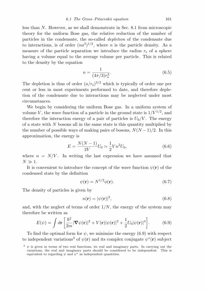
6.1 The Gross–Pitaevskii equation 161
less than N . However, as we shall demonstrate in Sec. 8.1 from microscopictheory for the uniform Bose gas, the relative reduction of the number ofparticles in the condensate, the so-called depletion of the condensate dueto interactions, is of order (na3)1/2, where n is the particle density. As ameasure of the particle separation we introduce the radius rs of a spherehaving a volume equal to the average volume per particle. This is relatedto the density by the equation
n =1
(4π/3)r3s
. (6.5)
The depletion is thus of order (a/rs)3/2 which is typically of order one percent or less in most experiments performed to date, and therefore deple-tion of the condensate due to interactions may be neglected under mostcircumstances.
We begin by considering the uniform Bose gas. In a uniform system ofvolume V , the wave function of a particle in the ground state is 1/V 1/2, andtherefore the interaction energy of a pair of particles is U0/V . The energyof a state with N bosons all in the same state is this quantity multiplied bythe number of possible ways of making pairs of bosons, N(N − 1)/2. In thisapproximation, the energy is
E =N(N − 1)
2VU0 � 1
2V n2U0, (6.6)
where n = N/V . In writing the last expression we have assumed thatN 1.
It is convenient to introduce the concept of the wave function ψ(r) of thecondensed state by the definition
ψ(r) = N1/2φ(r). (6.7)
The density of particles is given by
n(r) = |ψ(r)|2, (6.8)
and, with the neglect of terms of order 1/N , the energy of the system maytherefore be written as
E(ψ) =∫
dr[
�2
2m|∇ψ(r)|2 + V (r)|ψ(r)|2 +
12U0|ψ(r)|4
]. (6.9)
To find the optimal form for ψ, we minimize the energy (6.9) with respectto independent variations3 of ψ(r) and its complex conjugate ψ∗(r) subject3 ψ is given in terms of two real functions, its real and imaginary parts. In carrying out the
variations, the real and imaginary parts should be considered to be independent. This isequivalent to regarding ψ and ψ∗ as independent quantities.

162 Theory of the condensed state
to the condition that the total number of particles
N =∫
dr|ψ(r)|2 (6.10)
be constant. The constraint is conveniently taken care of by the methodof Lagrange multipliers. One writes δE − μδN = 0, where the chemicalpotential μ is the Lagrange multiplier that ensures constancy of the particlenumber and the variations of ψ and ψ∗ may thus be taken to be arbitrary.This procedure is equivalent to minimizing the quantity E − μN at fixed μ.Equating to zero the variation of E − μN with respect to ψ∗(r) gives
− �2
2m∇2ψ(r) + V (r)ψ(r) + U0|ψ(r)|2ψ(r) = μψ(r), (6.11)
To obtain this result, the variation of the kinetic energy term was carriedout by performing an integration by parts. The surface terms that arise inthis process vanish for systems of finite extent or when periodic boundaryconditions are imposed. Equation (6.11) is the time-independent Gross–Pitaevskii equation. It has the form of a Schrodinger equation in which thepotential acting on particles is the sum of the external potential V and anon-linear term U0|ψ(r)|2 that takes into account the mean field producedby the other bosons.4 Note that the eigenvalue is the chemical potential, notthe energy per particle as it is for the usual (linear) Schrodinger equation.For non-interacting particles all in the same state the chemical potential isequal to the energy per particle, but for interacting particles it is not.
For a uniform Bose gas, the Gross–Pitaevskii equation (6.11) is
μ = U0|ψ(r)|2 = U0n, (6.12)
which agrees with the result of using the thermodynamic relation μ =∂E/∂N to calculate the chemical potential from the energy of the uniformstate, Eq. (6.6).
6.2 The ground state for trapped bosons
We now examine the solution of the Gross–Pitaevskii equation for bosonsin a trap [2]. For definiteness, and because of their experimental relevance,4 In the Gross–Pitaevskii approximation, the interaction energy of an atom at position r is given
by the density of other atoms at that point times the effective interaction. This approach istherefore closely related to Landau’s theory of normal Fermi liquids. It must be contrastedwith the Hartree approximation used for atoms, and with mean-field theory as applied to high-density degenerate plasmas or lattice magnetic systems with high coordination number, wherecorrelations are unimportant and the potential energy is given directly in terms of the bareinteraction. Correlations are important in dilute Bose gases, and their effects are taken intoaccount by using the effective interaction, rather than the bare one.

6.2 The ground state for trapped bosons 163
we shall consider harmonic traps, but the formalism may easily be appliedto more general traps.
Before embarking on detailed calculations let us consider qualitative prop-erties of the solution. For simplicity, we neglect the anisotropy of the oscil-lator potential, and take it to be of the form V = mω2
0r2/2. If the spatial
extent of the cloud is ∼ R, the potential energy of a particle in the oscillatorpotential is ∼ mω2
0R2/2, and the kinetic energy is of order �
2/2mR2 perparticle, since in the ground state a typical particle momentum is of order�/R from the Heisenberg uncertainty principle. Thus in the absence of in-teractions, the total energy varies as 1/R2 for small R and as R2 for largeR, and it has a minimum when the kinetic and potential energies are equal.The corresponding value of the radius of the cloud is of order
aosc =(
�
mω0
)1/2
, (6.13)
which is the characteristic quantum-mechanical length scale for the harmonicoscillator. This result is what one would anticipate, because we have madewhat amounts to a variational calculation of the ground state of a singleparticle in an oscillator potential.
We now consider the effect of interactions. A typical particle densityis n ∼ N/R3, and the interaction energy of a particle is therefore of or-der nU0 ∼ U0N/R3. For repulsive interactions, the effect of an additionalcontribution to the energy varying as R−3 shifts the minimum of the totalenergy to larger values of R, and consequently, for increasing values of Na,the kinetic energy term becomes less important. It is instructive to inves-tigate the limit of strong interactions, in which the kinetic energy may beneglected. The equilibrium size is found by minimizing the sum of the po-tential and interaction energies, and this occurs when the two contributionsto the energy are of the same order of magnitude. By equating the twoenergies, one finds the equilibrium radius to be given by
R ∼ aosc
(Naaosc
)1/5
, (6.14)
and the energy per particle is
E
N∼ �ω0
(Naaosc
)2/5
. (6.15)
The quantity Na/aosc is a dimensionless measure of the strength of the in-teraction, and in most experiments on atoms with repulsive interactions itis much larger than unity, so the radius R is somewhat larger than aosc. For

164 Theory of the condensed state
|a| ∼ 10 nm and aosc ∼ 1 μm (see Eq. (2.35)), with N between 104 and106, the ratio R/aosc is seen to range from 2.5 to 6. In equilibrium, theinteraction energy and the energy due to the trapping potential are both oforder mω2
0R2, where R is the equilibrium radius given by (6.14), and there-
fore the ratio between the kinetic energy, which is proportional to R−2, andthe other contributions to the energy is proportional to (aosc/Na)4/5. Thisconfirms that the kinetic energy is indeed negligible for clouds containing asufficiently large number of particles.5
Let us now turn to attractive interactions. For a small number of parti-cles, the total energy as a function of R is similar to that for non-interactingparticles, except that at very small R the energy diverges to −∞ as −1/R3.Consequently, for a sufficiently small number of particles the energy hasa local minimum near that for non-interacting particles, but at a smallerradius. This state is metastable, since for small departures from the mini-mum, the energy increases, but for small R the energy eventually varies as−1/R3 and becomes less than that at the local minimum. With increasingparticle number, the local minimum becomes shallower, and at a criticalparticle number Nc it disappears. For larger numbers of particles there isno metastable state. As one might expect, the critical number is determinedby the condition that the dimensionless coupling parameter be of order −1,that is Nc ∼ aosc/|a|. For two 7Li atoms in the F = 2, mF = 2 state, theelectronic state is a triplet, and the scattering length at is −27.6a0 = −1.46nm. Therefore in traps with frequencies of order 100 Hz, corresponding toaosc of order microns, the critical number is of order 103, which is what isfound experimentally [3].
We now consider the problem quantitatively. We shall determine theground-state energy for a gas trapped in an anisotropic three-dimensionalharmonic-oscillator potential V given by
V (x, y, z) =12m(ω2
xx2 + ω2yy
2 + ω2zz
2), (6.16)
where the three oscillator frequencies ωi (i = x, y, z) may differ from eachother. Many traps used in experiments have an axis of symmetry, so thattwo of the frequencies are equal, but we shall consider the general case.The Gross–Pitaevskii equation (6.11) may be solved directly by numericalintegration, but it is instructive to derive some analytical results. We beginwith a variational calculation based on a Gaussian trial function and thengo on to the Thomas–Fermi approximation.
5 As we shall see from the detailed calculations in Sec. 6.3, the leading term is of order(aosc/Na)4/5 ln(Na/aosc).

6.2 The ground state for trapped bosons 165
6.2.1 A variational calculation
In the absence of interparticle interactions the lowest single-particle statehas the familiar wave function,
φ0(r) =1
π3/4(axayaz)1/2e−x2/2a2
xe−y2/2a2ye−z2/2a2
z , (6.17)
where the oscillator lengths ai (i = x, y, z) are given by a2i = �/mωi accord-
ing to Eq. (2.34). The density distribution n(r) = Nφ0(r)2 is thus Gaussian.Interatomic interactions change the dimensions of the cloud, and we adoptas our trial function for ψ the same form as (6.17),
ψ(r) =N1/2
π3/4(bxbybz)1/2e−x2/2b2xe−y2/2b2ye−z2/2b2z , (6.18)
where the lengths bi are variational parameters. The trial function satisfiesthe normalization condition (6.10). Substitution of (6.18) into (6.9) yieldsthe energy expression
E(bx, by, bz) = N∑
i
�ωi
(a2
i
4b2i
+b2i
4a2i
)+
N2U0
2(2π)3/2bxbybz. (6.19)
If we evaluate (6.19), putting the bi equal to their values ai in the absenceof interaction, one finds
E � N∑
i
�ωi
2+
N2U0
2(2π)3/2axayaz
= N∑
i
�ωi
2+
N2
2〈00|v|00〉, (6.20)
where
〈00|v|00〉 =4π�
2a
m
∫dr|φ0(r)|4 (6.21)
is the interaction energy for two particles in the ground state of the oscillator.The result (6.20) is valid to first order in a, and it is a good approximationas long as the interaction energy per particle is small compared with thesmallest of the zero-point energies �ωi/2. If the magnitudes of the threeoscillator frequencies are comparable (ωi ∼ ω0), the ratio of the interactionenergy to the zero-point energy of the oscillator is of order Na/aosc, which,as we argued above, is a dimensionless measure of the strength of the inter-action. It gives the ratio of the interaction energy to the oscillator energy�ω0 when the wave function is that for the particles in the ground stateof the oscillator. The condition Na/aosc ∼ 1 marks the crossover between

166 Theory of the condensed state
the perturbative regime and one where equilibrium is determined by com-petition between the interaction energy and the potential energy due to thetrap.
With increasing positive effective interaction, the cloud expands, and theoptimal wave function becomes more extended, corresponding to larger val-ues of the lengths bi. It is convenient to introduce dimensionless lengths xi
defined by
βi =bi
ai. (6.22)
Minimizing E with respect to the variational parameters βi (i = x, y, z) thenyields the three equations
12
�ωi(β2i − 1
β2i
) − 12(2π)3/2
NU0
a3
1βxβyβz
= 0. (6.23)
Here we have introduced the characteristic length
a =
√�
mω(6.24)
for an oscillator of frequency
ω = (ωxωyωz)1/3, (6.25)
the geometric mean of the oscillator frequencies for the three directions. Inthe general case we obtain the optimal parameters for the trial function bysolving this set of coupled equations. Let us here, however, consider thesimpler situation when the number of particles is sufficiently large that theinteraction energy per particle is large compared with �ωi for all ωi. Thenit is permissible to neglect the kinetic energy terms (proportional to 1/β2
i )in (6.23). By solving for βi we find
β5i =(
2π
)1/2 Na
a
(ω
ωi
)5/2
, (6.26)
or
bi =(
2π
)1/10(Na
a
)1/5 ω
ωia, (6.27)
and the energy per particle is given in this approximation by
E
N=
54
(2π
)1/5(Na
a
)2/5
�ω. (6.28)
According to the variational estimate (6.28) the energy per particle is pro-portional to N2/5 in the limit when the kinetic energy is neglected, and is of

6.2 The ground state for trapped bosons 167
b/aosc
Fig. 6.1 Variational expression for the energy per particle for an isotropic harmonictrap as a function of the variational parameter b, for different values of the dimen-sionless parameter Na/aosc. The dotted curve corresponds to the critical value,approximately −0.67, at which the cloud becomes unstable.
order (Na/a)2/5 times greater than the energy in the absence of interactions.As we shall see below, this is also true in the Thomas–Fermi approximation,which is exact when the particle number is large.
In Fig. 6.1 we illustrate for an isotropic oscillator the dependence of E/N
on the variational parameter b (= bx = by = bz) for different values of thedimensionless parameter Na/aosc. We have included examples of attractiveinteractions, corresponding to negative values of the scattering length a. Asshown in the figure, a local minimum exists for negative a provided N isless than some value Nc, but for larger values of N the cloud will collapse.The critical particle number is found from the condition that the first andsecond derivatives of E/N with respect to b are both equal to zero, whichgives [4]
Nc|a|aosc
=2(2π)1/2
55/4≈ 0.67. (6.29)
The minimum energy per particle (in units of �ω0) is plotted in Fig. 6.2 as afunction of Na/aosc within the range of stability −0.67 < Na/aosc < ∞. Forcomparison, we also exhibit the result of the Thomas–Fermi approximation

168 Theory of the condensed state
Fig. 6.2 Variational estimate of the energy per particle for an isotropic harmonictrap as a function of the dimensionless parameter Na/aosc. The dotted line is theresult in the Thomas–Fermi approximation.
discussed in the following subsection. A numerical integration of the Gross–Pitaevskii equation gives Nc|a|/aosc ≈ 0.57 [5].
6.2.2 The Thomas–Fermi approximation
For sufficiently large clouds, an accurate expression for the ground-stateenergy may be obtained by neglecting the kinetic energy term in the Gross–Pitaevskii equation. As we have seen for a harmonic trap in the precedingsubsection, when the number of atoms is large and interactions are repulsive,the kinetic energy term is small compared with other energies. A betterapproximation for the condensate wave function for large numbers of atomsmay be obtained by solving the Gross–Pitaevskii equation, neglecting thekinetic energy term from the start. Thus from Eq. (6.11) one finds
[V (r) + U0|ψ(r)|2
]ψ(r) = μψ(r), (6.30)
where μ is the chemical potential. This has the solution
n(r) = |ψ(r)|2 = [μ − V (r)] /U0 (6.31)

6.2 The ground state for trapped bosons 169
in the region where the right-hand side is positive and ψ = 0 otherwise. Theboundary of the cloud is therefore given by
V (r) = μ. (6.32)
The physical content of this approximation is that the energy to add a par-ticle at any point in the cloud is the same everywhere. This energy is givenby the sum of the external potential V (r) and an interaction contributionn(r)U0 which is the chemical potential of a uniform gas having a densityequal to the local density n(r). Since this approximation is reminiscent ofthe Thomas–Fermi approximation in the theory of atoms, it is generallyreferred to by the same name. For atoms, the total electrostatic potentialtakes the place of the trapping potential, and the local Fermi energy that ofthe mean-field energy U0|ψ|2 = U0n.
In the Thomas–Fermi approximation the extension of the cloud in thethree directions is given by the three semi-axes Ri obtained by inserting(6.16) into (6.32),
R2i =
2μ
mω2i
, i = x, y, z. (6.33)
The lengths Ri may be evaluated in terms of trap parameters once thechemical potential has been determined. The normalization condition on ψ,Eq. (6.10), yields a relation between the chemical potential μ and the totalnumber of particles N . For a harmonic trap with a potential given by Eq.(6.16) one finds
N =8π
15
(2μ
mω2
)3/2 μ
U0, (6.34)
as may be seen by scaling each spatial coordinate by (2μ/mω2i )
1/2 and inte-grating over the interior of the unit sphere. Solving (6.34) for μ we obtainthe following relation between μ and �ω:
μ =152/5
2
(Na
a
)2/5
�ω. (6.35)
The quantity R = (RxRyRz)1/3 is a convenient measure of the spatial extentof the cloud. By combining (6.33) and (6.35) we obtain
R = 151/5
(Na
a
)1/5
a ≈ 1.719(
Na
a
)1/5
a, (6.36)
which implies that R is somewhat greater than a under typical experimen-tal conditions. In Fig. 6.3 we compare wave functions for the variational

170 Theory of the condensed state
Fig. 6.3 The ground-state wave function in the Gaussian variational approxi-mation (full line) and in the Thomas–Fermi approximation (dotted line) for anisotropic harmonic-oscillator potential. The wave functions are given in units ofN1/2/(βaosc)3/2, with β ≡ (Na/aosc)1/5.
calculation described in the previous section and the Thomas–Fermi ap-proximation.
Since μ = ∂E/∂N and μ ∝ N2/5 according to Eq. (6.35) the energy perparticle is
E
N=
57μ. (6.37)
This is the exact result for the leading contribution to the energy at large N ,and it is smaller than the variational estimate (6.28) by a numerical factor(3600π)1/5/7 ≈ 0.92. The central density of the cloud is n(0) = μ/U0 withinthe Thomas–Fermi approximation.
In order to see how the total energy is distributed between potential andinteraction energies we insert the Thomas–Fermi solution given by (6.31)into (6.9) and evaluate the last two terms, neglecting the kinetic energy. Thecalculation is carried out most easily by working in terms of the variablesxi/Ri so that the potential V (r) and the Thomas–Fermi solution becomespherically symmetric when expressed in these variables. The ratio between

6.3 Surface structure of clouds 171
the interaction energy Eint and the potential energy Epot then becomes
Eint
Epot=
∫ 10 dλλ2(1 − λ2)2/2∫ 1
0 dλλ4(1 − λ2)=
23. (6.38)
This result is an expression of the virial theorem (see Problem 6.2). Theinteraction energy in the Thomas–Fermi approximation is thus equal to2/5 times the total energy. Since the total energy per particle is 5μ/7 weconclude that the interaction energy per particle and the chemical potentialare related by
Eint
N=
27μ. (6.39)
We shall return to this result in Chapter 11 when calculating the effect ofinteractions on properties of clouds at non-zero temperature.
The Thomas–Fermi approximation gives an excellent account of the grossproperties of clouds when Na/a is large compared with unity. However, in anumber of important problems of physical interest, the kinetic energy playsa crucial role. In the next section we consider the surface structure of cloudsand, in Sec. 9.2, vortex states.
6.3 Surface structure of clouds
The Thomas–Fermi approach is applicable provided the condensate wavefunction varies sufficiently slowly in space. It fails near the edge of the cloud,as one may see by estimating the contributions to the energy functionalfor the Thomas–Fermi wave function. The density profile is n(r) = [μ −V (r)]/U0, and if we expand the external potential about a point r0 in thesurface, which is given by V (r0) = μ, this becomes n(r) = F · (r − r0)/U0,where
F = −∇V (r0) (6.40)
is the force that the external potential exerts on a particle at the surface.The condensate wave function is given by
ψ(r) =[F · (r − r0)
U0
]1/2
. (6.41)
If we denote the coordinate in the direction of ∇V (r0) by x, and denote theposition of the surface by x = x0, the interior of the cloud corresponds tox ≤ x0. The Thomas–Fermi wave function for the cloud varies as (x0−x)1/2
for x ≤ x0, and therefore its derivative with respect to x is proportional to(x0−x)−1/2. Consequently, the kinetic energy term in the energy functional
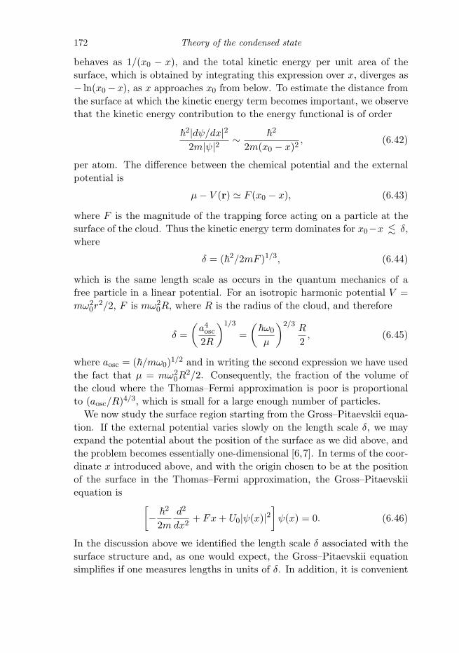
172 Theory of the condensed state
behaves as 1/(x0 − x), and the total kinetic energy per unit area of thesurface, which is obtained by integrating this expression over x, diverges as− ln(x0 −x), as x approaches x0 from below. To estimate the distance fromthe surface at which the kinetic energy term becomes important, we observethat the kinetic energy contribution to the energy functional is of order
�2|dψ/dx|22m|ψ|2 ∼ �
2
2m(x0 − x)2, (6.42)
per atom. The difference between the chemical potential and the externalpotential is
μ − V (r) � F (x0 − x), (6.43)
where F is the magnitude of the trapping force acting on a particle at thesurface of the cloud. Thus the kinetic energy term dominates for x0−x � δ,where
δ = (�2/2mF )1/3, (6.44)
which is the same length scale as occurs in the quantum mechanics of afree particle in a linear potential. For an isotropic harmonic potential V =mω2
0r2/2, F is mω2
0R, where R is the radius of the cloud, and therefore
δ =(
a4osc
2R
)1/3
=(
�ω0
μ
)2/3 R
2, (6.45)
where aosc = (�/mω0)1/2 and in writing the second expression we have usedthe fact that μ = mω2
0R2/2. Consequently, the fraction of the volume of
the cloud where the Thomas–Fermi approximation is poor is proportionalto (aosc/R)4/3, which is small for a large enough number of particles.
We now study the surface region starting from the Gross–Pitaevskii equa-tion. If the external potential varies slowly on the length scale δ, we mayexpand the potential about the position of the surface as we did above, andthe problem becomes essentially one-dimensional [6,7]. In terms of the coor-dinate x introduced above, and with the origin chosen to be at the positionof the surface in the Thomas–Fermi approximation, the Gross–Pitaevskiiequation is [
− �2
2m
d2
dx2+ Fx + U0|ψ(x)|2
]ψ(x) = 0. (6.46)
In the discussion above we identified the length scale δ associated with thesurface structure and, as one would expect, the Gross–Pitaevskii equationsimplifies if one measures lengths in units of δ. In addition, it is convenient

6.3 Surface structure of clouds 173
to measure the wave function of the condensate in terms of its value b =(Fδ/U0)1/2 in the Thomas–Fermi theory at a distance δ from the edge ofthe cloud. After introducing a scaled length variable y = x/δ and a scaledwave function given by Ψ = ψ/b we obtain the equation
Ψ′′ = yΨ + Ψ3, (6.47)
where a prime denotes differentiation with respect to y. The solution in theThomas–Fermi approximation is
Ψ =√−y for y ≤ 0, Ψ = 0 for y > 0. (6.48)
First let us consider the behaviour for x δ, corresponding to y 1.Since the condensate wave function is small we may neglect the cubic termin Eq. (6.47). The resulting equation is that for the Airy function, and itsasymptotic solution is
Ψ � C
y1/4e−2y3/2/3. (6.49)
Deep inside the cloud, corresponding to y −1, the Thomas–Fermi solu-tion Ψ � √−y is approximately valid. To determine the leading correctionto the wave function, we write Ψ = Ψ0 + Ψ1 and linearize (6.47), therebyfinding
−Ψ′′1 + yΨ1 + 3Ψ2
0Ψ1 = Ψ′′0. (6.50)
Using Ψ0 = (−y)1/2 from (6.48) and neglecting Ψ′′1 in (6.50) since it con-
tributes to terms of higher order in 1/y, we arrive at the result
Ψ1 � − 18y2
√−y. (6.51)
The asymptotic solution is thus
Ψ =√−y
(1 +
18y3
). (6.52)
Equation (6.47) may be solved numerically and this enables one to evaluatethe coefficient C in Eq. (6.49), which is found to be approximately 0.3971 [7].
We now evaluate the kinetic energy per unit area perpendicular to the x
axis,<p2>
2m=
�2
2m
∫dx|∇ψ|2. (6.53)
Let us first use the Thomas–Fermi wave function (6.48) which we expect tobe valid only in the region x −δ. Since the integral diverges for x → 0,as we discussed at the beginning of this section, we evaluate the integral for

174 Theory of the condensed state
x less than some cut-off value −l. We take the lower limit of the integrationto be −L, where L is large compared with δ. We expect that the kineticenergy will be given approximately by the Thomas–Fermi result if the cut-off distance is chosen to be ∼ −δ, the distance at which the Thomas–Fermiapproximation fails,
<p2>
2m=
�2
2m
∫ −l
−Ldx(ψ′)2 � �
2
8m
F
U0ln
L
l. (6.54)
We now compare this result with the kinetic energy per unit area calculatednumerically using the true wave function,
<p2>
2m=
�2
2m
∫ ∞
−Ldx(ψ′)2 ≈ �
2
8m
F
U0ln
4.160L
δ, (6.55)
which is valid for large values of ln(L/δ).We conclude that one obtains the correct asymptotic behaviour of the
kinetic energy if one uses the Thomas–Fermi approach and cuts the integraloff at x = −l, where
l = 0.240δ. (6.56)
As we shall demonstrate below, the same effective cut-off may be used forcalculating the kinetic energy in more general situations.
We now turn to the system of physical interest, a cloud of N atoms trappedin a three-dimensional harmonic-oscillator potential. For simplicity, we con-sider only the isotropic case, where the potential is V (r) = mω2
0r2/2. The
ground-state wave function satisfies the Gross–Pitaevskii equation[− �
2
2mr2
d
dr(r2 d
dr) +
12mω2
0r2 +
4π�2a
m|ψ(r)|2
]ψ(r) = μψ(r). (6.57)
By the substitution χ = rψ we obtain
− �2
2m
d2χ
dr2+
12mω2
0(r2 − R2)χ(r) +
4π�2a
mr2|χ(r)|2χ(r) = 0, (6.58)
since μ = mω20R
2/2. The Thomas–Fermi solution is
χTF = r
(R2 − r2
8πaa4osc
)1/2
. (6.59)
By expanding about r = R in Eq. (6.58) we arrive at an equation of theform (6.47), with the length scale δ given by Eq. (6.45).
To calculate the kinetic energy, we use the Thomas–Fermi wave function

6.4 Healing of the condensate wave function 175
and cut the integral off at a radius R− l, where l is given by the calculationfor the linear ramp, Eq. (6.56). The result is
Ekin
N=
�2
2m
∫ R−l0 drr2(dψ/dr)2∫ R
0 drr2ψ2� �
2
2mR2
(154
ln2R
l− 5
2
). (6.60)
This expression agrees well with the numerical result [7] for ln(R/δ) greaterthan 3, the relative difference being less than 2.5%.
6.4 Healing of the condensate wave function
In the previous section we considered the condensate wave function for anexternal potential that varied relatively smoothly in space. It is instructiveto investigate the opposite extreme, a condensate confined by a box withinfinitely hard walls. At the wall, the wave function must vanish, and in theinterior of the box the condensate density approaches its bulk value. Thedistance over which the wave function rises from zero at the wall to close toits bulk value may be estimated from the Gross–Pitaevskii equation, sinceaway from the wall the wave function is governed by competition betweenthe interaction energy term ∼ nU0 and the kinetic energy one. If one denotesthe spatial scale of variations by ξ, the kinetic energy per particle is of order�
2/2mξ2 and the two energies are equal when
�2
2mξ2= nU0, (6.61)
or
ξ2 =�
2
2mnU0=
18πna
=r3s
6a, (6.62)
where the particle separation rs is defined in Eq. (6.5). Since in experimentsthe distance between atoms is typically much larger than the scatteringlength, the coherence length is larger than the atomic separation. The lengthξ is referred to in the condensed matter literature as the coherence length,where the meaning of the word ‘coherence’ is different from that in optics.Since it describes the distance over which the wave function tends to its bulkvalue when subjected to a localized perturbation, it is also referred to as thehealing length.
To investigate the behaviour of the condensate wave function quantita-tively, we begin with the Gross–Pitaevskii equation (6.11), and assume thatthe potential vanishes for x ≥ 0 and is infinite for x < 0. The ground-state wave function is uniform in the y and z directions, and therefore the
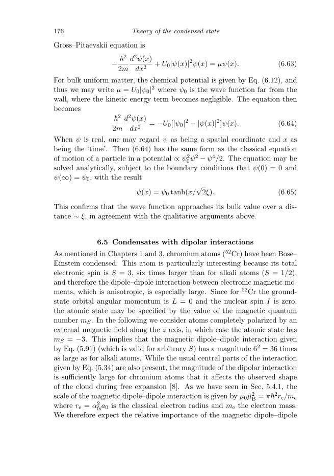
176 Theory of the condensed state
Gross–Pitaevskii equation is
− �2
2m
d2ψ(x)dx2
+ U0|ψ(x)|2ψ(x) = μψ(x). (6.63)
For bulk uniform matter, the chemical potential is given by Eq. (6.12), andthus we may write μ = U0|ψ0|2 where ψ0 is the wave function far from thewall, where the kinetic energy term becomes negligible. The equation thenbecomes
�2
2m
d2ψ(x)dx2
= −U0[|ψ0|2 − |ψ(x)|2]ψ(x). (6.64)
When ψ is real, one may regard ψ as being a spatial coordinate and x asbeing the ‘time’. Then (6.64) has the same form as the classical equationof motion of a particle in a potential ∝ ψ2
0ψ2 − ψ4/2. The equation may be
solved analytically, subject to the boundary conditions that ψ(0) = 0 andψ(∞) = ψ0, with the result
ψ(x) = ψ0 tanh(x/√
2ξ). (6.65)
This confirms that the wave function approaches its bulk value over a dis-tance ∼ ξ, in agreement with the qualitative arguments above.
6.5 Condensates with dipolar interactions
As mentioned in Chapters 1 and 3, chromium atoms (52Cr) have been Bose–Einstein condensed. This atom is particularly interesting because its totalelectronic spin is S = 3, six times larger than for alkali atoms (S = 1/2),and therefore the dipole–dipole interaction between electronic magnetic mo-ments, which is anisotropic, is especially large. Since for 52Cr the ground-state orbital angular momentum is L = 0 and the nuclear spin I is zero,the atomic state may be specified by the value of the magnetic quantumnumber mS . In the following we consider atoms completely polarized by anexternal magnetic field along the z axis, in which case the atomic state hasmS = −3. This implies that the magnetic dipole–dipole interaction givenby Eq. (5.91) (which is valid for arbitrary S) has a magnitude 62 = 36 timesas large as for alkali atoms. While the usual central parts of the interactiongiven by Eq. (5.34) are also present, the magnitude of the dipolar interactionis sufficiently large for chromium atoms that it affects the observed shapeof the cloud during free expansion [8]. As we have seen in Sec. 5.4.1, thescale of the magnetic dipole–dipole interaction is given by μ0μ
2B = π�
2re/me
where re = α2fsa0 is the classical electron radius and me the electron mass.
We therefore expect the relative importance of the magnetic dipole–dipole

6.5 Condensates with dipolar interactions 177
interaction compared with the central interaction to be governed by thedimensionless parameter α2
fs(m/me)(a0/a), as will be confirmed by the de-tailed calculation below.
As an illustration, we calculate within the Thomas–Fermi approximationthe deformation of a trapped cloud due to the dipolar interaction [9]. Thedipolar interaction energy between two atoms at points r and r′ is givenaccording to Eq. (5.91) by
Umd(r − r′) =μ0(2mSμB)2
4π
(1
|r − r′|3 − 3(z − z′)2
|r − r′|5)
. (6.66)
This interaction is long-ranged. The energy due to it may be calculated inthe mean-field approximation, and it is given for the wave function (6.1) by
Emd =12
∫drdr′Umd(r − r′)n(r)n(r′), (6.67)
where n(r) is given by Eq. (6.8).6 The equation for the condensate wavefunction may be determined by repeating the considerations in Sec. 6.1 withthe dipolar contribution to the energy included and one finds the Gross–Pitaevskii equation
− �2
2m∇2ψ(r) + V (r)ψ(r) +
[U0|ψ(r)|2 +
∫dr′Umd(r − r′)|ψ(r′)|2
]ψ(r)
= μψ(r). (6.68)
In the Thomas–Fermi approximation, the density distribution n(r) satisfiesthe integral equation
μ = V (r) + U0n(r) +∫
dr′Umd(r − r′)n(r′), (6.69)
which is a generalization of Eq. (6.31) in the absence of the dipolar inter-action. For simplicity we consider in the following an isotropic harmonictrap with V (r) = mω2
0r2/2 and treat the dipolar interaction as a perturba-
tion. In the absence of the dipolar interaction, Eq. (6.69) has the solutionn(0)(r) = (μ − mω2
0r2/2)/U0. We insert this n(0)(r) into the last term of
(6.69) and carry out the integration over r′ and obtain the dipolar contri-
6 Equation (6.67) contains the bare dipole–dipole interaction. This is because the dipolar in-teraction is long-ranged but is small for a given pair of atoms, and therefore correlations areunimportant. This situation is to be contrasted with that of the central interactions, for whichthe effective interaction is different from bare interaction. The mean-field theory appropriatefor the dipolar interaction is the usual one known from plasma physics, not one similar toLandau Fermi-liquid theory that we used in treating the central part of the interaction.

178 Theory of the condensed state
bution to the energy of an atom at point r:
V(0)md (r) =
∫dr′Umd(r − r′)n(0)(r′). (6.70)
From Eq. (6.69) one then finds
n(r) =1U0
[μ − V (r) − V(0)md (r)]. (6.71)
As we shall see, V(0)md (r) is anisotropic and as a consequence the cloud is
distorted. The integrand in (6.69) may be simplified by using the relation
1|r − r′|3 − 3(z − z′)2
|r − r′|5 = − ∂2
∂z2
(1
|r − r′|
)− 4π
3δ(r − r′). (6.72)
Inserting this result into Eq. (6.70) one finds
V(0)md (r) = −μ0(2mSμB)2
(∂2φ(r)
∂z2+
13n(0)(r)
), (6.73)
where
φ(r) =14π
∫dr′
n(0)(r′)|r− r′| . (6.74)
Thus φ satisfies the Poisson equation ∇2φ = −n(0)(r) and is, apart fromfactors, the electrostatic potential due to a charge distribution n(0)(r).
In the case we consider, n(0) is spherically symmetric and given by n(0) =n(0)(0)(1−r2/R2) for r less than the Thomas–Fermi radius R. The potentialat r is determined by splitting up the integration in (6.74) into two regions,r′ < r and r′ > r. The contribution of the former region is given by 1/r timesthe total number of atoms inside the sphere with radius r. The contributionto the potential from a spherical shell with radius r′ > r and thickness dr′ is1/r′ times the total charge contained in the shell, and therefore the potentialis
φ(r) =1r
∫ r
0dr′(r′)2n(0)(r′) +
∫ R
rdr′(r′)2
1r′
n(0)(r′), (6.75)
or
φ(r) = n(0)(0)(
R2
4− r2
6+
r4
20R2
), (6.76)
for r < R and φ = N/4πr for r > R. The energy V(0)md (r) given by the last

6.5 Condensates with dipolar interactions 179
term in (6.69) is thus
V(0)md (r) =
∫dr′Umd(r− r′)n(0)(r′) = −μ0(2mSμB)2
(∂2
∂z2φ(r) +
13n(0)(r)
).
(6.77)When (6.76) is inserted into this expression one gets
V(0)md (r) =
215
μ0(2mSμB)2n(0)(0)(
r2 − 3z2
R2
)
=mω2
0
15U0μ0(2mSμB)2(x2 + y2 − 2z2), (6.78)
where the second form follows from the fact that in the Thomas–Fermiapproximation n(0)(0) = mω2
0R2/2U0. From Eq. (6.71) one thus finds
n(r) = n(0)(0)(
1 − x2
R2x
− y2
R2y
− z2
R2z
)(6.79)
where
Rx = Ry � R(1 − εdd/5); Rz � R(1 + 2εdd/5) (6.80)
to lowest order in the dimensionless parameter
εdd =μ0(2mSμB)2m
12π�2a=
m2S
3πα2
fs
(m
me
)(a0
a
). (6.81)
For 52Cr in the mS = −3 state and for the measured scattering lengtha = 100a0, the value of εdd is 0.15 [10].
The dipolar interaction thus elongates the cloud along the direction inwhich the dipoles are aligned. The physical reason is that the interaction isattractive when the relative separation points along the z axis and repulsivewhen it lies in the plane perpendicular to it. The perturbation treatmentmay be extended to anisotropic traps.
The experiment of Ref. [8] was carried out with a chromium condensatein an anisotropic harmonic trap with three different trap frequencies. Theatomic dipole moments were oriented by a homogeneous magnetic field, andthe aspect ratio Ry/Rz during expansion was measured as a function oftime for two different directions of the magnetic field, thus allowing thesmall effects of the magnetic dipole–dipole interaction to be identified.
Problems
Problem 6.1 Consider N bosons interacting via repulsive interactionsin an isotropic harmonic trap. Use the Gaussian trial function (6.18) to

180 Theory of the condensed state
calculate the kinetic energy per particle of a cloud in its ground state whenNa/aosc is large.
Problem 6.2 Consider a condensate which is trapped by a potential whichis a homogeneous function of degree ν of the radial coordinate but with arbi-trary dependence on the angular coordinates (V (λr) = λνV (r)). In equilib-rium, the energy of the condensate must be unchanged by a small change inthe wave function from its value in the ground state, subject to the numberof particles being constant. By considering a change of spatial scale of thewave function, with its form being unaltered, show that the kinetic, trapand interaction energies, which are given by Ekin = (�2/2m)
∫dr|∇ψ(r)|2,
Etrap =∫
drV (r)|ψ(r)|2, and Eint = 12U0
∫dr|ψ(r)|4 satisfy the condition
2Ekin − νEtrap + 3Eint = 0,
which is a statement of the virial theorem for this problem. Show in additionthat the chemical potential is given by
μN = Ekin + Etrap + 2Eint,
and determine the ratio between the chemical potential and the total energyper particle in the limit when the kinetic energy may be neglected.
Problem 6.3 Consider a cloud of 105 atoms of 87Rb in an isotropicharmonic-oscillator potential with the oscillation frequency ω0 given byω0/2π = 200 Hz. Calculate the total energy, the chemical potential μ, theradius R, in the Thomas–Fermi approximation, taking the scattering lengtha to be 100a0. Use these results to estimate the coherence length ξ at thecentre of the cloud, and the length δ giving the scale of surface structure.
References[1] L. P. Pitaevskii, Zh. Eksp. Teor. Fiz. 40, 646 (1961) [Sov. Phys.–JETP 13,
451 (1961)]; E. P. Gross, Nuovo Cimento 20, 454 (1961); J. Math. Phys. 4,195 (1963).
[2] Our discussion is based on that of G. Baym and C. J. Pethick, Phys. Rev.Lett. 76, 6 (1996). Some of the results were obtained earlier by R. V. E.Lovelace and T. J. Tommila, Phys. Rev. A 35, 3597 (1987).
[3] C. C. Bradley, C. A. Sackett, J. J. Tollett, and R. G. Hulet, Phys. Rev. Lett.75, 1687 (1995); C. C. Bradley, C. A. Sackett, and R. G. Hulet, Phys. Rev.Lett. 78, 985 (1997).
[4] A. L. Fetter, cond-mat/9510037.[5] P. A. Ruprecht, M. J. Holland, K. Burnett, and M. Edwards, Phys. Rev. A
51, 4704 (1995).[6] F. Dalfovo, L. P. Pitaevskii, and S. Stringari, Phys. Rev. A 54, 4213 (1996).

References 181
[7] E. Lundh, C. J. Pethick, and H. Smith, Phys. Rev. A 55, 2126 (1997).[8] J. Stuhler, A. Griesmaier, T. Koch, M. Fattori, T. Pfau, S. Giovanazzi, P.
Pedri, and L. Santos, Phys. Rev. Lett. 95, 150406 (2005).[9] S. Giovanazzi, A. Gorlitz, and T. Pfau, Phys. Rev. Lett. 89, 130401 (2002).
[10] J. Werner, A. Griesmaier, S. Hensler, J. Stuhler, T. Pfau, A. Simoni, and E.Tiesinga, Phys. Rev. Lett. 94, 183201 (2005).

7
Dynamics of the condensate
The time-dependent behaviour of Bose–Einstein condensed clouds, such ascollective modes and the expansion of a cloud when released from a trap, isan important source of information about the physical nature of the conden-sate. In addition, the spectrum of elementary excitations of the condensateis an essential ingredient in calculations of thermodynamic properties. Inthis chapter we treat the dynamics of a condensate at zero temperaturestarting from a time-dependent generalization of the Gross–Pitaevskii equa-tion used in Chapter 6 to describe static properties. From this equationone may derive equations very similar to those of classical hydrodynamics,which we shall use to calculate properties of collective modes.
We begin in Sec. 7.1 by describing the time-dependent Gross–Pitaevskiiequation and deriving the hydrodynamic equations, which we then use todetermine the excitation spectrum of a homogeneous Bose gas (Sec. 7.2).Subsequently, we consider modes in trapped clouds (Sec. 7.3) within thehydrodynamic approach, and also describe the method of collective coordi-nates and the related variational method. In Sec. 7.4 we consider surfacemodes of oscillation, which resemble gravity waves on a liquid surface. Thevariational approach is used in Sec. 7.5 to treat the free expansion of a con-densate upon release from a trap. Finally, in Sec. 7.6 we discuss solitons,which are exact one-dimensional non-linear solutions of the time-dependentGross–Pitaevskii equation.
7.1 General formulation
In the previous chapter we saw that the equilibrium structure of the conden-sate is described by a time-independent Schrodinger equation with a non-linear contribution to the potential to take into account interactions betweenparticles. To treat dynamical problems it is natural to use a time-dependent
182

7.1 General formulation 183
generalization of this Schrodinger equation, with the same non-linear inter-action term. This equation is the time-dependent Gross–Pitaevskii equation,
i�∂ψ(r, t)
∂t= − �
2
2m∇2ψ(r, t) + V (r)ψ(r, t) + U0|ψ(r, t)|2ψ(r, t), (7.1)
which is the basis for our discussion of the dynamics of the condensate.The time-independent Gross–Pitaevskii equation, Eq. (6.11), is a non-
linear Schrodinger equation with the chemical potential replacing the en-ergy eigenvalue in the time-independent Schrodinger equation. To ensureconsistency between the time-dependent Gross–Pitaevskii equation and thetime-independent one, under stationary conditions ψ(r, t) must develop intime as exp(−iμt/�). The phase factor reflects the fact that microscopicallyψ is equal to the matrix element of the annihilation operator ψ between theground state with N particles and that with N − 1 particles,
ψ(r, t) = 〈N − 1|ψ(r)|N〉 ∝ exp[−i(EN − EN−1)t/�], (7.2)
since the states |N〉 and |N − 1〉 develop in time as exp(−iEN t/�) andexp(−iEN−1t/�), respectively. For large N the difference in ground-stateenergies EN−EN−1 is equal to ∂E/∂N , which is the chemical potential.Therefore this result is basically the Josephson relation for the developmentof the phase φ of the condensate wave function
dφ
dt= −μ
�. (7.3)
Both for formal reasons as well as for applications a variational formu-lation analogous to that for static problems is useful. The time-dependentGross–Pitaevskii equation (7.1) may be derived from the action principle
δ
∫ t2
t1
Ldt = 0, (7.4)
where the Lagrangian L is given by
L =∫
dri�
2
(ψ∗∂ψ
∂t− ψ
∂ψ∗
∂t
)− E
=∫
dr[i�
2
(ψ∗∂ψ
∂t− ψ
∂ψ∗
∂t
)− E]. (7.5)
Here E is the energy, Eq. (6.9), and the energy density E is given by
E =�
2
2m|∇ψ|2 + V (r)|ψ|2 +
U0
2|ψ|4. (7.6)
In the variational principle (7.4) the variations of ψ (or ψ∗) are arbitrary,
184 Dynamics of the condensate
apart from the requirement that they vanish at t = t1, t = t2, and onany spatial boundaries for all t. With a physically motivated choice oftrial function for ψ, this variational principle provides the foundation forapproximate solutions of dynamical problems, as we shall illustrate in Sec.7.3.3.
The physical content of the Gross–Pitaevskii equation (7.1) may be re-vealed by reformulating it as a pair of hydrodynamic equations, which wenow derive.
7.1.1 The hydrodynamic equations
Under general, time-dependent conditions we may use instead of (7.1) anequivalent set of equations for the density, which is given by |ψ|2, and thegradient of its phase, which is proportional to the local velocity of the con-densate.
To understand the nature of the velocity of the condensate, we derive thecontinuity equation. If one multiplies the time-dependent Gross–Pitaevskiiequation (7.1) by ψ∗(r, t) and subtracts the complex conjugate of the result-ing equation, one arrives at the equation
∂|ψ|2∂t
+ ∇ ·[
�
2mi(ψ∗∇ψ − ψ∇ψ∗)
]= 0. (7.7)
This is the same as one obtains from the usual (linear) Schrodinger equa-tion, since the non-linear potential in the Gross–Pitaevskii equation is real.Equation (7.7) has the form of a continuity equation for the particle density,n = |ψ|2, and it may be written as
∂n
∂t+ ∇ · (nv) = 0, (7.8)
where the velocity of the condensate is defined by
v =�
2mi
(ψ∗∇ψ − ψ∇ψ∗)|ψ|2 . (7.9)
The momentum density j is given by
j =�
2i(ψ∗∇ψ − ψ∇ψ∗), (7.10)
and therefore the relation (7.9) is equivalent to the result
j = mnv, (7.11)
which states that the momentum density is equal to the particle mass timesthe particle current density.

7.1 General formulation 185
Simple expressions for the density and velocity may be obtained if wewrite ψ in terms of its amplitude f and phase φ,
ψ = feiφ, (7.12)
from which it follows that
n = f2, (7.13)
and the velocity v is
v =�
m∇φ. (7.14)
From Eq. (7.14) we conclude that the motion of the condensate correspondsto potential flow, since the velocity is the gradient of a scalar quantity,which is referred to as the velocity potential. For a condensate, Eq. (7.14)shows that the velocity potential is �φ/m. Provided that φ is not singular,we can immediately conclude that the motion of the condensate must beirrotational, that is1
∇×v =�
m∇×∇φ = 0. (7.15)
The possible motions of a condensate are thus much more restricted thanthose of a classical fluid.
The equations of motion for f and φ may be found by inserting (7.12)into (7.1) and separating real and imaginary parts. Since
i∂ψ
∂t= i
∂f
∂teiφ − ∂φ
∂tfeiφ (7.16)
and
−∇2ψ = [−∇2f + (∇φ)2f − i(∇2φ)f − 2i(∇φ) · ∇f ]eiφ, (7.17)
we obtain the two equations
∂(f2)∂t
= − �
m∇ · (f2∇φ) (7.18)
and
−�∂φ
∂t= − �
2
2mf∇2f +
12mv2 + V (r) + U0f
2. (7.19)
Equations (7.18) and (7.19) may also be derived directly from the variationalprinciple (7.4) with the Lagrangian (7.5) expressed in terms of the variablesn = f2 and φ, and this is left as an exercise (Problem 7.1).1 Note that this result applies only if φ is not singular. This condition is satisfied in the examples
we consider in this chapter, but it fails at, e.g., the core of a vortex line. The properties ofvortices will be treated in Chapter 9.

186 Dynamics of the condensate
Equation (7.18) is the continuity equation (7.8) expressed in the newvariables. To find the equation of motion for the velocity, given by Eq.(7.14), we take the gradient of Eq. (7.19), and the resulting equation is
m∂v∂t
= −∇(μ +12mv2), (7.20)
where
μ = V + nU0 −�
2
2m√
n∇2√n. (7.21)
Equation (7.19) may be expressed in terms of the functional derivative2
δE/δn,
∂φ(r, t)∂t
= −1�
δE
δn(r). (7.22)
The quantity δE/δn(r) is the energy required to add a particle at point r,and therefore this result is the generalization of the Josephson relation (7.3)to systems not in their ground states. Under stationary conditions μ+ 1
2mv2
is a constant, and if in addition the velocity is zero, that is φ is independentof position, μ is a constant, which is precisely the time-independent Gross–Pitaevskii equation (6.11).
The quantity nU0 in Eq. (7.21) is the expression for the chemical potentialof a uniform Bose gas, omitting contributions from the external potential.At zero temperature, changes in the chemical potential for a bulk system arerelated to changes in the pressure p by the Gibbs–Duhem relation dp = ndμ,a result easily confirmed for the uniform dilute Bose gas, since μ = nU0 andp = −∂E/∂V = n2U0/2 (see Eqs. (6.12) and (6.6), respectively). Equation(7.20) may therefore be rewritten in the form
∂v∂t
= − 1mn
∇p − ∇(
v2
2
)+
1m
∇(
�2
2m√
n∇2√n
)− 1
m∇V. (7.23)
Equations (7.8) and (7.23) are very similar to the hydrodynamic equationsfor an ideal fluid. If we denote the velocity of the fluid by v, the continuityequation (7.8) has precisely the same form as for an ideal fluid, while the
2 The functional derivative δE/δn(r) of the energy is defined according to the equation δE =∫dr[δE/δn(r)]δn(r), and it is a function of r with the dimension of energy. It is given in terms
of the energy density (7.6), which is a function of n and ∇n, by
δE
δn(r)=
∂E∂n
−∑
i
∂
∂xi
∂E∂(∂n/∂xi)
,
where the sum is over the three spatial coordinates.
7.1 General formulation 187
analogue of Eq. (7.23) is the Euler equation
∂v∂t
+ (v · ∇)v +1
mn∇p = − 1
m∇V, (7.24)
or∂v∂t
− v × (∇ × v) = − 1mn
∇p − ∇(
v2
2
)− 1
m∇V. (7.25)
Here the pressure p is that of the fluid, which generally has a form differentfrom that of the condensate.
There are two differences between equations (7.23) and (7.25). The firstis that the Euler equation contains the term v×(∇×v). However, since thevelocity field of the superfluid corresponds to potential flow, ∇×v = 0, theterm v × (∇ × v) for such a flow would not contribute in the Euler equation.The only difference between the two equations for potential flow is thereforethe third term on the right-hand side of Eq. (7.23), which is referred to asthe quantum pressure term. This describes forces due to spatial variationsin the magnitude of the wave function for the condensed state. Like theterm ∇v2/2, its origin is the kinetic energy term �
2|∇ψ|2/2m = mnv2/2 +�
2(∇f)2/2m in the energy density, but the two contributions correspond todifferent physical effects: the first is the kinetic energy of motion of particles,while the latter corresponds to ‘zero-point motion’, which does not give riseto particle currents. If the spatial scale of variations of the condensate wavefunction is l, the pressure term in Eq. (7.23) is of order nU0/ml, while thequantum pressure term is of order �
2/m2l3. Thus the quantum pressure termdominates the usual pressure term if spatial variations of the density occuron length scales l less than or of order the coherence length ξ ∼ �/(mnU0)1/2
(see Eq. (6.62)), and it becomes less important on larger length scales.As we have seen, motions of the condensate may be specified in terms
of a local density and a local velocity. The reason for this is that the onlydegrees of freedom are those of the condensate wave function, which hasa magnitude and a phase. Ordinary liquids and gases have many moredegrees of freedom and, as a consequence, it is in general necessary to em-ploy a microscopic description, e.g., in terms of the distribution function forthe particles. However, a hydrodynamic description is possible for ordinarygases and liquids if collisions between particles are sufficiently frequent thatthermodynamic equilibrium is established locally. The state of the fluid maythen be specified completely in terms of the local particle density (or equiv-alently the mass density), the local velocity, and the local temperature. Atzero temperature, the temperature is not a relevant variable, and the motionmay be described in terms of the local density and the local fluid velocity,

188 Dynamics of the condensate
just as for a condensate. The reason that the equations of motion for acondensate and for a perfect fluid are so similar is that they are expressionsof the conservation laws for particle number and for total momentum. How-ever, the physical reasons for a description in terms of a local density and alocal velocity being possible are quite different for the two situations.
7.2 Elementary excitations
The properties of elementary excitations may be investigated by consideringsmall deviations of the state of the gas from equilibrium and finding periodicsolutions of the time-dependent Gross–Pitaevskii equation. An equivalentapproach is to use the hydrodynamic formulation given above, and we beginby describing this. In Chapter 8 we shall consider the problem on the basisof microscopic theory. We write the density as n = neq+δn, where neq is theequilibrium density and δn the departure of the density from its equilibriumvalue. On linearizing Eqs. (7.8), (7.20), and (7.21) by treating the velocityv and δn as small quantities, one finds
∂δn
∂t= −∇ · (neqv) (7.26)
and
m∂v∂t
= −∇δμ, (7.27)
where δμ is obtained by linearizing (7.21). Taking the time derivative of(7.26) and eliminating the velocity by means of (7.27) results in the equationof motion
m∂2δn
∂t2= ∇ · (neq∇δμ). (7.28)
This equation describes the excitations of a Bose gas in an arbitrary po-tential. To keep the notation simple, we shall henceforth in this chapterdenote the equilibrium density by n. Note that n is the density of the con-densate, since we neglect the zero-temperature depletion of the condensate.In Chapter 10, which treats the dynamics at non-zero temperature, we shalldenote the condensate density by n0, in order to distinguish it from the totaldensity, which includes a contribution from thermal excitations.
A uniform gas
As a first example we investigate the spectrum for a homogeneous gas,where the external potential V is constant. In the undisturbed state the

7.2 Elementary excitations 189
density n is the same everywhere and it may therefore be taken outsidethe spatial derivatives. We look for travelling-wave solutions, proportionalto exp(iq · r − iωt), where q is the wave vector and ω the frequency. FromEq. (7.21) the change in μ is seen to be equal to
δμ =(
U0 +�
2q2
4mn
)δn (7.29)
and the equation of motion becomes
mω2δn =(
nU0q2 +
�2q4
4m
)δn. (7.30)
To make contact with the microscopic calculations to be described later,it is convenient to work with the energy of an excitation, εq, rather thanthe frequency. Non-vanishing solutions of (7.30) are possible only if thefrequency is given by
�ω = ±εq, where εq =√
2nU0ε0q + (ε0q)2. (7.31)
Here
ε0q =�
2q2
2m(7.32)
is the free-particle energy (we adopt the convention that the branch of thesquare root to be used is the positive one). The spectrum (7.31) was firstderived by Bogoliubov from microscopic theory [1].
The excitation spectrum �ω = εq is plotted in Fig. 7.1. For small q, εq isa linear function of q,
εq � s�q, (7.33)
and the spectrum is sound-like. The velocity s is seen to be
s =√
nU0/m. (7.34)
This result agrees with the expression for the sound velocity calculated fromthe hydrodynamic result s2 = dp/dρ = (n/m)dμ/dn, where ρ = nm is themass density. The repulsive interaction has thus turned the energy spec-trum at long wavelengths, which is quadratic in q for free particles, intoa linear one, in agreement with what is observed experimentally in liquid4He. As we shall see in Chapter 10, the linear spectrum at long wavelengthsprovides the key to superfluid behaviour, and it was one of the triumphsof Bogoliubov’s pioneering calculation. In the hydrodynamic description

190 Dynamics of the condensate
Fig. 7.1 Excitation spectrum of a homogeneous Bose gas (full line) plotted as afunction of the wave number expressed as the dimensionless variable �q/ms, wherethe sound velocity s is given by Eq. (7.34). The expansion (7.35) for high wavenumber is shown as a dotted line.
the result is almost ‘obvious’, since sound waves are well-established excita-tions of hydrodynamic systems. What is perhaps surprising is that at shortwavelengths the leading contributions to the spectrum are
εq � ε0q + nU0, (7.35)
which is also shown in Fig. 7.1. This is the free-particle spectrum plus amean-field contribution. The transition between the linear spectrum and thequadratic one occurs when the kinetic energy, �
2q2/2m, becomes comparablewith the potential energy of a particle ∼ nU0, or in other words the ‘quantumpressure’ term and the usual pressure term are roughly equal. This occursat a wave number ∼ (2mnU0)1/2/�, which is the inverse of the coherencelength, ξ, Eq. (6.62). The coherence length is related to the sound velocity,Eq. (7.34) by ξ = �/
√2ms. On length scales longer than ξ, atoms move
collectively, while on shorter length scales, they behave as free particles.The spectrum of elementary excitations in superfluid liquid 4He differs fromthat for a dilute gas because of the strong short-range correlations. Thefirst satisfactory account of the roton part of the spectrum was given byFeynman [2].
The energy of the elementary excitations can also be obtained by calculat-ing the response of the condensate to a space- and time-dependent external

7.2 Elementary excitations 191
potential V (r, t) = Vq exp(iq · r− iωt). To see this one adds the term −∇V
on the right-hand side of Eq. (7.28), which results in
m
(ω2 −
ε2q�2
)δn = nq2Vq, (7.36)
or
δn = χ(q, ω)Vq, (7.37)
where
χ(q, ω) =nq2
m(ω2 − ε2q/�2)(7.38)
is the density–density response function for the condensate. Thus the re-sponse diverges if the frequency of the external potential is equal to thefrequency of an elementary excitation of the condensate. In Chapter 16 weshall use the expression for the response function to calculate how the inter-action between two fermions is affected by the presence of a condensate ofbosons. Response functions are of general importance in many experimentalsituations, since external probes such as electromagnetic waves or neutronsusually couple weakly to the system of interest, implying that the responseof the system will be determined by its elementary excitations.
The Bogoliubov equations
An alternative route to calculating the excitation spectrum is to start fromthe Gross–Pitaevskii equation directly, without introducing the hydrody-namic variables. This approach complements the hydrodynamic one sinceit emphasizes single-particle behaviour and shows how the collective effectsat long wavelengths come about. Let us denote the change in ψ by δψ.Linearizing the Gross–Pitaevskii equation (7.1), one finds
− �2
2m∇2δψ(r, t) + V (r)δψ(r, t)+ U0[2|ψ(r, t)|2δψ(r, t) + ψ(r, t)2δψ∗(r, t)]
= i�∂δψ(r, t)
∂t(7.39)
and
− �2
2m∇2δψ∗(r, t) + V (r)δψ∗(r, t) + U0[2|ψ(r, t)|2δψ∗(r, t) + ψ∗(r, t)2δψ(r, t)]
= −i�∂δψ∗(r, t)
∂t. (7.40)

192 Dynamics of the condensate
Here ψ(r, t) is understood to be the condensate wave function in the un-perturbed state, which we may write as ψ =
√n(r)e−iμt/�, where n(r) is
the equilibrium density of particles and μ is the chemical potential of theunperturbed system. To avoid carrying an arbitrary phase factor along inour calculations we have taken the phase of the condensate wave functionat t = 0 to be zero. We wish to find solutions of these equations which areperiodic in time, apart from the overall phase factor e−iμt/� present for theunperturbed state. We therefore search for solutions of the form
δψ(r, t) = e−iμt/�[u(r)e−iωt − v∗(r)eiωt
], (7.41)
where u(r) and v(r) are functions to be determined and ω is real. Theoverall phase factor e−iμt/� is necessary to cancel the effects of the phasesof ψ(r, t)2 and ψ∗(r, t)2 in Eqs. (7.39) and (7.40), and thereby ensure thatthe equations can be satisfied for all time. The choice of the sign in frontof v is a matter of convention, and we take it to be negative. Since theequations couple δψ and δψ∗, they cannot be satisfied unless both positiveand negative frequency components are allowed for. We insert the ansatz(7.41) into the two equations (7.39) and (7.40) and, provided ω �= 0, we mayequate to zero the coefficients of eiωt and e−iωt. This gives the following pairof coupled equations for u(r) and v(r):[
− �2
2m∇2 + V (r) + 2n(r)U0 − μ − �ω
]u(r) − n(r)U0v(r) = 0 (7.42)
and[− �
2
2m∇2 + V (r) + 2n(r)U0 − μ + �ω
]v(r) − n(r)U0u(r) = 0, (7.43)
which are referred to as the Bogoliubov equations.We now apply this formalism to the uniform Bose gas, V (r) = 0. Because
of the translational invariance the solutions may be chosen to be of the form
u(r) = uqeiq·r
V 1/2and v(r) = vq
eiq·r
V 1/2, (7.44)
where we have introduced the conventional normalization factor 1/V 1/2 ex-plicitly, V being the volume of the system.
The chemical potential for the uniform system is given by nU0 (Eq. (6.12)),and thus the Bogoliubov equations are(
�2q2
2m+ nU0 − �ω
)uq − nU0vq = 0 (7.45)

7.2 Elementary excitations 193
and (�
2q2
2m+ nU0 + �ω
)vq − nU0uq = 0. (7.46)
The two equations are consistent only if the determinant of the coefficientsvanishes. With the definition (7.32) this leads to the condition
(ε0q + nU0 + �ω)(ε0q + nU0 − �ω) − n2U20 = 0, (7.47)
or
(�ω)2 = (ε0q + nU0)2 − (nU0)2 = ε0q(ε0q + 2nU0) = ε2q , (7.48)
which agrees with the spectrum (7.31) obtained earlier from the hydrody-namic approach.
The nature of the excitations may be elucidated by investigating the be-haviour of the coefficients uq and vq. Here we shall consider repulsive in-teractions, in which case the frequencies are real. For the positive energysolutions (�ω = +εq), one has
vq =nU0
εq + ξquq, (7.49)
where
ξq = ε0q + nU0 (7.50)
is the energy of an excitation if one neglects coupling between uq and vq.The normalization of uq and vq is arbitrary, but as we shall see from thequantum-mechanical treatment in Sec. 8.1, a convenient one is
|uq|2 − |vq|2 = 1, (7.51)
since this ensures that the new operators introduced there satisfy Bose com-mutation relations. The Bogoliubov equations are unaltered if uq and vq aremultiplied by an arbitrary phase factor. Therefore, without loss of generalitywe may take uq and vq to be real. With this choice one finds that
u2q =
12
(ξq
εq+ 1)
(7.52)
and
v2q =
12
(ξq
εq− 1)
. (7.53)
In terms of ξq, the excitation energy is given by
εq =√
ξ2q − (nU0)2. (7.54)

194 Dynamics of the condensate
Fig. 7.2 The coefficients uq and vq given by Eqs. (7.52)–(7.53) as functions of thewave number, expressed as the dimensionless variable �q/ms.
The coefficients uq and vq are exhibited as functions of the dimensionlessvariable �q/ms in Fig. 7.2.
For the positive energy solution, vq tends to zero as 1/q2 for large q,and in this limit δψ = ei(q·r−ωqt)/V 1/2, with ωq = εq/�. This correspondsto addition of a single particle with momentum �q, and the removal ofa particle in the zero-momentum state, as will be made explicit when thequantum-mechanical theory is presented in Chapter 8. At smaller momenta,excitations are linear superpositions of the state in which a particle with mo-mentum �q is added (and a particle in the condensate is removed) and thestate in which a particle with momentum −�q is removed (and a particleadded to the condensate). At long wavelengths uq and vq diverge as 1/q1/2,and the two components of the wave function are essentially equal in mag-nitude. For the negative energy solution (�ω = −εq) one has v2
q ≥ u2q and
uq → 0 for large q. In the large-q limit the excitation corresponds to theremoval of a particle with momentum −�q (and addition of a particle to thecondensate).
The algebraic expressions for the excitation spectrum and the factors uq
and vq are analogous to those for a superconductor in the Bardeen–Cooper–Schrieffer (BCS) theory, apart from some sign changes due to the fact thatwe are here dealing with bosons rather than fermions. In the BCS theory,

7.2 Elementary excitations 195
which we shall describe in Sec. 16.3 in the context of the transition to asuperfluid state for dilute Fermi gases, the dispersion relation for an ele-mentary excitation is εq =
√ξ2q + Δ2, where ξq is the normal-state energy of
a particle measured with respect to the chemical potential, as for the bosonproblem we consider, and Δ is the superconducting energy gap. Thus onesees that for bosons the excitation energy is obtained by replacing Δ2 in theBCS expression by −(nU0)2.
In addition to the finite-wavelength modes discussed above, there are twospecial modes. One corresponds to an overall change of the phase of thewave function, ψ → ψeiθ, where θ is real. For small θ the change in thewave function is δψ � iθψ. This does not change the energy, and thereforethere is no restoring force on this mode. The second mode corresponds toa uniform change in the magnitude of the condensate wave function. Ifthe change in the number of particles is ΔN , the condensate wave functionbehaves as
ψ =(
N + ΔN
V
)1/2
eiφ0e−iμ(N+ΔN)t/�, (7.55)
where μ(N + ΔN) is the chemical potential for particle number N + ΔN
and φ0 is the initial phase. This mode does not have the form assumed inthe ansatz (7.41). Uniform changes in the phase and density of particles areuncoupled, in contrast to the situation at finite wavelength, for which aninitial density fluctuation will, with time, give rise to a phase fluctuation.For a non-uniform condensate these modes will be discussed in greater detailin Sec. 8.2.
Attractive interactions
If the interaction is attractive, the sound speed is imaginary, which indicatesthat long-wavelength modes grow or decay exponentially in time, ratherthan oscillate. This signals an instability of the system due to the attractiveinteraction tending to make atoms clump together. However at shorterwavelengths modes are stable, since the free-particle kinetic energy termdominates in the dispersion relation. The lowest wave number qc for whichthe mode is stable is given by the condition that its frequency vanish. Thusfrom Eq. (7.31)
ε0qc+ 2nU0 = 0 (7.56)
or
q2c = −4mnU0
�2= 16πn|a|, (7.57)

196 Dynamics of the condensate
where we have used Eq. (5.33) to express U0 in terms of the scatteringlength a. This shows that the spatial scale of unstable modes is greater thanor of order the coherence length, Eq. (6.62), evaluated using the absolutemagnitude of the scattering length.
It is instructive to relate these ideas for bulk matter to a cloud in a trap.For simplicity, we consider the trap to be a spherical container with radiusR0. The lowest mode has a wave number of order 1/R0, and the density isn ∼ N/R3
0. Thus according to (7.57) the lowest mode is stable if the numberof particles is less than a critical value Nc given by 1/R2
0 ∼ Nc|a|/R30 or
Nc ∼R0
|a| , (7.58)
and unstable for larger numbers of particles. The physics of the instabilityis precisely the same as that considered in Chapter 6 in connection with theenergy of a cloud: for a sufficiently large number of particles, the zero-pointenergy of atoms is too small to overcome the attraction between them. In thepresent formulation, the zero-point energy is the kinetic energy of the lowestmode in the well. To make contact with the calculations for a harmonic-oscillator trap in Chapter 6, we note that the estimate (7.58) is consistentwith the earlier result (6.29) if the radius R0 of the container is replaced bythe oscillator length.
7.3 Collective modes in traps
Calculating the properties of modes in a homogeneous gas is relativelystraightforward because there are only two length scales in the problem,the coherence length and the wavelength of the excitation. For a gas in atrap there is an additional length, the spatial extent of the cloud, and more-over the coherence length varies in space. However, we have seen in Chapter6 that static properties of clouds may be calculated rather precisely if thenumber of atoms is sufficiently large, Na/a 1, since under these condi-tions the kinetic energy associated with the confinement of atoms withinthe cloud, which gives rise to the quantum pressure, may be neglected. It istherefore of interest to explore the properties of modes when the quantumpressure term in the equation of motion is neglected. For such an approx-imation to be reliable, a mode must not be concentrated in the boundarylayer of thickness ∼ δ, and must vary in space only on length scales largecompared with the local coherence length. In this approach one can describecollective modes, but not excitations that are free-particle-like.
The basic equation for linear modes was derived earlier in Eq. (7.28).

7.3 Collective modes in traps 197
When the quantum pressure term is neglected, the quantity μ reduces tonU0 + V , and therefore
δμ = U0δn. (7.59)
Inserting this result into Eq. (7.28), we find that the density disturbancesatisfies the equation
m∂2δn
∂t2= U0∇ · (n∇δn). (7.60)
If we consider oscillations with time dependence δn ∝ e−iωt, the differentialequation (7.60) simplifies to
−ω2δn =U0
m(∇n · ∇δn + n∇2δn). (7.61)
The equilibrium density is given by
n =μ − V (r)
U0, (7.62)
and therefore Eq. (7.61) reduces to
ω2δn =1m{∇V · ∇δn − [μ − V (r)]∇2δn}. (7.63)
In the following two subsections we discuss solutions to (7.63) and the as-sociated mode frequencies, which were first obtained by Stringari [3]. Aswe shall see in Chapters 11 and 17, a similar approach to the calculation ofcollective modes applies to a variety of physical situations.
7.3.1 Traps with spherical symmetry
First we consider an isotropic harmonic trap (λ = 1). The potential is
V (r) =12mω2
0r2, (7.64)
and in the Thomas–Fermi approximation the chemical potential and theradius of the cloud are related by the equation μ = mω2
0R2/2 according to
Eq. (6.33). It is natural to work in spherical polar coordinates r, θ, and ϕ.Equation (7.63) then becomes
ω2δn = ω20r
∂
∂rδn − ω2
0
2(R2 − r2)∇2δn. (7.65)
Because of the spherical symmetry, the general solution for the density de-viation is a sum of terms of the form
δn = D(r)Ylm(θ, ϕ), (7.66)

198 Dynamics of the condensate
where Ylm is a spherical harmonic. In a quantum-mechanical description, l
is the quantum number for the magnitude of the total angular momentumand m that for its projection on the polar axis.
One simple solution of Eq. (7.65) is
δn = CrlYlm(θ, ϕ), (7.67)
where C is an arbitrary constant. With increasing l these modes becomemore localized near the surface of the cloud, and they correspond to surfacewaves. They will be studied in more detail in Sec. 7.4. Since the function(7.67) satisfies the Laplace equation, the last term in Eq. (7.65) vanishes, andone finds ω2 = lω2
0. Let us first consider the case l = 0. The correspondingchange in density and chemical potential is constant everywhere in the cloud.Therefore there is no restoring force, and the frequency of the mode is zero.This ‘zero mode’ is not relevant for systems with a fixed number of particles,since a uniform change in density involves a change in the particle number.The three l = 1 modes correspond to translation of the cloud with no changein the internal structure. Consider the l = 1, m = 0 mode. The densityvariation is proportional to rY10 ∝ z. In equilibrium, the density profile isn(r) ∝ (1−r2/R2), and therefore if the centre of the cloud is moved in the z
direction a distance ζ, the change in the density is given by δn = −ζ∂n/∂z ∝z. The physics of the l = 1 modes is that, for a harmonic external potential,the centre-of-mass and relative motions are separable for interactions thatdepend only on the relative coordinates of the particles. The motion ofthe centre of mass, rcm, is that of a free particle of mass Nm moving inan external potential Nmω2
0r2cm/2, and this has the same frequency as that
for the motion of a single particle. They represent a general feature of themotion, which is unaffected by interactions as well as temperature. Modeswith higher values of l have larger numbers of nodes, and higher frequencies.
To investigate more general modes it is convenient to separate out theradial dependence due to the ‘centrifugal barrier’, the l(l + 1)/r2 term inthe Laplacian, by defining a new radial function G(r) = D(r)/rl, and tointroduce the dimensionless variable
ε =ω2
ω20
. (7.68)
The differential equation for the radial function G(r) is
εG(r) = lG(r) + rG′(r) − 12(R2 − r2)
[G′′(r) +
2(l + 1)G′(r)r
], (7.69)
where a prime denotes a derivative. To solve this eigenvalue problem we first

7.3 Collective modes in traps 199
introduce the new variable u = r2/R2. The differential equation satisfied byG(u) is seen to be
u(1 − u)G′′(u) +(
2l + 32
− 2l + 52
u
)G′(u) +
(ε − l)2
G(u) = 0, (7.70)
which is in the standard form for the hypergeometric function F (α, β; γ; u),
u(1 − u)F ′′(u) + [γ − (α + β + 1)u]F ′(u) − αβF (u) = 0. (7.71)
For the function to be well behaved, either α or β must be a negative integer,−n. The hypergeometric function is symmetrical under interchange of α andβ, and for definiteness we put α = −n. Comparing Eqs. (7.70) and (7.71),one sees that β = l + n + 3/2, γ = l + 3/2, and that the eigenvalue is givenby ε − l = 2n(l + n + 3/2) or
ω2 = ω20(l + 3n + 2nl + 2n2). (7.72)
The index n specifies the number of radial nodes.The normal modes of the cloud are therefore given by
δn(r, t) = CrlF (−n, l + n + 3/2; l + 3/2; r2/R2)Ylm(θ, ϕ)e−iωt, (7.73)
C being an arbitrary constant. Solutions for low values of n and l may beevaluated conveniently by using the standard series expansion in powers ofu = r2/R2 [4]:
F (α, β; γ; u) = 1 +αβ
γ
u
1!+
α(α + 1)β(β + 1)γ(γ + 1)
u2
2!+ · · · (7.74)
As an alternative, the solutions may be written in terms of the Jacobi poly-nomials J
(0,l+1/2)n (2r2/R2 − 1).
For n = 0, the modes have no radial nodes and they are the surfacemodes given by Eq. (7.67). The velocity field associated with a mode maybe obtained from Eqs. (7.27) and (7.59). The mode with l = 0 and n = 1 isspherically symmetric and the radial velocity has the same sign everywhere.It is therefore referred to as the breathing mode.
The low-lying excitation frequencies in the spectrum (7.72) are shown inFig. 7.3. For an ideal gas in a harmonic trap, mode frequencies correspondto those of a free particle if the mean free path is large compared with thesize of the cloud, and these are shown for comparison. The results exhibitclearly how mode frequencies are affected by interactions between particles.

200 Dynamics of the condensate
Fig. 7.3 Excitation frequencies of a condensate in an isotropic harmonic trap ac-cording to Eq. (7.72) (full lines). The dotted lines indicate the result in the absenceof interactions. The degeneracy occurring at ω = ω0 for l = 1 is due to the factthat these modes correspond to pure centre-of-mass motion.
7.3.2 Anisotropic traps
Next we consider anisotropic traps. Most experimental traps are harmonicand anisotropic, but with an axis of symmetry which we shall take to be thez axis. We write the potential in the form
V (x, y, z) =12mω2
0ρ2 +
12mω2
zz2 =
12mω2
0(ρ2 + λ2z2), (7.75)
where ρ2 = x2 + y2. The anisotropy parameter λ = ωz/ω0 is unity fora spherically symmetric trap, and
√8 for the TOP trap discussed in Sec.
4.1.2. For traps of the Ioffe–Pritchard type, λ can be adjusted continuouslyby varying the currents in the coils.
For such a trap the equilibrium density is given in the Thomas–Fermiapproximation by
n =μ
U0
(1 − ρ2
R2− λ2z2
R2
), (7.76)
where the radius R of the cloud in the xy plane is given by μ−V (R, 0, 0) = 0or
R2 =2μ
mω20
, (7.77)
while its semi-axis in the z direction is R/λ. Note that the central density

7.3 Collective modes in traps 201
n(r = 0) equals μ/U0. Equation (7.63) for the mode function is thus
ω2δn = ω20
(ρ
∂
∂ρ+ λ2z
∂
∂z
)δn − ω2
0
2(R2 − ρ2 − λ2z2)∇2δn. (7.78)
Because of the axial symmetry there are solutions proportional to eimϕ,where m is an integer. One simple class of solutions is of the form
δn ∝ ρl exp(±ilϕ) = (x ± iy)l ∝ rlYl,±l(θ, ϕ), (7.79)
which is the same as for the m = ±l surface modes (7.67) for an isotropictrap. Since ∇2δn = 0, the frequencies are given by
ω2 = lω20. (7.80)
Likewise one may show (Problem 7.2) that there are solutions of the form
δn ∝ z(x ± iy)l−1 ∝ rlYl,±(l−1)(θ, ϕ), (7.81)
whose frequencies are given by
ω2 = (l − 1)ω20 + ω2
3 = (l − 1 + λ2)ω20. (7.82)
Low-lying modes
In the following we investigate some of the low-lying modes, since these arethe ones that have been observed experimentally [5]. As we shall see, themodes have velocity fields of the simple form v = (ax, by, cz), where a, b
and c are constants. One example is δn ∝ ρ2 exp(±i2ϕ) = (x ± iy)2, whichcorresponds to Eq. (7.79) for l = 2. The mode frequency is given by
ω2 = 2ω20. (7.83)
A second is ρz exp(±iϕ) = z(x± iy) ∝ r2Y2,±1(θ, ϕ) with a frequency givenby ω2 = (1 + λ2)ω2
0. For traps with spherical symmetry these two types ofmodes are degenerate, since they both have angular symmetry correspond-ing to l = 2, but with different values of the index m equal to ±2 and ±1,respectively. There is yet another mode, with l = 2, m = 0, which is degen-erate with the others if the trap is spherically symmetric, but which mixeswith the lowest l = 0, m = 0 mode, the breathing mode, if the spherical sym-metry is broken. To see this explicitly we search for a solution independentof ϕ of the form
δn = A + Bρ2 + Cz2, (7.84)
where A, B and C are constants to be determined. Upon insertion of (7.84)into (7.78) we obtain three linear algebraic equations for A, B and C, which
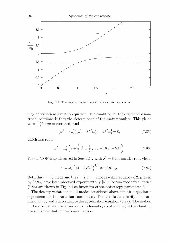
202 Dynamics of the condensate
Fig. 7.4 The mode frequencies (7.86) as functions of λ.
may be written as a matrix equation. The condition for the existence of non-trivial solutions is that the determinant of the matrix vanish. This yieldsω2 = 0 (for δn = constant) and
(ω2 − 4ω20)(ω
2 − 3λ2ω20) − 2λ2ω4
0 = 0, (7.85)
which has roots
ω2 = ω20
(2 +
32λ2 ± 1
2
√16 − 16λ2 + 9λ4
). (7.86)
For the TOP trap discussed in Sec. 4.1.2 with λ2 = 8 the smaller root yields
ω = ω0
(14 − 2
√29)1/2
≈ 1.797ω0. (7.87)
Both this m = 0 mode and the l = 2, m = 2 mode with frequency√
2ω0 givenby (7.83) have been observed experimentally [5]. The two mode frequencies(7.86) are shown in Fig. 7.4 as functions of the anisotropy parameter λ.
The density variations in all modes considered above exhibit a quadraticdependence on the cartesian coordinates. The associated velocity fields arelinear in x, y and z according to the acceleration equation (7.27). The motionof the cloud therefore corresponds to homologous stretching of the cloud bya scale factor that depends on direction.

7.3 Collective modes in traps 203
The scissors mode
In the Thomas–Fermi approximation there are modes having a simple ana-lytical form also for a general harmonic trap
V (r) =12m(ω2
xx2 + ω2yy
2 + ω2zz
2), (7.88)
where the frequencies ωx, ωy and ωz are all different. For traps with rota-tional symmetry about the z axis we have seen that there exist modes witha density variation proportional to xz or yz, the associated frequency beinggiven by ω2 = ω2
0(1+λ2). These modes are linear combinations of r2Y2,1 andr2Y2,−1, which are degenerate eigenstates. In addition there is a mode withfrequency given by ω2 = 2ω2
0 and a density variation proportional to xy,which is a linear combination of the modes with l = 2, m = ±2. Modes withdensity variations proportional to xy, yz or zx are purely two-dimensional,and also exist for a general harmonic trap with a potential given by (7.88).Let us consider a density change given by
δn = Cxy, (7.89)
where C is a coefficient which we assume varies as e−iωt. In order to deter-mine the velocity field associated with this mode we start with the hydro-dynamic equations in their original form. In the Thomas–Fermi approxima-tion, δμ = U0δn (see Eq. (7.59)) and therefore from Eq. (7.27) the velocityis given by
−imωv = −U0∇(Cxy) = −U0C(y, x, 0). (7.90)
Since ∇·v = 0, the continuity equation (7.26) reduces to
−iωδn = −(∇n) · v. (7.91)
We now use the condition for hydrostatic equilibrium of the unperturbedcloud, ∇n = −∇V/U0, and insert v from (7.90) on the right-hand side of(7.91) which becomes C(ω2
x + ω2y)xy/iω. This shows that the equations of
motion are satisfied provided
ω2 = ω2x + ω2
y . (7.92)
Corresponding results are obtained for density variations proportional to yz
and zx, with frequencies given by cyclic permutation of the trap frequenciesin (7.92).
The mode (7.89) is sometimes called a scissors mode, and it has beenobserved experimentally in a Bose–Einstein condensate [6]. The reason forthe name may be understood by considering the density change when the

204 Dynamics of the condensate
equilibrium cloud in the trap is rotated. The equilibrium density profile isproportional to 1−x2/R2
x−y2/R2y−z2/R2
z, where the lengths Ri are given by(6.33). A rotation of the cloud by an angle χ about the z axis correspondsto the transformation x → x cos χ − y sinχ, y → x sinχ + y cos χ. Thecorresponding change in the density for small χ is proportional to xy. Thedensity change in the mode is thus the same as would be produced by a rigidrotation of the cloud. However, the velocity field varies as (y, x, 0), and itis therefore very different from that for rigid rotation about the z axis,which is proportional to (−y, x, 0). The velocity of the condensate mustbe irrotational, and therefore the latter form of the velocity is forbidden.The name of the mode is taken from nuclear physics: in deformed nuclei,the density distributions of neutrons and protons can execute out-of-phaseoscillations of this type which resemble the opening and closing of a pair ofscissors. The scissors modes are purely two-dimensional, and therefore theirfrequencies do not depend on how the trapping potential varies in the thirddirection, provided it has the general form m(ω2
xx2 + ω2yy
2)/2 + V (z).
7.3.3 Collective coordinates and the variational method
In general it is not possible to solve the equations of motion for a trappedBose gas analytically and one must resort to other approaches, either nu-merical methods, or approximate analytical ones. In this section we con-sider low-lying excitations and describe how to calculate properties of modeswithin two related approximate schemes. We shall illustrate these methodsby applying them to the breathing mode of a cloud in a spherically symmet-ric trap, with a potential
V (r) =12mω2
0r2. (7.93)
In the notation of Sec. 7.3.1, this mode has l = 0 and radial index n = 1.
Collective coordinates
For the modes examined above in the Thomas–Fermi approximation theinteraction between particles plays an important role, and the motion ishighly collective. The idea behind the method of collective coordinates isto identify variables related to many particles that may be used to describethe collective behaviour. A simple example is the centre-of-mass coordinate,which may be used to describe the modes of frequency ωi in a harmonic trap.In Chapter 6 we showed how the width parameter R of a cloud may be usedas a variational parameter in determining an approximate expression for

7.3 Collective modes in traps 205
the energy. We now extend this approach to calculate the properties of thebreathing mode.
Let us assume that during the motion of the cloud, the density profilemaintains its shape, but that its spatial extent depends on time. Ratherthan adopting the Gaussian trial wave function used previously, we shalltake a more general one
ψ(r) =AN1/2
R3/2f(r/R)eiφ(r), (7.94)
where f is an arbitrary real function, and A, a number, is a normalizationconstant. The total energy of the cloud obtained by evaluating Eq. (6.9)may be written as
E = Eflow + U(R). (7.95)
Here the first term is the kinetic energy associated with particle currents,and is given by
Eflow =�
2
2m
∫dr|ψ(r)|2(∇φ)2. (7.96)
The second term is an effective potential energy, and it is equal to theenergy of the cloud when the phase does not vary in space. It is made upof a number of terms:
U(R) = Ezp + Eosc + Eint, (7.97)
where
Ezp =�
2
2m
∫dr(
d|ψ|dr
)2
= czpR−2 (7.98)
is the contribution from the zero-point kinetic energy,
Eosc =12mω2
0
∫drr2|ψ|2 = coscR
2 (7.99)
is that from the harmonic-oscillator potential, and
Eint =12U0
∫dr|ψ|4 = cintR
−3 (7.100)
is that due to interactions.3 The coefficients c, which are constants thatdepend on the choice of f , are defined by these equations. The equilibriumradius of the cloud R0 is determined by minimizing the total energy. The
3 Note that the total kinetic energy equals Ezp + Eflow.

206 Dynamics of the condensate
kinetic energy contribution (7.96) is positive definite, and is zero if φ is con-stant, and therefore the equilibrium condition is that the effective potentialbe a minimum,
dU
dR
∣∣∣∣R =R0
= 0, (7.101)
or, since the contributions to the energy behave as powers of R as shown inEqs. (7.98)–(7.100),
RdU
dR
∣∣∣∣R =R0
= −2Ezp + 2Eosc − 3Eint = 0. (7.102)
When R differs from its equilibrium value there is a force tending to changeR. To derive an equation describing the dynamics of the cloud, we need tofind the kinetic energy associated with a time dependence of R. ChangingR from its initial value to a new value R amounts to a uniform dilation ofthe cloud, since the new density distribution may be obtained from the oldone by changing the radial coordinate of each atom by a factor R/R. Thevelocity of a particle is therefore equal to
v(r) = rR
R, (7.103)
where R denotes the time derivative of R. The kinetic energy of the bulkmotion of the gas is thus given by
Eflow =m
2R2
R2
∫drn(r)r2
=12meffR2, (7.104)
where
meff = Nmr2
R2. (7.105)
Here r2 =∫
drn(r)r2/∫
drn(r) is the mean-square radius of the cloud. Notethat meff is independent of R. For a harmonic trap the integral here isidentical with that which occurs in the expression (7.99) for the contributionto the energy due to the oscillator potential, and therefore we may write
Eflow =R2
ω20R
2Eosc (7.106)
or
meff =2
ω20R
2Eosc. (7.107)
7.3 Collective modes in traps 207
The total energy of the cloud may thus be written as the sum of the energyof the static cloud Eq. (7.97) and the kinetic energy term Eq. (7.104),
E =12meffR2 + U(R), (7.108)
which is the same expression as for a particle of mass meff moving in a one-dimensional potential U(R). From the condition for energy conservation,dE/dt = 0, it follows that the equation of motion is
meffR = −∂U(R)∂R
. (7.109)
This equation is not limited to situations close to equilibrium, and in Sec.7.5 below we shall use it to determine the final velocity of a freely expandingcloud. However, as a first application we investigate the frequency of smalloscillations about the equilibrium state. Expanding the effective potentialto second order in R − R0, one finds
U(R) = U(R0) +12Keff(R − R0)2, (7.110)
where
Keff = U ′′(R0) (7.111)
is the effective force constant. Therefore the frequency of oscillations is givenby
ω2 =Keff
meff. (7.112)
This result is in fact independent of the trapping potential, but we shall nowspecialize our discussion to harmonic traps. From the expressions (7.98)–(7.100) one sees that
R2U ′′ = 6Ezp + 2Eosc + 12Eint
= 8Eosc + 3Eint, (7.113)
where the latter form follows from the first by using the virial condition Eq.(7.102) to eliminate the zero-point energy. Thus the frequency is given by
ω2 = ω20
[4 +
32
Eint(R0)Eosc(R0)
]. (7.114)
In Sec. 16.2 we shall apply this result to fermions.Let us examine a number of limits of this expression. First, when in-
teractions may be neglected one finds ω = ±2ω0, in agreement with theexact result, corresponding quantum-mechanically to two oscillator quanta.

208 Dynamics of the condensate
This may be seen from the fact that the Gross–Pitaevskii equation in theabsence of interactions reduces to the Schrodinger equation, and the energyeigenvalues are measured with respect to the chemical potential, which is3�ω0/2. The lowest excited state with spherical symmetry corresponds totwo oscillator quanta, since states having a single quantum have odd parityand therefore cannot have spherical symmetry.
Another limit is that of strong interactions, Na/aosc 1. The zero-pointenergy can be neglected to a first approximation, and the virial condition(7.102) then gives Eint(R0) = 2Eosc(R0)/3 and therefore
ω2 = 5ω20. (7.115)
This too agrees with the exact result in this limit, Eq. (7.72) for n = 1, l = 0.It is remarkable that, irrespective of the form of the function f , the mode
frequency calculated by the approximate method above agrees with the exactresult in the limits of strong interactions and of weak interactions. Thiscircumstance is a special feature of the harmonic-oscillator potential, forwhich the effective mass is simply related to the potential energy due to thetrap.
The method may be applied to anisotropic traps by considering pertur-bations of the cloud corresponding to transformations of the form x, y, z →αx, βy, γz, where the scale factors may be different. This gives three cou-pled equations for α, β and γ. For an axially symmetric trap this leads toEqs. (7.83) and (7.86) for the mode frequencies. Likewise the properties ofthe scissors modes may be derived by considering displacements of the formx → x + ay, y → y + bx, z → z and cyclic permutations of this.
Variational approach
The calculation of mode frequencies based on the idea of collective coordi-nates may be put on a more formal footing by starting from the variationalprinciple Eq. (7.4). The basic idea is to take a trial function which dependson a number of time-dependent parameters and to derive equations of mo-tion for these parameters by applying the variational principle [7]. As anexample, we again consider the breathing mode of a cloud in a sphericaltrap. The amplitude of the wave function determines the density distribu-tion, while its phase determines the velocity field. For the amplitude wetake a function of the form we considered above in Eq. (7.94). In the cal-culation for the breathing mode we assumed that the velocity was in theradial direction and proportional to r. Translated into the behaviour of thewave function, this implies that the phase of the wave function varies as

7.3 Collective modes in traps 209
r2, since the radial velocity of the condensate is given by (�/m)∂φ/∂r. Wetherefore write the phase of the wave function as βmr2/2�, where β is asecond parameter in the wave function. The factor m/� is included to makesubsequent equations simpler. The complete trial wave function is thus
ψ(r, t) =AN1/2
R3/2f(r/R)eiβmr2/2�. (7.116)
We now carry out the integration over r in (7.5) and obtain the La-grangian as a function of the two independent variables β and R and thetime derivative β,
L = −(
U(R) +meffR2
2(β2 + β)
). (7.117)
From the Lagrange equation for β,
d
dt
∂L
∂β=
∂L
∂β(7.118)
we find
β =R
R. (7.119)
This is the analogue of the continuity equation for this problem, since itensures consistency between the velocity field, which is proportional to β
and the density profile, which is determined by R. The Lagrange equationfor R is
d
dt
∂L
∂R=
∂L
∂R, (7.120)
which reduces to ∂L/∂R = 0, since the Lagrangian does not depend on R.This is
meffR(β + β2) = −∂U(R)∂R
. (7.121)
When Eq. (7.119) for β is inserted into (7.121) we arrive at the equation ofmotion (7.109) derived earlier. The results of this approach are equivalent tothose obtained earlier using more heuristic ideas. However, the variationalmethod has the advantage of enabling one to systematically improve thesolution by using trial functions with a greater number of parameters.
Finally, let us compare these results for the breathing mode with thoseobtained in Eq. (7.72) by solving the hydrodynamic equations with the quan-tum pressure term neglected. The hydrodynamic equations are valid in thelimit Ezp Eint, and therefore in the results for the collective coordinateand variational approaches we should take that limit. As already mentioned,

210 Dynamics of the condensate
the lowest l = 0 mode involves a uniform change in the density everywhereand has zero frequency because such a density change produces no restor-ing forces. This corresponds to the index n in (7.72) being zero. The firstexcited state with l = 0 corresponds to n = 1, indicating that the densityperturbation has a single radial node. According to (7.72) the frequencyof the mode is given by ω2 = 5ω2
0, in agreement with the result of the col-lective coordinate approach, Eq. (7.115). The nature of the mode may bedetermined either from the general expression in terms of hypergeometricfunctions or by construction, as we shall now demonstrate.
The s-wave solutions to (7.65) satisfy the equation
ω2δn = ω20r
d
drδn − ω2
0
(R2 − r2)2r
d2
dr2(rδn). (7.122)
Following the method used earlier for anisotropic traps, let us investigatewhether there exists a solution of the form
δn = A + Br2, (7.123)
where A and B are constants to be determined. This function is the analogueof Eq. (7.84) for a mode with spherical symmetry (B = C). Inserting thisexpression into (7.122), we find from the terms proportional to r2 that
ω2 = 5ω20, (7.124)
in agreement with the values calculated by other methods, as given in (7.72)and (7.115). By equating the terms independent of r we obtain the condition
B = −53
A
R2. (7.125)
The density change δn is thus given by
δn = A
(1 − 5r2
3R2
). (7.126)
This is identical with the density change of the equilibrium cloud producedby a change in R. To show this, we use the fact that in the Thomas–Fermi approximation, when the zero-point kinetic energy is neglected, theequilibrium density is given by
n =C1
R3
(1 − r2
R2
), (7.127)
where C1 is a constant. From (7.127) it follows that a small change δR in
7.4 Surface modes 211
the cloud radius R gives rise to a density change
δn = −C1
R4
(3 − 5
r2
R2
)δR, (7.128)
which has the same form as Eq. (7.126). The corresponding velocity fieldmay be found from the continuity equation (7.8), which shows that v ∝ ∇δn,which is proportional to r. Thus the velocity field is homologous, as wasassumed in our discussion of modes in terms of collective coordinates.
7.4 Surface modes
In the previous section we showed that in a spherically symmetric trap thereare modes that are well localized near the surface of the cloud. To shedlight on these modes, we approximate the potential in the surface regionby a linear function of the coordinates, as we did in our study of surfacestructure in Sec. 6.3, and write
V (r) = Fx, (7.129)
where the coordinate x measures distances in the direction of ∇V . Thisapproximation is good provided the spatial extent of the mode in the radialdirection is small compared with the linear dimensions of the cloud. As weshall see, this condition is equivalent to the requirement that the wavelengthof the excitation is small compared with the linear dimensions. FollowingRef. [8] we now investigate surface modes for a condensate in the linearramp potential (7.129). Because of the translational invariance in the y andz directions the solution may be chosen to have the form of a plane wavefor these coordinates. We denote the wave number of the mode by q, andtake the direction of propagation to be the z axis. Provided the mode is notconcentrated in the surface region of thickness δ given by Eq. (6.44), we mayuse the Thomas–Fermi approximation, in which the equilibrium condensatedensity n is given by n(x) = −Fx/U0 for x < 0, while it vanishes for x > 0.Equation (7.63) for the density oscillation in the mode has a solution
δn = Ceqx+iqz, (7.130)
C being an arbitrary constant. This describes a wave propagating on thesurface and decaying exponentially in the interior. For the Thomas–Fermiapproximation to be applicable the decay length 1/q must be much greaterthan δ. Since (7.130) satisfies the Laplace equation, ∇2δn = 0, we obtain

212 Dynamics of the condensate
by inserting (7.130) into (7.63) the dispersion relation
ω2 =F
mq. (7.131)
This has the same form as that for a gravity wave propagating on the surfaceof an incompressible ideal fluid in the presence of a gravitational field g =F/m.
The solution (7.130) is however not the only one which decays exponen-tially in the interior. To investigate the solutions to (7.63) more generallywe insert a function of the form
δn = f(qx)eqx+iqz, (7.132)
and obtain the following second-order differential equation for f(y),
yd2f
dy2+ (2y + 1)
df
dy+ (1 − ε)f = 0, (7.133)
where ε = mω2/Fq. By introducing the new variable z = −2y one sees thatEq. (7.133) becomes the differential equation for the Laguerre polynomialLn(z), provided ε − 1 = 2n. We thus obtain the general dispersion relationfor the surface modes
ω2 =F
mq(1 + 2n), n = 0, 1, 2, . . . (7.134)
The associated density oscillations are given by
δn(x, z, t) = CLn(−2qx)eqx+iqz−iωt, (7.135)
where C is a constant.Let us now compare the frequencies of these modes with those given in
Eq. (7.72) for the modes of a cloud in an isotropic, harmonic trap. For l
much greater than n, the dispersion relation becomes ω2 = ω20l(1 + 2n).
Since the force due to the trap at the surface of the cloud is F = ω20R per
unit mass and the wave number of the mode at the surface of the cloud isgiven by q = l/R, it follows that ω2
0l = Fq/m and the dispersion relationω2 = ω2
0l(1 + 2n) is seen to be in agreement with the result (7.134) for theplane surface. For large values of l it is thus a good approximation to replacethe harmonic-oscillator potential by the linear ramp. The surface modes areconcentrated within a distance of order (2n + 1)R/l from the surface, andtherefore provided this is smaller than R, it is permissible to approximatethe harmonic-oscillator potential by the linear ramp. It should be notedthat the frequencies of the n = 0 modes for the linear ramp potential agreewith the frequencies of the nodeless radial modes (corresponding to n = 0)

7.5 Free expansion of the condensate 213
for a harmonic trap at all values of l. For modes with radial nodes (n �= 0),the two results agree only for l n.
The results above were obtained in the Thomas–Fermi approximation,which is valid only if the depth to which the mode penetrates is much greaterthan the scale of the surface structure δ, Eq. (6.44). At shorter wavelengths,there are corrections to the dispersion relation (7.131) which may be relatedto an effective surface tension due to the kinetic energy of matter in thesurface region [8]. Surface excitations for l = 2 and l = 4 have been observedexperimentally by using as a stirrer the dipole force due to a laser beam [9](see Sec. 4.2.1).
7.5 Free expansion of the condensate
The methods described above are not limited to situations close to equilib-rium. One experimentally relevant problem is the evolution of a cloud ofcondensate when the trap is switched off suddenly. The configuration of thecloud after expansion is used as a probe of the cloud when it is impossibleto resolve its initial structure directly. For simplicity, we consider a cloudcontained by an isotropic harmonic trap, V (r) = mω2
0r2/2, which is turned
off at time t = 0. We employ a trial function of the form (7.116) withf(r/R) = exp(−r2/2R2). As may be seen from Eq. (6.19), the zero-pointenergy is given by
Ezp =3N�
2
4mR2(7.136)
and the interaction energy by
Eint =N2U0
2(2π)3/2R3. (7.137)
For the Gaussian trial function the effective mass (Eq. (7.107)) is meff =3Nm/2. The energy conservation condition therefore yields
3mR2
4+
3�2
4mR2+
12(2π)3/2
NU0
R3=
3�2
4mR(0)2+
12(2π)3/2
NU0
R(0)3, (7.138)
where R(0) is the radius at time t = 0.In the absence of interactions (U0 = 0) we may integrate (7.138) with the
result
R2(t) = R2(0) + v20t
2, (7.139)
where v0, which is equal to the root-mean-square particle velocity, is given

214 Dynamics of the condensate
by
v0 =�
mR(0). (7.140)
Thus the expansion velocity is of order the velocity uncertainty predicted bythe Heisenberg uncertainty principle for a particle confined within a distance∼ R(0). The initial radius, R(0), is equal to the oscillator length aosc =(�/mω0)1/2, and therefore the result (7.139) may be written as
R2(t) = R2(0)(1 + ω20t
2). (7.141)
This agrees with the result obtained previously in Eq. (2.58) for the evolutionof a Gaussian wave packet.
When interactions are present, the development of R as a function of timemay be found by numerical integration. However, the asymptotic behaviourfor t → ∞ may be obtained using the energy conservation condition (7.138),which yields a final velocity given by
v2∞ =
�2
m2R(0)2+
U0N
3(2π3)1/2mR(0)3. (7.142)
When Na/aosc is large, the initial size of the cloud may be determined byminimizing the sum of the oscillator energy and the interaction energy. Ac-cording to (6.27) the result for an isotropic trap is
R(0) =(
2π
)1/10(Na
aosc
)1/5
aosc. (7.143)
At large times, the cloud therefore expands according to the equation
R2(t)R2(0)
� U0N
3(2π3)1/2mR(0)5t2 =
23ω2
0t2, (7.144)
since the final velocity is dominated by the second term in (7.142).From an experimental point of view, an important observable is the shape
after expansion of a cloud initially confined by an anisotropic trap. Thisproblem may be studied quantitatively by generalizing the approach of thissubsection to an anisotropic cloud, and this is the subject of Problem 7.4.The tighter the confinement of the cloud in a given direction, the greaterthe pressure gradient due to the mean-field energy, and the greater the finalvelocity of expansion in that direction. Thus initially prolate clouds becomeoblate, and vice versa, just as they do for non-interacting gases, as describedin Sec. 2.3.

7.6 Solitons 215
7.6 Solitons
In the dynamical problems addressed so far, we have obtained analyti-cal results for small-amplitude motions, but have had to rely on approx-imate methods when non-linear effects are important. However the time-dependent Gross–Pitaevskii equation has exact analytical solutions in thenon-linear regime. These have the form of solitary waves, or solitons, that is,localized disturbances which propagate without change of form.4 The sub-ject of solitons has a long history, starting with the observations on shallowwater waves made by the British engineer and naval architect John ScottRussell in the decade from 1834 to 1844. Soliton solutions exist for a num-ber of non-linear equations, among them the Korteweg–de Vries equation,which describes the properties of shallow water waves, and the non-linearSchrodinger equation, of which the Gross–Pitaevskii equation (7.1) is a spe-cial case.
The physical effects that give rise to the existence of solitons are non-linearity and dispersion. Both of these are present in the Gross–Pitaevskiiequation, as one can see by examining the Bogoliubov dispersion relationgiven by (7.31), ω2 = (nU0/m)q2+�
2q4/4m2 , which exhibits the dependenceof the velocity of an excitation on the local density and on the wave number.Solitons preserve their form because the effects of non-linearity compensatefor those of dispersion. Before describing detailed calculations, we makesome general order-of-magnitude arguments. For definiteness, let us considera spatially uniform condensed Bose gas with repulsive interactions. If alocalized disturbance of the density has an amplitude Δn and extends overa distance L, it may be seen from the dispersion relation that the velocityof sound within the disturbance is different from the sound velocity in thebulk medium by an amount ∼ s(Δn)/n due to non-linear effects. One canalso see that, since q ∼ 1/L, dispersion increases the velocity by an amount∼ sξ2/L2, where ξ is the coherence length, given by (6.62). For the effects ofnon-linearity to compensate for those of dispersion, these two contributionsmust cancel. Therefore the amplitude of the disturbance is related to itslength by
Δn
n∼ − ξ2
L2. (7.145)
The velocity u of the disturbance differs from the sound speed by an amount
4 In the literature, the word ‘soliton’ is sometimes used to describe solitary waves with specialproperties, such as preserving their shapes when they collide with each other. We shall followthe usage common in the field of Bose–Einstein condensation of regarding the word ‘soliton’ asbeing synonymous with solitary wave.

216 Dynamics of the condensate
of order the velocity shifts due to dispersion and non-linearity, that is
|u − s| ∼ sξ2
L2. (7.146)
Note that solitons for this system correspond to density depressions, whereasfor waves in shallow water, they correspond to elevations in the water level.This difference can be traced to the fact that the dispersion has the oppositesign for waves in shallow water, since for these ω2 � ghq2[1−(qh)2/3], whereg is the acceleration due to gravity and h the equilibrium depth of the water.The non-linearity has the same sign in the two cases, since the velocity ofsurface waves increases with the depth of the water, just as the speed ofsound in a Bose gas with repulsive interactions increases with density.
Solitons are also observed in non-linear optics, and the intensity of thelight plays a role similar to that of the condensate density in atomic clouds.By analogy, the word dark is used to describe solitons that correspond todensity depressions. This category of solitons is further divided into blackones, for which the minimum density is zero, and grey ones, for which itis greater than zero. Solitons with a density maximum are referred to asbright.
7.6.1 Dark solitons
For repulsive interactions between particles, the simplest example of a solitonis obtained by extending to the whole of space the stationary solution to theGross–Pitaevskii equation at a wall found in Sec. 6.4 (see Eq. (6.65)),
ψ(x) = ψ0 tanh(
x√2ξ
)(7.147)
with
ξ =�
(2mn0U0)1/2(7.148)
being the coherence length far from the wall. This solution is static, andtherefore corresponds to a soliton with velocity zero. It is also referred toas a kink, since the phase of the wave function jumps discontinuously by π
as x passes through zero.The Gross–Pitaevskii equation (7.1) possesses one-dimensional soliton so-
lutions for which the associated density depends on the spatial coordinatex and the time t through the combination x−ut. For repulsive interactions(U0 > 0) we look for solutions where the density n approaches a non-zero

7.6 Solitons 217
value n0 when x → ±∞. We insert into (7.1) a solution of the form
ψ(x, t) = f(x − ut)e−iμt/� (7.149)
and obtain the following differential equation for the function f ,
− �2
2mf ′′ + U0|f |2f = −i�uf ′ + μf. (7.150)
Here f ′ denotes the derivative of f with respect to the variable x − ut.The chemical potential μ = U0n0 is determined by the background densityn0 = f2
0 , where f0 denotes the amplitude of the condensate wave functionfor x → ±∞.
We separate the solution to (7.150) into real and imaginary parts by writ-ing
f = f0[α(x) + iβ(x)], (7.151)
where α and β are real functions of the dimensionless variable x = (x−ut)/ξ.When x → ±∞ the functions α and β approach the values α(±∞) andβ(±∞), respectively, where
α(±∞)2 + β(±∞)2 = 1. (7.152)
Let us consider possible solutions for which the imaginary part is equal toa constant everywhere, β = β0, and separate the equation (7.150) into realand imaginary parts. This yields the two equations
α′′ + (1 − α2 − β20)α = 0 (7.153)
and
(1 − α2 − β20)β0 =
√2u
sα′, (7.154)
where s = (n0U0/m)1/2 is the sound velocity of the uniform condensate, andthe prime denotes differentiation with respect to x. First we ensure the con-sistency of the two equations by multiplying (7.153) by α′ and integrating,using the boundary condition α(±∞)2 = 1 − β2
0 . This results in
2(α′)2 = (1 − α2 − β20)2, (7.155)
which is consistent with (7.154) if
β20 =
u2
s2. (7.156)

218 Dynamics of the condensate
By comparing (7.153) with (6.64) and its solution (6.65) we conclude that theequation (7.154) and the boundary conditions are satisfied by the function
α = α0 tanh[(x − ut)α0√
2ξ
](7.157)
with
α0 =√
1 − β20 =
√1 − u2
s2. (7.158)
The soliton wave function is thus
ψ =√
n0
[iu
s+
√(1 − u2
s2) tanh
(x − ut√
2ξu
)]e−iμt/� (7.159)
with the associated density
n = n0(α2 + β20) = n0
[u2
s2+ (1 − u2
s2) tanh2
(x − ut√
2ξu
)]
= n0 − (n0 − nmin)1
cosh2[(x − ut)/√
2ξu]. (7.160)
Here we have introduced the width ξu, which depends on velocity accordingto the equation
ξu =ξ
[1 − (u/s)2]1/2(7.161)
and the minimum density,
nmin = n0u2
s2. (7.162)
Equation (7.162) shows that the soliton velocity u is given by (nminU0/m)1/2,which is the bulk sound velocity evaluated at the density nmin. When u = 0the minimum density in the soliton vanishes, and the density profile (7.160)reduces to that associated with (7.147). These analytical results, whichwere derived by Tsuzuki [10], confirm the qualitative estimates (7.145) and(7.146) arrived at earlier.
The velocity field v associated with the moving soliton may be founddirectly from the phase φ of the wave function (7.159) as v = (�/m)∂φ/∂x.As an alternative derivation we shall use the continuity equation to expressv in terms of the density. Since ∂n/∂t = −u∂n/∂x, the continuity equationassumes the form
∂
∂x(un − vn) = 0, (7.163)

7.6 Solitons 219
–5 –4 –3 –2 –1 0 1 2 3 4 5–2.5
–2–1.5
–1–0.5
00.5
11.5
(x – ut)/u
v/u
n/n0
Fig. 7.5 The density and the velocity field of a dark soliton for u2 = 0.3s2.
which upon integration and use of the boundary condition that the velocityfield vanishes at infinity becomes
v = u(1 − n0
n
). (7.164)
The density and velocity field of a dark soliton are plotted in Fig. 7.5 foru2 = 0.3s2. The phase φ of the wave function is φ = tan−1(β0/α). The totalchange Δφ in phase across the soliton is
Δφ = φ(∞) − φ(−∞) = tan−1 β0
α0−(
π − tan−1 β0
α0
)= −2 cos−1
(u
s
).
(7.165)
For a dark soliton moving in the positive x direction the phase changeis negative. Physically this is because the wave is a density depressionand consequently the fluid velocity associated with it is in the negative x
direction as shown by (7.164).The total energy of the soliton may be obtained from (7.159). To allow for
the deficit of particles in the soliton it is convenient to consider the quantityE − μN rather than the energy E itself. In the absence of the soliton thecorresponding density is U0n
20/2− μn0. The difference Δ(E − μN) between
220 Dynamics of the condensate
E − μN with and without the soliton is thus
Δ(E − μN) = A∫ ∞
−∞dx
[�
2
2m
∣∣∣∣dψ
dx
∣∣∣∣2
+12U0(|ψ|4 − n2
0) − μ(|ψ|2 − n0)
],
(7.166)with A being the cross-sectional area in the plane perpendicular to thedirection of propagation. Since we are considering only a single soliton,the chemical potential μ is given by its value in the absence of the soliton,μ = U0n0, and the soliton energy per unit cross-sectional area can thereforebe written as
Esol =Δ(E − μN)
A =∫ ∞
−∞dx
[�
2
2m
∣∣∣∣dψ
dx
∣∣∣∣2
+12U0(|ψ|2 − n0)2
]. (7.167)
When (7.159) is inserted into this expression and use is made of the integral∫∞−∞ dx/ cosh4 x = 2/3, one finds that the two terms in (7.167) contribute
equally to the soliton energy per unit area which can be written as
Esol =43n0�s
(1 − u2
s2
)3/2
. (7.168)
Note that the soliton energy decreases with increasing velocity, corre-sponding to a negative effective mass, as defined by the expansion of (7.168)for u s,
Esol �43n0�s − 2n0�s
u2
s2, (7.169)
which shows that the effective mass per unit area equals −4n0�/s. Thedeficit of particles ΔN (per unit cross-sectional area) associated with thesoliton is readily obtained from the density expression (7.160). It is ΔN =2√
2n0ξ(1 − u2/s2)1/2, which vanishes as u approaches the sound velocity.The energy per (deficit) particle Esol/ΔN is thus of order the chemicalpotential times (1 − u2/s2).
The expression (7.168) can be written in the alternative fashion
Esol =4
3√
mU0(μ − mu2)3/2, (7.170)
which allows us to draw some interesting conclusions regarding soliton dy-namics. Dark solitons in external potentials behave essentially like particles,if the potential varies sufficiently slowly in space [11]. To see this we consideradding a slowly varying potential V (x). In the Thomas–Fermi approxima-tion, the chemical potential and the external potential are related to the localdensity n0(x) in the absence of the soliton by Eq. (6.31), μ = V (x)+n0(x)U0.

7.6 Solitons 221
This suggests that the energy (7.170) in the presence of a slowly varying ex-ternal potential is modified according to the expression
Esol =4
3√
mU0[μ − V (xs) − mu2(xs)]3/2, (7.171)
where xs denotes the position of the soliton centre (recall that the solitonvelocity according to (7.160) equals the local sound velocity at the centrex = ut).
From Eq. (7.171) one sees that for energy to be conserved, the quantityμ− V (xs)−mu2(xs) must be constant, implying that V (xs) + mu2(xs) is aconstant, independent of xs. The latter expression is the energy of a particleof mass 2m. Consequently, we arrive at the remarkable conclusion that themotion of a soliton in a Bose–Einstein condensate in an external potentialis the same as that of a particle of mass 2m in the same potential. Thus, fora potential having a minimum, the period of the motion of a soliton is
√2
times that of a particle of mass m in the potential, the energy of the particlebeing equal to the value of the external potential at the turning points ofthe motion.
Because of the inhomogeneity of the potential, the form of the velocitythat we have adopted is not an exact solution of the equation of motion, andas the soliton accelerates due to the external potential, it will emit soundwaves in much the same way as a charged particle emits electromagneticradiation when accelerated. However, this effect is small if the potentialvaries sufficiently slowly. Dissipation tends to make the soliton less dark,that is to reduce the depth of the density depression. In a condensate offinite extent, such as one in a trap, emission of phonons is suppressed by thediscrete nature of the spectrum of elementary excitations.
Experimentally, dark solitons in Bose–Einstein condensates were first gen-erated by the method of phase imprinting (Sec. 13.4) at the National Insti-tute of Standards and Technology (NIST) [12] and in Hannover [13].
The Gross–Pitaevskii equation also has solutions representing periodicarrays of solitons. If D denotes the period of the array, the solution for aunit cell of the array may be obtained by the same method as for a singlesoliton, except that the derivative f ′ of the modulus of the condensate wavefunction vanishes at x − ut = ±D/2 instead of for x − ut → ±∞ as itdoes for a single soliton in an infinite condensate. The solution for thewhole array is then obtained by joining together solutions for a single cellby matching ψ at the boundary between successive cells. These solutionswere also discussed by Tsuzuki [10], and in Sec. 14.4.1 we shall return to
222 Dynamics of the condensate
them in connection with the description of loops in the band structure fora Bose–Einstein condensate moving in an optical lattice.
7.6.2 Bright solitons
For attractive interactions (U0 < 0) there are also one-dimensional solitonsolutions with a maximum instead of a minimum in the density. These arereferred to as bright solitons. Their properties differ from those of darksolitons in that their height and width are unrelated to their propagationvelocity. For vanishing soliton velocity (u = 0) Eq. (7.150) admits a solutionof the form
f =b
cosh ax, (7.172)
provided a and b satisfy
a2 = −2mμ
�2and b2 =
2μ
U0. (7.173)
It is clearly necessary that μ < 0 and U0 < 0 for this solution to exist. Thecondensate wave function describing a bright soliton at rest is thus given by
ψ(x, t) =(
2μ
U0
)1/2 1cosh[(2m|μ|/�2)1/2x]
e−iμt/�. (7.174)
In contrast to the case of a dark soliton, the density vanishes at large dis-tances from the centre.
There exists an infinity of solutions to the one-dimensional Gross–Pitaevskii equation which differ from (7.174) by a Galilean transformation,that is the substitution x → x − ut − x0 in the argument of the hyperbolicfunction, multiplication by the phase factor exp(imux/�) and the replace-ment μ → μ − mu2/2. This may be seen directly by inserting a solution ofthis form in the differential equation (7.150). Note that while the velocity ofa dark soliton cannot exceed the sound velocity, there is no correspondingrestriction on the velocity of bright solitons.
Bright solitons have been generated in experiments involving condensatesof 7Li atoms in the hyperfine state F = 1, mF = 1 with the use of amagnetic field to tune the scattering length in the vicinity of a Feshbachresonance [14, 15]. In the experiment [14] soliton trains containing severalsolitons were formed, allowing the study of the repulsive interaction betweenneighbouring solitons. For atoms in an optical lattice it is possible to observebright solitons even in condensates with repulsive interactions [16]. Thereason is that the effective mass of an atom in an optical lattice becomes

7.6 Solitons 223
negative near the Brillouin zone boundary (see Sec. 14.2.3). As one can seefrom (7.150), a change in sign of the mass m will have the same effect as achange in sign of U0 in allowing for the existence of bright soliton solutions.
In bulk matter, purely one-dimensional solitons are unstable to perturba-tions in the other dimensions. This may be shown by studying small depar-tures of the condensate wave function from its form for a soliton, just as weearlier investigated oscillations of a condensate about the ground-state solu-tion. The corresponding equations are the Bogoliubov equations (7.39) and(7.40) with ψ(r, t) put equal to the solution for a soliton. For dark solitons ina condensate with repulsive interactions, this instability was demonstratedin Ref. [17]. When the instability grows, solitons break up into pairs of vor-tices. Bright solitons in a medium with attractive interactions are unstablewith respect to a periodic spatial variation in the transverse direction [18].This corresponds to a tendency to break up into small clumps, since theattractive interaction favours more compact structures, as discussed in Sec.6.2.
Problems
Problem 7.1 Derive the hydrodynamic equations (7.8) and (7.19) directlyfrom the action principle (7.4) with the Lagrangian (7.5), by varying theaction with respect to the magnitude and the phase of the condensate wavefunction ψ(r, t) = f(r, t)eiφ(r,t).
Problem 7.2 Show that for a harmonic trap with an axis of symmetrythere exist collective modes of the form (7.81), and verify the result (7.82)for their frequencies.
Problem 7.3 Consider a trap with axial symmetry, corresponding to thepotential (7.75) with λ �= 1. Use the variational method with a trial functionof the form
ψ = Ce−ρ2/2R2e−z2/2Z2
eiαρ2m/2�eiβz2m/2�,
R, Z, α and β being variational parameters, to obtain equations of motionfor R and Z and identify the potential U(R, Z). Determine the frequenciesof small oscillations around the equilibrium state and compare the resultswith the frequencies (7.86) obtained by solving the hydrodynamic equationsin the Thomas–Fermi approximation.
Problem 7.4 Use the trial function given in Problem 7.3 to study the freeexpansion of a cloud of condensate upon release from an axially symmetrictrap of the form (7.75) with λ �= 1, by numerically solving the coupled

224 Dynamics of the condensate
differential equations for R and Z. Check that your numerical results satisfythe energy conservation condition.
Problem 7.5 Determine the density profile associated with a dark solitondirectly from (7.27) by making use of the fact that, since the form of thesoliton remains unchanged in a frame moving with velocity u, ∂v/∂t =−u∂v/∂x. Eliminate v by means of the continuity equation (7.163) to showthat the density satisfies the equation(
�
2ms
dn
dx
)2
=(
n
n0− u2
s2
)(n0 − n)2,
where x = x − ut. Integrate this equation to find the density profile.
References[1] N. N. Bogoliubov, J. Phys. (USSR) 11, 23 (1947), reprinted in D. Pines, The
Many-Body Problem, (New York, W. A. Benjamin, 1961), p. 292.[2] R. P. Feynman, Phys. Rev. 91, 1301 (1953); 94, 262 (1954).[3] S. Stringari, Phys. Rev. Lett. 77, 2360 (1996).[4] I. S. Gradshteyn and I. M. Ryzhik, Table of Integrals, Series and Products,
Fifth edition, (San Diego, Academic Press, 1994), 9.100.[5] D. S. Jin, J. R. Ensher, M. R. Matthews, C. E. Wieman, and E. A. Cornell,
Phys. Rev. Lett. 77, 420 (1996).[6] O. Marago, S. A. Hopkins, J. Arlt, E. Hodby, G. Hechenblaikner, and
C. J. Foot, Phys. Rev. Lett. 84, 2056 (2000).[7] Y. Castin and R. Dum, Phys. Rev. Lett. 77, 5315 (1996).[8] U. Al Khawaja, C. J. Pethick, and H. Smith, Phys. Rev. A 60, 1507 (1999).[9] R. Onofrio, D. S. Durfee, C. Raman, M. Kohl, C. E. Kuklewicz, and
W. Ketterle, Phys. Rev. Lett. 84, 810 (2000).[10] T. Tsuzuki, J. Low Temp. Phys. 4, 441 (1971).[11] T. Busch and J. R. Anglin, Phys. Rev. Lett. 84, 2298 (2000).[12] J. Denschlag, J. E. Simsarian, D. L. Feder, C. W. Clark, L. A. Collins,
J. Cubizolles, L. Deng, E. W. Hagley, K. Helmerson, W. P. Reinhardt,S. L. Rolston, B. I. Schneider, and W. D. Phillips, Science 287, 97 (2000).
[13] S. Burger, K. Bongs, S. Dettmer, W. Ertmer, K. Sengstock, A. Sanpera,G. V. Shlyapnikov, and M. Lewenstein, Phys. Rev. Lett. 83, 5198 (1999).
[14] K. E. Strecker, G. B. Partridge, A. G. Truscott, and R. G. Hulet, Nature417, 150 (2002).
[15] L. Khaykovich, F. Schreck, G. Ferrari, T. Bourdel, J. Cubizolles, L. D. Carr,Y. Castin, and C. Salomon, Science 296, 1290 (2002).
[16] B. Eiermann, T. Anker, M. Albiez, M. Taglieber, P. Treutlein, K.-P. Marzlin,and M. K. Oberthaler, Phys. Rev. Lett. 92, 230401 (2004).
[17] E. A. Kuznetsov and S. K. Turitsyn, Zh. Eksp. Teor. Fiz. 94, 119 (1988)[Sov. Phys.-JETP 67, 1583 (1988)].
[18] V. E. Zakharov and A. M. Rubenchik, Zh. Eksp. Teor. Fiz. 65, 997 (1973)[Sov. Phys.-JETP 38, 494 (1974)].
8
Microscopic theory of the Bose gas
In Chapter 7 we studied elementary excitations of the condensate using theGross–Pitaevskii equation, in which the wave function of the condensate istreated as a classical field. In this chapter we develop the microscopic theoryof the Bose gas, taking into account the quantum nature of excitations. Firstwe discuss the excitation spectrum of a homogeneous gas at zero temperature(Sec. 8.1) within the Bogoliubov approximation and determine the depletionof the condensate and the change in ground-state energy. Following thatwe derive in Sec. 8.2 the Bogoliubov equations for inhomogeneous gases.Excitations at non-zero temperatures are the subject of Sec. 8.3, where wedescribe the Hartree–Fock and Popov approximations, which are mean-fieldtheories.
The starting point for our calculations is the Hamiltonian (6.3). In termsof creation and annihilation operators for bosons, ψ†(r) and ψ(r) respec-tively, it has the form1
H =∫
dr[−ψ†(r)
�2
2m∇2ψ(r) + V (r)ψ†(r)ψ(r) +
U0
2ψ†(r)ψ†(r)ψ(r)ψ(r)
].
(8.1)As we have discussed in Chapter 5, the use of this simplified Hamiltonianwith an effective contact interaction of the form (5.34) is restricted to lowenergies and momenta. In the following we shall only consider the case ofrepulsive interaction, U0 > 0. In the Gross–Pitaevskii equation one worksnot with creation and annihilation operators but with the wave functionfor the condensed state, which is a classical field. The Gross–Pitaevskiiapproach is thus analogous to the classical theory of electrodynamics, in
1 In this and the following chapters we put a ‘hat’ on creation and annihilation operators as wellas on other operators when these are expressed in their second-quantized form.
225

226 Microscopic theory of the Bose gas
which a state is characterized by classical electric and magnetic fields, ratherthan by creation and annihilation operators for photons.
To take into account quantum fluctuations about the state in which allatoms are condensed in a single quantum state it is natural to write
ψ(r) = ψ(r) + δψ(r). (8.2)
If the fluctuation term δψ(r) is neglected, the Hamiltonian is equivalent tothe energy expression which leads to the Gross–Pitaevskii equation.
8.1 The uniform Bose gas
As a first illustration we consider a uniform gas of N interacting bosonscontained in a box of volume V . We express the creation and annihilationoperators occurring in (8.1) in terms of operators that create and destroyparticles in momentum states by the transformation2
ψ(r) =1
V 1/2
∑p
eip·r/�ap =V 1/2
(2π�)3
∫dpeip·r/�ap, (8.3)
where V is the volume, and its inverse
ap =1
V 1/2
∫dre−ip·r/�ψ(r). (8.4)
The Hamiltonian (8.1) then becomes
H =∑p
ε0pa†pap +
U0
2V
∑p,p′,q
a†p+qa†p′−qap′ ap, (8.5)
where ε0p = p2/2m. The operators ap and a†p that destroy and create bosonsin the state with momentum p satisfy the Bose commutation relations
[ap, a†p′ ] = δp,p′ , [ap, ap′ ] = 0, and [a†p, a†p′ ] = 0. (8.6)
We assume that in the interacting system the lowest-lying single-particlestate is macroscopically occupied in the sense that the expectation value ofthe particle number operator for the lowest-lying state becomes of order N
in the thermodynamic limit when N and V tend to infinity in such a waythat the density N/V remains constant. In the unperturbed system we have
a†0|N0〉 =√
N0 + 1|N0 + 1〉 and a0|N0〉 =√
N0|N0 − 1〉, (8.7)
and in the Hamiltonian we therefore replace a0 and a†0 by√
N0, as was first2 Note that with our convention for the Fourier transformation given in Sec. 5.2.1 this implies
that the operator a is the Fourier transform of ψ/V 1/2.

8.1 The uniform Bose gas 227
done by Bogoliubov [1]. This is equivalent to using Eq. (8.2) with the wavefunction for the condensed state given by ψ =
√N0φ0, where φ0 = V −1/2 is
the wave function for the zero-momentum state.Within the Bogoliubov approach one assumes that δψ(r) is small and
retains in the interaction all terms which have (at least) two powers of ψ(r)or ψ∗(r). This is equivalent to including terms which are no more thanquadratic in δψ(r) and δψ†(r), that is in ap and a†p for p �= 0. One finds
H =N2
0 U0
2V+∑
p(p�=0)
(ε0p +2n0U0)a†pap +n0U0
2
∑p(p�=0)
(a†pa†−p + apa−p), (8.8)
where n0 = N0/V is the density of particles in the zero-momentum state.3
The first term is the energy of N0 particles in the zero-momentum state,and the second is that of independent excitations with energy ε0p + 2n0U0,which is the energy of an excitation moving in the Hartree–Fock mean fieldproduced by interactions with other atoms. To see this it is convenient toconsider an effective interaction U(r) with non-zero range instead of thecontact one, and introduce its Fourier transform U(p) by
U(p) =∫
dr U(r) exp(−ip·r/�). (8.9)
When the operators a0 and a†0 in the Hamiltonian are replaced by c numbers,the term in the interaction proportional to N0 is∑
p(p�=0)
n0[U(0) + U(p)]a†pap +12
∑p(p�=0)
n0U(p)(a†pa†−p + apa−p). (8.10)
The a†pap term has two contributions. The first, n0U(0), is the Hartreeenergy, which comes from the direct interaction of a particle in the statep with the N0 atoms in the zero-momentum state. The second is the ex-change, or Fock, term, in which an atom in the state p is scattered intothe zero-momentum state, while a second atom is simultaneously scatteredfrom the condensate to the state p. These identifications will be furtherelucidated in Sec. 8.3.1 below where we consider the Hartree–Fock approx-imation in greater detail. For a contact interaction the Fourier transformof the interaction U(p) is independent of p, and therefore the Hartree andFock terms are both equal to n0U0. The final terms in Eqs. (8.8) and (8.10)correspond to the scattering of two atoms in the condensate to states with
3 In this chapter and the following ones it is important to distinguish between the condensatedensity and the total density, and we shall denote the condensate density by n0 and the totaldensity by n.

228 Microscopic theory of the Bose gas
momenta ±p and the inverse process in which two atoms with momenta ±pare scattered into the condensate.
The task now is to find the eigenvalues of the Hamiltonian (8.8). Theoriginal Hamiltonian conserves the number of particles, and therefore wewish to find the eigenvalues of the new Hamiltonian for a fixed averageparticle number. The operator for the total particle number is given by
N =∑p
a†pap, (8.11)
which on treating the zero-momentum-state operators as c numbers becomes
N = N0 +∑
p(p�=0)
a†pap. (8.12)
Expressed in terms of the total number of particles, the Hamiltonian (8.8)may be written
H =N2U0
2V+∑
p(p�=0)
[(ε0p + n0U0)a†pap +
n0U0
2(a†pa†−p + apa−p)
], (8.13)
where in the first term we have replaced N by its expectation value. Thisis permissible since the fluctuation in the particle number is small. Sincewe consider states differing little from the state with all particles in thecondensed state it makes no difference whether the condensate density orthe total density appears in the terms in the sum. The reduction of thecoefficient of a†pap from ε0p + 2n0U0 to ε0p + n0U0, is due to the conditionthat the total number of particles be fixed. In the classical treatment ofexcitations in Chapter 7 this corresponds to the subtraction of the chemicalpotential, since for the uniform Bose gas at zero temperature, the chemicalpotential is n0U0, Eq. (6.12).
The energy ε0p +n0U0 does not depend on the direction of p, and thereforewe may write the Hamiltonian (8.13) in the symmetrical form
H =N2U0
2V+∑
p(p�=0)
′[(ε0p + n0U0)(a†pap + a†−pa−p) + n0U0(a†pa†−p + apa−p)],
(8.14)where the prime on the sum indicates that it is to be taken only over onehalf of momentum space, since the terms corresponding to p and −p mustbe counted only once.

8.1 The uniform Bose gas 229
8.1.1 The Bogoliubov transformation
The structure of the Hamiltonian is now simple, since it consists of a sumof independent terms of the form
h = ε0(a†a + b†b) + ε1(a†b† + ba). (8.15)
Here ε0 and ε1 are c numbers. The operators a† and a create and annihilatebosons in the state with momentum p, and b† and b are the correspondingoperators for the state with momentum −p.
The eigenvalues and eigenstates of this Hamiltonian may be obtained byperforming a canonical transformation, as Bogoliubov did in the context ofliquid helium [1]. This method has proved to be very fruitful, and it is usedextensively in the theory of superconductivity and of magnetism as well asin other fields. We shall use it again in Chapter 16 when we consider pairingof fermions. The basic idea is to introduce a new set of operators α and β
such that the Hamiltonian has only terms proportional to α†α and β†β.Creation and annihilation operators for bosons obey the commutation
relations
[a, a†] = [b, b†] = 1, and [a, b†] = [b, a†] = [a, b] = [a†, b†] = 0. (8.16)
We introduce new operators α and β by the transformation
α = ua + vb†, β = ub + va†, (8.17)
where u and v are coefficients to be determined. We require that also theseoperators satisfy Bose commutation rules,
[α, α†] = [β, β†] = 1, [α, β†] = [β, α†] = [α, β] = [α†, β†] = 0. (8.18)
Since the phases of u and v are arbitrary, we may take u and v to be real.By inserting (8.17) into (8.18) and using (8.16) one sees that u and v mustsatisfy the condition
u2 − v2 = 1. (8.19)
The inverse transformation corresponding to (8.17) is
a = uα − vβ†, b = uβ − vα†. (8.20)
We now substitute (8.20) in (8.15) and obtain the result
h = 2v2ε0 − 2uvε1 + [ε0(u2 + v2) − 2uvε1](α†α + β†β)
+ [ε1(u2 + v2) − 2uvε0](αβ + β†α†). (8.21)

230 Microscopic theory of the Bose gas
The term proportional to αβ + β†α† can be made to vanish by choosing u
and v so that its coefficient is zero:
ε1(u2 + v2) − 2uvε0 = 0. (8.22)
The sign of u is arbitrary, and if we adopt the convention that it is positive,the normalization condition (8.19) is satisfied by the following parametriza-tion of u and v,
u = cosh t, v = sinh t, (8.23)
which in turn implies that the condition (8.22) may be written as
ε1(cosh2 t + sinh2 t) − 2ε0 sinh t cosh t = 0, (8.24)
or
tanh 2t =ε1ε0
. (8.25)
From this result one finds
u2 =12
(ε0ε
+ 1)
and v2 =12
(ε0ε− 1), (8.26)
where
ε =√
ε20 − ε21. (8.27)
It is necessary to choose the positive branch of the square root, since other-wise u and v would be imaginary, contrary to our initial assumption. Solvingfor u2 + v2 and 2uv in terms of the ratio ε1/ε0 and inserting the expressionsinto (8.21) leads to the result
h = ε(α†α + β†β) + ε − ε0. (8.28)
The ground-state energy is ε − ε0, which is negative, and the excited statescorrespond to the addition of two independent kinds of bosons with energyε, created by the operators α† and β†. For ε to be real, the magnitude ofε0 must exceed that of ε1. If |ε1| > |ε0|, the excitation energy is imaginary,corresponding to an instability of the system.
8.1.2 Elementary excitations
We may now use the results of the previous subsection to bring the Hamil-tonian (8.14) into diagonal form. We make the transformation
ap = upαp − vpα†−p, a−p = upα−p − vpα
†p, (8.29)

8.1 The uniform Bose gas 231
where ap corresponds to a in the simple model, a−p to b, αp to α, and α−p
to β. The result is
H =N2U0
2V+∑
p(p�=0)
εpα†pαp − 1
2
∑p(p�=0)
(ε0p + n0U0 − εp
)(8.30)
with
εp =√
(ε0p + n0U0)2 − (n0U0)2 =√
(ε0p)2 + 2ε0pn0U0. (8.31)
The energy spectrum (8.31) agrees precisely with the result (7.31) derivedin the previous chapter. For small p the energy is εp = sp, where
s2 =n0U0
m. (8.32)
The operators that create and destroy elementary excitations are givenby
α†p = upa
†p + vpa−p. (8.33)
The coefficients satisfy the normalization condition
u2p − v2
p = 1 (8.34)
corresponding to Eq. (8.19) and are given explicitly by
u2p =
12
(ξp
εp+ 1)
and v2p =
12
(ξp
εp− 1)
, (8.35)
where ξp = ε0p + n0U0 is the difference between the Hartree–Fock energy ofa particle and the chemical potential, Eq. (6.12).
Thus the system behaves as a collection of non-interacting bosons withenergies given by the Bogoliubov spectrum previously derived from classicalconsiderations in Chapter 7. In the ground state of the system there are noexcitations, and thus αp|0〉 = 0. When terms cubic and quartic in δψ andδψ† are included in the Hamiltonian, the excitations are damped and theirenergies shifted relative to the Bogoliubov spectrum (8.31).
8.1.3 Depletion of the condensate
The particle number is given by Eq. (8.12) which, rewritten in terms of α†p
and αp, has the form
N = N0 +∑
p(p�=0)
v2p +
∑p(p�=0)
(u2p + v2
p)α†pαp

232 Microscopic theory of the Bose gas
−∑
p(p�=0)
upvp(α†pα†
−p + α−pαp). (8.36)
In deriving this expression we used the Bose commutation relations to re-order operators so that the expectation value of the operator terms giveszero in the ground state. The physical interpretation of this expression isthat the first term is the number of atoms in the condensate. The secondterm represents the depletion of the condensate by interactions when no realexcitations are present. In the ground state of the interacting gas, not allparticles are in the zero-momentum state because the two-body interactionmixes in components with atoms in other states. Consequently, the prob-ability of an atom being in the zero-momentum state is reduced. The lastterms correspond to the depletion of the condensate due to the presence ofreal excitations. For states that are eigenstates of the Hamiltonian (8.30),the expectation value of α†
pα†−p and its Hermitian conjugate vanish, and
therefore the number operator may equivalently be written as
N = N0 +∑
p(p�=0)
v2p +
∑p(p�=0)
(u2p + v2
p)α†pαp. (8.37)
This shows that when an excitation with non-zero momentum p is added tothe gas, keeping N0 fixed, the number of particles changes by an amount
νp = u2p + v2
p =ξp
εp, (8.38)
where, as before, ξp = ε0p +n0U0. Thus, when an excitation is added keepingthe total number of particles fixed, N0 must be reduced by the correspondingamount. At large momenta the particle number associated with an excita-tion tends to unity, since then excitations are just free particles, while forsmall momenta the effective particle number diverges as ms/p.
The depletion of the ground state at zero temperature may be calculatedby evaluating the second term in Eq. (8.36) explicitly and one finds for thenumber of particles per unit volume in excited states
nex =1V
∑p(p�=0)
v2p =∫
dp(2π�)3
v2p =
13π2
(ms
�
)3, (8.39)
which is of order one particle per volume ξ3, where ξ is the coherence length,Eq. (6.62). Physically this result may be understood by noting that v2
p isof order unity for momenta p ∼ �/ξ, and then falls off rapidly at largermomenta. The number density of particles in excited states is thus of orderthe number of states per unit volume with wave number less than 1/ξ, thatis, 1/ξ3 in three dimensions. The depletion may also be expressed in terms

8.1 The uniform Bose gas 233
of the scattering length by utilizing the result (8.32) with U0 = 4π�2a/m,
and one findsnex
n=
83√
π(na3)1/2. (8.40)
In deriving this result we have assumed that the depletion of the condensateis small, and (8.40) is therefore only valid when the particle spacing is largecompared with the scattering length, or nex n. In most experiments thathave been carried out, the ground-state depletion is of the order of one percent. Near Feshbach resonances, however, the magnitude of the scatteringlength can be comparable to the particle spacing, which has opened up thepossibility of measuring effects beyond the validity of the mean-field approx-imation [2]. We discuss in Chapter 17 some of the recent developments inthe study of atomic gases near Feshbach resonances.
8.1.4 Ground-state energy
The calculation of higher-order contributions to the energy requires thatone go beyond the simple approximation in which the effective interactionis replaced by U0 = 4π�
2a/m. The difficulty with the latter approach isseen by considering the expression for the ground-state energy E0 that oneobtains from Eq. (8.30),
E0 =N2U0
2V− 1
2
∑p
(ε0p + n0U0 − εp
). (wrong!) (8.41)
Formally the sum is of order U20 , as one can see by expanding the summand
for large p. However, the sum diverges linearly at large p: the leading termsin the summand are of order 1/p2, and the sum over momentum space whenconverted to an integral gives a factor p2dp. This difficulty is due to thefact that we have used the effective interaction U0, which is valid only forsmall momenta, to calculate high-momentum processes. In perturbationtheory language, the effective interaction takes into account transitions tointermediate states in which the two interacting particles have arbitrarilyhigh momenta. If the sum in Eq. (8.41) is taken over all states, contributionsfrom these high-energy intermediate states are included twice. To make aconsistent calculation of the ground-state energy one must use an effectiveinteraction U(pc) in which all intermediate states with momenta in excess ofsome cut-off value pc are taken into account, and then evaluate the energyomitting in the sum in the analogue of Eq. (8.41) all intermediate states

234 Microscopic theory of the Bose gas
with momenta in excess of this cut-off. The ground-state energy is therefore
E0 =N2U(pc)
2V− 1
2
∑p(p<pc)
(ε0p + n0U0 − εp
). (8.42)
The effective interaction U = U(pc) for zero energy E and for small values ofpc may be obtained from (5.55) by replacing T by U0, which is the effectiveinteraction for pc = 0 and E = 0. The imaginary part of the effectiveinteraction, which is due to the iδ term in the energy denominator in (5.50),is proportional to E1/2, and therefore it vanishes at zero energy. The effectiveinteraction for small pc and zero energy is thus given by
U(pc) = U0 +U2
0
V
∑p(p<pc)
12ε0p
. (8.43)
With this expression for the effective interaction U(pc) one finds
E0 =N2U0
2V− 1
2
∑p(p<pc)
[ε0p + n0U0 − εp −
(nU0)2
2ε0p
]. (8.44)
If one chooses the cut-off momentum to be large compared with ms butsmall compared with �/a the result does not depend on pc, and, using thefact that n0 � n, one finds
E0
V=
n2U0
2+
815π2
(ms
�
)3ms2
=n2U0
2
[1 +
12815π1/2
(na3)1/2
]. (8.45)
The first form of the correction term indicates that the order of magnitudeof the energy change is the number of states having wave numbers less thanthe inverse coherence length, times the typical energy of an excitation withthis wave number, as one would expect from the form of the integral. Thisresult was first obtained by Lee and Yang [3].
8.1.5 States with definite particle number
The original microscopic Hamiltonian (8.5) conserves the total number ofparticles. The assumption that the annihilation operator for a particle has anon-zero expectation value, as indicated in Eq. (8.2), implies that the stateswe are working with are not eigenstates of the particle number operator. Inan isolated cloud of gas, the number of particles is fixed, and therefore theexpectation value of the particle annihilation operator vanishes. Assuming

8.1 The uniform Bose gas 235
that the annihilation operator for a particle has a non-zero expectation valueis analogous to assuming that the operator for the electromagnetic field dueto photons may be treated classically. In both cases one works with coherentstates, which are superpositions of states with different numbers of particlesor photons. It is possible to calculate the properties of a Bose gas containinga definite particle number by introducing the operators [4]
cp = a†0(N0 + 1)−1/2ap, c†p = a†p(N0 + 1)−1/2a0, (p �= 0), (8.46)
where N0 = a†0a0 is the operator for the number of particles in the zero-momentum state. By evaluating the commutators explicitly, one can showthat these operators obey Bose commutation relations when they act on anystate which has a non-vanishing number of particles in the zero-momentumstate. In the presence of a Bose–Einstein condensate, components of themany-particle state having no particles in the zero-momentum state playessentially no role, so we shall not consider this restriction further. In ad-dition, the operator c†pcp is identically equal to a†pap for p �= 0. Retainingonly terms no more than quadratic in the operators cp and c†p, one maywrite the Hamiltonian for states that deviate little from the fully condensedstate containing a definite number of particles N as
H=N(N − 1)U0
2V+∑
p(p�=0)
′{
(ε0p +N0
VU0)(c†pcp + c†−pc−p)
+U0
V[(N0 + 2)1/2(N0 + 1)1/2c†pc†−p + cpc−p(N0 + 2)1/2(N0 + 1)1/2]
}.
(8.47)
When one replaces N0 by its expectation value N0 and neglects terms ofrelative order 1/N0 and 1/N , this equation becomes identical with Eq. (8.14)apart from the replacement of ap and a†p by cp and c†p. In terms of newoperators defined by
d†p = upc†p + vpc−p = upa
†p(N0 + 1)−1/2a0 + vpa
†0(N0 + 1)−1/2a−p, (8.48)
which is analogous to Eq. (8.33), the Hamiltonian reduces to Eq. (8.30),but with the operators dp instead of αp. This shows that the addition ofan elementary excitation of momentum p is the superposition of the addi-tion of a particle of momentum p together with the removal of a particlefrom the condensate, and the removal of a particle with momentum −p ac-companied by the addition of a particle to the condensate. The fact thatthe total number of particles remains unchanged is brought out explicitly.The physical character of long-wavelength excitations may be seen by using

236 Microscopic theory of the Bose gas
the fact that up � vp in this limit. Therefore, for large N0, d†p is propor-tional to a†pa0 + a†0a−p, which is the condensate contribution to the operator∑
p′ a†p+p′ ap′ that creates a density fluctuation. This confirms the phonon
nature of long-wavelength excitations.
8.2 Excitations in a trapped gas
In Chapter 7 we calculated properties of excitations using a classical ap-proach. The analogous quantum-mechanical theory can be developed alongsimilar lines and parallels the treatment for the uniform system given in Sec.8.1. Instead of starting from a functional for the energy as we did in theclassical case, we consider the Hamiltonian operator (8.1) and the expres-sion (8.2) which corresponds to separating out the condensed state. Also,to make it easier to take into account changes in the particle number, it isconvenient to work with the operator K = H−μN rather than the Hamilto-nian itself. The term with no fluctuation operators is the Gross–Pitaevskiifunctional (6.9). The terms with a single fluctuation operator vanish if ψ
satisfies the time-independent Gross–Pitaevskii equation (6.11), since thelatter follows from the condition that the variations of the energy shouldvanish to first order in variations in ψ, for changes that conserve the totalnumber of particles. To second order in the fluctuations, K may be written
K = H − μN = E0
+∫
dr(−δψ†(r)
�2
2m∇2δψ(r) +
[V (r) + 2U0|ψ(r)|2 − μ
]δψ†(r)δψ(r)
+U0
2
{ψ(r)2[δψ†(r)]2 + ψ∗(r)2[δψ(r)]2
}),(8.49)
which should be compared with the similar expression (8.13) for the energyof a gas in a constant potential.
We now diagonalize the operator K employing the general formalismdescribed in Ref. [5] which was applied to a Bose–Einstein condensate inRef. [6]. In a compact matrix notation and neglecting a c-number term, wemay write
K =12Ψ†MΨ, (8.50)
where
Ψ =
(δψ
δψ†
). (8.51)

8.2 Excitations in a trapped gas 237
and
M =(−(�2/2m)∇2 + V + 2U0|ψ|2 − μ U0ψ
2
U0ψ∗2 −(�2/2m)∇2 + V + 2U0|ψ|2 − μ
).
(8.52)
The inner product of two vectors A† and B is defined by
A†B ≡∑
α=1,2
∫drA∗
α(r)Bα(r), (8.53)
where the index α labels the components of the vectors.We wish to find a transformation that diagonalizes M, which is Hermi-
tian. As we shall explain, the eigenfunctions of M are closely related to thesolutions of the Bogoliubov equations (Eqs. (7.42) and (7.43) for the casewhen the condensate wave function of the unperturbed state is real), whichin matrix notation are
MWi = εiσzWi or σzMWi = εiWi, (8.54)
where
Wi =(
ui
−vi
)(8.55)
and
σz =(
1 00 −1
), (8.56)
the notation indicating that this is a Pauli matrix in the usual representation.The index i labels the modes, and we have replaced the frequency ω by εi/�.The solutions of the Bogoliubov equations are thus eigenfunctions of thenon-Hermitian operator σzM.
From the Bogoliubov equations (8.54), one can see that if there exists asolution with eigenvalue εi, there exists a second solution with eigenvalueεj = −ε∗i and uj = v∗i and vj = u∗
i . One can derive an orthogonalitycondition by calculating the quantity W †
j MWi − (W †i MWj)∗. On the one
hand, because M is Hermitian, this vanishes. On the other hand it may beevaluated directly from Eq. (8.54), and therefore one finds
(εi − ε∗j )∫
dr(uiu∗j − viv
∗j ) = 0, (8.57)

238 Microscopic theory of the Bose gas
from which it follows that∫dr(uiu
∗j − viv
∗j ) = 0, εi �= ε∗j . (8.58)
The quantity
Ni ≡∫
dr(|ui|2 − |vi|2) = W †i σzWi (8.59)
is the norm, with metric σz, of the eigenvector, which we shall refer to assimply the norm. Applying Eq. (8.57) to the case i = j, one finds that thenorm of solutions with complex eigenvalues vanishes. Complex eigenvaluessignal a dynamical instability of the condensate, as we shall describe in Sec.14.3 in the context of moving condensates in optical lattices.
For modes with real frequencies we shall choose the normalization condi-tion ∫
dr(uiu∗j − viv
∗j ) =
{δij for Ni > 0
−δij for Ni < 0.(8.60)
The norm of the solution of the Bogoliubov equations with a real eigenvalueεj = −εi and uj = v∗i and vj = u∗
i has a sign opposite that of the originalsolution.
So far we have only used the Hermitian character of the matrix M. Fora trapped gas in its ground state, the matrix M is positive semi-definite,since changes in ψ can only increase the energy, and one can then showthat the eigenvalues of the matrix σzM are real. To demonstrate this, wemultiply the second of the equations (8.54) on the left by W †
i σz to giveW †
i MWi = εiW†i σzWi. The left-hand side is positive semi-definite, and it
is zero only if Wi is an eigenfunction of M with eigenvalue zero. Thus if Wi
is not such an eigenfunction, it follows that εiW†i σzWi > 0, a condition that
could not be satisfied by a complex eigenvalue, since for such a state the normis zero. Thus we conclude that all eigenvalues must be real. Furthermore,one can conclude that the eigenvalue for a state must have the same sign asthe norm for the inequality to be satisfied.4 Eigenfunctions of σzM with zeroeigenvalue may be shown to have zero norm, as we shall now illustrate forone particular mode. For the case of other zero modes, we refer to Ref. [5].
There is also a solution of the Bogoliubov equations with zero eigenvalue,which corresponds to the vector W (1) with components equal to ψ and −ψ,i.e., u(1) = v(1) = ψ. This satisfies the Bogoliubov equations because ψ obeysthe Gross–Pitaevskii equation (6.11). From Eq. (8.59) one sees directly that4 If the matrix M is not positive definite, an eigenstate of the Bogoliubov equations with a real
eigenvalue can have a norm with a sign opposite that of the eigenvalue. This corresponds toan energetic instability of the system (see Sec. 14.3).
8.2 Excitations in a trapped gas 239
its norm is equal to zero. It corresponds to a global change in the phaseof the condensate wave function, and is the analogue of Eq. (7.55) for auniform system. From Eq. (8.58) it follows that this mode is orthogonal tomodes with non-zero εi.
In addition to the eigenstates of the Bogoliubov equations, there is anothermode of excitation which corresponds to addition of particles to the system.For N particles, the time-dependent Gross–Pitaevskii wave function may bewritten as ψe−iμ(N)t/�. Changing the particle number has two effects: thefirst is to change ψ and the second is to alter the time dependence, sincethe chemical potential changes. The small-amplitude approximation cannotbe used to describe this mode since the changes in the wave function arenot small for large times, due to the dependence of the chemical potentialon N , and the mode does not satisfy the Bogoliubov equations. To discussthese effects we shall treat the case where the wave function of the unper-turbed state may be taken to be real, and the change in the condensate wavefunction in this mode thus has the form
δψ ∝ dψ
dN. (8.61)
By differentiating the Gross–Pitaevskii equation (6.11) with respect to N
one then finds(− �
2
2m∇2 + V (r) + 3U0|ψ(r)|2 − μ
)dψ(r)dN
=dμ
dNψ(r). (8.62)
Since∫
dr|ψ|2 = N and ψ is real, it follows that∫drψ
dψ
dN=
12. (8.63)
This mode corresponds to the vector W (2) with components u(2) = −v(2) =dψ/dN , and by evaluating W (2)†MWi − (W †
i MW (2))∗ and making use ofEq. (8.62) one can demonstrate that W (2) is orthogonal to all states withnon-zero εi. To fit these modes into the formalism for non-zero energymodes, it is convenient to introduce the vectors W0± with components u0± =(ψ±dψ/dN)/
√2, v0± = (ψ∓dψ/dN)/
√2. These two modes are orthogonal,
since W †0±σzW0∓ = 0 and, as a consequence of Eq. (8.63), they satisfy the
normalization condition W †0±σzW0± = ±1, just as the Wi for εi �= 0 do.
The Wi, for both positive and negative εi and including W0±, form aset of linearly independent vectors. According to Eq. (8.58), solutions ofthe Bogoliubov equations with unequal eigenvalues are orthogonal to eachother (with metric σz), and from degenerate states one may construct linearcombinations that are orthogonal to other eigenstates. In the following we

240 Microscopic theory of the Bose gas
shall assume that the set of eigenvectors have been chosen to be orthogonalto each other. Consider the operator
I ≡ J σz, (8.64)
where
J = W0+W †0+ − W0−W †
0− +∑
i(εi �=0)
NiWiW†i
= W (1)W (2)† − W (2)W (1)† +∑
i(εi �=0)
NiWiW†i , (8.65)
the sums being over all eigenstates of the Bogoliubov equations with non-zero eigenvalue. One can see that when this operator acts on any linearcombination of the vectors Wi, it gives the same vector. Thus, if the set ofvectors is complete,5 it follows that
I = 1. (8.66)
Multiplying this equation on the right by σz gives J = σz which, when mul-tiplied on the left by σz, shows that I = σzJ . When written out explicitly,condition (8.66) leads to the relations
ψ(r)dψ(r′)dN
+dψ(r)dN
ψ(r′)+∑
i(εi>0)
[ui(r)u∗i (r
′)−v∗i (r)vi(r′)] = δ(r−r′), (8.67)
ψ(r)dψ(r′)dN
− dψ(r)dN
ψ(r′) +∑
i(εi>0)
[−ui(r)v∗i (r′) + v∗i (r)ui(r′)] = 0, (8.68)
and their complex conjugates. The sums are to be taken over eigenstateswith positive eigenvalue. By taking components of the equation Ψ = J σzΨ,one finds that δψ and δψ† may be expanded in the form
δψ(r) =dψ(r)dN
Q + iψ(r)P +∑
i(εi>0)
[ui(r)αi − v∗i (r)α†i ], (8.69)
and
δψ†(r) =dψ(r)dN
Q − iψ(r)P +∑
i(εi>0)
[u∗i (r)α
†i − vi(r)αi], (8.70)
where
αi ≡∫
dr[u∗i (r)δψ(r) + vi(r)δψ†(r)], (8.71)
5 The set is presumably complete for physically relevant conditions, but we know of no formalproof.

8.3 Non-zero temperature 241
Q ≡∫
drψ(r)[δψ(r) + δψ†(r)], (8.72)
and
P ≡ 1i
∫dr
dψ(r)dN
[δψ(r) − δψ†(r)]. (8.73)
The operators αi and α†i satisfy Bose commutation relations because of the
condition (8.60), and the Hermitian operators P and Q satisfy the canonicalcommutation relation [P , Q] = −i because of the normalization condition(8.63), and the commutators of P and Q with the αi vanish.
We can now diagonalize the Hamiltonian (8.50) by writing
K =12Ψ†IMIΨ. (8.74)
The result is
K =12
dμ
dNQ2 +
∑i(εi>0)
12εi(α
†i αi + αiα
†i )
=12
dμ
dNQ2 +
∑i(εi>0)
εi(α†i αi + 1/2). (8.75)
The Q2 contribution comes from the zero modes, and the only term thatsurvives there is the one containing W (2)†MW (2), since MW (1) = 0and W (1)†M = 0. Equation (8.62) in vector notation reads MW (2) =(dμ/dN)σzW
(1). Thus W (2)†MW (2) = (dμ/dN)W (2)†σzW(1) = dμ/dN
since W (2)†σzW(1) = 1 from Eq. (8.63).
The Hamiltonian (8.75) shows that the system behaves as a collection ofnon-interacting Bose excitations, plus an extra term associated with additionof particles to the condensate. The contribution linear in Q vanishes becausewe are considering the thermodynamic potential corresponding to K = H −μN , not H.
In the treatment of the uniform Bose gas in Sec. 8.1 there was no con-tribution from zero modes because fluctuations with p = 0 were neglectedexplicitly. For a uniform gas, ψ(r) = (N/V )1/2, dψ(r′)/dN = 1/2(NV )1/2
and ψ(r)dψ(r′)/dN = 1/2V (see Eq. (7.55)).
8.3 Non-zero temperature
At non-zero temperatures, elementary excitations will be present. At tem-peratures well below the transition temperature their number is small and

242 Microscopic theory of the Bose gas
interactions between them may be neglected. In equilibrium, the distribu-tion function for excitations is thus the usual Bose–Einstein one evaluatedwith the energies calculated earlier for the Bogoliubov approximation. Animportant observation is that addition of one of these excitations does notchange the total particle number and, consequently, there is no chemicalpotential term in the Bose distribution,
fi =1
exp(εi/kT ) − 1, (8.76)
where i labels the state. In this respect these excitations resemble phononsand rotons in liquid 4He. From the distribution function for excitations wemay calculate the thermodynamic properties of the gas. For example, for auniform Bose gas the thermal contribution to the energy E(T ) is
E(T ) − E(0) = V
∫dp
(2π�)3εpfp, (8.77)
and the thermal depletion of the condensate density is given by
nex(T ) − nex(0) =∫
dp(2π�)3
ξp
εpfp, (8.78)
since according to (8.35) and (8.38) the addition of an excitation keepingthe total number of particles fixed reduces the number of particles in thecondensate by an amount ξp/εp. When the temperature is less than thecharacteristic temperature T∗ defined by
kT∗ = ms2 � nU0, (8.79)
the excitations in a uniform gas are phonon-like, with an energy given byε = sp. In this limit the thermal contribution to the energy, Eq. (8.77), isproportional to T 4, as opposed to the T 5/2 behaviour found for the non-interacting gas, Eq. (2.62) with α = 3/2. Likewise the specific heat andentropy obtained from (8.77) are both proportional to T 3, while the corre-sponding result for the non-interacting gas is T 3/2. Due to the fact that theparticle number ξp/εp becomes inversely proportional to p for p ms, thethermal depletion of the condensate density obtained from (8.78) is propor-tional to T 2 which should be contrasted with the T 3/2 behaviour of nex fora non-interacting gas exhibited in Eq. (2.30).
8.3.1 The Hartree–Fock approximation
In the calculations described above we assumed the system to be close to itsground state, and the excitations we found were independent of each other.

8.3 Non-zero temperature 243
At higher temperatures, interactions between excitations become important.These are described by the terms in the Hamiltonian with lower powers ofthe condensate wave function. Deriving expressions for the properties of aBose gas at arbitrary temperatures is a difficult task, but fortunately there isa useful limit in which a simple physical picture emerges. In a homogeneousgas not far from its ground state, the energy of an excitation with highmomentum is given by Eq. (7.35). This approximate form is obtained fromthe general theory by neglecting v: excitations correspond to addition of aparticle of momentum ±p and removal of one from the condensate. Thewave function of the state is a product of single-particle states, symmetrizedwith respect to interchange of the particle coordinates to take into accountthe Bose statistics. The neglect of v is justifiable if the a†a† and aa termsin the Bogoliubov Hamiltonian are negligible for the excitations of interest.This requires that ε0p n0U0. Expressed in terms of the temperature, thiscorresponds to T T∗, Eq. (8.79).
To explore the physics further, consider a Bose gas in a general spatiallydependent potential. Let us assume that the wave function has the form ofa product of single-particle states symmetrized with respect to interchangeof particles:
Ψ(r1, r2, . . . , rN ) = cN
∑sym
φ1(r1)φ2(r2) . . . φN (rN ). (8.80)
Here the wave functions of the occupied single-particle states are denoted byφi. If, for example, there are Nα particles in the state α, that state will occurNα times in the sequence of single-particle states in the product. The sumdenotes symmetrization with respect to interchange of particle coordinates,and
cN =(∏
i Ni!N !
)1/2
(8.81)
is a normalization factor. This wave function is the natural generalizationof the wave function (6.1) when all particles are in the same state. To bringout the physics it is again helpful to consider a non-zero-range interactionU(r− r′), where r and r′ are the coordinates of the two atoms, rather thana contact one (see Eq. (8.9)). In the expression for the interaction energyfor the wave function (8.80) there are two sorts of terms. The first are oneswhich would occur if the wave function had not been symmetrized. Theseare the so-called direct, or Hartree, terms and they contain contributions ofthe form
UHartreeij =
∫drdr′U(r − r′)|φi(r)|2|φj(r′)|2, (8.82)

244 Microscopic theory of the Bose gas
which is the energy of a pair of particles in the state φi(r)φj(r′). The secondclass of terms, referred to as exchange or Fock terms, arise because of thesymmetrization of the wave function, and have the form
UFockij =
∫drdr′U(r − r′)φ∗
i (r)φ∗j (r
′)φi(r′)φj(r). (8.83)
For fermions, the Fock term has the opposite sign because of the antisymme-try of the wave function. Calculation of the coefficients of these terms maybe carried out using the wave function (8.80) directly, but it is much moreconvenient to use the formalism of second quantization which is designedexpressly for calculating matrix elements of operators between wave func-tions of the form (8.80). The general expression for the interaction energyoperator in this notation is [7]
U =12
∑ijkl
〈ij|U |kl〉a†i a†j alak, (8.84)
where
〈ij|U |kl〉 =∫
drdr′U(r − r′)φ∗i (r)φ
∗j (r
′)φl(r′)φk(r) (8.85)
is the matrix element of the two-body interaction. To evaluate the potentialenergy we thus need to calculate the expectation value of a†i a
†j alak. Since
the single-particle states we work with are assumed to be orthogonal, theexpectation value of this operator vanishes unless the two orbitals in whichparticles are destroyed are identical with those in which they are created.There are only two ways to ensure this: either i = k and j = l, or i = l andj = k. The matrix element for the first possibility is Ni(Nj − δij), δij beingthe Kronecker delta function, since for bosons ai (a†i ) acting on a state withNi particles in the single-particle state i yields
√Ni (
√Ni + 1) times the
state with one less (more) particle in that single-particle state. For fermionsthe corresponding factors are
√Ni and
√1 − Ni. The matrix element for the
second possibility is NiNj if we exclude the situation when all four statesare the same, which has already been included in the first case. For bosons,the expectation value of the interaction energy is therefore
U =12
∑ij
〈ij|U |ij〉Ni(Nj − δij) +12
∑ij(i�=j)
〈ij|U |ji〉NiNj
=12
∑i
〈ii|U |ii〉Ni(Ni − 1) +∑i<j
(〈ij|U |ij〉 + 〈ij|U |ji〉)NiNj .
(8.86)

8.3 Non-zero temperature 245
The contributions containing 〈ij|U |ij〉 are direct terms, and those containing〈ij|U |ji〉 are exchange terms.
For a contact interaction, the matrix elements 〈ij|U |ij〉 and 〈ij|U |ji〉 areidentical, as one can see from Eq. (8.85), and therefore the interaction energyis
U =12
∑i
〈ii|U |ii〉Ni(Ni − 1) + 2∑i<j
〈ij|U |ij〉NiNj . (8.87)
For bosons, the effect of exchange is to double the term proportional toNiNj , whereas for fermions in the same internal state, the requirement ofantisymmetry of the wave function leads to a cancellation and the totalpotential energy vanishes for a contact interaction.
Let us now turn to the homogeneous Bose gas. If the system is transla-tionally invariant, the single-particle wave functions may taken to be planewaves. The matrix elements of the interaction are U0/V , provided the initialand final states have the same total momentum, and the energy of a stateof the form (8.80) is according to (8.86) given by
E =∑p
ε0pNp +U0
2V
∑p,p′
Np(Np′ − δp,p′) +U0
2V
∑p,p′(p�=p′)
NpNp′ (8.88)
=∑p
ε0pNp +U0
2VN(N − 1) +
U0
2V
∑p,p′(p�=p′)
NpNp′ (8.89)
=∑p
ε0pNp +U0
V
(N2 − 1
2
∑p
N2p − N
2
). (8.90)
If the zero-momentum state is the only macroscopically occupied one andwe take only terms of order N2, the interaction energy is (N2−N2
0 /2)U0/V .Thus for a system with a given number of particles, the interaction energyabove Tc is twice that at zero temperature where N0 = N , due to theexistence of the exchange term, which is not present for a pure condensate.
The energy εp of an excitation of momentum p is obtained from (8.90)by changing Np to Np + 1, thereby adding a particle to the system. It is
εp = ε0p +N
VU0 +
N − Np
VU0. (8.91)
The first interaction term is the Hartree contribution, which represents thedirect interaction of the added particle with the N particles in the originalsystem. The second interaction term, the Fock one, is due to exchange, andit is proportional to the number of particles in states different from that of
246 Microscopic theory of the Bose gas
the added particle, since there is no exchange contribution between atomsin the same single-particle state.6
Let us now calculate the energy of an excitation when one state, whichwe take to be the zero-momentum state, is macroscopically occupied, whileall others are not. To within terms of order 1/N we may therefore write
εp=0 = (2n − n0)U0 = (n0 + 2nex)U0, (8.92)
where n is the total density of particles, n0 is the density of particles in thecondensate, and nex = n−n0 is the number of non-condensed particles. Forother states one has
εp = ε0p + 2nU0. (8.93)
We shall now apply these results to calculate equilibrium properties.
Thermal equilibrium
To investigate the thermodynamics in the Hartree–Fock approximation wefollow the same path as for the non-interacting gas, but with the Hartree–Fock expression for the energy rather than the free-particle one. The wayin which one labels states in the Hartree–Fock approximation is the sameas for free particles, and therefore the entropy S is given by the usual resultfor bosons
S = k∑p
[(1 + fp) ln(1 + fp) − fp ln fp], (8.94)
where fp is the average occupation number for states with momenta close top. The equilibrium distribution is obtained by maximizing the entropy sub-ject to the condition that the total energy and the total number of particlesbe fixed. The excitations we work with here correspond to adding a singleatom to the gas. Thus in maximizing the entropy, one must introduce thechemical potential term to maintain the particle number at a constant value.This is to be contrasted with the Bogoliubov approximation where we im-plemented the constraint on the particle number explicitly. The equilibriumdistribution is thus
fp =1
exp[(εp − μ)/kT ] − 1, (8.95)
6 The interaction that enters the usual Hartree and Hartree–Fock approximations is the bareinteraction between particles. Here we are using effective interactions, not bare ones, and theapproximation is therefore more general than the conventional Hartree–Fock one. It is closerto the Brueckner–Hartree–Fock method in nuclear physics, but we shall nevertheless refer to itas the Hartree–Fock approximation.

8.3 Non-zero temperature 247
where the excitation energies are given by the Hartree–Fock expressions(8.92) and (8.93).
For the zero-momentum state to be macroscopically occupied, the energyto add a particle to that state must be equal to the chemical potential, towithin terms of order 1/N . Thus according to Eq. (8.92),
μ = (n0 + 2nex)U0, (8.96)
and the average occupancy of the other states is given by
fp =1
exp[(ε0p + n0U0)/kT ] − 1. (8.97)
For consistency the number of non-condensed particles must be given by
N − N0 =∑
p(p�=0)
fp
=∑
p(p�=0)
1exp[(ε0p + n0U0)/kT ] − 1
. (8.98)
This provides a self-consistency condition for the number of particles in thecondensate, since n0 = N0/V occurs in the distribution function.
Above the transition temperature energies of all states are shifted by thesame amount, and consequently the thermodynamic properties of the gas aresimply related to those of the non-interacting gas. In particular the energyand the free energy are the same as that of a perfect Bose gas apart froman additional term N2U0/V . Since this does not depend on temperature,interactions have no effect on the transition temperature.
We now formulate the theory in terms of creation and annihilation oper-ators. If the zero-momentum state is the only one that is macroscopicallyoccupied, the terms in the Hamiltonian (8.5) that contribute to the ex-pectation value (8.88) of the energy for a state whose wave function is asymmetrized product of plane-wave states may be written as
H =N2
0 U0
2V+∑
p(p�=0)
(ε0p + 2n0U0)a†pap +U0
V
∑pp′(p,p′ �=0)
a†papa†p′ ap′ , (8.99)
where we have neglected terms of order 1/N .We now imagine that the system is in a state close to one with average
occupation number fp, and ask what the Hamiltonian is for small changesin the number of excitations. We therefore write
a†pap = fp + (a†pap − fp), (8.100)
and expand the Hamiltonian to first order in the fluctuation term. As we

248 Microscopic theory of the Bose gas
did in making the Bogoliubov approximation, we neglect fluctuations in theoccupation of the zero-momentum state. The result is
H =N2
0 U0
2V− U0
V
∑pp′(p,p′ �=0)
fpfp′ +∑
p(p�=0)
(ε0p + 2nU0)a†pap. (8.101)
This shows that the energy to add a particle to a state with non-zero mo-mentum is ε0p+2nU0, which is the Hartree–Fock expression for the excitationenergy derived in Eq. (8.93).
It is also of interest to calculate the chemical potential, which is the energyto add a particle, the entropy being held constant:
μ =dE
dN
∣∣∣∣S
. (8.102)
The entropy associated with the zero-momentum state is zero, and there-fore a simple way to evaluate the derivative is to calculate the energy changewhen a particle is added to the condensate, keeping the distribution of ex-citations fixed:
μ =dE
dN0
∣∣∣∣fp(p�=0)
= (n0 + 2nex)U0. (8.103)
This result agrees with Eq. (8.96).Since the energy εp of an excitation tends to 2nU0 for p → 0, the excitation
energy measured with respect to the chemical potential has a gap n0U0 inthis approximation. The long-wavelength excitations in the Hartree–Fockapproximation are particles moving in the mean field of the other particles,whereas physically one would expect them to be sound waves, with no gapin the spectrum, as we found in the Bogoliubov theory. For this reasonthe Hartree–Fock approximation is good only for temperatures T T∗given by Eq. (8.79). However, the approximation cannot be used very closeto the transition temperature, where long-wavelength fluctuations play animportant role (see Sec. 11.1.2). We now show how to obtain a phonon-likespectrum at non-zero temperatures.
8.3.2 The Popov approximation
To go beyond the Hartree–Fock approximation one must allow for the mixingof particle-like and hole-like excitations due to the interaction, which isreflected in the coupling of the equations for u and v. This effect is importantfor momenta for which ε0p is comparable with or less than n0U0. A simple wayto do this is to add to the Hartree–Fock Hamiltonian (8.101) the terms in

8.3 Non-zero temperature 249
the Bogoliubov Hamiltonian (8.8) that create and destroy pairs of particles.The Hamiltonian is therefore7
H =N2
0 U0
2V− U0
V
∑pp′(p,p′ �=0)
fpfp′ +∑
p(p�=0)
(ε0p + 2nU0)a†pap
+ n0U0
∑p(p�=0)
′(a†pa†−p + apa−p). (8.104)
This approximation is usually referred to as the Popov approximation [8].Rather than working with the Hamiltonian itself, we consider the quantityH −μN to take care of the requirement that particle number be conserved.One finds
H − μN = −N20 U0
2V− 2N0NexU0
V− N2
exU0
V
+∑
p(p�=0)
′ [(ε0p + n0U0)(a†pap + a†−pa−p) + n0U0(a†pa†−p + apa−p)
],
(8.105)
where
Nex =∑
p(p�=0)
< a†pap > (8.106)
is the expectation value of the number of excited particles. Remarkably, theform of the Hamiltonian is identical with the Bogoliubov one for zero tem-perature, Eq. (8.14), except that the c-number term is different. Also, theoccupancy of the zero-momentum state must be determined self-consistently.The spectrum is thus given by the usual Bogoliubov expression (8.31), withthe density of the condensate being the one at the temperature of interest,not the zero-temperature value. Again the long-wavelength excitations arephonons, with a speed s given by
s(T )2 =n0(T )U0
m, (8.107)
and the coherence length
ξ(T ) =[
�2
2mn0(T )U0
]1/2
=�√
2ms(T )(8.108)
7 In this approximation the effect of the thermal excitations on the ‘pairing’ terms proportional
to a†pa†
−p + apa−p has been neglected. More generally one could replace in the last term of
(8.104) n0 by n0 + V −1∑
p�=0 Ap where Ap is the average value of apa−p, which is non-zero
when excitations are present. However, this approximation suffers from the disadvantage thatthe energy of a long-wavelength elementary excitation does not tend to zero.

250 Microscopic theory of the Bose gas
determines the transition to free-particle behaviour.
8.3.3 Excitations in non-uniform gases
The Hartree–Fock and Popov approximations may be applied to excitationsin trapped gases. In the Hartree–Fock approximation the wave function φi
for an excited state satisfies the equation[− �
2
2m∇2 + V (r) + 2n(r)U0
]φi(r) = εiφi(r), (8.109)
and the corresponding equation for the wave function φ0 for the condensedstate is{
− �2
2m∇2 + V (r) + [n0(r) + 2nex(r)]U0
}φ0(r) = μφ0(r), (8.110)
the absence of a factor of 2 in the condensate density term reflecting thefact that there is no exchange term for two atoms in the same state. Heren0(r) = N0|φ0(r)|2 is the density of atoms in the condensed state andnex(r) =
∑i�=0 Ni|φi(r)|2 is the density of non-condensed particles. The
wave functions and occupation numbers are determined self-consistentlyby imposing the conditions Ni = {exp[(εi − μ)/kT ] − 1}−1 for i �= 0 andN = N0 +
∑i�=0 Ni.
The equations for the Popov approximation are[− �
2
2m∇2 + V (r) + 2n(r)U0 − μ − εi
]ui(r) − n0(r)U0vi(r) = 0 (8.111)
and[− �
2
2m∇2 + V (r) + 2n(r)U0 − μ + εi
]vi(r) − n0(r)U0ui(r) = 0, (8.112)
for the excitations. The wave function for the condensed state satisfies thegeneralized Gross–Pitaevskii equation{
− �2
2m∇2 + V (r) + [n0(r) + 2n(r)]U0 − μ
}φ0(r) = 0, (8.113)
in which there is an extra contribution to the potential due to interactionof the condensate with the non-condensed particles. The density of non-condensed particles is given by nex(r) =
∑i�=0 Ni(|ui(r)|2 + |vi(r)|2).
In the Hartree–Fock and Popov approximations the only effect of interac-tions between particles is to provide static mean fields that couple either tothe density of particles or create or destroy pairs of particles. A difficulty

8.3 Non-zero temperature 251
with this approach may be seen by considering a cloud of gas in a harmonictrap. This has collective modes associated with the motion of the centre ofmass of the cloud, and they have frequencies which are sums of multiplesof the oscillator frequencies. In the Hartree–Fock and Popov approxima-tions these frequencies are different since the static potential acting on theexcitations is affected by particle interactions. To resolve this problem, itis necessary to allow for the dynamics of the mean fields. A related effectis that the effective two-body interaction depends on temperature, due tothe presence of the other excitations. This is connected with the problemmentioned in footnote 7 of how to treat ‘pairing’ terms consistently. Theseeffects can be important for low-lying excitations, but are generally of littleconsequence for higher-energy excitations. For a discussion of them we referto Refs. [9] and [10].
8.3.4 The semi-classical approximation
In Sec. 2.3.1 we showed how the properties of a trapped cloud of non-interacting particles may be described semi-classically. This approxima-tion holds provided the typical de Broglie wavelengths of particles are smallcompared with the length scales over which the trapping potential and theparticle density vary significantly. Locally the gas may then be treated asuniform. Properties of non-condensed particles may be calculated using asemi-classical distribution function fp(r) and particle energies given by
εp(r) =p2
2m+ V (r). (8.114)
When particles interact, the properties of the excitations may still be de-scribed semi-classically subject to the requirement that spatial variationsoccur over distances large compared with the wavelengths of typical excita-tions. The properties of the condensed state must generally be calculatedfrom the Gross–Pitaevskii equation generalized to allow for the interactionof the condensate with the thermal excitations. With a view to later ap-plications we now describe the semi-classical versions of the Hartree–Fock,Bogoliubov, and Popov approximations.
Within Hartree–Fock theory, the semi-classical energies are given by
εp(r) = p2/2m + 2n(r)U0 + V (r), (8.115)
where we have generalized the result (8.93) by adding to it the potentialenergy V (r). In determining thermodynamic properties, the energy of anexcitation enters in the combination εi − μ. A simple expression for this

252 Microscopic theory of the Bose gas
may be found if the Thomas–Fermi approximation is applicable for the con-densate, which is the case if length scales for variations of the condensatedensity and the potential are large compared with the coherence length. Inthe Thomas–Fermi approximation the chemical potential is given by addingthe contribution V (r) to the result (8.103) and is
μ = V (r) + [n0(r) + 2nex(r)]U0. (8.116)
The semi-classical limit of the Bogoliubov approximation is obtained byreplacing in the coupled differential equations (7.42) and (7.43) the kineticenergy operator by p2/2m. The energies εp(r) are found by setting thedeterminant equal to zero, with the result
εp(r) ={[p2/2m + 2n0(r)U0 + V (r) − μ]2 − [n0(r)U0]2
}1/2. (8.117)
Here the chemical potential μ is that which enters the zero-temperatureGross–Pitaevskii equation. In the Thomas–Fermi approximation (see Sec.6.2.2) the chemical potential is obtained by neglecting the kinetic energyin the Gross–Pitaevskii equation, which yields μ = V (r) + n0(r)U0. Thesemi-classical Bogoliubov excitation energies are therefore
εp(r) =[(p2/2m)2 + (p2/m)n0(r)U0
]1/2. (8.118)
Finally, the semi-classical limit of the Popov approximation is obtained byreplacing the kinetic energy operator by p2/2m in Eqs. (8.111) and (8.112).Therefore the excitation energies become
εp(r) =([p2/2m + 2n(r)U0 + V (r) − μ]2 − [n0(r)U0]2
)1/2, (8.119)
where the condensate density n0 is to be determined self-consistently. If theThomas–Fermi expression (8.116) for the chemical potential is valid, the ex-citation spectrum is identical with the result of the Bogoliubov theory, Eq.(8.118), except that the condensate density n0 now depends on temperature.Note that in our discussion of the Hartree–Fock approximation the excita-tions correspond to addition of a particle, while in the Bogoliubov and Popovones the excitation energies given above are evaluated for no change in thetotal particle number. If the term [n0(r)U0]2 in Eqs. (8.117) and (8.119) isneglected, the excitation energy becomes equal to the Hartree–Fock resultfor εp(r) − μ.
The density of non-condensed atoms is given in the Bogoliubov approxi-mation by
nex(r) =∫
dp(2π�)3
p2/2m + 2n0(r)U0 + V (r) − μ
εp(r)1
eεp(r)/kT − 1, (8.120)

References 253
in the Hartree–Fock approximation by
nex(r) =∫
dp(2π�)3
1e([εp(r)−μ]/kT − 1
, (8.121)
and in the Popov approximation by
nex(r) =∫
dp(2π�)3
p2/2m + 2n(r)U0 + V (r) − μ
εp(r)1
eεp(r)/kT − 1. (8.122)
The factors multiplying the distribution functions in the Bogoliubov andPopov approximations are the numbers of non-condensed particles associ-ated with an excitation. In the Hartree–Fock and Popov approximationsthe density of non-condensed atoms and the number of particles in the con-densate must be determined self-consistently. Applications of the results ofthis section to atoms in traps will be described in Chapter 11.
Problems
Problem 8.1 The long-wavelength elementary excitations of a dilute, uni-form Bose gas are phonons. Determine the specific heat at low temperaturesand compare the result with that obtained in Chapter 2 for the ideal, uni-form Bose gas at low temperatures. Estimate the temperature at which thetwo results are comparable.
Problem 8.2 Use the Thomas–Fermi approximation to calculate thesound velocity at the centre of a cloud of 106 87Rb atoms in a harmonic-oscillator trap, V (r) = mω2
0r2/2, for ω0/2π = 150 Hz. Evaluate the charac-
teristic wave number at which the frequency of an excitation changes froma linear to a quadratic dependence on wave number. Compare the temper-ature T∗ given by Eq. (8.79) with the transition temperature.
Problem 8.3 Calculate the thermal depletion of the condensate of a uni-form Bose gas at temperatures well below Tc. Give limiting expressions fortemperatures T nU0/k and T nU0/k and interpret the results in termsof the number of thermal excitations and their effective particle numbers.
References[1] N. N. Bogoliubov, J. Phys. (USSR) 11, 23 (1947), reprinted in D. Pines, The
Many-Body Problem, (New York, W. A. Benjamin, 1961), p. 292.[2] S. L. Cornish, N. R. Claussen, J. L. Roberts, E. A. Cornell, and
C. A. Wieman, Phys. Rev. Lett. 85, 1795 (2000).[3] T. D. Lee and C. N. Yang, Phys. Rev. 105, 1119 (1957). See also T. D. Lee,
K. Huang, and C. N. Yang, Phys. Rev. 106, 1135 (1957).
254 Microscopic theory of the Bose gas
[4] M. D. Girardeau and R. Arnowitt, Phys. Rev. 113, 755 (1959);M. D. Girardeau, Phys. Rev. A 58, 775 (1998).
[5] J.-P. Blaizot and G. Ripka, Quantum Theory of Finite Systems, (Cambridge,Mass., MIT Press, 1986), Sec. 3.2.
[6] M. Lewenstein and L. You, Phys. Rev. Lett. 77, 3489 (1996).[7] L. D. Landau and E. M. Lifshitz, Quantum Mechanics, Third edition,
(Oxford, Pergamon, 1977), §64.[8] V. N. Popov, Functional Integrals and Collective Excitations, (Cambridge,
Cambridge University Press, 1987). See also A. Griffin, Phys. Rev. B 53,9341 (1996).
[9] K. Burnett, in Bose–Einstein Condensation in Atomic Gases, Proceedings ofthe Enrico Fermi International School of Physics, Vol. CXL, ed. M. Inguscio,S. Stringari, and C. E. Wieman, (Amsterdam, IOS Press, 1999), p. 265.
[10] A. Griffin, in Bose–Einstein Condensation in Atomic Gases, Proceedings ofthe Enrico Fermi International School of Physics, Vol. CXL, ed. M. Inguscio,S. Stringari, and C. E. Wieman, (Amsterdam, IOS Press, 1999), p. 591.

9
Rotating condensates
One of the hallmarks of a superfluid is its response to rotation or, for chargedsuperfluids, to a magnetic field [1]. The special properties of superfluids are aconsequence of their motions being constrained by the fact that the velocityof the condensate is proportional to the gradient of the phase of the wavefunction. Following the discovery of Bose–Einstein condensation in atomicgases, much work has been devoted to the properties of rotating condensatesin traps, and these developments have been reviewed in Refs. [2] and [3]. Webegin by demonstrating that the circulation around a closed contour in thecondensate is quantized (Sec. 9.1). Following that we consider propertiesof a single vortex line (Sec. 9.2). In Sec. 9.3 we then study conditions forequilibrium of a rotating condensate. Section 9.4 describes experiments onvortices, and Sec. 9.5 is devoted to rapidly rotating condensates. Finally, inSec. 9.6, we consider collective oscillations of the vortex lattice.
9.1 Potential flow and quantized circulation
The fact that according to Eq. (7.14) the velocity of the condensate is thegradient of a scalar,
v =�
m∇φ, (9.1)
has far-reaching consequences for the possible motions of the fluid. FromEq. (9.1) it follows immediately that
∇×v = 0, (9.2)
that is, the velocity field is irrotational, unless the phase of the order pa-rameter has a singularity. Possible motions of the condensate are thereforevery restricted. Quite generally, from the single-valuedness of the conden-sate wave function it follows that around a closed contour the change Δφ in
255

256 Rotating condensates
the phase of the wave function must be a multiple of 2π, or
Δφ =∮
∇φ · dl = 2π�, (9.3)
where � is an integer. Thus the circulation Γ around a closed contour isgiven by
Γ =∮
v · dl =�
m2π� = �
h
m, (9.4)
which shows that it is quantized in units of h/m. The magnitude of thequantum of circulation is approximately 4.0 × 10⁻⁷(mp/m) m2 s−1 wheremp is the proton mass. Quantization of circulation was first proposed inthe context of superfluid liquid 4He by Onsager [4]. Feynman independentlyproposed quantization of circulation and investigated its consequences forflow experiments [5].
As a simple example, consider purely azimuthal flow in a trap invari-ant under rotation about the z axis. To satisfy the requirement of single-valuedness, the condensate wave function must vary as ei�ϕ, where ϕ is theazimuthal angle. If ρ is the distance from the axis of the trap, it followsfrom Eq. (9.4) that the velocity is
vϕ = ��
mρ. (9.5)
The circulation is thus �h/m if the contour encloses the axis, and zero other-wise. If � �= 0, the condensate wave function must vanish on the axis of thetrap, since otherwise the kinetic energy due to the azimuthal motion woulddiverge. The structure of the flow pattern is thus that of a vortex line.
For an external potential with axial symmetry, and for a state that hasa singularity only on the axis, each particle carries angular momentum ��
about the axis, and therefore the total angular momentum L about the axisis N��. If the singularity in the condensate wave function lies off the axisof the trap, the angular momentum will generally differ from N��. For astate having a density distribution with axial symmetry, the quantizationof circulation is equivalent to quantization of the angular momentum perparticle about the axis of symmetry. However, for other states circulationis still quantized, even though angular momentum per particle is not. Thegeneralization of Eq. (9.2) to a state with a vortex lying along the z axis is
∇×v = z�h
mδ2(ρ), (9.6)
where δ2 is a two-dimensional Dirac delta function in the xy plane, ρ =

9.2 Structure of a single vortex 257
(x, y), and z is a unit vector in the z direction. When there are manyvortices, the right-hand side of this equation becomes a vector sum of two-dimensional delta functions on planes perpendicular to the direction of thevortex line. The strength of the delta function is a vector directed along thevortex line and with a magnitude equal to the circulation associated withthe vortex. We now turn to a more detailed description of a single vortex.
9.2 Structure of a single vortex
Consider a trap with axial symmetry, and let us assume that the wave func-tion varies as ei�ϕ. If we write the condensate wave function in cylindricalpolar coordinates as
ψ(r) = f(ρ, z)ei�ϕ, (9.7)
where f is real, the energy (6.9) is
E =∫
dr
{�
2
2m
[(∂f
∂ρ
)2
+(
∂f
∂z
)2]
+�
2
2m�2 f2
ρ2+ V (ρ, z)f2 +
U0
2f4
}.
(9.8)The only difference between this result and the one for a condensate witha phase that does not depend on position is the addition of the 1/ρ2 term.This is a consequence of the azimuthal motion of the condensate which givesrise to a kinetic energy density mf2v2
ϕ/2 = �2�2f2/2mρ2. The equation for
the amplitude f of the condensate wave function may be obtained from theGross–Pitaevskii equation (6.11). It is
− �2
2m
[1ρ
∂
∂ρ
(ρ∂f
∂ρ
)+
∂2f
∂z2
]+
�2
2mρ2�2f + V (ρ, z)f + U0f
3 = μf. (9.9)
Alternatively, Eq. (9.9) may be derived by inserting (9.8) with ψ given byEq. (9.7) into the variational principle δ(E − μN) = 0. Equation (9.9)forms the starting point for determining the energy of a vortex in a uniformmedium as well as in a trap.
9.2.1 A vortex in a uniform medium
First we consider an infinite medium with a uniform potential, which wetake to be zero, V (ρ, z) = 0. In the ground state the wave function does notdepend on z, so terms with derivatives with respect to z vanish. Becauseof the importance of vortex lines with a single quantum of circulation wespecialize to that case and put � = 1. At large distances from the axis the

258 Rotating condensates
radial derivative and the centrifugal barrier term ∝ 1/ρ2 become unimpor-tant, and therefore the magnitude of the condensate wave function becomesf = f0 ≡ (μ/U0)1/2. Close to the axis the derivative and centrifugal termsdominate, and the solution regular on the axis behaves as ρ, as it does for afree particle with unit angular momentum in two dimensions. Comparisonof terms in the Gross–Pitaevskii equation (9.9) shows that the crossover be-tween the two sorts of behaviour occurs at distances from the axis of orderthe coherence length in matter far from the axis, in agreement with thegeneral arguments given in Chapter 6. It is therefore convenient to scalelengths to the coherence length ξ defined by (see Eq. (6.61))
�2
2mξ2= nU0 = μ, (9.10)
where n = f20 is the density far from the vortex. Thus we introduce the
new variable x = ρ/ξ and also scale the amplitude of the condensate wavefunction to its value f0 far from the vortex by introducing the variableχ = f/f0. The energy density E then has the form
E = n2U0
[(dχ
dx
)2
+χ2
x2+
12χ4
], (9.11)
and the Gross–Pitaevskii equation (9.9) becomes
−1x
d
dx
(x
dχ
dx
)+
χ
x2+ χ3 − χ = 0. (9.12)
This equation may be solved numerically, and the solution is shown in Fig.9.1.
Let us now calculate the energy of the vortex. One quantity of interestis the extra energy associated with the presence of a vortex, compared withthe energy of the same number of particles in the uniform state. The energyε per unit length along the axis of the vortex is given by
ε =∫ ρ0
02πρdρ
[�
2
2m
(df
dρ
)2
+�
2
2m
f2
ρ2+
U0
2f4
]. (9.13)
The second term in the integrand is the kinetic energy of the azimuthalmotion, and it varies as f2/ρ2. Since the density tends to a constant far fromthe vortex, its integral diverges logarithmically at large distances. This issimilar to the logarithmic term in the electrostatic energy of a charged rod.In order to obtain well-defined answers, we therefore consider the energy ofatoms within a finite distance ρ0 of the vortex, and we shall further take ρ0
to be large compared with ξ.

9.2 Structure of a single vortex 259
Fig. 9.1 The condensate wave function for a singly quantized vortex as a functionof radius. The numerical solution is given by the full line and the approximatefunction x/(2 + x2)1/2 by the dashed line.
To find the energy associated with the vortex, we must subtract from thetotal energy that of a uniform gas with the same number of particles ν perunit length contained within a cylinder of radius D. The energy per unitvolume of a uniform gas is n2U0/2, where n = ν/πD2 is the average density.The average density in the reference system is not equal to the density farfrom the axis in the vortex state, since the vortex state has a ‘hole’ in thedensity distribution near the axis. Because the number of particles is thesame for the two states, the density of the vortex state at large distancesfrom the axis is greater than that of the uniform system. The number ofparticles per unit length is given by
ν =∫ D
02πρdρf2 = πD2f2
0 −∫ D
02πρdρ(f2
0 − f2). (9.14)
Thus the energy per unit length of the uniform system is given by
ε0 =12πD2f4
0 U0 − f20 U0
∫ D
02πρdρ(f2
0 − f2), (9.15)
where we have neglected terms proportional to the square of the last termin (9.14). These are of order f4
0 U0ξ4/D2 and are therefore unimportant
because of the assumption that D ξ. Thus εv, the total energy per unit

260 Rotating condensates
length associated with the vortex, is the difference between Eqs. (9.13) and(9.15) and it is given by
εv =∫ D
02πρdρ
[�
2
2m
(df
dρ
)2
+�
2
2m
f2
ρ2+
U0
2(f2
0 − f2)2]
(9.16)
=π�
2
mn
∫ D/ξ
0xdx
[(dχ
dx
)2
+χ2
x2+
12(1 − χ2)2
]. (9.17)
For ρ ξ, the dominant contribution to the vortex energy comes fromthe kinetic energy, the second term in the integrand, and to logarithmicaccuracy1 the energy per unit length of the vortex is given by
εv � πn�
2
mln(
D
ξ
). (9.18)
The more accurate result obtained by evaluating the vortex energy for thenumerical solution of the Gross–Pitaevskii equation is
εv = πn�
2
mln(
1.464D
ξ
). (9.19)
This result was first obtained by Ginzburg and Pitaevskii in the contextof their phenomenological theory of liquid 4He close to Tλ [6]. The mathe-matical form of the theory is identical with that of Gross–Pitaevskii theoryfor the condensate at zero temperature, but the physical significance of thecoefficients that appear in it is different.
The expression (9.17) may be used as the basis for a variational solutionfor the condensate wave function. In the usual way, one inserts a trial formfor f and minimizes the energy expression with respect to the parametersin the trial function. For example, if one takes the trial solution [7]
χ =x
(α + x2)1/2, (9.20)
which has the correct properties at both small and large distances, the opti-mal value of α is 2, and this solution is also shown in Fig. 9.1. We commentthat minimizing the energy of the vortex, Eq. (9.17), is equivalent to mini-mizing the quantity E − μN , keeping the chemical potential μ fixed. HereE is the total energy. For the variational solution (9.20) with α = 2 onefinds the result εv = π(n�
2/m) ln(1.497D/ξ) which is very close to the exactresult (9.19).
With the condensate wave function (9.7), each particle carries one unit1 By this we mean that it is assumed that ln(D/ξ) � 1 and therefore other terms in the energy,
which give rise to a numerical factor in the argument of the logarithm, may be neglected.

9.2 Structure of a single vortex 261
of angular momentum, and therefore the total angular momentum per unitlength is given by
L = ν�. (9.21)
We caution the reader that the simple expression for the angular momentumis a consequence of the rotational symmetry when the vortex lies on the axisof the trap. The condensate wave function for a vortex not on the axis of thetrap is not an eigenstate of the angular momentum along the axis of the trapand, moreover, the expectation value of the angular momentum depends onthe distance of the vortex from the axis, as we shall see explicitly in Sec.9.2.4.
9.2.2 Vortices with multiple quanta of circulation
Vortices with more than one quantum of circulation, |�| > 1, are also possi-ble. The only change in the Gross–Pitaevskii equation is that the centrifugalpotential term ∝ 1/x2 must be multiplied by �2. The core size for a vortexwith � quanta is roughly |�|ξ, as may be seen by equating the centrifugalterm in the Gross–Pitaevskii equation to the chemical potential (see alsoProblem 9.1). In the absence of an external potential, the velocity field atlarge distances from the centre of the vortex varies as ��/mρ, and thereforethe kinetic energy associated with the azimuthal motion within a distanceD from the vortex is
εv � �2πn�
2
mln
D
|�|ξ (9.22)
to logarithmic accuracy.To calculate the numerical factor in the logarithm one must determine
the structure of the vortex core by solving the Gross–Pitaevskii equation,which is Eq. (9.12) with the second term multiplied by �2. For small ρ thecondensate wave function behaves as ρ|�|, as does the wave function of afree particle in two dimensions with azimuthal angular momentum ��. Theresult (9.22) indicates that the energy of a vortex with more than one unitof circulation is greater than the energy of a collection of well-separatedvortices with a single quantum of circulation and the same total circulation.This result may be generalized to allow for the interaction between vortices.In the absence of an external potential, the interaction energy per unit lengthof two parallel vortex lines with �1 and �2 units of circulation separated bya distance d is given to logarithmic accuracy by (see Problem 9.3)
εint �2π�1�2�
2n
mln
D
d, (9.23)

262 Rotating condensates
where n is the particle density in the vicinity of the vortices. This expres-sion holds provided D d ξ. When d ∼ ξ the interaction energy is(2π�1�2�
2n/m) ln(D/ξ), and therefore to logarithmic accuracy, the total en-ergy of a number of parallel vortices is [π(
∑i �i)2�2n/m] ln(D/ξ) per unit
length in the direction parallel to the vortices, the same as that of a singlevortex with circulation equal to the sum of the circulations of the individ-ual vortices. (Here we have assumed that ln(D/ξ) ln |�i| for all i, thatis we have neglected differences between the core sizes of the various vor-tices). We therefore see that, in a uniform condensate, it is energeticallyfavourable for a vortex with multiple quanta of circulation to split up into anumber of vortices, each with a single quantum of circulation, but the sametotal circulation. Vortices with multiple quanta of circulation can be ener-getically favourable in inhomogeneous condensates in anharmonic trappingpotentials [8] and have been observed experimentally [9].
9.2.3 A vortex in a trapped cloud
We now calculate the energy of a vortex in a Bose–Einstein condensed cloudin a trap, following Ref. [10]. This quantity is important for estimating thelowest angular velocity at which it is energetically favourable for a vortexto enter the cloud. We consider a harmonic trapping potential which isrotationally invariant about the z axis, and we shall imagine that the numberof atoms is sufficiently large that the Thomas–Fermi approximation gives agood description of the non-rotating cloud. The radius of the core of a vortexlocated on the z axis of the trap, which is determined by the coherence lengththere, is then small compared with the size of the cloud. This may be seenfrom the fact that the coherence length ξ0 at the centre of the cloud is givenby Eq. (9.10), which may be rewritten as
�2
2mξ20
= μ = n(0)U0, (9.24)
where n(0) is the density at the centre in the absence of rotation. In addition,the chemical potential is related to the radius R of the cloud in the xy planeby Eq. (6.33), which for a harmonic oscillator potential is
μ = mω2⊥R2/2, (9.25)
where ω⊥ is the trap frequency for motion in the plane. Combining Eqs.(9.24) and (9.25), we are led to the result
ξ0
R=
�ω⊥2μ
. (9.26)

9.2 Structure of a single vortex 263
This shows that the coherence length is small compared with the radiusof the cloud if the chemical potential is large compared with the oscillatorquantum of energy, a condition satisfied when the Thomas–Fermi approxi-mation holds. Under these conditions, as in a bulk medium, the energy ofthe vortex is dominated by the kinetic energy and to logarithmic accuracyit is given by
εv �∫ R
02πρdρ
�2n
2mρ2� n(0)
π�2
mln(
R
ξ0
)(9.27)
per unit length.To calculate the coefficient of the argument of the logarithm, it is necessary
to improve the above approximation by including the other contributions tothe energy. Outside the vortex core the density varies on a length scale ∼ R.Thus the energy of the vortex out to a radius ρ1 intermediate between thecore size and the radius of the cloud (ξ0 ρ1 R) may be calculatedusing the result (9.19) for the energy of a vortex in a uniform medium. Atlarger radii, the density profile is essentially unaltered compared with thatfor the cloud without a vortex, but the condensate moves with a velocitydetermined by the circulation of the vortex. The extra energy in the regionat large distances is thus the kinetic energy of the condensate, which maybe calculated from hydrodynamics.
To begin, let us consider the two-dimensional problem, in which we neglectthe trapping force in the z direction. The cloud is cylindrical, with radiusρ2, and the energy per unit length is then given by
εv = πn(0)�
2
mln(
1.464ρ1
ξ0
)+
12
∫ ρ2
ρ1
mn(ρ)v2(ρ)2πρdρ. (9.28)
Since the magnitude of the velocity is v = h/2πρm, and the density in aharmonic trap varies as 1− ρ2/ρ2
2 in the Thomas–Fermi approximation, onefinds
εv = πn(0)�
2
m
[ln(
1.464ρ1
ξ0
)+∫ ρ2
ρ1
ρdρ
ρ2
(1 − ρ2
ρ22
)]
� πn(0)�
2
m
[ln(
1.464ρ2
ξ0
)− 1
2
], (9.29)
where the integral has been evaluated for ρ1 ρ2, with terms of higher orderin ρ1/ρ2 being neglected. The logarithmic term is the result for a mediumof uniform density, while the −1/2 reflects the lowering of the kinetic energydue to the reduction of particle density caused by the trapping potential.Thus the energy per unit length is given by an expression similar to (9.19)

264 Rotating condensates
but with a different numerical constant 1.464/e1/2 ≈ 0.888,
εv = πn(0)�
2
mln(
0.888ρ2
ξ0
). (9.30)
The angular momentum L per unit length is � times the total number ofparticles per unit length. For ρ2 ξ0 the latter may be evaluated in theThomas–Fermi approximation, and one finds
L = n(0)�∫ ρ2
0
(1 − ρ2
ρ22
)2πρdρ =
12n(0)πρ2
2�. (9.31)
Let us now consider the three-dimensional problem with density n(ρ, z) inthe absence of the vortex. If the semi-axis, Z, of the cloud in the z direction ismuch greater than the coherence length, one may estimate the energy of thecloud by adding the energy of horizontal slices of the cloud, thus neglectingthe kinetic energy term due to the vertical gradient of the condensate wavefunction. The total energy is then given by (9.30), integrated over thevertical extent of the cloud,
E =π�
2
m
∫ Z
−Zdz n(0, z) ln
[0.888
ρ2(z)ξ(z)
]. (9.32)
For a harmonic trap the density on the z axis is n(0, z) = n(0, 0)(1−z2/Z2),while ρ2(z) = R(1 − z2/Z2)1/2 and ξ(z) = ξ0[n(0, 0)/n(0, z)]1/2, where ξ0 isthe coherence length at the centre of the cloud. The energy is then given by
E =π�
2n(0, 0)m
∫ Z
−Zdz
(1 − z2
Z2
)ln[0.888
R
ξ0
(1 − z2
Z2
)]. (9.33)
Using the fact that∫ 10 dy(1− y2) ln(1− y2) = (12 ln 2− 10)/9, we obtain the
final result
E =4πn(0, 0)
3�
2
mZ ln(
0.671R
ξ0
), (9.34)
which is in very good agreement with numerical calculations for large clouds[11].
The total angular momentum is
L = N� = �
∫drn(r) = n(0, 0)�
∫ Z
−Zdz
∫ ρ2(z)
02πρdρ
(1 − ρ2
R2− z2
Z2
)
=8π
15n(0, 0)R2Z�. (9.35)
These results will be used in Sec. 9.3.2 to discuss the critical angular velocityfor a vortex state to be energetically stable.

9.3 Equilibrium of rotating condensates 265
9.2.4 An off-axis vortex
We consider now a vortex line with a single quantum of circulation andlying parallel to the axis of the trap, which we take to be the z direc-tion, and at a distance b from the axis. As we saw in the calculation fora vortex on the axis of the trap, the major contribution to the energy dueto the presence of the vortex comes from the kinetic energy of matter atdistances from the vortex between ξ and R, the transverse extent of thesystem. According to Eq. (9.27), the energy per unit length of the vortex is(π�
2/m)n(b, z) ln[R(z)/ξ(b, z)], to logarithmic accuracy, where n(ρ, z)|ρ=b isthe density at the location of the vortex core in the absence of the vortex,and the total energy is
E =∫ Zb
−Zb
dz n(b, z) ln(
R(z)ξ(b, z)
)� E0
(1 − b2
R2
)3/2
, (9.36)
where E0 = [4π�2n(0, 0)Z/3m] ln(R/ξ0) (see Eq. (9.34), with the numerical
factor in the logarithm omitted) and Zb = Z(1 − b2/R2)1/2 is the height atwhich the vortex leaves the cloud. Here ξ0 is the coherence length at thecentre of the cloud, Eq. (9.24). The dependence of the coherence length onposition does not affect the coefficient of the logarithm, just as we saw earlierin calculations for a vortex on the axis of the trap. In the result (9.36), afactor 1− b2/R2 is due to the reduction of the density at the position of thevortex and the remaining factor of (1−b2/R2)1/2 reflects the decrease of thelength of an off-axis vortex.
This calculation shows that the energy decreases as the distance of thevortex from the axis increases. Thus, in the presence of dissipation mech-anisms that can remove angular momentum from the condensate, a vortexinitially on the axis of an axisymmetric trap will tend to relax towards theedge of the cloud. As we shall see in the following section, rotation of thetrap can stabilize a trapped vortex.
9.3 Equilibrium of rotating condensates
The equilibrium state of a rotating condensate depends on the symmetryof the trap. In the following we first discuss traps with axial symmetry, inwhich case the component of the angular momentum about the symmetryaxis is conserved. Subsequently we consider traps with no axis of symmetry.

266 Rotating condensates
9.3.1 Traps with an axis of symmetry
The calculations above show that one way to add angular momentum to acondensate of bosons in a trap with an axis of symmetry is to put all atomsinto a state with non-zero angular momentum (the vortex state). In Sec.7.3.1 we found that another way to add angular momentum to a cloud isto create elementary excitations, such as surface waves. In general, morecomplicated states may be created by combining the two processes by, e.g.,adding elementary excitations to a vortex state. An interesting question iswhat the lowest-energy state is for a given angular momentum. Followingnuclear physics terminology, this state is sometimes referred to as the yraststate.2
We begin by considering a cloud with angular momentum much less than� per atom. Intuitively one would expect the state to be close to thatof the non-rotating ground state, and therefore it is natural to anticipatethat the lowest-energy state would be the ground state plus a number ofelementary excitations. Let us assume for the moment that the interactionis repulsive. If the number of particles is sufficiently large that the Thomas–Fermi approximation is valid, excitation energies may be calculated fromthe results of Sec. 7.3.1. For a harmonic trap, the lowest-energy elementaryexcitations with angular momentum l� are surface waves. Their energies�ω may be obtained from the frequencies for modes obtained in Chapter7: for isotropic traps by Eq. (7.71) for n = 0 and for anisotropic ones byEq. (7.79). The energies are therefore in both cases equal to �ω0l
1/2. Thusthe energy per unit angular momentum is ω0/l1/2. The lowest energy costper unit angular momentum is achieved if modes with high l are excited.However with increasing l, the modes penetrate less and less into the bulkof the cloud, and the simple hydrodynamic picture of modes developed inChapter 7 fails when the penetration depth of the surface wave, 1/q ∼ R/l
(see Sec. 7.4) becomes comparable with the thickness of the surface, δ, givenby Eq. (6.45). At higher values of l, the modes become free-particle-like,with an energy approaching �
2q2/2m ∝ l2, and the energy per unit angularmomentum increases. Consequently, the lowest energy cost per unit angularmomentum is for surface waves with wave numbers of order 1/δ, or l ∼ R/δ,and has a value
εl
l�∼ ω0
(δ
R
)1/2
∼ ω0
(aosc
R
)2/3, (9.37)
since δ ∼ a4/3osc /R1/3 with aosc = (�/mω0)1/2.
2 The word yrast is the superlative of yr, which in Swedish means ‘dizzy’.

9.3 Equilibrium of rotating condensates 267
Centre-of-massmotion
Vortex Surface mode
Fig. 9.2 Schematic representation of ways of adding angular momentum to a Bose–Einstein condensed cloud in a trap.
For L ∼ N�, states like the vortex state for one quantum of circulation areenergetically most favourable. As the angular momentum increases further,states with a pair of vortices, or a vortex array have the lowest energy.Explicit calculations within the Gross–Pitaevskii approach may be found inRefs. [12] and [13] for weak coupling.
When the interparticle interaction is attractive, the picture is completelydifferent. In the lowest-energy state for a given value of the angular momen-tum all the angular momentum is associated with the centre-of-mass motionof the cloud, and internal correlations are identical with those in the groundstate. This corresponds to excitation of a surface mode with l = 1.
In summary, for repulsive interactions the lowest-energy state of a Bose–Einstein condensate in a trap is generally a superposition of vortices andelementary excitations, especially surface waves. When the interaction isattractive, the lowest energy is achieved by putting all the angular mo-mentum into the centre-of-mass motion. The three ways of adding angularmomentum to a cloud are illustrated schematically in Fig. 9.2.
9.3.2 Rotating traps
In the previous discussion we assumed that the trap has an axis of symmetry,and therefore the angular momentum about that axis is conserved. Anothersituation arises for traps which have no axis of symmetry, since angularmomentum is then not conserved. As an example one may consider ananisotropic trap rotating about some axis. The question we now address iswhat the equilibrium state is under such conditions.
The difficulty with rotating traps is that in the laboratory frame thetrapping potential is generally time-dependent. It is therefore convenient to

268 Rotating condensates
approach the problem of finding the equilibrium state by transforming to theframe rotating with the trapping potential, since in that frame the potentialis constant in time, and thus the standard methods for finding equilibriummay be employed. According to the well-known result from mechanics, inthe frame rotating with the potential the energy E′ of a cloud of atoms isgiven in terms of the energy E in the non-rotating frame by [14]
E′ = E − Ω · L, (9.38)
where L is the angular-momentum vector and Ω is the angular-velocity vec-tor describing the rotation of the potential. In a trap with no axis of symme-try, the angular momentum about the axis of rotation is not conserved, andtherefore in quantum mechanics L must be identified with the quantum-mechanical expectation value of the angular momentum. The problem isthen to find the state with lowest energy in the rotating frame, that is, withthe lowest value of E′.
An important conclusion may be drawn from Eq. (9.38). If a state withangular-momentum component L along the rotation axis has energy EL,it will be energetically favourable compared with the ground state if theangular velocity of the trap exceeds a critical value Ωc, given by
Ωc =EL − E0
L. (9.39)
The value of Ωc depends on the character of the excited state.
A single vortex
For the vortex state in a cloud with a number of particles large enough thatthe Thomas–Fermi approximation is valid, the energy of the vortex staterelative to the ground state is given by (9.34), while L is given by (9.35).Their ratio determines Ωc according to (9.39), and we therefore obtain acritical angular velocity given by
Ωc =52
�
mR2ln(
0.671R
ξ0
)=
52ω0
(aosc
R
)2ln(
0.671R
ξ0
). (9.40)
Apart from the logarithmic term and a numerical factor, this is the angularvelocity of a particle at the edge of the cloud with angular momentum �.Since the minimum value of the ratio of energy to angular momentum forsurface waves is given by Eq. (9.37), the critical angular velocity for suchwaves is given by
Ωc ∼ ω0
(aosc
R
)2/3. (9.41)

9.3 Equilibrium of rotating condensates 269
Thus in the Thomas–Fermi regime, vortex states can be in equilibrium ina rotating trap with an angular velocity lower than that required for sur-face waves. The smallest value of the critical angular velocity allowing forall sorts of possible excitations is referred to as the lower critical angularvelocity. Below this angular velocity, the non-rotating ground state has thelowest energy in the rotating frame, while at higher angular velocities, otherstates are favoured. It is usually denoted by Ωc1, by analogy with the lowercritical magnetic field in type II superconductors, at which the Meissnerstate ceases to be energetically favourable. At higher magnetic fields, fluxlines, the charged analogues of vortices in uncharged systems, are created.As the angular velocity increases past Ωc1, the angular momentum of theequilibrium state changes discontinuously from zero to � per particle.
It is instructive to study an off-axis vortex, the energy for which is givenby Eq. (9.36). The energy in the rotating frame is given by Eq. (9.38), andthe angular momentum is in the z direction, of magnitude
L =∫
ρdρdϕdz nmρvϕ. (9.42)
If the coherence length ξ, which determines the size of the vortex core, issmall compared with the radial extent of the cloud, it is a good approxima-tion in most of the cloud to replace the density by its value in the absence ofthe vortex, which is independent of ϕ. The angular integral is then
∫dϕρvϕ
which is equal to 2π�/m if the circle of radius ρ surrounds the vortex, i. e.ρ > b, and zero otherwise. The total angular momentum is therefore � timesthe number of particles at distances greater than b from the axis. Thus
L = �
∫ Z(b)
−Z(b)dz
∫ R(z)
b2πρdρ n, (9.43)
where Z(b) = Z(1 − b2/R2)1/2 is the z coordinate of the surface of thecloud for ρ = b and R(z) = R(1 − z2/Z2)1/2 is the radius of the cloud as afunction of z. For a harmonic trap and in the Thomas–Fermi approximation,the integral is exactly the same as in Eq. (9.31), except that the lower limiton the ρ integration is b, not zero and one finds
L = N�
(1 − b2
R2
)5/2
. (9.44)
Thus the angular momentum per particle is not quantized, but it decreasescontinuously as the distance of the vortex from the axis of the trap increases,and is zero when the vortex lies at the surface of the cloud.

270 Rotating condensates
Combining Eqs. (9.36) and (9.44) we find
E′ = E0
(1 − b2
R2
)3/2
− N�Ω(
1 − b2
R2
)5/2
, (9.45)
which for small b is E′ � E′0 + [(5/2)N�Ω − (3/2)E0]b2/R2. Thus
for an angular velocity greater than (3/5)Ωc, where Ωc = E0/N� �(5/2)(�/mR2) ln(R/ξ0), Eq. (9.40), the energy of a vortex in the rotatingframe will have a local minimum on the axis of the trap, and in the presenceof dissipation, the vortex will tend to return to the centre of the trap: thestate with a vortex at the centre of the trap is locally stable, even thoughan angular velocity Ω > Ωc is required for the state with a vortex on theaxis of the trap to be energetically stable with respect to a cloud with novortex.
Even for Ω > Ωc the energy in the rotating frame has a local maximumas a function of b. Thus there is an energy barrier for entry of a vortex fromthe outside of the cloud. This can make difficulties in realizing equilibriumin experiments. Such effects can be minimized by first rotating a cloud ofatoms above the Bose–Einstein condensation temperature, and then coolingit to produce a condensate.
From the above results we can obtain the rate of precession Ωp of a vortexby minimizing the energy E′ in the rotating frame, since E′ = E −ΩpL ac-cording to Eq. (9.38). The condition ∂E′/∂L = 0 then yields Ωp = ∂E/∂L,from which one sees that
Ωp =∂E
∂L=
∂E
∂b
/∂L
∂b=
(3/5)Ωc
1 − b2/R2. (9.46)
Thus, a vortex in a trapped cloud precesses in the same direction as thecirculation.
9.3.3 Vortex arrays
As the rotation rate is increased, the nature of the equilibrium state changes,first to a state with two vortices rotating around each other, then to threevortices in a triangle, and subsequently to arrays with ever more vortices.Calculations of such structures for a trapped Bose gas with weak interactionhave been carried out in Ref. [12]. All the vortices have a single quantumof circulation since, as argued in Sec. 9.2.1, vortices with multiple quantaof circulation are unstable with respect to decay into vortices with a singlequantum.
For rotation at an angular velocity high compared with the minimum

9.3 Equilibrium of rotating condensates 271
angular velocity Ωc1 at which it is energetically favourable to have a vortex,the state with lowest energy in the rotating frame has a uniform array ofvortices. To understand this, consider the Hamiltonian in the rotating frame,
H ′ = H − Ω · L
=N∑
i=1
(p2
i
2m+ V (ri) − Ω · (ri×pi)
)+ U0
∑i<j
δ(ri − rj)
=N∑
i=1
((pi − mΩ×ri)2
2m+ V (ri) −
m
2(Ω×ri)2
)
+U0
∑i<j
δ(ri − rj). (9.47)
The first term in the last expression in Eq. (9.47) is the kinetic energy in therotating frame. For a classical system, this term could be made to vanish bytaking the velocity of a particle to be vi = pi/m = Ω×ri, which correspondsto rotation as a rigid body. For this velocity field, ∇×v is uniform and equalto 2Ω. The velocity field for a condensate cannot have this form, since itis the gradient of a scalar quantity, and therefore it has non-vanishing curlonly at singularities of the phase of the condensate wave function. For acondensate, a velocity field that approximates rigid-body rotation can begenerated by creating a uniform array of vortices aligned in the direction ofthe angular velocity. If the number nv of vortices per unit area in the planeperpendicular to Ω is uniform and equal to
nv =2mΩ
h=
1πa2
Ω
, (9.48)
the average circulation per unit area in the condensate is 2Ω, the circulationfor rigid-body rotation at angular velocity Ω. Here the length
aΩ =√
�/mΩ (9.49)
is a measure of the intervortex spacing. As we have argued, because thecirculation is quantized, it is impossible for a superfluid to have a velocityfield with v = Ω × r everywhere. However, the deviations of the veloc-ity field from that for rigid-body rotation are small for systems with manyvortices. The reason for this is that the typical energy per particle associ-ated with the rotational motion of the cloud as a whole is of order mΩ2R2,where R is the linear dimension of the cloud perpendicular to the rotationaxis. The velocity of the swirling motion around an individual vortex is oforder �/maΩ, and the corresponding kinetic energy per particle is of order

272 Rotating condensates
�2/ma2
Ω = �Ω = mΩ2a2Ω. The ratio of this term to that associated with the
general rotation of the cloud is therefore of order a2Ω/R2 ∼ 1/Nv, where Nv
is the total number of vortices in the cloud. As a consequence, the equationsof ideal-fluid hydrodynamics, without the requirement that the velocity bethe gradient of a scalar quantity, provide a good starting point for calculat-ing gross properties of rotating condensates with many vortices. We shallalso assume that rotation is so slow that the cross sectional area of a vor-tex core, ∼ ξ2, is small compared with the area of a unit cell of the vortexlattice, ∼ a2
Ω. This is equivalent to the condition nU0 �Ω. Under theseconditions, density inhomogeneities in the vicinity of a vortex core may beneglected, and the energy in the rotating frame is given by
E′ =∫
dr{
12nm(v − Ω × r)2 + n
[V (r) − 1
2m(Ω × r)2
]+
12U0n
2
}.
(9.50)This is minimized by taking v = Ω × r and
V (r) − 12m(Ω × r)2 + U0n = μ′, (9.51)
or
n =1U0
(μ′ − V (r) +
12m(Ω × r)2
), (9.52)
where μ′ is the chemical potential in the rotating frame. The smoothed den-sity therefore has the Thomas–Fermi form, except that the trapping poten-tial is modified by the centrifugal term and the effective interaction betweenatoms is increased by a factor β to take into account the inhomogeneity dueto the lattice structure.
For systems containing many vortices, the lattice is triangular to a verygood approximation. This has been demonstrated for an incompressiblecondensate by Tkachenko [15] and for a rapidly rotating condensate in aharmonic trap, as we shall describe in Sec. 9.5. For other situations, nodetailed theoretical discussion of the lattice structure has been made, butvortex lattices observed experimentally are triangular. For a trapped con-densate, the energy associated with the trap is insensitive to the detailedlocal arrangement of vortices, and therefore one expects lattices to be tri-angular provided the particle density does not vary appreciably on a lengthscale equal to the spacing between vortices.

9.4 Experiments on vortices 273
9.4 Experiments on vortices
Ultracold atomic gases are excellent systems in which to observe propertiesof rotating superfluids, and they have made possible the direct examinationof many aspects of vortex behaviour inaccessible in liquid 4He. Amongthe great advantages of the atomic gases is that they may be examinedoptically, because the atoms have lines in the optical (visible and near-visible) region, and because the spatial scale of vortices is comparable toor, on expansion, greater than the wavelength of light. By contrast, heliumatoms in the ground state have no absorption lines in the optical range and,even if there were such lines, vortex core radii, which are of order 0.1 nm,are too small to be resolved. In practice, other techniques are employed,especially determining the positions of vortex cores by trapping electrons onvortex lines, and sweeping the electrons out by means of an electric field,thereby allowing one to image the vortex positions [16].
To impart angular momentum to a gas cloud, the method commonlyused is to ‘stir’ it by means of a laser beam. Due to the interaction ofatoms with radiation, as described in Sec. 4.2, a laser beam, whose axishas a fixed direction and whose centre rotates in space, creates a rotatingpotential for atoms. The first experiment of this type was reported byMadison et al. [17]. The gas was stirred during the evaporative cooling ofthe gas, and was continued for about 0.5 s following evaporation in orderfor the gas to reach equilibrium. Subsequently, the trap potential, as wellas the stirring potential, were switched off, and the gas allowed to expand.The density distribution was then examined by resonant absorption of light,which revealed up to four density minima corresponding to positions ofvortices. Subsequently, arrays containing more vortices were created by suchtechniques [18] and related methods have been employed by other groupsto create arrays containing hundreds of vortices [19, 20], and an example isshown in Fig. 9.3.
To achieve higher angular velocities, one method that has been employedis to first stir the cloud mechanically with a laser stirrer, as described above,and then to evaporate particles near the axis of the trap. Such particlestend to have lower than average angular momenta, and therefore the aver-age angular momentum of the remaining particles is increased [21]. Withincreasing angular velocity, the density of the cloud falls, and evaporation ofparticles close to the axis of the trap becomes slow. Under these conditions,one may increase the angular velocity by evaporating particles relativelyuniformly over the whole of the cloud. The average angular momentum perparticle remains constant. However, the radius of a cloud decreases as the

274 Rotating condensates
number of particles decreases because the effects of the repulsive interactionbetween particles becomes smaller, and therefore the angular velocity of thecloud increases.
Historically, the first creation of a vortex was performed not by the abovemethods but by coherent transfer of atoms from the s-wave state for motionin the trapping potential and one hyperfine state to a p-wave state of thetrapping potential and a second hyperfine state. The transition was drivenby a combination of a rotating laser beam, which provides the angular mo-mentum and a microwave magnetic field that changes the hyperfine state.By appropriate choice of the frequency of the microwaves, the transitionis on resonance, and it leads to a significant fraction of the atoms beingtransferred to the p-wave state. The experiment was performed with 87Rbatoms, and the two components corresponded to atoms in the hyperfinestates |F = 1, mF = −1〉 and |F = 2, mF = +1〉 [22]. The coupling betweenthe two hyperfine states in this case requires a second-order process in therf field, but this does not alter the basic principle of the method. When thetwo perturbations operate on, say, a non-rotating condensate in the state|F = 1, mF = −1〉, they can produce a rotating condensate in the state|F = 2, mF = +1〉. If the frequency of the microwave field and the rotationfrequency are chosen appropriately, atoms from the non-rotating condensateare transferred resonantly to a vortex state of atoms in the second hyperfinestate. In the first experiment, the core of the vortex contained a non-rotatingcondensate of atoms in the state |F = 1, mF = −1〉. Because of the repul-sive interaction between atoms, the vortex core was so large that it could beimaged directly, without ballistic expansion. In subsequent experiments, thecondensate of non-rotating atoms was removed, thereby yielding a rotatingcondensate in a one-component system [23].
Finally we describe briefly an elegant method for creating vortices thatdoes not rely on mechanical stirring [24]. Imagine subjecting an atom in adefinite hyperfine state to a magnetic field that varies in time at a rate slowcompared with the frequencies for transitions between different hyperfinestates. The atoms will then remain in the same hyperfine state, referred tothe instantaneous direction of the local magnetic field, but the phase of thestate depends not just on the final magnetic field vector, but also on theparticular path that the magnetic field vector followed during the process.This is an example of a geometrical (or Berry) phase [25]. The particularchange in the magnetic field we consider is reversal of the axial magneticfield of a Ioffe–Pritchard trap (Sec. 4.1.3). Due to the quadrupolar magneticfield in the xy plane produced by the Ioffe bars, the path that the localmagnetic field follows under reversal of the axial magnetic field depends

9.5 Rapidly rotating condensates 275
on position, and consequently the Berry phases of the atomic states areposition-dependent. For a Bose–Einstein condensate, this means that thecondensate wave function will acquire a spatially dependent phase. Thismethod has been employed experimentally to create vortex states with twoand four units of circulation [26]. Such vortices are energetically unstablein a bulk condensate, as we have argued in Sec. 9.2.2, and they decay intoa number of vortices with smaller circulation per vortex.
9.5 Rapidly rotating condensates
With increasingly rapid rotation, the density of vortices increases, and thespacing between vortices becomes smaller. Eventually vortex cores overlap,and an interesting question is what the state of the system is under theseconditions. The vortex spacing is of order aΩ = (�/mΩ)1/2 and, at lowrotation rates, the vortex core size is comparable to the coherence lengthξ = (�2/2mnU0)1/2. The condition for the vortex cores to touch is thereforeaΩ ∼ ξ or �Ω ∼ nU0. For liquid helium, the core size is of order 0.1 nm,so the rotation rates required to satisfy this condition are of order 1012
s−1, impossibly high to be realized in the laboratory. For atomic gases, thepicture is completely different, and the condition can be achieved: even ina non-rotating condensate, the coherence length is of order 1 μm, therebydecreasing the required rotation rate by a factor 108. Another effect is thatwith increasing rotation rate, the density of particles in a trap falls, therebyfurther reducing the rotation rate required to make vortex cores overlap.
The Hamiltonian in the rotating frame is given by Eq. (9.47). Since thevector potential for a uniform magnetic field B may be written in the formA = B×r/2, this expression shows that the particles behave as though theywere charged particles in a magnetic field of strength B = 2mΩ/Q, where Q
is the charge of the particle. The correspondence between the two problemsas far as this term is concerned is made by replacing the cyclotron frequencyQB/m in the magnetic field problem by twice the rotational angular velocity.In addition, the potential in which the particles move is changed by thepresence of the ‘centrifugal potential’ −m(Ω×r)2/2.
Let us begin by considering the first term in the last expression for theHamiltonian (9.47). We assume for the moment that the system is uniform inthe z direction and, consequently, the wave function is independent of z. Theeigenvalues and eigenfunctions of this term may be found from the standardtreatment for a particle in a magnetic field. The wave functions may betaken to be eigenstates of the z component of the angular momentum, whichis described by the quantum number l, and they therefore vary with the

276 Rotating condensates
azimuthal angle as eilϕ. The energy levels for a single particle are [27]
ε = (1 + 2nρ + |l| − l)�Ω, (9.53)
where nρ is the radial quantum number, which gives the number of radialnodes of the wave function. Alternatively, the result may be obtained bywriting, with Ω along the z axis,
(p − mΩ×r)2
2m=
p2
2m+
12mΩ2ρ2 − ΩLz, (9.54)
where ρ2 ≡ x2 +y2. This shows that the Hamiltonian is that of a particle ina two-dimensional harmonic-oscillator potential with force constant mΩ2,in a frame rotating at angular velocity Ω. The energy of the eigenstatesin the non-rotating frame is (1 + 2nρ + |l|)�Ω, and the angular momentumis l�. Thus the energy in the rotating frame is given by Eq. (9.53). Thelowest-energy states, which are those with nρ = 0 and l ≥ 0, all have energyε = �Ω. These states are referred to collectively as the lowest Landau level,and their wave functions are given by
χl =1√πl!
ρl
al+1Ω
eilϕe−ρ2/2a2Ω =
1√πl!
ζ l
al+1Ω
e−|ζ|2/2a2Ω , (9.55)
where ζ = x + iy and l ≥ 0. We have chosen the normalization condition∫dxdy|χl|2 = 1.Let us now return to the many-body problem for a harmonic trapping
potential V = mω2⊥ρ2/2. We shall adopt the Gross–Pitaevskii approxima-
tion, and at the end of this section we shall consider when this breaks down.With increasing rotation rate, the effective trapping potential in the rotat-ing frame becomes shallower (see Eq. (9.57)), and hence the density of thegas and the interaction energy become lower. When the interaction energynU0 is small compared with the energy 2�Ω to excite higher Landau levelsit is a good approximation to use a trial condensate wave function that hascomponents only in the lowest Landau level (LLL) [28]. From the form ofthe functions (9.55), it follows that the trial wave function is a polynomialin ζ = x + iy, multiplied by a Gaussian factor. From a basic theorem ofalgebra, it follows that the wave function may be expressed in terms of itsroots, ζi:
ψ ∝∏
i
(ζ − ζi)e−|ζ|2/2a2Ω . (9.56)
The wave function therefore has vortices at the points ζ = ζi. If all the ζi
are distinct, each vortex has a single quantum of circulation.We now evaluate the energy in the rotating frame for the wave function

9.5 Rapidly rotating condensates 277
(9.56). The term in the Hamiltonian (9.47) that represents the kinetic energyin the rotating frame is equal to the eigenvalue for the energy of the lowestLandau level, �Ω per particle, and therefore
E′ = N�Ω +12m(ω2
⊥ − Ω2)∫
drρ2n +U0
2
∫drn2, (9.57)
where n = |ψ|2 is the particle density. We are interested in situations wherethere are many vortices. Due to the nodes of the wave function at the vortexpositions, the particle density varies rapidly on the scale of the vortex spacingand it is therefore convenient to introduce coarse-grained averages, denotedby a bar, of the density and the square of the density taken over distanceslarge compared with the vortex spacing, but small compared with the sizeof the cloud.3 The energy (9.57) in the rotating frame is thus given by
E′ = �Ω∫
drn +12m(ω2
⊥ − Ω2)∫
drρ2n +U0
2
∫drn2
= N�Ω +12m(ω2
⊥ − Ω2)∫
drρ2n + βU0
2
∫drn2, (9.58)
where the inhomogeneity parameter β is defined by
β ≡ n2
n2. (9.59)
For a regular triangular lattice, one finds β ≈ 1.1596 for the wave function(9.56) [29]. To a good first approximation, the vortices lie on a regulartriangular lattice, and therefore we may take β to be independent of position.The expression (9.58) has a form similar to that derived from ideal-fluidhydrodynamics for slow rotation, Eq. (9.50).
The energetically most favourable density distribution may be determinedby minimizing E′ with respect to the coarse-grained density distribution,subject to the condition that the total number of particles is fixed, and thisgives
βU0n = μ′ − �Ω − 12m(ω2
⊥ − Ω2)ρ2 (9.60)
or
n(ρ) = n(0)(1 − ρ2/R2⊥), (9.61)
where R⊥ = [2(μ′−�Ω)/m(ω2⊥−Ω2)]1/2 and n(0) = (μ′−�Ω)/βU0, μ′ being
the chemical potential in the rotating frame. This shows that the density3 More formally, one may define the coarse-grained average of a function f(r) by the equation
f(r) =∫
dr′C(r − r′)f(r′) where C is a smooth function, e.g. a Gaussian, that is largest forsmall r− r′, falls off on the length scale of the coarse graining, and satisfies the normalizationcondition
∫dr′C(r − r′) = 1.

278 Rotating condensates
profile has a Thomas–Fermi form analogous to that for a non-rotating con-densate, Eq. (6.31), but with addition of the centrifugal term to the potentialand with the strength of the effective two-body interaction increased by in-homogeneity.
For the LLL wave function (9.56), there is a remarkable relationship be-tween the density of particles and the density of vortices. To see this, weevaluate ∇2 lnn = ∇2 ln |ψ|2 = ∇2(2
∑i ln |ρ − ρi| − ρ2/a2
⊥). This gives
14π
∇2 lnn =∑
i
δ(ζ − ζi) −1
πa2Ω
. (9.62)
Taking the coarse-grained average of Eq. (9.62), one finds
nv =1
πa2Ω
+14π
∇2 ln n, (9.63)
where nv is the coarse-grained average of the density of vortices per unitarea. In deriving this result we used the result that the coarse-grainedaverage of ∇2 lnn is equal to ∇2 ln n.4 Equation (9.63) shows that, for awave function containing only components in the lowest Landau level, thedensity of vortices is equal to the value mΩ/π� = 1/πa2
Ω for rigid-bodyrotation if the coarse-grained particle density is uniform. If the number ofvortices Nv is large compared to unity, the vortex density is close to that forrigid body rotation, since the gradient term is of order a2
Ω/R2⊥ ∼ 1/Nv, R⊥
being the radius of the cloud perpendicular to the rotation axis. Conversely,the density distribution for the LLL wave function is very sensitive to thedistribution of vortex lines. The vortex density for the density profile (9.61)may be calculated from Eq. (9.63), and it is given by
nv =1
πa2Ω
− 1πR2
⊥
1(1 − ρ2/R2
⊥)2. (9.64)
It is instructive to express the results in terms of the radial displacementε = ερρ of the vortex positions in an array that is initially uniform. Fromconservation of the number of vortices it follows that the relative change inthe vortex density is given by δnv/nv � −∇ · ε = (a2
Ω/4)∇2 ln n, where thelatter expression follows from Eq. (9.63). Thus on integrating this equation
4 According to the procedure described in footnote 3, the coarse-grained average of ∇2f(r),where f(r) is some function, is
∫dr′C(r− r′)∇2f(r′), which on integrating by parts twice and
neglecting surface terms becomes∫
dr′f(r′)∇2C(r−r′). Since ∇2C varies slowly on microscopic
length scales, we may replace f(r′) by f(r′) in the integrand. On performing two furtherintegrations by parts, the expression reduces to ∇2f(r). For the case of interest, f = ln n =ln n + ln(n/n). For the LLL wave function, the coarse-grained average of ln(n/n) is a number
independent of density, and therefore ∇2ln n = ∇2 ln n.

9.5 Rapidly rotating condensates 279
one finds ε = −(a2Ω/4)∇ ln n, from which it follows that for the density
profile (9.61) the displacement is
ερ =a2
Ω
2R2⊥
ρ
1 − ρ2/R2⊥
. (9.65)
The displacement vanishes at the origin, and is typically of order a2Ω/R⊥,
but for the outermost vortices, for which R⊥ − ρ � aΩ, the displacementis comparable to the lattice spacing.
So far we have considered systems uniform in the z direction. If there is aharmonic potential mω2
zz2/2, the dependence of the wave function on z will
be given by the ground state wave function (πa2z)
−1/4 exp(−z2/2a2z). It is
left as a problem (Problem 9.5) to demonstrate that the density distributionin the xy plane is the same as that of a system uniform in the z directionwith N/
√2πaz particles per unit length. The density of particles in a vortex
lattice has been examined experimentally [30] and the results are in goodagreement with the theoretical predictions described here [31].
Beyond the Gross–Pitaevskii approximation
As we have seen in this section, a system with a fixed number of particlesbecomes increasingly two-dimensional as the rotation rate approaches thetransverse trap frequency. The effective trapping frequency perpendicular tothe axis of the trap is reduced, the cloud expands and the interaction energybecomes smaller, and consequently the dependence of the wave function onthe coordinate in the axial direction of the trap is determined by the lowestsingle-particle level for the trapping potential acting in the axial direction.
Numerical calculations of the wave function for small numbers of particleshave been carried out in the limit when the interactions between particlesare so weak that the mean field energy nU0 is much less than �Ω [32]. Thiswork indicates that the Gross–Pitaevskii assumption that all particles arein the same microscopic state fails when the ratio ν = N/Nv of the numberof particles N to the number of vortices Nv becomes less than about 6.Physically, this is a consequence of the vortex lattice melting as a result ofthe zero-point fluctuations of the Tkachenko modes, to be discussed in thefollowing section, and calculations based on this idea give good agreementwith the numerical ones [33].
At higher rotation rates, the numerical calculations indicate that thesystem undergoes transitions to a number of novel correlated states simi-lar to those studied in connection with the quantum Hall effect for elec-trons [34, 35]. Experimentally, it is a challenge to realize these states be-

280 Rotating condensates
cause it is difficult to make rotating clouds in which the number of vorticesis comparable to the number of particles.
It is instructive to compare rotating Bose gases with type II supercon-ductors. While these superconductors become normal when the separationof flux lines is comparable to the radius of the core of an isolated flux line,vortex lattices in Bose gases can remain stable even in situations when thevortex spacing is less than the core size of an isolated vortex, which is givenby the coherence length ξ.
9.6 Collective modes in a vortex lattice
Research on rotating Bose gases has branched out in many different direc-tions. As an example we discuss the collective oscillations of a vortex lattice,which are influenced by the Coriolis force. For low rotation rates, the prop-erties of modes may be determined from the equations of hydrodynamics, aswe did for the equilibrium structure in Sec. 9.3.3. A qualitatively new featureis introduced by the discreteness of vortices, which leads to torsional oscil-lations of the vortex lattice, first predicted by Tkachenko [15]. Evidence forthese modes in liquid 4He has been reported [36], but the clearest demon-stration of their existence is provided by experiments on a Bose–Einsteincondensed gas of 87Rb atoms [37]. Here we describe the hydrodynamic ap-proach to oscillations of a vortex lattice and solve the equations for the caseof a uniform medium. Our discussion builds on Ref. [38], where referencesto earlier work may be found.
We shall consider waves in a triangular lattice of vortex lines parallel tothe z axis, and treat the case where the waves propagate in the xy plane.The harmonic trapping potential is given by mω2
⊥(x2 + y2)/2. In the long-wavelength limit the vortex lattice may be treated by elasticity theory, pro-vided one works with quantities that are averaged over a volume containingmany vortices, as in the previous section. To avoid complicating the no-tation we shall not indicate the bar explicitly in what follows, but cautionthe reader that such averaging is always understood. This in turn limitsthe validity of our approach to wavelengths that are long compared to theintervortex spacing.
To specify the system, we shall use the usual hydrodynamic variables n
and v, the coarse-grained averages of the particle density and superfluid ve-locity, supplemented by information about the lattice, whose configurationis characterized by the displacement field ε = (εx(x, y), εy(x, y)) which de-scribes the deviation of the vortex positions from a regular triangular latticecorresponding to an average rotational angular velocity Ω.

9.6 Collective modes in a vortex lattice 281
A B
Fig. 9.3 Observation of Tkachenko oscillations of the vortex lattice in a rotatingBose–Einstein condensate. The oscillation is excited by removing atoms at thecentre of the condensate with a focused laser beam. The two panels (A and B) areexpansion images of the clouds at two different times after the laser pulse is turnedoff. (From Ref. [37].)
We now write the linearized hydrodynamic equations in the frame of ref-erence rotating with angular velocity Ω [14]. The continuity equation is
∂n
∂t+ ∇ · g = 0. (9.66)
The quantity g is the particle current density in the rotating frame. Sincethere are two velocities in the problem (the fluid velocity v and the velocityε ≡ ∂ε/∂t of the vortex lattice), g must be of the general form
g = n1v + n2ε, (9.67)
where n1 and n2 are coefficients. The first term in Eq. (9.67) represents theflow of particles when the vortex lattice is static, while the second representsflow associated with dragging of particles by the vortex lattice, an effectsometimes referred to as ‘backflow’ in the literature. The analogous effectfor a particle moving in a crystal lattice leads to the difference between thebare mass and the effective mass. From Galilean invariance it follows thatwhen v = ε the particle current density is nv, and therefore n1 +n2 = n. Inthis section we shall confine the discussion to the case when the radial extentof a vortex core is small compared with the spacing between vortices. Underthese conditions, the additional term may be neglected, and the particlecurrent density is simply nv.

282 Rotating condensates
Next we turn to momentum conservation. The momentum density is mg,which is equal to mnv in the case of small vortex cores. The conditionfor momentum conservation expressed in terms of variables in the rotatingframe is then
mn∂v∂t
= −2mnΩ × v − n∇Veff − ∇p + f . (9.68)
The first term on the right-hand side of (9.68) represents the Coriolis force,while the second term, with Veff = m(ω2
⊥ − Ω2)(x2 + y2)/2 arises from thetrap potential and the centrifugal force. The quantity f is the force per unitvolume arising from displacements of the vortex positions, and there are twosorts of contribution. One is due to distortion of the lattice, which is givenin terms of the strain tensor uik = (∂εi/∂xk + ∂εk/∂xi)/2 with xi = x, y.We shall take the axis of rotation to be in the z direction, and shall furtherlimit ourselves to the case of two-dimensional motion, in which v and ε
are independent of z. The elastic energy density Eel is thus given by theexpression for a system with hexagonal symmetry [39], without the termsthat involve derivatives with respect to the z coordinate,
Eel = 2C1(uxx + uyy)2 + C2[(uxx − uyy)2 + 2u2xy + 2u2
yx]. (9.69)
The stress tensor is σik = ∂Eel/∂uik, which yields
σxx = (4C1 + 2C2)uxx + (4C1 − 2C2)uyy and σxy = 4C2uxy. (9.70)
The x and y components of the elastic contributions to the force f due tothe internal stresses are thus given by
(fel)x =∂σxx
∂x+
∂σxy
∂y, (fel)y =
∂σyx
∂x+
∂σyy
∂y. (9.71)
A second contribution to the force arises from the fact that, in an inho-mogeneous medium, the energy of the vortex lattice depends on the localdensity. Thus displacement of the lattice locally even without strain willchange the energy. This gives rise to terms in the energy density varying asε · ∇n, (ε · ∇)2n, and (ε · ∇n)2. The force contains terms independent ofε and linear in ε, and in a steady state in the rotating frame the distortionis determined by balancing this force by the elastic and Coriolis terms forthe distorted lattice. This is the physics underlying the calculation of latticedistortion for high rotation rates given in Sec. 9.5.
A further condition may be derived from the quantization of circulation,or alternatively conservation of the number of vortices. This gives the con-

9.6 Collective modes in a vortex lattice 283
tinuity equation∂nv
∂t+ ∇ · (nvε) = 0, (9.72)
since the vortex velocity is ε. The average vortex density nv is given bythe circulation per unit area, divided by the quantum of circulation, h/m.The velocity in the lab frame is Ω× r + v, and therefore the vortex densityis proportional to the magnitude of 2Ω + ∇ × v. Equation (9.72) whenlinearized then gives
∂(∇ × v)∂t
+ 2Ω (∇ · ε) = 0 or ∇ ×(
∂v∂t
+ 2Ω × ε
)= 0, (9.73)
from which it follows that∂v∂t
+ 2Ω × ε = −∇W, (9.74)
where the quantity W is a scalar. To identify W we consider the case of alattice which is stationary in the rotating frame, ε = 0, in which case one has∂v/∂t = −∇W . This says that the changes in the velocity correspond topotential flow and, with the definition Φ(t) ≡ −(m/�)
∫ tt0
dt′W (t′), one findsv(t)−v(t0) = (�/m)∇[Φ(t)−Φ(t0)], which is reminiscent of the expression(7.14) for the superfluid velocity. Thus it is natural to regard Φ as a coarse-grained average of the phase of the wave function when the rapid spatialphase variations due to the vortices have been removed. In a spatially uni-form system, the time rate of change of the phase (times �) is given in termsof the energy E′ in the rotating frame by −(E′
N+1−E′N ) = −∂E ′/∂n = −μ′,
where μ′ is the chemical potential in the rotating frame. Here the prime onμ is included to remind the reader that the quantity is to be evaluated inthe rotating frame. For a system in which spatial variations are small onscales of the vortex spacing, the rate of change of the phase locally may beapproximated by the corresponding expression but with the global chemicalpotential replaced by the chemical potential evaluated at the local density,plus the trapping and centrifugal potentials, or
W = μ′ + Veff . (9.75)
For low rates of rotation, the chemical potential is given by μ′ = nU0 toa good approximation, but at higher rotation rates there are contributionsdue to the inhomogeneity of the density on length scales comparable to thevortex separation, which increases the interaction energy and also gives riseto kinetic energy. On combining Eq. (9.74) and (9.75) we find
∂v∂t
= −2Ω × ∂ε
∂t− 1
m∇(μ′ + Veff). (9.76)

284 Rotating condensates
At zero temperature, the pressure and the chemical potential are relatedby the condition dp = ndμ′ and therefore it follows from Eqs. (9.68) and(9.76) that
fMagnus + f = 0, (9.77)
where
fMagnus = −2mnΩ × (v − ε) (9.78)
is the so-called Magnus (or lift) force, which is due to flow of fluid pastthe vortex. In the small-core approximation that we are using, the effectivemass of a vortex is zero, and Eq. (9.77) expresses the condition that thetotal force acting on the vortices is zero. The length of vortex line per unitvolume is 2Ω divided by the quantum of circulation h/m, and therefore theMagnus force per unit length of a vortex line is
π�
mΩfMagnus = −nmκ × (v − ε), (9.79)
where κ = (h/m)z is the circulation of a vortex line, regarded as a vectordirected along the vortex line. In aerodynamics the Magnus force providesthe lift on the wing of an aeroplane.
We now calculate collective modes. Since the theory has yet to be workedout with allowance for backflow and inhomogeneity of the cloud we shallassume that Veff is zero (and as a result the system is infinite in extent).We shall also assume that vortex cores occupy a sufficiently small fractionof space that backflow may be neglected. In equilibrium, when v = ε = 0,it follows from Eqs. (9.68) and (9.76) that p+nVeff and μ+Veff are constanteverywhere in space. Out of equilibrium, the collective modes of the vortexlattice couple v and ε to small changes dp and dμ in the pressure andthe chemical potential. At zero temperature, which we consider here, thepressure gradient ∇p can be related to the gradient in chemical potentialusing dp = ndμ. Since ndμ = ms2dn, where s is the sound velocity (see thediscussion below Eq. (7.34)), the gradient in chemical potential can thereforebe expressed in terms of the density gradient according to the relation
∇μ =ms2
n∇n. (9.80)
Since the elastic properties of a two-dimensional triangular lattice areisotropic in the xy plane [39], we may take the direction of propagation ofthe wave to be parallel to the x axis. This simplifies the equations, since

9.6 Collective modes in a vortex lattice 285
there is no longer any dependence on y. The continuity equation is
∂n
∂t+ n
∂vx
∂x= 0 (9.81)
while momentum conservation, Eq. (9.68), results in the two equations
∂vx
∂t− 2Ωvy =
1m
(−∂μ
∂x+
fx
n
)(9.82)
and∂vy
∂t+ 2Ωvx =
1mn
fy, (9.83)
where the elastic stress force is given by
fx = (4C1 + 2C2)∂2εx
∂x2and fy = 2C2
∂2εy
∂x2. (9.84)
The y component of the acceleration equation (9.76) yields
∂
∂t(vy + 2Ωεx) = 0. (9.85)
The other component of the acceleration equation (9.76) is
∂vx
∂t− 2Ω
∂εy
∂t= − 1
m
∂μ
∂x= −s2
n
∂n
∂x, (9.86)
where the final form follows from Eq. (9.80).In order to find the dispersion relation of the collective modes we write
the density as n = neq + δn and look for solutions with the space and timevariation exp(ikx − iωt). Equation (9.85) gives vy = −2Ωεx, which allowsus to eliminate vy, thereby giving four equations for δn, vx, εx, and εy:
−iωδn + nikvx = 0, (9.87)
−iωvx + (2Ω)2εx +4C1 + 2C2
nmk2εx +
s2
nikδn = 0, (9.88)
2Ωiωεx + 2Ωvx +2C2
nmk2εy = 0, (9.89)
and
−iωvx + 2Ωiωεy +s2
nikδn = 0. (9.90)
These equations may be expressed in terms of a 4 × 4 matrix, and theyhave solutions provided the determinant of the matrix is equal to zero. Thisyields the condition
ω4 − ω2ω21 + ω4
2 = 0 (9.91)

286 Rotating condensates
with
ω21 = 4Ω2 +
(s2 +
4(C1 + C2)nm
)k2 (9.92)
and
ω42 =
2s2C2k4
nm
(1 +
(C1 + C2)k2
2Ω2nm
), (9.93)
from which one finds two solutions for ω2.The result simplifies in the limit where the elastic constants vanish:
ω2 = (2Ω)2 + s2k2, (9.94)
whereas the other solution has vanishing frequency. The k = 0 limit of(9.94) is an inertial wave familiar from the physics of rotating fluids, whileits large-k limit represents a sound wave, ω = sk. When the elastic forcesare taken into account, both modes have non-zero frequencies. In the limit4(C1 + C2) nms2, the dispersion relations of the two modes are seen tobe given by (9.94) and by
ω2 =s2k2
4Ω2 + s2k2
2C2k2
nm. (9.95)
The latter is the Tkachenko mode. In the limit �Ω ms2 the values of theelastic constants are C1 = −C2 = −�nΩ/8 [15, 40]. The polarization of theTkachenko mode (9.95) is the topic of Problem 9.6. At large k the frequencyof the Tkachenko mode is linear in k and proportional to the square rootof the elastic constant C2, similar to a shear wave in an isotropic solid.For k Ω/s (corresponding to wavelengths much longer than a2
Ω/ξ) themode softens, and its frequency is seen from (9.95) to be proportional to k2.Figure 9.3 shows observations of Tkachenko oscillations of a vortex latticein a rotating Bose–Einstein condensate.
Problems
Problem 9.1 Calculate the condensate wave function for a vortex in auniform Bose gas in the Thomas–Fermi approximation, in which one neglectsthe term in the energy containing radial gradients of the wave function.Show that the condensate wave function vanishes for ρ ≤ |�|ξ, where � isthe number of quanta of circulation of the vortex and ξ is the coherencelength far from the vortex. Show that to logarithmic accuracy the vortexenergy per unit length is π�
2(n/m)�2 ln[R/|�|ξ], n being the density far fromthe vortex. Compare this result with the exact one for a vortex line with asingle quantum of circulation. When the radial gradient terms are included

9.6 Collective modes in a vortex lattice 287
in the calculation, particles tunnel into the centrifugal barrier at small radii,yielding a condensate wave function which for small ρ has the ρ|�| behaviourfamiliar for free particles.
Problem 9.2 Calculate the vortex energy from (9.17) using the trial so-lution given by (9.20), and show that it is a minimum for α = 2.
Problem 9.3 Consider two parallel vortices with circulations �1 and �2
separated by a distance d within a cylindrical container of radius R. Themass density of the medium is uniform, ρ = nm. Show that the interactionenergy per unit length of the vortices is given in terms of their velocity fieldsv1 and v2 by
εint = ρ
∫d2r v1·v2 � 2π�1�2�
2n
mln
R
d,
where the final expression holds for R d and d ξ.
Problem 9.4 Calculate the energy of a rectilinear vortex in a uniformfluid contained in a cylinder of radius R when the vortex is coaxial withthe cylinder and at a distance b from the axis of the cylinder. [Hint: Theproblem is equivalent to that of evaluating the capacitance of two parallelcylindrical conductors of radii R and ξ whose axes are displaced with respectto each other by an amount b. See, e.g., Ref. [41].]
Problem 9.5 Consider N particles in an anisotropic trap,
V =m
2ω2⊥(x2 + y2) +
m
2ω2
zz2
rotating at an angular velocity Ω about the z axis. When interactions aresufficiently weak, the dependence of the wave function on z is that of theground-state wave function for an oscillator of frequency ωz. Show that thedensity distribution in the xy plane is the same as that of a system uniformin the z direction with N/
√2πaz particles per unit length. Under which
conditions is this ansatz for the wave function a good approximation?
Problem 9.6 Plot the mode frequencies obtained from the solutions to(9.91) in units of 2Ω, as functions of sk/Ω, using C1 = −C2 = −�nΩ/8(choose, for instance, a rotational frequency Ω given by �Ω/ms2 = 0.1).Eliminate δn and vx from the equations (9.87)–(9.90) and show that thedisplacement field ε in the Tkachenko mode is elliptically polarized. Findthe ratio between the maximum values of εx and εy for this mode as afunction of sk/Ω.

288 Rotating condensates
References[1] For an extensive review of the effects of rotation on superfluid liquid 4He, see
R. J. Donnelly, Quantized Vortices in Liquid He II, (Cambridge, CambridgeUniversity Press, 1991).
[2] A. L. Fetter and A. A. Svidzinsky, J. Phys.: Condens. Matter 13, 135 (2001).[3] S. Stock, B. Battelier, V. Bretin, Z. Hadzibabic, and J. Dalibard, Laser Phys.
Lett. 2, 275 (2005).[4] L. Onsager, Nuovo Cimento 6, Suppl. 2, 249 (1949).[5] R. P. Feynman, in Progress in Low Temperature Physics, Vol. 1, ed.
C. J. Gorter, (Amsterdam, North-Holland, 1955), Chapter 2.[6] V. L. Ginzburg and L. P. Pitaevskii, Zh. Eksp. Teor. Fiz. 34, 1240 (1958)
[Sov. Phys.–JETP 7, 858 (1958)].[7] A. L. Fetter, in Lectures in Theoretical Physics, eds. K. T. Mahanthappa and
W. E. Brittin (New York, Gordon and Breach, 1969), Vol. XIB, p. 351.[8] E. Lundh, Phys. Rev. A 65, 043604 (2002).[9] P. Engels, I. Coddington, P. C. Haljan, V. Schweikhard, and E. A. Cornell,
Phys. Rev. Lett. 90, 170405 (2003).[10] E. Lundh, C. J. Pethick, and H. Smith, Phys. Rev. A 55, 2126 (1997).[11] F. Dalfovo and S. Stringari, Phys. Rev. A 53, 2477 (1996).[12] D. A. Butts and D. S. Rokhsar, Nature 397, 327 (1999).[13] G. M. Kavoulakis, B. Mottelson, and C. J. Pethick, Phys. Rev. A 62, 063605
(2000).[14] L. D. Landau and E. M. Lifshitz, Mechanics, Third edition, (Oxford,
Pergamon, 1976), §39.[15] V. K. Tkachenko, Zh. Eksp. Teor. Fiz. 49, 1875 (1965) [Sov. Phys.-JETP
22, 1282 (1966)].[16] E. J. Yarmchuk, M. J. V. Gordon, and R. E. Packard, Phys. Rev. Lett. 43,
214 (1979).[17] K. W. Madison, F. Chevy, W. Wohlleben, and J. Dalibard, Phys. Rev. Lett.
84, 806 (2000).[18] F. Chevy, K. W. Madison, and J. Dalibard, Phys. Rev. Lett. 85, 2223 (2000).[19] J. R. Abo-Shaeer, C. Raman, J. M. Vogels, and W. Ketterle, Science 292,
476 (2001).[20] P. Engels, I. Coddington, P. C. Haljan, and E. A. Cornell, Phys. Rev. Lett.
89, 100403 (2002).[21] V. Schweikhard, I. Coddington, P. Engels, V. P. Mogendorff, and E. A.
Cornell, Phys. Rev. Lett. 92, 040404 (2004).[22] M. R. Matthews, B. P. Anderson, P. C. Haljan, D. S. Hall, C. E. Wieman,
and E. A. Cornell, Phys. Rev. Lett. 83, 2498 (1999).[23] B. P. Anderson, P. C. Haljan, C. E. Wieman, and E. A. Cornell, Phys. Rev.
Lett. 85, 2857 (2000).[24] T. Isoshima, M. Nakahara, T. Ohmi, and K. Machida, Phys. Rev. A 61,
063610 (2000).

References 289
[25] M. V. Berry, Proc. R. Soc. Lond. A 392, 45 (1984).[26] A. E. Leanhardt, A. Gorlitz, A. P. Chikkatur, D. Kielpinski, Y. Shin, D. E.
Pritchard, and W. Ketterle, Phys. Rev. Lett. 89, 190403 (2002).[27] L. D. Landau and E. M. Lifshitz, Quantum Mechanics, Third edition,
(Oxford, Pergamon, 1977), p. 458.[28] T-L. Ho, Phys. Rev. Lett. 87, 060403 (2001).[29] W. H. Kleiner, L. M. Roth, and S. H. Autler, Phys. Rev. 133, A1226 (1964).[30] I. Coddington, P. C. Haljan, P. Engels, V. Schweikhard, S. Tung, and E. A.
Cornell, Phys. Rev. A 70, 063607 (2004).[31] G. Watanabe, G. Baym, and C. J. Pethick, Phys. Rev. Lett. 93, 190401
(2004).[32] N. K. Wilkin, J. M. F. Gunn, and R. A. Smith, Phys. Rev. Lett. 80, 2265
(1998).[33] J. Sinova, C. B. Hanna, and A. H. MacDonald, Phys. Rev. Lett. 89, 030403
(2002).[34] N. R. Cooper, N. K. Wilkin, and J. M. F. Gunn, Phys. Rev. Lett. 87, 120405
(2001).[35] N. Regnault and T. Jolicoeur, Phys. Rev. Lett. 91, 030402 (2003).[36] C. D. Andereck, J. Chalups, and W. I. Glaberson, Phys. Rev. Lett. 44, 33
(1980); C. D. Andereck and W. I. Glaberson, J. Low Temp. Phys. 48, 257(1982).
[37] I. Coddington, P. Engels, V. Schweikhard, and E. A. Cornell, Phys. Rev.Lett. 91, 100402 (2003).
[38] G. Baym, Phys. Rev. Lett. 91, 110402 (2003).[39] L. D. Landau and E. M. Lifshitz, Theory of Elasticity, Third edition,
(Oxford, Pergamon, 1986), §10, p. 35.[40] G. Baym and E. Chandler, J. Low Temp. Phys. 50, 57 (1983).[41] L. D. Landau and E. M. Lifshitz, Electrodynamics of Continuous Media,
Second edition, (Oxford, Pergamon, 1984), §3, p. 16.

10
Superfluidity
In the previous chapter we described quantized vortex lines, which are one ofthe characteristic features of superfluids. In a classical fluid, the circulationof vortex lines is not quantized and, in addition, vortex lines decay becauseof viscous processes. Another feature of a superfluid, the lack of response torotation for a small enough angular velocity, was also demonstrated. Thisis analogous to the Meissner effect for superconductors. One characteristiccommon to superfluids and superconductors is the ability to carry currentswithout dissipation. Such current-carrying states are not the lowest-energystate of the system. They are metastable states, the existence of which isintimately connected to the nature of the low-lying elementary excitations.The word ‘superfluidity’ does not refer to a single property of the system,but it is used to describe a variety of different phenomena (see Ref. [1]).
Historically, the connection between superfluidity and the existence of acondensate, a macroscopically occupied quantum state, dates back to FritzLondon’s suggestion in 1938, as we have described in Chapter 1. However,the connection between Bose–Einstein condensation and superfluidity is asubtle one. A Bose–Einstein condensed system does not necessarily exhibitsuperfluidity, an example being the ideal Bose gas for which the critical ve-locity vanishes, as demonstrated in Sec. 10.1 below. Also lower-dimensionalsystems may exhibit superfluid behaviour in the absence of a true conden-sate, as we shall see in Chapter 15.
Phenomenologically, a very successful account of many properties of su-perfluids and superconductors has been given on the basis of a two-fluiddescription, in which the superfluid is imagined to be made up of two inter-penetrating fluids, one of which behaves as a normal liquid, and the otheras an ideal fluid. Microscopically, such a model may be developed from thepicture of a superfluid as being comprised of a condensate and elementaryexcitations, which has formed the basis for the earlier chapters of this book.
290

10.1 The Landau criterion 291
In Chapter 8 we have seen how physical properties such as the energy andthe density of a Bose–Einstein condensed system may be expressed in termsof a contribution from the condensate, plus one from the elementary exci-tations, and in this chapter we shall consider further developments of thisbasic idea to other situations.
As a first application of the concept of elementary excitations, we deter-mine the critical velocity for creation of an excitation in a homogeneoussystem (Sec. 10.1). Following that, we show how to express the momentumdensity in terms of the velocity of the condensate and the distribution func-tion for excitations. This provides the basis for a two-component description,the two components being the condensate and the thermal excitations (Sec.10.2), and in Sec. 10.3 we apply it to dynamical processes.
To describe the state of a superfluid, one must specify the condensatevelocity, in addition to the variables needed to characterize the state of anordinary fluid. As a consequence, the collective behaviour of a superfluidis richer than that of an ordinary one. Collective modes are most simplyexamined when excitations collide frequently enough that they are in localthermodynamic equilibrium. Under these conditions the excitations maybe regarded as a fluid, and a hydrodynamic description is possible. This isreferred to as the two-fluid model. As an illustration, we show in Sec. 10.4that, as a consequence of the additional macroscopic variable, there are twosound-like modes, so-called first and second sound, rather than the singlesound mode in an ordinary fluid.
When collisions are so infrequent that local thermodynamic equilibrium isnot established, the dynamics of the excitations must be treated microscop-ically. In Sec. 10.5 we illustrate this approach by considering the dampingand frequency shift of low-frequency collective modes of the condensate dueto coupling to thermal excitations.
10.1 The Landau criterion
Consider a uniform Bose–Einstein condensed liquid in its ground state.Imagine that a heavy obstacle moves through the liquid at a constant veloc-ity v, and let us ask at what velocity it becomes possible for excitations tobe created. In the reference frame in which the fluid is at rest, the obstacleexerts a time-dependent potential on the particles in the fluid. To simplifythe analysis it is convenient to work in the frame in which the obstacle isat rest. If the energy of a system in one frame of reference is E, and itsmomentum is p, the energy in a frame moving with velocity v is given by

292 Superfluidity
the standard result for Galilean transformations,
E(v) = E − p·v +12Mv2, (10.1)
where M = Nm is the total mass of the system. Thus in the frame movingwith the obstacle the energy of the ground state, which has momentum zeroin the original frame, is
E(v) = E0 +12Nmv2, (10.2)
E0 being the ground-state energy in the frame where the fluid is at rest.Consider now the state with a single excitation of momentum p. In the
original frame the energy is
Eex = E0 + εp , (10.3)
and therefore the energy in the frame moving with the obstacle is
Eex(v) = E0 + εp − p·v +12Nmv2. (10.4)
Consequently, the energy in the moving frame needed to create an excitationis εp − p·v, the difference between (10.4) and (10.2). In the frame of theobstacle, the potential produced by it is static, and therefore the obstacle isunable to transfer energy to the fluid. Thus at a velocity
v =εp
p, (10.5)
that is, when the phase velocity of the excitation is equal to the velocityof the fluid relative to the obstacle, it becomes possible kinematically forthe obstacle to create an excitation with momentum parallel to v. Forhigher velocities, excitations whose momenta make an angle cos−1(εp/pv)with the velocity vector v may be created. This process is the analogue ofthe Cherenkov effect, in which radiation is emitted by a charged particlepassing through a material at a speed in excess of the phase velocity oflight in the medium. The minimum velocity at which it is possible to createexcitations is given by
vc = min(
εp
p
), (10.6)
which is referred to as the Landau critical velocity. For velocities less thanthe minimum value of εp/p, it is impossible to create excitations. There isconsequently no mechanism for degrading the motion of the condensate, andthe liquid will exhibit superfluidity.
Equation (10.6) shows that the excitations created at the lowest velocity

10.1 The Landau criterion 293
are those with the lowest phase velocity. In a uniform, Bose–Einstein con-densed gas, for which the spectrum is given by the Bogoliubov expression(8.31), the phase velocity may be written as s[1 + (p/2ms)2]1/2. There-fore the lowest critical velocity is the sound speed, and the correspondingexcitations are long-wavelength sound waves. This situation should be con-trasted with that in liquid 4He. If the relevant excitations were those givenby the standard phonon–roton dispersion relation (Fig. 1.1), which is notconvex everywhere, the lowest critical velocity would correspond to creationof rotons, which have finite wavelengths. However, the critical velocity ob-served in experiments is generally lower than this, an effect which may beaccounted for by the creation of vortex rings, which have a phase velocitylower than that of phonons and rotons. We remark in passing, that forthe non-interacting Bose gas, the critical velocity is zero, since the phasevelocity of free particles, p/2m, vanishes for p = 0. For this reason Landauargued that the picture of liquid 4He as an ideal Bose gas was inadequate forexplaining superfluidity. As the Bogoliubov expression (7.31) for the excita-tion spectrum of the dilute gas shows, interactions are crucial for obtaininga non-zero critical velocity. Experimentally, a critical velocity for the onsetof a pressure gradient in a Bose–Einstein condensed gas has been measuredby stirring the condensate with a laser beam [2].
Another way of deriving the Landau criterion is to work in the frame inwhich the fluid is at rest and the obstacle is moving. Let us denote thepotential at point r due to the obstacle by V (r − R(t)), where R(t) is theposition of some reference point in the obstacle. For uniform motion withvelocity v, the position of the obstacle is given by R(t) = R(0) + vt, andtherefore the potential will be of the form V (r−vt−R(0)). From this resultone can see that the Fourier component of the potential with wave vectorq has frequency q·v. Quantum-mechanically this means that the potentialcan transfer momentum �q to the liquid only if it transfers energy �q·v.The condition for energy and momentum conservation in the creation of anexcitation leads immediately to the criterion (10.6).
In the discussion above we considered a fluid with no excitations presentinitially. However the argument may be generalized to arbitrary initialstates, and the critical velocity is given by the same expression as before,except that the excitation energy to be used is the one appropriate to theinitial situation, allowing for interactions with other excitations.
Even though for v > vc it becomes energetically favourable to createexcitations, this does not necessarily imply that the system becomes normal.When excitations are created, the spectrum of excitations will generally

294 Superfluidity
change because of interactions between excitations and this can result in anincrease in vc.
10.2 The two-component picture
The description of superfluids and superconductors in terms of two interpen-etrating components, one associated with the condensate and the other withthe excitations, is conceptually very fruitful. In an ordinary fluid, only thecomponent corresponding to the excitations is present and, consequently,that component is referred to as the normal component. That associatedwith the condensate is referred to as the superfluid component. The twocomponents do not correspond to physically distinguishable species, as theywould in a mixture of two different kinds of atoms. The expression (8.37) forthe operator for the number of particles is an example of the two-componentdescription. We now develop the two-component picture by considering flowin a uniform system and calculating the momentum carried by excitationsin a homogeneous gas.
10.2.1 Momentum carried by excitations
In the ground state of a gas the condensate is stationary, and the totalmomentum is zero. Let us now imagine that excitations are added withoutchanging the velocity of the condensate. The total momentum per unitvolume is thus equal to that carried by the excitations,
jex =∫
dp(2π�)3
pfp . (10.7)
Consider a Galilean transformation to a reference frame moving with a ve-locity −vs, in which the condensate therefore moves with velocity vs. Underthis transformation the total momentum changes by an amount Nmvs, andtherefore the total momentum density in the new frame is
j = ρvs + jex = ρvs +∫
dp(2π�)3
pfp , (10.8)
where ρ = nm is the mass density. For a system invariant under Galileantransformations, the momentum density is equal to the mass current density,which enters the equation for mass conservation.
10.2 The two-component picture 295
10.2.2 Normal fluid density
The expression (10.8) for the momentum density forms the basis for theintroduction of the concept of the normal density. We consider a systemin equilibrium at non-zero temperature and ask how much momentum iscarried by the excitations. We denote the velocity of the condensate by vs.The gas of excitations is assumed to be in equilibrium, and its velocity isdenoted by vn. From the results of Sec. 10.1 one can see that the energy ofan excitation in the original frame is εp + p·vs. The distribution functionis that for excitations in equilibrium in the frame moving with velocity vn,and therefore the energy that enters the Bose distribution function is theexcitation energy in this frame. This is the energy in the original frame,shifted by an amount −p · vn, and therefore the equilibrium distributionfunction is
fp =1
exp{[εp − p·(vn − vs)]/kT} − 1. (10.9)
By inserting this expression into Eq. (10.8) one finds the momentum densityof the excitations to be
jex =∫
dp(2π�)3
pfp = ρn(|vn − vs|)(vn − vs), (10.10)
where
ρn(v) =∫
dp(2π�)3
p·vv2
1exp[(εp − p·v)/kT ] − 1
. (10.11)
For small velocities one finds
ρn �∫
dp(2π�)3
(p·v)2(−
∂f0p
∂εp
)=∫
dp(2π�)3
p2
3
(−
∂f0p
∂εp
), (10.12)
where f0p = [exp(εp/kT ) − 1]−1. The temperature-dependent quantity ρn is
referred to as the density of the normal fluid, or simply the normal density.For a dilute Bose gas, the spectrum of elementary excitations is the Bogoliu-bov one, Eq. (8.31). At temperatures low compared with T∗ = ms2/k, Eq.(8.79), the dominant excitations are phonons, for which εp � sp. Substitu-tion of this expression into Eq. (10.12) gives
ρn =2π2
45(kT )4
�3s5. (10.13)
At a temperature T , the typical wave number of a thermal phonon is ∼kT/�s, and therefore the density of excitations is of order (kT/�s)3, thevolume of a sphere in wave number space having a radius equal to thethermal wave number. Thus a thermal excitation behaves as though it has

296 Superfluidity
a mass ∼ kT/s2, which is much less than the atomic mass if T T∗.As the temperature approaches T∗, the mass becomes of order the atomicmass. In the other limiting case, T T∗, the energy of an excitation isapproximately the free-particle energy p2/2m. If one integrates by parts theexpression (10.12) for the normal density, one finds
ρn = mnex, (10.14)
where nex = n−n0 is the number density of particles not in the condensate,given by
nex = n
(T
Tc
)3/2
. (10.15)
The simple result for T T∗ is a consequence of the fact that the excitationsare essentially free particles, apart from the Hartree–Fock mean field, andtherefore, irrespective of their momenta, they each contribute one unit tothe particle number, and the particle mass m to the normal density. Notethat the density of the normal component is not in general proportional tonex (see Problem 10.3).
According to (10.8) the total momentum density is then obtained byadding ρvs to jex,
j = ρn(vn − vs) + ρvs. (10.16)
If we define the density of the superfluid component or the superfluid densityas the difference between the total and normal densities,
ρs = ρ − ρn, (10.17)
the momentum density may be expressed as
j = ρsvs + ρnvn, (10.18)
which has the same form as for two interpenetrating fluids. There are how-ever important differences between this result and the corresponding one fora fluid containing two distinct species. The density of the normal componentis defined in terms of the response of the momentum density to the velocitydifference vn−vs. It therefore depends both on temperature and on vn−vs.
10.3 Dynamical processes
In the previous section we considered steady-state phenomena in uniformsystems. In this section we treat dynamical phenomena, taking into accountspatial non-uniformity. The most basic description of dynamical processes

10.3 Dynamical processes 297
is in terms of the eigenstates of the complete system or, more generally, interms of the density matrix. However, for many purposes this approach isboth cumbersome and more detailed than is necessary. Here we shall as-sume that spatial variations are slow on typical microscopic length scales.It is then possible to use the semi-classical description, in which the state ofthe excitations is specified in terms of their positions ri and momenta pi orequivalently their distribution function fp(r), as we did earlier in the descrip-tion of equilibrium properties in Sec. 2.3. The superfluid is characterizedby the condensate wave function ψ(r, t), which is specified by its magnitudeand its phase, ψ = |ψ|eiφ. The condensate density equals |ψ|2, while thesuperfluid velocity is given in terms of φ by the relation vs = �∇φ/m. Formany purposes it is convenient to eliminate the magnitude of the conden-sate wave function in favour of the local density n(r, t), and use this andthe phase φ(r, t) of the condensate wave function as the two independentvariables. One advantage of working with the total density, rather than thedensity |ψ|2 of the condensate, is that collisions between excitations alterthe condensate density locally, but not the total density. Another is that, aswe shall see, φ(r, t) and the total density n(r, t) are canonical variables. InSec. 7.1 we showed how a pure condensate is described in these terms, andwe now generalize these considerations to take into account excitations.
Consider first a uniform system. Its state is specified by the number ofparticles N , the occupation numbers Np for excitations, and the condensatevelocity vs. The condensate wave function is the matrix element of theannihilation operator between the original state and the state with the samenumber of excitations in all states, but one fewer particles. Thus the phaseof the condensate wave function varies as
dφ
dt= −E(N, {Np},vs) − E(N − 1, {Np},vs)
�� −1
�
∂E
∂N, (10.19)
where {Np} indicates the set of occupation numbers for all momentumstates. In generalizing this result to non-uniform systems we shall confineourselves to situations where the energy density E(r) is a local function ofthe particle density n(r), the condensate velocity vs, and the distributionfunction for excitations, fp(r). The rate of change of the phase locally istherefore given by generalizing (10.19) to spatially varying situations,
∂φ(r, t)∂t
= −1�
δE
δn(r)= −1
�
∂E∂n
. (10.20)
Formally this result, which at zero temperature is identical with (7.22), is anexpression of the fact that the density n and �φ are canonically conjugate

298 Superfluidity
variables. In Sec. 13.1 we return to the relationship between number andphase in the context of particle tunnelling between two wells.
For slow variations the form of the Hamiltonian density may be deter-mined from Galilean invariance, since the local energy density is well ap-proximated by that for a uniform system. It is convenient to separate theenergy density of the system in the frame in which the superfluid is at restinto a part due to the external potential V (r) and a part E(n, {fp}) comingfrom the internal energy of the system. Examples of this energy functionalare the expressions for the ground-state energy density within Bogoliubovtheory obtained from Eq. (8.45), and for the Hartree–Fock energy densitywhich one obtains from Eq. (8.90). In the frame in which the superfluid hasvelocity vs, the energy density may be found from the standard expression(10.1) for the total energy, and is
Etot = E(n, {fp}) + jex·vs +12ρv2
s + V (r)n. (10.21)
In the long-wavelength approximation we have adopted, the energy densitydepends locally on the density, and therefore the equation of motion for thephase is simply
�∂φ
∂t= −(μint + V +
12mv2
s ). (10.22)
In this equation μint = ∂E(n, {fp})/∂n is the contribution to the chemicalpotential due to the internal energy, and the two other terms are due to theexternal potential and the kinetic energy associated with the flow. From thisrelationship one immediately finds the equation of motion for the superfluidvelocity
m∂vs
∂t= −∇(μint + V +
12mv2
s ). (10.23)
This result has the same form as Eq. (7.20), but the quantum pressure termproportional to spatial derivatives of the density is absent because it hasbeen neglected in the long-wavelength approximation made here. However,it is important to note that the chemical potential μint in Eq. (10.23) containsthe effects of excitations, unlike the one in Eq. (7.20).
We next consider variations of the density. As we have noted already,the number of particles in the condensate is not conserved when excitationsare present, but the total number of particles is. For a Galilean-invariantsystem, the total current density of particles is equal to the momentumdensity divided by the particle mass, and the momentum density has alreadybeen calculated (see Eq. (10.8)). Therefore the condition for particle number
10.3 Dynamical processes 299
conservation is∂n
∂t+
1m
∇·j = 0. (10.24)
One may also derive this result from the Hamiltonian formalism by usingthe second member of the pair of equations for the canonical variables n and�φ (Problem 10.4).
It is important to notice that the equations of motion for vs and n bothcontain effects due to excitations. In Eq. (10.23) they enter through the de-pendence of the chemical potential on the distribution of excitations, whichgives rise to a coupling between the condensate and the excitations. Theenergy of an excitation depends in general on the distribution of excitationsand also on the total density and the superfluid velocity. The distributionfunction for the excitations satisfies a kinetic equation similar in form tothe Boltzmann equation for a dilute gas. The important differences are thatthe equations governing the motion of an excitation contain effects of theinteraction, while the collision term has contributions not only from the mu-tual scattering of excitations, as it does for a gas of particles, but also fromprocesses in which excitations are created or annihilated due to the presenceof the condensate.
It is difficult to solve the kinetic equation in general, so it is useful to ex-ploit conservation laws, whose nature does not depend on the details of thecollision term. We have already encountered the conservation law for mass(or, equivalently, particle number). The momentum and energy conserva-tion laws are derived by multiplying the kinetic equation by the momentumand energy of an excitation, respectively, and integrating over momenta. Ingeneral, these equations have terms which take into account transfer of aphysical quantity between the excitations and the condensate. However, ifone adds to these equations the corresponding ones for the condensate con-tributions to the physical quantities, one arrives at conservation laws whichdo not include explicitly the transfer term. Using the Einstein convention ofsummation over repeated indices, we may write the condition for momentumconservation as
∂ji
∂t= −∂Πik
∂xk− n
∂V
∂xi, (10.25)
where Πik is the momentum flux density, and that for energy conservationas
∂E∂t
= −∂Qk
∂xk− 1
mji
∂V
∂xi, (10.26)
where Q is the energy flux density. The last terms in Eqs. (10.25) and (10.26)

300 Superfluidity
represent the effects of the external potential. In the following section weconsider the forms of Πik and Q under special conditions and we shall use theconservation laws when discussing the properties of sound modes in uniformBose gases.
10.4 First and second sound
A novel feature of a Bose–Einstein condensed system is that to describe thestate of the system, it is necessary to specify properties of the condensate,in addition to the variables needed to describe the excitations. The exis-tence of the additional variables, the condensate density and the superfluidvelocity, gives rise to phenomena not present in conventional fluids. To il-lustrate this, we now consider sound-like modes in a uniform Bose gas. Letus assume that thermal excitations collide frequently enough that they arein local thermodynamic equilibrium. Under these conditions, the state ofthe system may be specified locally in terms of the total density of particles,the superfluid velocity vs, the temperature T , and the velocity vn of theexcitations. The general theory of the hydrodynamics of superfluids is welldescribed in standard works [3].
Basic results
The mass density ρ and the mass current density j satisfy the conservationlaw
∂ρ
∂t+ ∇·j = 0. (10.27)
The equation of motion for j involves the momentum flux density Πik ac-cording to (10.25). We shall neglect non-linear effects and friction, in whichcase the momentum flux density is Πik = pδik, where p is the pressure. Inthe absence of friction and external potentials the time derivative of themass current density is thus
∂j∂t
= −∇p. (10.28)
By eliminating j we then obtain
∂2ρ
∂t2−∇2p = 0, (10.29)
which relates changes in the density to those in the pressure. Since, inequilibrium, the pressure depends on the temperature as well as the density,Eq. (10.29) gives us one relation between density changes and temperature

10.4 First and second sound 301
changes. To determine the frequencies of modes we need a second suchrelation, which we now derive.
The acceleration of the superfluid is given by Eq. (10.23). In the absenceof an external potential, and since the non-linear effect of the superfluidvelocity is neglected, the quantity μint is equal to μ and therefore
m∂vs
∂t= −∇μ. (10.30)
In local thermodynamic equilibrium, a small change dμ in the chemicalpotential is related to changes in pressure and temperature by the Gibbs–Duhem relation
Ndμ = V dp − SdT, (10.31)
where S is the entropy and N the particle number. When written in termsof the mass density ρ = Nm/V and the entropy s per unit mass, defined by
s =S
Nm, (10.32)
the Gibbs–Duhem relation (10.31) shows that the gradient in the chemicalpotential is locally related to the gradients in pressure and temperatureaccording to the equation
∇μ =m
ρ∇p − sm∇T. (10.33)
It then follows from (10.33), (10.30) and (10.28) together with (10.18) that
∂(vn − vs)∂t
= −sρ
ρn∇T. (10.34)
In the absence of dissipation the entropy is conserved. Since entropy iscarried by the normal component only, the conservation equation reads
∂(ρs)∂t
+ ∇·(ρsvn) = 0, (10.35)
or, when linearized,
s∂ρ
∂t+ ρ
∂s
∂t+ sρ∇·vn = 0. (10.36)
By using the mass conservation equation (10.27) in (10.36) we find that
∂s
∂t= s
ρs
ρ∇·(vs − vn). (10.37)
After combining (10.37) with (10.34) we arrive at the equation
∂2s
∂t2=
ρs
ρns2∇2T, (10.38)

302 Superfluidity
which relates variations in the temperature to those in the entropy per unitmass. Since the entropy per unit mass is a function of density and tem-perature, this equation provides the second relation between density andtemperature variations.
The collective modes of the system are obtained by considering smalloscillations of the density, pressure, temperature and entropy, with spatialand temporal dependence given by exp i(q·r − ωt). In solving (10.29) and(10.38) we choose density and temperature as the independent variablesand express the small changes in pressure and entropy in terms of those indensity and temperature. Denoting the latter by δρ and δT we obtain from(10.29) the result
ω2δρ − q2
[(∂p
∂ρ
)T
δρ +(
∂p
∂T
)ρ
δT
]= 0, (10.39)
and from (10.38) that
ω2
[(∂s
∂ρ
)T
δρ +(
∂s
∂T
)ρ
δT
]− q2 ρs
ρns2δT = 0. (10.40)
In terms of the phase velocity u = ω/q of the wave, the condition for theexistence of non-trivial solutions to the coupled equations (10.39) and (10.40)is a quadratic equation for u2,
(u2 − c21)(u
2 − c22) − u2c2
3 = 0. (10.41)
The constant c1 is the isothermal sound speed, given by
c21 =(
∂p
∂ρ
)T
, (10.42)
while c2, given by
c22 =
ρss2T
ρnc, (10.43)
is the velocity of temperature waves, if the density of the medium is heldconstant. Here c denotes the specific heat at constant volume, per unit mass,
c = T
(∂s
∂T
)ρ
. (10.44)
If one uses the Maxwell relation(∂p
∂T
)ρ
=(
∂S
∂V
)T
= −ρ2
(∂s
∂ρ
)T
, (10.45)

10.4 First and second sound 303
the quantity c3, which is a measure of the coupling between density andtemperature variations, is given by
c23 =(
∂p
∂T
)2
ρ
T
ρ2c. (10.46)
The sound velocities are the solutions of Eq. (10.41), and are given ex-plicitly by
u2 =12(c2
1 + c22 + c2
3) ±[14(c2
1 + c22 + c2
3)2 − c2
1c22
]1/2
. (10.47)
Thus in a Bose–Einstein condensed system there are two different modes,which are referred to as first and second sound, corresponding to the choiceof positive and negative signs in this equation. The existence of two soundspeeds, as opposed to the single one in an ordinary fluid, is a direct conse-quence of the new degree of freedom associated with the condensate. Thecombination c2
1 + c23 has a simple physical interpretation. From the Maxwell
relation (10.45) and the identity (∂p/∂T )V = −(∂p/∂V )T (∂V /∂T )p, whichis derived in the same manner as (2.79), it follows that c2
1 + c23 = (∂p/∂ρ)s,
which is the square of the velocity of adiabatic sound waves.
The ideal Bose gas
To understand the character of the two modes we investigate how the soundvelocities depend on temperature and the interparticle interaction. Firstlet us consider the non-interacting gas. By ‘non-interacting’ we mean thatthe effect of interactions on thermodynamic properties may be neglected.However, interactions play an essential role because they are responsiblefor the collisions necessary to ensure that thermodynamic equilibrium isestablished locally. They are also important in another respect, because inSec. 10.1 we argued that the critical velocity for creating excitations in anideal Bose gas is zero. By considering the equilibrium of an ideal Bose gasone can see that there is no equilibrium state in which the velocity of thecondensate is different from that of the excitations. However, if the particlesinteract, the excitations at long wavelengths are sound waves, and the criticalvelocity is non-zero. Consequently, there is a range of flow velocities forwhich the system is superfluid.
The pressure and the entropy density ρs of an ideal Bose–Einstein con-densed gas depend on temperature but not on density. Therefore c1, Eq.

304 Superfluidity
(10.42), vanishes, the first-sound velocity is
u1 =√
c22 + c2
3, (10.48)
and the second-sound velocity vanishes, while ∂s/∂ρ = −s/ρ. Substitutingthis result into Eq. (10.45) and using Eq. (10.46) and the fact that ρs+ρn = ρ
(Eq. (10.17)), one finds from Eq. (10.48) that
u21 =
s2
c
ρ
ρnT. (10.49)
The specific heat and the entropy per unit mass may be found from Eqs.(2.69) and (2.71), respectively, and the normal density is obtained from Eqs.(10.14) and (10.15), and therefore the first-sound speed is given by
u21 =
5ζ(5/2)3ζ(3/2)
kT
m≈ 0.856
kT
m. (10.50)
With the use of Eq. (2.70) for the pressure, this result may also be writtenin the form u2
1 = (5/3)(p/ρn) = dp/dρn, which is precisely what one wouldexpect for a ‘sound’ wave in the excitation gas.
Properties of sound in ideal Bose gases can be determined more directly,and this is left as an exercise (Problem 10.5). The picture that emerges issimple, since the motion of the condensate and that of the excitations areessentially uncoupled: in first sound, the density of excited particles varies,while in second sound, the density of the condensate varies. The velocity ofthe latter mode is zero because a change in the density of condensate atomsproduces no restoring force.
The interacting Bose gas
As a second example, let us consider an interacting Bose gas in the low-temperature limit, T → 0. Since the ground-state energy is E0 = N2U0/2V ,the pressure is given by
p = −∂E0
∂V=
12U0n
2 =U0ρ
2
2m2. (10.51)
According to (10.42) we then find c21 = nU0/m. At low temperatures, the
entropy is that associated with the Bogoliubov excitations and thereforevaries as T 3. This implies that c2
3 approaches zero as T tends to zero. Theconstant c2, however, tends to a non-zero value, given by c2
2 = nU0/3m, sincethe entropy and specific heat of the phonons are related by s = c/3, while c

10.4 First and second sound 305
may be expressed in terms of the normal density (10.13), c = 3ρns2/Tρ. In
this limit the velocity u1 of first sound is therefore given by
u21 = c2
1 =nU0
m= s2, (10.52)
while that of second sound is given by
u22 = c2
2 =nU0
3m=
s2
3. (10.53)
Under these conditions first sound is a pure density modulation, and itcorresponds to a long-wavelength Bogoliubov excitation in the condensate.Second sound, which has a velocity 1/
√3 times the first-sound velocity,
corresponds to a variation in the density of excitations, with no variation inthe total particle density; it is a pure temperature wave.
As a final example, we consider situations when the Hartree–Fock theorydescribed in Sec. 8.3.1 applies. The condition for this is that T T∗ =nU0/k. The velocity of second sound is zero when interactions are neglected,and we shall now calculate the leading corrections to this result due tointeractions. In the absence of interactions, modes of the condensate arecompletely decoupled from those of the excitations. Since the modes arenon-degenerate, the leading corrections to the mode frequencies may beestimated without taking into account the coupling between the modes.The coupling is at least of first order in the interaction and, consequently,the frequency shift due to coupling between modes must be of higher orderthan first in the interaction. We therefore look for the frequencies of modesof the condensate when the distribution function for the excitations doesnot vary. When the Hartree–Fock theory is valid, the total mass density isgiven by
ρ = mn0 + mnex, (10.54)
and the momentum density by
j = mn0vs + mnexvn. (10.55)
When the normal component does not move, the continuity equation (10.24)becomes
∂n0
∂t+ ∇·(n0vs) = 0. (10.56)
According to (8.103) the chemical potential is given by
μ = (n0 + 2nex)U0, (10.57)

306 Superfluidity
and therefore the change in the chemical potential is δμ = U0δn0, andEq. (10.30) for the acceleration of the condensate is
m∂vs
∂t= −U0∇δn0. (10.58)
Combining Eqs. (10.56) and (10.58) and linearizing, one finds
∂2δn0
∂t2=
n0U0
m∇2δn0. (10.59)
Not surprisingly, this equation has precisely the same form as Eq. (7.30) forthe modes of a pure condensate in the long-wavelength limit q → 0, exceptthat n0 appears instead of the total density n, and the velocity of the modeis given by
u22 =
n0U0
m. (10.60)
When coupling between the condensate and the excitations is taken intoaccount, the interaction between condensate particles is screened by thethermal excitations. For a repulsive interaction this reduces the effectiveinteraction, but this effect is of higher order in U0 than the effect we haveconsidered.
By similar arguments one can show that the changes in the first-soundvelocity due to the interaction are small provided the total interaction energyis small compared with the thermal energy.
Let us now summarize the results of our calculations. In the cases ex-amined, the motions of the condensate and of the thermal excitations areessentially independent of each other. The condensate mode is a Bogoliubovphonon in the condensate, with velocity u = [n0(T )U0/m]1/2. This is thesecond-sound mode at higher temperatures, and the first-sound mode fortemperatures close to zero. The mode associated with the thermal excita-tions is first sound at high temperatures, and second sound at low temper-atures. First and second sound change their character as the temperaturechanges because the motion of the condensate is strongly coupled to thatof the thermal excitations for temperatures at which the velocities of themodes are close to each other, and this leads to an ‘avoided crossing’ of thetwo sound velocities. A more extensive discussion of first and second soundin uniform Bose gases may be found in Ref. [4].
In experiments on collective modes in dilute atomic gases, local thermody-namic equilibrium is usually not established, and therefore the calculationsabove cannot be applied directly to experiments sensitive to the normalcomponent. They are, however, relevant for modes of the condensate, be-

10.5 Interactions between excitations 307
cause these are generally only weakly coupled to the motion of the thermalexcitations.
It is instructive to compare dilute Bose gases with liquid 4He. At alltemperatures below the lambda point Tλ, the potential energy due to in-terparticle interactions dominates the thermal energy. As a consequence,modes corresponding to density fluctuations have higher velocities than domodes corresponding to temperature fluctuations. The coupling betweenthe two sorts of modes, which is governed by the quantity c3, Eq. (10.46),is small except very close to Tλ. At low temperatures the dominant ther-mal excitations are phonons, and therefore u1 is the phonon velocity andu2 = u1/
√3 as for a dilute gas.
10.5 Interactions between excitations
In the preceding section we discussed sound modes in the hydrodynamiclimit, when collisions are sufficiently frequent that matter is in local thermo-dynamic equilibrium. We turn now to the opposite extreme, when collisionsare relatively infrequent. Mode frequencies of clouds of bosons at zero tem-perature were calculated in Chapter 7, and we now address the question ofhow thermal excitations shift the frequencies, and damp the modes. If, af-ter performing the Bogoliubov transformation as described in Chapter 8, weretain in the Hamiltonian only terms that are at most quadratic in the cre-ation and annihilation operators, elementary excitations have well-definedenergies and do not decay. However, when terms with a larger numberof creation and annihilation operators are taken into account (see below),modes are coupled, and this leads to damping and to frequency shifts.
We begin by describing the processes that can occur. The full Hamil-tonian, when expressed in terms of creation and annihilation operators forexcitations, has contributions with differing numbers of operators. Thosewith no more than two operators correspond to non-interacting excitationsas we saw in Sec. 8.1. It is convenient to classify the more complicatedterms by specifying the numbers n1 and n2 of excitations in the initial andfinal states, respectively, and we use the shorthand notation n1–n2 to labelthe process. The next more complicated terms after the quadratic ones arethose cubic in the creation and annihilation operators. These give rise to1–2 processes (in which one excitation decays into two), 2–1 processes (inwhich two incoming excitations merge to produce a third), and 0–3 and 3–0processes (in which three excitations are created or annihilated). The re-maining terms are quartic in the creation and annihilation operators, andcorrespond to 2–2, 1–3, 3–1, 0–4, and 4–0 processes. Since the energy of

308 Superfluidity
an excitation is positive by definition, the 0–3, 3–0, 0–4, and 4–0 processesare forbidden by energy conservation. In a normal gas, the excitations areparticles and, consequently, the only processes allowed by particle numberconservation are the 2–2 ones. These correspond to the binary collisions ofatoms taken into account in the kinetic theory of gases.
At zero temperature, an elementary excitation can decay into two or threeother excitations. Each of the excitations in the final state must have anenergy less than that of the original excitation, and consequently for a low-energy initial excitation, the final-state phase space available is very re-stricted, and the resulting damping is small. Likewise, for phase-space rea-sons, decay of a low-energy excitation into two excitations is more importantthan decay into three. This process is referred to as Beliaev damping [5].
When more than one excitation is present, modes can decay by processesother than the 1–2 and 1–3 ones. At low temperatures, the 2–1 process andthe related 1–2 one are more important than those with three excitations inthe initial or final state, and the damping they give rise to was first discussedin the context of plasma oscillations by Landau, and is referred to as Landaudamping. It plays a key role in phenomena as diverse as the anomalous skineffect in metals, the damping of phonons in metals, and the damping ofquarks and gluons in quark–gluon plasmas. In the context of trapped Bosegases, it was proposed as a mechanism for damping of collective modes inRef. [6]. We shall now calculate its rate for a low-energy, long-wavelengthexcitation.
10.5.1 Landau damping
Consider the decay of a collective mode i due to its interaction with a thermaldistribution of excitations. The 2–1 process in which an excitation i mergeswith a second excitation j to give a single excitation k is shown schematicallyin Fig. 10.1.
The rate at which quanta in the state i are annihilated by absorbing aquantum from the state j and creating one in the state k may be evaluatedfrom Fermi’s Golden Rule, and is given by
dfi
dt
∣∣∣∣2−1
= −2π
�
∑jk
|Mij,k|2fifj(1 + fk)δ(εi + εj − εk), (10.61)
where f denotes the distribution function for excitations, while Mij,k denotesthe matrix element for the process. The factors fi and fj express the factthat the rate of the process is proportional to the numbers of incomingexcitations, and the factor 1+fk takes account of the fact that for bosons the

10.5 Interactions between excitations 309
k
j
i
Fig. 10.1 Diagram representing the decay of a collective mode.
scattering rate is enhanced by the presence of excitations in the final state.The first term, 1, corresponds to spontaneous emission, and the second, fk,to stimulated emission. This is to be contrasted with the blocking factor1 − fk that occurs for fermions.
Excitations in the state i are created by the process which is the inverseof the one above, and its rate is given by
dfi
dt
∣∣∣∣1−2
=2π
�
∑jk
|Mij,k|2fk(1 + fi)(1 + fj)δ(εi + εj − εk), (10.62)
where we have used the fact that |M |2 is the same for the forward andinverse processes. The total rate of change of the distribution function is
dfi
dt= −2π
�
∑jk
|Mij,k|2[fifj(1+fk)−fk(1+fi)(1+fj)]δ(εi+εj−εk). (10.63)
In equilibrium the rate vanishes, as may be verified by inserting the equilib-rium Bose distribution fi = f0
i into this expression.When the number of quanta fi in state i is disturbed from equilibrium,
while the distribution function for other states has its equilibrium value, wemay rewrite (10.63) as
dfi
dt= −2
(fi − f0i )
τampi
, (10.64)
where1
τampi
=π
�
∑jk
|Mij,k|2(f0j − f0
k )δ(εi + εj − εk). (10.65)
The quantity τampi is the decay time for the amplitude of the mode, as
we shall now explain. According to Eq. (10.64), the time for the excessnumber of quanta in the collective mode to decay by a factor e is τamp
i /2.In experiments, the decay of modes is often studied by exciting a mode, forexample a long-wavelength collective mode, to a level far above the thermalequilibrium one, so the f0
i term in Eq. (10.64) may be neglected. Since the

310 Superfluidity
energy in the mode varies as the square of the amplitude, the decay time forthe amplitude, which is the quantity generally measured experimentally, isτampi .The general expression for the matrix element may be found by extracting
the term proportional to α†kαjαi in the Bogoliubov Hamiltonian, as was done
by Pitaevskii and Stringari [7], and it is given by
Mij,k = 2U0
∫drψ(r)[ui(uju
∗k + vjv
∗k − vju
∗k) − vi(uju
∗k + vjv
∗k − ujv
∗k)]
= 2U0
∫drψ(r)
[(ui − vi)(uju
∗k + vjv
∗k − 1
2(vju
∗k + ujv
∗k))
−12(ui + vi)(vju
∗k − ujv
∗k)]
. (10.66)
The latter form of the expression is useful for interpreting the physical originof the coupling, since the combinations ui − vi and ui + vi are proportionalto the density and velocity fields, respectively, produced by the collectivemode.
To proceed further with the calculation for a trapped gas is complicated, sowe shall consider a homogeneous gas. The excitations are then characterizedby their momenta, and their total momentum is conserved in collisions. Wedenote the momenta of the excitations i, j and k by q,p and p + q. Thedecay rate (10.65) is then given by
1τampq
=π
�
∑p
|Mqp,p+q|2(f0p − f0
p+q)δ(εp + εq − εp+q). (10.67)
Rather than calculating the matrix element (10.66) directly from the expres-sions for the coefficients u and v, we shall evaluate it for a long-wavelengthcollective mode using physical arguments. Provided the wavelength h/q
of the collective mode is large compared with that of the thermal excita-tions, h/p, we may obtain the matrix elements for coupling of excitationsto the collective mode by arguments similar to those used to derive thelong-wavelength electron–phonon coupling in metals, or the coupling of 3Hequasiparticles to 4He phonons in dilute solutions of 3He in liquid 4He [8].When a collective mode is excited, it gives rise to oscillations in the localdensity and in the local superfluid velocity. For disturbances that vary suf-ficiently slowly in space, the coupling between the collective mode and anexcitation may be determined by regarding the system locally as being spa-tially uniform. In the same approximation, the momentum of an excitationmay be regarded as being well-defined. The energy of the excitation in thereference frame in which the superfluid is at rest is the usual result, εp(n0),

10.5 Interactions between excitations 311
evaluated at the local condensate density, and therefore, by Galilean invari-ance, the energy in the frame in which the superfluid moves with velocityvs is εp(n0) + p·vs. The modulation of the energy of the excitation due tothe collective mode is therefore
δεp =∂εp
∂n0δn0 + p·vs (10.68)
to first order in δn0.In a sound wave, the amplitudes of the density oscillations and those of the
superfluid velocity are related by the continuity equation for pure condensatemotion, ∂δn0/∂t = −∇·(n0vs), which implies that εqδn0 = sqδn0 = n0q·vs.Since the velocity field is longitudinal, the superfluid velocity is parallel toq, and therefore vs = sqδn0/n0. Consequently, the interaction is
δεp =(
∂εp
∂n0+
s
n0p·q)
δn0. (10.69)
The final step in calculating the matrix element is to insert the expressionfor the density fluctuation in terms of phonon creation and annihilationoperators. The density operator is (see Eq. (8.2))
ψ†ψ � ψ∗ψ + ψ∗δψ + ψδψ†. (10.70)
The fluctuating part δψ of the annihilation operator expressed in terms ofphonon creation and annihilation operators is given by (see (8.3) and (8.29))
δψ(r) =1
V 1/2
∑q
(uqαq − v∗q α†−q)eiq·r/�, (10.71)
and therefore we may write the density fluctuation operator as
δn0 =N
1/20
V[(uq − vq)αq + (u∗
q − v∗q )α†−q]eiq·r/�. (10.72)
At long wavelengths uq − vq � (εq/2ξq)1/2 � (q/2ms)1/2. The q1/2 depen-dence is similar to that for coupling of electrons to long-wavelength acousticphonons in metals. The matrix element for absorbing a phonon is thus
M =(
∂εp
∂n0+
s
n0p·q)( q
2ms
)1/2 N1/20
V. (10.73)
To carry out the integration over the momentum of the incoming thermalexcitation we make use of the fact that for a given value of p, the anglebetween p and q is fixed by energy conservation. Since by assumption

312 Superfluidity
q p, one finds p·q = s/vp, where vp = ∂εp/∂p is the group velocity of theexcitation. Thus the matrix element is given by
M =(
∂εp
∂n0+
s2
n0
p
vp
)( q
2ms
)1/2 N1/20
V. (10.74)
The results here are quite general, since they do not rely on any particularmodel for the excitation spectrum. For the Bogoliubov spectrum (8.31) thevelocity is given by
vp =ξp
εp
p
m, (10.75)
where ξp = ε0p + n0U0. The velocity (10.75) tends to the sound velocity forp ms, and to the free-particle result p/m for p ms. Thus the momentaof phonon-like thermal excitations that can be absorbed are almost collinearwith the momentum of the collective mode, while those of high-energy ones,which behave essentially as free particles, are almost perpendicular. Since∂εp/∂n0 = U0p
2/2mεp and ms2 = n0U0, the matrix element is
M = U0
(p2
2mεp+
εp
ξp
)( q
2ms
)1/2 N1/20
V. (10.76)
The p-dependent factor here is 2 at large momenta, with equal contributionsfrom the density dependence of the excitation energy and from the interac-tion with the superfluid velocity field. At low momenta the factor tends tozero as 3p/2ms, the superfluid velocity field contributing twice as much asthe density modulation.
The damping rate may be found by substituting the matrix element(10.76) into the expression (10.67), and using the delta function for en-ergy conservation to perform the integral over the angle between p and q.If we further assume that εq ≡ �ωq kT , we may write
f0p − f0
p+q � −(εp+q − εp)∂f0/∂εp = −�ωq∂f0/∂εp (10.77)
in Eq. (10.67) and the result is
1τampq
= π1/2(n0a3)1/2ωq
∫ ∞
0dεp
(−∂f0(εp)
∂εp
)(p2
2mξp+
ε2pξ2p
)2
. (10.78)
This integral may be calculated analytically in two limiting cases. First,when the temperature is low compared with T∗ = n0U0/k, the dominant ex-citations are phonons, and one may use the long-wavelength approximation

10.5 Interactions between excitations 313
in evaluating the matrix element and put εp = sp. One then finds
1τampq
=27π
16ρn
ρωq =
3π9/2
5(n0a
3)1/2 T 4
T 4∗
ωq, (10.79)
where ρn is the normal density given in Eq. (10.13). Second, at temperatureslarge compared with T∗, the result is
1τampq
=3π3/2
4(n0a
3)1/2 T
T∗ωq ≈ 2.09
a1/2
n1/20 λ2
T
ωq, (10.80)
where λT is the thermal de Broglie wavelength given by Eq. (1.2).As one can see from the energy conservation condition, transitions occur
if the group velocity of the thermal excitation is equal to the phase velocityof the collective mode. By ‘surf-riding’ on the wave, a thermal excitationmay gain (or lose) energy, since the excitation experiences a force due to theinteraction with the wave. Whether gain or loss is greater depends on thedistribution function for excitations, but for a thermal distribution ∂f0/∂ε
is negative and therefore there is a net loss of energy from the wave.In addition to damping the collective mode, the interaction with ther-
mal excitations also changes the frequency of the mode. The shift may becalculated from second-order perturbation theory. There are two types ofintermediate states that contribute. The first are those in which there is onefewer quanta in the collective mode, one fewer excitations of momentum pand one more excitation with momentum p + q. This gives a contributionto the energy
ΔE2−1 =∑qp
|M |2 fqfp(1 + fp+q)εq + εp − εp+q
. (10.81)
This term corresponds to the 2–1 term in the calculation of the damping,and the distribution functions that occur here have the same origin. Thesecond class of terms correspond to the inverse process, and they are theanalogue of the 1–2 term in the damping rate. An extra quantum is createdin each of the states p and q, and one is destroyed in state p+q. The energydenominator is the negative of that for the 2–1 term, and the correspondingenergy shift is
ΔE1−2 =∑qp
|M |2 (1 + fq)(1 + fp)fp+q
εp+q − εp − εq. (10.82)
The total energy shift is obtained by adding Eqs. (10.81) and (10.82). Ithas a term proportional to the number of quanta in the mode, fq, and the

314 Superfluidity
corresponding energy shift of a quantum is therefore given by
Δεq =∑p
|M |2(
fp(1 + fp+q)εq + εp − εp+q
+fp+q(1 + fp)
εp+q − εp − εq
)
= V
∫dp
(2π�)3|M |2 fp − fp+q
εq + εp − εp+q. (10.83)
For long-wavelength phonons the matrix element is given by (10.73), andthe frequency shift Δωq = Δεq/� may be written in the form
Δωq
ωq= −(n0a
3)1/2F (T/T∗), (10.84)
where F (T/T∗) is a dimensionless function. The evaluation of the frequencyshift at temperatures greater than T∗ is the subject of Problem 10.6, andone finds that Δωq ∝ T 3/2.
Landau damping also provides the mechanism for damping of sound inliquid 4He at low temperatures. For pressures less than 18 bar, the spectrumof elementary excitations for small p has the form εp = sp(1 + γp2), whereγ is positive, and therefore Landau damping can occur. However for higherpressures γ is negative, and the energy conservation condition cannot besatisfied. Higher-order effects give thermal excitations a non-zero width andwhen this is taken into account Landau damping can occur for phononsalmost collinear with the long-wavelength collective mode.
To calculate the rate of damping in a trap, the starting point is again Eq.(10.65), where the excitations i, j, and k are those for a trapped gas. Thedamping rate has been calculated by Fedichev et al. [9]. Results are sensitiveto details of the trapping potential, since they depend on the orbits of theexcitations in the trap. For the traps that have been used in experiments,the theoretical damping rates for low-lying modes are only a factor 2–3 largerthan those given by Eq. (10.80).
Problems
Problem 10.1 Show that the critical velocity for simultaneous creation oftwo excitations can never be less than that for creation of a single excitation.
Problem 10.2 Determine at temperatures much less than Δ/k, where Δis the minimum roton energy, the normal density associated with the rotonexcitations in liquid 4He discussed in Chapter 1.
Problem 10.3 Demonstrate for the uniform Bose gas that ρn � mnex
and nex � n(T/Tc)3/2 at temperatures T much higher than T∗ = ms2/k.

References 315
Determine the number of excitations nex at low temperature (T T∗) andcompare the result with ρn/m, Eq. (10.13).
Problem 10.4 Derive the continuity equation (10.24) from the Hamilto-nian equation
∂n
∂t=
1�
δE
δφ.
[Hint: The resultδE
δφ= − ∂
∂xi
∂E∂(∂φ/∂xi)
that follows from Eq. (10.21) and the relation vs = �∇φ/m may be useful.]
Problem 10.5 Use Eq. (10.29) to calculate the velocity of the hydrody-namic sound mode of a homogeneous ideal Bose gas below Tc when thecondensate density is held fixed and the superfluid velocity is zero. Showthat the velocity of the resulting mode, which is first sound, is given byEq. (10.50). Demonstrate that the velocity of sound u in a homogeneousideal Bose gas just above Tc is equal to the velocity of first sound just be-low Tc. Next, consider motion of the condensate and show that Eq. (10.30)for the acceleration of the superfluid immediately leads to the conclusionthat modes associated with the condensate have zero frequency. [Hint: Thechemical potential is constant in the condensed state.]
Problem 10.6 Determine the function F (T/T∗) that occurs in the expres-sion (10.84) for the shift of the phonon frequency, and show that the shiftbecomes proportional to (T/T∗)3/2 for T T∗.
References[1] A. J. Leggett, Rev. Mod. Phys. 71, S318 (1999).[2] R. Onofrio, C. Raman, J. M. Vogels, J. R. Abo-Shaeer, A. P. Chikkatur, and
W. Ketterle, Phys. Rev. Lett. 85, 2228 (2000).[3] L. D. Landau and E. M. Lifshitz, Fluid Mechanics, Second edition, (New
York, Pergamon, 1987), §139.[4] A. Griffin and E. Zaremba, Phys. Rev. A 56, 4839 (1997).[5] S. T. Beliaev, Zh. Eksp. Teor. Fiz. 34, 433 (1958) [Sov. Phys.-JETP 34 (7),
299 (1958)].[6] W. V. Liu and W. C. Schieve, cond-mat/9702122.[7] L. P. Pitaevskii and S. Stringari, Phys. Lett. A 235, 398 (1997).[8] G. Baym and C. J. Pethick, Landau Fermi-liquid Theory, (New York, Wiley,
1991), p. 149.[9] P. O. Fedichev, G. V. Shlyapnikov, and J. T. M. Walraven, Phys. Rev. Lett.
80, 2269 (1998).

11
Trapped clouds at non-zero temperature
In this chapter we consider selected topics in the theory of trapped gases atnon-zero temperature when the effects of interactions are taken into account.The task is to extend the considerations of Chapters 8 and 10 to allow for thetrapping potential. In Sec. 11.1 we begin by discussing energy scales, andthen calculate the transition temperature and thermodynamic properties.We show that at temperatures of the order of Tc the effect of interactionson thermodynamic properties of clouds in a harmonic trap is determinedby the dimensionless parameter N1/6a/a. Here a, which is defined in Eq.(6.24), is the geometric mean of the oscillator lengths for the three principalaxes of the trap. Generally this quantity is small, and therefore under manycircumstances the effects of interactions are small. At low temperatures,thermodynamic properties may be evaluated in terms of the spectrum ofelementary excitations of the cloud, which we considered in Secs. 7.2, 7.3,and 8.2. At higher temperatures it is necessary to take into account thermaldepletion of the condensate, and useful approximations for thermodynamicfunctions may be obtained using the Hartree–Fock theory as a starting point.
The remainder of the chapter is devoted to non-equilibrium phenomena.As we have seen in Secs. 10.3–10.5, two ingredients in the description of col-lective modes and other non-equilibrium properties of uniform gases are thetwo-component nature of condensed Bose systems, and collisions betweenexcitations. For atoms in traps a crucial new feature is the inhomogeneityof the gas. This in itself would not create difficulties if collisions between ex-citations were sufficiently frequent that matter remained in thermodynamicequilibrium locally. However, this condition is rarely satisfied in experimentson dilute gases. In Sec. 11.2 we shall first give a qualitative discussion ofcollective modes in Bose–Einstein-condensed gases. To illustrate the effectsof collisions we then consider the normal modes of a Bose gas above Tc
in the hydrodynamic regime. This calculation is valuable for bringing out
316

11.1 Equilibrium properties 317
the differences between modes of a condensate and those of a normal gas.Section 11.3 treats relaxation processes of a trapped Bose gas above Tc inthe collisionless regime, a subject which is both theoretically tractable andexperimentally relevant.
11.1 Equilibrium properties
To implement the theories of equilibrium properties of trapped gases de-scribed in Chapter 8 is generally a complicated task at non-zero tempera-tures, since the number of particles in the condensate and the distributionfunction for the excitations must be determined self-consistently. We be-gin by estimating characteristic energy scales, and find that under manyconditions the effects of interactions between non-condensed particles aresmall. We then investigate how the transition temperature is changed byinteractions. Finally, we discuss a simple approximation that gives a gooddescription of thermodynamic properties of trapped clouds under a widerange of conditions.
11.1.1 Energy scales
According to the Thomas–Fermi theory described in Sec. 6.2, the interac-tion energy per particle in a pure condensate Eint/N equals 2μ/7 where,according to (6.35), the chemical potential is given by
μ =152/5
2
(Na
a
)2/5
�ω. (11.1)
Using the expression (11.1) for the zero-temperature chemical potential weconclude that the interaction energy per particle corresponds to a tempera-ture T0 given by
T0 =Eint
Nk=
152/5
7
(Na
a
)2/5�ω
k. (11.2)
This quantity also gives a measure of the effective potential acting on athermal excitation, and it is the same to within a numerical factor as thetemperature T∗ = nU0/k, Eq. (8.79), evaluated at the centre of the trap.When the temperature is large compared with T0, interactions of excitationswith the condensate have little effect on the properties of the thermal ex-citations, which consequently behave as non-interacting particles to a first

318 Trapped clouds at non-zero temperature
approximation. The result (11.2) expressed in terms of the transition tem-perature Tc for the non-interacting system, Eq. (2.20), is
T0 ≈ 0.45
(N1/6a
a
)2/5
Tc. (11.3)
The quantity N1/6a/a is a dimensionless measure of the influence of inter-actions on the properties of thermal excitations. Later we shall find thatit also arises in other contexts. The corresponding quantity governing theeffect of interactions on the properties of the condensate itself at T = 0 isNa/a, as we saw in Sec. 6.2. At non-zero temperatures, the correspondingparameter is N0a/a, where N0 is the number of atoms in the condensate,not the total number of atoms. While Na/a is large compared with unity intypical experiments, N1/6a/a is less than unity, and it depends weakly onthe particle number N . As a typical trap we consider the one used in themeasurements of the temperature dependence of collective mode frequen-cies in 87Rb clouds [1]. With N = 6000 and ω/2π = 182 Hz we obtainfor the characteristic temperature (11.3) T0 = 0.11Tc. For N = 106 thecorresponding result is T0 = 0.15 Tc.
At temperatures below T0, thermodynamic quantities must be calculatedwith allowance for interactions between the excitations and the conden-sate, using, for example, the semi-classical Bogoliubov excitation spectrum(8.117). However, since T0 is so low, it is difficult experimentally to explorethis region. At temperatures above T0, one may use the Hartree–Fock de-scription, and interactions between excited particles may be neglected to afirst approximation. This will form the basis for our discussion of thermo-dynamic properties in Sec. 11.1.3.
As another example, we estimate the effects of interaction at tempera-tures close to Tc or above, T � Tc. To a first approximation the gas maybe treated as classical, and therefore the mean kinetic energy of a parti-cle is roughly 3kT/2. The maximum shift of the single-particle energies inHartree–Fock theory (Sec. 8.3) is 2n(0)U0. The density is given approxi-mately by the classical expression, Eq. (2.39), and at the trap centre thedensity is n(0) ∼ N/RxRyRz, where Ri = (2kT/mω2
i )1/2, Eq. (2.40), is
much greater than ai = (�/mωi)1/2, when kT �ωi. The effects of inter-action are thus small provided
U0N RxRyRzkT. (11.4)
The inequality (11.4) may be written in terms of the transition temperature
11.1 Equilibrium properties 319
Tc for the non-interacting system as(T
Tc
)5/2
N1/6a
a, (11.5)
or
T
Tc (
N1/6a
a
)2/5
. (11.6)
Again the factor N1/6a/a appears, and because it is small in most experi-ments, the inequalities are usually satisfied at temperatures of order Tc andabove.
11.1.2 Transition temperature
The estimates given above lead one to expect that interactions will changethe transition temperature only slightly. We shall now confirm this by calcu-lating the shift in the transition temperature to first order in the scatteringlength [2]. The calculation follows closely that of the shift of transition tem-perature due to zero-point motion (Sec. 2.5), and to leading order the effectsof zero-point motion and interactions are additive.
At temperatures at and above Tc, the single-particle energy levels aregiven within Hartree–Fock theory by Eq. (8.115),
εp(r) =p2
2m+ V (r) + 2n(r)U0, (11.7)
in the semi-classical approximation. The trapping potential V (r) is assumedto be the anisotropic harmonic-oscillator one (2.7).
When the semi-classical approximation is valid, the thermal energy kT islarge compared with �ωi, and the cloud of thermal particles has a spatial ex-tent Ri in the i direction much larger than the oscillator length ai, implyingthat the size of the thermal cloud greatly exceeds that of the ground-stateoscillator wave function. In determining the lowest single-particle energyε0 in the presence of interactions we can therefore approximate the densityn(r) in (11.7) by its central value n(0) and thus obtain
ε0 =32
�ωm + 2n(0)U0, (11.8)
where ωm = (ωx + ωy + ωz)/3 is the algebraic mean of the trap frequencies.Bose–Einstein condensation sets in when the chemical potential μ becomesequal to the lowest single-particle energy, as in the case of non-interactingparticles.

320 Trapped clouds at non-zero temperature
The Bose–Einstein condensation temperature Tc is determined by the con-dition that the number of particles in excited states be equal to the totalnumber of particles. By inserting (11.8) in the expression for the number ofparticles in excited states, which is given by
Nex =∫
dr∫
dp(2π�)3
1e(ε−ε0)/kT − 1
, (11.9)
we obtain an equation determining the critical temperature,
N =∫
dr∫
dp(2π�)3
1e(ε−ε0)/kTc − 1
, (11.10)
analogous to that for the non-interacting case discussed in Sec. 2.2. Wheninteractions are absent and the zero-point motion is neglected, this yields thenon-interacting particle result (2.20) for the transition temperature, whichwe denote here by Tc0. By expanding the right-hand side of (11.10) to firstorder in ΔTc = Tc − Tc0, ε0, and n(r)U0, one finds
0 =∂N
∂TΔTc +
∂N
∂μ
[32
�ωm + 2n(0)U0
]− 2U0
∫drn(r)
∂n(r)∂μ
, (11.11)
where the partial derivatives are to be evaluated for μ = 0, T = Tc0, andU0 = 0. The last term in Eq. (11.11) represents the change in particlenumber for a given chemical potential due to the interaction, and it may bewritten as −(∂Eint/∂μ)T .1
The partial derivatives in (11.11) are given by Eqs. (2.81) and (2.82). Forα = 3 they are ∂N/∂T = 3N/Tc and ∂N/∂μ = [ζ(2)/ζ(3)]N/kTc. The lastterm in (11.11) may be evaluated using Eqs. (2.46)–(2.48) and it is
−∂Eint
∂μ= − 2S
ζ(3)NU0
λ3Tc
kTc, (11.12)
where
S =∞∑
n,n′=1
1n1/2
1n′3/2
1(n + n′)3/2
≈ 1.206, (11.13)
and the thermal de Broglie wavelength at Tc is given by λTc =
1 That the result must have this form also follows from the theorem of small increments [3].Small changes in an external parameter change a thermodynamic potential by an amountwhich is independent of the particular thermodynamic potential under consideration, providedthe natural variables of the thermodynamic potential are held fixed. For the potential Ω =E −TS −μN associated with the grand canonical ensemble, the natural variables are T and μ.It therefore follows that (δΩ)T,μ = (δE)S,N . The change in the energy when the interaction isturned on is the expectation value Eint of the interaction energy in the state with no interaction.Since the particle number is given by N = −∂Ω/∂μ, the change in the number of particles dueto the interaction when μ and T are held fixed is given by ΔN = −(∂Eint/∂μ)T .

11.1 Equilibrium properties 321
(2π�2/mkTc)1/2, Eq. (1.2). After collecting the numerical factors we ob-
tain
ΔTc
Tc≈ −0.68
�ω
kTc− 3.43
a
λTc
≈ −0.73ωm
ωN−1/3 − 1.33
a
aN1/6. (11.14)
That repulsive interactions reduce the transition temperature is a conse-quence of the fact that they lower the central density of the cloud. Suchan effect does not occur for the homogeneous Bose gas, since the density inthat case is uniform and independent of temperature.
The influence of interactions on the transition temperature of the uniformBose gas has been discussed in Ref. [4], which also contains references to ear-lier work. A review may be found in Ref. [5]. The relative change in Tc ispositive to leading order in an1/3 and is due to critical fluctuations, ratherthan the mean-field effects considered here. Monte Carlo calculations [6, 7]indicate that the increase in transition temperature to leading order is givenby ΔTc/Tc ≈ 1.3an1/3. In addition, there are higher-order terms involvingln(an1/3)(an1/3)2 and (an1/3)2. Measurements [8] of the critical tempera-ture as a function of atom number for a trapped gas of 87Rb atoms are inagreement with the mean-field result (11.14) and yield no evidence for crit-ical behaviour. The reason is that the long-wavelength fluctuations, whichin a homogeneous system give rise to the critical behaviour, are suppressedby the presence of the trapping potential.
11.1.3 Thermodynamic properties
The thermodynamic properties of a non-interacting Bose gas were discussedin Chapter 2, and we now consider an interacting Bose gas in a trap. Weshall assume that clouds are sufficiently large and temperatures sufficientlyhigh that the semi-classical theory developed in Sec. 8.3.4 holds.
Low temperatures
At temperatures low enough that thermal depletion of the condensate isinappreciable, the elementary excitations in the bulk are those of the Bo-goliubov theory, given in the Thomas–Fermi approximation by (8.118). Forsmall momenta the dispersion relation is linear, ε = s(r)p, with a soundvelocity that depends on position through its dependence on the condensatedensity, s(r) = [n0(r)U0/m]1/2. Provided kT ms2(r) the number den-sity of phonon-like excitations is given to within a numerical constant by[kT/�s(r)]3, and therefore phonons contribute an amount ∼ (kT )4/[�s(r)]3

322 Trapped clouds at non-zero temperature
to the local energy density. Near the surface, however, the sound veloc-ity becomes small, and there the majority of the thermal excitations areessentially free particles. For such excitations the number density varies as(mkT/�
2)3/2 (see Eq. (2.30)) and therefore, since the energy of an excitationis ∼ kT , the energy density is proportional to T 5/2 and independent of thecondensate density. The volume in which the free-particle term dominatesthe thermal energy density is a shell at the surface of the cloud extending tothe depth at which thermal excitations become more like phonons than freeparticles. The density at the inner edge of this shell is therefore determinedby the condition kT ∼ n0(r)U0. Since in the Thomas–Fermi approxima-tion the density varies linearly with distance from the surface, the thicknessof the surface region where free-particle behaviour dominates the thermo-dynamic properties is proportional to T , and therefore the total thermalenergy due to excitations in the surface varies as T 7/2. Free-particle statesin the region outside the condensate cloud contribute a similar amount. Thephonon-like excitations in the interior of the cloud contribute to the totalenergy an amount proportional to
∫drT 4/n0(r)3/2, where the integration
is cut off at the upper limit given by n0(r)U0 ∼ kT . This integral is alsodominated by the upper limit, and again gives a contribution proportionalto T 7/2. Thus we conclude that the total contribution to the thermal en-ergy at low temperatures varies as T 7/2 [9]. Estimating its magnitude is thesubject of Problem 11.1.
Let us now estimate the thermal depletion of the condensate at low tem-peratures. The number of particles associated with thermal excitations isgiven by an expression of the form (8.78), integrated over space,
Nex(T ) − Nex(0) =∫
dr∫
dp(2π�)3
ξp
εpfp. (11.15)
The thermal phonons in the interior of the cloud each contribute an amountms(r)/p ∼ ms(r)2/kT to the depletion. The number density of excitationswas estimated above, and therefore the total depletion of the condensate dueto phonon-like excitations is proportional to
∫drT 2/n0(r)1/2. This integral
converges as the surface is approached, and therefore we conclude that ex-citations in the interior dominate the thermal depletion. Consequently, thetotal thermal depletion of the condensate varies as T 2. Arguments similarto those for the energy density in the surface region show that the numberof excitations in the surface region, where kT � n0U0, scales as T 5/2. Sincethe effective particle number associated with a free-particle-like excitationis essentially unity, the thermal depletion due to excitations in the surface

11.1 Equilibrium properties 323
region varies as T 5/2, and it is therefore less important than the interiorcontribution in the low-temperature limit.
Higher temperatures
The low-temperature expansions described above are limited to tempera-tures below T0. At higher temperatures one can exploit the fact that ex-citations are free particles to a good approximation. Within Hartree–Focktheory excitations are particles moving in an effective potential given by (seeEq. (8.115))
Veff(r) = V (r) + 2n(r)U0, (11.16)
where n(r) is the total density, which is the sum of the condensate densityn0(r) and the density of excited particles, nex(r),
n(r) = n0(r) + nex(r). (11.17)
For T T0 the thermal cloud is more extended than the condensate andhas a lower density than the central region of the condensate, except verynear Tc. To a first approximation we may neglect the effect of interactionson the energies of excited particles and approximate Veff(r) by V (r), sinceinteractions have little effect on particles over most of the region in whichthey move.
Interactions are, however, important for the condensate. In the conden-sate cloud the density of thermal excitations is low, so the density profileof the condensate cloud is to a good approximation the same as for a cloudof pure condensate, as calculated in Sec. 6.2, except that the number N0
of particles in the condensate enters, rather than the total number of parti-cles, N . If N0 is large enough that the Thomas–Fermi theory is valid, thechemical potential is given by Eq. (6.35),
μ(T ) =152/5
2
(N0(T )a
a
)2/5
�ω. (11.18)
This equation provides a useful starting point for estimating the influenceof interactions on thermodynamic quantities such as the condensate fractionand the total energy [9].
The value of the chemical potential is crucial for determining the distribu-tion function for excitations, which therefore depends on particle interactionseven though the excitation spectrum does not. The excitations behave asif they were non-interacting particles, but with a shifted chemical potentialgiven by (11.18).

324 Trapped clouds at non-zero temperature
Since the interaction enters only through the temperature-dependentchemical potential, μ(T ), we can use the free-particle description of Chapter2 to calculate the number of excited particles, Nex = N − N0. For particlesin a three-dimensional trap, the parameter α in the density of states (2.12)equals 3. Consequently Nex is given by
Nex = C3
∫ ∞
0dεε2
1e(ε−μ)/kT − 1
. (11.19)
Although formally the integral (11.19) is not well-defined for μ > 0, we canuse it for estimating the number of excitations at not too low temperatures,corresponding to T being somewhat greater than μ/k, since the number ofstates with energy less than μ is (μ/kT )3 times the number of states withenergy less than kT . Typical particle energies are thus large compared withthe chemical potential (11.18), and we may therefore expand the expression(11.19) about its value for μ = 0, and include only the term linear in μ:
Nex(T, μ) � Nex(T, 0) +∂Nex(T, μ)
∂μ
∣∣∣∣μ=0
μ. (11.20)
The first term on the right-hand side is the expression for the number ofexcited particles for a non-interacting gas, and is given by Nex(T, 0) =N(T/Tc)3, Eq. (2.27). We have calculated ∂N/∂μ for free particles in atrap at Tc before (see Eq. (2.81)), and more generally for any temperatureless than Tc the result is
∂Nex
∂μ
∣∣∣∣μ=0
=ζ(2)ζ(3)
Nex
kT. (11.21)
We thus find
Nex = N
[t3 +
ζ(2)ζ(3)
t2μ
kTc
], (11.22)
where we have defined a reduced temperature t = T/Tc. Substituting Eq.(11.18) for μ(T ) in this expression and using the fact that Nex +N0(T ) = N
gives the result
Nex = N
{t3 +
152/5ζ(2)2ζ(3)
[(N − Nex)a
a
]2/5�ω
kTct2
}, (11.23)
which, with the use of the result kTc = N1/3�ω/[ζ(3)]1/3, Eq. (2.20), gives
Nex
N= t3 + 2.15
(N1/6a
a
)2/5(1 − Nex
N
)2/5
t2. (11.24)

11.2 Collective modes 325
This exhibits explicitly the interaction parameter N1/6a/a, and it showsthat the effects of interactions on Nex are small as long as N1/6a/a is small,as one would expect from the qualitative arguments made in Sec. 11.1.1. Itis consequently a good approximation to replace Nex on the right-hand sideof Eq. (11.24) by its value for the non-interacting gas, and one finds
Nex
N= t3 + 2.15
(N1/6a
a
)2/5
t2(1 − t3)2/5. (11.25)
By similar methods one may derive an approximate expression for theenergy. This consists of two terms. One is the contribution of the condensedcloud, which is 5N0(T )μ(T )/7 by analogy with the zero-temperature casediscussed in Chapter 6. The other is due to the thermal excitations and isobtained by expanding E to first order in μ/kT , as we did earlier for Nex inderiving Eq. (11.22). The result is (Problem 11.2)
E
NkTc= 3
ζ(4)ζ(3)
t4 +5 + 16t3
7μ(T )kTc
. (11.26)
To obtain a result analogous to Eq. (11.25), we replace μ(T ) on the right-hand side by (11.18), using the value N0 = N(1 − t3) appropriate to thenon-interacting gas, and find
E
NkTc= 2.70t4 + 1.12
(N1/6a
a
)2/5
(1 + 3.20t3)(1 − t3)2/5. (11.27)
The results (11.23) and (11.27) for the condensate depletion and the energyare in good agreement with more elaborate calculations based on the Popovapproximation over most of the temperature range of interest [9].
Measurements of the ground-state occupation have been made for con-densed clouds of 87Rb atoms [10], and the results agree well with the predic-tions for the non-interacting Bose gas. Since the number of particles usedin the experiments was relatively small, this is consistent with the results ofthe present section.
11.2 Collective modes
In this section and the following one we take up a number of topics in thetheory of collective modes in traps at non-zero temperature. Our approachwill be to extend the results of Chapter 7, where we discussed collectivemodes of a pure condensate in a trap at zero temperature, and of Chapter

326 Trapped clouds at non-zero temperature
10, where we considered examples of modes in homogeneous systems whenboth condensate and thermal excitations are present.
An important conclusion to be drawn from the calculations in Secs. 10.4and 10.5 for uniform systems is that, under many conditions, the motionof the condensate is only weakly coupled to that of the excitations. As wesaw in the calculations of first and second sound, this is untrue only if themodes of the condensate and those of the thermal excitations have velocitiesthat are close to each other. We would expect this conclusion to hold alsofor traps, and therefore to a first approximation the motions of the conden-sate and the excitations are independent. At low temperatures there are fewthermal excitations, and consequently the modes of the condensate are thosedescribed in Sec. 7.3, but with the number of particles N0 in the condensatereplacing the total number of particles N . With increasing temperature,the condensate becomes immersed in a cloud of thermal excitations, and tothe extent that the thermal excitations do not participate in the motion,their only effect is to provide an extra external potential in which the con-densate oscillates. However, the potential produced by the thermal cloudis of order nexU0. This is small compared with the potential due to thecondensate ∼ n0U0, since nex n0 except very close to Tc. Consequently,we expect the modes of the condensate to have frequencies given to a firstapproximation by the results in Sec. 7.3. When the number of particles inthe condensate is sufficiently large that the Thomas–Fermi approximationis valid, the mode frequencies depend only on the trap frequencies and aretherefore independent of temperature. This result should hold irrespectiveof how frequently excitations collide, since there is little coupling betweencondensate and excitations. It is confirmed theoretically by calculations forthe two-fluid model, in which the excitations are assumed to be in localthermodynamic equilibrium [11]. Experimentally, the mode frequencies ex-hibit some temperature dependence even under conditions when one wouldexpect the Thomas–Fermi approximation to be valid [1], and this is a clearindication of coupling between the condensate and the thermal cloud. Suf-ficiently close to Tc the number of particles in the condensate will becomeso small that the Thomas–Fermi approximation is no longer valid, and thefrequencies of the modes of the condensate will then approach the result(11.28) for free particles given below.
Now let us consider thermal excitations. In Sec. 10.4 we studied modes un-der the assumption that the excitations are in local thermodynamic equilib-rium, and one can extend such calculations to traps, as was done in Ref. [11].Under most conditions realized in experiment, thermal excitations collide soinfrequently that their mean free paths are long compared with the size of

11.2 Collective modes 327
the cloud. In a uniform system the modes associated with excitations arenot collective because interactions between excitations are weak. In traps,however, the motion of excitations can resemble a collective mode. Considera gas in a harmonic trap at temperatures large compared with T0. The exci-tations are to a first approximation free particles oscillating in the trap, andtherefore mode frequencies are sums of integer multiples of the frequenciesωi for single-particle motion in the trap,
ω =∑
i=x,y,z
niωi, (11.28)
where the ni are integers. Classically, the period for motion parallel to oneof the principal axes of the trap is independent of the amplitude. Conse-quently, the motion of many particles may appear to be collective because,for example, after a time T = 2π/ωx, particles have the same x coordinatesas they did originally. For initial configurations with symmetry the par-ticle distribution can return to its original form after an integral fractionof T . When the effects of the condensate are taken into account, the mo-tion of the excitations will be less coherent because the potential in whichthe excitations move is no longer harmonic. Consequently, the periods ofthe single-particle motion will depend on amplitude, and motions of a largenumber of excitations will not have a well-defined frequency.
We turn now to the damping of modes, beginning with those associatedwith the condensate. In Chapter 10 we calculated the rate of Landau damp-ing of collective modes in a uniform Bose gas. Strictly speaking, the result(10.80) does not apply to collective modes in a trap, but it is interestingto compare its magnitude with the measured damping [1]. In doing thiswe identify the condensate density and the sound velocity with their valuesat the centre of the cloud, as calculated within the Thomas–Fermi approx-imation at T = 0. With kT∗ = ms2 = n0(0)U0 and the zero-temperatureThomas–Fermi result n0(0) = μ/U0, the damping rate (10.80) is
1τampq
≈ 0.91ωq
(N1/6a
a
)4/5T
Tc, (11.29)
where the transition temperature Tc is given by Eq. (2.20). When the ex-perimental parameters N = 6000 and a/a = 0.007 are inserted into (11.29),the theoretical values of 1/τamp are in fair agreement with the measuredmagnitude and temperature dependence of the damping rate [1]. The lin-ear temperature dependence of the damping rate (11.29) is a consequenceof our replacing the condensate density by its zero-temperature value. At

328 Trapped clouds at non-zero temperature
higher temperatures other processes, such as the 1–3, 3–1, and 2–2 processesdescribed in Sec. 10.5 become important.
In the following subsection we consider modes associated with the exci-tations. These are damped by collisions, which also couple the excitationsand the condensate. The resulting dynamics is discussed in Ref. [12] and isthe subject of the monograph [13]. Since the general theory is complicated,we shall illustrate the effects of collisions by considering the example of agas above Tc, when there is no condensate. The study of modes under theseconditions provides physical insight into the effects of collisions, and is alsorelevant experimentally, since measurements of the decay of modes above Tc
are used to deduce properties of interatomic interactions. The two problemswe consider are the nature of modes in the hydrodynamic regime, and thedamping of modes when collisions are infrequent.
11.2.1 Hydrodynamic modes above Tc
As we have seen, for a gas in a harmonic trap in the absence of collisions,motions parallel to the axes of the trap are independent of each other, andthe frequencies of normal modes are given by Eq. (11.28). Collisions couplethe motions, thereby changing the character of the normal modes, dampingthem and changing their frequencies. One measure of the effect of collisionsis the mean free path l, which is given by
l =1
nσ, (11.30)
where n is the particle density and σ = 8πa2 is the total scattering crosssection. The typical time τ between collisions is thus given by
1τ∼ nσv, (11.31)
where v is the average particle velocity. If the mean free path is smallcompared with the typical length scale of the mode, and if the collisiontime is small compared with the period of the mode, particles will remainin local thermodynamic equilibrium, and the properties of the mode willbe governed by classical hydrodynamics. Since the wavelength of a modeis less than or of order the linear size of the system, a necessary conditionfor hydrodynamic behaviour is that the mean free path be small comparedwith the size of the cloud,
l R. (11.32)

11.2 Collective modes 329
In an isotropic harmonic-oscillator trap the characteristic size of the cloud isof order R ∼ (kT/mω2
0)1/2. Thus a characteristic density is of order N/R3,
and, with the use of Eq. (11.30), one finds
l
R=
1nσR
∼ R2
Nσ. (11.33)
To be in the hydrodynamic regime, the condition R/l 1 must apply,which amounts to Nσ/R2 = 8πN(a/R)2 1. Using the fact that N ∼(kTc/�ω0)3, we may rewrite this condition as
8π
(N1/3a
aosc
)2Tc
T 1. (11.34)
At temperatures of order Tc the importance of collisions is determinedby the dimensionless quantity N1/3a/aosc, which is intermediate betweenN1/6a/aosc which is a measure of the importance of interactions on theenergy of the thermal cloud at Tc and Na/aosc which is the correspond-ing quantity at T = 0. This result shows that more than 106 particlesare required for local thermodynamic equilibrium to be established for low-lying collective modes of clouds in typical traps. Most experiments havebeen carried out in the collisionless regime, but conditions approaching hy-drodynamic ones have been achieved in some experiments. We note thathydrodynamics never applies in the outermost parts of trapped clouds. Thedensity becomes lower as the distance from the centre of the cloud increasesand, eventually, collisions become so rare that thermodynamic equilibriumcannot be established locally.
General formalism
We now calculate frequencies of low-lying modes in a trapped gas above Tc
in the hydrodynamic limit, when collisions are so frequent that departuresfrom local thermodynamic equilibrium may be neglected, and there is nodissipation. The specific calculation is carried out for an equation of stateof the form p ∝ ρ5/3, where p is the pressure and ρ the mass density, but themethod may be taken over directly to any equation of state of the form p ∝ρν (see Problem 11.3). The calculation brings out the differences betweenthe collective modes of ordinary gases, for which the pressure comes fromthe thermal motion of particles, and those of a Bose–Einstein condensate,where interactions between particles provide the pressure. The equationsof (single-fluid) hydrodynamics are the continuity equation and the Euler

330 Trapped clouds at non-zero temperature
equation. The continuity equation has its usual form,
∂ρ
∂t+ ∇·(ρv) = 0, (11.35)
where we denote the velocity of the fluid by v. The continuity equation is Eq.(10.27), with the mass current density given by the result for a single fluid,j = ρv. The Euler equation was given in Eq. (7.24), and it amounts to thecondition for conservation of momentum. It is equivalent to Eq. (10.25) ifthe superfluid is absent, and the momentum flux density tensor is replacedby its equilibrium value Πik = pδik + ρvivk where p is the pressure. Todetermine the frequencies of normal modes we linearize the equations aboutequilibrium, treating the velocity and the deviation of the mass density fromits equilibrium value ρeq as small. The linearized Euler equation is
ρeq∂v∂t
= −∇p + ρf , (11.36)
where f is the force per unit mass,2
f = − 1m
∇V. (11.37)
The linearized continuity equation is
∂ρ
∂t+ ∇·(ρeqv) = 0. (11.38)
According to the Euler equation (11.36), the pressure peq and density ρeq inequilibrium must satisfy the relation
∇peq = ρeqf . (11.39)
We now take the time derivative of (11.36), which yields
ρeq∂2v∂t2
= −∇(
∂p
∂t
)+
∂ρ
∂tf . (11.40)
As demonstrated in Sec. 11.1, the effects of particle interactions on equilib-rium properties are negligible above Tc. Therefore we may treat the bosonsas a non-interacting gas. Since collisions are assumed to be so frequent thatmatter is always in local thermodynamic equilibrium, there is no dissipation,and the entropy per unit mass is conserved as a parcel of gas moves. Theequation of state of a perfect, monatomic, non-relativistic gas under adia-batic conditions is p/ρ5/3 = constant. In using this result it is important tobear in mind that it applies to a given element of the fluid, which changes its2 Note that this differs from the definition of f used in Sec. 9.6, where it was the force per unit
volume.

11.2 Collective modes 331
position in time, not to a point fixed in space. If we denote the displacementof a fluid element from its equilibrium position by ξ, the condition is thus
p(r + ξ)ρ(r + ξ)5/3
=peq(r)
ρeq(r)5/3, (11.41)
or
p(r) = peq(r − ξ)[
ρ(r)ρeq(r − ξ)
]5/3
. (11.42)
Small changes δp in the pressure are therefore related to ξ and small changesδρ in the density by the expression
δp =53
peq
ρeq(δρ + ξ·∇ρeq) − ξ·∇peq. (11.43)
By taking the time derivative of (11.43) and using (11.38) together with(11.39) and v = ξ we obtain
∂p
∂t= −5
3peq∇·v − ρeqf ·v. (11.44)
Inserting Eqs. (11.38) and (11.44) into Eq. (11.40) we find
ρeq∂2v∂t2
=53∇(peq∇·v) + ∇(ρeqf ·v) − f ∇·(ρeqv). (11.45)
From Eq. (11.39) it follows that f and ∇ρeq are parallel, and therefore(f ·v)∇ρeq = f(v·∇)ρeq. With this result and Eq. (11.39) for the pressuregradient, we may rewrite Eq. (11.45) in the convenient form
∂2v∂t2
=53
peq
ρeq∇(∇·v) + ∇(f ·v) +
23f(∇·v). (11.46)
This is the general equation of motion satisfied by the velocity field v. In thecontext of Bose gases the result was first derived from kinetic theory [14].
In the absence of a confining potential (f = 0), the equation has longitudi-nal waves as solutions. These are ordinary sound waves, and have a velocity(5peq/3ρeq)1/2. For temperatures high compared with Tc, the velocity be-comes (5kT/3m)1/2, the familiar result for the adiabatic sound velocity ofa classical monatomic gas. For T = Tc, the velocity agrees with that offirst sound, Eq. (10.50). For transverse disturbances (∇ · v = 0) there is norestoring force and, consequently, these modes have zero frequency. Whendissipation is included they become purely decaying modes.

332 Trapped clouds at non-zero temperature
Low-frequency modes
Let us now consider an anisotropic harmonic trap with a potential given byEq. (2.7). The force per unit mass, Eq. (11.37), is given by
f = −(ω2xx, ω2
yy, ω2zz). (11.47)
We shall look for normal modes of the form
v = (ax, by, cz), (11.48)
where the coefficients a, b, and c depend on time as e−iωt. The motioncorresponds to homologous expansion and contraction of the cloud, with ascaling factor that may depend on the coordinate axis considered. We notethat ∇×v = 0, and therefore the flow is irrotational. Since the divergence ofthe velocity field is constant in space (∇·v = a+b+c), Eq. (11.46) becomes
−ω2v = ∇(f ·v) +23f(∇·v). (11.49)
For a velocity field of the form (11.48), this equation contains only termslinear in x, y or z. Setting the coefficients of each of these equal to zero, weobtain the following three coupled homogeneous equations for a, b and c,
(−ω2 +83ω2
x)a +23ω2
xb +23ω2
xc = 0, (11.50)
(−ω2 +83ω2
y)b +23ω2
yc +23ω2
ya = 0, (11.51)
and(−ω2 +
83ω2
z)c +23ω2
za +23ω2
zb = 0. (11.52)
For an isotropic oscillator, ωx = ωy = ωz = ω0, there are two eigenfrequen-cies, given by
ω2 = 4ω20 and ω2 = 2ω2
0. (11.53)
The 2ω0 oscillation corresponds to a = b = c. The velocity is thus pro-portional to r. Since the radial velocity has the same sign everywhere, themode is a breathing mode analogous to that for a condensate discussed be-low Eq. (7.73) and in Sec. 7.3.3. The density oscillation in the breathingmode is independent of angle, corresponding to the spherical harmonic Ylm
with l = m = 0, and the mode frequency is the same as in the absenceof collisions. There are two degenerate modes with frequency
√2ω0, and
a possible choice for two orthogonal mode functions is a = b = −c/2 anda = −b, c = 0. These modes have angular symmetry corresponding to l = 2.From general principles, one would expect there to be 2l + 1 = 5 degener-ate modes having l = 2. The other three have velocity fields proportional

11.2 Collective modes 333
Fig. 11.1 Frequencies of low-lying hydrodynamic modes for an axially symmetricharmonic trap, as a function of the anisotropy parameter λ. The full lines corre-spond to Eq. (11.54), while the dotted line (ω =
√2ω0) corresponds to the mode
with a = −b, c = 0, which is degenerate with the xy scissors mode.
to ∇(xy) = (y, x, 0) and the two other expressions obtained from this bycyclic permutation, and they are identical with the scissors modes in thecondensate considered in Sec. 7.3.2.
For anisotropic traps one obtains from Eqs. (11.50)–(11.52) a cubic equa-tion for ω2 with, in general, three different roots. There are also threetransverse scissors modes of the type v ∝ ∇(xy) with frequencies given byω2 = ω2
x + ω2y and the corresponding expressions obtained by cyclic permu-
tation.For a trap with axial symmetry, the force constants in the xy plane are
equal and differ from that in the z direction, ωx = ωy = ω0, ωz = λω0.Due to the axial symmetry, the mode with a = −b, c = 0 and frequencyω =
√2ω0 found for an isotropic trap is still present, since in it there is no
motion in the z direction. The two other frequencies are given by
ω2 = ω20
(53
+43λ2 ± 1
3
√25 − 32λ2 + 16λ4
), (11.54)
and are plotted in Fig. 11.1.The method we have used here can also be applied to calculate the frequen-
cies of modes of a trapped Bose–Einstein condensate when the number of

334 Trapped clouds at non-zero temperature
particles is sufficiently large that the Thomas–Fermi approximation may beused. The only difference is that the equation of state for a zero-temperaturecondensate must be used instead of that for a thermal gas. One may derivean equation for the velocity field analogous to Eq. (11.46), and calculatethe frequencies of low-lying modes corresponding to a homologous scalingof the density distribution. The results agree with those derived in Sec. 7.3by considering the density distribution (see Problem 11.3).
The results of this subsection show that the frequencies of modes fortrapped gases depend on the equation of state, since the results obtainedfor a thermal gas differ from those for a pure condensate. For a thermalgas the mode frequencies also depend on collisions, since the modes in thehydrodynamic limit differ from those in the collisionless limit, which aregiven by Eq. (11.28). This demonstrates how properties of collective modesmay be used as a diagnostic tool for probing the state of a gas.
11.3 Collisional relaxation above Tc
As we indicated above, in most experiments on oscillations in trapped alkaligases collisions are so infrequent that the gas is not in local thermodynamicequilibrium, so now we consider the opposite limit, when collisions are rare.The modes have frequencies given to a first approximation by Eq. (11.28),and collisions damp the modes. Such dissipation processes in trapped Bosegases have been investigated experimentally in a variety of ways. One is tomeasure the damping of collective oscillations. The atomic cloud is excitedat the frequency of the normal mode of interest by means of a weak exter-nal perturbation, and the damping of the mode is then extracted from themeasured time dependence of the oscillation amplitude in the absence of theperturbation [15]. Another way is to study the relaxation of temperatureanisotropies in a gas in a harmonic trap [16–18]. In a harmonic trap the mo-tion of a free particle is separable since the Hamiltonian may be written as asum of independent terms corresponding to the motions parallel to each ofthe axes of the trap. Thus if an atomic cloud is prepared in a state in whichthe average particle energy for motion parallel to an axis of the trap is notthe same for all axes, these energies do not depend on time in the absence ofcollisions. Such a state corresponds to a particle distribution with differenteffective temperatures along the various axes of the trap. However, becauseof collisions, temperature anisotropies decay in time. The dimensions of thecloud along the principal axes of the trap depend on the corresponding tem-peratures, and therefore anisotropy of the temperature may be monitoredby observing how the shape of the cloud depends on time.

11.3 Collisional relaxation above Tc 335
Most experiments on collisional relaxation have been carried out in thecollisionless regime, where the mean free path is large compared with thesize of the cloud. In the following we shall therefore consider the collisionlessregime in some detail, and comment only briefly on the hydrodynamic andintermediate regimes. For simplicity, we limit the discussion to temperaturesabove the transition temperature.
We have already estimated the mean free time τ for collisions, Eq. (11.31).This sets the characteristic timescale for the decay of modes, but the de-cay time generally differs from τ by a significant numerical factor whichdepends on the mode in question. The reason for this difference is thatcollisions conserve particle number, total momentum, and total energy. Asa consequence, collisions have no effect on certain parts of the distributionfunction.
The Boltzmann equation
For temperatures T greater than Tc, the thermal energy kT is large com-pared with the separation between the energy eigenvalues in the harmonic-oscillator potential, the motion of particles may be treated semi-classically,and consequently the Boltzmann equation provides an accurate startingpoint for the calculation of relaxation rates. In addition, we may neglectthe mean-field interactions with other atoms, since even when T is as lowas the transition temperature, the energy nU0 is typically no more than afew per cent of kT . In Sec. 4.5 we discussed the Boltzmann equation in thecontext of Sisyphus cooling. Now we return to the kinetic equation withthe aim of determining the relaxation of temperature anisotropies and thedamping of collective modes. The left-hand side of the kinetic equation(4.77) remains the same as before, but the source term is different, sinceit arises from the mutual collisions of atoms. Collisions contribute to thechange in the number of particles in the phase-space element drdp in a waythat differs fundamentally from that of the streaming terms on the left-handside. Collisions change the particle momenta instantaneously and therebytransfer particles from far-off regions of phase-space to the phase-space el-ement under consideration (and likewise transfer particles from the givenphase-space element to distant regions of phase space).
In order to describe this in terms of the distribution function fp(r, t) weintroduce the abbreviation dτ = dp/(2π�)3 and consider the probabilitythat an atom of momentum p will be scattered during the time interval dt
by some atom in the element dτ1, with the result that the two atoms endup in dτ ′ and dτ ′
1. To simplify the discussion we shall first consider the

336 Trapped clouds at non-zero temperature
classical limit, where we may neglect the fact that the colliding particlesare bosons. The probability must be proportional to the number densityof atoms in dτ1, equal to fp1dτ1, and also to the magnitude of the finalphase-space elements dτ ′ and dτ ′
1. We write the (dimensionless) probabilityas dτ1dτ ′dτ ′
1w(p′,p′1;p,p1)fp1dt. Our statistical description of collisions
implies that the rate of change of fp due to scattering away from dτ is alsoproportional to fp itself. By including the reverse process (scattering intothe phase space element dτ), we then obtain the total rate of change of fp
as(∂fp
∂t
)coll
=
−∫
dτ1
∫dτ ′∫
dτ ′1[w(p′,p′
1;p,p1)fpfp1 − w(p,p1;p′,p′1)fp′fp′
1]. (11.55)
For structureless particles one can relate the rate of the original (‘out-scattering’) process to that of the reverse (‘in-scattering’) process if thesystem is invariant under time reversal, since the function w(p′,p′
1;p,p1)then satisfies the condition
w(p′,p′1;p,p1) = w(−p,−p1;−p′,−p′
1). (11.56)
In addition, if the two-body system is invariant under spatial inversion (par-ity), which reverses the direction of all momenta, we obtain the principle ofdetailed balancing,
w(p′,p′1;p,p1) = w(p,p1;p′,p′
1), (11.57)
which allows us to combine the two terms in (11.55). This argument cannotbe applied to most atoms of interest in cold atom experiments since theyhave spin and, consequently, the internal states of atoms are not invariantunder time reversal. However, in the case of ultracold atoms scattering ispredominantly s-wave (see the discussion below Eq. (5.98)) and thereforeisotropic, in which case the principle of detailed balancing follows directlywithout use of symmetry principles.
We shall now relate w to the differential scattering cross section, defined inEq. (5.11). As we have seen above, the quantity fp1dτ1w(p′,p′
1;p,p1)dτ ′dτ ′1
is the probability per unit time for a particle with momentum p to collidewith a particle in dτ1 in such a way that they end up in dτ ′ and dτ ′
1, respec-tively. When expressed in terms of the differential scattering cross section,the probability per unit time equals the density of target particles, fp1dτ1,times the relative velocity |v − v1| times dσ, since the incident flux is pro-

11.3 Collisional relaxation above Tc 337
portional to the relative velocity. We therefore conclude that
w(p′,p′1;p,p1)dτ ′dτ ′
1 = |v − v1|dσ. (11.58)
Note that this relation is valid, irrespective of whether the cross section iscalculated classically or quantum mechanically. Finally, in order to take intoaccount the fact that the colliding atoms are bosons we must also introduceinto (11.55) the enhancement factors 1 + f due to Bose statistics, that is(1 + fp′)(1 + fp′
1) in the first term and (1 + fp)(1 + fp1) in the second one.
Putting all this together we obtain the Boltzmann equation
∂f
∂t+
pm·∇f − ∇V ·∇pf = −I[f ], (11.59)
where V is the external potential and I[f ] the collision term. In the spirit ofthe semi-classical approach adopted here, we replace the collision term bythe expression for a bulk gas,
I[f ] =∫
dp1
(2π�)3
∫dΩ
dσ
dΩ|v − v1|
× [ff1(1 + f ′)(1 + f1′) − (1 + f)(1 + f1)f ′f1
′]. (11.60)
In the above expression we have introduced the differential cross sectiondσ/dΩ, where Ω is the solid angle for the direction of the relative momentump′ − p′
1. In general, the differential cross section depends on the relativevelocity |v − v1| of the two incoming particles, as well as on the anglesbetween the relative velocities of the colliding particles before and afterthe collision and the quantization axis (the direction of the magnetic field),but for low-energy particles it tends to a constant if the magnetic dipole–dipole interaction is neglected, as we saw in Sec. 5.4.1. Because collisionsare essentially local, the spatial arguments of all the distribution functionsin the collision integral are the same. The first term on the second line ofEq. (11.60) is the out-scattering term, in which particles with momenta pand p1 are scattered to states with momenta p′ and p′
1, while the secondterm is the in-scattering term, corresponding to the inverse process. Thetwo sorts of processes, as well as the enhancement factors 1 + f due to theBose statistics, are familiar from the calculation of Landau damping in Sec.10.5.1.
Since the atoms are bosons, their distribution function f0 in equilibriumis
f0p(r) =
1e(p2/2m+V −μ)/kT − 1
, (11.61)

338 Trapped clouds at non-zero temperature
where μ is the chemical potential. To investigate small deviations from equi-librium, we write f = f0 +δf , where f0 is the equilibrium distribution func-tion and δf is the deviation of f from equilibrium. In equilibrium the net col-lision rate vanishes, because f0f0
1 (1 + f0′)(1 + f01′) = (1 + f0)(1 + f0
1 )f0′f01′
as a consequence of energy conservation. Linearizing Eq. (11.59) and intro-ducing the definition
δf = f0(1 + f0)Φ, (11.62)
we find∂δf
∂t+
pm·∇δf − ∇V ·∇pδf = −I[δf ], (11.63)
where the linearized collision integral is
I[δf ] =∫
dp1
(2π�)3
∫dΩ
dσ
dΩ|v − v1|(Φ + Φ1 − Φ′ − Φ′
1)
× f0f01 (1 + f0′)(1 + f0
1′). (11.64)
For applications, it is convenient to separate out a factor f0(1 + f0) anddefine the operator
Γ[Φ] =I[δf ]
f0(1 + f0). (11.65)
The conservation laws imply that the collision integral (11.64) vanishesfor certain forms of Φ. The simplest one, which reflects conservation of par-ticle number, is Φ = a(r), where a(r) is any function that does not dependon the momentum. Since momentum is conserved in collisions, the collisionintegral (11.64) also vanishes for Φ = b(r)·p where b(r) is a vector inde-pendent of p. Finally, since collisions are local in space, they conserve thekinetic energy of particles. This implies the vanishing of the collision integralwhen Φ = c(r)p2, for any function c(r) that is independent of momentum.These collision invariants will play an important role in the calculations ofdamping described below. To understand their significance we consider thedistribution function for particles in equilibrium in a frame moving with avelocity v. This is
fp(r) =1
e(p2/2m+V −p·v−μ)/kT − 1. (11.66)
Since the derivative of the equilibrium distribution function with respect tothe particle energy ε = p2/2m is given by
∂f0
∂ε= −f0(1 + f0)
kT, (11.67)

11.3 Collisional relaxation above Tc 339
the change in f for small values of v and for small changes in the chemicalpotential and the temperature is
δf =[δμ + p · v + (
p2
2m+ V − μ)
δT
T
]f0(1 + f0)
kT. (11.68)
Thus the deviation function Φ, Eq. (11.62), for local thermodynamic equi-librium is a sum of collision invariants.
The general approach for finding the frequencies and damping rates ofmodes is to evaluate the eigenvalues of the linearized Boltzmann equa-tion. When collisions are infrequent, the modes are very similar to thosein the absence of collisions. One can use this idea to develop a systematicmethod for determining properties of modes. We illustrate the approach byfinding approximate solutions to the problems of relaxation of temperatureanisotropies and the damping of oscillations, following Ref. [19].
11.3.1 Relaxation of temperature anisotropies
Consider a cloud of atoms in an anisotropic harmonic trap and imagine thatthe distribution function is disturbed from its equilibrium form by makingthe temperature Tz associated with motion in the z direction different fromthat for motion in the x and y directions, T⊥. The distribution functionmay thus be written
fp(r) =[exp(
p2z/2m + Vz
kTz+
p2⊥/2m + V⊥
kT⊥− μ
kT
)− 1]−1
, (11.69)
where Vz = mω2zz
2/2, V⊥ = m(ω2xx2 +ω2
yy2)/2, and p2
⊥ = p2x +p2
y. As usual,the temperature T and the chemical potential are chosen to ensure that thetotal energy and the total number of particles have their actual values. Forsmall temperature anisotropies, the deviation function has the form
Φ =p2
z/2m + Vz
kT 2δTz +
p2⊥/2m + V⊥
kT 2δT⊥, (11.70)
where δTz = Tz − T and δT⊥ = T⊥ − T . From the condition that the totalenergy correspond to the temperature T it follows that δTz = −2δT⊥, thefactor of two reflecting the two transverse degrees of freedom. We thereforeobtain from Eq. (11.70) that
Φ =(
3p2z − p2
4m+ Vz −
12V⊥
)δTz
kT 2. (11.71)
The distribution function corresponding to this is a static solution of thecollisionless Boltzmann equation. This result follows from the fact that Φ

340 Trapped clouds at non-zero temperature
is a function of the energies associated with the z and transverse motions,which are separately conserved. It may be confirmed by explicit calculation.
When the collision time for a particle is long compared with the periodsof all oscillations in the trap we expect that the solution of the Boltzmannequation will be similar to Eq. (11.71). We therefore adopt as an ansatz theform
δf = f0(1 + f0)ΦT g(t), (11.72)
where
ΦT = p2z −
p2
3+
4m
3(Vz −
12V⊥), (11.73)
and g(t) describes the relaxation of the distribution function towards itsequilibrium value. We insert (11.72) in the Boltzmann equation (11.63),multiply by ΦT , and integrate over coordinates and momenta. The result is
< Φ2T >
∂g
∂t= − < ΦT Γ[ΦT ] > g(t), (11.74)
where < · · ·> denotes multiplication by f0(1+f0) and integration over bothcoordinate space and momentum space. The integral operator Γ[Φ] is de-fined in Eq. (11.65).
The solution of (11.74) is thus
g(t) = g(0)e−γT t, (11.75)
where the relaxation rate is
γT =<ΦT Γ[ΦT ]>
<Φ2T >
. (11.76)
The physical content of this equation is that the numerator is, apart fromfactors, the rate of entropy generation times T . The denominator is essen-tially the excess free energy associated with the temperature anisotropy. Therate of decay is therefore the ratio of these two quantities. The expressionthus has a form similar to that for the decay rate of modes in the hydrody-namic regime [20]. The source of dissipation in both the hydrodynamic andcollisionless regimes is collisions between atoms, but in the hydrodynamicregime the effect of collisions may be expressed in terms of the shear andbulk viscosities and the thermal conductivity.
If one replaces the collision integral by a naive approximation for it, Γ[Φ] =Φ/τ(r), the damping rate is γ = <Φ2
T /τ(r)>/<Φ2T >. However, this is a
poor approximation, since the potential energy terms in ΦT are collision

11.3 Collisional relaxation above Tc 341
invariants, and therefore the collision integral gives zero when acting onthem. Thus we may write
Γ[ΦT ] = Γ[p2z − p2/3]. (11.77)
Since the collision integral is symmetric (<AΓ[B]> = <BΓ[A]>), the onlyterm in the collision integral that survives is <(p2
z − p2/3)Γ[p2z − p2/3]>.
After multiplication and division by <(p2z − p2/3)2> the decay rate may be
written as
γT =<(p2
z − p2/3)Γ[p2z − p2/3]>
<(p2z − p2/3)2>
<(p2z − p2/3)2>
<Φ2T >
. (11.78)
In this equation, the first factor is an average collision rate for a distributionfunction with Φ ∝ p2
z − p2/3, and the second factor is the ratio of the excessfree energy in the part of ΦT varying as p2
z − p2/3, and the total excess freeenergy. An explicit evaluation shows that the second factor is 1/2. Thisreflects the fact that in a harmonic trap, the kinetic and potential energiesare equal. However, collisions relax directly only the contributions to ΦT
that are anisotropic in momentum space, but not those that are anisotropicin coordinate space. The time to relax the excess free energy in the modeis therefore twice as long as it would have been if there were no potentialenergy contributions to ΦT .
The first factor in Eq. (11.78) gives the decay rate for a deviation functionΦ ∝ p2
z − p2/3, which is spatially homogeneous and is proportional to theLegendre polynomial of degree l = 2 in momentum space. Since the collisionintegral is invariant under rotations in momentum space, the decay rate isthe same for all disturbances corresponding to l = 2 in momentum spacewhich have the same dependence on p. In particular, it is the same asfor Φ ∝ pxpy. Disturbances of this form arise when calculating the shearviscosity η of a uniform gas in the hydrodynamic regime.
The evaluation of the integrals in (11.78) can be carried out analytically inthe classical limit, at temperatures well above Tc, but since the calculationsare rather lengthy we shall only state the result for an energy-independents-wave cross section σ, given for identical bosons by σ = 8πa2 (Eq. (5.25)):
γT =15ncl(0)σv. (11.79)
Here ncl(0) = Nω3[m/2πkT ]3/2 is the central density (see (2.39) and (2.40)),and v is the mean thermal velocity of a particle (see (4.109)), given by
v =(
8kT
πm
)1/2
. (11.80)

342 Trapped clouds at non-zero temperature
The calculation described above can be extended to take into account theeffects of quantum degeneracy at temperatures above the transition tem-perature. The leading high-temperature correction to the classical result(11.79) is given by
γT � 15ncl(0)σv
[1 +
3ζ(3)16
T 3c
T 3
], (11.81)
while at lower temperatures the rate must be calculated numerically.Throughout our discussion we have assumed that the deviation function is
given by Eq. (11.71). Actually, the long-lived mode does not have preciselythis form, and one can systematically improve the trial function by exploitinga variational principle essentially identical to that used to find the ground-state energy in quantum mechanics.
11.3.2 Damping of oscillations
The above approach can also be used to investigate the damping of oscil-lations. Consider an anisotropic harmonic trap with uniaxial symmetry,ωx = ωy �= ωz. To begin with we study an oscillation corresponding to anextension of the cloud along the z axis. In the absence of collisions, themotions in the x, y, and z directions decouple. If the cloud is initially atrest but is more extended in the z direction than it would be in equilibrium,it will begin to contract. The kinetic energy of particles for motion in the z
direction will increase. Later the contraction will halt, the thermal kineticenergy will be a maximum, and the cloud will begin to expand again to-wards its original configuration. Physically we would expect the deviationfunction to have terms in p2
z, corresponding to a modulation of the tem-perature for motion in the z direction, a function of z to allow for densitychanges, and a term of the form pz times a function of z, which correspondsto a z-dependent mean particle velocity. The combination pz + imωzz isthe classical equivalent of a raising operator in quantum mechanics, and itdepends on time as e−iωzt. Consequently, we expect that a deviation fromequilibrium proportional to (pz + imωzz)2 will give rise to an oscillatorymode at the frequency 2ωz. We therefore use the deviation function3
Φ = Φosc = C(pz + imωzz)2e−i2ωzt, (11.82)
3 In this section we choose to work with a complex deviation function. We could equally wellhave worked with a real function, with terms depending on time as cos 2ωzt and sin 2ωzt. Thedissipation rate then depends on time, but its average agrees with the result obtained using acomplex deviation function.

11.3 Collisional relaxation above Tc 343
where C is an arbitrary constant. That this is a solution of the collisionlessBoltzmann equation may be verified by inserting it into (11.63) with I = 0.We note that the trial function we used for temperature relaxation may bewritten as a sum of terms such as (pz + imωzz)(pz − imωzz).
We now consider the effect of collisions, and we look for a solution of theform
Φ = Φosce−i2ωztg(t), (11.83)
where g(t) again describes the relaxation of the distribution function. Weinsert (11.83) in the Boltzmann equation (11.63) and use the fact that
Γ[(pz + imωzz)2] = Γ[p2z] = Γ[p2
z − p2/3], (11.84)
because of the existence of the collision invariants discussed above. Multi-plying by Φ∗
osc, integrating over coordinates and momenta, and solving theresulting differential equation for g one finds
g(t) = e−γosct, (11.85)
where
γosc =<Φ∗
oscΓ[Φosc]>< |Φosc|2>
=<(p2
z − p2/3)Γ[p2z − p2/3]>
<(p2z + (mωzz)2)2>
=<(p2
z − p2/3)Γ[p2z − p2/3]>
<(p2z − p2/3)2>
<(p2z − p2/3)2>
<(p2z + (mωzz)2)2>
. (11.86)
This expression has essentially the same form as that for the decay rate oftemperature anisotropies. The second factor, reflecting the fraction of thefree energy in the form of velocity anisotropies, may be evaluated directly,and is equal to 1/6. Following the same path as before, we find for the decayrate in the classical limit
γosc =115
ncl(0)σv. (11.87)
Let us now consider modes in the xy plane. We shall again restrict our-selves to modes having a frequency equal to twice the oscillator frequency,in this case the transverse one ω⊥. In the absence of interactions the modescorresponding to the deviation functions (px+imω⊥x)2 and (py+imω⊥y)2
are degenerate. To calculate the damping of the modes when there are colli-sions, one must use degenerate perturbation theory. Alternatively, one mayuse physical arguments to determine the form of the modes. The combina-tions of the two mode functions that have simple transformation propertiesunder rotations about the z axis are (px + imω⊥x)2 ± (py + imω⊥y)2. The

344 Trapped clouds at non-zero temperature
plus sign corresponds to a mode which is rotationally invariant, and theminus sign to a quadrupolar mode. Because of the different rotational sym-metries of the two modes, they are not mixed by collisions. The dampingof the modes may be calculated by the same methods as before, and theresult differs from the earlier one, Eq. (11.86), only through the factor thatgives the fraction of the free energy in the mode that is due to the l = 2anisotropies in momentum space. For the rotationally invariant mode thefactor is 1/12, while for the quadrupole mode it is 1/4, which are to becompared with the factor 1/6 for the oscillation in the z direction [19].
The relaxation rates given above may be compared directly with exper-iment. It is thereby possible to obtain information about interactions be-tween atoms, because uncertainties in the theory are small. The results alsoprovide a useful theoretical testing ground for approximate treatments ofthe collision integral.
The hydrodynamic and intermediate regimes
The calculations above of damping rates were made for the collisionlessregime. However, in some experiments collision frequencies are comparablewith the lowest of the trap frequencies. Let us therefore turn to the oppositelimit in which the oscillation frequency ω is much less than a typical collisionrate. When the hydrodynamic equations apply, the attenuation of modes,e.g., of the type (11.48), may be calculated using the standard expression forthe rate of loss of mechanical energy [20]. One finds that the damping rate1/τ is proportional to an integral of the shear viscosity η(r) over coordinatespace, 1/τ ∝
∫drη(r). Since the viscosity of a classical gas is independent of
density, the damping rate would diverge if one integrated over all of space.This difficulty is due to the fact that a necessary condition for hydrodynam-ics to apply is that the mean free path be small compared with the lengthscale over which the density varies. In the outer region of the cloud, thedensity, and hence also the collision rate, are low, and at some point themean free path becomes so long that the conditions for the hydrodynamicregime are violated. Consequently, the dissipation there must be calculatedfrom kinetic theory. Strictly speaking, a hydrodynamic limit does not existfor clouds confined by a trap, since the conditions for hydrodynamic be-haviour are always violated in the outer region. An approximate solutionto this problem is obtained by introducing a cut-off in the hydrodynamicformula [21].
It is difficult to achieve truly hydrodynamic conditions in the senseωzτ 1, but there are experiments on the damping of oscillations for the in-

11.3 Collisional relaxation above Tc 345
termediate regime when ωzτ is close to unity [22]. A good semi-quantitativedescription of the intermediate regime may be obtained by interpolating be-tween the hydrodynamic and collisionless limits. A simple expression for ω2
that gives the correct frequencies ωC in the collisionless limit and ωH in thehydrodynamic regime and has a form typical of relaxation processes is
ω2 = ω2C − ω2
C − ω2H
1 − iωτ, (11.88)
where τ is a suitably chosen relaxation time which is taken to be indepen-dent of frequency. In the collisionless limit the leading contribution to thedamping rate of the mode is (1 − ω2
H/ω2C)/2τ , while in the hydrodynamic
limit the damping is not given correctly because of the difficulties at theedge of the cloud, described above. The form (11.88) predicts a definiterelationship between the frequency of the mode and its damping which is ingood agreement with experiments in the intermediate regime [23].
Problems
Problem 11.1 Estimate the thermal contribution to the energy of a cloudof N bosons in an isotropic harmonic trap with frequency ω0 at temperatureslow compared with T0. You may assume that Na/aosc 1.
Problem 11.2 Verify the result (11.27) for the energy of a trapped cloudat non-zero temperature and sketch the temperature dependence of the asso-ciated specific heat. Use the same approximation to calculate the energy ofthe cloud after the trapping potential is suddenly turned off. This quantityis referred to as the release energy Erel. It is equal to the kinetic energy ofthe atoms after the cloud has expanded so much that the interaction energyis negligible.
Problem 11.3 Consider linear oscillations of a Bose–Einstein condensatein the Thomas–Fermi approximation. Show that the Euler equation and theequation of continuity lead to the following equation for the velocity field,
∂2v∂t2
= 2peq
ρeq∇(∇·v) + ∇(f ·v) + f(∇·v),
where peq/ρeq = n(r)U0/2m. This result is equivalent to Eq. (7.63), which isexpressed in terms of the density rather than the velocity. It is the analogueof Eq. (11.46) for a normal gas in the hydrodynamic regime. Considernow a condensate in an anisotropic harmonic trap. Show that there aresolutions to the equation having the form v = (ax, by, cz), and calculate

346 Trapped clouds at non-zero temperature
their frequencies for a trap with axial symmetry. Compare them with thosefor the corresponding hydrodynamic modes of a gas above Tc.
Problem 11.4 Show that for a gas above Tc in an isotropic trap V =mω2
0r2/2 there exist hydrodynamic modes with a velocity field of the form
v(r) ∝ ∇[rlYlm(θ, φ)], and evaluate their frequencies. Compare the resultswith those for a pure condensate in the Thomas–Fermi limit that were con-sidered in Sec. 7.3.1. Determine the spatial dependence of the associateddensity fluctuations in the classical limit.
Problem 11.5 Determine for the anisotropic harmonic-oscillator trap(2.7) the frequencies of hydrodynamic modes of a Bose gas above Tc witha velocity field given by v(r) ∝ ∇(xy). Compare the result with that for acondensate in the Thomas–Fermi limit. Show that a local velocity havingthe above form corresponds in a kinetic description to a deviation functionΦ ∝ ypx + xpy if, initially, the local density and temperature are not dis-turbed from equilibrium. Calculate how a deviation function of this formdevelops in time when there are no collisions, and compare the result withthat for the hydrodynamic limit. [Hint: Express the deviation function interms of px ± imωxx, etc., which have a simple time dependence.]
References[1] D. S. Jin, M. R. Matthews, J. R. Ensher, C. E. Wieman, and E. A. Cornell,
Phys. Rev. Lett. 78, 764 (1997).[2] S. Giorgini, L. P. Pitaevskii, and S. Stringari, Phys. Rev. A 54, 4633 (1996).[3] L. D. Landau and E. M. Lifshitz, Statistical Physics, Part 1, Third edition,
(New York, Pergamon, 1980), §15.[4] G. Baym, J.-P. Blaizot, M. Holzmann, F. Laloe, and D. Vautherin, Phys.
Rev. Lett. 83, 1703 (1999).[5] V. I. Yukalov, Laser Phys. Lett. 1, 435 (2004).[6] P. Arnold and G. Moore, Phys. Rev. Lett. 87, 120401 (2001).[7] V. A. Kashurnikov, N. V. Prokof’ev, and B. V. Svistunov, Phys. Rev. Lett.
87, 120402 (2001).[8] F. Gerbier, J. H. Thywissen, S. Richard, M. Hugbart, P. Bouyer, and A.
Aspect, Phys. Rev. Lett. 92, 030405 (2004).[9] S. Giorgini, L. P. Pitaevskii, and S. Stringari, J. Low Temp. Phys. 109, 309
(1997).[10] J. R. Ensher, D. S. Jin, M. R. Matthews, C. E. Wieman, and E. A. Cornell,
Phys. Rev. Lett. 77, 4984 (1996).[11] V. B. Shenoy and T.-L. Ho, Phys. Rev. Lett. 80, 3895 (1998).[12] E. Zaremba, T. Nikuni, and A. Griffin, J. Low Temp. Phys. 116, 277 (1999).

References 347
[13] A. Griffin, T. Nikuni, and E. Zaremba, Bose-condensed Gases at FiniteTemperatures, (Cambridge, Cambridge University Press, 200???).
[14] A. Griffin, W.-C. Wu, and S. Stringari, Phys. Rev. Lett. 78, 1838 (1997).[15] M.-O. Mewes, M. R. Andrews, N. J. van Druten, D. S. Durfee, C. G.
Townsend, and W. Ketterle, Phys. Rev. Lett. 77, 988 (1996).[16] C. R. Monroe, E. A. Cornell, C. A. Sackett, C. J. Myatt, and C. E. Wieman,
Phys. Rev. Lett. 70, 414 (1993).[17] M. Arndt, M. B. Dahan, D. Guery-Odelin, M. W. Reynolds, and J. Dalibard,
Phys. Rev. Lett. 79, 625 (1997).[18] C. A. Regal, C. Ticknor, J. L. Bohn, and D. S. Jin, Phys. Rev. Lett. 90,
053201 (2003).[19] G. M. Kavoulakis, C. J. Pethick, and H. Smith, Phys. Rev. Lett. 81, 4036
(1998); Phys. Rev. A 61, 053603 (2000).[20] L. D. Landau and E. M. Lifshitz, Fluid Mechanics, Second edition, (New
York, Pergamon, 1987), §79.[21] G. M. Kavoulakis, C. J. Pethick, and H. Smith, Phys. Rev. A 57, 2938
(1998).[22] D. M. Stamper-Kurn, H.-J. Miesner, S. Inouye, M. R. Andrews, and W.
Ketterle, Phys. Rev. Lett. 81, 500 (1998).[23] M. Leduc, J. Leonard, F. Pereira Dos Santos, J. Jahier, S. Schwartz, and C.
Cohen-Tannoudji, Acta Phys. Polon. B 33, 2213 (2002).

12
Mixtures and spinor condensates
In preceding chapters we have explored properties of Bose–Einstein conden-sates with a single macroscopically occupied quantum state, and spin degreesof freedom of the atoms were assumed to play no role. In the present chapterwe extend the theory to systems in which two or more quantum states aremacroscopically occupied.
The simplest example of such a multi-component system is a mixture oftwo different species of bosons, for example two isotopes of the same ele-ment, or two different atoms. The theory of such systems can be developedalong the same lines as that for one-component systems developed in earlierchapters, and we do this in Sec. 12.1.
Since alkali atoms have spin, it is also possible to make mixtures of thesame isotope, but in different internal spin states. This was first done ex-perimentally by the JILA group, who made a mixture of 87Rb atoms inhyperfine states F = 2, mF = 2 and F = 1, mF = −1 [1]. Mixtures ofhyperfine states of the same isotope differ from mixtures of distinct iso-topes because atoms can undergo transitions between hyperfine states, whiletransitions that convert one isotope into another may be neglected. Transi-tions between different hyperfine states can influence equilibrium propertiesmarkedly if the interaction energy per particle is comparable with or largerthan the energy difference between hyperfine levels. In magnetic traps itis difficult to achieve such conditions, since the trapping potential dependson the particular hyperfine state. However, in optical traps (see Sec. 4.2.2)the potential is independent of the hyperfine state, and the dynamics of thespin can be investigated, as has been done experimentally [2, 3]. To cal-culate properties of a condensate with a number of hyperfine components,one may generalize the treatment for the one-component system to allowfor the spinor nature of the wave function. We describe this in Sec. 12.2.While this theory is expected to be valid under a wide range of experimental
348

12.1 Mixtures 349
conditions, we shall show that in the absence of a magnetic field the groundstate for atoms with an antiferromagnetic interaction is very different fromthat predicted by the Gross–Pitaevskii theory. The experimental study ofmixtures and spinor condensates has turned out to be a rich topic which hasbranched out in many different directions, some of which have been reviewedin Refs. [4] and [5].
12.1 Mixtures
Let us begin by considering a mixture of two different bosonic atoms. Thegeneralization of the Hartree wave function (6.1) to two species, labelled 1and 2, with N1 and N2 particles respectively, is
Ψ(r1, . . . , rN1 ; r′1, . . . , r
′N2
) =N1∏i=1
φ1(ri)N2∏j=1
φ2(r′j), (12.1)
where the particles of species 1 are denoted by ri and those of species 2by r′j . The corresponding single-particle wave functions are φ1 and φ2. Theatomic interactions generally depend on the species, and we shall denote theeffective interaction for an atom of species i with one of species j by Uij .For a uniform system, the interaction energy is given by the generalizationof Eq. (6.6),
E =N1(N1 − 1)U11
2V+
N1N2U12
V+
N2(N2 − 1)U22
2V. (12.2)
If we introduce the condensate wave functions for the two components ac-cording to the definitions ψ1 = N
1/21 φ1 and ψ2 = N
1/22 φ2, the energy func-
tional corresponding to Eq. (6.9) for a one-component system is
E =∫
dr(
�2
2m1|∇ψ1|2 + V1(r)|ψ1|2 +
�2
2m2|∇ψ2|2 + V2(r)|ψ2|2
+12U11|ψ1|4 +
12U22|ψ2|4 + U12|ψ1|2|ψ2|2
), (12.3)
where we have neglected effects of order 1/N1 and 1/N2, which are smallwhen N1 and N2 are large. Here mi is the mass of an atom of species i, andVi is the external potential. In a magnetic trap, the potential depends on theenergy of an atom as a function of magnetic field, and therefore it varies fromone hyperfine state, isotope, or atom to another. The constants U11, U22
and U12 = U21 are related to the respective scattering lengths a11, a22 and

350 Mixtures and spinor condensates
a12 = a21 by Uij = 2π�2aij/mij (i, j = 1, 2), where mij = mimj/(mi + mj)
is the reduced mass for an atom i and an atom j.The interaction conserves separately the numbers of atoms of the two
species. To minimize the energy functional subject to the constraint thatthe number of atoms of each species be conserved, one therefore introducesthe two chemical potentials μ1 and μ2. The resulting time-independentGross–Pitaevskii equations are
− �2
2m1∇2ψ1 + V1(r)ψ1 + U11|ψ1|2ψ1 + U12|ψ2|2ψ1 = μ1ψ1, (12.4)
and
− �2
2m2∇2ψ2 + V2(r)ψ2 + U22|ψ2|2ψ2 + U12|ψ1|2ψ2 = μ2ψ2. (12.5)
These will form the basis of our analysis of equilibrium properties of mix-tures.
12.1.1 Equilibrium properties
Let us first examine a homogeneous gas, where the densities ni = |ψi|2 of thetwo components are constant. For each component, the energy is minimizedby choosing the phase to be independent of space, and the Gross–Pitaevskiiequations become
μ1 = U11n1 + U12n2 and μ2 = U12n1 + U22n2, (12.6)
which relate the chemical potentials to the densities.
Stability
For the homogeneous solution to be stable, the energy must increase fordeviations of the density from uniformity. We imagine that the spatial scaleof the density disturbances is so large that the kinetic energy term in theenergy functional plays no role. Under these conditions the total energy E
may be written as
E =∫
drE(n1(r), n2(r)), (12.7)
where E denotes the energy density as a function of the densities n1 andn2 of the two components. We consider the change in total energy arisingfrom small changes δn1 and δn2 in the densities of the two components. The

12.1 Mixtures 351
first-order variation δE must vanish, since the number of particles of eachspecies is conserved, ∫
drδni = 0, i = 1, 2. (12.8)
The second-order variation δ2E is given by the quadratic form
δ2E =12
∫dr[∂2E∂n2
1
(δn1)2 +∂2E∂n2
2
(δn2)2 + 2∂2E
∂n1∂n2δn1δn2
]. (12.9)
The derivative of the energy density with respect to the particle density,∂E/∂ni, is the chemical potential μi of species i (i = 1, 2). The quadraticform (12.9) is thus positive definite, provided
∂μ1
∂n1> 0,
∂μ2
∂n2> 0, (12.10)
and∂μ1
∂n1
∂μ2
∂n2− ∂μ1
∂n2
∂μ2
∂n1> 0. (12.11)
Since ∂μ1/∂n2 = ∂2E/∂n1∂n2 = ∂μ2/∂n1, the condition (12.11) implies that(∂μ1/∂n1)(∂μ2/∂n2) > (∂μ1/∂n2)2 ≥ 0, and therefore a sufficient conditionfor stability is that Eq. (12.11) and one of the two conditions in (12.10) besatisfied, since the other condition in (12.10) then holds automatically. Forthe energy functional (12.3),
E =12n2
1U11 +12n2
2U22 + n1n2U12, (12.12)
and therefore∂μi
∂nj= Uij . (12.13)
Consequently the stability conditions (12.10) and (12.11) become
U11 > 0, U22 > 0, and U11U22 > U212. (12.14)
The first condition ensures stability against collapse when only the densityof the first component is varied, and therefore it is equivalent to the re-quirement that long-wavelength sound modes in that component be stable.Similarly, the second condition ensures stable sound waves in the secondcomponent if it alone is perturbed. The final condition ensures that no dis-turbance in which the densities of both components are varied can lower theenergy.

352 Mixtures and spinor condensates
The stability conditions may be understood in physical terms by observingthat the last of the conditions (12.14) is equivalent to the requirement that
U11 −U2
12
U22> 0, (12.15)
since U22 > 0 by the second of the conditions (12.14). The first term is the so-called direct interaction between atoms of species 1, and it gives the changein energy when the density of the second species is held fixed. The term−U2
12/U22, which is referred to as the induced interaction, corresponds to aninteraction mediated by the atoms of the second species. Such effects will bediscussed in greater detail in Secs. 16.3.2 and 16.4.1 in the context of Fermisystems and mixtures of bosons and fermions. The result (12.15) states thatthe total effective interaction, consisting of the direct interaction U11 andthe induced interaction, must be positive for stability. The argument mayalso be couched in terms of the effective interaction between two atoms ofthe second species. If U2
12 > U11U22 and U12 is negative, the gas is unstableto formation of a denser state containing both components, while if U12
is positive, the two components will separate. One can demonstrate thatthe conditions (12.14) also ensure stability against large deviations fromuniformity [6].
Density profiles
Now we consider the density distributions in trapped gas mixtures. We shallwork in the Thomas–Fermi approximation, in which one neglects the kineticenergy terms in Eqs. (12.4) and (12.5), which then become
μ1 = V1 + U11n1 + U12n2, (12.16)
andμ2 = V2 + U22n2 + U12n1. (12.17)
These equations may be inverted to give
n1 =U22(μ1 − V1) − U12(μ2 − V2)
U11U22 − U212
, (12.18)
and
n2 =U11(μ2 − V2) − U12(μ1 − V1)
U11U22 − U212
. (12.19)
The denominator is positive, since it is necessary that U11U22 > U212 for
stability of bulk matter, as we saw in Eq. (12.14).The solutions (12.18) and (12.19) make sense only if the densities n1 and

12.1 Mixtures 353
n2 are positive. When one component is absent, the other one obeys theGross–Pitaevskii equation for a single component. The chemical potentialsμ1 and μ2 must be determined self-consistently from the condition that thetotal number of particles of a particular species is given by integrating thedensity distribution over space.
Let us now give a specific example. We assume that the trapping po-tentials are isotropic and harmonic, V1(r) = m1ω
21r
2/2, and that V2 =m2ω
22r
2/2 = λV1, where λ = m2ω22/m1ω
21 is a constant. We define lengths
R1 and R2 by the equation
μi =12miω
2i R
2i , i = 1, 2. (12.20)
After inserting the expressions for Vi and μi into (12.18) and (12.19) we maywrite the densities as
n1 =μ1
U11
11 − U2
12/U11U22
[1 − U12
U22
μ2
μ1− r2
R21
(1 − λU12
U22
)], (12.21)
and
n2 =μ2
U22
11 − U2
12/U11U22
[1 − U12
U11
μ1
μ2− r2
R22
(1 − U12
λU11
)]. (12.22)
In the absence of interaction between the two components of the mixture(U12 = 0), the densities (12.21) and (12.22) vanish at r = R1 and r = R2,respectively. If one of the densities, say n1, vanishes in a certain regionof space, one can see from Eq. (12.17) that the density n2 of the othercomponent is given by
n2 =μ2
U22
(1 − r2
R22
), (12.23)
provided r is less than R2. This agrees with the density obtained from(12.22) by setting U12 equal to zero. In all cases, the density profiles arelinear functions of r2, the specific form depending on whether or not twocomponents coexist in the region in question. For more general potentials,the density profiles are linear functions of the potentials for the two species.
The density distributions are given by (12.21) and (12.22) where the twocomponents coexist, by (12.23) when n1 = 0, and by an analogous expres-sion for n1 when n2 = 0. Depending on the ratios of the three interactionparameters, the two components may coexist in some regions of space, butremain separated in others [7]. When the numbers of the two kinds of parti-cles are comparable, the mixture will generally exhibit a fairly large regionwhere the two components coexist, provided the conditions (12.14) for sta-bility of bulk mixed phases are satisfied. If one adds a small number of, say,

354 Mixtures and spinor condensates
/2
r R
n1
n2
1
100
n–––n(0)
Fig. 12.1 Density profiles of a mixture of two condensates for the isotropic modeldiscussed in the text. The values of the parameters are μ1/μ2 = 1.5, λ = 2,U12 = 0.9U11, and U22 = 1.08U11. The corresponding ratio of the numbers ofparticles is N1/N2 = 2.4.
2-atoms to a cloud containing a large number of 1-atoms, the 2-atoms tendto reside either at the surface or in the deep interior of the cloud, dependingon the ratio of the interaction parameters. In Fig. 12.1 we illustrate this byplotting the density profiles for a specific choice of parameters.
12.1.2 Collective modes
The methods used in Chapter 7 to describe the dynamical properties of acondensate with one component may be extended to mixtures. The natu-ral generalization of the time-independent Gross–Pitaevskii equations (12.4)and (12.5) to allow for time dependence is
i�∂ψ1
∂t=[− �
2
2m1∇2 + V1(r) + U11|ψ1|2 + U12|ψ2|2
]ψ1, (12.24)
and
i�∂ψ2
∂t=[− �
2
2m2∇2 + V2(r) + U22|ψ2|2 + U12|ψ1|2
]ψ2. (12.25)
By introducing the velocities and densities of the two components onemay write the time-dependent Gross–Pitaevskii equations as hydrodynamic

12.1 Mixtures 355
equations, as was done for a single component in Sec. 7.1.1. As an illus-tration let us calculate the frequencies of normal modes of a mixture oftwo components. By generalizing the linearized hydrodynamic equations(7.26)–(7.28) we obtain the coupled equations
m1ω2δn1 + ∇·(n1∇δμ1) = 0 (12.26)
and
m2ω2δn2 + ∇·(n2∇δμ2) = 0, (12.27)
where δμi is obtained by linearizing the expressions
μi = Vi −�
2
2mi
1√ni
∇2√ni +∑
j
Uijnj , (12.28)
which correspond to Eq. (7.21).The first example we consider is a homogeneous system, and we look for
travelling wave solutions proportional to exp(iq · r− iωt). From (12.26) and(12.27) it follows that
miω2δni = niq
2δμi, i = 1, 2. (12.29)
The change in the chemical potentials is given to first order in δn1 and δn2
by
δμ1 =(
U11 +�
2q2
4m1n1
)δn1 + U12δn2 (12.30)
and
δμ2 =(
U22 +�
2q2
4m2n2
)δn2 + U12δn1. (12.31)
The expressions (12.30) and (12.31) are now inserted into (12.29), and thefrequencies are found from the consistency condition for the homogeneousequations for δni. The result is
(�ω)2 =12(ε21 + ε22) ±
12
√(ε21 − ε22)2 + 16ε01ε
02n1n2U2
12. (12.32)
Here we have introduced the abbreviations
ε21 = 2U11n1ε01 + (ε01)
2 and ε22 = 2U22n2ε02 + (ε02)
2, (12.33)
where ε0i = �2q2/2mi is the free-particle energy as in Chapter 7. The en-
ergies ε1 and ε2 are those of the Bogoliubov modes of the two componentswhen there is no interaction between different components. This interac-tion, which gives rise to the term containing U12, hybridizes the modes. At

356 Mixtures and spinor condensates
short wavelengths, the two mode frequencies approach the free-particle fre-quencies �q2/2m1 and �q2/2m2. As U2
12 approaches U11U22, one of the twofrequencies tends to zero in the long-wavelength limit q → 0, signalling aninstability of the system, in agreement with the conclusions we reached fromstatic considerations, Eq. (12.14). Equation (12.32) has been used to studytheoretically [8] the growth of unstable modes of a two-component systemobserved experimentally [9].
We next turn to particles in traps. In Sec. 7.3 we obtained the collectivemodes in a trap by making the Thomas–Fermi approximation, in which thecontribution of the quantum pressure to δμ is neglected. The generalizationof Eq. (7.59) to a two-component system is
δμ1 = U11δn1 + U12δn2 and δμ2 = U22δn2 + U12δn1. (12.34)
In order to solve the coupled equations for δni (i = 1, 2) one must determinethe equilibrium densities ni for given choices of the interaction parametersand insert these in the equations. The situation when the two condensatescoexist everywhere within the cloud is the simplest one to analyse. Thisis the subject of Problem 12.1, where coupled surface modes in the twocomponents are investigated. When the two components do not overlapcompletely, solutions in different parts of space must be matched by imposingboundary conditions.
In summary, the properties of mixtures may be analysed by generalizingthe methods used in previous chapters for a single condensate. We havetreated a mixture with two components, but it is straightforward to ex-tend the theory to more components. We turn now to condensates wherethe components are atoms of the same isotope in different hyperfine states.These exhibit qualitatively new features.
12.2 Spinor condensates
In the mixtures considered above, the interaction conserves the total numberof particles of each species. This is no longer true when condensation occursin states which are different hyperfine states of the same isotope. As wenoted previously, in early experiments overlapping condensates with atomsin two different hyperfine states were made in magnetic traps [1], and thedevelopment of purely optical traps has made it possible to Bose–Einsteincondense Na atoms in a superposition of the three magnetic substates, cor-responding to the quantum numbers mF = 0,±1, of the hyperfine multiplet

12.2 Spinor condensates 357
with total spin F = 1 [2].1 Let us for definiteness consider magnetic fieldsso low that the states of a single atom are eigenstates of the angular mo-mentum, as we described in Sec. 3.2. Because of its experimental relevanceand simplicity we consider atoms with F = 1, but the treatment may beextended to higher values of F .
In the mixtures described in Sec. 12.1, the number of particles of eachcomponent was strictly conserved. For the three hyperfine states this is nolonger so, since, e.g., an atom in the mF = 1 state may scatter with anotherin the mF = −1 state to give two atoms in the mF = 0 state. Let us begin byconsidering the interaction between atoms. Rotational invariance imposesimportant constraints on the number of parameters needed to characterizethe interaction. Two identical bosonic atoms with F = 1 in an s-state ofthe relative motion can couple to make states with total angular momentumF = 0 or 2 units, since the possibility of unit angular momentum is ruled outby the requirement that the wave function be symmetric under exchange ofthe two atoms. The interaction is invariant under rotations, and therefore itis diagonal in the total angular momentum of the two atoms. We may thuswrite the effective interaction for low-energy collisions as U0 = 4π�
2a(0)/m
for F = 0 and U2 = 4π�2a(2)/m for F = 2, where a(0) and a(2) are the corre-
sponding scattering lengths. For arbitrary hyperfine states in the hyperfinemanifold in which there are two atoms with F = 1, the effective interactionmay therefore be written in the form
U(r1 − r2) = δ(r1 − r2)(U0P0 + U2P2), (12.35)
where the operators PF project the wave function of a pair of atoms on astate of total angular momentum F . It is helpful to re-express this resultin terms of the operators for the angular momenta of the two atoms, whichwe here denote by S1 and S2.2 The eigenvalues of the scalar product S1·S2
are 1 when the total angular momentum quantum number F of the pairof atoms is 2, and −2 when F = 0. The operator that projects onto theF = 2 manifold is P2 = (2 + S1·S2)/3, and that for the F = 0 state isP0 = (1 − S1·S2)/3. The strength of the contact interaction in Eq. (12.35)may therefore be written as
U0P0 + U2P2 = W0 + W2S1·S2, (12.36)
1 We shall assume that the quantization axis is fixed in space. In magnetic traps this is not thecase and novel textural effects similar to those in liquid crystals and superfluid liquid 3He canoccur.
2 In Chapter 3 we denoted the angular momentum of an atom by F but, to conform with theconvention used in the literature on spinor condensates, in this section we denote it by S eventhough it contains more than the contribution from the electron spin. Thus S · S = F (F + 1).

358 Mixtures and spinor condensates
where
W0 =U0 + 2U2
3and W2 =
U2 − U0
3. (12.37)
Equation (12.36) has a form analogous to that for the exchange interactionbetween a pair of atoms when the nuclear spin is neglected (see Eq. (5.90)).For larger values of F the interaction may be written in a similar form butwith additional terms containing higher powers of S1·S2.
In second-quantized notation, the many-body Hamiltonian for atoms withthe effective interaction (12.36) is
H =∫
dr(
�2
2m∇ψ†
α·∇ψα + V (r)ψ†αψα + gμBψ†
αB·Sαβψβ
+12W0ψ
†αψ†
α′ψα′ψα +12W2ψ
†αψ†
α′Sαβ ·Sα′β′ψβ′ψβ
), (12.38)
where ψ†α creates and ψα annihilates atoms in a state specified by α, which
is, e.g., the quantum number for the projection of the total spin on someaxis. Here we have included the Zeeman energy to first order in the magneticfield, and g is the Lande g factor introduced in Chapter 3. Repeated indicesare to be summed over, following the Einstein convention. The externalpotential V (r) is assumed to be independent of the hyperfine state, as it isfor an optical trap. In the following subsection we treat the Hamiltonian(12.38) in the mean-field approximation.
12.2.1 Mean-field description
Provided we are interested only in contributions to the energy which are oforder N2, we may work with the Gross–Pitaevskii or mean-field prescriptionof treating the operator fields ψα in Eq. (12.38) as classical ones ψα, as wasdone in Refs. [10] and [11]. We write ψα in the form
ψα =√
n(r)ζα(r), (12.39)
where n(r) =∑
α |ψα(r)|2 is the total density of particles in all hyperfinestates, and ζα(r) is a three-component spinor, normalized according to thecondition
ζ∗αζα = 1, (12.40)
with the convention that repeated indices are to be summed over.The total energy E in the presence of a magnetic field is therefore given

12.2 Spinor condensates 359
by
E − μN =∫
dr(
�2
2m(∇
√n)2 +
�2
2mn∇ζ∗α·∇ζα
+(V − μ)n + gμBnB · <S> +12n2(W0 + W2<S>2)
)(12.41)
with
<S> = ζ∗αSαβζβ . (12.42)
It is convenient to use an explicit representation of the angular momentummatrices, and we shall work with a basis of states |F = 1, mF 〉 referred tothe direction of the applied magnetic field. In the representation generallyused, the angular momentum matrices are written as
Sx =1√2
⎡⎣ 0 1 0
1 0 10 1 0
⎤⎦, Sy =
1√2
⎡⎣ 0 −i 0
i 0 −i
0 i 0
⎤⎦, and Sz =
⎡⎣ 1 0 0
0 0 00 0 −1
⎤⎦.
Let us examine the ground state when there is no magnetic field. Apartfrom the W2 term, the energy then has essentially the same form as for a one-component system. If W2 is negative, the energy is lowered by making themagnitude of <S> as large as possible. This is achieved by, e.g., putting allparticles into the mF = 1 state. Typographically, row vectors are preferableto column ones, so it is convenient to express some results in terms of thetranspose of ζ, which we denote by ζ, and in this notation the state isζ = (1, 0, 0). The state is ferromagnetic. Any state obtained from this one bya rotation in spin space has the same energy since the interaction is invariantunder rotations. The reason for the ferromagnetic state being favoured isthat, according to Eq. (12.37), W2 is negative if the F = 0 interactionexceeds the F = 2 one. By putting all atoms into the mF = 1 state, allpairs of atoms are in states with total angular momentum F = 2, and thereis no contribution from the F = 0 interaction. This may be confirmed byexplicit calculation, since <S>2 = 1 and therefore the interaction term inthe energy (12.41) becomes
12(W0 + W2)n2 =
12U2n
2. (12.43)
In a trap, the density profile in the Thomas–Fermi approximation is thereforegiven by
n(r) =μ − V (r)
U2. (12.44)

360 Mixtures and spinor condensates
When W2 > 0, the energy is minimized by making <S> as small aspossible. This is achieved by, e.g., putting all particles into the mF = 0substate, since then <S> = 0. Equivalently ζ = (0, 1, 0). Again, statesobtained from this one by rotations in spin space have the same energy.The density profile in the Thomas–Fermi approximation is consequentlyobtained by replacing U2 in (12.44) by W0. Investigating the influence of amagnetic field is the subject of Problem 12.2.
The collective modes of spinor condensates may be obtained by linearizingthe equations of motion in the deviations of ψ from its equilibrium form. Itis convenient to start from the operator equations of motion, which in theabsence of an external magnetic field are
i�∂ψα
∂t= − �
2
2m∇2ψα +[V (r)−μ]ψα +W0ψ
†α′ψα′ψα +W2ψ
†α′Sα′β ·Sαβ′ψβ′ψβ.
(12.45)By writing ψα = ψα+δψα and linearizing (12.45) in δψα about the particularequilibrium state (12.39) one obtains three coupled, linear equations for δψα.For particles with an antiferromagnetic interaction (W2 > 0) in a harmonictrap one finds in the Thomas–Fermi approximation that the frequencies ofdensity modes are independent of the interaction parameters and are exactlythe same as those obtained in Chapter 7 for a single-component condensate,while the frequencies of the spin-wave modes are related to those of thedensity modes by a factor (W2/W0)1/2. For a ferromagnetic interaction, thefrequencies of the density modes remain the same, while the low-energy spin–wave modes are confined in the region near the surface of the cloud [10]. Thespinor nature of the condensate wave function also allows for the presenceof textural defects similar to those that have been studied extensively insuperfluid 3He [12].
12.2.2 Beyond the mean-field approximation
A surprising discovery is that the ground state of the Hamiltonian (12.38)in zero magnetic field is completely different from the mean-field solutionjust described [13, 14]. Consider a homogeneous spin-1 Bose gas in a mag-netic field, with interaction parameters W0 (> 0) and W2. The parameterW2 is negative for a ferromagnetic interaction and positive for an antiferro-magnetic one. The field operators ψα(r) may be expanded in a plane-wavebasis,
ψα(r) =1
V 1/2
∑k
ak,αeik·r. (12.46)

12.2 Spinor condensates 361
As long as we may neglect depletion of the condensate, it is sufficient toretain the single term associated with k = 0,
ψα =1
V 1/2aα, (12.47)
where we denote ak=0,α by aα. The corresponding part of the Hamiltonian(12.38) is
H0 = gμBa†αB·Sαβ aβ +W0
2Va†αa†α′ aα′ aα +
W2
2Va†αa†α′Sαβ ·Sα′β′ aβ′ aβ . (12.48)
To find the eigenstates of the Hamiltonian we introduce operators
N = a†αaα (12.49)
for the total number of particles and
S = a†αSαβ aβ (12.50)
for the total spin. The operator defined by (12.50) is the total spin of thesystem written in the language of second quantization. Consequently, itscomponents satisfy the usual angular momentum commutation relations.Verifying this explicitly is left as an exercise, Problem 12.3.
The spin–spin interaction term in Eq. (12.48) would be proportional toS2, were it not for the fact that the order of the creation and annihilationoperators matters. In the earlier part of the book we have generally ignoreddifferences between the orders of operators and replaced operators by c num-bers. However, the energy differences between the mean-field state and thetrue ground state is so small that here we must be more careful than usual.The Bose commutation relations yield
a†αa†α′ aβ′ aβ = a†αaβ a†α′ aβ′ − δα′β a†αaβ′ . (12.51)
The second term on the right-hand side of (12.51) produces a term in theHamiltonian proportional to Sαβ ·Sββ′ a†αaβ′ . The matrix Sαβ ·Sββ′ is diago-nal and equal to F (F + 1)δαβ′ for spin F . Since we are considering F = 1,the Hamiltonian (12.48) may be rewritten as
H0 = gμBB·S +W0
2V(N2 − N) +
W2
2V(S2 − 2N). (12.52)
Let us now consider the nature of the ground state of the Hamiltonian(12.52), taking the number of particles N to be even. The allowed valuesof the quantum number S for the total spin are then 0, 2, . . . , N . For aferromagnetic interaction (W2 < 0), the ground state has the maximal spinS = N . This is the state in which the spins of all particles are maximally

362 Mixtures and spinor condensates
aligned in the direction of the magnetic field, a result which agrees with theconclusions from mean-field theory.
We now consider an antiferromagnetic interaction (W2 > 0). In zeromagnetic field the ground state is a singlet, with total spin S = 0. Theground-state energy E0 is seen to be
E0 = N(N − 1)W0
2V− N
W2
V, (12.53)
which differs from the mean-field result N(N − 1)W0/2V by the termNW2/V . The factor N(N − 1)/2 in (12.53) is the number of ways of mak-ing pairs of bosons. Within the mean-field Gross–Pitaevskii approach wehave usually approximated this by N2/2, but we do not do so here since theenergy differences we are calculating are of order N .
An alternative representation of the ground state is obtained by intro-ducing the operator ax that destroys a particle in a state whose angularmomentum component in the x direction is zero and the corresponding op-erators ay and az for the y and z directions. In terms of the operators thatdestroy atoms in states with given values of mF these operators are givenby
ax =1√2(a−1 − a1), ay =
1i√
2(a−1 + a1), and az = a0. (12.54)
The combination
A = a2x + a2
y + a2z = a2
0 − 2a−1a1 (12.55)
is rotationally invariant. When A† acts on the vacuum it creates a pairof particles with total angular momentum zero. Thus the state (A†)N/2|0〉is a singlet, and it is in fact unique. Physically it corresponds to a Bose–Einstein condensate of N/2 composite bosons, each of which is made up bycoupling two of the original spin-1 bosons to spin zero. This state may thusbe regarded as a Bose–Einstein condensate of pairs of bosons, and it is verydifferent from the simple picture of a Bose–Einstein condensate of spinlessparticles described earlier. In Sec. 13.5 we shall discuss the properties of thissinglet ground state further in relation to the criterion for Bose–Einsteincondensation.
The physical origin of the lowering of the energy is that the interactionacting on the Hartree wave function (a†0)
N |0〉, which is the mean-field groundstate, can scatter particles to the mF = ±1 states. The correlations in thesinglet ground state are delicate, since they give rise to a lowering of theenergy of order 1/N compared with the energy of the ground state in mean-field theory.

12.2 Spinor condensates 363
The singlet state is the ground state when the interaction is antiferro-magnetic, W2 > 0, and the magnetic field is zero. It differs in a numberof interesting ways from a condensate in which all atoms occupy the samestate. One of these is that the mean number of particles in each of thethree hyperfine states is the same, and equal to N/3, while the fluctuationsare enormous, of order N . In the presence of a magnetic field the singletstate is no longer the ground state, and the fluctuations are cut down dras-tically [14]. Because of the small energy difference between the singlet stateand the state predicted by mean-field theory, which becomes a good approx-imation even for very small magnetic fields, detecting the large fluctuationsassociated with the singlet state is a challenging experimental problem.
Problems
Problem 12.1 Consider a mixture of two components, each with par-ticle mass m, trapped in the isotropic potentials V1(r) = mω2
1r2/2 and
V2(r) = mω22r
2/2, with λ = ω22/ω2
1 = 2. The ratio N1/N2 of the particlenumbers N1 and N2 is such that R1 = R2 = R. Determine the equilibriumdensities (12.21) and (12.22) in terms of the interaction parameters, trapfrequencies and particle numbers. In the absence of coupling (U12 = 0), sur-face modes with density oscillations proportional to rlYll(θ, φ) ∝ (x + iy)l
have frequencies given by ω2 = lω2i , with i = 1, 2 (cf. Sec. 7.3.1 and 7.3.2).
Calculate the frequencies of the corresponding surface modes when U12 �= 0,and investigate the limit U2
12 → U11U22.
Problem 12.2 Determine from (12.52) for an antiferromagnetic interac-tion the lowest-energy state in the presence of a magnetic field and comparethe result with the mean-field solution.
Problem 12.3 Show that the operators Sz and S± = Sx ± iSy defined inEq. (12.50) are given by
S+ =√
2(a†1a0 + a†0a−1), S− = (S+)†, Sz = (a†1a1 − a†−1a−1),
where the operators a1, a0, and a−1 annihilate particles in states with m = 1,m = 0, and m = −1. Verify that these operators satisfy the commuta-tion relations [S+, S−] = 2Sz and [Sz, S±] = ±S± for angular momentumoperators.

364 Mixtures and spinor condensates
References[1] C. J. Myatt, E. A. Burt, R. W. Ghrist, E. A. Cornell, and C. E. Wieman,
Phys. Rev. Lett. 78, 586 (1997).[2] D. M. Stamper-Kurn, M. R. Andrews, A. P. Chikkatur, S. Inouye,
H.-J. Miesner, J. Stenger, and W. Ketterle, Phys. Rev. Lett. 80, 2027 (1998).[3] J. Stenger, S. Inouye, D. M. Stamper-Kurn, H.-J. Miesner, A. P. Chikkatur,
and W. Ketterle, Nature 396, 345 (1998).[4] K. Bongs and K. Sengstock, Rep. Prog. Phys. 67, 907 (2004).[5] M. Lewenstein, A. Sanpera, V. Ahufinger, B. Damski, A. Sen, and U. Sen,
Adv. Phys. 56, 243 (2007).[6] P. Ao and S. T. Chui, Phys. Rev. A 58, 4836 (1998).[7] T.-L. Ho and V. B. Shenoy, Phys. Rev. Lett. 77, 3276 (1996).[8] P. Ao and S. T. Chui, J. Phys. B 33, 535 (2000).[9] D. S. Hall, M. R. Matthews, J. R. Ensher, C. E. Wieman, and E. A. Cornell,
Phys. Rev. Lett. 81, 1539 (1998).[10] T.-L. Ho, Phys. Rev. Lett. 81, 742 (1998).[11] T. Ohmi and K. Machida, J. Phys. Soc. Jpn. 67, 1822 (1998).[12] D. Vollhardt and P. Wolfle, The Superfluid Phases of 3He, (London, Taylor
and Francis, 1990).[13] C. K. Law, H. Pu, and N. P. Bigelow, Phys. Rev. Lett. 81, 5257 (1998).[14] T.-L. Ho and S. K. Yip, Phys. Rev. Lett. 84, 4031 (2000).

13
Interference and correlations
Bose–Einstein condensates of particles behave in many ways like coherentradiation fields, and the realization of Bose–Einstein condensation in dilutegases has opened up the experimental study of interactions between coherentmatter waves. In addition, the existence of these dilute trapped quantumgases has prompted a re-examination of a number of theoretical issues.
In Sec. 13.1 we discuss Josephson tunnelling of a condensate between twowells and the role of fluctuations in particle number and phase. The numberand phase variables play a key role in the description of the classic interfer-ence experiment, in which two clouds of atoms are allowed to expand andoverlap (Sec. 13.2). Rather surprisingly, an interference pattern is producedeven though initially the two clouds are completely isolated. Density fluc-tuations in a Bose gas are studied in Sec. 13.3, where we relate atomic clockshifts to the two-particle correlation function. The ability to manipulategaseous Bose–Einstein condensates by lasers has made possible the studyof coherent matter wave optics and in Sec. 13.4 we describe applications ofthese techniques to observe solitons, Bragg scattering, and non-linear mixingof matter waves. How to characterize Bose–Einstein condensation in termsof the density matrix is the subject of Sec. 13.5, where we also considerfragmented condensates.
13.1 Tunnelling between two wells
We now consider bosons in a symmetrical double well of the type illustratedin Fig. 13.1. We shall imagine that particles can occupy only the statesψ1 and ψ2, representing the ground states of a particle in each of the twowells.1 For this approximation to be valid, it is necessary that the energies1 In this chapter we denote the single-particle wave functions by ψ1 and ψ2 rather than by φ, as
we did in Chapter 6.
365

366 Interference and correlations
0
V
ψ+
ψ−
Fig. 13.1 Wave functions ψ+ and ψ− for the double-well potential V .
of interest are small compared with the energy difference between the loweststate in a well and the higher excited states, and that frequencies of interestshould be small compared with this energy difference divided by �. Wedenote the operators that destroy particles in these states by a1 and a2, andas the Hamiltonian we take
H =12U∑i=1,2
a†i a†i aiai − J(a†2a1 + a†1a2) (13.1)
=12U∑i=1,2
N2i − J(a†2a1 + a†1a2) −
12U(N1 + N2), (13.2)
where Ni = a†i ai is the operator for the number of particles in state i. Forsimplicity, we have chosen to measure the energy per particle with respectto its value in the lowest state in one of the wells in the absence of tunnellingand interactions. In terms of the general Hamiltonian (8.1), the first termcorresponds to the interaction between atoms, provided the overlap betweenthe wave functions in the two wells is small. The interaction constant is givenby
U = U0
∫dr|ψ1(r)|4 = U0
∫dr|ψ2(r)|4, (13.3)
where we have made use of the symmetry of the double well. The secondterm adds a particle to one well and removes one from the other well, and it

13.1 Tunnelling between two wells 367
therefore represents tunnelling of particles between the wells. The parameterJ determines the strength of the tunnelling, and the physical reason forintroducing the minus sign will become clear below. In the language ofcondensed matter physics, the Hamiltonian corresponds to a Hubbard modelwith just two sites, as opposed to the extended lattices usually considered.The latter situation will be discussed in Chapter 14.
In the absence of interactions between atoms, the Hamiltonian may bewritten as
H = −Ja†+a+ + Ja†−a−, (13.4)
where the operators
a+ = (a1 + a2)/√
2 and a− = (a1 − a2)/√
2 (13.5)
destroy particles in the symmetric state ψ+ = (ψ1+ψ2)/√
2 and the antisym-metric one ψ− = (ψ1 − ψ2)/
√2. The form of the Hamiltonian (13.4) shows
that the energy eigenstates are the symmetric and antisymmetric states,rather than the ones with the particles localized in one of the wells. Sincethe ground state for a single particle has no nodes, the constant J must bepositive.
In Section 8.2 we derived the dispersion relation for excitations in auniform condensate by diagonalizing the Hamiltonian directly. Here weshall adopt a related approach, and consider the evolution of the operatorsai(t) = exp(iHt/�)ai exp(−iHt/�), which are the annihilation operators inthe Heisenberg picture. For the Hamiltonian (13.1) the equations of motionare
i�da1
dt= [a1, H] = UN1a1 − Ja2 (13.6)
and
i�da2
dt= [a2, H] = UN2a2 − Ja1. (13.7)
Let us now assume that the number of particles is so large that operatorsmay be treated as classical quantities, and therefore we replace the operatorsby their expectation values, which we shall simply denote by ai. From Eqs.(13.6) and (13.7), one then finds
i�da1
dt= UN1a1 − Ja2 (13.8)
and
i�da2
dt= UN2a2 − Ja1, (13.9)

368 Interference and correlations
where Ni = |ai|2 is the number of particles in well i. It is convenient tointroduce the phases φi by writing ai =
√Nie
iφi . By multiplying Eq. (13.8)by a∗1 and Eq. (13.9) by a∗2, and taking their imaginary parts, one finds anexpression for the current of particles from one well to the other:
dN1
dt= −dN2
dt=
2J
�
√N1N2 sin(φ1 − φ2). (13.10)
This is a relationship first derived by Josephson in the context of tunnellingthrough a junction between two metallic superconductors. For |φ1−φ2| 1the current is given by dN1/dt � (2J/�)
√N1N2(φ1 − φ2), which is the
analogue of the result j = n�∇φ, Eqs. (7.10) and (7.14), for continuoussystems. Dividing Eq. (13.8) and (13.9) by a1 and a2 respectively, andtaking the real parts one obtains equations of motion for the phases:
�dφ1
dt= −UN1 + J
√N2/N1 cos(φ1 − φ2) (13.11)
and
�dφ2
dt= −UN2 + J
√N1/N2 cos(φ1 − φ2). (13.12)
These equations show that the time dependence of the phase has two contri-butions, one being the local chemical potential due to interactions betweenparticles, just as in a bulk Bose–Einstein condensate (see Eq. (7.3)), andanother due to tunnelling. Equations (13.8)–(13.12) are equivalent to theHamiltonian equations �dNi/dt = ∂H/∂φi and �dφi/dt = −∂H/∂Ni, whichindicate that �φi and Ni are canonically conjugate variables, with the clas-sical Hamiltonian given by
H =14U [N2 + (N1 − N2)2] − 2J
√N1N2 cos(φ1 − φ2), (13.13)
where N = N1 + N2 is the total number of particles. We shall consider thecase of a repulsive interaction (U > 0), so the lowest energy is achieved bychoosing
N1 = N2 = N/2 and φ1 = φ2, (13.14)
and the energy E0 is
E0 =UN2
4− JN. (13.15)
If the phase difference is an odd multiple of π, the energy is
E =UN2
4+ JN. (13.16)
Just as in the absence of interactions between atoms, the energy difference

13.1 Tunnelling between two wells 369
per particle between these two states is thus 2J because we have neglecteddifferences in the interaction energy within the barrier where the magnitudesof the wave functions of the symmetric and antisymmetric states differ sig-nificantly.
Let us now consider small deviations of the state of the system from theground state and linearize the equations of motion. Equation (13.10) gives
d
dt(N1 − N2) = 2
JN
�(φ1 − φ2). (13.17)
and Eqs. (13.11) and (13.12) give
�d
dt(φ1 − φ2) = −
(U +
2J
N
)(N1 − N2). (13.18)
On taking the time derivative of Eq. (13.17) and eliminating the phase dif-ference by using Eq. (13.18) one finds
�2 d2
dt2(N1 − N2) = −2J(NU + 2J)(N1 − N2), (13.19)
from which it follows that the frequency ωJ of oscillations is given by
�ωJ =√
2J(NU + 2J). (13.20)
The result also follows from considering the energy of the system. For smalldeviations from the ground state, the classical Hamiltonian is
E = E0 +12
(U
2+
J
N
)(N1 − N2)2 +
JN
2(φ1 − φ2)2. (13.21)
From Eq. (13.17) it follows that
E − E0 =12
(U
2+
J
N
)(N1 − N2)2 +
�2
8JN
[d
dt(N1 − N2)
]2. (13.22)
This is the energy of an oscillator in which N1 − N2 plays the role of thedisplacement, the ‘force constant’ is U/2 + J/N , and the ‘mass’ is �
2/4JN .In the absence of interactions between particles, the wave function may be
expressed as a superposition of the symmetric state, which has a1 = a2, andthe antisymmetric one, which has a1 = −a2. The frequency of oscillationstherefore corresponds to the energy difference 2J between the two states.When NU 2J , the dependence of the energy on the difference of theparticle numbers comes primarily from interactions between particles, ratherthan from tunnelling.
Let us now consider the effects of quantum mechanics, assuming thatfluctuations of the phase are small. As a consequence of the zero-point

370 Interference and correlations
motion associated with the modes we have just considered, the relative phaseof the particles in the two wells is not precisely defined. In the lowest-energyquantum-mechanical state of the system, the zero-point energy is �ωJ/2,which is divided equally between the ‘kinetic’ and ‘potential’ terms, andtherefore one finds
JN
2<(φ1 − φ2)2> =
12
(U
2+
J
N
)<(N1 − N2)2> =
�ωJ
4, (13.23)
or
<(φ1 − φ2)2> =1N
(NU + 2J
2J
)1/2
=(
U + 2J/N
2JN
)1/2
(13.24)
and
<(N1 − N2)2> = N
(2J
NU + 2J
)1/2
=(
2JN
U + 2J/N
)1/2
. (13.25)
If one neglects the 2J/N terms in the right-most expressions in Eqs. (13.24)and (13.25) one recovers the result of using a Josephson coupling term inwhich the dependence of the tunnelling rate on the amplitudes of the wavefunctions for the two sites is neglected. Note, however, that these terms areessential for recovering the correct result for non-interacting particles. Thefluctuations obey the uncertainty relation
<(φ1 − φ2)2><(N1 − N2)2> = 1. (13.26)
The reason for the right-hand side being unity, rather than �2/4 familiar
from the uncertainty principle for a pair of canonical variables, is that the‘momentum’ conjugate to the ‘coordinate’ N1−N2 is �(φ1−φ2)/2. Equation(13.24) shows that the fluctuations of the phase difference become compa-rable to unity if U ∼ JN , and therefore phase coherence between particlesin the two wells is lost. The general form of the results indicates thattunnelling tends to increase number fluctuations and decrease phase fluctu-ations, as one would expect intuitively. Quantitatively, the fluctuation inthe relative phase is small compared to unity if the fluctuation in the dif-ference in the number of particles in the two wells is large compared withunity. The results do not apply for U JN because the assumption thatthe phase difference is small compared with unity then becomes invalid. Iftunnelling is small (JN U), number fluctuations are suppressed, andphase fluctuations are correspondingly increased.

13.1 Tunnelling between two wells 371
13.1.1 Quantum fluctuations
The results above may be obtained from a quantum-mechanical treatmentby introducing operators which destroy and create particles in the symmetricand antisymmetric superpositions of the states in the two wells. These aredefined by (13.5) and the Hermitian conjugate equation, and the operatorfor the total number of particles is
N = a†+a+ + a†−a−, (13.27)
which is a conserved quantity for the Hamiltonian (13.2). We write theHamiltonian (13.1) in terms of the creation and annihilation operators, Eq.(13.5), for the symmetric and antisymmetric states. Since we wish to con-sider small fluctuations from the state in which all atoms are in the sym-metric single-particle state, we then make a Bogoliubov approximation, re-placing a+ and a†+ by N
1/20 . The calculation is analogous to that of the
excitations of a uniform gas in Sec. 8.1. On retaining only terms no morethan quadratic in a− and a†−, exploiting the relation (13.27), which in theBogoliubov approximation is N = N0 + a†−a−, and replacing the operatorN by its expectation value, one finds
H = E0 + (NU/2 + 2J)a†−a− +NU
4(a†−a†− + a−a−), (13.28)
where E0 is given by Eq. (13.15). This Hamiltonian may be diagonalizedby a Bogoliubov transformation similar to the one described in Sec. 8.1.1.To make the correspondence with the earlier treatment clear, consider theHamiltonian
H ′ = ε0a†a + ε1(a†a† + aa). (13.29)
This differs from the case considered in Sec. 8.1.1 in that there is only onesort of operator, rather than the two corresponding to the momenta p and−p in the earlier case. As a consequence of the difference, the formulae forthe current problem will differ from those for the earlier case by factors oftwo in a number of places. The Hamiltonian (13.29) may be diagonalizedby the transformation
α = ua + va†, α† = ua† + va, (13.30)
where u and v are coefficients which may be taken to be real and positive.For the operators α and α† to obey Bose commutation relations, u and v
must satisfy the condition u2 − v2 = 1. In terms of the new operators, the

372 Interference and correlations
Hamiltonian becomes
H ′ = ε0v2−2ε1uv+[ε0(u2+v2)−4ε1uv]α†α+[ε1(u2+v2)−ε0uv](α†α†+αα),
(13.31)which is diagonal if
ε1(u2 + v2) = ε0uv. (13.32)
Following the same steps as in Sec. 8.1.1, one finds
u2 =12
(ε0ε
+ 1)
and v2 =12
(ε0ε
+ 1)
, (13.33)
where
ε =√
ε20 − (2ε1)2, (13.34)
and the Hamiltonian becomes
H ′ = (ε − ε0)/2 + εα†α. (13.35)
Returning to the problem of tunnelling between two wells and making theidentifications ε0 = NU/2 + 2J and ε1 = NU/4, one finds that the energyof an excitation is
√2J(NU + 2J), in agreement with the result (13.20)
derived from classical considerations.Defining the phase of the field in quantum mechanics is a subtle issue
because it is not possible to define a Hermitian operator for the phase. Thedifficulties stem from the fact that the phase of a wave function is ambiguoussince an integer multiple of 2π may be added to the phase without alteringthe physical state. The considerations are analogous to those that arise inconnection with angles in coordinate space, and a detailed account of themmay be found in Ref. [1]. To circumvent the difficulties, it is useful to defineoperators
E = (aa†)−1/2a and E† = a†(aa†)−1/2 (13.36)
that correspond classically to eiφ and e−iφ, respectively. The operators
C = (E + E†)/2 and S = (E − E†)/2i, (13.37)
which are Hermitian, correspond classically to cos φ and sinφ. Quantummechanically, fluctuations are subject to an uncertainty principle, which maybe derived by noting that the operators satisfy the commutation relations
[C, N ] = iS and [S, N ] = −iC, (13.38)
with N = a†a. From these relations it follows by the standard argument

13.1 Tunnelling between two wells 373
used to derive the uncertainty principle that
<(ΔC)2><(ΔN)2> ≥ 14|<S>|2 (13.39)
and
<(ΔS)2><(ΔN)2> ≥ 14|<C>|2, (13.40)
where the operator for the fluctuation of an operator A is denoted by ΔA =A − <A> and < . . . > denotes an expectation value. Similar results maybe derived for the operators
C(φ0) = (Ee−iφ0 +E†eiφ0)/2 and S(φ0) = (Ee−iφ0 −E†eiφ0)/2i, (13.41)
which correspond classically to cos(φ − φ0) and sin(φ − φ0).
13.1.2 Squeezed states
Rather than working in terms of amplitude and phase variables, which cor-responds to the use of polar coordinates, it is for some purposes convenientto use instead what correspond to Cartesian components by introducing theso-called quadrature operators
X1 =1√2(a + a†) and X2 =
1√2i
(a − a†). (13.42)
These satisfy the commutation relation
[X1, X2] = i, (13.43)
which is similar to that between the operators for the spatial coordinate x
and its conjugate momentum px divided by �. The corresponding uncer-tainty relation is
<X21 ><X2
2 > ≥ 14. (13.44)
Consider the Hamiltonian (13.29) with ε1 = 0. For the ground state a|0〉vanishes, from which it follows by direct calculation that <X2
1 > = <X22 > =
1/2. This shows that the fluctuations of the two quadrature operators areequal, and that the product of the fluctuations is equal to the lower bound.When ε1 �= 0, the ground state is determined by the condition that theoperator α which destroys excitations gives zero when acting on the state.Since X1 = (u − v)(α + α†)/
√2 and X2 = (u + v)(α − α†)/
√2i it follows
that
<X21 > = (u − v)2/2 and <X2
2 > = (u + v)2/2. (13.45)

374 Interference and correlations
0%Absorption
50%
1 mm
Fig. 13.2 Interference pattern formed by two overlapping clouds of sodium atoms.(From Ref. [2]).
The uncertainties <X21 > and <X2
2 > are therefore unequal: such a state isreferred to as a squeezed state. Note that, since u2 − v2 = 1, the productof the uncertainties is still equal to the minimum value. The squeezing isbrought about by the interparticle interaction term, which gives rise to thea2 and (a†)2 terms in the Hamiltonian.
13.2 Interference of two condensates
One of the striking manifestations of the wave nature of Bose–Einstein con-densates is the observation of an interference pattern when two initially sep-arated clouds are allowed to overlap, as shown in Fig. 13.2 [2]. The study ofthe evolution of two expanding clouds has given a deeper understanding ofthe conditions under which interference can arise. We begin by consideringtwo clouds whose relative phase is locked, and then compare the result withthat for two clouds with a fixed number of particles in each. Quite remark-ably, an interference pattern appears even if the relative phase of the twoclouds is not locked, as demonstrated in Refs. [3] and [4].

13.2 Interference of two condensates 375
13.2.1 Phase-locked sources
When the phase difference between two radio stations transmitting at thesame frequency is fixed, the intensity of the signal at any point exhibits aninterference pattern that depends on the position of the receiver.
For two Bose–Einstein-condensed clouds a similar result holds if the rel-ative phase of the two clouds is locked. Let us imagine that particles inthe two clouds, which are assumed not to overlap initially, are described bysingle-particle wave functions ψ1(r, t) and ψ2(r, t), where the labels 1 and 2refer to the two clouds. If there is coherence between the clouds, the statemay be described by a single condensate wave function, which must be ofthe form
ψ(r, t) =√
N1ψ1(r, t) +√
N2ψ2(r, t), (13.46)
where N1 and N2 denote the expectation values of the numbers of particlesin the two clouds. For electromagnetic radiation the analogous result is thatthe electromagnetic field at any point is the sum of the fields produced bythe two sources separately. Upon expansion the two condensates overlapand interfere, and if the effects of particle interactions in the overlap regioncan be neglected, the particle density at any point is given by
n(r, t) = |ψ(r, t)|2 = |√
N1ψ1(r, t) +√
N2ψ2(r, t)|2
= N1|ψ1(r, t)|2 + N2|ψ2(r, t)|2 + 2√
N1N2 Re[ψ1(r, t)ψ∗2(r, t)],
(13.47)
where Re denotes the real part. Because of the last term in this expression,the density displays an interference pattern due to the spatial dependence ofthe phases of the wave functions for the individual clouds. As an example,we imagine that the clouds are initially Gaussian wave packets of widthR0 centred on the points r = ±d/2. If the effects of particle interactionsand external potentials are neglected, then, according to (2.58), the wavefunctions are
ψ1 =ei(φ1+δt)
(πR2t )3/4
exp[−(r − d/2)2(1 − i�t/mR2
0)2R2
t
](13.48)
and
ψ2 =ei(φ2+δt)
(πR2t )3/4
exp[−(r + d/2)2(1 − i�t/mR2
0)2R2
t
], (13.49)
where m is the particle mass. Here φ1 and φ2 are the initial phases of thetwo condensates and tan δt = −�t/mR2
0, while the width Rt of a packet at

376 Interference and correlations
time t is given by
R2t = R2
0 +(
�t
mR0
)2
. (13.50)
The results (13.48) and (13.49) are solutions of the Schrodinger equationfor free particles, and correspond to the problem described in Sec. 7.5 whenparticle interactions may be neglected.
The interference term in Eq. (13.47) thus varies as
Re[ψ1(r, t)ψ∗2(r, t)] ∝ e−r2/R2
t cos(
�
m
r·dR2
0R2t
t + φ1 − φ2
). (13.51)
Here the prefactor exp(−r2/R2t ) depends slowly on r but the cosine function
can give rise to rapid spatial variations. One sees from Eq. (13.51) thatplanes of constant phase are perpendicular to the vector between the centresof the two clouds. The positions of the maxima depend on the relative phaseof the two condensates, and if we take d to lie in the z direction, the distancebetween maxima is
Δz = 2πmR2
t R20
�td. (13.52)
If the expansion time t is sufficiently large that the cloud has expanded toa size much greater than its original one, the radius is given approximatelyby Rt � �t/mR0, and therefore the distance between maxima is given bythe expression
Δz � 2π�t
md. (13.53)
In the experiment [2] interference patterns were indeed observed. Theexpression (13.51) predicts that maxima and minima of the interferencepattern will be planes perpendicular to the original separation of the twoclouds, which is precisely what is seen in the experiments, as shown in Fig.13.2. However, the existence of an interference pattern does not provideevidence for the phase coherence of the two clouds, since interference effectsoccur even if the two clouds are completely decoupled before they expandand overlap. To understand why this is so, we shall discuss a thought experi-ment that elucidates the crucial role of the measuring process in establishingthe interference pattern.
A thought experiment
Following Ref. [4], we now analyse an experiment in which two condensatesof the same atomic species, denoted by 1 and 2, are trapped and initially

13.2 Interference of two condensates 377
isolated from each other, e.g., in the double-well potential discussed in Sec.13.1 with a very high barrier between the two minima. For simplicity, weshall neglect the interaction between particles, and the two condensates arethus characterized by there being N/2 particles in each of the single-particlestates ψ1 and ψ2.
We wish to calculate the probability of finding various numbers of particlesin the states
ψ± = (ψ1 ± ψ2)/√
2. (13.54)
We shall assume that initially the two trapped condensates are describedin terms of the Fock state |N1, N2〉 corresponding to a definite number ofparticles in each condensate. The total particle number N is assumed tobe much greater than the number n of detected atoms. The probability ofdetecting the first atom in the + state is equal to 1/2, but the probability ofdetecting n atoms (n > 1) consecutively in the + state is not equal to (1/2)n.The reason is that the probability of the nth detected atom being in the +state depends on the states of the previous n−1 atoms detected, even whenn is much less than the number of atoms. This can be seen as follows. Thefirst detection (annihilation) of a single atom in the state (ψ1+ψ2)/
√2 leaves
the remaining atoms in the state |Ψ〉 ∝ a+|N1, N2〉, where the annihilationoperator a+ is defined by (compare Eq. (13.5) above)
a± = (a1 ± a2)/√
2. (13.55)
When normalized, the state |Ψ〉 is given by
|Ψ〉 =(
N1
N
)1/2
|N1 − 1, N2〉 +(
N2
N
)1/2
|N1, N2 − 1〉. (13.56)
The probabilities of detecting the second atom in each of the states areproportional to the norms of the state vectors a+|Ψ〉 and a−|Ψ〉:
a+|Ψ〉 =1
(2N)1/2
[N
1/21 (N1 − 1)1/2|N1 − 2, N2〉
+2(N1N2)1/2|N1 − 1, N2 − 1〉 + N1/22 (N2 − 1)1/2|N1, N2 − 2〉
](13.57)
and
a−|Ψ〉 =1
(2N)1/2
[N
1/21 (N1 − 1)1/2|N1 − 2, N2〉
−N1/22 (N2 − 1)1/2|N1, N2 − 2〉
]. (13.58)

378 Interference and correlations
We consider now the case when N1 = N2 = N/2, where N (which iseven) is the total number of particles. When N 1 the norm of a+|Ψ〉is seen to be three times that of a−|Ψ〉, due to the absence of the statevector |N1 − 1, N2 − 1〉 in a−|Ψ〉. This in turn implies that the probabilityof detecting the second atom in the + state, given that the first atom hasbeen detected in this state, is 3/4, while the probability of detecting thesecond atom in the − state is three times less, or 1/4. By extending theargument to the case of n consecutive detections in the + state one sees thatthe probability P+
n for this to happen is
P+n =
12
34
56
. . .2n − 1
2n=
(2n)!(2nn!)2
, (13.59)
Note that if we had (erroneously) assumed the probability of a given de-tection to be independent of the result of previous detections because ofthe condition n N , we would have arrived at the result P+
n = 1/2n
which is much smaller than (13.62) for n 1. Using Stirling’s formulaln(n!) � n lnn − n + ln(2πn)/2, which is valid for large n, one finds by tak-ing the logarithm of (13.62) that P+
n is given approximately by 1/(πn)1/2,when n becomes large compared to unity.
This example shows that, even when initially there is no correlation be-tween the phases of the wave functions for the two clouds, the state that isobtained after the detection of n atoms in the + state approaches more andmore closely the state [(N − n)!]−1/2(a†+)(N−n)|0〉 as n increases.
It is also possible to arrive at the results for the probabilities on the basisof a description in terms of Bose–Einstein condensed states in which thereis coherence between the two clouds. First consider the case in which all N
particles are in a state
ψ(r, t) = (ψ1eiφ1 + ψ2e
iφ2)/√
2, (13.60)
where φ1 and φ2 are phases. The number of particles in each well is notfixed, but the average number of particles in each well is N/2. The relativephase φ is given by φ = φ1 − φ2. Then the probabilities Π±(φ) of detectingan atom in the state ψ± are equal to | exp(iφ1) ± exp(iφ2)|2/2, or in termsof the phase difference φ,
Π+ = cos2(φ/2), Π− = sin2(φ/2). (13.61)
How is this result related to those for the state containing definite numbersof particles in each of the wells? One can argue heuristically that since thenumber of particles in each well is fixed, the relative phase of the wave func-tions in the two wells is totally arbitrary, and therefore one should average
13.2 Interference of two condensates 379
the result (13.61) over the relative phase. When averaged over φ, the proba-bility of detecting one particle in either of the two states is equal to 1/2. Weconsider now the probability Π+
n that n atoms are detected in the + state,while no atoms are detected in the − state. For a given value of φ, this isequal to [Π+(φ)]n = cos2n(φ/2) which, when averaged over φ, gives for thenormalized probability P+
n the expression
P+n =
∫ 2π
0
dφ
2πcos2n(φ/2) =
(2n)!(2nn!)2
, (13.62)
which is identical to the expression (13.59). Thus the probabilities obtainedusing the semi-classical description and that in terms of number states areidentical. We shall return to the thought experiment below and illustratehow the process of detection builds up a phase difference between two con-densates described by number states. Before doing this we introduce theconcept of phase states.
Phase states
It is convenient to generalize Eq. (13.54) by introducing single-particle statesof the form
ψφ(r) =1√2[ψ1(r)eiφ/2 + ψ2(r)e−iφ/2]. (13.63)
The overall phase of the wave function plays no role, so we have put it equalto zero. The many-particle state with N particles in the state ψφ may bewritten as
|φ, N〉 =1
(2NN !)1/2(a†1e
iφ/2 + a†2e−iφ/2)N |0〉, (13.64)
where the operators a†1 and a†2 create particles in states for the clouds 1 and2,
a†i =∫
drψi(r)ψ†(r). (13.65)
If we neglect interactions between particles in one cloud with those in theother during the evolution of the state, the wave function at time t is givenby
|φ, N, t〉 =1√N !
[∫drψφ(r, t)ψ†(r)
]N|0〉, (13.66)
where the time evolution of the wave functions is to be calculated for eachcloud separately.
380 Interference and correlations
The phase states form an overcomplete set. The overlap between twosingle-particle states with different phases is given by
〈φ′, N = 1|φ, N = 1〉 =∫
drψ∗φ′(r, t)ψφ(r, t). (13.67)
The integrand is
ψ∗φ′(r, t)ψφ(r, t) =
12|ψ1(r, t)|2ei(φ−φ′)/2 +
12|ψ2(r, t)|2e−i(φ−φ′)/2
+ Re[ψ1(r, t)ψ∗2(r, t)e
i(φ+φ′)/2]
=12[|ψ1(r, t)|2 + |ψ2(r, t)|2] cos[(φ − φ′)/2]
+i
2[|ψ1(r, t)|2 − |ψ2(r, t)|2] sin[(φ − φ′)/2]
+ Re[ψ1(r, t)ψ∗2(r, t)e
i(φ+φ′)/2]. (13.68)
The overlap integral is obtained by integrating this expression over space.The last term in the integrand varies rapidly because of the spatial depen-dence of the phases of ψ1 and ψ2, and therefore it gives essentially zero onintegration. The sin[(φ − φ′)/2] term vanishes because of the normaliza-tion of the two states. Thus one finds for the overlap integral between twosingle-particle states
〈φ′, N = 1|φ, N = 1〉 = cos[(φ − φ′)/2]. (13.69)
This has a maximum for φ = φ′, but there is significant overlap for |φ−φ′| ∼π/2.
The overlap integral for N -particle phase states is the product of N suchfactors, and is therefore given by
〈φ′, N |φ, N〉 = cosN [(φ − φ′)/2]. (13.70)
As N increases, the overlap falls off more and more rapidly as φ−φ′ departsfrom zero. By using the identity limN→∞(1 − x/N)N = e−x one sees thatthe overlap integral falls off as exp[−N(φ − φ′)2/8] for phase differences oforder 1/N1/2. Thus, while the overlap integral for a single particle dependssmoothly on φ−φ′, that for a large number of particles becomes very smallif the phase difference is greater than ∼ N−1/2. Consequently, states whosephases differ by more than ∼ N−1/2 are essentially orthogonal.
As an example, let us evaluate the expectation value of the density op-erator in a phase state. Since the many-particle state (13.66) is properlynormalized, the removal of a particle from it gives the normalized single-

13.2 Interference of two condensates 381
particle wave function ψφ times the usual factor√
N ,
ψ(r)|φ, N, t〉 =√
Nψφ(r, t)|φ, N − 1, t〉. (13.71)
The expectation value of the particle density n(r) in the state |φ, N, t〉 istherefore given by the product of (13.71) and its Hermitian conjugate,
n(r, t) = 〈φ, N, t|ψ†(r)ψ(r)|φ, N, t〉 =N
2|ψ1(r, t)eiφ/2 + ψ2(r, t)e−iφ/2|2,
(13.72)which contains an interference term like that in Eq. (13.51).
13.2.2 Clouds with definite particle number
Let us now consider an initial state in which the numbers of particles N1
and N2 in each of the two clouds are fixed. The corresponding state vectoris
|N1, N2〉 =1√
N1!N2!(a†1)
N1(a†2)N2 |0〉, (13.73)
which is referred to as a Fock state.To begin with, we again consider the particle density. We calculate the
expectation value of the density operator by using an identity analogous to(13.71),
ψ(r)|N1, N2, t〉 =√
N1ψ1(r, t)|N1 − 1, N2, t〉 +√
N2ψ2(r, t)|N1, N2 − 1, t〉.(13.74)
In the state |N1, N2, t〉 the expectation value of the density is therefore ob-tained by multiplying (13.74) by its Hermitian conjugate,
n(r) = 〈N1, N2, t|ψ†(r)ψ(r)|N1, N2, t〉 = N1|ψ1(r, t)|2 + N2|ψ2(r, t)|2,(13.75)
which has no interference terms. However, this does not mean that thereare no interference effects for a Fock state. Two important considerationsmust be kept in mind. First, experiments on interference between two ex-panding clouds are of the ‘one-shot’ type: two clouds are prepared andallowed to expand, and the positions of atoms are then observed after a de-lay. However, according to the usual interpretation of quantum mechanics,a quantum-mechanical expectation value of an operator gives the averagevalue for the corresponding physical quantity when the experiment is re-peated many times. The result (13.75) is correct, but only in the sense thatit represents the resulting absence of an interference pattern when the in-terference patterns observed in each individual run are averaged over manyruns. Second, in practice many particles are detected in experiments on

382 Interference and correlations
condensates. Many-particle properties can exhibit interference effects evenwhen single-particle properties do not, the most famous example being thecorrelation of intensities first discovered by Hanbury Brown and Twiss forelectromagnetic radiation [5]. Another example is the fact that a particleemitted from a nucleus in an s-state, which is isotropic, gives rise to a trackin a detector in one direction; this is explained by similar considerations [6].
As an example of how interference effects appear even for states with agiven number of particles in each cloud initially, we calculate the two-particlecorrelation function, which gives the amplitude for destroying particles atpoints r and r′, and then creating them again at the same points. Thecorrelation function is evaluated as before by expressing ψ(r)ψ(r′)|N1, N2, t〉in terms of Fock states. This gives a linear combination of the orthogonalstates |N1−2, N2, t〉, |N1−1, N2−1, t〉 and |N1, N2−2, t〉, and the resultingcorrelation function is
〈N1, N2, t|ψ†(r)ψ†(r′)ψ(r′)ψ(r)|N1, N2, t〉 =
[N1|ψ1(r, t)|2 + N2|ψ2(r, t)|2][N1|ψ1(r′, t)|2 + N2|ψ2(r′, t)|2]− N1|ψ1(r, t)|2|ψ1(r′, t)|2 − N2|ψ2(r, t)|2|ψ2(r′, t)|2
+ 2N1N2 Re[ψ∗1(r
′, t)ψ1(r, t)ψ∗2(r, t)ψ2(r′, t)]. (13.76)
The correlation found by Hanbury Brown and Twiss is expressed in the lastterm in this expression. This result demonstrates that coherence betweensources is not a prerequisite for interference effects. If |ψ1(r, t)| = |ψ2(r′, t)|and N1 = N2 1, the correlation function (13.76) is proportional to 1 +(1/2) cos(Δφ1−Δφ2), where Δφi = φi(r, t)−φi(r′, t), φi(r, t) being the phaseof ψi(r, t). For the case of two sources with definite phase, the correlationfunction would be proportional to 1+cos(Δφ1−Δφ2). The reduction in theinterference term for the case of states with definite particle number reflectsthe fact that the phase difference between the two sources is not well-defined.However, the detection of one particle at a particular point in space tendsto select out components of the wave function in which the phase differencebetween the two sources has a value that favours a particle being detectedat that point. The fact that after detection of the first particle, the statestill has a distribution of phase differences results in the interference effectsbeing reduced compared to the case of two sources with a definite phasedifference.
To relate results for a phase state to those for a Fock state we use thebinomial expansion to express the phase state (13.64) in terms of Fock states

13.2 Interference of two condensates 383
|N1, N − N1〉,
|φ, N〉 =1
(2NN !)1/2
N∑N1=0
ei(2N1−N)φ/2 N !(N − N1)!N1!√
N1!(N − N1)!|N1, N − N1〉, (13.77)
where the factor under the square-root sign arises from acting with thecreation operators on the vacuum state in (13.64).
We now expand the Fock state with equal number of atoms in the twocondensates, |N1, N2〉 = |N/2, N/2〉, in terms of phase states. On integrationof (13.77) over φ from 0 to 2π, the only term on the right-hand side thatsurvives is proportional to |N/2, N/2〉, and we obtain the relation
|N/2, N/2〉 =[2N (N/2)]1/2
(N !)1/2
∫ 2π
0
dφ
2π|φ, N〉. (13.78)
According to the arguments given after Eq. (13.59) the prefactor in (13.78)is approximately (πN/2)1/4 for large N . The Fock state |N/2, N/2〉 can thusbe written as a superposition of phase states, where the phase states occurwith the same weight.
We now return to the thought experiment [4] discussed above and assumethat the system is described initially by the Fock state |N/2, N/2〉. Let usimagine a series of detections in both the + channel and the − channel,the total number of detections being n = n+ + n−. When the operator a+
defined in (13.55) acts on a phase state |φ, N〉, it gives a factor cos(φ/2),while a− yields a factor sin(φ/2), and therefore
(a+)n+(a−)n− |φ, N〉 ∝ cosn+(φ/2) sinn−(φ/2)|φ, N − n〉. (13.79)
The function cos2n+(φ/2) sin2n−(φ/2) determines the probability distribu-tion of phase states after n = n+ + n− detections. As a function of φ it isseen to possess (for n+ and n− both non-zero) two maxima at the angles±φ0, where tan2(φ0/2) = n−/n+ or equivalently
cos φ0 =n+ − n−n+ + n−
. (13.80)
After a series of detections, the state of the system will therefore no longerbe one where all phase states are weighted equally as in (13.78), but a phasedifference given by ±φ0 will develop in the sense that the distribution ofphases will be centred at ±φ0, with a spread that decreases as 1/
√n for
large values of n = n+ + n−.In calculations it is common to work with states that correspond to phase

384 Interference and correlations
states and to talk about a broken gauge symmetry of the condensate. In thepresent context the gauge angle is the relative phase of the two clouds. How-ever, the above discussion demonstrates that many results for Fock statesare equivalent to those for phase states when the number of particles is large.The discussion of the excitations of the uniform Bose gas in Sec. 8.1 is an-other example that illustrates this point. The traditional approach to themicroscopic theory is to assume that the expectation value of the particlecreation and annihilation operators have non-zero values. This correspondsto using phase states. However, the discussion in Sec. 8.1.5 showed thatessentially the same results are obtained by working with states having adefinite particle number. In the context of quantum optics, Mølmer arrivedat similar conclusions regarding the equivalence of results for phase statesand Fock states [7].
13.3 Density correlations in Bose gases
In the previous section we considered the properties of states in which therewere no thermal excitations, and we turn now to non-zero temperatures.There are striking differences between density correlations in a pure Bose–Einstein condensate and in a thermal gas. An example of this effect hasalready been discussed in Sec. 8.3, where we showed that the interactionenergy per particle in a homogeneous thermal gas above the Bose–Einsteintransition temperature is twice its value in a pure condensate of the samedensity. To understand this result, we express it in terms of the two-particlecorrelation function used in the discussion of the interference experiment,and we write the interaction energy as
Eint =U0V
2<ψ†(r)ψ†(r)ψ(r)ψ(r)>. (13.81)
Here < · · ·> denotes an expectation value in the state under consideration.2
It is convenient to define the two-particle correlation function g2(r, r′) bythe equation
g2(r, r′) = <ψ†(r)ψ†(r′)ψ(r′)ψ(r)>. (13.82)
Its relationship to the density–density correlation function may be broughtout by using the commutation relations for creation and annihilation oper-2 The correlation functions considered in this section are ones which contain the effects of the
interparticle interactions only in a mean-field sense, as in the Hartree and Hartree–Fock ap-proaches. The true correlation functions have a short-distance structure that reflects the be-haviour of the wave function for a pair of interacting particles. For the alkalis, the wave functionat zero energy for the relative motion of two atoms has many nodes and, consequently, the cor-relation function at short distances has rapid spatial oscillations.

13.3 Density correlations in Bose gases 385
ators to write
<ψ†(r)ψ†(r′)ψ(r′)ψ(r)> =
<ψ†(r)ψ(r)ψ†(r′)ψ(r′)> − <ψ†(r)ψ(r)>δ(r − r′). (13.83)
This relation expresses the fact that the two-particle correlation functionis obtained from the density–density correlation function at equal times(the first term on the right-hand side) by removing the contribution fromcorrelations of one atom with itself (the second term on the right-hand side).
For a homogeneous system g2(r, r′) depends only on the separation r− r′
and we shall denote it simply by g2(r−r′). As one sees from Eq. (13.81), theenergy depends on g2(0). In Chapter 15 we shall see how g2(0) depends onthe magnitude of the repulsive interaction for a one-dimensional gas. Herewe compare the value of g2(0) in the condensed state of a uniform Bose gaswith that in the non-condensed state above Tc. For a pure condensate, allparticles are in the state with wave function 1/V 1/2 and thus
g2(0) = N(N − 1)|φ(r)|4 =N(N − 1)
V 2� n2
0 = n2, (13.84)
which, apart from a factor U0V/2 is the energy (6.6). For a gas above Tc
one may use the Hartree–Fock approximation or neglect interactions alto-gether, and we therefore expand the field operators in terms of creation andannihilation operators for atoms in plane-wave states. By the methods usedin Sec. 8.3.1 one finds that
g2(0) = 2n2, (13.85)
where we have neglected terms of relative order 1/N . The factor of 2 is dueto there being both direct and exchange contributions for a thermal gas, aswe found in the calculations of the energy in Sec. 8.3.1.
More generally, if both a condensate and thermal excitations are present,one finds in the Hartree–Fock approximation that
g2(0) = n20 + 4n0nex + 2n2
ex. (13.86)
For temperatures below T0 ∼ nU0/k the correlations of thermal excitationsmust be calculated using Bogoliubov theory rather than the Hartree–Fockapproximation, but at such temperatures the contributions of thermal exci-tations to the pair distribution function are small.
Many-particle distribution functions are also affected by Bose–Einsteincondensation. As an example, we consider the rate of three-body processesdiscussed in Sec. 5.4.1 [8]. At low temperatures it is a good approximationto ignore the dependence of the rate of the process on the energies of the

386 Interference and correlations
particles, and therefore the rate is proportional to the probability of find-ing three bosons at essentially the same point, that is to the three-particlecorrelation function
g3(r) = <ψ†(r)3ψ(r)3>. (13.87)
This may be evaluated in a similar way to the two-particle correlation func-tion, and for the condensed state it is
g3(0) = n30 = n3, (13.88)
while above Tc it is
g3(0) = 6n3. (13.89)
The factor 6 here is 3!, the number of ways of pairing up the three creationoperators with the three annihilation operators in g3(0). The calculationof g3(0) for the more general situation when both condensate and thermalexcitations are present is left as an exercise (Problem 13.1). The results(13.88) and (13.89) show that, for a given density, the rate of three-bodyprocesses in the gas above Tc is 6 times that in a pure condensate. This showsthat correlations in the condensed phase are strongly suppressed. Such areduction in the rate of three-body recombination was found in experimentson 87Rb [9]. For the general correlation function gν = <ψ†(r)νψ(r)ν >, theresults for the condensed and non-condensed states differ by a factor ν!.
13.3.1 Collisional shifts of spectral lines
As an example of a physical phenomenon that can be directly related to thetwo-particle correlation function g2 we now discuss the influence of inter-atomic interactions on spectral lines in a dilute gas. Because interactionsbetween atoms depend on the internal atomic states, the frequency of a tran-sition between two different states of an atom in a dilute gas differs from thefrequency for the free atom. Such shifts are referred to as collisional shifts or,because the accuracy of atomic clocks is limited by them, clock shifts. Thebasic physical effect is virtual scattering processes like those that give riseto the effective interaction U0 used earlier in our discussion of interactionsbetween two bosons in the same internal state, and the magnitude of theeffect is proportional to atomic scattering lengths. This is to be contrastedwith the rate of real scattering processes, which is proportional to U2
0 .We now consider the shift of a spectral line due to an atom being excited
from one atomic state, labelled 1, to another internal state, labelled 2. Weshall adopt a sum-rule approach, which will lead to a simple expression for

13.3 Density correlations in Bose gases 387
the shift of the line due to atom–atom interactions. In second-quantizedform, the Hamiltonian for a mixture of atoms is (see Eq. (12.3))
H = − �2
2m
∫dr[ψ†
1(r)∇2ψ1(r) + ψ†2(r)∇2ψ2(r)
]+Δ∫
drψ†2(r)ψ2(r)+Hint,
(13.90)where the interaction Hamiltonian Hint is given by
Hint =∫
dr[U11
2ψ†
1(r)ψ†1(r)ψ1(r)ψ1(r) + U12ψ
†1(r)ψ
†2(r)ψ2(r)ψ1(r)
+U22
2ψ†
2(r)ψ†2(r)ψ2(r)ψ2(r)
]. (13.91)
Here the operators ψ1(r) and ψ2(r) destroy atoms in the states 1 and 2 atpoint r and their Hermitian conjugates create them. The interaction termis taken to be of the standard contact form, Uij = 4π�
2aij/m and we shallcomment on this assumption at the end of this section. In Eq. (13.90) Δis the energy difference between the two atomic states, and this must beincluded because we consider processes in which the number of atoms inthe each state changes. To be specific, let us calculate the mean frequencyof the transition for a system initially consisting only of 1-atoms under atime-dependent perturbation of the form
H ′ = Oe−iωt + O†eiωt, (13.92)
where
O =∫
drψ†2(r)ψ1(r). (13.93)
Here we have assumed that the perturbation is local and uniform in space.In the case of transitions between different hyperfine states, the perturba-tion is generated by a microwave or rf electromagnetic field which changesthe spin of the atom but leaves its centre of mass unchanged. The pertur-bation is thus local. Also, because the wavelength of the radiation is largecompared with atomic length scales and the interparticle separation, it isa good approximation to assume the interaction to be uniform in space.Another experimentally important case is the 1S–2S transition in hydrogen,which was used to establish the creation of a Bose–Einstein condensate.This process cannot occur in the dipole approximation for a single photon,but it can be induced by a pair of photons. The matrix element for the two-photon process is local to a good approximation and in the experimentallyimportant case when the photons have equal and opposite wave vectors, theeffective matrix element is spatially uniform.

388 Interference and correlations
The perturbation (13.92) has a form similar to that for the coupling ofan atom to an electric field, so for weak perturbations we may calculatethe rate of transitions from an initial state m of the Hamiltonian (13.90) tostate n under the influence of the perturbation (13.92) by time-dependentperturbation theory as described for the response of an atom to an alternat-ing electric field in Sec. 3.3. However, here the states are many-body statesof the entire system described by the Hamiltonian (13.90). The equation forthe time dependence of the expansion coefficients a
(1)n corresponding to Eq.
(3.47) becomes
a(1)n = −1
�
[〈n|O|m〉e
i(ωnm−ω)t − 1ωnm − ω
+ 〈n|O†|m〉ei(ωnm+ω)t − 1
ωnm + ω
], (13.94)
where ωnm = (En − Em)/�. The energy eigenstates of the Hamiltonian(13.90) may be taken to be eigenstates of the number of 1-atoms, and thenumber of 2-atoms. Since the perturbation changes the number of atomsof the two species, it is impossible for both 〈n|O|m〉 and 〈n|O†|m〉 to benon-zero for a given pair of states m and n. The probability of the staten being occupied is |a(1)
n |2, which, since the interference term vanishes. isgiven by
|a(1)n |2 =
t
�2
[|〈n|O|m〉|2 4 sin2(ωnm − ω)t/2
(ωnm − ω)2t
+ |〈n|O†|m〉|2 4 sin2(ωnm + ω)t/2(ωnm + ω)2t
].(13.95)
The factor 4 sin2[(ωnm ± ω)t/2]/(ωnm ± ω)2t tends to 2πδ(ωnm ± ω) forlarge times t, and therefore the rate of transitions from state m to staten may be written as
|a(1)n |2t
=2π
�
[|〈n|O|m〉|2δ(En − Em − �ω)
+ |〈n|O†|m〉|2δ(En − Em + �ω)]
. (13.96)
Generally there will be a distribution of initial states, with probabilitieswhich we denote by p0
m. In dilute gases, processes which change the internalstate of an atom can be slow, and consequently the probabilities are notgenerally given simply by the Boltzmann factor. The average R(ω) of therate of transitions to all possible final states is therefore given by
R(ω) =2π
�
∑mn
(|〈n|O|m〉|2p0
m + |〈m|O|n〉|2p0n
)δ(En − Em − �ω), (13.97)

13.3 Density correlations in Bose gases 389
which is a generalization of the Golden Rule of time-dependent perturbationtheory to allow for the distribution of initial states.
We define the average energy of the transition by the equation
ω =∫
dω ωR(ω)∫dωR(ω)
=∑
mn(En − Em)|〈n|O|m〉|2(p0m − p0
n)�∑
mn |〈n|O|m〉|2(p0m + p0
n). (13.98)
Let us now apply this result to a situation in which the initial state consistsonly of atoms in the state 1. One then finds
ω =∑
mn(En − Em)|〈n|O|m〉|2p0m
�∑
mn |〈n|O|m〉|2p0m
. (13.99)
Since the eigenstates of H form a complete set, we may write H =∑r |r〉Er〈r|, where the sum is over all eigenstates of H. Thus the numerator
in Eq. (13.98) has the form <O†[H,O]>, where < · · · > denotes a thermalaverage, and we find
ω =1�
<O†[H,O]><O†O>
. (13.100)
For bosons the only non-vanishing commutators of the creation and anni-hilation operators are [ψi(r), ψ
†j(r
′)] = δijδ(r − r′), and direct evaluation ofthe numerator with the Hamiltonian (13.90) gives
ω =Δ�
+g2
n�(U12 − U11), (13.101)
where g2 is the pair correlation function for zero separation for the ini-tial system. The clock shift is the second term, which is proportional tothe difference of the interatomic interactions. The physical content of Eq.(13.101) is that the mean frequency shift is the change in energy when theinteraction between one pair of atoms changes from U11 to U12 with thecorrelations remaining unchanged. Surprisingly, the result is not what onewould anticipate from Hartree–Fock theory, as one can see by consideringthe case of a gas above Tc. Then the energy to remove an atom in state 1 isp2/2m+2nU11, the factor of two being due to the fact that the Hartree andFock terms are both equal to nU11. On the other hand, the energy to add anatom in state 2 is p2/2m+nU12, since there is no exchange term because theparticles are in different internal states. Thus in Hartree–Fock theory, theexpected clock shift is (2U11−U12)n/�. Since g2 = 2n2 for a Bose gas aboveTc, Eq. (13.101) predicts an average shift of 2(U11 − U12)n/�. The factor-of-2 difference in the U12 term is due to the fact that Hartree–Fock theorydoes not take into account interactions between the atom created in state 2and the ‘hole’ left by the atom removed in state 1. A detailed calculation of

390 Interference and correlations
mode frequencies shows that for a Bose–Einstein condensed gas below Tc thefunction R(ω) will generally show two peaks, with strengths and frequenciesconsistent with the sum rule [12]. Evidence for Bose–Einstein condensationin hydrogen was extracted from a detailed analysis of the 1S–2S transition.
The above results for the frequency shift agree with those obtained fromthe standard theory of collisional shifts [10], which uses the quantum ki-netic equation. An important application is to one-photon transitions, suchas atomic hyperfine lines that are used as atomic clocks. The advances inthe understanding of interactions between cold alkali atoms have led to theconclusion that, because of their smaller collisional shifts, the rubidium iso-topes 85Rb and 87Rb offer advantages for use as atomic clocks compared with133Cs, the atom currently used [13]. This has been confirmed experimentallyfor 87Rb [14].
A basic assumption made in the calculations above is that atomic interac-tions may be replaced by the low-energy effective interaction. This approxi-mation fails if there is significant weight in transitions to intermediate statesfor which the energy difference is markedly different from that in the absenceof atom–atom interactions, e.g. transitions to molecular bound states. Forsuch cases one can derive a sum rule in terms of the bare atom–atom interac-tion and the correlation function which includes the rapid spatial structurefor small atomic separations. For a discussion of such effects, see Ref. [15].
13.4 Coherent matter wave optics
A wide range of experiments has been carried out on Bose–Einstein con-densates to explore properties of coherent matter waves. Forces on atomsdue to laser light described in Sec. 4.2 are an essential ingredient in most ofthem, and in this section we describe briefly a number of applications. Oneis phase imprinting. By applying a laser pulse whose intensity varies overthe atomic cloud, one may modulate the phase of the condensate, and thiseffect has been used to generate solitons. A second effect is Bragg diffractionof matter waves by a ‘lattice’ made by two overlapping laser beams. Thefinal example is non-linear mixing of matter waves.
Phase imprinting
To understand how the phase may be altered, consider illuminating a con-densate with a pulse of radiation whose intensity varies in space. As de-scribed in Chapters 3 and 4, radiation shifts the energy of an atom, andthereby causes the phase of the wave function to advance at a rate different
13.4 Coherent matter wave optics 391
from that in the absence of the pulse. It follows from the equation of motionfor the phase, Eq. (7.19), that the extra contribution Δφ(r, t) to the phaseof the wave function satisfies the equation
∂Δφ(r, t)∂t
= −V (r, t)�
, (13.102)
where V (r, t) is the energy shift produced by the radiation field, Eq. (4.31).In writing this equation we have neglected the contribution due to the veloc-ity of the atoms, and this is a good approximation provided the duration τ
of the pulse is sufficiently short, and provided that the velocity is sufficientlysmall initially. The additional phase is then given by
Δφ(r) = −1�
∫ τ
0dtV (r, t), (13.103)
where we have assumed that the pulse starts at t = 0. Since the potentialenergy of an atom is proportional to the intensity of the radiation, spatialvariation of the intensity of the radiation field makes the phase of the wavefunction depend on space. Phase imprinting does not require a condensate,and it works also for atoms that are sufficiently cold that their thermalmotion plays a negligible role.
Phase imprinting has been used to create solitons, the solutions of thetime-dependent Gross–Pitaevskii equation described in Sec. 7.6. The phasedifference across a soliton is given by Eq. (7.165) and most of the phasechange occurs over a distance ξu, Eq. (7.161), from the centre of the soliton.Such an abrupt change in the phase of the condensate wave function maybe produced by illuminating an initially uniform condensate with a pulse oflaser light whose intensity is spatially uniform for, say, x > 0 and zero other-wise. The phase of the condensate wave function for x > 0 will be changedrelative to that for x < 0, and the magnitude of the phase difference may beadjusted to any required value by an appropriate choice of the properties ofthe pulse. The distance over which the change in phase occurs is determinedby how sharply the illumination can be cut off spatially. Immediately afterapplying the pulse the behaviour of the phase is therefore similar to thatin the soliton whose centre is on the plane x = 0. However the density isessentially uniform, without the dip present in the soliton solution. Thevelocity distribution immediately following the laser pulse is proportionalto the gradient of the phase imprinted. This leads to a density disturbancethat moves in the positive x direction if the energy shift is negative. Inaddition, there is a soliton that moves towards negative values of x.
Our discussion of phase-imprinting above is appropriate for radiationfields produced by propagating electromagnetic waves, and one may ask

392 Interference and correlations
what happens if a standing wave is applied. If the intensity of the wavevaries as sin2 qz, this gives an energy shift of the form sin2 qz according toEq. (3.50). For short pulses, this will impose on the condensate a phasevariation proportional to sin2 qz and therefore a velocity variation equal to(�/m)∂φ/∂z ∝ sin 2qz. With time this velocity field will produce densityvariations of the same wavelength. For longer pulses, a density wave is cre-ated with an amplitude that oscillates as a function of the duration of thepulse (Problem 13.3). These density fluctuations behave as a grating, andmay thus be detected by diffraction of light, as has been done experimen-tally [16]. In Chapter 14 we shall give a detailed account of the propertiesof Bose systems in standing light-wave fields.
Bragg diffraction of matter waves
The phenomenon of Bragg diffraction of electromagnetic radiation is wellknown and widely applied in determining crystal structures. We now con-sider its analogue for particles. Imagine projecting a Bose–Einstein conden-sate at a periodic potential produced by a standing electromagnetic wave.This gives rise to a diffracted wave with the same wave number as that ofthe particles in the original cloud, and its direction of propagation is deter-mined by the usual Bragg condition. In practice, it is more convenient toadopt a method that corresponds to performing a Galilean transformationon the above process. One applies to a cloud of condensate initially at resta potential having the form of a travelling wave produced by superimposingtwo laser beams with wave vectors q1 and q2 and frequencies ω1 and ω2.The amplitudes of the electric fields in the two beams are proportional tocos(q1·r−ω1t) and cos(q2·r−ω2t), where we have omitted arbitrary phases.The effective potential acting on an atom may be calculated by second-orderperturbation theory, just as we did in the discussion of Sisyphus cooling inChapter 4. It contains the product of the amplitudes of the two waves andtherefore has components with frequencies and wave vectors given by
ω = ω1 ± ω2 and q = q1 ± q2. (13.104)
The term proportional to cos[(q1 − q2) · r − (ω1 − ω2)t] describes a Ramanprocess in which one photon is emitted and one of another frequency ab-sorbed. It has the important property that its frequency and wave vectormay be tuned by appropriate choice of the frequencies and directions ofpropagation of the beams. When the frequencies of the two beams are thesame, the potential is static, as described in Chapter 4, and in Chapter 14we shall consider in detail the properties of Bose systems in such a potential,

13.4 Coherent matter wave optics 393
which is referred to as an optical lattice. For ω1 �= ω2 the potential has awave vector q1 − q2 and moves at a velocity (ω1 − ω2)/|q1 − q2|. This canact as a diffraction grating for matter waves. The term with the sum of fre-quencies corresponds to absorption or emission of two photons. Such a termis responsible for the 1S–2S transition in hydrogen treated in Sec. 13.3.1. Itis of very high frequency, and plays no role in the present application.
Let us, for simplicity, consider a non-interacting Bose gas. Bragg diffrac-tion of a condensate with momentum zero will be kinematically possible ifenergy and momentum can be conserved. This requires that the energy dif-ference between the photons in the two beams must be equal to the energyof an atom with momentum �(q1 − q2), or
�(ω1 − ω2) =�
2(q1 − q2)2
2m. (13.105)
This result is equivalent to the usual Bragg diffraction condition for a staticgrating. When interactions between atoms are taken into account, the free-particle dispersion relation must be replaced by the Bogoliubov one εq, Eq.(7.31) for q = q1 − q2. This type of Bragg spectroscopy has been used tomeasure the structure factor of a Bose–Einstein condensate in the phononregime [17].
By the above method it is possible to scatter a large fraction of a con-densate into a different momentum state. Initially the two components ofthe condensate overlap in space, but as time elapses, they will separate asa consequence of their different velocities. This technique was used in theexperiment on non-linear mixing of matter waves that we now describe.
Four-wave mixing
By combining laser beams with different frequencies and different directionsit is possible to make condensed clouds with components having a number ofdifferent momenta. For example, by making two gratings with wave vectorsqa and qb one can make a cloud with components having momenta zero(the original cloud), ±�qa and ±�qb. As a consequence of the interactionbetween particles, which is due to the term U0|ψ(r)|4/2 in the expressionfor the energy density, there is a non-linear mixing of matter waves. Inparticular three overlapping components above can produce a fourth beam.For example, two atoms with momenta zero and �qa can be scattered tostates with momenta �qb and �(qa − qb), thereby producing a new beamwith the latter momentum. This is a four-wave mixing process analogousto that familiar in optics. For the process to occur, the laser frequencies

394 Interference and correlations
and beam directions must be chosen so that energy and momentum are con-served. Such experiments have been performed on Bose–Einstein condensedclouds, and the fourth beam was estimated to contain up to 11% of the totalnumber of atoms [18]. This yield is impressive compared with what is possi-ble in optics, and it reflects the strongly non-linear nature of Bose–Einsteincondensates.
13.5 Criteria for Bose–Einstein condensation
Since the experimental discovery of Bose–Einstein condensation in dilutegases, renewed attention has been paid to the question of how to characterizeit theoretically. For non-interacting particles, the criterion for Bose–Einsteincondensation is that the occupation number for one of the single-particleenergy levels should be macroscopic. The question is how to generalize thiscondition to interacting systems.
A criterion for bulk systems was proposed by Penrose [19] and Landauand Lifshitz [20], and subsequently elaborated by Penrose and Onsager [21]and by Yang [22] in terms of the one-particle reduced density matrix of thesystem.
13.5.1 The density matrix
For calculating the expectation value of most quantities of experimentalrelevance it is not necessary to have a detailed knowledge of the many-bodycorrelations in the system. For example, complete knowledge of one-bodyproperties is contained in the one-particle reduced density matrix, in thefollowing abbreviated simply as density matrix, which is defined in terms ofthe particle creation and annihilation operators ψ† and ψ by
ρ(r, r′) ≡ <ψ†(r′)ψ(r)>, (13.106)
which gives the amplitude for removing a particle at r and creating one atr′. The averaging indicated by < · · · > may have different meanings de-pending on the physical situation considered. For a system in a pure stateΨ(r1, r2, r3, . . . rN ) it indicates a quantum-mechanical expectation value,and the density matrix is given by
ρ(r, r′) = N
∫dr2dr3 . . . drNΨ∗(r′, r2, r3, . . . rN )Ψ(r, r2, r3, . . . rN ).
(13.107)

13.5 Criteria for Bose–Einstein condensation 395
In other situations the average is over an ensemble of systems in the usualsense of statistical physics. The definition is not restricted to systems inequilibrium.
From the definition (13.106), one sees that when r = r′, the density matrixequals the particle density n,
n(r) = ρ(r, r), (13.108)
and therefore the density matrix is normalized according to the condition∫drρ(r, r) = N, (13.109)
where N is the total number of particles.The momentum distribution may be obtained from the density matrix.
To see this we introduce operators a†p and ap, which create and annihilateparticles in momentum states p = �k, by the transformation given in Eq.(8.4). The momentum distribution n(p) is
n(p) = <a†pap>. (13.110)
By inserting (8.4) and its Hermitian conjugate into (13.110) and introducingthe centre-of-mass coordinate R = (r + r′)/2 and the relative coordinates = r − r′ we obtain3
n(p) =1V
∫dR∫
dsρ(R + s/2,R − s/2)e−ip·s/�. (13.111)
For a uniform system the density matrix depends only on the relative coor-dinate and thus, according to Eq. (13.111), its Fourier transform gives themomentum distribution. In Chapter 15 we shall discuss the density matrixand the momentum distribution function of a uniform one-dimensional Bosegas.
Information about two-body properties of a system is contained in thetwo-particle reduced density matrix, ρ2 which is defined by
ρ2(r, r′; r′′, r′′′) ≡ <ψ†(r′′)ψ†(r′′′)ψ(r′)ψ(r)>. (13.112)
When all spatial arguments are equal, ρ2 is equal to g2(r, r), Eq. (13.82).We shall use the quantity ρ2 when investigating pairing correlations in Fermisystems in Chapter 17.
Having introduced the density matrix we shall now formulate the generalcriterion for Bose–Einstein condensation, developed in Refs. [19–22], namelythat the one-particle reduced density matrix (13.106) of the system tends3 Note that the occurrence of the explicit volume factor 1/V in Eq. (13.111) originates in the
normalization volume employed for the momentum eigenstates.

396 Interference and correlations
to a non-zero value as |r − r′| tends to infinity. In order to elucidate themeaning of this criterion we first consider a uniform ideal Bose gas.
For the uniform ideal Bose gas, the eigenstates are plane waveseip·r/�/V 1/2 with occupancy Np, and the density matrix (13.106) is givenby
ρ(r, r′) =1V
∑p
Npeip·(r−r′)/�, (13.113)
as may be verified by inserting the transformation (8.3) into (13.106). Forlarge |r− r′|, the only term that survives is the one for the zero-momentumstate since, provided no Np for p �= 0 are macroscopic, the contribution fromall other states tends to zero because of the interference between differentcomponents, and therefore
lim|r−r′|→∞
ρ(r, r′) =N0
V. (13.114)
Thus Bose–Einstein condensation is signalled by ρ(r, r′) tending to a non-zero value as |r − r′| → ∞. For an interacting system, the energy eigen-states are not generally eigenstates of the operator for the number of zero-momentum particles, but one can write
lim|r−r′|→∞
ρ(r, r′) =<N0>
V, (13.115)
where <N0> denotes the expectation value of the occupation number ofthe zero-momentum state. Thus for this case too it is natural to adopt asa criterion for Bose–Einstein condensation that ρ(r, r′) tend to a non-zerovalue as |r − r′| → ∞.
In finite systems such as gas clouds in traps, it makes no sense to take thelimit of large separations between the two arguments of the single-particledensity matrix, so it is customary to adopt a different procedure and expandthe density matrix in terms of its eigenfunctions χj(r), which satisfy theequation ∫
dr′ρ(r, r′)χj(r′) = λjχj(r). (13.116)
Since the density matrix is Hermitian and positive definite, its eigenvaluesλj are real and positive and
ρ(r, r′) =∑
j
λjχ∗j (r
′)χj(r), (13.117)
where we have assumed that the eigenfunctions satisfy the normalization

13.5 Criteria for Bose–Einstein condensation 397
condition∫
dr|χj(r)|2 = 1. For a non-interacting gas in a potential, theχj are the single-particle wave functions, and the eigenvalues are the cor-responding occupation numbers. At zero temperature, the eigenvalue forthe lowest single-particle state is N , and the others vanish. For interactingsystems, the natural generalization of the condition for the non-interactinggas that the occupation number of one state be macroscopic is that one ofthe eigenvalues λj be of order N , while the others are finite in the limitN → ∞ [21].
13.5.2 Fragmented condensates
In bulk systems, one usually regards Bose–Einstein condensation as beingcharacterized by the macroscopic occupation of one single-particle state.As a simple example of a more complicated situation in which two single-particle states are macroscopically occupied, consider atoms in two potentialwells so far apart that the wave functions of particles in the two traps do notoverlap. If there are N1 particles in the ground state of the first well, andN2 in the ground state of the second one, two single-particle states, one ineach well, are macroscopically occupied. The state is given by Eq. (13.73),and the density matrix for it is
ρ(r, r′) = N1ψ∗1(r
′)ψ1(r) + N2ψ∗2(r
′)ψ2(r), (13.118)
which has two large eigenvalues if N1 and N2 are both large. Here ψ1(r) andψ2(r) are the ground-state single-particle wave functions for the two wells.
One may ask whether there are more general condensates with propertiessimilar to the two-well system considered above. One example arose instudies of possible Bose–Einstein condensation of excitons [23], but it is ofinterest more generally. The energy of a uniform system of bosons in theHartree–Fock approximation, Eq. (8.89), is
E =∑p
ε0pNp +U0
2VN(N − 1) +
U0
2V
∑p,p′(p�=p′)
NpNp′ . (13.119)
This shows that for a repulsive interaction the lowest-energy state of thesystem has all particles in the zero-momentum state, since the Fock term,the last term in (13.119), can only increase the energy. However, for anattractive interaction the Fock term, which is absent if all particles are inthe same state, lowers the energy, rather than raises it as it does for repulsiveforces. The interaction energy is minimized by distributing the particles over

398 Interference and correlations
as many states as possible [23].4 Nozieres and Saint James referred to sucha state as a fragmented condensate. However, they argued that fragmentedcondensates are not physically relevant for bulk matter because such stateswould be unstable with respect to collapse.
Another example of a fragmented condensate is the ground state of thedilute spin-1 Bose gas with antiferromagnetic interactions. This problemcan be solved exactly, as we have seen in Sec. 12.2.2. The ground state forN particles is N/2 pairs of atoms, each pair having zero angular momen-tum. All particles have zero kinetic energy. The pairing to zero total spinis physically understandable since the energy due to the antiferromagneticinteraction is minimized by aligning the spins of a pair of atoms oppositely.The ground state is
|Ψ〉 ∝ (A†)N/2|0〉, (13.120)
where A is given by (12.55). This state cannot be written in the form(α†)N |0〉, where α† is the creation operator for an atom in some state, andtherefore it is quite different from the usual Bose–Einstein condensate ofatoms in the same internal state. Rather, it is a Bose–Einstein condensateof pairs of atoms in the state with zero momentum. The state resemblesin this respect the ground state of a BCS superconductor, but whereas thetwo electrons in a pair in a superconductor are correlated in space, the twobosons in a pair are not (see Sec. 17.3.4). The one-particle density matrixfor the original bosons has three eigenvalues equal to N/3, and therefore thestate is a fragmented condensate (Problem 13.2).
The study of rotating Bose gases in traps has brought to light a numberof other examples of fragmented condensates [24]. The simplest is the Bosegas with attractive interactions in a harmonic trap with an axis of symme-try. In the lowest state with a given angular momentum, all the angularmomentum is carried by the centre-of-mass motion (the dipole mode), whilethe internal correlations are the same as in the ground state (see Sec. 9.3.1).The one-particle density matrix for this state generally has a number oflarge eigenvalues, not just one, and thus one might be tempted to regardit as a fragmented condensate. However, since the internal correlations areidentical with those in the ground state, which has an (unfragmented) Bose–Einstein condensate, this conclusion is puzzling. Subsequently, it has beenshown that a one-particle density matrix for this state defined using coordi-nates of particles relative to the centre of mass, rather than the coordinatesrelative to an origin fixed in space, has a single macroscopic eigenvalue [25].4 Note that according to Eq. (8.90) the interaction energy is minimized for U0 < 0, when
∑p N2
p
is made as small as possible.

References 399
This indicates that the distinction between fragmented and unfragmentedcondensates is not sharp.
The examples given above illustrate that the problem of characterizingBose–Einstein condensation microscopically is a complex one. The bosonsthat condense may be single particles, composite bosons made up of a pairof bosonic atoms, as in a gas of spin-1 bosons with antiferromagnetic inter-action or, as we shall describe in Chapters 16 and 17, pairs of fermions ina superconductor. In addition, the eigenvalues of the one-particle densitymatrix can depend on the coordinates used, as in the case of particles un-der rotation in a harmonic trap, or on the particular choice of the boson(bosonic atoms versus pairs of atoms) undergoing condensation.
Problems
Problem 13.1 Show that in the Hartree–Fock approximation the three-particle correlation function Eq. (13.87) is given by
g3(0) = n30 + 9n2
0nex + 18n0n2ex + 6n3
ex.
Problem 13.2 Consider the ground state of an even number of spin-1bosons with antiferromagnetic interactions for zero total spin. The state isgiven by (13.120). Show that the eigenvalues of the single-particle densitymatrix are N/3.
Problem 13.3 In the electric field created by two opposed laser beams ofthe same frequency ω and the same polarization propagating in the ±z di-rections, the magnitude of the electric field varies as E0 cos ω(t − t0) cos qz.What is the effective potential acting on an atom? [Hint: Recall the re-sults from Secs. 3.3 and 4.2.] Treating this potential as small, calculatethe response of a uniform non-interacting Bose–Einstein condensate whenthe electric field is switched on at t = t0 and switched off at t = t0 + τ ,and show that the magnitude of the density wave induced in the condensatevaries periodically with τ . Interpret your result for small τ in terms of phaseimprinting and the normal modes of the condensate.
References[1] P. Carruthers and M. M. Nieto, Rev. Mod. Phys. 40, 411 (1968).[2] M. R. Andrews, C. G. Townsend, H.-J. Miesner, D. S. Durfee, D. M. Kurn,
and W. Ketterle, Science 275, 637 (1997).[3] J. Javanainen and S. M. Yoo, Phys. Rev. Lett. 76, 161 (1996).[4] Y. Castin and J. Dalibard, Phys. Rev. A 55, 4330 (1997).

400 Interference and correlations
[5] R. Hanbury Brown and R. Q. Twiss, Nature 177, 27 (1956).[6] N. F. Mott, Proc. Roy. Soc. A 126, 79 (1929).[7] K. Mølmer, Phys. Rev. A 55, 3195 (1997).[8] Yu. Kagan, B. V. Svistunov, and G. V. Shlyapnikov, Pis’ma Zh. Eksp. Teor.
Fiz. 42, 169 (1985) [JETP Lett. 42, 209 (1985).][9] E. A. Burt, R. W. Ghrist, C. J. Myatt, M. J. Holland, E. A. Cornell, and
C. E. Wieman, Phys. Rev. Lett. 79, 337 (1997).[10] B. J. Verhaar, J. M. V. A. Koelman, H. T. C. Stoof, O. J. Luiten, and
S. B. Crampton, Phys. Rev. A 35, 3825 (1987); J. M. V. A. Koelman, S. B.Crampton, H. T. C. Stoof, O. J. Luiten, and B. J. Verhaar, Phys. Rev. A 38,3535 (1988).
[11] M. O. Oktel, T. C. Killian, D. Kleppner, and L. S. Levitov, Phys. Rev. A 65,033617 (2002).
[12] M. O. Oktel and L. S. Levitov, Phys. Rev. Lett. 83, 6 (1999).[13] S. J. J. M. F. Kokkelmans, B. J. Verhaar, K. Gibble, and D. J. Heinzen,
Phys. Rev. A 56, 4389 (1997).[14] C. Fertig and K. Gibble, Phys. Rev. Lett. 85, 1622 (2000); Y. Sortais,
S. Bize, C. Nicolas, A. Clairon, C. Salomon, and C. Williams, Phys. Rev.Lett. 85, 3117 (2000).
[15] C. J. Pethick and H. T. C. Stoof, Phys. Rev. A 64, 013618 (2001).[16] Yu. B. Ovchinnikov, J. H. Muller, M. R. Doery, E. J. D. Vredenbregt,
K. Helmerson, S. L. Rolston, and W. D. Phillips, Phys. Rev. Lett. 83, 284(1999).
[17] D. M. Stamper-Kurn, A. P. Chikkatur, A. Gorlitz, S. Inouye, S. Gupta, andW. Ketterle, Phys. Rev. Lett. 83, 2876 (1999).
[18] L. Deng, E. W. Hagley, J. Wen, M. Trippenbach, Y. Band, P. S. Julienne,D. E. Pritchard, J. E. Simsarian, K. Helmerson, S. L. Rolston, andW. D. Phillips, Nature 398, 218 (1999).
[19] O. Penrose, Phil. Mag. 42, 1373 (1951).[20] L. D. Landau and E. M. Lifshitz, Statisticheskaya Fizika (Fizmatgiz,
Moscow, 1951) §133 [Statistical Physics (Oxford, Pergamon, 1958) §133].[21] O. Penrose and L. Onsager, Phys. Rev. 104, 576 (1956).[22] C. N. Yang, Rev. Mod. Phys. 34, 4 (1962).[23] P. Nozieres and D. Saint James, J. Phys. (Paris) 43, 1133 (1982). See also
P. Nozieres, in Bose–Einstein Condensation, ed. A. Griffin, D. W. Snoke, andS. Stringari, (Cambridge, Cambridge University Press, 1995), p. 15.
[24] N. K. Wilkin, J. M. F. Gunn, and R. A. Smith, Phys. Rev. Lett. 80, 2265(1998).
[25] C. J. Pethick and L. P. Pitaevskii, Phys. Rev. A 62, 033609 (2000).

14
Optical lattices
The electric field intensity of a standing-wave laser field is periodic in space.Due to the ac Stark effect, this gives rise to a spatially periodic potentialacting on an atom, as explained in Chapter 4 (see, e.g. Eq. (4.31)). This isthe physical principle behind the generation of optical lattices. By superim-posing a number of different laser beams it is possible to generate potentialswhich are periodic in one, two or three dimensions. The suggestion thatstanding light waves may be used to confine the motion of atoms dates backto 1968 and is due to Letokhov [1]. The first experimental realization of anoptical lattice was achieved in 1987 for a classical gas of cesium atoms [2].
The study of atoms in such potentials has many different facets. At thesimplest level, it is possible to study the energy band structure of atomsmoving in these potentials and to explore experimentally a number of ef-fects which are difficult to observe for electrons in the periodic lattice ofa solid. Interactions between atoms introduce qualitatively new effects.Within mean-field theory, which applies when the number of atoms in thevicinity of a single minimum of the potential is sufficiently large, one findsthat interatomic interactions give rise to novel features in the band struc-ture. These include multivaluedness of the energy for a given band and statespossessing a periodicity different from that of the optical lattice. When thenumber of atoms per lattice site becomes small, phase coherence betweenatoms around different lattice sites can be lost and the system makes a tran-sition to a state which is ‘insulating’ in the sense that a small external fielddoes not give rise to a flow of atoms. Since the properties of optical latticescan be controlled externally, they offer the unique possibility of modellingsystems that resemble real crystalline lattices, but with lattice constants,barrier heights and interaction parameters that can be varied experimen-tally, e.g. by changing the intensity of the laser fields. Experiments with coldatoms in optical lattices can thus be used as a testing ground for theories of
401

402 Optical lattices
strongly correlated condensed-matter systems. An influential paper is thisrespect is Ref. [3], in which bosons in an optical lattice were shown to bedescribed by the Hubbard model familiar from condensed matter physics. Itis also possible to control the dimensionality of an atomic gas by using thetight confinement that can be achievved with an optical lattice to freeze outmotion in one or two directions, thereby making the motion of the atomseffectively two- or one-dimensional. Optical lattices are candidates for ap-plications to quantum information because they may be used to manipulatethe internal states and positions of atoms. For a review of Bose–Einsteincondensates in optical lattices, see Ref. [4]. The review [5] discusses the useof ultracold atoms and molecules in optical lattices as ‘quantum simulators’for condensed matter systems.
The production of optical lattices in one, two and three dimensions isdescribed in Sec. 14.1. In the following section, Sec. 14.2, we review the ba-sic concepts involved in the description of particles in a periodic potential,calculate energy bands for solutions of the Gross–Pitaevskii equation, andintroduce the tight-binding model. In Sec. 14.3 we investigate the stabilityof the solutions to the Gross–Pitaevskii equation and also develop a hy-drodynamic description which is applicable to long-wavelength excitations.Intrinsically non-linear effects are considered in Sec. 14.4, where we discussloop structures in the energy bands and the phenomenon of period doubling.When the energy barrier between neighbouring sites is increased, hoppingis suppressed, and it then becomes possible to drive an atomic gas from asuperfluid state into an insulating one. This quantum phase transition isthe topic of Sec. 14.5.
14.1 Generation of optical lattices
As we showed in Chapter 4, the energy of an atom is shifted by the presenceof an electric field, and this energy shift may be regarded as an externalpotential V acting on the atom. It is given by Eq. (4.31),
V = −12α′(ω) < E(r, t)2 >t, (14.1)
where α′ is the real part of the dynamical polarizability of the atom, givenby Eq. (4.32), and < E(r, t)2 >t is the square of the electric field, averagedover a time much longer than the period of the wave. To make a latticepotential, it is therefore necessary to construct an electric field such that< E(r, t)2 >t is periodic in space, and in the following we describe how toproduce lattices in one, two and three dimensions.

14.1 Generation of optical lattices 403
14.1.1 One-dimensional lattices
The simplest way to form a one-dimensional lattice is by superimposing twooppositely directed laser beams, each with the same frequency. For simplic-ity, we assume that both beams are linearly polarized with the electric-fieldvector along the z axis. The total field is thus
Ez = E0 cos(qx − ωt) + E0 cos(−qx − ωt) = 2E0 cos qx cos ωt. (14.2)
The energy shift of an atom, Eq. (14.1), is proportional to the square ofthe time-varying electric field (averaged over one period of the oscillation),which is given by
< E2z >t= 2E2
0 cos2 qx = E20 (cos 2qx + 1). (14.3)
Thus, the associated energy shift is periodic in x, with a period equal toπ/q. When expressed in terms of the wavelength λ = 2π/q of the laser light,the period is thus equal to λ/2. We shall write the spatially dependent partof the potential energy in the form
V =V0
2cos 2qx =
V0
2cos(
2πx
d
), (14.4)
where d = π/q = λ/2 is the period, and V0 is a constant which with a suitablechoice of the origin of the coordinates we may take to be positive. The factorof one half in Eq. (14.4) is introduced to make our notation consistent withmost of the literature on optical lattices. The height of the energy barrier,V0, depends on the intensity and the real part of the polarizability accordingto Eq. (4.31). We shall estimate the magnitude of V0 in Sec. 14.2 below.
Potentials with a period greater than λ/2 and moving potentials may begenerated by superimposing two travelling waves. We consider two beamswhose frequencies ω1 and ω2 may be different, and we denote the wavevectors by q1 and q2. We shall assume that the beams are linearly polarized,and we shall write their electric fields as E i cos(qi · r − ωit + δi), i = 1, 2,where the δi are phase angles. The total electric field is given by
E = E1 cos(q1 · r − ω1t + δ1) + E2 cos(q2 · r − ω2t + δ2), (14.5)
and its square is thus
E2 = E21 cos2(q1 · r − ω1t + δ1) + E2
2 cos2(q2 · r − ω2t + δ2)
+2E1 · E2 cos(q1 · r − ω1t + δ1) cos(q2 · r − ω2t + δ2). (14.6)
Using the identity 2 cos a cos b = cos(a + b) + cos(a − b) we may rewrite the

404 Optical lattices
time-dependent factor in the interference term as
2 cos(q1 · r − ω1t + δ1) cos(q2 · r − ω2t + δ2)
= cos[(q1 + q2) · r − (ω1 + ω2)t + δ1 + δ2]
+ cos[(q1 − q2) · r − (ω1 − ω2)t + δ1 − δ2]. (14.7)
The potential experienced by the atom, Eq. (14.1), is proportional to thetime average of E(r, t)2. We shall assume that the frequency difference ofthe two beams is small compared with the average. Thus on averaging overtimes large compared with 1/(ω1 +ω2) but small compared with 1/|ω1−ω2|,the cos2 factors in Eq. (14.6) average to 1/2 and the first term in Eq. (14.7)averages to zero. Thus one finds
< E2 >t=12E2
1 +12E2
2 + E1 · E2 cos[(q1 − q2) · r − (ω1 − ω2)t + δ1 − δ2].
(14.8)
The spatial dependence of the potential comes from the last term in Eq.(14.8). From its form one can see that it corresponds to interferencebetween the two beams, and it vanishes if the polarizations of the twobeams are orthogonal. In quantum-mechanical terms, the lattice potentialmay be regarded as being due to the absorption of a photon from beam 1and emission of a photon into beam 2, which changes the momentum of theparticle by �(q1 −q2), or the corresponding process in which the role of thetwo beams is interchanged. It is therefore an example of a Raman process.
Static lattices If the beams have the same frequency, the potential hasthe form of a static standing wave, with wave vector equal to the differenceof the wave vectors of the two beams. Since the frequencies are the same,the wave vectors q1 and q2 have the same magnitude, which we denote byq, and the period d of the lattice potential is thus given by
d =2π
|q1 − q2|=
λ
2 sin(θ/2), (14.9)
where λ = 2π/q is the wavelength of the light and θ is the angle betweenq1 and q2. Equation (14.9) is the usual condition for Bragg diffraction seenfrom a different perspective: in Bragg diffraction, the condition relates theangle through which an electromagnetic wave is diffracted by matter witha periodic structure having a particular wave number, while here it givesthe spacing of a potential for atoms produced by interference between twoelectromagnetic waves. Varying the angle between the beams allows one tocreate lattices with periods greater than λ/2.

14.1 Generation of optical lattices 405
The energy shift of the atom has a spatially varying part that is given bycombining Eqs. (14.1) and (14.8):
V =V0
2cos[(q1 − q2) · r + δ1 − δ2], (14.10)
where
V0 = −α′(ω)E1 · E2. (14.11)
When decay of atomic states is neglected and the frequency is not equal tothat of an atomic transition, the polarizability is real and α′ = α, where α
is given by Eq. (3.51). If one intermediate state n dominates the sum, andonly the resonant term is included, then we have α(ω) ≈ −|〈n|di|0〉|2/�δ,where δ = ω − ωn0 is the detuning, ωn0 being the frequency of the atomictransition.1 The lattice potential is thus given by
V0 ≈ |〈n|di|0〉|2�δ
E1 · E2. (14.12)
Moving lattices If the beams have different frequencies, one sees from Eq.(14.8) that the potential acting on the atom is a travelling wave, since pointscorresponding to a constant value of the potential move in the direction ofq1 − q2 with a velocity v whose magnitude is given by
v =ω1 − ω2
|q1 − q2|. (14.13)
By varying the frequency difference as a function of time one can therebymake a lattice which accelerates. In experiments the two laser beams are notgenerally closely parallel and the frequency differences are small comparedwith the frequencies themselves. Under these conditions, the dependence of|q1 − q2| on the frequencies may be neglected and the acceleration of thelattice is given by
dv
dt=
1|q1 − q2|
d(ω1 − ω2)dt
. (14.14)
This technique has been employed in experiments on Bose–Einstein con-densates in optical lattices – rather than accelerating a condensate in astationary lattice, one may investigate the response of a condensate to anaccelerating lattice [6].
1 Under experimental conditions, the width of the excited atomic state is small compared withthe magnitude of the detuning, and thus it may be neglected.

406 Optical lattices
14.1.2 Higher-dimensional lattices
Lattice potentials in higher dimensions may be produced by superimposingmore than two beams with different wave vectors. For simplicity, let usconsider linearly polarized beams with the same frequency ω. The electricfield is then given by
E =∑
i
E i cos(qi · r − ωt + δi), (14.15)
where the δi are phases. The square of the electric field, when averaged overone period of the oscillation, is given by
< E2 >t=12
∑i
E2i +∑i<j
E i · Ej cos[(qi − qj) · r + δi − δj ]. (14.16)
To generate a potential which is periodic in two dimensions requires at leasttwo independent values of qi −qj , and therefore requires three values of qi,i.e., three interfering beams. For example, three beams whose wave vectorslie in a plane and are at an angle of 120 degrees to each other will generate atwo-dimensional triangular lattice (see Problem 14.1). Likewise, to generatea potential periodic in three dimensions requires four or more beams.
In practice it is often convenient to create optical lattices using largernumbers of beams. Imagine superposing two pairs of linearly polarized,counter-propagating beams in the x and y directions. We consider the casewhen the polarizations of the beams propagating in the x direction are thesame, as are the polarizations of the beams propagating in the y direc-tion, but the polarization of the beams propagating in the two directionsare orthogonal. The resulting potential energy becomes proportional tocos2 qx + cos2 qy, since the product E i · Ej is non-zero only for two mem-bers of a pair. Such a potential constitutes a square lattice, with latticeconstant equal to π/q = λ/2. Adding a third pair of beams propagating inthe z direction and polarized orthogonal to the other beams will produce athree-dimensional simple cubic lattice potential. If one ignores a spatiallyuniform contribution, the potential is of the form
V (x, y, z) =V0
2(cos 2qx + cos 2qy + cos 2qz). (14.17)
As an example of an application of this technique, we mention experimentson 87Rb atoms [7], to be discussed in Sec. 14.5 below. Each of the threestanding waves was generated by focusing a laser beam at the position ofthe condensate, and using a second lens and a mirror to reflect the laserbeam onto itself. A small frequency difference of about 30 MHz between

14.1 Generation of optical lattices 407
the different standing-wave laser fields was introduced to ensure that anyresidual interference between orthogonal beams vanished on average over thelonger time scales characterizing the atomic motion. To reduce absorption,the wavelength of the laser light was 852 nm, well away from the resonancelines which for rubidium have wavelengths just below 800 nm (see Table3.3).
14.1.3 Energy scales
For orientation, we now describe the characteristic energies associated witha single particle moving in a one-dimensional potential of the form V =(V0/2) cos 2πx/d, Eq. (14.4). For non-interacting particles there are twocharacteristic energies associated with the optical lattice. One is the heightof the barrier between minima of the potential, V0, which is given in orderof magnitude by Eq. (14.12). If the electric fields and polarizations of thetwo beams are the same, E1 = E2 = E, this result reduces to
V0 ∼ �Ω2R
|δ| , (14.18)
where ΩR = |〈n|di|0〉|E/� is the Rabi frequency. Unlike the periodic poten-tials usually encountered in condensed matter, the strength of an opticallattice may thus be varied over a wide range by changing the detuning orthe strength of the laser fields (compare the discussion of Sisyphus coolingin Sec. 4.5).
Another relevant energy is the kinetic energy associated with confininga particle to one well. The uncertainty in the momentum is of order �/d,and therefore the energy uncertainty is of order �
2/2md2. For quantitativeconsiderations we shall use the characteristic energy
E0 =�
2π2
2md2, (14.19)
which is the ground-state kinetic energy of a particle confined within a boxof length d in one dimension. As we shall see in Sec. 14.2.1, E0 is also equalto the kinetic energy of a free particle with a wave vector equal to that ofthe boundary of the first Brillouin zone. For a lattice generated by counter-propagating laser beams, the lattice spacing is given by d = λ/2 = π/q (seeEq. (14.9)), so E0 = (�q)2/2m. This is equal to the kinetic energy Er withwhich an atom initially at rest recoils when it absorbs a photon (see Eq.(4.59)).
If E0 is small compared with the barrier height, V0, tunnelling of a particle

408 Optical lattices
between minima in the potential will be suppressed, while in the oppositecase, particles will be essentially free. This may be seen by estimatingthe spatial extent of the wave function of a particle confined near one ofthe minima of the potential. For small departures from the minimum ofthe potential, which are at x = x0 = (l + 1/2)d, l being an integer, thepotential (14.4) is given approximately by V � −V0/2 + V0[π(x − x0)/d]2.The frequency of small oscillations of a particle about the minimum of thepotential is therefore given by
ωosc =(
1m
d2V
dx2
)1/2
=(
2V0
m
)1/2 π
dor �ωosc = 2
√V0E0. (14.20)
The size of the ground-state wave function for a particle localized in one ofthe wells is set by the scale (2.34),
aosc =(
�
mωosc
)1/2
, (14.21)
and therefore from Eqs. (14.20) and (14.21) it follows that
a2osc
d2=
1π2
(E0
V0
)1/2
. (14.22)
In order to compare these energies in a realistic situation let us considerthe case of 87Rb and a laser wavelength of 852 nm [7]. The energy E0,when expressed in terms of an equivalent frequency, is then f0 = E0/2π� =π�/mλ2 = 3.2 kHz. For V0 = 20E0 the frequency of small oscillations, givenby Eq. (14.20), is thus fosc = ωosc/2π = 28 kHz, while the energy barrierV0 corresponds to 64 kHz. The ratio between aosc and the lattice period d
is therefore aosc/d ≈ 0.15. We thus expect tunnelling between wells to besmall provided V0 is greater than about 10E0.
Another important energy is the interaction energy per particle. If thedensity of atoms is uniform, a convenient measure of this is εint = nU0 (seeEq. (6.6)), where the effective two-body interaction is given by Eq. (5.33),U0 = 4π�
2a/m. Here a is the scattering length for atom–atom scattering.Thus
εint
E0=
8π
nad2. (14.23)
For typical parameters, n ∼ 1013 cm−3, a ∼ 10−6 cm and d ∼ 10−4 cm,this ratio is of order unity. When the density distribution is strongly inho-mogeneous, it is necessary to take into account that the interaction energydepends on the integral of the square of the density, so a better estimateof the interaction energy per particle is U0 < n2 >av / < n >av, where

14.2 Energy bands 409
< .. >av denotes a spatial average. If atoms are strongly confined by anoptical lattice, this energy may be considerably larger than the estimate(14.23).
Another interesting parameter is the number of atoms ν per lattice site.For a simple cubic lattice with spacing λ/2 this is given by ν = n(λ/2)3. Fordensities of order 1013 cm−3 and typical optical wavelengths, ν is of orderunity. This fact will play an important role when we consider the limits ofthe mean-field approach and the transition to the insulating state.
It is remarkable that for atoms in optical lattices all the characteristicenergies are comparable in magnitude and, moreover, may be varied overlarge ranges. This makes such systems ideal for investigating many physicalphenomena.
14.2 Energy bands
A periodic potential with wave vector G acting on a quantum mechani-cal particle in a state with wave vector k mixes into the wave function acomponent with wave vector k + G. If the magnitudes of k and k + Gare almost equal, the energy difference between the two states is small andBragg diffraction is strong. As a result, the spectrum of a single particle issplit up into bands. For energies lying between the allowed bands there areno extended solutions of the Schrodinger equation. This effect underlies ourunderstanding of the electronic properties of solids (for an introduction toband structure, see e.g. [8]).
The basic physics of atoms moving in optical lattices is the same as thatfor electrons in crystal lattices in solids, but the parameters are very differ-ent. In solids, the distance between neighbouring potential minima is theinteratomic distance, ∼ 10−8 cm, while in optical lattices the distance is setby the wavelength of the laser light, which is typically three orders of magni-tude larger. Likewise, the height of the potential barriers in crystal latticesis typically of order one electron volt, which corresponds to a temperature∼ 105 K. This is roughly ten orders of magnitude larger than the barrierheights in optical lattices.
14.2.1 Band structure for a single particle
To begin, we review the physics of a single particle moving in a periodicpotential. For simplicity, we consider the case of one space dimension, whichwe take to be the x direction. The wave function φj of a stationary state

410 Optical lattices
satisfies the Schrodinger equation
Hφj = − �2
2m
d2φj
dx2+ V (x)φj = εjφj , (14.24)
where εj is the energy of the state. The Hamiltonian is invariant undertranslation by a lattice spacing d, and mathematically this is expressedby the condition that the Hamiltonian commutes with the operator Td fortranslation by one lattice spacing, i.e. [Td, H] = 0. Thus the translationoperator and the Hamiltonian may be diagonalized simultaneously. If thenumber of lattice sites is denoted by Nlat and we apply periodic boundaryconditions, that is φj(x + Nlatd) = φj(x), it follows that the eigenvalues Tj
of the translation operator satisfy the condition T Nlatj = 1 and therefore Tj
must be of the form ei2πτ/Nlat , where τ is an integer. Thus one finds that
φj(x + d) = ei2πτ/Nlatφj(x) = eikdφj(x), (14.25)
where k = 2πτ/Nlatd. From this one sees that the function uj(x) =φj(x)e−ikx is periodic in space and has the same period as the lattice. Theeigenfunctions of the Schrodinger equation thus have the form of a planewave eikx modulated by a function having the same periodicity as that ofthe lattice, or
φk,ν = uk,νeikx, (14.26)
where uk,ν satisfies the condition uk,ν(x) = uk,ν(x + d). For a given wavenumber there are many different states distinguished by the band index ν,and we have here replaced the index j for a state by the wave number k
and the band index ν. The result (14.26) is usually referred to as Bloch’stheorem in the physics literature, after Felix Bloch who established the resultin the context of electron band theory, although its general mathematicalform had been derived earlier by Floquet. The results above may readily beextended to higher dimensions, yielding stationary states of the form
φk,ν(r) = uk,ν(r)eik·r, (14.27)
where k is the wave vector. In the literature one often refers to �k as thepseudomomentum. Note that the state (14.27) is not an eigenstate of themomentum operator except in the trivial case when u is a constant.
There is considerable arbitrariness in how one specifies the wave numberbecause functions with the index τ increased by Nlat will transform in thesame way as the original function under translations by one lattice spacing.It is conventional to choose k values corresponding to the Nlat integers that

14.2 Energy bands 411
lie closest to zero.2 This corresponds to choosing k to lie in the range−π/d ≤ k ≤ π/d, which is referred to as the first Brillouin zone. When thenumber of sites is large, k becomes a continuous variable, and the numberof states per unit wave number is Nlatd/2π = L/2π, where L = Nlatd is thelength of the system, in accord with the well-known result for free particles.
For a lattice potential having the sinusoidal form (14.4) the eigenfunc-tions of the Schrodinger equation are given in terms of Mathieu functions,from which the eigenvalues may be obtained. The allowed energy eigenval-ues form bands. Provided the barrier height is much larger than the recoilenergy, the bands are narrow at energies well below the maximum potentialenergy. With increasing energy, the bands broaden and the forbidden energyintervals become smaller. However, they persist to arbitrarily high energy,since Bragg diffraction will occur as long as V0 is non-zero. In Fig. 14.1 weshow typical energy bands calculated for the cosine potential (14.4) in theabsence of interactions.
Near its minimum the potential (14.4) may be approximated by aharmonic-oscillator potential, which according to (14.20) yields a ground-state energy −V0/2 + (V0E0)1/2. The validity of the harmonic-oscillatorapproximation requires that the recoil energy E0 is much less than V0. Inthis limit the lowest energy band has a width, ΔE, given by [9]
ΔE =16√π
E0
(V0
E0
)3/4
e−2(V0/E0)1/2. (14.28)
For V0 E0, the energy gap between the first and second bands is V0/2.
14.2.2 Band structure for interacting particles
We now consider the effects of interactions. To begin with, let us assumethat the effects of quantum fluctuations are so small that we can adopt amean-field approach and use the Gross–Pitaevskii equation, which is
− �2
2m∇2ψj + [V (r) + U0|ψj |2]ψj = μjψj , (14.29)
where μj is the chemical potential, which depends on the particular statej. If the particle density n = |ψj |2 has the same spatial periodicity as thelattice, the total potential acting on an atom, V (r) + U0n(r), has the sameperiodicity as the lattice and we can apply Bloch’s theorem. Thus there are
2 For even Nlat, the two states with ν = ±Nlat/2 are identical, so only one of them should beincluded.

412 Optical lattices
–1 –0.5 0 0.5 1–5
0
5
10
15
20
25
kd/
k /E0
Fig. 14.1 Energy bands for a single particle in the cosine potential (14.4) withV0 = 4E0.
stationary solutions to the Gross–Pitaevskii equation that have the form
ψk,ν(r) = N1/2uk,ν(r)eik·r, (14.30)
where uk,ν has the periodicity of the lattice. The factor of N1/2 is inserted sothat uk,ν satisfies the normalization condition
∫dr|uk,ν |2 = 1. The function
uk,ν satisfies the equation
− �2
2m(∇ + ik)2uk,ν + [V (r) + NU0|uk,ν |2]uk,ν = μk,νuk,ν . (14.31)
This equation is also obtained by minimizing the energy expression (7.6)with respect to uk,ν . The total energy may be obtained either by directcalculation from the wave function, or alternatively from the chemical po-tential, by integrating the relation ∂Ek,ν/∂N = μk,ν .
The particle current density g is given by
g =jm
, (14.32)
where the momentum density (or mass current density) j is defined by Eq.

14.2 Energy bands 413
(7.10). Information about the current density may also be obtained fromthe energy spectrum, without knowledge of the wave function. Consider theenergy Ek,ν =
∫drE , where the energy density E is given by Eq. (7.6). By
direct calculation with a condensate wave function ψ of the form (14.30),one finds that the spatially averaged current density is given by
g =1
�V
∂Ek,ν
∂k. (14.33)
The dependence of uk,ν on k does not enter since, by the variational princi-ple, the energy is stationary with respect to variations of uk,ν and thereforesatisfies the Gross–Pitaevskii equation. For a one-dimensional lattice poten-tial which varies in what we take to be the x direction, physical quantitiesdepend only on the x coordinate, and therefore the continuity equation fora stationary state reduces to ∇ ·g = ∂gx/∂x = 0. Thus the particle currentdensity, g, is independent of position, and g = ∇kEk,ν/�V , where V is thevolume of the system.
To solve the Gross–Pitaevskii equation for a periodic potential it is gen-erally necessary to resort to numerical methods. When the repulsive inter-action between particles is gradually increased from zero, energies of statesare raised but the general form of the bands is at first similar to that fornon-interacting particles. However, for sufficiently strong interparticle in-teractions, energy bands can become multiple-valued, as we shall describein Sec. 14.4.1.
From the energy, one can calculate a number of quantities that, as weshall see in Sec. 14.3.1 below, are of importance for the dynamics of the con-densate.3 We have already considered the current density and the chemicalpotential, and we turn now to second derivatives. One is
En,n =∂2E∂n2
=∂μ
∂n. (14.34)
This is related to the bulk modulus, which is defined by
B ≡ −V∂p
∂V, (14.35)
by the equation
B = n2 ∂2E∂n2
= n2 ∂μ
∂n. (14.36)
This may be seen from the fact that the pressure is given by p = −∂E/∂V =n2∂(E/n)/∂n.3 We use in the following the symbol E to denote the energy density, averaged over a volume
with linear dimensions large compared with the lattice spacing. No confusion should arise withour previous use of E to denote the magnitude of the electric field.

414 Optical lattices
The derivative
Eki,kj =∂2E
∂ki∂kj≡ n�
2
(1m
)ij
(14.37)
is, apart from factors, a generalization of the usual effective mass tensor fora single particle.
The final derivatives are
En,ki =∂2E
∂n∂ki=
∂μ
∂ki= �
∂gi
∂n. (14.38)
Note that these quantities all depend on the particle density and on thewave vector of the superfluid flow.
Let us now consider the response of atoms to a weak external potentialV in addition to the lattice potential. If V is spatially uniform, the phaseφ(r, t) of the condensate wave function in a stationary state may be writtenas the sum of a spatially varying part, φ0(r), and a time-dependent partχ(t),
φ(r, t) = φ0(r) + χ(t). (14.39)
Observe that in writing the phase in this form we have nowhere made anyassumption about how fast φ0 changes over distances of order the latticespacing. The phase evolves in time according to the Josephson equation(7.3),
�∂φ
∂t= �
∂χ
∂t= −μ − V , (14.40)
where μ is the chemical potential calculated for V = 0, that is with only thelattice potential acting.
When the average particle density and the potential V vary slowly inspace on length scales large compared with the lattice spacing, the timerate of change of the phase is given by Eq. (7.22) which is the same as(14.40), except that the chemical potential and V now both vary in space.In the presence of inhomogeneity, the phase will evolve with time at differentrates at different points in space, thereby ‘winding up’ the phase differencebetween different spatial points. The wave vector of the condensate wavefunction is determined by the average rate at which the phase of the wavefunction advances in space. Thus the change δk(r) in the wave vector of thecondensate is given by
δk(r) = ∇χ(r). (14.41)
It therefore follows from Eq. (14.40) that the equation for the rate of change
14.2 Energy bands 415
of the wave vector has the form
�∂k∂t
= −∇[μ(n,k) + V (r, t)]. (14.42)
When spatial variations are slow, it is a good approximation to assume thatthe energy density locally is given by the expression for the energy densityof a uniform system, but with spatially varying local densities and wavevectors:
E =∫
dr[E(n(r),k(r)) + n(r)V
]. (14.43)
Here E(n,k) is the energy density of the state of the uniform system havinga wave vector k and average particle density n when V = 0. In this approxi-mation, the chemical potential is that of a bulk system having a wave vectorand average density equal to the values locally in the non-uniform system.
Bloch Oscillations
As a first application, we consider the response of a condensate to a weaktime-independent potential gradient. If the average density is constant, theequation of motion for the wave vector is
�∂k∂t
= −∇V (r, t). (14.44)
This is the analogue of the classical equation of motion dp/dt = −∇V fora particle in the absence of the periodic potential, except that the pseudo-momentum �k appears instead of the momentum p.
For a one-dimensional lattice, with the gradient of the potential havingthe same direction as that of the modulation of the lattice potential, thewave vector kx will change by an amount (Δt/�)(dV /dx) during the timeinterval Δt. Consequently, after a time
tBloch =2π�
d
1dV /dx
, (14.45)
the wave vector has changed by 2π/d. Since states in the same band withwave vectors kx and kx + 2π/d are physically equivalent, the system hastherefore returned to its original state. This is the phenomenon of Blochoscillations.
The centre of mass of the condensate also undergoes oscillations. If theexternal potential V varies slowly in space, the current may be evaluatedusing the expression for the current density for a condensate with the lo-cal value of the wave vector. The time derivative X of the centre-of-mass

416 Optical lattices
coordinate X of the condensate is given by
X =gx
n=
1�n
dEdkx
(14.46)
or, on integrating,
X(t)−X(t = 0) =∫ t
0dt′
1�n
dEdkx
(t′) = − 1n(dV /dx)
[E(kx(t))−E(kx(t = 0))].
(14.47)Bloch oscillations have been observed experimentally for Bose–Einstein con-densates of 87Rb atoms in optical lattices [6].
The basic assumption in the calculation of Bloch oscillations is that thestate of the condensate may be well described in terms of one particularband, with a wave vector that depends on time. If the characteristic timefor variations of the wave vector becomes sufficiently short, excitations fromthe condensate may occur. Such phenomena have been well studied for singleparticles in a lattice potential, where particles can make a transition fromone band to another, a process known as Landau–Zener tunnelling. Thecorresponding process in Bose–Einstein condensates has also been observedexperimentally [6].
14.2.3 Tight-binding model
To calculate energy bands one generally has to resort to numerical methods.However, if the lattice potential is strong and atoms are tightly confinedto the lattice sites, a model similar to that employed in Sec. 13.1 for thetwo-well problem provides a useful first approximation. The generalizationof the Hamiltonian (13.1) to a regular one-dimensional array of wells is
H = −J∑
j
(a†j aj+1 + a†j aj−1) +∑
j
εj a†j aj +
12U∑
j
a†j a†j aj aj , (14.48)
where εj is the energy of a particle in the lowest state of well j in the absenceof tunnelling and interactions between particles. When the only potentialpresent is that of the optical lattice, εj is independent of j, and we denote itby ε. The equation of motion for the operator aj in the Heisenberg pictureis
i�daj
dt= [aj , H] = (ε + UNj)aj − J(aj+1 + aj−1). (14.49)
If we apply periodic boundary conditions, a1 = aNlat+1, the Hamiltonianin the absence of particle interactions may be diagonalized by introducing

14.2 Energy bands 417
operators corresponding to travelling waves
ak =1
N1/2lat
Nlat∑j=1
aje−ikjd, (14.50)
where k is an integer multiple of 2π/Nlatd. From Eq. (14.49) with U = 0one finds the equation of motion
i�dak
dt= (ε − 2J cos kd)ak. (14.51)
The energy of a single-particle state is therefore given by
ε0k = ε − 2J cos kd, (14.52)
when U = 0. In this model there is only a single band, and the energywidth of the band is 4J . This is twice the splitting of the symmetric andantisymmetric states in the double-well problem (Sec. 13.1) because, in alinear chain, each site has two neighbours. For a one-dimensional lattice inthe tight-binding limit, the width of the lowest energy band is given by Eq.(14.28), so to obtain agreement with the tight-binding model the tunnellingmatrix element must be given by J = ΔE/4. For small k, the spectrum hasthe form
ε0k � ε − 2J +�
2k2
2m∗ , (14.53)
where the effective mass of an atom is given by
1m∗ =
2Jd2
�2. (14.54)
For general k the effective mass, Eq. (14.37), is given by
1m∗(k)
=2Jd2
�2cos kd. (14.55)
In the first Brillouin zone m∗ is thus negative for |k| > π/2d.The results above may be generalized to higher-dimensional lattices, and
one finds
ε0k = ε − zJk, (14.56)
where
Jk =J
z
∑j
exp[ik · (Ri − Rj)], (14.57)
and the sum is over the nearest neighbours of site i. For a simple cubiclattice with lattice spacing d, Jk = (J/3)(cos kxd+cos kyd+cos kzd). Thus,

418 Optical lattices
for small k, the energy is again given by Eq. (14.53), where k is now themagnitude of the (three-dimensional) wave vector.
We now consider for the one-dimensional case the effects of interactionsbetween atoms. First let us assume that the mean-field approximation maybe used. We therefore replace the operators aj by c numbers aj , just as wedid in the double-well problem in Sec. 13.1. The classical equation of motionis
i�daj
dt= (ε + UNj)aj − J(aj+1 + aj−1), (14.58)
where Nj = |aj |2 is the average number of particles on site j. If Nj isindependent of j, and equal to Nj = N/Nlat ≡ ν, the eigenstates may befound by methods similar to those used above for non-interacting particles.The result is
ak =1
N1/2lat
Nlat∑j=1
aje−ikjd, (14.59)
and the chemical potential is given by
μk = ε + νU − 2J cos kd. (14.60)
The total energy may be obtained by using the relationship μk = ∂Ek/∂N ,from which it follows that
Ek = N(ε0k + νU/2). (14.61)
This differs from the result for non-interacting particles only by the additionof the interaction energy term. The state with k = 0 is the ground state ofthe system, while other states with k �= 0 have higher energies and generallyhave a non-zero current density.
14.3 Stability
In previous sections we have shown how to calculate the energies of Blochstates of Bose–Einstein condensates in optical lattices. We now consider thestability of the states. There are two sorts of stability, static (or energetic)and dynamical (or modulational). A state is said to be energetically un-stable if there exist other states that have lower energy than the originalstate. An example of an energetic instability was described in connectionwith the Landau criterion in Sec. 10.1, where it was shown that for velocitiesgreater than a critical velocity, the energy of a uniformly moving condensatecould be lowered by creating excitations. Dynamical instability is charac-terized by the existence of perturbations that grow in time. This behaviour

14.3 Stability 419
was found for long-wavelength density modes in a uniform condensate withattractive interactions (Sec. 8.2). In the present section we introduce thegeneral formalism for investigating stability and describe a hydrodynamicapproach to calculating long-wavelength instabilities of condensates in opti-cal lattices. Examples of the application of the general formalism are givenin Sec. 14.4.2, where we consider the stability of states at the Brillouin zoneboundary and the stability of tight-binding energy bands.
Energetic stability
To investigate energetic stability of Bloch states, we expand the Gross–Pitaevskii energy functional to second order in the deviation δψ of the con-densate wave function from the equilibrium solution ψ0, subject to the con-dition that the total particle number be fixed. This is the approach adoptedin our description of modes of a trapped condensate in Sec. 8.2, except thathere the wave function of the unperturbed state may not be real, e.g. ifit carries a current. To satisfy the constraint on the particle number, it isconvenient to work with the thermodynamic potential K = E − μN , whereN is the particle number, and to allow the variations of ψ to be arbitrary.Writing ψ = ψ0 + δψ and expanding K to second order in δψ, one finds
K = K[ψ0] + δK(1) + δK(2). (14.62)
The first-order term vanishes when ψ0 satisfies the time-independent Gross–Pitaevskii equation. The second-order term is
δK(2) =∫
dr(
δψ∗[− �2
2m∇2 + V (r) − μ]δψ
+12U0
[(ψ∗)2(δψ)2 + ψ2(δψ∗)2 + 4|ψ|2δψδψ∗]) , (14.63)
where ψ here corresponds to the unperturbed state. This expression maybe written in a compact matrix notation as
δK(2) =12
∫drΨ†MΨ, (14.64)
where, as in Sec. 8.2, we have introduced the column vector
Ψ =(
δψ
δψ∗
)(14.65)

420 Optical lattices
and the matrix
M =(
−�2∇2/2m + V + 2U0|ψ|2 − μ U0ψ
2
U0(ψ∗)2 −�2∇2/2m + V + 2U0|ψ|2 − μ
).
(14.66)The solutions to the time-independent Gross–Pitaevskii equation corre-
spond to wave functions for which the thermodynamic potential is station-ary. When the thermodynamic potential increases for all δψ, the state isenergetically stable.4 The matrix M is Hermitian and therefore all its eigen-values are real. For the initial state to be stable to small perturbations, K(2)
must be positive, and thus all its eigenvalues must be positive. Thus ener-getic instability sets in when the lowest of the eigenvalues of M, which aregiven by
MδΨ = λδΨ, (14.67)
becomes negative.
Elementary excitations and dynamical stability
To explore dynamical phenomena, we examine eigenvalues of the time-dependent Gross–Pitaevskii equation,
− �2
2m∇2ψ + V (r)ψ + U0|ψ|2ψ = i�
∂ψ
∂t, (14.68)
and its complex conjugate. In matrix notation, the linearized form of thisequation and its complex conjugate are (see Eqs. (7.39)–(7.40) and (8.54))
i�∂Ψ∂t
= σzMΨ, (14.69)
and
σz =(
1 00 −1
). (14.70)
There exist eigenstates Wi(t) of Eq. (14.69) that vary in time as e−iεit/�,where (compare Eq. (8.54))
σzMWi = εiWi. (14.71)
The matrix σzM, unlike M, is not Hermitian, and so its eigenvalues maybe complex. Real eigenvalues correspond to elementary excitations of thecondensate. In the case of the ground state of a trapped gas with repulsive4 Here we exclude global changes of the phase, which give rise to no change in the thermodynamic
potential, and thus correspond to neutral stability.

14.3 Stability 421
interactions examined in Sec. 8.2, all the eigenstates with positive normhave eigenvalues that are real and positive. However, the eigenvalue of astate with positive norm can be real and negative, in which case the modeis referred to as anomalous. The presence of an anomalous mode indicatesthat the original solution of the Gross–Pitaevskii equation is not the lowestenergy state. An example of an anomalous mode is an elementary excitationin a condensate moving at a velocity greater than the Landau critical velocity(see Sec. 10.1).
More generally, eigenvalues may be complex. A disturbance proportionalto an eigenvalue with positive imaginary part grows exponentially in time.For a condensate in an optical lattice potential of the form (14.4), it canbe shown that if εi is an eigenvalue, then ε∗i is too [10, App. A]. Thus theexistence of a complex eigenvalue is a sufficient condition for there to be anunstable mode. Equation (14.69) is identical in form to the Bogoliubov equa-tions (7.42) and (7.43), which we obtained by linearizing the time-dependentGross–Pitaevskii equation about the solution for a uniform condensate andmaking the ansatz (7.41). A review of calculations of instabilities for con-densates in an optical lattice is given in Ref. [10].
14.3.1 Hydrodynamic analysis
To study disturbances with wavelengths much greater than the lattice spac-ing, it is possible to use a simplifed approach based on hydrodynamics. Oneworks with the average particle density n(r) and an average phase introducedin Eq. (14.39), where the averages are to be taken over a volume having lin-ear dimensions much greater than the lattice spacing but much smaller thanthe wavelength of the disturbance and the size of the system [11,12]. Underthese conditions the equation of motion for the wave vector is given by Eq.(14.42). When spatial variations are slow, it is a good approximation toassume that the chemical potential locally is given by the expression for thesystem with V = 0, i.e. μ = ∂E/∂n. At the same level of approximation,the local particle current density is given by the result for a uniform system,
g =1�∇kE(n,k). (14.72)
Thus the equation of continuity is
∂n
∂t+ ∇ · g =
∂n
∂t+
1�∇ · ∇kE(n,k) = 0. (14.73)
To find the elementary excitations, we now linearize Eqs. (14.42) and (14.73).We denote changes in the local density by δn, those in the wave vector by

422 Optical lattices
δk, and those in the potential by δV . If one looks for solutions varying inspace and time as exp i(q · r − ωt), one finds that
(En,k · q − �ω)δn + q · Ek,k · δk = 0 (14.74)
and
En,nqδn + qEn,k · δk − �ωδk = −qδV . (14.75)
The quantities En,n, En,ki and Eki,kj were introduced in Eqs. (14.34)–(14.38)above.
The above discussion applies for arbitrary directions of k and q. Let usnow specialize to the case where both these vectors are in the x direction,k = (k, 0, 0) and q = (q, 0, 0), and the lattice potential varies only in thex direction. The eigenfrequencies of the system are found by solving Eqs.(14.74) and (14.75) with δV = 0, and they are given by
�ω = [En,k ± (En,nEk,k)1/2]q. (14.76)
In order to elucidate the meaning of Eq. (14.76), let us consider the casek → 0. The energy per particle is quadratic for small k, and therefore En,k
tends to zero in this limit and
�ω = ±(En,nEk,k)1/2q. (14.77)
The modes are then sound waves, with the sound speed given by
s = (En,nEk,k)1/2/�, (14.78)
where the derivatives are to be evaluated for k → 0. In the absence of thelattice potential, it follows from Galilean invariance that the contribution tothe energy density that depends on the wave number is given by n�
2k2/2m.Thus ∂2E/∂n∂k = �
2k/m (the condensate velocity times �) and ∂2E/∂k2 =n�
2/m. Also ∂2E/∂n2 = U0, and the sound velocity is thus given by theusual result for a homogeneous gas s = (nU0/m)1/2.
Let us now consider the stability of the system to long-wavelength per-turbations of the local density and wave vector. The system is energeticallyunstable if such perturbations can lead to a reduction of the energy. In theabsence of the potential, the functional for the energy may be expandedabout the original state, and one finds
E = E0 +∫
dr{
μδn + �gδk +12[En,n(δn)2 + 2En,kδnδk + Ek,k(δk)2
]}.
(14.79)
The first-order terms vanish if the total number of particles and the phase

14.4 Intrinsic non-linear effects 423
of the wave function at the boundaries are fixed. The latter condition impliesthat the change in the total particle current is unaltered. The conditions forthe quadratic form to be positive definite are that
En,n > 0, Ek,k > 0 (14.80)
and
En,nEk,k > (En,k)2. (14.81)
Sufficient conditions for energetic stability are that the inequality (14.81)and one of the conditions (14.80) are satisfied, since the other inequal-ity is then satisfied automatically. Observe that when condition (14.81)becomes an equality, the system has a zero-frequency mode. This corre-sponds in the absence of the lattice to the Landau criterion (10.6) appliedto long-wavelength excitations. In the presence of the lattice, the quantity∂2E/∂n∂k plays the role that the velocity of the superfluid does for a systeminvariant under a Galilean transformation.
The numerical calculations to be described in the next section indicatethat energetic instability sets in first at long wavelengths (q → 0). Con-sequently, Eqs. (14.80) and (14.81) are the general conditions for energeticstability. As an example, we shall use them in Sec. 14.4.2 to determine anapproximate criterion for the limit of stability at the zone boundary.
The condition for onset of dynamical instability is that the eigenfre-quency (14.76) become complex, which occurs if either En,n or Ek,k becomenegative. The first condition corresponds to the compressibility being neg-ative, the second to the effective mass being negative.
14.4 Intrinsic non-linear effects
The fact that the Gross–Pitaevskii equation is non-linear has a number ofimportant consequences. One is that energy bands can become multivaluedfor a given wave number (Sec. 14.4.1). Another is that it has solutions thatdo not possess the periodicity of the lattice (Sec. 14.4.2).
14.4.1 Loops
Consider solutions to the one-dimensional Gross–Pitaevskii equation
− �2
2m
d2ψ
dx2+[V0
2cos
2πx
d+ U0|ψ|2
]ψ = μψ, (14.82)

424 Optical lattices
where the potential due to the lattice is taken to have the form (14.4) andthe interaction is assumed to be repulsive (U0 > 0). In the present sectionwe restrict ourselves to solutions of the Bloch form,
ψ(x) = eikxu(x), (14.83)
where u(x) has the same period as the lattice, u(x) = u(x+d). Remarkably,the one-dimensional Gross–Pitaevskii equation with the potential (14.4) hasan exact, analytical solution when k lies at the boundary of the first Brillouinzone, i.e. k = ±π/d [13]. This is surprising because the analogous problemfor a single particle does not have such a simple solution.
We look for a solution of the form
ψ =√
neikx(cos θ + sin θe−i2πx/d), (14.84)
with k = π/d. For non-interacting particles, this trial function leads to thenearly free-particle model, in which only two plane-wave states are mixedby the lattice potential. Here the normalization has been chosen so that n
is the mean density, equal to |ψ|2 averaged over a lattice period. Since
|ψ|2 = n(1 + sin 2θ cos 2πx/d), (14.85)
the Gross–Pitaevskii equation (14.82) has (14.84) as a solution, provided
sin 2θ = − V0
2nU0. (14.86)
The reason for the solution being exact is that the particle density, andtherefore also the mean field due to interparticle interactions, has a compo-nent varying as cos 2πx/d which cancels the lattice potential.
Since the magnitude of the sine function cannot exceed unity, the exactsolution exists only if nU0 ≥ V0/2. The chemical potential is seen from(14.82) to be
μ = E0 + nU0, (14.87)
with E0 given by (14.19). Since n ≥ V0/2U0, the chemical potential isgreater than V0/2 and hence lies above the maximum value of the latticepotential. The corresponding energy density is given by
E = nE0 +n2U0
2− V 2
0
16U0. (14.88)
The superposition (14.84) is an exact solution of the Gross–Pitaevskiiequation (14.82) only for k = π/d and n ≥ V0/2U0. For general k and n
we may either solve the equation (14.82) numerically, e.g. by expanding the
14.4 Intrinsic non-linear effects 425
periodic function u(x) in terms of plane waves, or adopt a variational ap-proach [12,14,15]. Here we describe the latter procedure, using the function(14.84) as a trial solution for general positive k and n. For negative k thecorresponding trial function is the complex conjugate of that for positive k.Our starting point is the Gross–Pitaevskii energy functional, averaged overa lattice period. The energy per unit volume, E , is thus given by
E =1d
∫ d/2
−d/2dx
[�
2
2m
∣∣∣∣dψ
dx
∣∣∣∣2
+V0
2cos(
2πx
d
)|ψ|2 +
12U0|ψ|4
]. (14.89)
For the trial function (14.84) the kinetic energy per particle is given by
εkin = 4E0
(κ2 + sin2 θ − 2κ sin2 θ
), (14.90)
where κ = kd/2π. The potential energy per particle due to the latticepotential is
εpot =V0
2sin θ cos θ, (14.91)
while the interaction energy is
εint =nU0
2(1 + 2 sin2 θ cos2 θ
). (14.92)
The energy per particle is
ε = εkin + εpot + εint. (14.93)
This is stationary with respect to variations of θ when
(κ − 12) sin 2θ =
V0
16E0cos 2θ +
nU0
8E0cos 2θ sin 2θ. (14.94)
For k = π/d, that is for κ = 1/2, we recover from Eq. (14.94) the result(14.86). On inserting this value into Eq. (14.93), we obtain the result givenin (14.88) for the total energy density E = nε. In addition, for κ = 1/2, theequation (14.94) is satisfied when cos 2θ = 0, corresponding to θ = π/4 orθ = 3π/4. These solutions correspond to the states ψ ∝ sinπx/d and ψ ∝cos πx/d at the Brillouin zone boundary in the nearly-free-particle model.The sine function leads to a lower energy because it gives the highest particledensity where the lattice potential is low, while for the cosine function theopposite holds. With the interaction energy included, energy densities are
E = nE0 ∓nV0
4+
3n2U0
4, (14.95)
for the first (−) and second (+) bands, respectively. For n = V0/2U0 thelower energy in (14.95) coincides with that given in (14.88).

426 Optical lattices
–1 0 10
2
4
6
8
10
12
kd/
/E0
V0 = 4E0
–1 0 10
2
4
6
8
10
12
kd/
/E0
V0 0
Fig. 14.2 The energy per particle in units of E0 as a function of k for nU0 = 4E0
[12].
To determine the form of the energy bands, it is simplest to use θ as theindependent variable, calculate k as a function of θ from Eq. (14.94) andthen to evaluate other physical quantities. For nU0 < V0/2, there are twosolutions to the equation, corresponding to the two bands in the nearly-free-particle model, while for nU0 > V0/2 there are ranges of k for which thereare four solutions, three corresponding to the first band, and a fourth tothe second band. The bands for the energy per particle develop loops whichgrow with increasing particle density. Likewise, the bands for the chemicalpotential, which may be obtained from the energy density E = nε sinceμ = ∂E/∂n, also exhibit loops. In Fig. 14.2 we show ε as a function of k fornU0 = 4E0. Loops can appear also at the zone centre, and the condition fora loop to occur there can be less restrictive than the requirement nU0 > V0/2for a loop to arise at the zone boundary [12].
It is possible to determine the width of the loop at the zone boundaryanalytically, on the basis of the trial solution (14.84). The value θ0 at whichthe energy is stationary varies continuously around the loop. The tip of the

14.4 Intrinsic non-linear effects 427
loop is found by setting the derivative of k with respect to θ0 equal to zero.This yields sin 2θ0 = −(V0/2nU0)1/3, and the width
w =π
2d
[(nU0
E0
)2/3
−(
V0
2E0
)2/3]3/2
. (14.96)
This equation somewhat overestimates widths. For nU0 = 2E0 and V0 = 2E0
the width given by Eq. (14.96) is 21% above the numerical result and, fornU0 = 4E0 and V0 = 4E0, 38% above [12]. The variational calculation isthus most precise for small widths. Note that the width tends to a non-zero value when V0 → 0, as illustrated in the second panel of Fig. 14.2. Inthis limit the bands have two components. One corresponds to a uniformcondensate moving at a constant velocity, which gives rise to states in whichthe energy per particle is free-particle-like, �
2k2/2m + nU0/2. The higher-energy branch of the loop structure at the zone centre corresponds to equallyspaced arrays of dark solitons (see Sec. 7.6.1) with one soliton per latticespacing, while those at the zone boundary correspond to arrays with twosolitons per lattice spacing.
As we have argued below Eq. (14.33) the number current density is in-dependent of x, provided ψ is a solution to (14.82), in agreement with thecontinuity equation, and given by
g(k) =1�
∂E∂k
. (14.97)
Thus, the mean particle velocity is g/n. At the zone centre (k = 0) thesolution to (14.82) is purely real (apart from a phase factor independentof position) and periodic, ψ(x) = ψ(x + d). At the zone boundary thereis a solution that is also purely real, but antiperiodic, ψ(x) = −ψ(x + d).The number current density vanishes for such solutions, g = 0. The exactsolution given by Eq. (14.84) for k = π/d carries a current given by g =±(�π/md)(n2 − n2
c)1/2, where nc = V0/2U0 is the critical density. The two
possible signs correspond to each of the two crossing branches in Fig. 14.2.The trial solutions obtained from Eqs. (14.94) and (14.84) are not alwaysstable, i.e. they do not necessarily represent a global or a local minimum, aswe shall discuss in the following section.
14.4.2 Spatial period doubling
As mentioned above, the non-linear nature of the interparticle interactionallows stationary solutions to the Gross–Pitaevskii equation which do nothave the periodicity of the lattice. Following Ref. [16], we analyse spatial

428 Optical lattices
period doubling within the tight-binding model, starting from the classicalequation of motion (14.58). For convenience, we shift the zero of energysuch that ε = 0. The non-linear equation of motion for aj then becomes
i�daj
dt= −J(aj+1 + aj−1) + U |aj |2aj . (14.98)
In equilibrium, the time dependence of the expansion coefficients aj is givenby exp(−iμt/�), which results in
U |aj |2aj − J(aj+1 + aj−1) − μaj = 0. (14.99)
The total energy is obtained from
E = −∑
j
J(a∗jaj+1 + aja∗j+1) +
12
∑j
U |aj |4, (14.100)
which is the classical expression corresponding to the Hamiltonian (14.48)with εj = ε = 0.
We shall consider states in which the particle density is periodic with aperiod that is 2p times the lattice spacing, with p = 0, 1, 2, . . . In order tocalculate the energy per particle and the chemical potential we divide theone-dimensional lattice into cells which each contain 2p sites. The numberof particles within a cell is denoted by Ncell, and ν ≡ Ncell/2p is thus theaverage particle number per site.
We separate out from aj a part that is a plane wave evaluated at thelattice point jd, where d is the lattice period, aj = eikjdgj . The complexnumbers gj depend on the lattice site j. Equation (14.99) then yields
U |gj |2gj − Jeikdgj+1 − Je−ikdgj−1 − μgj = 0. (14.101)
The unit cell consists of Ns = 2p sites where the complex variables gj
are related by the equations (14.101) with j = 1, 2, . . . , Ns. The periodicitycondition is gj+Ns = gj . The number of particles within the unit cell is givenby
Ncell =Ns∑j=1
|gj |2. (14.102)
For Ns = 1 (p = 0) we recover as expected the results of Sec. 14.2.3,since (14.101) with the boundary conditions g0 = g1 and g2 = g1 yieldsU |g1|2 = μ + 2J cos kd. With Ncell = |g1|2 the resulting chemical potentialbecomes identical to (14.60), while the total energy obtained from (14.100)becomes
E = −2NJ cos kd +12NUν, (14.103)

14.4 Intrinsic non-linear effects 429
which is identical to the result given in (14.61).Period-doubled states correspond to Ns = 2 (p = 1) and they are obtained
by solving the two equations (14.101) together with (14.102) subject to theboundary conditions g0 = g2 and g3 = g1. Subtracting the two equations(14.101) from each other, we obtain
U(|g1|2 − |g2|2) = 2J
(∣∣∣∣g2
g1
∣∣∣∣ ei(φ2−φ1) −∣∣∣∣g1
g2
∣∣∣∣ ei(φ1−φ2)
)cos kd. (14.104)
We are interested in a solution for which |g1|2 �= |g2|2. Since the left-handside of (14.104) is real, the phase difference φ1 − φ2 must be either 0 or π.These solutions exist when | cos kd| ≤ νU/2J , that is in two regions of theBrillouin zone centred at the points k = ±π/2d. For Uν/2J > 1 the period-doubled solutions extend over the whole Brillouin zone. In addition we haveaccording to (14.102) that Ncell = |g1|2 + |g2|2. Solving for the magnitudes|g1| and |g2| we obtain the energy per particle from (14.100) as
E
N= 2
J2
νUcos2 kd + νU. (14.105)
The period-doubled solution only exists when | cos kd| ≤ νU/2J . This con-dition is always satisfied, no matter how small the strength of the repulsiveinteraction U , provided k is sufficiently near π/2d. The chemical potentialμ = ∂E/∂N obtained from (14.105) is seen to be independent of k andgiven by μ = 2νU . Solutions with higher periods (p > 2) can be obtainedin a similar way, by numerical solution of the coupled equations (14.101)together with (14.102). In addition, there are states with other periods, e.g.3d.
Let us now examine the stability of the solutions, following the methodsdescribed in Sec. 14.3. We expand the energy functional (14.100) to secondorder in the deviation from the equilibrium solution by inserting aj = a0
j+δaj
into (14.100), where the deviation δaj has the general form
δaj = eikjd(ujeiqjd + v∗j e
−iqjd). (14.106)
The first-order terms vanish, since a0j satisfies Eq. (14.99). We consider here
only the stability of usual Bloch states corresponding to p = 0. In this caseuj and vj are independent of the site index j. By carrying out the sumover j we obtain a quadratic form in u and v which is positive provided theeigenvalues of the matrix M given by
M =(
νU + Δε+ νU
νU νU + Δε−
)(14.107)

430 Optical lattices
are positive. Here Δε± = ε(k ± q) − ε(k) with ε(k) = −2J cos kd. Notethe close similarity to the matrix given in (14.66), which was derived start-ing from the full Gross–Pitaevskii equation. The stability limit is obtainedfrom the condition that the determinant of the matrix (14.107) vanish, cor-responding to the existence of a zero eigenvalue. This yields
νU
2Jcos kd + sin2(qd/2) = sin2 kd. (14.108)
This condition shows that the critical value of k is obtained for q → 0, andthis yields the stability condition cos kd > 0 and sin kd tan kd < νU/2J . Weshall now demonstrate that for kd 1 the condition for energetic stabilitybecomes the criterion k < m∗s/�, which is a generalization to the case ofa condensate in a periodic potential of the Landau criterion discussed fora uniform condensate in Sec. 10.1. The reasoning goes as follows. In thepresence of a lattice, the total momentum is not conserved, so one mustwork in terms of the pseudomomentum. The effective mass for the tight-binding model is given in Eq. (14.54) and the sound velocity s is given bythe derivative of the chemical potential with respect to the average densityn as s2 = n(∂μ/∂n)/m∗ = νU/m∗ according to (14.60). The condition(kd)2 < νU/2J is therefore equivalent to �k < m∗s.
Dynamical stability requires that the eigenvalues of σzM are not complex,resulting in the condition cos kd > 0 or |k|d < π/2 in agreement with thecondition for the occurrence of dynamical or modulational instability firstderived in Ref. [17]. These results demonstrate that the system can beenergetically unstable but dynamically stable (for sin kd tan kd > (m∗sd/�)2
and |k|d < π/2), while energetic stability also implies dynamical stability.Experimentally, the two regimes of instability have been identified by
loading a condensate in a Bloch state with well-defined wave number k intoa one-dimensional optical lattice moving at constant velocity and measuringthe loss of atoms from the condensate as a function of time [18].
Stability of states at the zone boundary
As an application of the hydrodynamical stability analysis we now considerthe condition for long-wavelength instabilities to arise in a flow for whichk = π/d. As we have seen, there exists an exact solution (14.84) for k =π/d to the time-independent Gross–Pitaevskii equation. To investigate thestability of the state with k = π/d, we require the solution also for k in thevicinity of π/d in order to evaluate the derivatives with respect to k, and weshall approximate this by Eq. (14.84), with θ being a variational parameter.

14.5 From superfluid to insulator 431
For k = π/d we recover the result (14.88), from which it follows that
∂2E∂n2
= U0. (14.109)
This shows that the first inequality in (14.80) is satisfied, since U0 > 0. Theother two derivatives are most easily evaluated by using the fact that ∂E/∂k
is � times the particle current density (see Eq. (14.72)). The current may becalculated directly from the trial wave function. For definiteness we considerstates with positive k, and the result is
g =n�
m
(k − 2π
dsin2 θ
). (14.110)
The derivatives of θ with respect to n and with respect to k may becalculated directly by differentiating Eq. (14.94) and, using Eqs.(14.38) and(14.37), one finds
∂2E∂n∂k
=�
2π
md
nU0
[(nU0)2 − (V0/2)2]1/2(14.111)
and∂2E∂k2
=n�
2
m
(1 − E0V
20
nU0[(nU0)2 − (V0/2)2]
). (14.112)
These derivatives are then inserted into the condition (14.81), and the con-dition for energetic stability becomes
nU0 ≥ V0
2
(nU0 + 4E0
nU0 − 2E0
)1/2
, (14.113)
which is more stringent than the condition nU0 ≥ V0/2 for the existence ofthe solution (14.84) at the Brillouin zone boundary k = π/d. The criticalvalue of nU0/E0 calculated from Eq. (14.113) deviates by no more than 9.5%from the one calculated numerically [12].
14.5 From superfluid to insulator
In Sec. 13.1, we saw how quantum fluctuations destroy phase coherencebetween two wells when the interaction energy between particles in the samewell becomes comparable to the energy associated with tunnelling. A similareffect occurs for atoms in an optical lattice, and it gives rise to a transitionto an ‘insulating’ state in which atoms do not respond to a small appliedforce. We shall base our treatment on the tight-binding model described inSec. 14.2.3.

432 Optical lattices
When the interaction between atoms is small, the states of the many-atomsystem are to a good approximation superpositions of single-atom Blochstates, and the state may be specified by giving the number nk of atomsin each Bloch state. In the ground state, all atoms occupy the Bloch statewith lowest energy: the system is Bose–Einstein condensed with perfectcorrelation between the phases of the condensate wave function on differentsites. The lowest Bloch state in the tight-binding approximation is a sumover sites of the wave functions localized on each site,
φ(r) =1√Nlat
Nlat∑j=1
χ(r − rj). (14.114)
The operator that creates an atom in this state is
a†k=0 =1√Nlat
Nlat∑j=1
a†j . (14.115)
The corresponding state of the many-body system may be written as
|Ψ〉 =1
(N !)1/2(a†k=0)
N |0〉. (14.116)
In this state there is perfect phase correlation between atoms on differentsites, but the number of atoms on each site is not fixed. When an externalforce is applied to the system, atoms can be excited to states with energyvery close to that of the original state, by changing the wave number of someatoms by a small amount. The atoms are therefore mobile, and respond to aweak force. This corresponds to the situation for electrons in metals. If thesystem is Bose–Einstein-condensed, and the interactions between particlesare repulsive, the system will be superfluid, for reasons similar to those givenin Sec. 10.1 for the case of no lattice.
Another extreme case is when there is no hopping. The system is obviouslyan insulator, since atoms cannot move from one site to another. Eigenstatesof the system then have an integer number of atoms on each site and there areno phase correlations between different sites, since the energy is independentof the phases of the wave function. A particularly important role is playedby states for which the number of atoms on each site is the same, and wedenote it by σ. The state may be written as
|Ψ〉 =Nlat∏j=1
(a†j)σ
(σ!)1/2|0〉. (14.117)
To excite the system, one moves one or more atoms from one site to another.

14.5 From superfluid to insulator 433
If in the state (14.117), one atom is moved to a different site, this will givea state in which one site has σ + 1 atoms and another site σ − 1 atoms, andtherefore the interaction energy changes by an amount
ΔE =U
2[(σ + 1)2 + (σ − 1)2 − 2σ2] = U. (14.118)
Consequently, there is an energy gap U between the ground state and thelowest excited states. The chemical potential in the ground state variesdiscontinuously as the average number of particles per lattice site is altered:for less than one atom per site, the energy required to add a particle is zero.For states with an average of between one and two particles per site, additionof an extra particle will result in one more site becoming doubly occupied,which will cost an extra energy U . Generally, for an average number ofparticles per site between σ and σ+1, the energy cost to add a particle is σU .The chemical potential is thus given by μ = U int(ν), where ‘int’ denotes theinteger part and ν is the average number of particles per site. As the ratio ofthe tunnelling matrix element to the repulsive energy U increases, the systemundergoes a phase transition from an insulator to a superfluid. To investigatethis more quantitatively, we use the Hamiltonian (14.48) generalized to morethan one dimension. In addition, it is convenient to subtract the term μN
from the Hamiltonian in order to impose the condition that the averageparticle number density be fixed, as we did in Eq. (8.49). The generalizedHamiltonian5 we work with is therefore
K = −J∑
<i,j>
a†i aj +∑
i
(εi − μ)a†i ai +12U∑
i
a†i a†i aiai. (14.119)
Here the sum < i, j > extends over nearest-neighbour pairs only.For the moment, we neglect the effects of an external trap and therefore
we drop the site-dependent energy εi. Also we use the fact that according tothe commutation rules for Bose operators one has a†i a
†i aiai = a†i aia
†i ai−a†i ai.
The resulting Hamiltonian is
K = −J∑
<i,j>
a†i aj − μ∑
i
ni +12U∑
i
ni(ni − 1), (14.120)
where ni = a†i ai is the number operator associated with site i.
14.5.1 Mean-field approximation
To estimate the value of J/U at which the insulating state with an integernumber of atoms per site becomes unstable, we adopt an approach modelled5 For brevity, in future we shall refer to this operator as simply the Hamiltonian.

434 Optical lattices
on the mean-field theory of ferromagnetism. If the average magnetic momenton a site is non-zero, this gives rise to an effective magnetic field actingon neighbouring sites. The average magnetic moment is determined self-consistently, by demanding that it be equal to the response of the averagemagnetic moment to the effective magnetic field, which itself depends onthe average magnetic moment. In the transition to a superfluid state, therole of the magnetization on a site is played by the average of the operatorai, denoted by < ai >, which corresponds to the condensate wave function,and in the Bose–Einstein-condensed ground state it is non-zero. By makingan appropriate choice of the relative phases of the number eigenstates fora single site, < ai > may be taken to be real. We shall assume that it isindependent of site and denote it by ψ.
In the mean-field approximation, the effect on site i of tunnelling to andfrom neighbouring sites is taken into account by replacing the creation andannihilation operators on the neighbouring sites by their expectation values.Hopping of atoms between site i and neighbouring sites therefore gives riseto a term in the Hamiltonian for site i of the form −zJψ(ai + a†i ), where z isthe number of nearest neighbours. In an analogous magnetic problem, theHeisenberg ferromagnet with nearest-neighbour interactions of strength J ,the Hamiltonian is −J
∑<i,j> Si ·Sj , where Si is the spin operator for site i.
In a magnetic field H, the coupling to a spin is given by −γ�μ0H ·S, whereγ is the gyromagnetic ratio, and thus in the mean-field approximation, theinteraction with neighbours may be regarded as producing a magnetic fieldof strength H = zJ < S > /γ�μ0. In the present problem, it is convenientto introduce a real, scalar field F analogous to the magnetic field that givesrise to a term −F (ai + a†i ) in the Hamiltonian.
In the theory of magnetism, one calculates the Curie temperature bydetermining under what conditions a small value of the magnetization on asite can sustain itself, and we now perform the analogous calculation for ψ
in the present problem. In the absence of the field, the eigenstates of thesingle-site Hamiltonian are eigenstates of the number of particles on eachsite, σ = 0, 1, 2 . . ., and the eigenvalues of the single-site Hamiltonian are
Kσ =U
2σ(σ − 1) − μσ, (14.121)
where we have dropped the site index. In these states, ψ vanishes. Whenthe field F is applied, the state for atoms on a site becomes a superpositionof states with different numbers of particles, and ψ becomes non-zero. Theresponse of ψ to a small field F is given by
< ai + a†i >= 2ψ = α0ψF, (14.122)

14.5 From superfluid to insulator 435
where α0ψ is the ‘polarizability’ describing the response to the field F . For
self-consistency, a field F = zJψ must give rise to the value of ψ that iscreating it, or 2ψ = α0
ψzJψ. The condition for a solution for small non-zeroψ is thus
zJα0ψ
2= 1. (14.123)
If zJα0ψ/2 is greater than unity, the system is unstable to growth of ψ, since
the response of ψ to the mean field exceeds the value creating it, while ifzJα0
ψ/2 is less than unity, the response of the system is less than the valueof ψ creating it, and ψ will tend to decrease towards zero.
The polarizability for a state having σ atoms on a site may be evaluatedby analogy with the calculation of the electric polarizability in Sec. 3.3, Eq.(3.37), and it is given by
α0ψ = 2
∑σ′
|〈σ′|a + a†|σ〉|2Kσ′ −Kσ
. (14.124)
The only non-zero matrix elements of a are 〈σ− 1|a|σ〉 =√
σ, and thereforethe only intermediate states that enter are σ′ = σ ± 1. The eigenvalues ofK are given by Eq. (14.121) and therefore from Eq. (14.124) it follows that
α0ψ = 2
(σ + 1
σU − μ+
σ
μ − (σ − 1)U
)(14.125)
and the condition (14.123) for self-consistency becomes
1 = zJ
(σ + 1
σU − μ+
σ
μ − (σ − 1)U
), (14.126)
or
zJ =[σU − μ][μ − (σ − 1)U ]
μ + U. (14.127)
This gives the minimum value of the tunnelling matrix element for whichthe Bose–Einstein condensed phase will be stable. Since J is positive, thisindicates that the boundary of stability of the insulating state with σ atomsper site has the form of a lobe extending from μ = (σ − 1)U to μ = σU , asshown in Fig. 14.3. From Eq. (14.127), it follows that the maximum value ofzJ for a particular lobe is given by 2/α0
ψ|min, where α0ψ|min is the minimum
value of α0ψ. By equating to zero the derivative with respect to μ of the
polarizability, Eq. (14.125), one sees that the value of μ for which α0ψ has a

436 Optical lattices
0 0.05 0.1 0.15 0.2–0.5
0
0.5
1
1.5
2
2.5
3
3.5
4
Superfluid Phase
= 2
= 1
= 3
= 4
zJ/U
/U
Fig. 14.3 Phase diagram for the superfluid-to-insulator transition.
local minimum is given by
σ + 1(σU − μ)2
=σ
[(σ − 1)U − μ]2, (14.128)
or
μ = (σ − 1)U +U
1 +√
1 + 1/σ. (14.129)
At this value of the chemical potential, the polarizability, Eq. (14.125), is
given by α0ψ|min = (2σ/U)
(1 +√
1 + 1/σ)2
and therefore the maximumextent of the lobe is given by
zJmax =U
σ(1 +√
1 + 1/σ)2 . (14.130)
This result may also be obtained by writing Eq. (14.127) as a quadraticequation for μ and demanding that the equation have real roots. For thesingly occupied state (σ = 1), zJmax = U/(3 + 2
√2) ≈ 0.17157U , a result
first obtained in Ref. [19]. The results for the phase diagram in the mean-field approximation have been derived from a somewhat different perspective

14.5 From superfluid to insulator 437
in Ref. [20] (see Problem 14.3). Quantum Monte Carlo calculations of thephase diagram yield for the σ = 1 state and a three-dimensional cubiclattice (z = 6) the result Jmax/U = 0.03408 [21], which is 19% larger thanthe mean-field value.
It is instructive to derive the above results from energy considerations.In the absence of the repulsive energy, the ground state of the system isthat in which all particles occupy the single-particle Bloch state with wavenumber zero. This state has energy per particle 2zJ lower than the systemwith J = 0. Tunnelling therefore favours coherence between neighbouringsites. By contrast, the repulsive energy favours distributing the particles asevenly as possible over the sites. To illustrate this, consider a state of theform introduced by Gutzwiller [22],
|Ψ〉 =Nlat∏i=1
∑σ
cσ(a†i )σ|0〉, (14.131)
where the cσ are coefficients. Since the expectation value of ai vanishesidentically for a state which is an eigenstate of the number operator ni,the state must necessarily be a superposition of components with differingnumbers of particles in order for it to have a non-zero value of ψ.
First we calculate the energy in the absence of tunnelling for such a state.The problem is similar to that of calculating the energy of an atom asa function of the electric dipole moment, which we imagine to have beencreated by an electric field E . The Hamiltonian is H = H0 − d · E. To firstorder in the electric field, the expectation value of the dipole moment is givenby <d> = αE and to second order in the field, the change in the expectationvalue of the Hamiltonian is −αE2/2 = −<d>2/2α. Thus the energy withthe external field term omitted, that is the expectation value of the operatorH0, is −<d>2/2α + <d> · E = <d>2/2α. The analogous calculationfor the energy as a function of ψ gives an energy of <ai + a†i >2/2α0
ψ =(2ψ)2/2α0
ψ per site. We turn now to the tunnelling contribution to theenergy. Because there are no correlations between different sites in thestate (14.131), the expectation value of the Hamiltonian (14.120) is givenby −NlatzJψ2, since there are Nlatz/2 independent nearest-neighbour pairs,each of which contributes an energy −2Jψ2. The total energy is therefore
< K >= Nlat
(−zJψ2 +
(2ψ)2
2α0ψ
)= Nlat
(2
α0ψ
− zJ
)ψ2. (14.132)
From this expression we may identify the polarizability per site αψ, whichincludes the effects of tunnelling between sites, by writing the energy as

438 Optical lattices
< K > /Nlat = 2ψ2/αψ, and one finds
αψ =α0
ψ
1 − zJα0ψ/2
. (14.133)
This is the same result as one obtains by a mean-field argument, that thesystem behaves as though it were isolated sites responding to a field givenby the external field F plus an internal field zJψ:
2ψ = α0ψ(F + zJψ). (14.134)
Solving for ψ gives Eq. (14.133) for the polarizability per site.The quantity ψ plays the role of an order parameter for the insulator-
to-superfluid transition, and one may develop a theory of the propertiesof the system close to the transition in the spirit of Landau’s theory ofsecond-order phase transitions [23]. To calculate the equilibrium value ofψ when the insulating state is unstable, it is necessary to calculate higher-order terms in ψ. By symmetry, there can be no cubic term, since thethermodynamic potential is independent of the phase of ψ, so the leadingterms in the expansion are
K = K0 + Aψ2 + Bψ4, (14.135)
where, from Eq. (14.132) A = Nlat(2/α0ψ − zJ). The equilibrium value of ψ
is obtained by minimizing the thermodynamic potential with respect to ψ.If A is positive, the equilibrium value of ψ is zero, while for negative A,
ψ2 = − A
2B. (14.136)
Supercurrents may be studied by considering states in which the orderparameter ψj depends on the site. Consider the state in which
ψj = ψkeik·Rj . (14.137)
The contribution to the repulsive energy does not depend on the phase ofψ, whereas the tunnelling term is modified because for the Gutzwiller wavefunction, < a†i aj + a†j ai >= 2|ψk|2 cos[k · (Ri − Rj)]. Thus the tunnellingcontribution to the thermodynamic potential is zJk|ψk|2, where Jk is givenby Eq. (14.57). One finds for the total thermodynamic potential
K = K0 + Ak|ψk|2 + B|ψk|4, (14.138)
where Ak = Nlat(2/α0ψ−zJk). The equilibrium value of the order parameter
is given by
|ψk|2 = −Ak
2B. (14.139)

14.5 From superfluid to insulator 439
Since Jk ≤ J , this shows that ‘twisting’ the order parameter decreases itsmagnitude, and it vanishes when Ak = 0. As an example, let us consideratoms in a simple cubic lattice close to the transition between the superfluidand insulating phases. For this case, the relevant wave numbers are smallcompared with the lattice spacing, and for small k, Jk � J − �
2k2/2m∗z,where m∗ is given by Eq. (14.54). Thus the maximum wave number k0 forwhich a condensate is stable is given for small |Ak=0| by
k20 =
2m∗
Nlat�2|Ak=0|, (14.140)
and the order parameter is given by
|ψk|2 = |ψk=0|2(
1 − k2
k20
). (14.141)
14.5.2 Effect of trapping potential
So far, we have neglected the effect of the trapping potential on the proper-ties of atoms in an optical lattice. We saw below Eq. (14.118) that, in theabsence of tunnelling, the chemical potential is a discontinuous function ofthe average number of atoms per site. For integer occupancy, the state isincompressible, since the chemical potential jumps discontinuously at thatpoint and, consequently, the bulk modulus B = n2dμ/dn, Eq. (14.36), isinfinite. For other occupancies, the state is infinitely compressible, and thuscannot sustain pressure gradients. Thus in equilibrium in a trap, the onlystates that will be present are those with integral occupancy, and the densityprofile will have a step-like structure, with integer occupancy of all sites, thehighest occupancies being at the centre of the trap. When tunnelling occurs,the Bose–Einstein condensed phase will have a finite, non-zero compressibil-ity and, in a trap, the insulating phases will be separated by layers of theBose–Einstein condensed phase, provided the tunnelling matrix element issufficiently large compared with the on-site repulsion [3].
14.5.3 Experimental detection of coherence
Evidence for the superfluid-to-insulator transition was provided by the ex-periments of Greiner et al. [7]. The basic idea behind the experiments isthat, if one allows the cloud of atoms to expand by switching off the latticepotential and any other trapping potential, an interference pattern will beproduced if there is coherence between the phases of the atoms on differentsites, as there is in the Bose–Einstein condensed state, whereas there will

440 Optical lattices
be only a rather smooth distribution of atoms if there is no coherence, asis the case for the insulating state. We saw in Sec. 13.2 how interferenceof two expanding clouds with well-defined phases produces an interferencepattern, and we now generalize the treatment to a regular one-dimensionalarray of Nlat sources with the same phase located at points rj = jd, wherethe integer j varies between 0 and Nlat − 1. This situation corresponds tothat for the Bose–Einstein condensed phase. We assume as before that theinitial wave function on each lattice site is Gaussian, neglect interactionsbetween particles, and consider the situation when the size of the expandedcloud is large compared with the initial length of the array. The widthof the individual packets Rt is then large compared with the initial extentR0 and the component of the wave function from site j has a phase factorexp[im(r − rj)2/2�t]. Provided m(Nlatd)2/�t 1, the sum of the contribu-tions to the wave function is given by∑
j
exp[im(r − rj)2/2�t] � exp(imr2/2�t)∑
j
exp(−imr · rj/�t)
= exp{im[r2 − (Nlat − 1)r · d]/2�t}sin(Nlatmr · d/2�t)sin(mr · d/2�t)
. (14.142)
This shows that the particle density is given by
n(r) ∝ sin2(Nlatmr · d/2�t)sin2(mr · d/2�t)
. (14.143)
This is similar to the pattern from a diffraction grating, and the peaks be-come sharper as the number of sources increases. The calculation may beextended straightforwardly to two- and three-dimensional arrays, and themaxima of the intensity fall at points in space lying on a lattice which isreciprocal to the original array, with a lattice spacing that is proportional tothe expansion time. To understand this result from another point of view,consider the expansion process in momentum space. For definiteness, let usconsider atoms in the lowest Bloch state for an optical lattice. The state haswave vector k = 0 but, because of the periodic lattice, the wave functionfor an infinite array will have non-vanishing Fourier components only forwave vectors Kτ corresponding to the vectors of the lattice reciprocal tothe original array.6 When the lattice potential is switched off, the variousFourier components will evolve independently of each other, if the effects ofinteraction between atoms may be neglected. Therefore, after expansion for
6 For a finite array, the Fourier coefficients will be appreciable only in a small range of wavevectors that differ from Kτ by amounts of order 1/L, where L is a characteristic linear dimensionof the array before expansion.

14.5 From superfluid to insulator 441
a time t the Fourier component with wave vector Kτ , which propagates ata velocity �Kτ/m, will have travelled a distance �Kτ t/m and will thereforeproduce an intensity maximum around the point r = �Kτ t/m. Observationof the spatial density distribution of a cloud that has been allowed to ex-pand freely amounts to performing a time-of-flight analysis of the velocityspectrum of the original cloud.
When there is no coherence between different sites, as in the insulatingphases, interference effects are smeared out, and for intermediate situations,in which the cloud has alternating layers of the Bose–Einstein condensedphase and insulating phases, one expects interference fringes, but with anintensity less than that for a pure Bose–Einstein condensed phase. Fora more detailed discussion of aspects of coherence in optical lattices, seeRef. [24].
With increasing strength of the optical lattice, tunnelling between sitesis suppressed and the on-site repulsion is increased, thereby favouring theappearance of insulating phases. Experimentally, a magnetic trap with asuperimposed optical lattice was loaded with up to 2.5 atoms per site forvarious strengths of the optical lattice. The trap and the lattice were thenswitched off, thereby allowing the cloud to expand. These observations showthat the system undergoes a transition from a state with coherence betweendifferent sites (which gives rise to an interference pattern) for low latticestrengths to a state with no coherence for higher lattice strengths [7].
Problems
Problem 14.1 A two-dimensional triangular lattice may be generated bysuperposing three beams with wave vectors in a plane perpendicular to theircommon direction of polarization. Choose all three electric field vectors inEq. (14.15) to be identical, given by E i = (0, 0, E0), and take the wave vectorsto be q1 = (1, 0, 0)q, q2 = (−1/2,
√3/2, 0)q and q3 = (−1/2,−
√3/2, 0)q.
The phases δi are assumed to be identical. Show that the intensity, averagedover one period of the oscillation, has its maximum value at the origin in thexy plane. Find the points on the x and y axes where the intensity acquiresits extremal values, and determine the positions of points of maximum andminimum intensity in the xy plane. Determine the intensity in the vicinityof a maximum and a minimum. Make a contour plot of the intensity andcompare it with your analytical results.
Problem 14.2 Use a trial function of the form
ψ =√
neikx(cos θ + sin θ cos φei2πx/d + sin θ sinφe−i2πx/d),

442 Optical lattices
where θ and φ are variational parameters, to determine the band structurenear the zone centre (k = 0) in the absence of interactions. Show that themagnitude of the k = 0 energy gap is equal to V 2
0 /32E0. Next, include theinteraction energy and investigate the stationary points of the total energy,e.g. by making contour plots in the θ-φ plane for different choices of k.
Problem 14.3 An alternative route to obtaining results for the superfluidto insulator transition in mean-field theory is to write ai = ψ + (ai − ψ)and a†i = ψ + (a†i − ψ), where < ai >=< a†i >= ψ in the hopping termin the Hamiltonian (14.119). Neglect of terms quadratic in the fluctuationsgives [20]
K = −Jz∑
i
[ψ(a†i + ai) − ψ2
]− μ∑
i
ni +12U∑
i
ni(ni − 1).
This is a sum of single-site terms, and therefore one may drop the indexi and consider a single term. When J = 0, the corresponding zero-ordereigenvalue of K for a state containing precisely one particle (n = 1) per siteis K
(0)1 = −μ.
a) Show that the matrix corresponding to K in the basis of states |n〉 withn = 0, 1 and 2 is⎛
⎝ Jzψ2 −Jzψ 0−Jzψ Jzψ2 − μ −
√2Jzψ
0 −√
2Jzψ Jzψ2 − 2μ + U
⎞⎠ .
b) Find the contribution of order ψ2 to the zero-order eigenvalue K(0)1 and
use this to determine the coefficient of the second-order term in (14.132).c) Calculate the ψ4 contribution to the same eigenvalue. (Only states
with n = 0, 1, 2 and 3 enter the calculation since the matrix is tridiagonal,and non-diagonal matrix elements are proportional to ψ.)
d) By minimizing the thermodynamic potential K as a function of ψ
including terms up to order ψ4, determine the equilibrium value of ψ as afunction of Jz/U for μ/U =
√2 − 1.
References[1] V. S. Letokhov, JETP Letters 7, 272 (1968).[2] C. Salomon, J. Dalibard, A. Aspect, H. Metcalf, and C. Cohen-Tannoudji,
Phys. Rev. Lett. 59, 1659 (1987).[3] D. Jaksch, C. Bruder, J. I. Cirac, C. W. Gardiner, and P. Zoller, Phys. Rev.
Lett. 81, 3108 (1998).[4] O. Morsch and M. Oberthaler, Rev. Mod. Phys. 78, 179 (2006).

References 443
[5] M. Lewenstein, A. Sanpera, V. Ahufinger, B. Damski, A. Sen, and U. Sen,Adv. Phys. 56, 243 (2007).
[6] O. Morsch, J. H. Muller, M. Cristiani, D. Ciampini, and E. Arimondo, Phys.Rev. Lett. 87, 140402 (2001).
[7] M. Greiner, O. Mandel, T. Esslinger, T. W. Hansch, and I. Bloch, Nature415, 39 (2002).
[8] N. W. Ashcroft and N. D. Mermin, Solid State Physics (New York, Holt,Rinehart and Winston, 1976), Chapter 8.
[9] M. Abramowitz and I. A. Stegun, Handbook of Mathematical Functions,(New York, Dover, 1965), p. 727, §20.2.31.
[10] B. Wu and Q. Niu, New J. Phys. 5, 102 (2003).[11] M. Kramer, L. P. Pitaevskii, and S. Stringari, Phys. Rev. Lett. 88, 180404
(2002)[12] M. Machholm, C. J. Pethick, and H. Smith, Phys. Rev. A 67, 053613 (2002).[13] J. C. Bronski, L. D. Carr, B. Deconinck, and J. N. Kutz, Phys. Rev. Lett. 86,
1402 (2001).[14] B. Wu and Q. Niu, Phys. Rev. A 61, 023402 (2000).[15] D. Diakonov, L. M. Jensen, C. J. Pethick, and H. Smith, Phys. Rev. A 66,
013604 (2002).[16] M. Machholm, A. Nicolin, C. J. Pethick, and H. Smith, Phys. Rev. A 69,
043604 (2004).[17] A. Smerzi, A. Trombettoni, P. G. Kevrekidis, and A. R. Bishop, Phys. Rev.
Lett. 89, 170402 (2002).[18] L. De Sarlo, L. Fallani, J. E. Lye, M. Modugno, R. Saers, and M. Inguscio,
Phys. Rev. A 72, 013603 (2005).[19] M. P. A. Fisher, P. B. Weichman, G. Grinstein, and D. S. Fisher, Phys. Rev.
B 40, 546 (1989).[20] K. Sheshadri, H. R. Krishnamurthy, R. Pandit, and T. V. Ramakrishnan,
Europhys. Lett. 22, 257 (1993).[21] B. Capogrosso-Sansone, N. V. Prokof’ev, and B. V. Svistunov, Phys. Rev. B
75, 134302 (2007).[22] M. C. Gutzwiller, Phys. Rev. 134, A923 (1964).[23] E. M. Lifshitz and L. P. Pitaevskii, Statistical Physics, Part 2 (Oxford,
Pergamon, 1980), §23.[24] P. Pedri, L. Pitaevskii, S. Stringari, C. Fort, S. Burger, F. S. Cataliotti, P.
Maddaloni, F. Minardi, and M. Inguscio, Phys. Rev. Lett. 87, 220401 (2001).

15
Lower dimensions
The ability to vary the force constants of a trapping potential makes itpossible to create very elongated or highly flattened clouds of atoms. Thisopens up the study of Bose–Einstein condensation in lower dimensions, sincemotion in one or more directions may then effectively be frozen out at suffi-ciently low temperatures. In a homogeneous system Bose–Einstein conden-sation cannot take place at non-zero temperatures in one or two dimensions,but in traps the situation is different because the trapping potential changesthe energy dependence of the density of states. This introduces a wealth ofnew phenomena associated with lower dimensions which have been exploredboth theoretically and experimentally. A general review may be found inthe lecture notes Ref. [1].
For a system in thermal equilibrium, the condition for motion in a par-ticular direction to be frozen out is that the energy difference between theground state and the lowest excited state for the motion must be muchgreater than the thermal energy kT . This energy difference is �ωi if inter-actions are unimportant for the motion in the i direction. If the interactionenergy nU0 is large compared with �ωi and the trap is harmonic, the lowestexcited state is a sound mode with wavelength comparable to the spatialextent of the cloud in the i direction. The sound speed is s ∼ (nU0/m)1/2,where n is a typical particle density and the extent Ri of the cloud in the i
direction is given in the Thomas–Fermi approximation by nU0 ∼ mω2i R
2i /2,
and therefore the lowest excitation energy is ∼ �s/Ri ∼ �ωi. Thus, inharmonic traps, the condition for motion to be frozen out is �ωi kT ,irrespective of whether or not interactions are important.
In early experiments, Gorlitz et al. [2] created optical and magnetic trapswith ratios between trap frequencies in excess of one hundred. When motionis frozen out in one or two directions, clouds become pancake-like or pencil-like, respectively. Another technique for tightly confining atoms that has
444

15.1 Non-interacting gases 445
been exploited experimentally is to apply an optical lattice. Atoms areforced to lie close to the minima of the optical lattice potential and thecloud splits up into many two-dimensional systems for a one-dimensionallattice, and one-dimensional systems for a two-dimensional lattice [3].
In this chapter, we begin by considering Bose–Einstein condensation inlower dimensions, and show how phase fluctuations tend to destroy it. Sec-tion 15.1 is a brief account of Bose–Einstein condensation for uniform idealgases, which is followed in Sec. 15.2 by a discussion for interacting Bosegases. This leads to the notion of a quasicondensate, which describes sit-uations where there is phase coherence over distances large compared withtypical microscopic distances, but small compared with the size of the sys-tem. Vortices in two-dimensional systems are discussed in the context ofthe Berezinskii–Kosterlitz–Thouless transition [4,5], at which the superfluiddensity jumps from zero above the transition temperature to a value pro-portional to the transition temperature. The microscopic theory of phasefluctuations in traps is considered in Sec. 15.3 on the basis of the Bogoli-ubov theory given in Chapter 8. Section 15.4 describes a one-dimensionalmodel, the uniform Bose gas with a repulsive delta-function interaction, theso-called Lieb–Liniger model, which can be solved exactly [6]. In the limitwhen the strength of the interaction tends to infinity, the system is referredto as a Tonks [7] or Tonks–Girardeau gas and its energy spectrum resem-bles that of a one-dimensional gas of non-interacting fermions, as shown byGirardeau [8]. We shall discuss the properties of the Lieb–Liniger model,first in the Tonks–Girardeau limit and then for general interaction strengths,starting with a treatment for two particles. Properties considered includethe ground-state energy, the two-particle correlation function and the mo-mentum distribution.
15.1 Non-interacting gases
In Sec. 2.2, we have seen that the ideal, uniform Bose gas in three dimen-sions undergoes a transition at Tc: the chemical potential is essentially zerobelow Tc and temperature-dependent above. In D dimensions, the densityof single-particle states is proportional to εD/2−1, and therefore with de-creasing D, the density of states at low energies increases relative to that athigher energies. As a consequence, in dimensions less than two, the chem-ical potential remains sufficiently negative that there is never macroscopicoccupancy of the lowest state in the limit of a large number of particles. Wenow examine the case of a uniform Bose gas in two dimensions. The numberof particles is given by

446 Lower dimensions
N =∑
i
1e(εi−μ)/kT − 1
. (15.1)
If we replace the sum over states by an integral,∑
i → A∫
2πpdp/(2π�)2,where A is the area of the system, one finds that
N = A∫ ∞
0
2πpdp
(2π�)21
e(εi−μ)/kT − 1= −AmkT
2π�2ln(1 − e−|μ|/kT ), (15.2)
or
μ = kT ln(1 − e−T2D/T ), (15.3)
where
T2D =2π�
2n2D
mk, (15.4)
with n2D = N/A being the number of particles per unit area.At the temperature T2D, effects of quantum degeneracy set in, since there
the thermal de Broglie wavelength is comparable to the interparticle sepa-ration. For temperatures large compared with T2D the chemical potentialbehaves like that for a Boltzmann gas, μ � −kT ln(mkT/2π�
2n2D) whilefor T T2D the chemical potential approaches zero as μ � −kTe−T2D/T .Unlike in the three-dimensional case, it is unnecessary to separate outthe lowest state for special treatment provided |μ| �
2/mA, since un-der these conditions the occupancy of the lowest level for T � T2D isN0 � kT/|μ| � eT2D/T . This becomes of order the total number of par-ticles N only if T � T2D/ lnN which is vanishingly small in the thermody-namic limit, N → ∞,A → ∞, N/A → constant. This demonstrates that atany non-zero temperature, Bose–Einstein condensation for a uniform two-dimensional system cannot occur in the limit of a large system. Similararguments apply in one dimension. For a one-dimensional system, the ef-fects of quantum statistics become important at a temperature of order T1D,where
T1D =�
2
mkn2
1D, (15.5)
as is to be expected on the basis of dimensional arguments. Here
n1D =N
L(15.6)
is the one-dimensional density, L being the length of the system.

15.2 Phase fluctuations 447
15.2 Phase fluctuations
As we have seen in Sec. 7.2, the long-wavelength excitations of a Bose–Einstein condensed gas are phonons, not free particles, and in lower dimen-sions, phase fluctuations associated with phonons can destroy Bose–Einsteincondensation, as we now show. In this section we describe the case of a uni-form gas, and in Sec. 15.3 we shall develop, in the context of trapped gases,a formalism that takes into account fluctuations on all wavelength scales.Consider a system that in the absence of long-wavelength fluctuations is aBose–Einstein condensate. We shall investigate how phase fluctuations af-fect the system, and we shall treat these classically. In D dimensions, thedensity has dimensions of (length)−D, and we shall denote deviations of thedensity from its average value by δn(r). For δn n and for small values ofthe superfluid velocity v = (�/m)∇φ, Eq. (7.14), the energy is given by
E = E0 +∫
d(D)r
(12mnsv2 +
12U (D)(δn)2
), (15.7)
where U (D) is an effective interaction strength for long-wavelength excita-tions and ns is the superfluid density. We shall assume that the temperatureis so low that thermal excitations are unimportant, and therefore take ns
to be equal to the total density n. The first term in the integral of Eq.(15.7) is the kinetic energy, and the second is the change in the interactionenergy. The first-order term in δn vanishes because we consider only fluc-tuations that leave the total number of particles unchanged. For a dilutegas in three dimensions, this energy functional reduces to the one in theGross–Pitaevskii approach described in Sec. 7.1 if one identifies ns with thetotal density and U (D) with U0 and neglects the quantum pressure term,which plays no role at long wavelengths. However, the present formulationis more general, in that it is not restricted to systems with weak correlations,and this will be important when we consider the one-dimensional case. Theenergy expression (15.7) has the standard form for linearized ideal-fluid hy-drodynamics, and long-wavelength excitations are sound waves with velocitys = (nU (D)/m)1/2. In general the effective long-wavelength interaction isgiven by U (D) = ∂2E/∂n2, where E = E/VD with VD being the volumeof the system in D dimensions, since this ensures that the sound velocityobtained from the energy expression is consistent that calculated from ther-modynamics. The long-wavelength form is applicable for wavelengths largecompared with a cut-off length ξc ∼ �/(mnU (D))1/2 that is analogous to thecoherence length (6.62) for the Gross–Pitaevskii case.
We now calculate the mean-square fluctuations of the density and phase

448 Lower dimensions
associated with a mode of wave vector q. In thermal equilibrium, theoccupancy of the mode is given by the Planck function (eεq/kT − 1)−1.For kT εq, the total energy in the mode is therefore kT , while themean kinetic energy in the mode is kT/2. In terms of the velocityvq = V −1
D
∫d(D)re−iq·rv(r) associated with the mode, the kinetic energy
is given by mn<vq · v∗q>VD/2. To relate the velocity field to the phase
φ of the condensate wave function, we write φ(r) =∑
q φqeiq·r and usethe relation (7.14) for the superfluid velocity, from which it follows thatvq = i(�q/m)φq, and therefore
< |φq|2> =mkT
N�2
1q2
. (15.8)
Since different modes are uncorrelated, one finds for the variance of φ(r) dueto long-wavelength modes the expression
<φ2> =∑
q,q<qmax
< |φq|2> � mkT
N�2
VD
(2π)D
∫ ′d(D)q
q2. (15.9)
The prime on the integration sign means that the integral over the magni-tude of the wave vector is restricted by 1/L < q < qmax, the lower limit onq being set by the linear size of the system L ∼ V
1/DD . In three dimensions
the integral converges at long wavelengths. In two dimensions it divergeslogarithmically,
<φ2> � T
T2Dln(qmaxL), (D = 2), (15.10)
with T2D given by Eq. (15.4), and in one dimension it diverges linearly,
<φ2> ∼ mkT
2πn1D�2L, (D = 1). (15.11)
The cut-off wave number qmax specifies where the long-wavelength approxi-mation for the fluctuation spectrum fails. This can occur either because theclassical approximation becomes invalid, which happens when the phononenergy �sq becomes comparable with kT , i.e. q ∼ kT/�s, or because disper-sion of the phonons becomes important, which occurs for q ∼ 1/ξc. Thusqmax is the lesser of these two values of q.
In a similar way one may estimate the size of density fluctuations. Thecompressional energy in a mode is given by U (D)|δnq|2VD/2, where δnq isthe density fluctuation associated with the mode, from which one finds that

15.2 Phase fluctuations 449
< |δnq|2>
n2=
kT
U (D)n2VD=
kT
Nms2. (15.12)
The variance of the density at any point is given by
< [δn(r)]2>
n2�∑
q,q<qmax
kT
Nms2, (15.13)
which converges at long wavelengths. Thus at sufficiently low temperaturesdensity fluctuations are small; for example, in two dimensions the numberof modes for which the magnitude of the wave vector is less than qmax isAq2
max/4π. Since qmax � ms/� we find
<δn(r)2>
n2� T
T2D, (D = 2), (15.14)
where T2D is given by Eq. (15.4).
Phase correlations
We now calculate how phase fluctuations affect the one-particle density ma-trix, Eq. (13.106). We adopt the Bogoliubov approximation, and replace ψ
by a c number |ψ(r)|eiφ(r), so
ρ(r′, r′′) = < |ψ(r′)||ψ(r′′)|ei[φ(r′)−φ(r′′)]> � |ψ|2<ei[φ(r′)−φ(r′′)]>
= |ψ|2< exp [i∑q
φq(eiq·r′ − eiq·r′′)]>, (15.15)
where we have neglected fluctuations of the density, which we showed to besmall. Since modes with different wave numbers are uncorrelated, we maywrite
ρ(r′, r′′) � |ψ|2∏q
< exp[iφq(eiq·r′ − eiq·r′′)]>. (15.16)
In a large system, the contribution to the phase change from one mode variesas 1/V
1/2D so, neglecting terms of relative order 1/V 2
D, we may write
< exp[iφq(eiq·r′ − eiq·r′′)]> = 1 − 12< |φq(eiq·r′ − eiq·r′′)|2>
= 1 − < |φq|2>(1 − cosq · r) � exp[−< |φq|2>(1 − cosq · r)
], (15.17)

450 Lower dimensions
where r = r′ − r′′, and therefore
ρ(r′, r′′) � |ψ|2 exp(−< [Δφ(r)]2>/2). (15.18)
Here
< [Δφ(r)]2> = < [φ(r′) − φ(r′′)]2> = 2∑
q,q<qmax
< |φq|2>(1 − cosq · r).
(15.19)In three dimensions, thermal phase fluctuations decrease the magnitude ofthe density matrix at large separations, but the long-range order remains.It is left as an exercise (Problem 15.1) to demonstrate this.
We turn now to two dimensions, where the behaviour is different. Forlarge r, the integral in Eq. (15.19), with < |φq|2> given by Eq. (15.8), is cutoff at small q by the cosine term, which introduces an effective lower limitat q ∼ 1/r. Taking r to be much greater than rm ≡ 1/qmax we can use Eq.(15.8) for the long-wavelength limit of the phase fluctuations, and this gives
< [Δφ(r)]2> � mkT
π�2n2D
∫ 1/rm
1/r
dq
q= 2η ln(r/rm). (15.20)
Here
η ≡ T
T2D, (15.21)
where T2D is defined in Eq. (15.4). The behaviour of the density matrix forlarge values of r is therefore given by
ρ(r) ∝ e−< [Δφ(r)]2 >/2 =(rm
r
)η. (15.22)
The fact that the density matrix tends to zero as r → ∞ shows that thereis no Bose–Einstein condensation (see Sec. 13.5.1). Despite the absence oflong-range phase coherence, the superfluid density is non-zero. One speaksof a ‘quasicondensate’ to indicate that the behaviour of the density matrixis intermediate between that of a Bose–Einstein condensate, for which ρ(r)tends to a constant at large r, and that of a normal system, in which ρ(r)drops towards zero over a typical microscopic distance. The physical pictureis one of finite regions where the phase is well correlated, but with relativelyweak phase correlations between different regions. The distance over whichthere is good phase correlation may be estimated from Eq. (15.20), and onesees that typical phase differences are less than one radian for distances lessthan Lφ given by

15.2 Phase fluctuations 451
Lφ ∼ rmeT2D/2T , (15.23)
which at low temperatures is much greater than typical microscopic lengthscales. The power-law decay is similar to that of correlations in a system ata critical point, as opposed to the exponential decay typical for non-criticalsystems. An unusual feature of the critical exponent η for this problem isthat it depends on temperature.
The analogous calculation for one dimension at large separation x leadsto the result
< [Δφ(x)]2> =mkT
πn1D�2
∫ ∞
−∞dq
1 − cos qx
q2=
mkT
n1D�2|x|, (15.24)
where n1D = N/L is the number of particles per unit length. Thus thedensity matrix decays exponentially,
ρ(x) � n1De−|x|/2Lφ , (15.25)
with
Lφ =n1D�
2
mkT=
L
N
T1D
T. (15.26)
The length Lφ is therefore of the order of the square of the thermal deBroglie wavelength divided by the mean separation between particles.
In finite systems, the phase is well correlated throughout the system,which thus behaves as a true condensate, provided the linear dimension ofthe system L is less than Lφ. In two dimensions, this implies that
T T2D
lnN(15.27)
and, in one dimension,
T T1D
N. (15.28)
At higher temperatures, phase fluctuations become important, and the sys-tem behaves as a quasicondensate.
15.2.1 Vortices and the Berezinskii–Kosterlitz–Thouless
transition
So far the only excitations we have taken into account are sound waves. Asfirst stressed by Berezinskii [4] and by Kosterlitz and Thouless [5], anothertype of excitations, vortex lines, play an important role in two-dimensional

452 Lower dimensions
systems. Vortices differ fundamentally from sound waves in that the conden-sate wave function vanishes at the centre of the vortex, so vortices give riseto large local variations of the magnitude of the condensate wave function,and the particle density. From the discussion in Chapter 9, the energy of avortex in a uniform two-dimensional system calculated in Gross–Pitaevskiitheory is (see Eq. (9.18))
E = πn2D�
2
mln(L/ξ) + constant, (15.29)
where L is the linear dimension of the system and ξ is the coherence length(6.62). The energy of a vortex is non-zero, so at low temperatures thedensity of vortices is exponentially small, and their only effect is to reducethe superfluid density. However, at a certain temperature, the number ofvortices proliferates, thereby giving rise to a jump in the superfluid density.This is referred to as the Berezinskii–Kosterlitz–Thouless (BKT) transition.At non-zero temperature, the quantity determining if it is favourable forvortices to be present is the free energy, F = E − TS, where S is theentropy of a vortex. The entropy is given by S = k ln ν, where ν is thenumber of distinct configurations for the vortex, which may be estimated asthe ratio between the area of the system A = L2 and the area of the vortexcore, ∼ πξ2, or ν ∼ (L/ξ)2. Therefore S � 2k ln(L/ξ), and the free energyis given by
F � (πn2D�2/m − 2kT ) ln(L/ξ) (15.30)
for large values of L. When the temperature exceeds the critical value TBKT
given by
TBKT =π
2�
2n2D
mk=
T2D
4, (15.31)
it is favourable to create vortices. From Eqs. (15.21) and (15.31) one seesthat the exponent η is equal to 1/4 at the transition temperature. At TBKT
the system undergoes a transition to a normal state in which the one-particledensity matrix decays exponentially in space.
As described in Ref. [9], the superfluid density depends on long-rangeproperties of correlations between particle currents, and it is therefore re-lated to the two-particle reduced density matrix. This brings out clearly thefact that Bose–Einstein condensation, which depends on properties of theone-particle density matrix, is not necessary for superfluidity. Conversely, wehave seen in the case of the ideal Bose gas that Bose–Einstein condensationdoes not imply superfluidity.
In the discussion above, we considered only single vortices. However, a

15.3 Microscopic theory of phase fluctuations 453
pair of vortices with opposite circulation can form bound states with energiesless than that of a single vortex. The energy of two isolated vortices withcirculation h/m is (2π�
2n2D/m) ln(L/ξ), while the energy of interaction forseparation d ξ is −(2π�
2n2D/m) ln(L/d) (see Eq. (9.23)), so the totalenergy of a vortex pair is
Epair �2π�
2n2D
mln(d/ξ). (15.32)
For d � ξ, the energy is of order 2π�2n2D/m, which is small compared with
the energy of an isolated vortex when ln(L/ξ) 1. Thus, in large systems,a vortex pair is more favourable energetically than two widely separatedvortices. The BKT transition may be thought of as the unbinding of boundpairs of vortices and has a close analogy to the melting of two-dimensionalsolids. A detailed discussion may be found in Ref. [10]. Experimental evi-dence for the observation of the BKT transition in a cloud of 87Rb atomshas been presented in Ref. [11]. Above TBKT, the algebraic decay of thedensity matrix found below TBKT is replaced by an exponential decay andthe system is normal.
15.3 Microscopic theory of phase fluctuations
In Sec. 8.2, we derived expressions for the excitations of a trapped gas byconsidering small fluctuations of ψ(r) and ψ†(r) from the c-number valuecorresponding to the Gross–Pitaevskii ground state. There fluctuations wereassumed to be small, in particular that changes of the phase are small com-pared with one radian. We have seen in Sec. 15.1 that in low dimensions,phase fluctuations can become large, and therefore it is necessary to extendthe treatment in Sec. 8.2 to allow for larger phase variations [12]. To thisend, we write the annihilation operator ψ in terms of a phase operator φ
and a density-fluctuation operator δn,
ψ(r) = eiφ(r)[n0(r) + δn(r)]1/2. (15.33)
We shall assume that the system is three-dimensional, and that the gas is sodilute that the effective interaction is given by U0 = 4π�
2a/m, Eq. (5.33).The modes of the system may then be calculated by the methods describedin Sec. 8.2. If the operator φ is assumed to be Hermitian,1 it follows from1 In Sec. 13.1.1 we mentioned the difficulties in defining a Hermitian operator for the phase for
the problem of tunnelling of particles between two wells. These are associated with the vacuumstate, and in a Bose–Einstein condensate the effects of this state are small as long as the densityfluctuations are small compared with the average density. As one can see, the operator (15.35)is Hermitian.
454 Lower dimensions
Eq. (8.69) that for small fluctuations
δn(r) = (δψ†+δψ)n1/20 =
dn0
dNQ+n
1/20
∑i
{[ui(r) − vi(r)]αi + h.c.} (15.34)
and
φ(r) =1
2in1/20
(δψ − δψ†) = P +1
2in1/20
∑i
{[ui(r) + vi(r)]αi − h.c.} ,
(15.35)where the operators α†
i and αi create and destroy elementary excitations.From the commutation relations for ψ and ψ† it follows that
[n(r), φ(r′)] = iδ(r − r′). (15.36)
The Hamiltonian is given in Eq. (8.75),
K = H − μN = (dμ/dN)Q2/2 +∑
i
εiα†i αi + constant. (15.37)
This result was derived assuming that the deviations of the creation andannihilation operators from the average value are small. However, in therepresentation (15.33), they apply even if fluctuations of the phase are large.This may be understood by considering the problem classically, since theenergy does not depend on the value of φ, but only on its spatial gradient.Thus even if phase changes are large, the system is well approximated bya collection of independent modes as long as the gradients of the phaseare sufficiently small. Physically, the condition for non-linearity to becomeimportant is that the fluid velocity become comparable to the sound speedor that density fluctuations become large.
We now evaluate the density matrix (13.106), taking into account onlyphase fluctuations,
ρ(r′, r′′) � [n0(r′)n0(r′′)]1/2<ei[φ(r′)−φ(r′′)]>. (15.38)
For a thermal ensemble for the Hamiltonian (15.37), the right-hand sideof Eq. (15.38) decouples into independent terms for each mode, and byarguments that parallel those for the classical case in Sec. 15.2, one finds
ρ(r′, r′′) = [n0(r′)n0(r′′)]1/2e−< [φ(r′)−φ(r′′)]2 >/2. (15.39)
For brevity, we introduce the notation
<(Δφ)2> = < [φ(r′) − φ(r′′)]2>, (15.40)

15.3 Microscopic theory of phase fluctuations 455
which represents a broadening of the definition (15.19) to the present situ-ation in which the phase is an operator, and carry out the average over anequilibrium ensemble at temperature T .
Using Eq. (15.35) for φ and the fact that <α†i αi> = Ni and <αiα
†i > =
1 + Ni, with Ni = 1/[exp(εi/kT ) − 1] being the distribution function forexcitations, one finds
<(Δφ)2> =12
∑i
(Ni +12)∣∣∣∣ui(r′) + vi(r′)
n0(r′)1/2− ui(r′′) + vi(r′′)
n0(r′′)1/2
∣∣∣∣2
. (15.41)
This expression takes into account inhomogeneity, and goes beyond the clas-sical treatment given above by allowing for zero-point fluctuations and quan-tum effects on the distribution of thermal excitations. In order to evaluate(15.41) for a physical system one must solve the Bogoliubov equations (7.42)and (7.43) for the amplitudes ui and vi together with the excitation energyεi and then carry out the summation over i. We now discuss a few examples,starting with uniform systems.
15.3.1 Uniform systems
The Bogoliubov amplitudes for a homogeneous system are given in Eq.(7.44). Furthermore, the equilibrium density n0 is uniform, equal ton0 = N0/VD. The average (15.41) then becomes
<(Δφ)2> =1
N0
∑q
(Nq +12)(uq + vq)2(1 − cosq · r), (15.42)
where r = r′ − r′′. From (8.35) it follows that
(uq + vq)2 = u2q + v2
q + 2uqvq =ε0q + 2n0U
(D)
εq. (15.43)
For long wavelengths, q → 0, the expression (15.43) tends towards 2ms/�q.In the limit, kT εq, the distribution function is approximately kT/εq, andthe result obtained from Eq. (15.42) reduces to that derived in Eqs. (15.8)and (15.19) from classical considerations.
Zero temperature
At zero temperature long-wavelength phase fluctuations are less singularbecause, according to Eq. (15.42), one should replace kT in the classical

456 Lower dimensions
expression (15.8) by the zero-point energy εq/2 � �sq/2. Thus in two di-mensions, the sum in Eq. (15.42) converges for large separations, and zero-point fluctuations do not destroy Bose–Einstein condensation, as thermalfluctuations do at non-zero temperature. However, in one dimension, forseparation x = x′ − x′′, one finds
<(Δφ)2> � 1n1D
∫ qmax
−qmax
dq
2π
ms
�q(1 − cos qx) � s
v0ln(|x|/rm). (15.44)
Here
v0 =�πn1D
m(15.45)
is a characteristic quantum-mechanical velocity associated with the particleseparation L/N = 1/n1D and it is equal to the Fermi velocity of a one-component gas of fermions with n1D particles per unit length. By followingarguments similar to those for a two-dimensional system at non-zero tem-perature, one finds that the one-particle density matrix at large separationsbehaves as
ρ(x) ∝(
rm
|x|
)s/2v0
, (15.46)
which shows that, according to the criterion (13.115), there is no Bose–Einstein condensation. We shall return to this result in Sec. 15.4.3 whendiscussing the momentum distribution of a one-dimensional Bose gas.
15.3.2 Anisotropic traps
As mentioned at the beginning of this chapter, in anisotropic traps the mo-tion in some directions may be frozen out, and the system then behavesas a lower-dimensional one. To be specific, let us consider the anisotropicharmonic potential (2.7). We shall assume that the extent of the wave func-tion in all directions is large compared with the scattering length, so it is agood approximation to use an effective two-body interaction U0 = 4π�
2a/m.If the interaction energy nU0 is small compared with the spacing betweenenergy levels, �ωz, the wave function for the z direction is to a good approx-imation the ground-state function g(z) = exp (−z2/2a2
z)/π1/4a1/2z and one
may write the wave function as ψ(r) = ψ(2)(x, y)g(z). The Gross–Pitaevskiienergy functional for this wave function is equal to that of a two-dimensionalsystem in which the effective interaction is
U (2) = U0
∫∞−∞ dzg(z)4
[∫∞−∞ dzg(z)2]2
=U0√2πaz
, (15.47)

15.3 Microscopic theory of phase fluctuations 457
plus a term N�ωz/2 due to the zero-point motion in the z direction. Low-energy scattering in two dimensions is the subject of Problem 15.3.
Thus the wave function ψ(2) in the xy plane is the same as for a three-dimensional system which is uniform in the z direction and of length
√2πaz.
This is basically the result that was obtained in Problem 9.5 in the context ofrotating condensates. Similarly, if the motion in two directions, e.g. x and y,is frozen out, the effective interaction for the corresponding one-dimensionalproblem is
U (1) =U0
2πaxay. (15.48)
When the scattering length becomes comparable to ax and/or ay, it is nolonger a good approximation to assume that interactions depend solely onthe scattering length for two atoms in free space since, for a tightly confinedparticle, the low-energy spectrum is modified from its form in free space.This effect gives rise to resonances in the effective two-body interaction [13].
As an example we consider a cylindrically symmetric trap for which theaxial frequency ωz is much less than the radial frequency ω⊥, resulting in ahighly elongated condensate. When nU0 �ω⊥, the system is effectivelyone-dimensional and, provided nU0 �ωz, we may use the Thomas–Fermiapproximation for the z dependence. The density on the axis is then givenby
n0(0, 0, z) =μeff − 1
2mω2zz
2
U0, (15.49)
where μeff = μ−�ω⊥ is the chemical potential with the contribution from thezero-point motion perpendicular to the axis subtracted. The total numberof particles per unit length in the z direction is n1D(z) = 2πa2
⊥n0(0, 0, z).The equation for the perturbations δn(z) of n1D(z) is the one-dimensionalanalogue of Eq. (7.60), which is [14]
− 1m
d
dz
[(μeff − mω2
zz2/2)
d
dzδnj
]=
ε2i�2
δnj . (15.50)
The solutions of this equation are δnj ∝ Pj(z/Z), where Pj is the Legendrepolynomial and Z = (2μeff/mω2
z)1/2 is half the length of the cloud. The
eigenvalues are
εj = �ωz
√j(j + 1)/2, (15.51)
where j is a positive integer. According to (15.34), the contribution to thedensity operator from a particular mode involves the combination uj − vj ,which may therefore be extracted from the solution δnj . The phase operator

458 Lower dimensions
(15.35) involves uj+vj , which we can relate to uj−vj by taking the differenceof the equations (7.43) and (7.42) for the Bogoliubov amplitudes uj and vj .This results in
(T + V + 3n0U0 − μ)(uj − vj) = εj(uj + vj), (15.52)
with T = −�2∇2/2m being the kinetic-energy operator. Within the
Thomas–Fermi approximation, where T is neglected and μ = V + n0U0,Eq. (15.52) then implies that uj + vj = (2n0U0/εj)(uj − vj), which togetherwith the normalization condition (8.60) determines the amplitudes uj andvj . The knowledge of the eigenvalues εj and the linear combinations uj ± vj
thus enables one to calculate the density and phase fluctuations in trappedgases [1], and the formalism has been used to analyse experimental data [15].
We now consider the results of an experimental study of phase fluctua-tions in a very elongated trap with a frequency ratio ω⊥/ωz of about 150 [16].Since the momentum distribution is directly related to the density matrix, asshown in Eq. (13.111), one can use measurements of the momentum distri-bution as a probe of phase fluctuations. In [16] the momentum distributionalong the axis of the trap was measured using Bragg diffraction (Secs. 13.4and 14.1.1). Atoms were scattered out of the condensate by a moving opticallattice created by two laser beams with slightly different frequencies ω1 andω2 counter-propagating along the axis of the trap. For Bragg diffraction tooccur, energy and momentum must be conserved, and therefore
p2z
2m=
[pz ± �(q1 − q2)]2
2m∓ �(ω1 − ω2), (15.53)
or
pz = mω1 − ω2
q1 − q2∓ �
q1 − q2
2, (15.54)
where pz is the momentum of the particle before scattering and q1 and q2 arethe wave vectors of the photons. The upper signs correspond microscopicallyto absorption of a photon of frequency ω1 and emission of one with frequencyω2, and the lower sign to the process in which the role of the two photons isreversed. For a given pair of laser beams, Bragg diffraction occurs for twovalues of the particle momentum. Since q1 and q2 have opposite signs, pz isa linear function of the detuning ω1−ω2. The diffracted components can beobserved by absorption imaging after allowing the atomic cloud to expandfor a time large enough that the diffracted atoms, because their velocitiesin the z direction differ from those of atoms in the original cloud, separateout from the undiffracted atoms.
To understand how the experiment was analysed, we first examine a
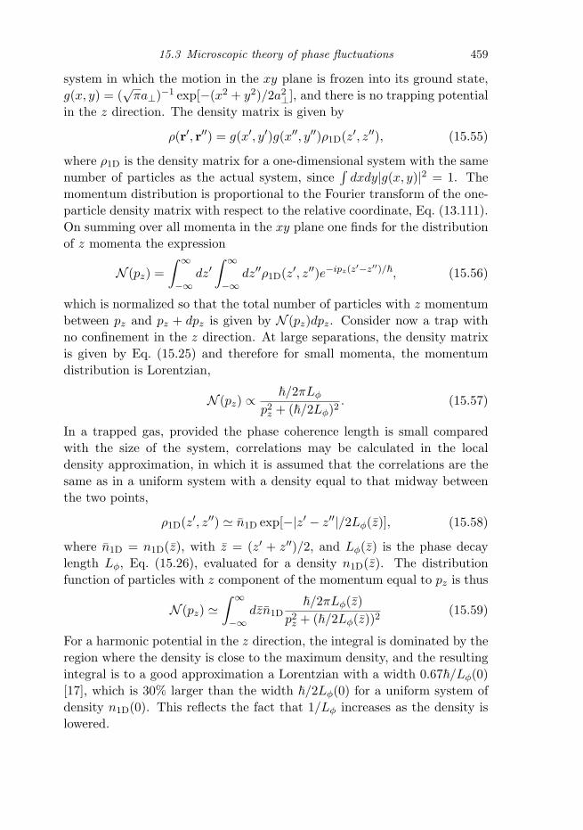
15.3 Microscopic theory of phase fluctuations 459
system in which the motion in the xy plane is frozen into its ground state,g(x, y) = (
√πa⊥)−1 exp[−(x2 + y2)/2a2
⊥], and there is no trapping potentialin the z direction. The density matrix is given by
ρ(r′, r′′) = g(x′, y′)g(x′′, y′′)ρ1D(z′, z′′), (15.55)
where ρ1D is the density matrix for a one-dimensional system with the samenumber of particles as the actual system, since
∫dxdy|g(x, y)|2 = 1. The
momentum distribution is proportional to the Fourier transform of the one-particle density matrix with respect to the relative coordinate, Eq. (13.111).On summing over all momenta in the xy plane one finds for the distributionof z momenta the expression
N (pz) =∫ ∞
−∞dz′∫ ∞
−∞dz′′ρ1D(z′, z′′)e−ipz(z′−z′′)/�, (15.56)
which is normalized so that the total number of particles with z momentumbetween pz and pz + dpz is given by N (pz)dpz. Consider now a trap withno confinement in the z direction. At large separations, the density matrixis given by Eq. (15.25) and therefore for small momenta, the momentumdistribution is Lorentzian,
N (pz) ∝�/2πLφ
p2z + (�/2Lφ)2
. (15.57)
In a trapped gas, provided the phase coherence length is small comparedwith the size of the system, correlations may be calculated in the localdensity approximation, in which it is assumed that the correlations are thesame as in a uniform system with a density equal to that midway betweenthe two points,
ρ1D(z′, z′′) � n1D exp[−|z′ − z′′|/2Lφ(z)], (15.58)
where n1D = n1D(z), with z = (z′ + z′′)/2, and Lφ(z) is the phase decaylength Lφ, Eq. (15.26), evaluated for a density n1D(z). The distributionfunction of particles with z component of the momentum equal to pz is thus
N (pz) �∫ ∞
−∞dzn1D
�/2πLφ(z)p2
z + (�/2Lφ(z))2(15.59)
For a harmonic potential in the z direction, the integral is dominated by theregion where the density is close to the maximum density, and the resultingintegral is to a good approximation a Lorentzian with a width 0.67�/Lφ(0)[17], which is 30% larger than the width �/2Lφ(0) for a uniform system ofdensity n1D(0). This reflects the fact that 1/Lφ increases as the density islowered.

460 Lower dimensions
In the experiment, the momentum distribution obtained by Bragg diffrac-tion, after expansion of the cloud, was measured as a function of detuningfor a range of temperatures and the resulting distribution was indeed foundto be Lorentzian. The width of the distribution, which is a measure of thephase correlation length, was found to agree with the theoretical expression(15.26) to within the 15% uncertainty of the experiment.
15.4 The one-dimensional Bose gas
Lower-dimensional systems play an important role in physics because thereexist exact solutions for a number of models of such systems. These provide atesting ground for approximate theoretical methods, and in addition can becompared directly with experiment. The one-dimensional uniform Bose gaswith repulsive zero-range interactions is one such example. The Hamiltonianis
H = −N∑
i=1
�2
2m
∂2
∂x2i
+N∑
i,j (i<j)
U (1)δ(xi − xj). (15.60)
Here U (1) is the two-body interaction strength, which we write as
U (1) = c�
2
m. (15.61)
The parameter c has the dimensions of an inverse length, and the quantity
γ =c
n1D(15.62)
is a dimensionless measure of the coupling strength. Here n1D = N/L,L being the length of the system. Notice that the coupling decreases asthe density increases, in contrast to the situation in three dimensions. Su-perficially, the interaction in Eq. (15.60) resembles the effective low-energyinteraction (5.34). However, the Hamiltonian (15.60) is the bare one, andthe corresponding eigenstates are the full many-body states.
Such a one-dimensional system may be experimentally realized by confin-ing the atoms to a highly elongated harmonic trap of transverse frequencyω⊥ and axial frequency ωz = λω⊥, with λ 1. We have seen that, if thescattering length is small compared with the extent of the zero-point mo-tion perpendicular to the axis, U (1) is given for a gas so dilute that binarycollisions dominate by Eq. (15.48), and therefore, with ax = ay = a⊥, onefinds c = 2a/a2
⊥.As shown by Lieb and Liniger [6], the eigenstates and eigenvalues of the
Hamiltonian (15.60) may be found by use of an ansatz for the states of the

15.4 The one-dimensional Bose gas 461
system pioneered by Bethe for the one-dimensional Heisenberg model of aferromagnetic spin chain [18]. The basic idea of the method is that themany-body wave function Ψ(x1, x2, . . . , xN ) is a solution of the free-particleSchrodinger equation except when two particles coincide. Surprisingly, themodel may be solved simply for γ → ∞, which is referred to as the Tonks–Girardeau limit [7, 8].
15.4.1 The strong-coupling limit
In the limit γ → ∞, the wave function must vanish when any two atomscoincide, otherwise the energy would grow without limit. Thus Ψ mustvanish if any two particles coincide,
Ψ|xj=xk= 0 (15.63)
for all j and k �= j. An expression which satisfies this condition and whichis a solution of the free-particle Schrodinger equation is the determinant
Ψ(x1, x2, . . . , xN )F ∝ det[eikjxl ] ≡
∣∣∣∣∣∣∣∣eik1x1 eik1x2 .. eik1xN
eik2x1 eik2x2 .. eik2xN
.. .. .. ..
eikNx1 eikNx2 .. eikNxN
∣∣∣∣∣∣∣∣. (15.64)
This wave function, a Slater determinant, is antisymmetric under inter-change of two particle coordinates, so it is appropriate for fermions. Forbosons, the wave function must be symmetric under interchange of two par-ticle coordinates, and a wave function having this symmetry is
Ψ(x1 . . . , xN ) ∝ det[eikjxl ]∏
1≤s<t≤N
sign(xt − xs), (15.65)
where sign(x) = 1 for x > 0 and sign(x) = −1 for x < 0. The wave function(15.65) satisfies (15.63) and is an eigenfunction of the Hamiltonian (15.60)with eigenvalue
E =�
2
2m
N∑j=1
k2j . (15.66)
The state is also an eigenstate of the total momentum, with eigenvalue
P = �
N∑j=1
kj . (15.67)
To get rid of end effects, one imposes a periodic boundary condition,

462 Lower dimensions
–1 –0.5 0 0.5 10
0.5
1
1.5
(x1– x
2)/L
(x1,x
2)L = 1
10 10
Fig. 15.1 Wave function for the relative motion of two bosons for different valuesof γ.
expressed by the equation
Ψ(x1, . . . , xj = 0, . . . , xN ) = Ψ(x1, . . . , xj = L, . . . , xN ), (15.68)
where L is the length of the system. For identical bosons, the symmetry ofthe wave function under interchange of particle coordinates implies that, ifthe condition holds for one value of j, it holds for all j.
We begin by finding the eigenstates of the system, assuming that theperiodicity condition (15.68) holds for a wave function of the form (15.65).Consider the dependence of Ψ on x1. This has two sources, the exponentialfactors and the sign functions. When x1 advances from zero to L, theproduct of sign-functions in (15.65) changes by a factor (−1)N−1, since N−1differences of coordinates change sign, and eikjx1 changes by a factor eikjL.Since the periodicity condition on x1 must hold for all values of x2, . . . xN ,it must apply for each of the components of the wave function proportionalto eikjx1 separately, from which it follows that
eikjL = (−1)N−1 = e−iπ(N+1). (15.69)

15.4 The one-dimensional Bose gas 463
Therefore the wave vectors may be written in the form
kj =2π
L
(nj −
N + 12
), (15.70)
with nj being an arbitrary integer. The subtracted term in Eq. (15.70)ensures that the allowed values of kj are integer multiples of 2π/L for oddN and half-odd-integer multiples for even N , and the form we have chosenmakes the description of the ground state simple, as we shall see. One couldequally well have used, e.g., (N mod 2)/2 instead of (N +1)/2, since the setof allowed wave vectors would be the same, but the correspondence betweena wave vector and an integer would be different.
The ground state is obtained by minimizing the energy expression (15.66).For the case of two particles one has k1 = −k2 = π/L and the normalizedground-state wave function is
Ψ(x1, x2) =√
2L
sin(
π|x1 − x2|L
), (15.71)
which is plotted in Fig. 15.1. In general, the ground state is obtained by theN distinct wave vectors kj that have the smallest magnitudes, namely
kj =2π
L
(j − N + 1
2
), j = 1, 2 . . . , N . (15.72)
The determinant in the ground-state wave function has the form
det[eikjxl ] = exp
{−iπ(N + 1)(
∑i
xi)/L
}det[ei2πjxl/L]
= exp
{−iπ(N − 1)(
∑i
xi)/L
}det[{ei2πxl/L}j−1]
= exp
{−iπ(N − 1)(
∑i
xi)/L
}det[ζj−1
l ], (15.73)
where ζl = ei2πxl/L. The final determinant is known as a van der Mondedeterminant, and it vanishes when ζl = ζr for l �= r, since then tworows of the determinant are the same, and therefore it must be propor-tional to
∏1≤l<r≤N (ζr − ζl). It is a polynomial of degree N(N − 1)/2
and the term made up only from elements on the diagonal is∏N
r=2(ζr)r−1,so the determinant must be equal to
∏1≤l<r≤N (ζr − ζl). Since ζr − ζl =
(ζrζl)1/22i sin{π(xr − xl)/L}, it follows that the normalized N -particleground-state wave function Ψ∞ in the Tonks–Girardeau limit (γ → ∞)

464 Lower dimensions
may be written as
Ψ∞ =2N(N−1)/2
√N !LN
∏i<j
| sin[π(xi − xj)/L]|. (15.74)
The wave function is the product of factors for each pair of particles, and ithas the form introduced by Jastrow in the many-body problem for systemswith short-range interactions [19]. However, the physics in the two casesis different, and in the one-dimensional Bose gas, in contrast to dense sys-tems like nuclear matter, the correlation factor is not of short range. Thenormalization factor follows from the fact that(
N∏l=1
∫ L
0dxl
)|det[ζj−1
l ]|2 = N !LN . (15.75)
This may be demonstrated by observing that the determinant has N ! terms.In the integral of the squared modulus, the only non-vanishing contributionscome when a term in the determinant is multiplied by its complex conjugate.Since |ζl|2 = 1, each such contribution gives a factor LN . The other con-tributions vanish because their integrands contain factors of the type (ζl)νl ,where νl is a non-zero integer, which vanish when integrated over the range0 ≤ xl ≤ L.
In the thermodynamic limit N → ∞, L → ∞ with the density n1D = N/L
being kept constant, the sum over j of a quantity G(kj) can be replaced byan integral over k according to the relation
N∑j=1
G(kj) →L
2π
∫ k0
−k0
G(k)dk, (15.76)
where
k0 =mv0
�= πn1D, (15.77)
since (15.72) shows that k is limited to the interval between −πN/L andπN/L. The momentum p0 = �k0 = mv0, with v0 given by Eq. (15.45), isthe Fermi momentum of a one-component (spinless) Fermi gas with densityn1D. Thus Eq. (15.66) gives for the ground-state energy per particle
E
N=
13
�2k2
0
2m=
π2
6�
2n21D
m, (15.78)
and the total momentum is zero. Since E is proportional to N3, the chemicalpotential μ = (∂E/∂N)L is
μ =�
2k20
2m=
π2
2�
2n21D
m. (15.79)

15.4 The one-dimensional Bose gas 465
Thermodynamic quantities such as pressure and sound velocity at zerotemperature are obtained from (15.78) by generalizing the results of Sec.10.4 to one dimension. The pressure p is thus2
p = −(
∂E
∂L
)N
=2E
L=
π2
3�
2
mn3
1D, (15.80)
while the sound velocity s is given by
s2 =1m
∂p
∂n1D=(
�k0
m
)2
= v20. (15.81)
Surprisingly, the expressions for thermodynamic quantities are exactly thesame as those for a one-component (spinless) Fermi gas of the same density.This is a consequence of a one-to-one correspondence between states of thetwo systems [8]. States of both systems are characterized by a set of N
integers, nj , none of which is repeated, and the energy is given by Eq.(15.66). For an odd number of particles, the allowed k-values for the twosystems are integer multiples of 2π/L, while for an even number of particlesthey are half-odd-integer multiples of 2π/L. In the limit of a large numberof particles, the difference between the k-values for odd and even N has noeffect on thermodynamic properties to leading order in 1/N .
However, other properties such as the momentum distribution and two-and higher-body correlation functions, are sensitive to statistics, since thewave function for the Bose problem differs from that for free fermions be-cause of the sign functions in Eq. (15.65).
The ground state is specified by the set of numbers {nj} = {1, 2, . . . , N}.An example of an excited state is given by {nj} = {1, 2, . . . , N − 1, N + λ},where λ is a positive integer. The momentum of the state is q = λ2π�/L,and its energy measured with respect to the ground-state energy is
εq =(p0 + q)2
2m− p2
0
2m=
p0
mq +
q2
2m. (15.82)
For the Bose gas, these excitations correspond to sound modes and at longwavelengths their velocity is v0 = p0/m, in agreement with the velocity ofsound calculated from thermodynamics, Eq. (15.81). In a free Fermi gas,the excitation is a particle–hole pair, the particle being outside the Fermisurface and the hole right at the Fermi surface.
Another way to create an excitation is to remove one of the integersbetween 0 and N in the ground-state set and add the integer N + 1,2 The quantity −(∂E/∂L)N has the dimensions of force, but in accord with the practice in the
literature, we shall denote it by p and refer to it as the pressure.

466 Lower dimensions
{nj} = {1, 2, . . . , N −λ, N −λ+2, . . . , N +1}. The momentum of this stateis again q = λ2π�/L and for large N the energy relative to the ground-stateenergy is
εq =p0
mq − q2
2m. (15.83)
These excitations are analogues of solitons in the dilute Bose gas. Theirgroup velocity is zero for q = p0, which corresponds to the black solitondescribed for weak coupling in Sec. 7.6.1. For the Fermi gas, the excitationsare again particle–hole pairs, the particle being right at the Fermi surfaceand the hole inside.
15.4.2 Arbitrary coupling
We shall now demonstrate how one generalizes the wave function (15.65) tothe case of arbitrary coupling. To keep the presentation simple, we first con-sider the case of two bosons and then indicate how the result is generalizedto N bosons.
The two-body problem
First let us calculate by elementary methods the wave function and ground-state energy of two identical bosons, each of mass m, interacting via a delta-function potential. The lowest energy is obtained when the centre-of-massmomentum is equal to zero, and since the interaction only depends on therelative coordinate x = x1 −x2, the wave function only depends on x. Sincethe particles are bosons, the wave function is an even function of x, and wecan therefore take it to have the form
Ψ(x) = A cos kx + B sin k|x|. (15.84)
The periodic boundary condition (15.68) for this case is Ψ(0) = Ψ(L), whichimplies that
A = A cos kL + B sin kL (15.85)
orB
A= tan(kL/2). (15.86)
The delta-function interaction gives rise to a discontinuity in the derivativeof the wave function. To see this, we express the kinetic energy operator forthe two particles in terms of the centre-of-mass coordinate X = (x1 + x2)/2

15.4 The one-dimensional Bose gas 467
and the relative coordinate x = x1 − x2. Since
∂
∂x21
+∂
∂x22
=12
∂
∂X2+ 2
∂
∂x2, (15.87)
the Schrodinger equation for the wave function Ψ(x) becomes
−�2
m
d2Ψdx2
+ U (1)δ(x)Ψ = EΨ. (15.88)
By integrating Eq. (15.88) from x = −η to x = η, where η is a positiveinfinitesimal we get
dΨdx
∣∣∣∣x=η
− dΨdx
∣∣∣∣x=−η
= cΨ(0), (15.89)
where c = mU (1)/�2. Alternatively, this condition may be expressed in
terms of the original variables, using the relation ∂/∂x = (∂/∂x1−∂/∂x2)/2:(∂
∂x1− ∂
∂x2
)Ψ|x1=x2+η −
(∂
∂x1− ∂
∂x2
)Ψ|x1=x2−η = 2cΨ|x1=x2 . (15.90)
Because the wave function is symmetric in the coordinates, the two termson the left-hand side are equal, and therefore(
∂
∂x1− ∂
∂x2
)Ψ|x1=x2+η = cΨ|x1=x2 . (15.91)
Application of condition (15.89) at x = 0 yields 2kB = cA or
B
A=
c
2k. (15.92)
The two expressions (15.86) and (15.92) for B/A provide a consistency re-lation for the wave vector k,
c = 2k tan(kL/2). (15.93)
This equation has infinitely many roots, and the one with the lowest magni-tude of k corresponds to the ground state. As c grows from zero to infinity,the lowest k-value increases from zero to π/L. For comparison with resultsfor the thermodynamic limit it is useful to express the condition (15.93) interms of the dimensionless coupling parameter γ (15.62). For the two-bodyproblem, the density (15.6) is n1D = N/L = 2/L. Therefore γ = cL/2 andEq. (15.93) becomes
γ = α tan(α/2), (15.94)
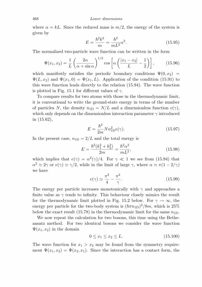
468 Lower dimensions
where α = kL. Since the reduced mass is m/2, the energy of the system isgiven by
E =�
2k2
m=
�2
mL2α2. (15.95)
The normalized two-particle wave function can be written in the form
Ψ(x1, x2) =1L
(2α
α + sinα
)1/2
cos[α
(|x1 − x2|
L− 1
2
)], (15.96)
which manifestly satisfies the periodic boundary conditions Ψ(0, x2) =Ψ(L, x2) and Ψ(x1, 0) = Ψ(x1, L). Application of the condition (15.91) tothis wave function leads directly to the relation (15.94). The wave functionis plotted in Fig. 15.1 for different values of γ.
To compare results for two atoms with those in the thermodynamic limit,it is conventional to write the ground-state energy in terms of the numberof particles N , the density n1D = N/L and a dimensionless function e(γ),which only depends on the dimensionless interaction parameter γ introducedin (15.62),
E =�
2
2mNn2
1De(γ). (15.97)
In the present case, n1D = 2/L and the total energy is
E =�
2(k21 + k2
2)2m
=�
2α2
mL2, (15.98)
which implies that e(γ) = α2(γ)/4. For γ 1 we see from (15.94) thatα2 � 2γ or e(γ) � γ/2, while in the limit of large γ, where α � π(1 − 2/γ)we have
e(γ) � π2
4− π2
γ. (15.99)
The energy per particle increases monotonically with γ and approaches afinite value as γ tends to infinity. This behaviour closely mimics the resultfor the thermodynamic limit plotted in Fig. 15.2 below. For γ → ∞, theenergy per particle for the two-body system is (�πn1D)2/8m, which is 25%below the exact result (15.78) in the thermodynamic limit for the same n1D.
We now repeat the calculation for two bosons, this time using the Bethe-ansatz method. For two identical bosons we consider the wave functionΨ(x1, x2) in the domain
0 ≤ x1 ≤ x2 ≤ L. (15.100)
The wave function for x1 > x2 may be found from the symmetry require-ment Ψ(x1, x2) = Ψ(x2, x1). Since the interaction has a contact form, the

15.4 The one-dimensional Bose gas 469
function Ψ satisfies the free-particle Schrodinger equation except where thetwo particles coincide. We therefore search for solutions of the form
ψ = Aeik1x1eik2x2 + Beik2x1eik1x2 , (x1 ≤ x2), (15.101)
where k1 and k2 are two wave vectors. The state has total momentum�(k1 + k2). To relate the coefficients A and B to each other, we use thecondition (15.91), which yields
i(k2 − k1)(A − B) = c(A + B), (15.102)
orB
A=
k2 − k1 + ic
k2 − k1 − ic. (15.103)
Thus for real k2 − k1, |B| = |A|. For c → ∞, B → −A and thereforeΨ(x1, x1) = 0, in agreement with our discussion of the Tonks–Girardeaulimit. For smaller values of c there is a phase difference between the twocomponents of the wave function given by B/A = eiα, where α = π −2 tan−1[(k2 − k1)/c]. From Eq. (15.103) it follows that the wave function inthe domain (15.100) is given by
Ψ(x1, x2) ∝ (k2 − k1 − ic)ei(k1x1+k2x2)
+(k2 − k1 + ic)ei(k2x1+k1x2). (15.104)
From the symmetry of the wave function under interchange of particle co-ordinates, we obtain the following expression for the wave function valid forall 0 ≤ x1 ≤ L and 0 ≤ x2 ≤ L:
Ψ(x1, x2) ∝ [k2 − k1 − ic sign(x2 − x1)]ei(k1x1+k2x2)
−[k1 − k2 − ic sign(x2 − x1)]ei(k2x1+k1x2). (15.105)
This wave function is an eigenfunction of the total momentum, with eigen-value �(k1 + k2), and of the Hamiltonian, with eigenvalue �
2(k21 + k2
2)/2m.The requirement that the wave function also satisfy the periodic boundarycondition Ψ(0, x2) = Ψ(L, x2) for all x2 implies that
eik1L = e−ik2L =k1 − k2 + ic
k1 − k2 − ic. (15.106)
Because of the symmetry under interchange of coordinates, the periodicitycondition Ψ(x1, 0) = Ψ(x1, L) is automatically satisfied. From Eq. (15.106)we see that the total momentum is given by
P = �(k1 + k2) = ν2π�
L, (15.107)

470 Lower dimensions
where ν is an integer. The ground state has total momentum zero, andtherefore we write k1 = −k2 = k, and the periodicity condition (15.106)then gives the result (15.93) for k previously derived from elementary con-siderations.
The many-body problem
Now we proceed to the case of N particles, which was solved by Lieb andLiniger [6]. The reader may find a complete discussion in Ref. [20]. As inthe case of two particles, one can obtain a boundary condition on the wavefunction by integrating over a relative coordinate, and it has the same formas the jump condition (15.91) for the two-body problem, except that thewave function is now a function of N coordinates.
Consider the following wave function, which is symmetric in the particlecoordinates and is a generalization of Eq. (15.65):
Ψ(x1, . . . , xN ) =
N∑P
(−1)[P ] exp(iN∑
n=1
kPnxn)∏j>l
[kPj − kPl− ic sign(xj − xl)], (15.108)
where N is a normalization factor. Here the sum extends over all permuta-tions P of the set of wave vectors k1, k2, . . . , kN , and [P ] denotes the parityof the permutation. This wave function is symmetric under interchange ofparticles, and therefore if the jump condition is satisfied for the pair of coor-dinates x1 and x2, it is satisfied for all pairs of coordinates. The componentsof the wave function (15.108) proportional to ei(kjx1+klx2) and ei(klx1+kjx2)
are given, apart from an overall multiplicative function of x3, x4, . . . , xN , by
Ψjl ∝ [kl − kj − ic sign(x2 − x1)]ei(kjx1+klx2)
−[kj − kl − ic sign(x2 − x1)]ei(klx1+kjx2). (15.109)
The difference in the sign of the two terms is due to the factor (−1)[P ] in Eq.(15.108) and the fact that the two terms differ by the interchange of kj andkl, and therefore the two permutations have opposite parities. Since thiscomponent of the N -body wave function has the same form as the two-bodywave function (15.105), it satisfies the jump condition (15.91) and thereforeΨ, which is a sum of such components, satisfies the jump condition. Thusthe wave function satisfies the N -body Schrodinger equation, and the statehas energy
E =N∑
j=1
�2k2
j
2m(15.110)

15.4 The one-dimensional Bose gas 471
and momentum
P =N∑
j=1
�kj . (15.111)
By analogy with (15.106) in the two-particle case, the periodic boundarycondition leads to the relations
exp(ikjL) =∏
l( �=j)
kj − kl + ic
kj − kl − ic, j = 1, 2, . . . , N. (15.112)
When c → ∞ these conditions reduce to (15.69). By taking the logarithmof (15.112) we obtain
kjL +N∑
l=1
θ(kj − kl) = 2π
(nj −
N + 12
)(15.113)
with
θ(k) = i ln(
ic + k
ic − k
)= 2 arctan(k/c), (15.114)
where the second form applies for real k, which is the case of interest here.We take the branch of the function corresponding to θ(k) = ±π for k → ±∞,and θ(k) is then a continuous function of k. Note that (15.113) reduces to(15.70) in the limit c → ∞. These N equations determining the wave vectorsare referred to as the Bethe equations.
We now determine the ground state, which is characterized by k-valuesthat are closest to zero. By analogy with (15.72) we get
kjL +N∑
l=1
θ(kj − kl) = 2π
(j − N + 1
2
), j = 1, 2, . . . , N. (15.115)
We consider the thermodynamic limit and therefore take the difference be-tween the equations (15.115) for j + 1 and j. Since the difference kj+1 − kj
is of order 1/L, we may replace the difference of the θ functions by the firstterm in a Taylor expansion and the result is
(kj+1 − kj)L + (kj+1 − kj)N∑
m=1
θ′(kj − km) = 2π, (15.116)
where
θ′(k) =dθ
dk=
2c
c2 + k2. (15.117)
Let us introduce the function f(k) which represents the density of states in

472 Lower dimensions
0 10 20 30 40 50 600
0.5
1
1.5
2
2.5
3
3.5
e()
0 5 100
0.5
1
e'()
Fig. 15.2 The function e(γ), which equals the ground-state energy per particle E/Ndivided by �
2n21D/2m, in the thermodynamic limit (N → ∞). The inset shows the
derivative e′(γ) = de(γ)/dγ.
k-space in the sense that Lf(k)dk is the number of states in the infinitesimalinterval dk centred at k. Then kj+1 − kj = 1/Lf(kj) and (15.116) becomes
1 + 2c
∫ K
−K
f(k′)dk′
c2 + (k − k′)2= 2πf(k). (15.118)
Here K denotes the upper limit for |k|, which is determined by the conditionthat the total number of k-values be equal to the number of particles, N ,
N = L
∫ K
−Kf(k)dk. (15.119)
The total ground-state energy E is found by integrating the single-particleenergy �
2k2/2m over k,
E =�
2
2mL
∫ K
−Kk2f(k)dk. (15.120)
By scaling the momentum variable k by the upper limit, k = Ky, and

15.4 The one-dimensional Bose gas 473
defining g(y) ≡ f(Ky) and λ ≡ c/K, one finds that the three equations(15.118)–(15.120) together with the definition (15.97) become
g(y) =12π
+λ
π
∫ 1
−1
g(t)dt
λ2 + (y − t)2, (15.121)
λ = γ
∫ 1
−1g(t)dt, (15.122)
and
e(γ) =γ3
λ3
∫ 1
−1t2g(t)dt. (15.123)
To gain insight into the solution to the inhomogeneous integral equation(15.121) let us consider the Tonks–Girardeau limit, in which γ → ∞. Sinceλ also tends to infinity in that limit (recall that n1D/K = λ/γ), the solutionto (15.121) is g = 1/2π, from which it follows according to (15.122) thatλ = γ/π. By insertion of these values into (15.123) we obtain e(∞) = π2/3,which implies that the ground-state energy per particle is given by Eq.(15.78) and the chemical potential by Eq. (15.79) obtained previously inthe Tonks–Girardeau limit. To find the correction to g to leading order inλ−1 we may replace the denominator in the integrand in Eq. (15.121) by λ2.This yields g � 1/2π + (π2λ)−1 � 1/2π + 1/πγ. The density of states thusremains constant, but it is increased because the range of k-values (2K)is reduced as the interaction becomes weaker. When the expression for g
is inserted in (15.122) one finds λ � (γ + 2)/π and therefore the energy(15.123) is given by
e(γ) � π2
3
(1 − 4
γ
). (15.124)
To leading order in 1/γ the result (15.124) is 4/3 times the result (15.99)obtained above for two bosons, e(γ) � (π2/4)(1 − 4/γ).
In the opposite limit, for γ → 0, the energy may be calculated in first-order perturbation theory, using the normalized zero-order wave function
Ψ0 =1
LN/2, (15.125)
which describes a state in which all N particles occupy the same zero-momentum single-particle state k = 0. This gives
E(1) � N�
2
2mn2
1Dγ, (γ 1). (15.126)
The integral equation (15.121) may be solved numerically for general γ, and

474 Lower dimensions
the resulting e(γ) is plotted in Fig. 15.2. From e(γ), one may determine thepressure, the chemical potential and the sound velocity, which are given by
p = −(
∂E
∂L
)N
=�
2
mn3
1D
[e(γ) − 1
2γe′(γ)
], (15.127)
μ =(
∂E
∂N
)L
=�
2
mn2
1D
[32e(γ) − 1
2γe′(γ)
], (15.128)
and
s2 =1m
∂p
∂n1D=
�2
m2n2
1D
[3e(γ) − 2γe′(γ) +
12γ2e′′(γ)
]. (15.129)
15.4.3 Correlation functions
Since we know the wave function of the ground state, one might anticipatethat calculating correlation functions would be straightforward. However,for a large number of particles, the Bethe-ansatz wave function (15.108) isvery unwieldy. In this section, we shall consider a number of properties ofcorrelations which can be obtained without the need for a frontal attack withthe full machinery of the Bethe-ansatz method. As we shall see, calculationsfor a relatively small number of particles give a good approximation to resultsfor the thermodynamic limit. We begin with the two-particle correlationfunction and then discuss the momentum distribution.
Two-particle correlation function
In Sec. 13.3 we introduced the two-particle correlation function g2, whichwas defined in terms of creation and annihilation operators in Eq. (13.82).For our present purposes it is convenient to work directly with the wavefunction. In second-quantized notation, the state of the system is
|Ψ〉 =1
(N !)1/2
(N∏
i=1
∫ L
0dxiψ
†(xi)
)Ψ(x1, x2, . . . , xN )|0〉, (15.130)
and therefore the density at point x′ is given by
<ψ†(x′)ψ(x′)> = N
∫ L
0dx2
∫ L
0dx3 . . .
∫ L
0dxN |Ψ(x′, x2, . . . , xN )|2.
(15.131)In first-quantized form, the operator for the density is
∑Ni=1 δ(x′ − xi), and
the factor of N in Eq. (15.131) reflects the N different ways of choosing

15.4 The one-dimensional Bose gas 475
which of the xi should be equal to x′. Similarly, one finds for the two-particle correlation function
g2(x′, x′′) = N(N − 1)∫ L
0dx3
∫ L
0dx4 . . .
∫ L
0dxN |Ψ(x′, x′′, x3, . . . , xN )|2.
(15.132)The prefactor may be understood by observing that in first-quantized no-tation the two-particle correlation operator is
∑i,j(i�=j) δ(x′ − xi)δ(x′′ − xj),
and there are N(N − 1) ways of choosing the pair of indices.For the systems considered in this section, the two-particle correlation
function depends only on the difference x ≡ x′ − x′′ of the two arguments.Thus, for the two-body problem, one finds from Eq. (15.96) that g2, Eq.(15.132), is given by
g2(x) = 2Ψ(x′, x′ − x)2 =4 cos2[α(1/2 − |x|/L)]
L2[1 + (sin α)/α], N = 2. (15.133)
The Bethe-ansatz wave function becomes increasingly difficult to workwith as N increases, but for zero separation, the two-particle correlationfunction may be calculated from the energy of the system by use of a resultgenerally referred to as the Hellmann–Feynman theorem, although it hasbeen attributed to others. To prove it, consider a Hamiltonian H(η) thatdepends on some parameter η, and let |η〉 be an eigenstate of the Hamilto-nian with energy E(η). Since E(η) = 〈η|H(η)|η〉 it follows that
∂E
∂η= 〈η|
(∂H
∂η
)|η〉 +
(∂〈η|∂η
)H|η〉 + 〈η|H
(∂|η〉∂η
)
= 〈η|(
∂H
∂η
)|η〉 + E
∂〈η|η〉∂η
= 〈η|(
∂H
∂η
)|η〉, (15.134)
where the last form is a consequence of the normalization condition 〈η|η〉 = 1for all η. When applied to the Hamiltonian (15.60), this gives
∂E
∂U (1)= <
N∑i,j(i<j)
δ(xi − xj)>
=∫ L
0dx <
N∑i,j(i<j)
δ(x − xi)δ(x − xj)> =L
2g2(0), (15.135)
where in writing the final form we have made use of the translational in-variance of the system, which implies that g2 depends only on the differ-ence of the two coordinates. With the use of Eq. (15.97) and the relation
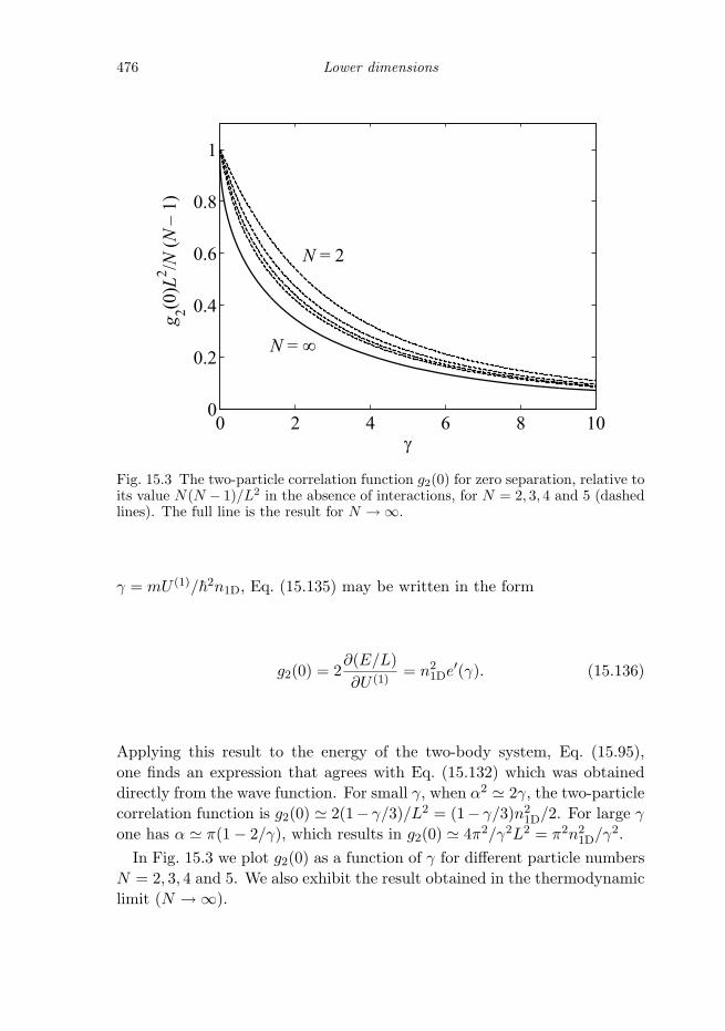
476 Lower dimensions
0 2 4 6 8 100
0.2
0.4
0.6
0.8
1g 2(0
)L2 /N
(N–
1)
N =
N = 2
Fig. 15.3 The two-particle correlation function g2(0) for zero separation, relative toits value N(N − 1)/L2 in the absence of interactions, for N = 2, 3, 4 and 5 (dashedlines). The full line is the result for N → ∞.
γ = mU (1)/�2n1D, Eq. (15.135) may be written in the form
g2(0) = 2∂(E/L)∂U (1)
= n21De′(γ). (15.136)
Applying this result to the energy of the two-body system, Eq. (15.95),one finds an expression that agrees with Eq. (15.132) which was obtaineddirectly from the wave function. For small γ, when α2 � 2γ, the two-particlecorrelation function is g2(0) � 2(1− γ/3)/L2 = (1− γ/3)n2
1D/2. For large γ
one has α � π(1 − 2/γ), which results in g2(0) � 4π2/γ2L2 = π2n21D/γ2.
In Fig. 15.3 we plot g2(0) as a function of γ for different particle numbersN = 2, 3, 4 and 5. We also exhibit the result obtained in the thermodynamiclimit (N → ∞).

15.4 The one-dimensional Bose gas 477
0 0.5 1 1.5 20
0.2
0.4
0.6
0.8
1
1.2
1.4
1.6
1.8
p/p0
n(p)
0 10 20 300
0.2
0.4
0.6
0.8
1
x/x0
(x)/
(0)
Fig. 15.4 Momentum distribution and one-particle density matrix as a function ofseparation for γ → ∞ and N → ∞. Here p0 = �k0 and x0 = 1/k0, where k0 = πn1D
(see Eq. (15.77)).
Momentum distribution
The momentum distribution is given in terms of the one-particle densitymatrix by Eq. (13.111), and here we shall consider the limiting behavioursfor small momenta and for large momenta. The one-particle density ma-trix for large separations varies as |x|−s/2v0 , Eq. (15.46), and therefore themomentum distribution for small p behaves as
n(p) ∝∫
dxe−ipx/�|x|−s/2v0 ∝ 1p1−s/2v0
. (15.137)
The sound velocity, which is given by Eq. (15.129), varies between zero andv0 as γ increases, and therefore the momentum distribution varies as 1/p
for weak coupling and 1/p1/2 in the strong-coupling Tonks–Girardeau limit.Notice that Eq. (15.137) holds even when the coupling is not weak. Many-body correlations are taken into account implicitly through the dependenceof the sound speed on coupling.
For large momenta, the momentum distribution varies as 1/p4 due tothe discontinuity in the derivative of the wave function when two particles

478 Lower dimensions
coincide [21],
n(p) � �4c2g2(0)
p4= γ2e′(γ)
(n1D�)4
p4. (15.138)
To obtain insight into this result, we write the momentum distribution(13.111) using the form (13.107) for the density matrix and find
n(p) =N
V
∫ L
0dx2 . . .
∫ L
0dxN
∣∣∣∣∫ L
0dx1e
−ipx1/�Ψ(x1, x2, . . . , xN )∣∣∣∣2
.
(15.139)In order to understand how the behaviour shown in Eq. (15.138) arises wereturn to the case of two bosons in the ground state. Because of the jumpcondition (15.91), the wave function for small particle separations is givenby
Ψ(x1, x2) � Ψ(x2, x2) (1 + c|x1 − x2|/2) . (15.140)
The Fourier transform F (p) of a function f(x) is defined by the equation
F (p) =∫ L
0dxe−ipx/�f(x). (15.141)
For a function periodic in x with period L, the relevant momenta are pν =2π�ν/L, where ν is an integer. For these momenta, the Fourier transformmay be rewritten by integrating by parts twice, which gives
F (p) = − �
p2
∫ L
0dxe−ipx/�f ′′(x), (15.142)
where a prime denotes differentiation with respect to x. Thus a discon-tinuity in the derivative of f gives rise to a delta function in f ′′ and acontribution to F (p) varying as 1/p2. The slowly varying part of f ′′ givesrise to contributions that fall off more rapidly as p → ∞.3 By using theresult g2(0) = 2|Ψ(0, 0)|2, Eq. (15.133), one can verify the result (15.138)for the case N = 2. The proof for higher values of N follows closely thatfor N = 2, except for the fact that the derivative of the wave function hasdiscontinuities whenever x1 is equal to any of the other xi.
For arbitrary values of p, the momentum distribution may be obtainedfrom the density matrix ρ(x′, x′′) given by Eq. (13.107) which in our two-particle case becomes
ρ(x′, x′′) = 2∫ L
0dx2Ψ∗(x′′, x2)Ψ(x′, x2). (15.143)
3 As an example, the two-body wave function in the strong coupling limit is proportional to| sin πx/L|, and its Fourier transform is proportional to [1 + cos(pL/�)]/[p2 − (π�/L)2].

15.4 The one-dimensional Bose gas 479
When (15.96) is inserted into this and the integrations carried out, the re-sulting density matrix is obtained as a function ρ(|x|) of the magnitude |x|of the relative coordinate x = x′ − x′′ (Problem 15.4). For small |x| theleading non-analytic term in ρ(|x|) is found to be proportional to |x|3. Sim-ilar arguments apply for the N -particle case. The momentum distributionis given by the Fourier transform of ρ(|x|), which thus behaves as 1/p4 forlarge p, as argued previously.
The momentum distribution n(p) for a Bose gas of impenetrable particlesis very different from that of a free Fermi gas. For an ideal Fermi gas, n(p)is unity if |p| < pF and zero otherwise, while for the Bose gas n(p) variessmoothly as a function of |p|, being proportional to |p|−1/2 for small valuesof p and to p−4 for large values (Fig. 15.4). The density matrix, the Fouriertransform of which is the momentum distribution function, is also shownin Fig. 15.4 as a function of the separation x = x′ − x′′. Details of thecalculation of the momentum distribution in the thermodynamic limit aswell as references to earlier work may be found in Ref. [22].
Problems
Problem 15.1 Use the expression (15.42) to estimate the magnitude andtemperature dependence of the phase fluctuations in a three-dimensional su-perfluid of volume V at low temperatures, where the elementary excitationscan be taken to be sound waves (kT ms2).
Problem 15.2 Consider scattering of a particle of momentum �k andmass m in one dimension from a potential U (1)δ(x). For an incident waveeikx, show that the amplitude of the transmitted wave is (R0 + 1)/2 andthat of the reflected wave is (R0 − 1)/2, where R0 = −(c + ik)/(c− ik) withc = mU (1)/�
2.
Problem 15.3 Solve the Lippmann–Schwinger equation (5.45) for scat-tering in two dimensions, for a repulsive interaction of range d as a functionof the energy of the pair of particles. Show that for low energy E in thecentre-of-mass frame, the T matrix is proportional to (�2/m)/ ln(Ec/E),where Ec = �
2/md2, and determine the prefactor.
Problem 15.4 Calculate the density matrix ρ(x′, x′′), Eq. (15.143), fortwo bosons in one dimension interacting via a contact interaction as a func-tion of the separation x = x′ − x′′, where the wave function is given in Eq.(15.96). Verify the expression (15.138) for the momentum distribution atlarge momenta. Compare the momentum distribution for γ → ∞ with theresult in the thermodynamic limit plotted in Fig. 15.4.

480 Lower dimensions
References[1] D. S. Petrov, D. M. Gangardt, and G. V. Shlyapnikov, J. Phys. IV France
116, 5 (2004).[2] A. Gorlitz, J. M. Vogels, A. E. Leanhardt, C. Raman, T. L. Gustavson, J. R.
Abo-Shaeer, A. P. Chikkatur, S. Gupta, S. Inouye, T. Rosenband, and W.Ketterle, Phys. Rev. Lett. 87, 130402 (2001).
[3] H. Moritz, T. Stoferle, M. Kohl, and T. Esslinger, Phys. Rev. Lett. 91,250402 (2003).
[4] V. L. Berezinskii, Zh. Eksp. Teor. Fiz. 61, 1144 (1971) [Sov. Phys.– JETP32, 493 (1971)].
[5] J. M. Kosterlitz and D. J. Thouless, J. Phys. C. 6, 1181 (1973).[6] E. H. Lieb and W. Liniger, Phys. Rev. 130, 1605 (1963).[7] L. Tonks, Phys. Rev. 50, 955 (1936).[8] M. Girardeau, J. Math. Phys. 1, 516 (1960).[9] P. Nozieres and D. Pines, The Theory of Quantum Liquids, Vol. II,
Superfluid Bose Liquids, (Redwood City, Addison-Wesley, 1990), Chapter 6.[10] D. R. Nelson, Defects and Geometry in Condensed Matter Physics,
(Cambridge, Cambridge University Press, 2002), Chapter 6.[11] Z. Hadzibabic, P. Kruger, M. Cheneau, B. Battelier, and J. Dalibard, Nature
441, 1118 (2006).[12] D. S. Petrov, G. V. Shlyapnikov, and J. T. M. Walraven, Phys. Rev. Lett. 87,
050404 (2001).[13] M. Olshanii, Phys. Rev. Lett. 81, 938 (1998).[14] T.-L. Ho and M. Ma, J. Low Temp. Phys. 115, 61 (1999).[15] S. Dettmer, D. Hellweg, P. Ryytty, J. J. Arlt, W. Ertmer, K. Sengstock, D.
S. Petrov, G. V. Shlyapnikov, H. Kreutzmann, L. Santos, and M. Lewenstein,Phys. Rev. Lett. 87, 160406 (2001).
[16] S. Richard, F. Gerbier, J. H. Thywissen, M. Hugbart, P. Bouyer, and A.Aspect, Phys. Rev. Lett. 91, 010405 (2003).
[17] F. Gerbier, J. H. Thywissen, S. Richard, M. Hugbart, P. Bouyer, and A.Aspect. Phys. Rev. A 67, 051602 (2003).
[18] H. Bethe, Z. Phys. 71, 205 (1931).[19] R. Jastrow, Phys. Rev. 98, 1479 (1955).[20] V. E. Korepin, N. M. Bogoliubov, and A. G. Izergin, Quantum Inverse
Scattering Method and Correlation Functions (Cambridge, CambridgeUniversity Press, 1993).
[21] M. Olshanii and V. Dunjko, Phys. Rev. Lett. 91, 090401 (2003).[22] V. V. Cheianov, H. Smith, and M. B. Zvonarev, Phys. Rev. A 71, 033610
(2005).

16
Fermions
The laser cooling mechanisms described in Chapter 4 operate irrespectiveof the statistics of the atom, and they can therefore be used to cool Fermispecies. The statistics of a neutral atom is determined by the number ofneutrons in the nucleus, which must be odd for a fermionic atom. Sincealkali atoms have odd atomic number Z, their fermionic isotopes have evenmass number A. Such isotopes are relatively less abundant than those withodd A since they have both an unpaired neutron and an unpaired proton,which increases their energy by virtue of the odd–even effect. In early ex-periments, 40K [1] and 6Li atoms [2] were cooled to about one-quarter of theFermi temperature. More recently, fermionic alkali atoms have been cooledto temperatures well below one-tenth of their Fermi temperature, and inaddition a degenerate gas of the fermionic species 173Yb (with I = 5/2) hasbeen prepared [3].
In the classical limit, at low densities and/or high temperatures, clouds offermions and bosons behave alike. The factor governing the importance ofquantum degeneracy is the phase-space density introduced in Eq. (2.24),and in the classical limit 1. When becomes comparable with unity,gases become degenerate: bosons condense in the lowest single-particle state,while fermions tend towards a state with a filled Fermi sea. As one wouldexpect on dimensional grounds, the degeneracy temperature for fermions –the Fermi temperature TF – is given by the same expression as the Bose–Einstein transition temperature for bosons, apart from a numerical factorof order unity.
As we described in Chapter 4, laser cooling alone is insufficient to achievedegeneracy in dilute gases, and it must be followed by evaporative cool-ing. The elastic collision rate, which governs the effectiveness of evaporativecooling, behaves differently for fermions and bosons when gases become de-generate. For identical fermions, the requirement of antisymmetry of the
481

482 Fermions
wave function forces the scattering cross section to vanish at low energy(see Eq. (5.24)), and therefore evaporative cooling with a single species offermion, with all atoms in the same internal state, cannot work. This dif-ficulty may be overcome by using a mixture of two types of atoms, eithertwo different fermions, which could be different hyperfine states of the samefermionic isotope, or a boson and a fermion. In the experiments on 40K,the two species were the two hyperfine states |9/2, 9/2〉 and |9/2, 7/2〉 of theatom [1], and both species were evaporated. In the lithium experiments [2],the second component was the boson 7Li. The 6Li atoms were cooled bycollisions with 7Li atoms which were cooled evaporatively, a process referredto as sympathetic cooling.
The rate of collisions is influenced not only by the statistics of the atoms,but also by the degree of degeneracy. Due to stimulated emission, degeneracyincreases collision rates for bosons. This is expressed by factors 1 + fp′ forfinal states in the expressions for rates of processes. For fermions the sign ofthe effect is opposite, since the corresponding factors are 1−fp′ , which showsthat transitions to occupied final states are blocked by the Pauli exclusionprinciple. Consequently, it becomes increasingly difficult to cool fermionsby evaporation or by collisions with a second component when the fermionsbecome degenerate.
In this chapter we describe selected topics in the physics of trappedFermi gases. We begin with equilibrium properties of a trapped gas ofnon-interacting fermions in Sec. 16.1. We then consider interactions, and inSec. 16.2 we demonstrate that generally they have little effect on static anddynamic properties provided the interaction energy per particle is small com-pared with the Fermi energy, which is the case we consider in this chapter.However, an important example where weak interactions have a large effect isa mixture of two sorts of fermion with an attractive interaction between thetwo species. Such a gas undergoes a transition to a superfluid phase similarto that for electrons in metallic superconductors. We calculate in Sec. 16.3the transition temperature to the superfluid phase and the gap in the exci-tation spectrum for equal populations of the two species, and in Sec. 16.4 weconsider the case of unequal populations. Section 16.5 deals with mixturesof bosons and fermions, and we discuss the interaction between fermions me-diated by excitations in the boson gas. In Chapter 17, we shall consider thecase of strong interatomic interactions, which can be induced by Feshbachresonances, and demonstrate the close connection between superfluidity ina Fermi gas and Bose–Einstein condensation of molecules consisting of twofermions.

16.1 Equilibrium properties 483
16.1 Equilibrium properties
We begin by considering N fermions in the same internal state. The kineticenergy due to the Fermi motion which results from the requirement thatno two particles occupy any single-particle state gives a major contributionto the total energy. Interactions are essentially absent at low temperaturebecause there is no s-wave scattering for two fermions in the same inter-nal state. This is in marked contrast to a Bose–Einstein condensate, forwhich the interaction energy dominates the kinetic energy under most ex-perimental conditions. A good first approximation to the properties of aone-component Fermi gas may therefore be obtained by treating the parti-cles as non-interacting [4].
In Sec. 2.1.1 we introduced the function G(ε), the number of states withenergy less than ε. In the ground state of the system all states with energyless than the zero-temperature chemical potential are occupied, while thosewith higher energy are empty. Since each state can accommodate only oneparticle we have
G(μ) = N, (16.1)
where μ denotes the zero-temperature chemical potential. For a power-lawdensity of states, g(ε) = Cαεα−1, the relation (16.1) yields
g(μ) =αN
μ. (16.2)
For a particle in a box (α = 3/2), the total number of states with energyless than ε is given by Eq. (2.3), G(ε) = V (2mε)3/2/6π2
�3. According
to (16.1) the Fermi energy, which equals the chemical potential at zerotemperature, and the particle number are therefore related by the condition
V(2mεF)3/2
6π2�3= N, (16.3)
and the Fermi temperature TF = εF/k is given by
kTF =(6π2)2/3
2�
2
mn2/3 ≈ 7.596
�2
mn2/3. (16.4)
The density of states g(ε) is given by Eq. (2.5). We introduce the density ofstates per unit volume by N(ε) = g(ε)/V , which is
N(ε) =g(ε)V
=m3/2ε1/2
√2π2�3
, (16.5)

484 Fermions
and therefore at the Fermi energy it is
N(εF) =g(εF)
V=
3n
2εF, (16.6)
in agreement with the general relation (16.2).For a three-dimensional harmonic trap, the total number of states with
energy less than ε is given by Eq. (2.9),
G(ε) =16
( ε
�ω
)3, (16.7)
where ω3 = ωxωyωz, and from (16.1) we then obtain the chemical potentialμ and the corresponding Fermi temperature TF as
μ = kTF = (6N)1/3�ω. (16.8)
A very good approximation for the density distribution of a trapped cloudof fermions in its ground state may be obtained by use of the Thomas–Fermi approximation, which we applied to bosons in Sec. 6.2.2. Accordingto this semi-classical approximation, the properties of the gas at a point rare assumed to be those of a uniform gas having a density equal to the localdensity n(r). The Fermi wave number kF(r) is related to the density by therelation for a homogeneous gas,
n(r) =k3
F(r)6π2
, (16.9)
and the local Fermi energy εF(r) is given by
εF(r) =�
2k2F(r)
2m. (16.10)
The condition for equilibrium is that the energy required to add a particleat any point inside the cloud be the same everywhere. This energy is thesum of the local Fermi energy and the potential energy due to the trap, andit is equal to the chemical potential of the system,
�2k2
F(r)2m
+ V (r) = μ. (16.11)
Note that the chemical potential is equal to the value of the local Fermienergy in the centre of the cloud, μ = εF(0), if one adopts the conventionthat V (0) = 0. The density profile corresponding to (16.11) is thus
n(r) =1
6π2
{2m
�2[μ − V (r)]
}3/2
, (16.12)
if V (r) < μ and zero otherwise. In a cloud of fermions the density profile

16.1 Equilibrium properties 485
is therefore more concentrated towards the centre than it is for a cloud ofbosons, for which the density varies as μ−V (r) (Eq. (6.31)). The boundaryof the cloud is determined by the condition V (r) = μ. Therefore for ananisotropic harmonic-oscillator potential of the form (2.7) the cloud extendsto distances Rx, Ry and Rz along the three axes of the trap, where
R2i =
2μ
mω2i
, i = x, y, z, (16.13)
and in general the cloud is aspherical.As a measure of the linear dimensions of the cloud we use R =
(RxRyRz)1/3, the harmonic mean of the Ri. This may be estimated from(16.8) and (16.13) to be
R = 481/6N1/6a ≈ 1.906N1/6a, (16.14)
where a = (�/mω)1/2. By contrast, the size of a cloud of bosons dependson the strength of the interaction, and ranges from a for Na/a 1 toapproximately 151/5(Na/a)1/5a for Na/a 1. For typical trap parametersand scattering lengths, a cloud of fermions is therefore generally a few timeslarger than one with the same number of bosons.
The total number of particles is obtained by integrating the density overthe volume of the cloud, and one finds
N =π2
8n(0)R3, (16.15)
or
n(0) =8π2
N
R3, (16.16)
where n(0) is the density at the centre of the cloud. Thus
kF(0) =(48N)1/3
R= 481/6 N1/6
a≈ 1.906
N1/6
a, (16.17)
which shows that the maximum wave number is of order the average inverseinterparticle separation, as in a homogeneous gas. The momentum distri-bution is isotropic as a consequence of the isotropy in momentum space ofthe single-particle kinetic energy p2/2m (Problem 16.1).
The Thomas–Fermi approximation for equilibrium properties of cloudsof fermions is valid provided the Fermi wavelength is small compared withthe dimensions of the cloud, or kF(0)Ri ∼ N1/3 1. This condition isgenerally less restrictive than the corresponding one for bosons, Na/a 1.The Thomas–Fermi approximation fails at the surface, and it is left as aproblem to evaluate the thickness of this region (Problem 16.2).

486 Fermions
We turn now to thermodynamic properties. The distribution function isgiven by the Fermi function1
f =1
e(ε−μ)/kT + 1, (16.18)
and the chemical potential μ depends on temperature. The total energy E
is therefore given by
E(T ) =∫ ∞
0dεεg(ε)f(ε), (16.19)
where g(ε) is the single-particle density of states. We again consider power-law densities of states g(ε) = Cαεα−1. At zero temperature the distributionfunction reduces to a step function, and one finds E(0) = [α/(α + 1)]Nμ.Therefore for fermions in a three-dimensional harmonic trap
E(0) =34Nμ, (16.20)
while for particles in a box (α = 3/2)
E(0) =35Nμ. (16.21)
Properties of the system at temperatures less than the Fermi tempera-ture may be estimated by carrying out a low-temperature expansion in thestandard way. For the energy one finds the well-known result
E � E(0) +π2
6g(μ)(kT )2, (16.22)
where μ is the zero-temperature chemical potential, given by Eq. (16.1).For temperatures high compared with the Fermi temperature one may cal-
culate thermodynamic properties by making high-temperature expansions,as we did for bosons in Sec. 2.4.2. The energy E tends towards its classicalvalue αNkT , as it does for bosons, and the first correction due to degeneracyhas the same magnitude as that for bosons, but the opposite sign.
16.2 Effects of interactions
As we have argued above, interactions have essentially no effect on low-temperature properties of dilute Fermi systems if all particles are in thesame internal state. However, they can play a role for a mixture of twokinds of fermions, as we shall see in more detail in Chapter 17. Consider as1 In this chapter all distribution functions are equilibrium ones, so we shall denote them by f
rather than f0.

16.2 Effects of interactions 487
an example a uniform gas containing equal densities of two kinds of fermions,which we assume to have the same mass. The kinetic energy per particleis of order the Fermi energy εF = (�kF)2/2m. The interaction energy perparticle is of order nU0, where n is the particle density for one componentand U0 = 4π�
2a/m is the effective interaction between two unlike fermions,a being the corresponding scattering length. Since the density is given byn = k3
F/6π2, the ratio of the interaction energy to the Fermi energy is
nU0
εF=
43π
kFa, (16.23)
which is of order the scattering length divided by the interparticle spacing.This is typically ∼ 10−2. For two 6Li atoms in a triplet electronic statethe scattering length is negative and exceptionally large in magnitude, andthe ratio can be of order 10−1 in zero magnetic field, but near Feshbachresonances the ratio may be of order unity or even larger. An equivalentdimensionless measure of the coupling strength is N(εF)U0 = 3nU0/2εF. Fortrapped clouds, the Fermi wave number is of order N1/6/a, and thereforethe ratio of the interaction energy to the Fermi energy is of order N1/6a/a.This dimensionless quantity is familiar from Sec. 11.1, where it was shownto give the ratio of interaction energy to kinetic energy for a Bose gas at atemperature of order Tc. The fact that it determines the ratio of these twoenergies also for Fermi systems at low temperatures reflects the similaritybetween the momentum distribution for a Bose gas near Tc and that for aFermi gas at or below the Fermi temperature. We therefore expect particleinteractions to have little influence on thermodynamic properties of trappedclouds of fermions, except when the magnitude of the scattering length iscomparable to or larger than the interparticle separation.
Equilibrium size and collective modes
Let us first consider the equilibrium size of a cloud of fermions in a harmonictrap. For simplicity, we neglect the anisotropy of the potential and take itto be of the form V (r) = mω2
0r2/2. If the spatial extent of the cloud
is ∼ R, the potential energy per particle is of order mω20R
2/2, while thekinetic energy per particle is of order N2/3
�2/2mR2, according to (16.10)
and (16.17). Observe that this is a factor N2/3 larger than the kinetic energyper particle ∼ �
2/2mR2 for a cloud of condensed bosons of the same size.In the absence of interactions the total energy thus varies as N2/3/R2 atsmall radii and as R2 at large radii, with a minimum when R is of orderN1/6(�/mω0)1/2 = N1/6aosc, in agreement with (16.14).

488 Fermions
Let us now consider the effect of interactions. If the cloud contains anequal number N of each of two fermion species, the interaction energy perparticle is of order U0N/R3. As discussed for bosons in Sec. 6.2, interactionsshift the equilibrium size of the cloud, tending to increase it for repulsiveinteractions and reduce it for attractive ones. For fermions the shift isgenerally small, since the ratio of the interaction energy to the kinetic energyis of order N1/6a/aosc, as argued above. From these considerations it isnatural to expect that interactions will have little effect on collective modes.This may be demonstrated explicitly by calculating the frequency of thebreathing mode of a cloud containing equal numbers of two different fermionspecies of equal mass in an isotropic harmonic trap. The method of collectivecoordinates described in Sec. 7.3.3 may be applied to fermions if one works interms of the density distribution rather than the condensate wave function.We parametrize the density distribution n(r) for a single species as
n(r) =CN
R3h(r/R), (16.24)
where C, a pure number, is a normalization constant. The quantity cor-responding to the zero-point energy Ezp given in (7.97) is the kinetic en-ergy due to the Pauli exclusion principle, which we may estimate using theThomas–Fermi approximation. The energy per particle for a free Fermi gasscales as the Fermi energy, which varies as n2/3, and therefore the contri-bution to the total energy scales as R−2, just as does the kinetic energyof a condensed cloud of bosons. The calculation of the frequency of thebreathing mode goes through as before, with the kinetic energy due to thePauli principle replacing the zero-point energy. The expression (7.113) forthe frequency of the monopole mode does not contain the zero-point energyexplicitly, and it is therefore also valid for clouds of fermions:
ω2 = 4ω20
[1 +
38
Eint(R0)Eosc(R0)
]. (16.25)
This result was earlier derived from sum rules in Ref. [5].The ratio Eint/Eosc is easily calculated within the Thomas–Fermi approx-
imation, for which the density profile is given by (16.12), since
Eint = U0
∫drn2(r), (16.26)
the density of each species being n(r). The energy due to the trap is
Eosc = mω20
∫drr2n(r). (16.27)

16.3 Superfluidity 489
Apart from a numerical constant, the ratio of the two energies is equal ton(0)U0/mω2
0R2 ∼ N1/6a/aosc. Thus
ω2 = 4ω20
(1 + c1N
1/6 a
aosc
), (16.28)
where c1 is a numerical constant to be determined in Problem 16.5. Theresult (16.28) shows that interactions have little effect on mode frequencieswhen N1/6|a| aosc.
According to Eq. (16.28), frequencies of collective modes in a trap dependlinearly on the interaction strength for N1/6|a| aosc. This is to be con-trasted with the situation for homogeneous gases, where a weak repulsiveinteraction between two species of fermions (say, spin-up and spin-down)of the same density gives rise to the zero-sound mode. For weak coupling,the velocity of zero sound differs from the Fermi velocity vF = pF/m by anamount proportional to vF exp[−1/N(εF)U0], which is exponentially small.Here N(εF) is the density of states (for one species) per unit volume at theFermi energy. The reason for this qualitative difference is that the strongdegeneracy of the frequencies for single-particle motion in a harmonic trapleads to larger collective effects.
16.3 Superfluidity
While the effects of particle interactions are generally small, they can bedramatic if the effective interaction is attractive. The gas is then predictedto undergo a transition to a superfluid state in which atoms are paired in thesame way as electrons are in superconducting metals. The basic theory ofthe state was developed by Bardeen, Cooper, and Schrieffer (BCS) [6], and ithas been applied widely to atomic nuclei and liquid 3He as well as to metallicsuperconductors. It was used to estimate the transition temperature of adilute Fermi gas in Ref. [7] and applied to atomic vapours in Ref. [8].
The properties of mixtures of dilute Fermi gases with attractive inter-actions are of interest in a number of contexts other than that of atomicvapours. One of these is in nuclear physics and astrophysics, where dilutemixtures of different sorts of fermions (neutrons and protons with two spinstates each) are encountered in the outer parts of atomic nuclei and in thecrusts of neutron stars. Another, to be discussed in the next chapter, isin addressing the question of how, as the strength of an attractive interac-tion is increased, the properties of a Fermi system change from those of aBCS superfluid for weak coupling to those of a system of diatomic (bosonic)molecules.

490 Fermions
A rough estimate of the transition temperature may be obtained by usinga simplified model, in which one assumes the interaction between fermionsto be a constant −|U | for states with energies within Ec of the Fermi energy,and zero otherwise. The transition temperature is predicted to be given inorder of magnitude by
kTc ∼ Ece−1/N(εF)|U |. (16.29)
For electrons in metals, the attractive interaction is a consequence of ex-change of phonons, and the cut-off energy Ec is comparable with the maxi-mum energy of an acoustic phonon �ωD, where ωD is the Debye frequency.In dilute gases, the dominant part of the interaction is the direct interactionbetween atoms. For the effective interaction between particles at the Fermisurface we take the usual low-energy result, U = U0. Since, generally, theinteraction between atoms is not strongly dependent on energy, we take thecut-off to be the energy scale over which the density of states varies, namelyεF. This leads to the estimate
kTc ∼ εFe−1/N(εF)|U0|. (16.30)
Later we shall confirm this result and evaluate the numerical coefficient.The dimensionless interaction strength λ = N(εF)|U0| at the centre of a
harmonic trap may be written as
λ = N(εF)|U0| =2π
kF(0)|a| ≈ 1.214N1/6|a|
a. (16.31)
When N1/6|a| is much less than a, λ is small, and estimated transitiontemperatures are then much less than the Fermi temperature.
In the remaining part of this section we describe the quantitative theoryof the condensed state. We first calculate the transition temperature. Fortwo-body scattering in vacuo, the existence of a bound state gives rise to adivergence in the T matrix at the energy of the state. For example, a large,positive scattering length indicates that there is a bound state at a smallnegative energy. Similarly, for two particles in a medium, the onset of pairingis signalled by a divergence in the two-body scattering, as shown by Thou-less [9], and we calculate the transition temperature by determining whenthe scattering of two fermions in the medium becomes singular. Followingthat, we describe how to generalize Bogoliubov’s method for bosons to thecondensed state of fermions. Subsequently, we demonstrate how inducedinteractions affect estimates of properties of the condensed state.

16.3 Superfluidity 491
16.3.1 Transition temperature
To understand the origin of the pairing phenomenon we investigate the scat-tering of two fermions in a uniform Fermi gas. In Sec. 5.2.1 we studied scat-tering of two particles in vacuo, and we now extend this treatment to takeinto account the effects of other fermions. Since there is no scattering atlow energies for fermions in the same internal state, we consider a mixtureof two kinds of fermions, which we denote by ‘a’ and ‘b’. As described inthe introduction to this chapter, the two fermions may be different internalstates of the same isotope. For simplicity, we shall assume that the twospecies have the same mass, and that their densities are equal. We shalldenote the common Fermi wave number by kF.
The medium has a number of effects on the scattering process. One is thatthe energies of particles are shifted by the mean field of the other particles.In a dilute gas, this effect is independent of the momentum of a particle.Consequently, the equation for the T matrix will be unaltered, provided thatenergies are measured relative to the mean-field energy of the two incomingparticles. A second effect is that some states are occupied and therefore,because of the Pauli exclusion principle, unavailable as intermediate statesin the scattering process. In the Lippmann–Schwinger equation (5.45) theintermediate state contains an a-particle with momentum p′′ and a b-particlewith momentum −p′′. This process is represented diagrammatically in Fig.16.1(a). The probabilities that these states are unoccupied are 1 − fp′′ and1−f−p′′ , and therefore the contribution from these intermediate states mustinclude the blocking factors. They are the analogues of the factors 1+f thatenhance rates of processes for bosons. Generally the distribution functionsfor the two species are different, but for the situation we have chosen they arethe same, and therefore we omit species labels on the distribution functions.Modifying the Lippmann–Schwinger equation in this way gives
T (p′,p; E) = U(p′,p) +1V
∑p′′
U(p′,p′′)(1 − fp′′)(1 − f−p′′)
E − 2ε0p′′ + iδT (p′′,p; E).
(16.32)Here ε0p = p2/2m is the free-particle energy, and we work in terms of particlemomenta, rather than wave vectors as we did in Sec. 5.2.1.
A third effect of the medium is that interactions between particles can ini-tially excite two fermions from states in the Fermi sea to states outside, or,in other words, two particles and two holes are created. The two holes thenannihilate with the two incoming particles. This process is represented inFig. 16.1(b). The contribution to the Lippmann–Schwinger equation fromthis process differs from that for two-particle intermediate states in two
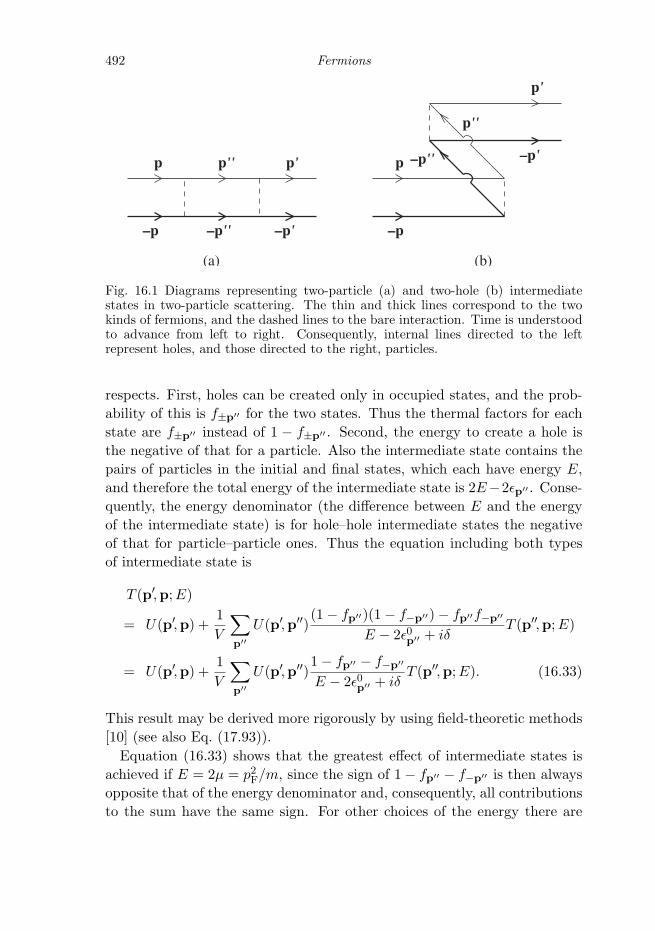
492 Fermions
–p –p'' –p'
p'p''
p''
p
–p
p –p'' –p'
p'
(a) (b)
Fig. 16.1 Diagrams representing two-particle (a) and two-hole (b) intermediatestates in two-particle scattering. The thin and thick lines correspond to the twokinds of fermions, and the dashed lines to the bare interaction. Time is understoodto advance from left to right. Consequently, internal lines directed to the leftrepresent holes, and those directed to the right, particles.
respects. First, holes can be created only in occupied states, and the prob-ability of this is f±p′′ for the two states. Thus the thermal factors for eachstate are f±p′′ instead of 1 − f±p′′ . Second, the energy to create a hole isthe negative of that for a particle. Also the intermediate state contains thepairs of particles in the initial and final states, which each have energy E,and therefore the total energy of the intermediate state is 2E−2εp′′ . Conse-quently, the energy denominator (the difference between E and the energyof the intermediate state) is for hole–hole intermediate states the negativeof that for particle–particle ones. Thus the equation including both typesof intermediate state is
T (p′,p; E)
= U(p′,p) +1V
∑p′′
U(p′,p′′)(1 − fp′′)(1 − f−p′′) − fp′′f−p′′
E − 2ε0p′′ + iδT (p′′,p; E)
= U(p′,p) +1V
∑p′′
U(p′,p′′)1 − fp′′ − f−p′′
E − 2ε0p′′ + iδT (p′′,p; E). (16.33)
This result may be derived more rigorously by using field-theoretic methods[10] (see also Eq. (17.93)).
Equation (16.33) shows that the greatest effect of intermediate states isachieved if E = 2μ = p2
F/m, since the sign of 1 − fp′′ − f−p′′ is then alwaysopposite that of the energy denominator and, consequently, all contributionsto the sum have the same sign. For other choices of the energy there are

16.3 Superfluidity 493
contributions of both signs, and some cancellation occurs. In future we shalltherefore put the energy E equal to 2μ.
When the T matrix diverges, the first term on the right-hand side of Eq.(16.33) may be neglected, and one finds
T (p′,p; 2μ) = − 1V
∑p′′
U(p′,p′′)1 − 2fp′′
2ξp′′T (p′′,p; 2μ), (16.34)
where ξp = p2/2m−μ. It is no longer necessary to include the infinitesimalimaginary part since the numerator vanishes at the Fermi surface. Theright-hand side depends on temperature through the Fermi function thatoccurs there, and this equation determines the temperature at which thescattering diverges.
Eliminating the bare interaction
Atomic potentials are generally strong, and they have appreciable matrixelements for transitions to states at energies much greater than the Fermienergy. If one replaces the bare interaction by a constant, the sum onthe right-hand side of Eq. (16.34) for momenta less than some cut-off, pc,diverges as pc → ∞. To remove this dependence on the high momentumstates we eliminate the bare potential in favour of U0, as was done in ourdiscussion for bosons. We write Eq. (16.34) formally as
T = UGMT, (16.35)
where GM is the propagator for two particles, the subscript indicating thatit applies to the medium. The T matrix in free space and for energy E = 0,which we here denote by T0, is given by
T0(p′,p; 0) = U(p′,p) − 1V
∑p′′
U(p′,p′′)1
2ε0p′′ − iδT0(p′′,p; 0), (16.36)
which we write formally as
T0 = U + UG0T0, (16.37)
where G0 corresponds to propagation of two free particles in vacuo. Theinfinitesimal imaginary part takes into account real scattering to intermedi-ate states having the same energy as the initial state. It gives contributionsproportional to the density of states, which varies as pF. These are smallat low densities. Thus we shall neglect them and interpret integrals asprincipal-value ones. Solving for U , we find
U = T0(1 + G0T0)−1 = (1 + T0G0)−1T0, (16.38)

494 Fermions
where the second form follows from using an identity similar to that used inderiving Eq. (5.127).
Equation (16.35) may therefore be rewritten as
T = (1 + T0G0)−1T0GMT. (16.39)
Multiplying on the left by 1 + T0G0 one finds
T = T0(GM − G0)T, (16.40)
or
T (p′,p; 2μ) =1V
∑p′′
T0(p′,p′′; 0)
[2fp′′ − 1
2ξp′′+
12ε0p′′
]T (p′′,p; 2μ). (16.41)
The quantity inside the square bracket is appreciable only for momentaless than or of the order of the Fermi momentum. This is because con-tributions from high-momentum states have now been incorporated in theeffective interaction. We may therefore replace T0 by its value for zero en-ergy and zero momentum, U0 = 4π�
2a/m. Consequently T also dependsweakly on momentum for momenta of order pF, and Eq. (16.41) reduces to
U0
V
∑p′′
[2fp′′ − 1
2ξp′′+
12ε0p′′
]= U0
∫ ∞
0dεN(ε)
(f(ε)ε − μ
− 12(ε − μ)
+12ε
)= 1,
(16.42)where f(ε) = {exp[(ε − μ)/kT ] + 1}−1 and N(ε) is the density of states perunit volume for a single species, which is given by (16.5). Since the chemicalpotential μ is here taken to be positive2 the integration over ε should beunderstood as a principal value integration. Since for positive μ we have∫ ∞
0dεε1/2
(− 1
ε − μ+
1ε
)= 0, (16.43)
the equation (16.42) becomes
U0
∫ ∞
0dεN(ε)
f(ε)ε − μ
= 1. (16.44)
In the following we solve this equation for an attractive interaction (U0 < 0)in the limit N(εF)|U0| 1, which is referred to as the weak-coupling limit.
2 The chemical potential can be negative if interactions are strong (see Sec. 17.3.3).

16.3 Superfluidity 495
Analytical results
At zero temperature the integral in (16.44) diverges logarithmically as ε → μ,and at non-zero temperatures it is cut off by the Fermi function at |ξp| ∼ kT .Thus for an attractive interaction (U0 < 0) there is always a temperatureTc at which Eq. (16.44) is satisfied. Setting T = Tc and introducing thedimensionless variables x = ε/μ and y = μ/kTc, we may write Eq. (16.44)as
1N(εF)|U0|
= −∫ ∞
0dx
x1/2
x − 11
e(x−1)y + 1. (16.45)
For weak coupling, the transition temperature is small compared with theFermi temperature, so we now evaluate the integral in (16.45) at low tem-peratures, kTc μ, which implies that μ � εF. We rewrite the integrandusing the identity
x1/2
x − 1=
1x1/2 + 1
+1
x − 1. (16.46)
The first term in (16.46) has no singularity at the Fermi surface in the limitof zero temperature, and the integral containing it may be replaced by itsvalue at zero temperature (y → ∞), which is∫ 1
0
dx
x1/2 + 1= 2(1 − ln 2). (16.47)
The integrand involving the second term in Eq. (16.46) has a singularity atthe Fermi surface, and the integral must be interpreted as a principal valueone. We divide the range of integration into two parts, one from 0 to 1− δ,and the second from 1 + δ to infinity, where δ is a small quantity which weallow to tend to zero in the end. Integrating by parts and allowing the lowerlimit of integration to tend to −∞ since Tc TF, we find∫ ∞
0
dx
x − 11
e(x−1)y + 1=∫ ∞
0dz ln(z/y)
12 cosh2 z/2
= − ln2γy
π. (16.48)
Here γ = eC ≈ 1.781, where C is Euler’s constant. By adding the contribu-tions (16.47) and (16.48) one finds that the transition temperature is givenby [7]
kTc =8γ
πe2εFe−1/N(εF)|U0| ≈ 0.61εFe−1/N(εF)|U0|. (16.49)
This result confirms the qualitative estimates made at the beginning ofthis section. However, it is not the final answer because it neglects theinfluence of the medium on the interaction between atoms. In Sec. 12.1.1

496 Fermions
we introduced the concept of induced interactions in discussing the sta-bility of mixtures of bosons, and we now describe induced interactions inmixtures of fermions. They significantly reduce the transition tempera-ture.
16.3.2 Induced interactions
In our description of boson–boson mixtures we saw how the interaction be-tween two species leads to an effective interaction between members of thesame species. Likewise the interaction between two fermions is affected bythe other fermions, and thus the interaction between two fermions in themedium differs from that between two fermions in vacuo. Long ago Gorkovand Melik-Barkhudarov calculated the transition temperature of a diluteFermi gas allowing for this effect [7], and the results are interpreted in sim-ple physical terms in Ref. [11]. Rather surprisingly, the induced interactionchanges the prefactor in the expression (16.49). Consider an a-fermion withmomentum p and a b-fermion with momentum −p that scatter to stateswith momenta p′ and −p′ respectively. Up to now we have assumed thatthis can occur only via the bare two-body interaction between particles.However, another possibility in a medium is that the incoming a-fermioninteracts with a b-fermion in the medium with momentum p′′ and scattersto a state with a b-fermion with momentum −p′ and an a-fermion withmomentum p+p′ +p′′. The latter particle then interacts with the other in-coming b-fermion with momentum −p to give an a-fermion with momentump′ and a b-fermion with momentum p′′. The overall result is the same as forthe original process, since the particle from the medium that participatedin the process is returned to its original state. A diagram illustrating thisprocess is shown in Fig. 16.2(a), and one for the related process in whichthe b-particle interacts first with an a-particle in the Fermi sea is shown inFig. 16.2(b). For systems of charged particles, processes like these screenthe Coulomb interaction.
The change in the effective interaction due to the medium may be cal-culated by methods analogous to those used to calculate the energy shiftand Landau damping of an excitation in a Bose gas in Sec. 10.5.1. Dueto the factor 1/(ε − μ) in the integrand in Eq. (16.42), interactions be-tween particles close to the Fermi surface play an especially important rolein pairing, and it is sufficient to consider the interaction between particleswith momentum equal to the Fermi momentum and with energies equalto the chemical potential. The change in the effective interaction may becalculated by second-order perturbation theory, including the appropriate

16.3 Superfluidity 497
p'p
–p
–p'p''
p + p' + p''
–p p'' –p'
p
p + p' + p''p'
(b)(a)
Fig. 16.2 Diagrams representing contributions to the induced interaction (see text).The notation is the same as in Fig. 16.1.
thermal factors. It is given by
Uind(p,p′) = − 1V
∑p′′
U20
[fp′′(1 − fp+p′+p′′)
εp′′ − εp+p′+p′′+
fp+p′+p′′(1 − fp′′)εp+p′+p′′ − εp′′
]
=∫
dp′′
(2π�)3U2
0
fp′′ − fp+p′+p′′
εp+p′+p′′ − εp′′= U2
0 L(|p′ + p|). (16.50)
The minus sign in the first of Eqs. (16.50) is necessary because in the processconsidered one of the particles in the final state is created before that in theinitial state is destroyed. Expressed in terms of creation and annihilationoperators a†, a, b†, and b for the two species, the effective interaction wouldcorrespond to the combination of operators a†p′ b−pb†−p′ ap for the diagram in
Fig. 16.2(a), and to b†−p′ apa†p′ b−p for Fig. 16.2(b). To get the operators in
the standard order a†p′ b†−p′ b−pap a minus sign is required because fermion
creation and annihilation operators anticommute. Expressed more formally,the minus sign is due to the fact that the general rules for evaluating dia-grams for fermions require a factor −fp for every hole line. The quantityL(q) is the static Lindhard screening function, which occurs in the theoryof the electron gas [12]. It is given by
L(q) =∫
dp(2π�)3
fp − fp+q
εp+q − εp� N(εF)
[12
+(1 − w2)
4wln∣∣∣∣1 + w
1 − w
∣∣∣∣], (16.51)
where w = q/2pF. The temperatures of interest are much less than the Fermitemperature, and the second expression is the result for T = 0. The Lind-hard function is (apart from a sign) the density–density response functionχ(q) for a one-component Fermi gas, L(q) = −χ(q). The medium-dependentcontribution to the interaction is an example of an induced interaction.Its sign is positive, corresponding to a repulsive interaction, and therefore

498 Fermions
pairing is suppressed. Solving Eq. (16.34) with the induced interaction in-cluded as a perturbation, one finds that Tc is given by Eq. (16.49), but withU0 replaced by U0+<Uind>, where < · · ·> =
∫ 1−1 · · · d(cos θ)/2 denotes an
average over the Fermi surface. Here θ is the angle between p and p′. Thusfrom Eq. (16.50) one finds
U0 + <Uind> � U0 − U20 <χ(q)>, (16.52)
and therefore1
U0 + <Uind>� 1
U0+ <χ(q)>. (16.53)
Since p = p′ = pF, one has q2 = 2p2F(1+cos θ). The integral of the Lindhard
function over angles is proportional to∫ 1
0dw 2w
[12
+1
4w(1 − w2) ln
1 + w
1 − w
]=
23
ln 2 +13
= ln(4e)1/3, (16.54)
and therefore the transition temperature is given by
kTc =(
2e
)7/3 γ
πεFe−1/N(εF)|U0| ≈ 0.28εFe−1/N(εF)|U0|. (16.55)
The induced interaction thus reduces the transition temperature by a factor(4e)1/3 ≈ 2.22. An examination of the microscopic processes contributingto Uind shows that the dominant effect is exchange of ‘spin’ fluctuations,where by ‘spin’ we mean the variable associated with the species labels ‘a’and ‘b’ [11]. Such processes suppress pairing in an s-state, an effect wellestablished for magnetic metals and liquid 3He.
16.3.3 The condensed phase
At the temperature Tc the normal Fermi system becomes unstable with re-spect to formation of pairs, and below that temperature there is a condensateof pairs in the zero-momentum state. The formation of the pairs in a BCSstate is an intrinsically many-body process, and is not simply the formationof molecules made up of two fermions. If the simple molecular picture werecorrect, molecules would be formed as the temperature is lowered, and whentheir density became high enough they would form a Bose–Einstein conden-sate in the zero-momentum state. In the BCS picture, pair formation andcondensation of pairs into the state with zero momentum occur at the sametemperature.
To make a quantitative theory of the condensed state we again consider a

16.3 Superfluidity 499
uniform gas with equal densities of two species of fermion. Interactions be-tween like particles play little role because they are suppressed by the Pauliprinciple, and therefore we neglect them. The Hamiltonian for interactingfermions is
H =∑p
ε0p(a†pap + b†pbp) +
1V
∑pp′q
U(p,p′,q)a†p+qb†p′−qbp′ ap , (16.56)
where the operators a†, a, b†, and b create and destroy particles of the twospecies. Because the two interacting particles belong to different species,there is no factor of 1/2 in the interaction term, as there would be for asingle species. The Hamiltonian has essentially the same form as for bosons,except that the creation and annihilation operators obey Fermi commutationrules
{ap, a†p′} = {bp, b†p′} = δp,p′
and{ap, bp′} = {a†p, bp′} = {ap, b†p′} = {a†p, b†p′} = 0, (16.57)
where {A, B} ≡ AB + BA denotes the anticommutator. As in Sec. 8.2 forbosons, it is convenient to work with the operator K = H − μN , where μ
is the chemical potential, which is chosen to keep the average number ofparticles fixed. This is given by
K =∑p
(ε0p−μ)(a†pap+ b†pbp)+1V
∑pp′q
U(p,p′,q)a†p+qb†p′−qbp′ ap . (16.58)
In the dispersion relation for elementary excitations of a Bose system,the Hartree and Fock terms played an important role. For a dilute Fermisystem, they change the total energy of the system but they have littleinfluence on pairing. The Hartree and Fock contributions to the energyof an excitation are independent of momentum. However, the chemicalpotential is changed by the same amount, and therefore the energy of anexcitation measured relative to the chemical potential is unaltered. In theHartree–Fock approximation, K is shifted by a constant amount which weshall neglect.
Elementary excitations
In Chapters 7 and 8 we described the Bogoliubov method for calculatingproperties of a gas of bosons, and we now generalize it to describe a conden-sate of pairs of fermions. For a Bose gas, the Bogoliubov approach amountsto assuming that the creation and annihilation operators may be written as

500 Fermions
a classical part, which is a c number, and a fluctuation term. We now makean analogous approximation for fermions. However, since the condensateconsists of pairs of fermions, the quantities we assume to have a c-numberpart are operators that create or destroy pairs of particles. For a condensatewith total momentum zero, the two fermions that make up a pair must haveequal and opposite momenta. Also they must be in different internal states,otherwise there is no interaction between them. We therefore write
b−pap = Cp + (b−pap − Cp), (16.59)
where Cp is a c number. Since the relative phases of states whose particlenumbers differ by two is arbitrary, we shall choose it so that Cp is real. As inthe analogous calculations for bosons, we substitute this expression into Eq.(16.58) and retain only terms with two or fewer creation and annihilationoperators. This leads to
K =∑p
(ε0p − μ)(a†pap + b†−pb−p) +∑p
Δp(a†pb†−p + b−pap)
− 1V
∑pp′
U(p,p′)CpCp′ , (16.60)
where we have omitted the Hartree–Fock contribution. Here
Δp =1V
∑p′
U(p,p′)Cp′ (16.61)
and, for simplicity, we omit the final argument in the interaction and write
U(p,−p,p′ − p) = U(p,p′). (16.62)
The quantity Cp must be determined self-consistently, just as the meanparticle distribution function is in Hartree–Fock theory. Thus
Cp = <b−pap> = <a†pb†−p>, (16.63)
where < · · ·> denotes an expectation value.The Hamiltonian now has the same form as that for bosons in the Bogoli-
ubov approximation in Sec. 8.1.1, and it is a sum of independent terms ofthe type,
h = ε0(a†a + b†b) + ε1(a†b† + ba), (16.64)
where a = ap and b = b−p satisfy Fermi commutation rules. As in Sec.8.1.1, we introduce new operators α and β defined by the transformation
α = ua + vb† and β = ub − va†, (16.65)

16.3 Superfluidity 501
where u and v are real, and demand that they too satisfy Fermi commutationrules,
{α, α†} = {β, β†} = 1, {α, β†} = {β, α†} = {α, β} = {α†, β†} = 0.
(16.66)When (16.65) is inserted into (16.66) one obtains the condition
u2 + v2 = 1, (16.67)
which differs from the analogous result (8.19) for bosons only by the sign ofthe v2 term. Inverting the transformation (16.65), one finds
a = uα − vβ†, and b = uβ + vα†. (16.68)
The subsequent manipulations follow closely those for bosons. We insert(16.68) into (16.64), and the result is
h = 2v2ε0 − 2uvε1 + [ε0(u2 − v2) + 2uvε1](α†α + β†β)
− [ε1(u2 − v2) − 2uvε0](αβ + β†α†). (16.69)
To eliminate the term proportional to αβ + β†α†, we choose u and v so that
ε1(u2 − v2) − 2uvε0 = 0. (16.70)
The condition (16.67) is satisfied by writing
u = cos t, v = sin t, (16.71)
where t is a parameter to be determined. Equation (16.70) then becomes
ε1(cos2 t − sin2 t) − 2ε0 sin t cos t = 0, (16.72)or
tan 2t =ε1ε0
. (16.73)
Solving for u2 − v2 = cos 2t and 2uv = sin 2t, one finds
u2 − v2 =ε0√
ε20 + ε21and 2uv =
ε1√ε20 + ε21
, (16.74)
which on insertion into Eq. (16.69) give the result
h = ε(α†α + β†β) + ε0 − ε , (16.75)
where
ε =√
ε20 + ε21 . (16.76)
We choose the positive sign for the square root to ensure that α† and β†
create excitations with positive energy. The excitation energy (16.76) has

502 Fermions
the same form as for bosons, Eq. (8.27), except that the ε21 term has theopposite sign.
To diagonalize the Hamiltonian (16.60) we therefore introduce the opera-tors
αp = upap + vpb†−p and β−p = upb−p − vpa†p . (16.77)
The normalization condition is
u2p + v2
p = 1, (16.78)
and terms of the type αβ or β†α† in the Hamiltonian vanish if we choose
upvp =Δp
2εp. (16.79)
Here the excitation energy is given by
ε2p = Δ2p + ξ2
p, (16.80)
where
ξp = ε0p − μ . (16.81)
Close to the Fermi surface, ξp is approximately (p−pF)vF, where vF = pF/m
is the Fermi velocity, and therefore the spectrum exhibits a gap Δ equal toΔp for p = pF . Excitations behave as free particles for p − pF Δ/vF. Themomentum Δ/vF corresponds in Fermi systems to the momentum ms atwhich the excitation spectrum for Bose systems changes from being sound-like to free-particle-like. The characteristic length3
ξBCS ≡ �vF
Δ, (16.82)
which depends on temperature, is the healing length for disturbances in theFermi superfluid, and it is the analogue of the length ξ for bosons given byEq. (6.62).
The expressions for the coefficients u and v are
u2p =
12
(1 +
ξpεp
)and v2
p =12
(1 − ξp
εp
). (16.83)
The Hamiltonian (16.60) then assumes the form
K =∑p
εp(α†pαp+β†
pβp)−∑p
(εp−ε0p+μ)− 1V
∑pp′
U(p,p′)CpCp′ , (16.84)
which describes non-interacting excitations with energy εp.3 The zero-temperature coherence length in BCS theory is denoted by ξ0 and is given by ξ0 =
�vF/πΔ(0), where Δ(0) is the energy gap at zero temperature.

16.3 Superfluidity 503
The gap equation
The gap parameter Δp is determined by inserting the expression for Cp intoEq. (16.61). Calculating the average in Eq. (16.63) by means of the inversetransformation (16.68) one finds
Cp = < (upβ−p + vpα†p)(upαp − vpβ†
−p) >
= −[1 − 2f(εp)]Δp
2εp, (16.85)
and therefore the equation (16.61) for the gap becomes
Δp = − 1V
∑p′
U(p,p′)1 − 2f(εp′)
2εp′Δp′ , (16.86)
since the thermal averages of the operators for the numbers of excitationsare given by
<α†pαp> = <β†
pβp> = f(εp) =1
exp(εp/kT ) + 1. (16.87)
At the transition temperature the gap vanishes, and therefore the excita-tion energy in the denominator in Eq. (16.86) may be replaced by the resultfor Δp = 0, that is εp = |ε0p − μ|. The equation then becomes
Δp = − 1V
∑p′
U(p,p′)1 − 2f(|ε0p′ − μ|)
2|ε0p′ − μ| Δp′
= − 1V
∑p′
U(p,p′)1 − 2f(ε0p′ − μ)
2(ε0p′ − μ)Δp′ , (16.88)
where the latter form follows because [1 − 2f(ε)]/ε is an even function ofε. The equation is identical with Eq. (16.34), which gives the temperatureat which two-particle scattering in the normal state becomes singular. Theformalism for the condensed state appears somewhat different from that forthe normal one because in the condensed state it is conventional to workwith excitations with positive energy, irrespective of whether the momentumof the excitation is above or below the Fermi surface. For the normal state,one usually works with particle-like excitations. These have positive energyrelative to the Fermi energy above the Fermi surface, but negative energybelow. The positive-energy elementary excitations of a normal Fermi systemfor momenta below the Fermi surface correspond to creation of a hole, thatis, removal of a particle. As Tc is approached in the condensed state, thedescription naturally goes over to one in which excitations in the normalstate are particles for p > pF and holes for p < pF.

504 Fermions
Before we solve the gap equation we eliminate the bare interaction U infavour of the T matrix in free space, T0, just as we did when considering thetransition temperature above. By writing the gap equation (16.86) formallyas Δ = UGMΔ we can repeat the steps leading from (16.35) to (16.41) andobtain
Δp = −U0
V
∑p′
[1 − 2f(εp′)
2εp′− 1
2ε0p′
]Δp′ , (16.89)
which can also be written in the equivalent form, using the identity (16.43)which applies for μ > 0,
Δp = −U0
V
∑p′
[1 − 2f(εp′)
2εp′− 1
2(ε0p′ − μ)
]Δp′ . (16.90)
The gap at zero temperature
As an application of the formalism, we determine the gap at T = 0. For-getting the effects of the induced interaction for a moment, one finds from(16.90) that
Δp = −U0
V
∑p′
[1
2εp′− 1
2(ε0p′ − μ)
]Δp′ . (16.91)
First, we see that Δp is independent of the direction of p, and therefore itcorresponds to pairing in an s-wave state. Second, since the main contribu-tions to the integral now come from momenta of order pF, we may replacethe gap by its value at the Fermi surface, which we have denoted by Δ. Theresult is
1 = −U0
2V
∑p
[1
(ξ2p + Δ2)1/2
− 1ξp
]
= −U0N(εF)2
∫ ∞
0dxx1/2
[1
[(x − 1)2 + (Δ/εF)2]1/2− 1
x − 1
].
(16.92)
As we did when evaluating the integrals in the expression for Tc, we splitthe integral into two parts by writing x1/2 = (x1/2 − 1) + 1. The integralinvolving the first term is well behaved for small Δ and may be evaluatedputting Δ = 0. The second part of the integral may be evaluated directly,and since Δ/εF 1, one finds
Δ =8e2
εFe−1/N(εF)|U0|. (16.93)

16.3 Superfluidity 505
When the induced interaction is included, the gap is reduced by a factor(4e)−1/3, as is the transition temperature, and thus
Δ =(
2e
)7/3
εFe−1/N(εF)|U0|. (16.94)
The ratio between the zero-temperature gap and the transition temperatureis given by
Δ(T = 0)kTc
=π
γ≈ 1.76 . (16.95)
The pairing interaction in dilute gases is different from the phonon-exchange interaction in metals. The latter extends only over an energyinterval of order the Debye energy �ωD about the Fermi surface, whereasin dilute gases the interaction is of importance over a range of ener-gies in excess of the Fermi energy. Often, when treating superconduc-tivity in metals one adopts the BCS schematic model, in which there isan attractive interaction of constant strength U for momenta such thatεF −Ec < ε0p , ε0p′ < εF +Ec, and one neglects the momentum dependence ofthe density of states. This yields an energy gap at zero temperature equalto Δ = 2Ec exp (−1/N(εF)|U |). This agrees with the result (16.93) of thedetailed treatment given above if one identifies U with U0 and chooses thecut-off energy to be Ec = (4/e2)εF ≈ 0.541εF. In the weak-coupling limitthe relation (16.95) is a general result, which is also obtained within theBCS schematic model.
The reduction of the energy due to formation of the paired state maybe calculated from the results above (see Problem 16.6), and at zero tem-perature it is of order Δ2/εF per particle. For weak coupling this is smallcompared with the energy per particle in the normal state, which is of orderεF. Consequently, the total energy and pressure are relatively unaffected bythe transition.4
When the dimensionless coupling parameter N(εF)|U0| becomes compa-rable with unity it is necessary to take into account higher-order effects thanthose considered here. In the unitarity limit when kF|a| → ∞, the energyper particle is of order εF. We shall return to this issue in Chapter 17.
4 However, on both sides of the transition the energy density and the pressure are changed byan amount U0n2 due to the Hartree contribution, which we have neglected in this section.

506 Fermions
16.4 Pairing with unequal populations
Pairing can also occur when the numbers of atoms of the two species offermion differ, a problem first studied in investigations of the effect of amagnetic field on pairing of electrons in metals [13, 14].
We begin by considering the case of a homogeneous phase with given val-ues of the chemical potentials of the two components. Later we shall considerthe situation when the numbers of atoms are fixed and shall demonstratethat phase separation can occur. When the populations of the two speciesare unequal, their chemical potentials are in general different, and one maygeneralize the expression (16.60) to this case by replacing the first term onthe right-hand side by∑
p
(ξp,aa†pap + ξp,bb
†−pb−p) =
∑p
[ξp(a†pap + b†−pb−p) + h(a†pap − b†−pb−p)
], (16.96)
where ξp,a = (p2/2m − μa), ξp,b = (p2/2m − μb), ξp = (ξp,a + ξp,b)/2 andh = (μb − μa)/2. We shall assume that the two species have the samemass, but the formalism may be generalized straightforwardly to the case ofunequal masses.
It follows from using Eq. (16.68) and the Fermi commutation rules that
a†pap − b†−pb−p = α†pαp − β†
−pβ−p. (16.97)
The Hamiltonian may be reduced to diagonal form by the procedure thatled to Eq. (16.84), and there are two branches of excitations with energies(see Eq. (16.80))
εp,σ = σh +√
Δ2p + ξ2
p , (16.98)
with σ = +,−. The gap Δp satisfies the equation
Δp = − 1V
∑p′
U(p,p′)1 − f(εp′,+) − f(εp′,−)
εp′,+ + εp′,−Δp′
= − 1V
∑p′
U(p,p′)1 − f(εp′,+) − f(εp′,−)
2√
Δ2p′ + ξ2
p′
Δp′ , (16.99)
which is analogous to Eq. (16.86). We see that with a population imbalance,the energies εp,± can be negative, in which case the states will be occupiedeven at zero temperature.

16.4 Pairing with unequal populations 507
In order to gain insight into the nature of the solutions to the gap equa-tion we use the schematic model described below Eq. (16.95) with constantdensity of states N(εF). The gap equation then assumes the form
1λ
=∫ Ec
0dξ
1√ξ2 + Δ2
(1 − 1
exp[(h +√
ξ2 + Δ2)/kT ] + 1−
1
exp[(−h +√
ξ2 + Δ2)/kT ] + 1
), (16.100)
where we have written ξp simply as ξ, and λ = N(εF)|U |. If |h| < |Δ|, theexcitation energies are all positive and the Fermi functions are zero at zerotemperature. On the other hand, if |h| > |Δ|, one branch of the spectrumhas negative energy for |ξ| < (h2 − Δ2)1/2, and therefore the integrand inEq. (16.100) vanishes for this range of ξp. Thus, the gap equation at zerotemperature may be written as
1λ
=∫ Ec
ξmin
dξ1√
ξ2 + Δ2, (16.101)
where ξmin = 0 for |h| < |Δ| and ξmin =√
h2 − Δ2 for |h| > |Δ|. For|h| < |Δ|, the solution to the gap equation does not depend on h. In theweak-coupling limit λ 1 we obtain
1λ
= sinh−1(Ec/Δ) � ln(2Ec/Δ), (16.102)
or
Δ = Δ0 = 2Ece−1/λ. (16.103)
Despite the difference in the chemical potentials of the two species, theirpopulations are equal. Demonstrating this explicitly is the task of Problem16.7.
Equilibrium states with population imbalance exist for |h| > |Δ|. Solutionof the gap equation (16.101) in the weak-coupling limit for this case yields
1λ
= ln(2Ec/Δ) − sinh−1(√
h2 − Δ2/Δ), (16.104)
which together with (16.103) results in
ln(Δ/Δ0) = − sinh−1(√
h2 − Δ2/Δ), (16.105)
or
Δ = Δ0
√(2h/Δ0) − 1, (16.106)

508 Fermions
provided h lies in the interval Δ0/2 < h < Δ0. Note that there are twosolutions for Δ in this range of h. The one with the lower value of the gap,which was first obtained by Sarma [15], has unequal populations of the twospecies, since the states with negative excitation energies (corresponding tothe interval −
√h2 − Δ2 < ξp <
√h2 − Δ2) have a predominance of the
species with the lower chemical potential. The Sarma phase is thermody-namically unstable, since it has a higher thermodynamic potential K in theweak-coupling limit than does the solution with Δ = Δ0. However, in therange of chemical potential differences for which the Sarma phase solutionexists, the state with gap Δ0 is unstable with respect to the normal phase,as we now demonstrate. In the BCS state, the thermodynamic potentialper unit volume due to the pairing interaction is −N(εF)Δ2
0/2 (see Problem16.6), and this is unaffected by the changes in the chemical potential sincethe numbers of the two species are equal. The change in the thermody-namic potential of the normal state due to the chemical potential differenceis −χh2/2, where χ = 2N(εF). Since χ gives the response of the populationdifference to the field h, it is the analogue of the static magnetic susceptibil-ity. Thus the thermodynamic potentials are equal for |h| = |Δ0|/
√2, which
is referred to as the Clogston–Chandrasekhar limit [13, 14]. At lower fields,the ground state is the BCS state with gap Δ0, while at higher fields it isthe normal state.
The discussion above was for homogeneous phases with fixed chemicalpotentials, and one may ask what the ground state is for given numbersof particles of the two species. As in the case of the liquid–gas transition,there is a possibility of phase separation, with the BCS phase and the normalphase coexisting [16], and this effect has been observed experimentally instrongly interacting Fermi gases [17, 18]. Yet another possibility is phaseswith a spatially varying gap, as proposed by Larkin and Ovchinnikov [19]and by Fulde and Ferrell [20].
16.5 Boson–fermion mixtures
The experimental techniques that have been developed also open up thepossibility of exploring properties of mixtures of bosons and fermions. Thesesystems are the dilute analogues of liquid mixtures of 3He and 4He, and justas the interaction between two 3He atoms is modified by the 4He atoms,the interaction between two fermions in a dilute gas is modified by thebosons. The calculation of Tc for two fermion species illustrated how inducedinteractions can have a marked effect. However, the modification of theeffective interaction there was modest, because for fermions the interaction

16.5 Boson–fermion mixtures 509
energy is generally small compared with the Fermi energy. For mixtures offermions and bosons the effects can be much larger, because the boson gasis very compressible.
16.5.1 Induced interactions in mixtures
Consider a uniform mixture of a single fermion species of density nF andbosons of density nB at zero temperature. The energy per unit volume isgiven by
E =35nFεF +
12n2
BUBB + nBnFUBF, (16.107)
where UBB is the effective interaction between two bosons and UBF is thatbetween a boson and a fermion. Let us now calculate the change in energywhen a long-wavelength, static density fluctuation is imposed on the densi-ties of the two components, just as we did in deriving the stability conditionfor binary boson mixtures in Sec. 12.1.1. The contribution of second orderin the density fluctuations δnF(r) and δnB(r) is
δ2E =12
∫dr[
2εF3nF
(δnF)2 + UBB(δnB)2 + 2UBFδnFδnB
]. (16.108)
We wish to calculate the effect of the response of the bosons to the presenceof the fluctuation in the fermion density. At long wavelengths the Thomas–Fermi approximation is valid, so in equilibrium the chemical potential μB ofthe bosons is constant in space. The chemical potential is given by
μB =∂E∂nB
= UBBnB + UBFnF, (16.109)
and therefore in equilibrium the boson and fermion density fluctuations arerelated by the expression
δnB = − 1UBB
δVB, (16.110)
where
δVB = UBFδnF (16.111)
is the change in boson energy induced by the change in fermion density.Substituting this result into Eq. (16.108) one finds
δ2E =12
∫dr(
2εF3nF
− U2BF
UBB
)(δnF)2. (16.112)

510 Fermions
The second term shows that the response of the bosons leads to an extracontribution to the effective interaction between fermions which is of exactlythe same form as we found in Sec. 12.1.1 for binary boson mixtures.
The origin of the induced interaction is that a fermion density fluctuationgives rise to a potential UBFδnF acting on a boson. This creates a bosondensity fluctuation, which in turn leads to an extra potential UBFδnB actingon a fermion. To generalize the above calculations to non-zero frequencies ω
and wave vectors q, we use the fact that the response of the bosons is givenin general by
δnB = χB(q, ω)δVB, (16.113)
where χB(q, ω) is the density–density response function for the bosons. Thusthe induced interaction is
Uind(q, ω) = U2BFχB(q, ω). (16.114)
This result is similar to those discussed in Sec. 16.3.2 for the induced inter-action between two species of fermion. This interaction is analogous to thephonon-induced attraction between electrons in metals, and it is attractiveat low frequencies, irrespective of the sign of the boson–fermion interaction.In a quantum-mechanical treatment, the wave number and frequency of thedensity fluctuation are related to the momentum transfer �q and energychange �ω of the fermion in a scattering process.
In the Bogoliubov approximation, the density–density response functionof the Bose gas is given by (7.38)
χB(q, ω) =nBq2
mB(ω2 − ω2q )
, (16.115)
where the excitation frequencies are the Bogoliubov ones
�ωq =[ε0q(ε
0q + 2nBUBB)
]1/2. (16.116)
In the static limit, and for q → 0 the response function is χB(q → 0, 0) =−1/UBB, and therefore the effective interaction reduces to the result
Uind(q → 0, 0) = −U2BF
UBB. (16.117)
The static induced interaction for general wave numbers is
Uind(q, 0) = −U2BF
nB
nBUBB + �2q2/4mB. (16.118)

16.5 Boson–fermion mixtures 511
In coordinate space this is a Yukawa, or screened Coulomb, interaction
Uind(r) = −mBnBU2BF
π�2
e−√
2r/ξ
r, (16.119)
where ξ is the coherence (healing) length for the bosons, given by (6.62),
ξ2 =�
2
2mBnBUBB. (16.120)
A noteworthy feature of the induced interaction is that at long wave-lengths it is independent of the density of bosons. In addition, its value−U2
BF/UBB is of the same order of magnitude as a typical bare interactionif the boson–boson and boson–fermion interactions are of comparable size.The reason for this is that even though the induced interaction involves twoboson–fermion interactions, the response function for the bosons at longwavelengths is large, since it is inversely proportional to the boson–bosoninteraction. At wave numbers greater than the inverse of the coherencelength for the bosons, the magnitude of the induced interaction is reduced,since the boson density–density response function for q�1/ξ has a magni-tude ∼ 2nB/ε0q where ε0q = (�q)2/2mB is the free boson energy. The inducedinteraction is thus strongest for momentum transfers less than mBsB, wheresB = (nBUBB/mB)1/2 is the sound speed in the boson gas. For momentumtransfers of order the Fermi momentum, the induced interaction is of orderthe ‘diluteness parameter’ kFa times the direct interaction if bosons andfermions have comparable masses and densities, and the scattering lengthsare comparable.
We have calculated the induced interaction between two identicalfermions, but the mechanism also operates between two fermions of dif-ferent species (for example two different hyperfine states) when mixed withbosons. When bosons are added to a mixture of two species of fermion,the induced interaction increases the transition temperature to the BCS su-perfluid state [11, 21]. The effect can be appreciable because of the stronginduced interaction for small momentum transfers.
Problems
Problem 16.1 Determine the momentum distribution for a cloud offermions in an anisotropic harmonic-oscillator potential at zero tempera-ture and compare the result with that for a homogeneous Fermi gas.
Problem 16.2 Consider a cloud of fermions in a harmonic trap at zero

512 Fermions
temperature. Determine the thickness of the region at the surface where theThomas–Fermi approximation fails.
Problem 16.3 By making a low-temperature expansion, show that thechemical potential of a single species of non-interacting fermions in a har-monic trap at low temperatures is given by
μ � εF
(1 − π2
3T 2
T 2F
).
Determine the temperature dependence of the chemical potential in theclassical limit, T TF. Plot the two limiting forms as functions of T/TF
and compare their values at T/TF = 1/2.
Problem 16.4 Verify the expression (16.22) for the temperature depen-dence of the energy at low temperatures. Carry out a high-temperatureexpansion, as was done for bosons in Sec. 2.4.2, and sketch the dependenceof the energy and the specific heat as functions of temperature for all valuesof T/TF.
Problem 16.5 Consider a cloud containing equal numbers of two differentspin states of the same atom in an isotropic harmonic-oscillator potential.Use the method of collective coordinates (Sec. 7.3.3) to show that the shiftin the equilibrium radius due to interactions is given by
ΔR ≈ 38
Eint
EoscR,
and evaluate this for the Thomas–Fermi density profile. Prove that thefrequency of the breathing mode can be written in the form (16.28), anddetermine the value of the coefficient c1.
Problem 16.6 For a uniform system with equal numbers of two fermionspecies of equal mass, calculate the difference in energy at zero temperaturebetween the normal state and the BCS state for weak coupling.
a) Show, using the gap equation (16.86), that the third term in the ex-pression (16.84) for the thermodynamic potential is equal to
∑p Δ2/2εp.
b) Use the fact that, according to the theorem of small increments (seefootnote 1 in Chapter 11), the change in the energy at fixed particle numberis equal to the change in the thermodynamic potential K at fixed chemicalpotential to show that the difference Es − En between the energies of theBCS and the normal (Δ = 0) states is given by
Es − En = 2V N(εF)∫ ∞
0dξ
(ξ − ε +
Δ2
2ε
),

References 513
where ε =√
Δ2 + ξ2.c) By carrying out the integration, show that (Es − En)/N = −3Δ2/4εF.
Problem 16.7 Show explicitly, e.g. by using Eq. (16.97), that the pop-ulations of two species with different chemical potentials are equal in theBCS ground state.
References[1] B. DeMarco and D. S. Jin, Science 285, 1703 (1999); B. DeMarco,
S. B. Papp, and D. S. Jin, Phys. Rev. Lett. 86, 5409 (2001).[2] A. G. Truscott, K. E. Strecker, W. I. McAlexander, G. B. Partridge, and
R. G. Hulet, Science 291, 2570 (2000); F. Schreck, G. Ferrari, K. L. Corwin,J. Cubizolles, L. Khaykovich, M.-O. Mewes, and C. Salomon, Phys. Rev. A64, 011402 (2001).
[3] T. Fukuhara, Y. Takasu, M. Kumakura, and Y. Takahashi, Phys. Rev. Lett.98, 030401 (2007).
[4] D. A. Butts and D. S. Rokhsar, Phys. Rev. A 55, 4346 (1997).[5] L. Vichi and S. Stringari, Phys. Rev. A 60, 4734 (1999).[6] J. Bardeen, L. N. Cooper, and J. R. Schrieffer, Phys. Rev. 108, 1175 (1957).[7] L. P. Gorkov and T. K. Melik-Barkhudarov, Zh. Eksp. Teor. Fiz. 40, 1452
(1961) [Sov. Phys.-JETP 13, 1018 (1961)].[8] H. T. C. Stoof, M. Houbiers, C. A. Sackett, and R. G. Hulet, Phys. Rev. Lett.
76, 10 (1996).[9] D. J. Thouless, Annals of Physics 10, 553 (1960).
[10] See, e.g., G. D. Mahan, Many-Particle Physics, (New York, Plenum, 2000),p. 628.
[11] H. Heiselberg, C. J. Pethick, H. Smith, and L. Viverit, Phys. Rev. Lett. 85,2418 (2000).
[12] See, e.g., N. W. Ashcroft and N. D. Mermin, Solid State Physics, (New York,Holt, Rinehart, and Winston, 1976), p. 343.
[13] A. M. Clogston, Phys. Rev. Lett. 9, 266 (1962).[14] B. S. Chandrasekhar, Appl. Phys. Lett. 1, 7 (1962).[15] G. Sarma, J. Phys. Chem. Solids 24, 1029 (1963).[16] P. F. Bedaque, H. Caldas, and G. Rupak, Phys. Rev. Lett. 91, 247002 (2003).[17] M. W. Zwierlein, C. H. Schunck, A. Schirotzek, and W. Ketterle, Science
311, 492 (2006).[18] G. B. Partridge, W. Li, R. I. Kamar, Y. Liao, and R. G. Hulet, Science 311,
503 (2006).[19] A. I. Larkin and Yu. N. Ovchinnikov, Zh. Eksp. Teor. Fiz. 47, 1136 (1964)
[Sov. Phys.-JETP 20, 762(1965)].[20] P. Fulde and R. A. Ferrell, Phys. Rev. 135, A550 (1964).[21] M. Bijlsma, B. A. Heringa, and H. T. C. Stoof, Phys. Rev. A 61, 053601
(2000).

17
From atoms to molecules
A new facet was added to the study of dilute gases by the production andsubsequent Bose–Einstein condensation of diatomic molecules from a gas offermionic atoms [1–3]. Feshbach resonances which, as we have seen in Sec.5.4, make it possible to tune the atom–atom interaction, play a crucial role inthe experiments. At the magnetic field strength for which the binding energyof the molecule vanishes, the inverse of the scattering length, which deter-mines the low-energy effective interaction between atoms, passes throughzero. In the experiments to produce molecules, one starts with a mixtureof two species of fermion, most commonly different hyperfine states of thesame isotope, in a magnetic field of such a strength that the molecular statehas an energy higher than that of two zero-momentum atoms in the openchannel. The magnetic field is then altered to a value at which the molecularstate is bound with respect to two atoms in the open channel, and in thisprocess, many of the atoms combine to form molecules. These moleculeshave binding energies in the 10−9 eV range, and are thus extremely weaklybound by the standards of conventional molecular physics. In addition, theyare very extended, with atomic separations as large as one micron. Thesemolecules, being bosons, can undergo Bose–Einstein condensation, just asbosonic atoms do.
When the energy of the molecular state lies above the energy of twoatoms in the open channel at rest, the effective low-energy interaction be-tween atoms is attractive, and at sufficiently low temperatures the atomsundergo a transition to the BCS paired state discussed in Sec. 16.3. Whenthe attraction is weak, pairs of atoms in this state are correlated in spaceover distances large compared with the interatomic spacing: the pairs over-lap in space and do not correspond simply to isolated individual molecules.As the energy of the molecular state is lowered, the low-energy effectiveinteraction between atoms becomes more attractive, correlations increase
514

From atoms to molecules 515
and the system becomes strongly coupled. With further change in the mag-netic field, the molecular state becomes bound relative to two atoms at rest,and eventually the binding becomes so strong that the size of a moleculebecomes less than the typical interatomic spacing and the system behavesas a gas of weakly interacting diatomic molecules. As we shall see in thepresent chapter, a Bose–Einstein condensate of molecules and the BCS stateof atoms are closely related. The BCS state develops continuously into aBose–Einstein condensate of molecules as the energy of the molecular statepasses through zero, and the low-energy effective interaction between atoms,which is proportional to the scattering length, changes from being attractiveto being repulsive.
In the regime where the low-energy interaction between atoms is attrac-tive, there exists strong experimental evidence for pairing correlations. Thisincludes observation of molecules when the magnetic field is changed on arelatively rapid time scale from a value at which the effective interactionbetween atoms is attractive (and the molecular state is not bound with re-spect to two atoms) to one at which the effective interaction is repulsive(and the molecular state is bound) [4], spectroscopic measurements of thepairing gap [5], and measurements of collective modes [6, 7]. Perhaps themost convincing evidence is the observation of an array of vortices, eachwith circulation equal to h/2m [8] with m being the atom mass. This isthe value one would predict for a BCS superfluid, and should be contrastedwith the value h/m for a gas of atomic bosons.
We first consider in Sec. 17.1 the thermodynamics of Bose–Einstein con-densation of molecules. Section 17.2 treats the properties of diatomic mole-cules close to a Feshbach resonance. We first calculate the molecular bindingenergy in terms of the atom–atom scattering length within a single-channelmodel and then discuss the coupled-channel case with one channel consist-ing of atoms and the other of molecules. The crossover between the BCSstate and a Bose–Einstein condensate of molecules is the subject of Sec.17.3, where we show that the BCS gap equation together with the relationbetween particle number and chemical potential provides a qualitative de-scription of the crossover at zero temperature. At non-zero temperaturesit is necessary to allow for molecules outside the condensate, in addition tofree fermions and condensed pairs (Sec. 17.4). We calculate the transitiontemperature as a function of the ratio between the scattering length andthe interparticle distance within a simple model which takes into accountrepeated scattering of fermions in opposite momentum states. Section 17.5discusses a Fermi gas in the limit |a| → ∞, in which a number of propertiesbecome universal. Finally, in Sec. 17.6 we describe collective modes and

516 From atoms to molecules
vortices, topics of relevance for experimental investigations of the crossoverregion.
17.1 Bose–Einstein condensation of molecules
One might think that one could create a Bose–Einstein condensate ofmolecules by taking a gas of atoms, and then allowing diatomic moleculesto be made by three-body collisions. The problem with this approach isthat, because there is a large number of rotational and vibrational molecu-lar states, it is difficult to achieve a sufficiently high density for condensationin any one of these states. The successful experiments have made moleculesby changing the magnetic field from a value for which there is no weaklybound molecule to one for which there is. The advantage of this method isthat the new molecular state that appears as the magnetic field is alteredis extended in space, and three-body processes lead preferentially to thisstate, with relatively few molecules being produced in other internal states.We begin by applying thermodynamic considerations to this situation. Letus assume that the magnetic field is changed at a rate slow enough thatthe conversion of atoms to molecules is adiabatic, but sufficiently fast thatother molecular states are not populated. We shall assume that the initialstate consists solely of atoms, with equal numbers N/2 of each of two specieshaving the same mass m.
At a temperature well below the Fermi temperature TF, the entropy ofnon-interacting fermions in a harmonic trap may be obtained from the en-ergy expression (16.22), since the specific heat C at constant volume is givenby
C =∂E
∂T=
π2
3g(μ)k2T, (17.1)
where g(μ) = 3N/εF is the density of states at the Fermi surface, givenin Eq. (16.2). The specific heat and the entropy are related in general byC = TdS/dT . Since the low-temperature specific heat is proportional to thetemperature, the low-temperature entropy is equal to the specific heat andgiven by
S = C = π2NkT
TF. (17.2)
For fermions the ratio of the interaction energy to the Fermi energy is oforder the scattering length divided by the mean interparticle distance, asdiscussed in Sec. 16.2. We shall assume that the initial magnetic field is

17.1 Bose–Einstein condensation of molecules 517
so far from the resonant value that the effective interaction between atomsis sufficiently weak that interaction contributions to the entropy may beneglected.
For the final state of the system, we shall likewise assume that the effectsof interactions between molecules may be neglected. In addition, we shallassume that the molecule in the final state of the system is so deeply boundthat free atoms may be neglected. The entropy of N/2 bosonic molecules ina harmonic trap is given at temperatures below the Bose–Einstein transitiontemperature Tc by Eq. (2.64) with α set equal to 3,
S = 2ζ(4)ζ(3)
Nk
(T
Tc
)3
. (17.3)
Assuming that the conversion of atoms into a Bose–Einstein condensateof molecules occurs at constant entropy, we can now relate the temperatureTmol of the molecules to the temperature Tatom of the atoms before themagnetic field was swept through the resonance,
(Tmol
Tc
)3
=ζ(3)ζ(4)
π2
2Tatom
TF≈ 5.48
Tatom
TF. (17.4)
For a molecular condensate to be present, the final temperature must beless than Tc, and therefore this equation implies that Tatom ≤ 0.18 TF, theequality sign corresponding to Tmol = Tc. This agrees well with the factthat in the experiment [1] it was found that the atoms had to be cooled toa temperature 0.17 TF before the molecular condensate was observed. Thetemperature of the molecules when they first condensed was observed tobe (0.8 ± 0.1)Tc, with Tc given by the expression (2.20) for non-interactingbosons in a harmonic trap. This provides added support for the generalpicture of the conversion process. The fact that the measured transitiontemperature is slightly lower than the predicted one could be due to inter-action effects, which tend to decrease the condensation temperature (Sec.11.1.2), or to loss of molecules during the expansion.
For thermodynamics to be valid, the relevant degrees of freedom must bein thermal equilibrium, and therefore changes in the interatomic interactionmust be sufficiently slow on the time scale for establishment of thermalequilibrium which, for mixtures of molecules and atoms, is the time forthree-body processes to produce molecules.

518 From atoms to molecules
17.2 Diatomic molecules
Before discussing properties of many-atom systems, we consider the problemof two interacting atoms. We shall show that there is a simple relationshipbetween the binding energy of a weakly bound diatomic molecule and thescattering length for atom–atom scattering. Following that, we shall describeproperties of molecules in the presence of a Feshbach resonance.
17.2.1 Binding energy and the atom–atom scattering length
We return to the problem treated in Sec. 5.3 of the relative motion of twoatoms, in two different internal states, either different species, or differentinternal states of the same species, interacting via a spherically symmetricpotential. The discussion will apply irrespective of the statistics of theatoms, since the system has at most one atom in any internal state. Ifwe neglect for the moment the fact that the interaction generally couplesdifferent hyperfine channels, the Schrodinger equation (5.57) for an s-wavestate is
− �2
2mr
d2χ
dr2+ U(r)χ = Eχ. (17.5)
Here mr is the reduced mass, U(r) the atom–atom interaction and E theenergy eigenvalue, while χ = rR with R(r) being the radial function. Weconsider a potential with a finite range d, and examine the properties of aweakly bound molecular state. For distances larger than d, the potentialvanishes and therefore the radial wave function for a bound state has theform
χ ∝ e−κr or R ∝ e−κr
r, (17.6)
where κ is related to the energy E = εM of the molecule by
εM = −�2κ2
2mr. (17.7)
By integrating the Schrodinger equation outwards from r = 0, one candetermine the wave function at r = d, to within a constant multiplicativefactor. The energy of bound states is determined by matching this wavefunction and its slope to the expression outside the potential. Equivalently,this amounts to equating the values of (1/χ)dχ/dr = d lnχ/dr at r = d.If we denote d lnχ/dr for the inner solution at this point by −1/l(E), the
17.2 Diatomic molecules 519
condition for a bound state is
1l(εM)
= κ =
√2mr(−εM)
�2or εM = − �
2
2mrl(εM)2. (17.8)
If the energy of the bound state is small, we may replace l(E) by its valuefor E = 0. The wave function at zero energy is given by χ ∝ r − a, where a
is the scattering length, and therefore
− χ
dχ/dr
∣∣∣∣r=d
= l(0) = a − d. (17.9)
If a d, it follows from Eqs. (17.8) and (17.9) that
κ � 1a
and εM � − �2
2mra2. (17.10)
This result applies only for positive scattering lengths, since for large neg-ative a, d lnχ/dr at r = d is positive, and the wave function cannot bematched to a decaying exponential.
If the binding energy is low, the two atoms in the molecule are most likelyto be in the tail of the wave function outside the potential. To show this,we calculate the probability of the particles being at separations larger thand. This is given by
P (r > d) =
∫∞d 4πr2dr|R(r)|2∫∞0 4πr2dr|R(r)|2 , (17.11)
where the denominator is the normalization integral. The radial wave func-tion for r > d is Ce−κr/r, where C is a constant, so the numerator is
|C|2∫ ∞
d4πe−2κrdr = 2π|C|2e−2κd/κ. (17.12)
Since the contribution to the normalization integral from the region wherer < d tends to a well-defined constant for κ → 0, this shows that in thelimit of small binding energies, the probability of finding the two atoms atseparations less than d tends to zero, and the long tail of the wave functionoutside the potential dominates.
Coupling between channels
In the considerations above, we assumed that the wave function satisfied theSchrodinger equation for a pair of atoms in definite internal states. How-ever, for real atoms, coupling between different hyperfine channels plays a

520 From atoms to molecules
vital role and, as described in Sec. 5.4.2, makes it possible to tune atomicinteractions by, for example, varying the magnetic field.
The derivation of the relationship (17.10) between the binding energy andthe scattering length neglected coupling between different hyperfine chan-nels, but the result is more general. The basic assumption was that the wavefunction at distances larger than d satisfied the Schrodinger equation for asingle channel, and this applies even if there is coupling between channels,provided the components of the wave function from channels other than theone included explicitly have died out at r = d. All the required informationabout interactions at shorter distances is encoded in d lnχ/dr at r = d,if this quantity has been calculated with allowance for coupling betweenchannels.
17.2.2 A simple two-channel model
In Chapter 5 we described scattering between atoms in the presence of aFeshbach resonance. We now view the problem from a different perspective,and discuss how the energy of a molecule is affected by coupling to atoms.We adopt a schematic model in which atoms of species a and b, with massesma and mb, respectively, can interact to form a diatomic molecule c withmass M = ma + mb in a different hyperfine channel, which we shall refer toas the closed channel. We write the Hamiltonian as
H =∑q
(εbare +
q2
2M
)c†qcq +
∑p
(p2
2maa†pap +
p2
2mbb†pbp
)
+1
V 1/2
∑pp′
g0(|p − p′|/2)(c†p+p′ apbp′ + b†p′ a†pcp+p′). (17.13)
Here g0(|p − p′|/2) is the matrix element for coupling of the molecule tothe atoms which, because of Galilean invariance, is independent of the totalmomentum p + p′. By appropriate choice of the phase of molecule stateswith respect to atom states it may be taken to be real. The operators c† andc, a† and a, and b† and b create and destroy molecules and the two speciesof atom. We assume that the molecule has zero total angular momentum,and therefore the matrix element g0 does not depend on the direction ofp − p′. The basic physics is the same as that discussed in Sec. 5.4, exceptthat in the closed channel we take into account only a single molecular state,and neglect the parts of the interaction which do not couple channels. Inwriting the Hamiltonian in this form, energies are measured with respect tothe energy of the state containing only free atoms.

17.2 Diatomic molecules 521
We are particularly interested in weakly bound molecules, and especiallyin the effects of the atomic states that give rise to the long-range tail inthe molecular wave function. For this purpose it is convenient to simplifythe description even further by using an effective low-energy Hamiltonian inwhich the only interactions that appear explicitly are ones to atomic statesin which the momentum difference of the two atoms is less than some cut-offvalue 2pc. The cut-off is chosen to be large compared with the momentumscale of the tail of the wave function,
p0 =√
2mr|εM|, (17.14)
where εM is the energy of the molecule with the effects of interactions withatoms included, but small compared with other characteristic momenta,e.g. the scale for variations of the bare coupling matrix element g0(p). Wetherefore write the Hamiltonian as
H =∑q
(εd +
q2
2M
)d†qdq +
∑p
(p2
2maa†pap +
p2
2mbb†pbp
)
+g
V 1/2
∑pp′,|p−p′|<2pc
(d†p+p′ apbp′ + b†p′ a†pdp+p′), (17.15)
where the operators d† and d create and destroy a molecule dressed byatom pairs with momentum difference greater than 2pc. Because of theassumption of the smallness of pc, we may take g to be independent of themomentum difference of the atom pair. Note that the operator c† is not thesame as d†: c† creates a bare molecule, while d† creates one with a dressingcloud of atoms with momentum difference greater than 2pc, and the energyεd therefore differs from the bare molecular energy εbare of Eq. (17.13).
We now calculate how the energy of a single molecule is modified by itsinteraction with atoms, following the approach of Ref. [9]. From Galileaninvariance it follows that the general form of the energy is εM(q) = εM(0) +q2/2M , and therefore we need only consider a zero momentum molecule.The expression for the energy may be calculated by a variety of methods.One is to find the poles of the scattering matrix, which is given by theLippmann–Schwinger equation (5.87). For the Hamiltonian (17.15), thereare only two channels, which we denote by ‘A’ (for atoms) and ‘M’ formolecules. The only interactions are those between the two channels, whichwe denote by the operators UAM and UMA, so the Lippmann–Schwingerequation may be written
TAA = UAMGM0 TMA, TMA = UMA + UMAGA
0 TAA, (17.16)

522 From atoms to molecules
where GM0 and GA
0 are propagators for a free molecule and an atom pair,respectively. Eliminating TMA from these equations, one finds
TAA = UAMGMUMA, (17.17)
where GM, given by
(GM)−1 = (GM0 )−1 − UMAGA
0 UAM, (17.18)
is the molecule propagator in the presence of interactions. In the momentumrepresentation, the free d-molecule propagator is GM
0 = (E − εd)−1. Thequantity UMAGA
0 UAM is the self energy Π(E), which is given by
Π(E) =g2
V
∑p,p<pc
1E − p2/2mr
, (17.19)
where mr is the reduced mass of the two atoms. This term describes theenergy change due to a molecule making a virtual transition into two atomswith low relative momentum, which then recombine to form a molecule. Themolecule propagator for zero momentum is given by
GM(E) = [E − εd − Π(E)]−1 , (17.20)
and therefore the energy εM of a molecule, which is determined by the poleof the propagator, satisfies the equation
εM = εd + Π(εM). (17.21)
We convert the sum in Eq. (17.19) into an integral and, for negative E,one finds
Π(E) =g2
2π2�3
∫ pc
0p2dp
1E − p2/2mr
=g2mr
π2�3
[√2mr|E| tan−1
(pc/√
2mr|E|)− pc
], (E < 0)
� g2m3/2r√
2π�3
√|E| − g2mrpc
π2�3, (−p2
c/2mr E < 0). (17.22)
Thus the self energy of the molecule has a non-analytic term proportionalto√|E|, together with a contribution that is regular for E = 0. For com-
pleteness we also give here the result for E > 0, which we shall use later inconsidering atom–atom scattering. For energy E + iη, where η is a positiveinfinitesimal, with E p2
c/2mr, one finds
Π(E + iη) � −ig2m
3/2r√
2π�3
√E − g2mrpc
π2�3, (E > 0). (17.23)

17.2 Diatomic molecules 523
The imaginary term corresponds physically to decay of the molecule into apair of atoms (see Problem 17.3).
The molecule energy obtained from Eqs. (17.21) and (17.22) is thus givenby
εM −√|εM|εg − εreg = 0, (17.24)
where
εg =g4
16π2
(2mr
�2
)3
(17.25)
is an energy scale characterizing the atom–molecule coupling and
εreg ≡ εd − g2mrpc
π2�3(17.26)
is the regular contribution to the molecule energy, the second term being theenergy shift due to the coupling to states with low-energy pairs of atoms.
From Eq. (17.24) it is clear that there can be a bound-state solution(εM < 0) only if εreg < 0. For εreg −εg, the solution is
εM � εreg. (17.27)
For small negative εreg, the term linear in εM may be neglected, and thesolution is
εM � −ε2regεg
. (17.28)
It is remarkable that the energy of the molecule in this limit is quadraticin εreg, a result that has been demonstrated experimentally for a Feshbachresonance in 85Rb [10]. As we shall explain in the next subsection, thisis due to the fact that the ‘dressed’ molecule for small binding energiesconsists mainly of atom pairs, with only a small component of the originald-molecule. Equation (17.24) is a quadratic equation for |εM|1/2, and itsgeneral solution is |εM| = −εreg + εg/2 −
√εg(−εreg + εg/4).
In the above discussion we have assumed that the two atoms are dis-tinguishable, but have nowhere specified whether the atoms are bosons orfermions. Two identical fermionic atoms cannot be in a state with relativeangular momentum zero, and a molecular state in this channel is thereforeimpossible.1 For two identical bosonic atoms the calculations in this subsec-tion and the previous one apply essentially unchanged. The only differenceis that for intermediate states with two atoms in the same momentum statethe square of the matrix element for coupling to a molecule is twice that1 For the Hamiltonian (17.13) the interaction vanishes identically if ap = bp.

524 From atoms to molecules
for distinguishable particles, but in the limit V → ∞, this state will play anegligible role.
Experimentally, there are advantages to working with fermionic atoms,since an important mechanism for loss of atoms is three-body collisions,the rate for which is proportional to the probability of finding three atomsclose together. The probability of two identical atoms being close togetheris suppressed by the Pauli exclusion principle, and as a consequence theprobability of finding three atoms close together is suppressed for Fermisystems with two components, since in a three-body encounter, at least twoof the atoms must be identical. This leads to significant enhancement of thelifetime of atoms [11]. However, diatomic molecules have also been formedfrom two bosonic atoms as well as from a boson and a fermion.
Magnetic moment of a molecule
To bring out the effect of a molecule’s ‘halo’ of atom pairs it is instructiveto calculate the magnetic moment of the molecule. Quite generally, themagnetic moment of a system is given by μ = −∂E/∂B, where E is theenergy of the system and B the magnetic field.2
In this chapter so far, we have measured energies with respect to the en-ergy of a state with only atoms and no molecules. Since the atom energiesdepend on the magnetic field, it is important in calculating magnetic mo-ments to include in the energy the contributions εa and εb for two atomsin the absence of interactions. The energy of a molecule with respect to ana-atom and a b-atom is εM and the molecule energy εmol with respect to areference value that is independent of the magnetic field is εmol = εM+εa+εb.The magnetic moment of a molecule is therefore given by
μmol = −∂εM∂B
+ μa + μb. (17.29)
On differentiating Eqs. (17.21) and (17.19) with respect to B and solvingfor μM one finds
μmol = zμreg + (1 − z)(μa + μb), (17.30)
where μreg = −∂(εreg+εa+εb)/∂B is the magnetic moment of the d-molecule,which does not include effects of low-energy atom pairs, and z is given by
z−1 = 1 +g2
V
∑p,p<pc
(1
εM − p2/2mr
)2
= 1 − Π′(εM), (17.31)
2 We use the symbol μ for both the chemical potential and for the magnetic moment. Thisshould not cause confusion since it is clear from the context which of them is intended.

17.2 Diatomic molecules 525
where Π is given in Eq. (17.19) and the prime denotes differentiation withrespect to the energy. As we shall explain below, the quantity z representsthe probability of a d-molecule being found in the actual molecular statewhich contains low-energy atom pairs in addition to a d-molecule. Thus theexpression (17.30) shows that the magnetic moment of the dressed moleculeis an average of the magnetic moments of the d-molecule and of a pairof bare atoms, weighted according to the probabilities with which the twotypes of state occur in the dressed molecular state. Since z tends to zero asεM → 0−, this shows that the magnetic moment of a molecule approachesthat of a pair of non-interacting atoms as the binding energy tends to zero.This is because the molecule is made up entirely of atom pairs in this limit.Away from the resonance, z approaches 1, and the magnetic moment of themolecule is equal to the moment of a d-molecule.
To understand the significance of the quantity z, we consider the state |M〉of a molecule in the presence of coupling to atom pairs. For the Hamiltonian(17.15), this is given by
|M〉 = N(|d〉 +
g
V 1/2
∑p,p<pc
1εM − p2/2mr
|a,p; b,−p〉)
, (17.32)
which, as one may confirm by direct calculation, satisfies the equationH|M〉 = εM|M〉. In Eq. (17.32) the normalization factor N which ensuresthat 〈M|M〉 = 1 is given by
|N |−2 = 1 +g2
V
∑p,p<pc
(1
εM − p2/2mr
)2
= z−1, (17.33)
where the second form follows from Eq. (17.31). Equation (17.32) shows thatthe probability |〈d|M〉|2 that the dressed molecular state is a d-molecule isz. In the language of quantum field theory z is referred to as the wavefunction renormalization factor. For small negative E, the self energy hasthe expansion (17.22), so
z �[1 +(
2mr
�2
)3/2 g2
8π
1√−εM
]−1
=[1 +
12
√εg
−εM
]−1
, (17.34)
which vanishes as |εM|1/2 ∝ κ for εM → 0 [12]. This result agrees withthat obtained from arguments based on the form of the wave function incoordinate space in Sec. 17.2.1. The importance for experiments of thelong-range character of the molecular wave function is illustrated by thecalculations of Ref. [13].

526 From atoms to molecules
17.2.3 Atom–atom scattering
We now investigate scattering in the low-energy model (17.15). From Eqs.(17.17) and (17.18) it follows that the atom–atom T matrix, which we nowwrite simply as T , is given for small positive energy by
T (E) =g2
E − εreg + i(m3/2r g2/
√2π�3)
√E
. (17.35)
For E = 0, one finds T (0) = −g2/εreg, which is given in terms of thescattering length a by T (0) = 2π�
2a/mr, Eq. (5.32), and therefore a =−(mr/2π�
2)g2/εreg. According to Eq. (5.15) the s-wave scattering amplitudeis proportional to eiδ0 sin δ0 and therefore one sees from Eq. (17.35) that
δ0 = − arg T = tan−1
(mrg
2k
2π�2(εreg − �2k2/2mr)
), (17.36)
where k =√
2mrE/�2 is the magnitude of the wave vector for the relativemotion. The standard low-energy expansion of the s-wave phase shift is
k
tan δ0� −1
a+
12k2re, (17.37)
where re is the effective range. Thus one sees that the effective range for theresonance model is given by
re = −2π
g2
�4
m2r
. (17.38)
For this model the effective range is negative, whereas it is positive for aone-channel model with a positive interaction such as a hard sphere repul-sion. When interactions within the open channel are taken into account inaddition to interactions between the open and closed channels, the effectiverange can have either sign.
The imaginary term in the denominator of the T matrix (17.35) is dueto decay of the molecule into pairs of atoms. To determine an effectivelow-energy interaction that may be used in calculating states with energiesless than some cut-off value εc it is necessary, as explained in Sec. 5.2.1, toexclude such intermediate states in the Lippmann–Schwinger equation, andthus the appropriate low-energy interaction is
Ueff(E) =g2
E − εreg, (17.39)
if the difference between εd and εreg may be neglected (see Eq. (17.26)). InSec. 17.3.1 we shall use this expression to determine under what conditions

17.3 Crossover: From BCS to BEC 527
the energy dependence of the effective interaction must be taken into accountin calculations of many-body properties. An important point is that theenergy occurring in the denominator is not the actual energy of the molecule,but the energy εreg that the molecule would have if threshold effects thatgive rise to the term in the self energy proportional to the square root ofthe energy are omitted. The reason for this is that the scattering length isrelated to the scattering amplitude for E = 0, and therefore the thresholdterm does not contribute.
In this section we have investigated a simple two-channel model with onechannel consisting of atoms and the other of molecules. This represents asimplified version of the coupled-channels formalism described in Sec. 5.4.2.More generally, the effective interaction in the vicinity of a Feshbach reso-nance is given by an expression of the form (17.39) but with the addition ofa term 2π�
2anr/mr, where anr is the contribution to the scattering lengthfrom non-resonant processes. In the presence of a magnetic field B, themolecule energy appearing in (17.39) is εreg + εa + εb with respect to a refer-ence value independent of the magnetic field. If εreg = 0 at a magnetic fieldB0 (corresponding to 1/a = 0), the scattering length is then given for smallB − B0 by
a = anr
(1 − ΔB
B − B0
), (17.40)
where
anrΔB =g2mr
2π�2(μa + μb − μreg). (17.41)
For most resonances exploited in practice, μa + μb − μreg is negative, so theeffective interaction is negative at magnetic fields just above B0. Equation(17.41) has a form similar to that of Eq. (5.144) but goes beyond it bytaking into account the effects of high-energy atom pairs on the energy ofthe molecule and the atom–molecule coupling.
17.3 Crossover: From BCS to BEC
The previous section was devoted to the two-body problem, and we nowturn to systems with many particles. To be specific, we shall consider N
fermionic atoms, with equal numbers in each of two internal states a and bwith equal masses m. In Chapter 16 we described the BCS theory for thecase of weak coupling, when the chemical potential is close to that for a freeFermi gas. The purpose of this section is to investigate properties of the sys-tem as the effective low-energy interaction between atoms is tuned by means

528 From atoms to molecules
of a Feshbach resonance. When the molecular state has an energy greaterthan that of two atoms, the interaction is attractive and it becomes increas-ingly so as the energy of the molecular state is reduced, diverging when theenergy of the molecular state passes through zero. When the energy of themolecular state is less than that of two atoms, molecules can be formed and,if the molecular state is deeply bound, the system consists almost entirelyof diatomic molecules which can undergo Bose–Einstein condensation.
In this section we first discuss the distinction between wide and narrowFeshbach resonances. Following that, the properties of the BCS wave func-tion are investigated without assuming that the interaction is weak. We thenshow, starting from the BCS wave function, that a Fermi system exhibitswith changing interaction strength a smooth crossover from a state in whichCooper pairs overlap strongly, to a BEC of tightly bound molecules. As weshall explain, the BCS wave function can describe molecules with only onemomentum, usually zero. To calculate effects at non-zero temperature, andin particular the transition temperature to the paired state, it is necessary totake into account molecules with a range of momenta, and we shall describea calculation that does this in Sec. 17.4.
17.3.1 Wide and narrow Feshbach resonances
We now determine the conditions under which the atom–atom interaction,which we shall assume to be dominated by a Feshbach resonance, will createstrong correlations in the system. As we have seen in Sec. 16.2, when theeffective interaction is independent of energy, a dimensionless measure of theinteraction strength for a degenerate Fermi system is nU0/εF, Eq. (16.23),and the coupling is strong provided this quantity is large in magnitude com-pared with unity, or
kF|a| 1. (17.42)
When the interaction depends on energy, the appropriate quantity isnUeff/εF, where Ueff is to be evaluated for energies typical of the many-body problem. When this ratio is large compared with unity, the system isstrongly correlated. The effective interaction between two fermions with zerototal momentum is given in the resonance model (17.15) by Eq. (17.39). Forthe case of two atoms with total momentum q, the energy of the moleculeis increased by the centre-of-mass kinetic energy q2/4m and therefore
Ueff(q, E) =g2
E − εreg − q2/4m. (17.43)

17.3 Crossover: From BCS to BEC 529
In a system with many fermionic atoms, typical values of E and q2/4m areof order εF, and therefore on resonance (εreg = 0 or equivalently |a| → ∞)the dimensionless coupling is given by
nUeff
εF∼ n
εF
g2
εF∼(mg
�2
)2 1n1/3
∼(
εg
εF
)1/2
, (17.44)
where εg is given by Eq. (17.25). The condition for this to be large comparedwith unity, and therefore for the system to be strongly coupled at resonance,is
rs �
4
m2g2∼ |re|, (17.45)
where rs = (3/4πn)1/3 ∼ 1/kF is the interatomic spacing and re is theeffective range, Eq. (17.38). When a is finite, the two conditions (17.42) and(17.45) must both be satisfied for the coupling to be strong.
A related question is under what conditions one may neglect the energydependence of the effective interaction and replace it by its zero energy valueU0. We first consider the case kF|a| 1. From Eq. (17.43) one sees thatthe non-zero energy contributions to the effective interaction are of relativeorder k2
F|a||re|, and therefore they are small provided
|re|rs
∼ kF|re| 1
kF|a|∼ rs
|a| . (17.46)
Next we consider the case of strong coupling, nUeff εF. The energy depen-dence of the effective interaction can then be very large, as may be seen, e.g.,for |a| → ∞. However, for strongly coupled Fermi systems, properties suchas the energy, the chemical potential and pairing gap tend to finite valuesin the limit of strong coupling, and for calculating such quantities the en-ergy dependence of the effective interaction may be neglected as long as thecondition for strong coupling is satisfied also when the energy is of order εF:nUeff(εF) εF or |re| rs. This condition is more stringent than the onefor neglecting energy dependence in the weak-coupling regime, Eq. (17.46),and therefore if it is satisfied, the effective interaction may be replaced forall coupling strengths by its zero energy value Ueff = g2/εreg. Resonancesfor which this condition is satisfied are referred to as broad or wide, sincethe width parameter in the Feshbach resonance formula Eq. (17.40) is thenlarge. For the opposite case, |re| � rs, the effect of the energy dependenceof the effective interaction is significant: such resonances are referred to asnarrow. Theoretical study of the two sorts of resonance is valuable for ob-taining insight into the nature of correlations, but to date most experimentswith strongly interacting atomic gases have employed wide resonances.

530 From atoms to molecules
17.3.2 The BCS wave function
In this section we explore general properties of the BCS wave function. Incontrast to what was done in Chapter 16, we shall not restrict our attentionto the case when the interaction between atoms is weak, so to begin with weshall not make any assumption about the form of the functions up and vp.Quite generally, the condition for a system to be in its ground state is thatit is impossible to destroy excitations in that state. Since the elementaryexcitations in the BCS theory are destroyed by the operators αp = upap +vpb†−p and β−p = upb−p − vpa†p, Eq. (16.77), the BCS ground state ΨBCS
must satisfy the conditions αpΨBCS = 0 and βpΨBCS = 0 for all momentap. In the BCS theory, the only correlations included are those between pairsof atoms with equal and opposite momenta,, and therefore the ground statemust have the general form ΨBCS =
∏p(gp + hpa†pb†−p)|0〉, where gp and
hp are coefficients and |0〉 denotes the vacuum state. The choices gp = up
and hp = vp ensure that αpΨBCS = β−pΨBCS = 0, and therefore the BCSground state for equal numbers of a- and b-atoms has the form
ΨBCS =∏p
(up + vpa†pb†−p)|0〉 ∝∏p
[1 + (vp/up)a†pb†−p]|0〉
= exp
[∑p
(vp/up)a†pb†−p
]|0〉. (17.47)
The equivalence of the last two expressions in Eq. (17.47) can be verified byexpanding the exponential, and utilizing the fact that (a†pb†−p)ν = 0 for ν > 1because (a†p)2 = (b†−p)2 = 0, which corresponds physically to the conditionthat a momentum state can accommodate no more than one fermion in agiven internal state. The wave function (17.47) is a superposition of stateswith different numbers of particles. The projection of the wave functiononto states with precisely N particles has the form
ΨBCS ∝[∑
p
(vp/up)a†pb†−p
]N/2
|0〉. (17.48)
In coordinate space this wave function may be written formally as
ΨBCS ∝N/2∏i=1
Υ(rai − rbi), (17.49)
where Υ(r) ∝∫
dp(vp/up)eip·r/�. This state has a natural interpretation asN/2 identical pairs with zero centre-of-mass momentum and two-body wavefunction Υ(r), where r is the separation of the two atoms in the pair. That

17.3 Crossover: From BCS to BEC 531
this picture must be used with care is demonstrated by the fact that thewave function of a non-interacting Fermi gas at zero temperature (two filledFermi spheres, one for each species of fermion) may be written in the BCSform with up = 1 above the Fermi surface and zero below, while vp = 1below the Fermi surface and zero above. In this case, the only correlationsare those due to Fermi statistics. This ‘pair wave function’ is highly singular,since vp/up is either zero or infinity, and consequently the Fourier transformis badly behaved. In Sec. 17.3.4 we shall examine correlations in detail andidentify a better candidate for the pair wave function.
17.3.3 Crossover at zero temperature
An early theoretical treatment of the crossover from a BCS state to a Bose–Einstein condensate (BEC) was given by Eagles [14] in the context of super-conductivity in systems with low carrier concentrations. Subsequently, usinga variational approach based on the BCS wave function, Leggett argued thatat zero temperature the properties of a dilute gas of fermions would varycontinuously between the two limiting behaviours as the strength of theinteraction is varied [15], and we now describe this calculation.
We shall consider the case of a wide Feshbach resonance, and thereforewe shall replace the effective interaction by an energy-independent quantityU0 related to the scattering length a in the usual way, U0 = 4π�
2a/m. Westart from the zero-temperature gap3 equation (16.89), replace the sum byan integration, and divide by the zero-temperature gap Δ. Then (16.89)becomes
m
4π�2a=∫
dp(2π�)3
(1
2ε0p− 1
2εp
), (17.50)
with ε0p = p2/2m and εp, the quasiparticle energy, given by
ε2p = (ε0p − μ)2 + Δ2. (17.51)
In Chapter 16, we considered the weak-coupling case and neglected the effectof interactions on the chemical potential. The new element we introduce hereis to allow for the modification of the chemical potential by interactions.We determine the chemical potential from the condition that the density ofatoms calculated from the wave function be equal to the actual density n,
3 For historical reasons we shall refer to this equation as the gap equation, even though, as weshall show (see Eq. (17.62)), the minimum energy of a fermionic excitation is not given by Δwhen a bound molecular state is present.

532 From atoms to molecules
or
n =1V
<∑p
(a†pap + b†pbp)>, (17.52)
where < · · · > denotes the expectation value in the BCS ground state, andV is the volume. When the operators ap and bp are expressed in terms ofthe operators αp and βp for the elementary excitations (see Eq. (16.68)),one obtains the relation
n =2V
∑p
v2p =
1V
∑p
(1 −
ε0p − μ
εp
). (17.53)
The gap equation (17.50) and the number equation (17.53) must be solvedself-consistently. For a small, negative scattering length, the chemical po-tential is approximately equal to the Fermi energy in the normal state,εF = �
2k2F/2m with k3
F = 3π2n, and the solution of the gap equation isgiven by Eq. (16.93). By contrast, for a scattering length which is eitherpositive or large and negative, changes in the chemical potential due to theinteractions must be taken into account. When one does this, a differentpicture emerges, as we shall now demonstrate.
First let us consider the case when μ is negative, μ = −|μ|. We shallbegin by assuming that |μ| is much larger than Δ. We can relate n toΔ and |μ| by expanding the integrand in Eq. (17.53) to first order in Δ2,1 − (ε0p − μ)/εp � Δ2/2(ε0p − μ)2. This yields
n � Δ2
2π2�3
∫ ∞
0dp
p2
2[(p2/2m) + |μ|]2 =m3/2Δ2
4π�3√
2|μ|, (17.54)
orΔ2
μ2� 4
√2πn
(m|μ|/�2)3/2. (17.55)
This shows that for large negative μ, the gap is indeed small compared withthe magnitude of the chemical potential, and therefore our initial assumptionthat Δ |μ| is self-consistent. Next we expand in a similar fashion theright-hand side of the gap equation (17.50) to first order in Δ2, by writing1/εp � (|μ|+p2/2m)−1−Δ2/2(|μ|+p2/2m)3. The integration over p resultsin
1a�√
2m|μ|�
(1 +
Δ2
16μ2
), (17.56)
or
μ � − �2
2ma2
(1 − Δ2
8μ2
). (17.57)

17.3 Crossover: From BCS to BEC 533
Substituting the leading contribution to μ in Eq. (17.55), we find
Δ2
μ2� 16πna3 =
163π
(kFa)3 or Δ � 4√3π
εF(kFa)1/2
, (17.58)
which shows that Δ is small compared with |μ| but large compared with εFwhen kFa is small compared with unity. Elimination of Δ in Eq. (17.57) byuse of Eq. (17.58) gives
μ � − �2
2ma2
(1 − Δ2
8μ2
)� − �
2
2ma2+
π�2na
m. (17.59)
To interpret this result physically, we calculate the energy to add two atoms,one of each species, which is given by 2μ. When molecules are present,the energy required to add a molecule is equal to the sum of the chemicalpotentials of the two species of atom, and consequently this quantity may beregarded as the chemical potential of a molecule, μM. Thus, when moleculesare present,
μM = 2μ � − �2
ma2+
4π�2
2m
n
22a. (17.60)
The first term in Eq. (17.60) is the energy of an isolated molecule at rest,Eq. (17.10), since for atoms of equal mass mr = m/2. The second term hasthe form of the interaction contribution for a gas of molecules with mass 2mand density n/2 (the molecule density if all atoms are bound in diatomicmolecules) interacting via an interaction that gives a scattering length 2a(see Eqs. (5.54) and (6.12)). Remarkably, the chemical potential has theform one would expect for a dilute gas of diatomic bosonic molecules, eventhough the starting point of the calculation was a description in terms offermionic atoms.
This calculation predicts that the molecule–molecule scattering length istwice that for atom–atom scattering. This result is what one obtains if onecalculates the interaction between two molecules in lowest order perturba-tion theory in the effective interaction between fermions or, alternatively,uses the Born approximation to calculate scattering. Each molecule con-sists of two atoms in different states. Because of the Pauli principle, thes-wave interaction between atoms in the same internal state vanishes, andthe only non-vanishing interaction is that between unlike atoms. There aretwo independent ways of choosing unlike pairs of atoms in the two molecules,and therefore the molecule–molecule interaction is twice the atom–atom in-teraction in this approximation. To describe molecule–molecule interactionsmore realistically, it is necessary to allow for successive interactions betweenthe members of the different pairs of unlike atoms in the two molecules,

534 From atoms to molecules
−2 −1.5 −1 −0.5 0 0.5 1 1.5−3
−2
−1
0
1
μ/ε F
−2 −1.5 −1 −0.5 0 0.5 1 1.50
0.5
1
1.5
2
1/kFa
Δ/ε F
Fig. 17.1 The chemical potential and energy gap at zero temperature as functions of1/kFa. The dashed lines indicate the asymptotic behaviours given by Eqs. (17.59)and (17.58).
processes which are not taken into account in the BCS form of the wavefunction. This is done by solving the four-body problem for two pairs ofunlike fermions, and this yields a value ≈ 0.6a for the molecule–moleculescattering length when the scattering length is large compared with otheratomic length scales [16].
The numerical solution of the gap equation (17.50) and the number equa-tion (17.53) for μ and Δ as functions of 1/kFa are shown in Fig. 17.1, wherethe asymptotic behaviour given by Eqs. (17.59) and (17.58) is also indicated.

17.3 Crossover: From BCS to BEC 535
The above results demonstrate that, provided the chemical potential is de-termined self-consistently, the BCS wave function can describe the crossoverat zero temperature between a gas of fermions with correlations similar tothose of electrons in a superconducting metal, to a Bose–Einstein condensedgas of weakly interacting diatomic molecules. The model is not quantita-tively accurate, since it does not take into account effects such as inducedinteractions, which reduce the gap below that predicted by weak-couplingBCS theory when the interaction between atoms is weak and attractive (seeSec. 16.3.2). Likewise, in the limit when all atoms are bound in molecules,it predicts a scattering length between molecules about three times largerthan the true value.
Excitation spectrum and momentum distribution
The energy of a fermionic excitation is given by Eq. (17.51). If μ > 0,the minimum energy εmin required to add an excitation is attained for amomentum p =
√2mμ, and it has the value
εmin = Δ, (μ > 0). (17.61)
By contrast, for μ < 0, the minimum energy occurs for p = 0, and it is givenby
εmin =√
μ2 + Δ2, (μ < 0). (17.62)
This result reflects the fact that, if molecules are bound, it costs at least themolecular binding energy to create two atoms. Thus we see that the gap inthe spectrum of fermionic excitations is equal to Δ only if μ > 0.
In the ground state, the momentum distribution of atoms is given bynp = v2
p. In the BCS limit the momentum distribution has the form of astep function smeared over a momentum range δp ∼ Δ/vF ∼ �/ξBCS, wherevF is the Fermi velocity. The quantity ξBCS = �vF/Δ is the zero-temperatureBCS coherence length introduced in Eq. (16.82), and in the BCS limit it ismuch greater than the mean distance between particles, since the gap ismuch less than the Fermi energy. As one approaches the BEC limit themomentum distribution becomes much broader, its width being roughlygiven by ∼ �/a, which is much greater than �/ξBCS. Quantum Monte Carlocalculations of the momentum distribution are described in Ref. [17].
17.3.4 Condensate fraction and pair wave function
In Sec. 13.5, we described criteria for Bose–Einstein condensation of a sys-tem of bosons, and we now generalize the discussion to the case of pairing

536 From atoms to molecules
correlations between two species of fermion. This study will enable us toidentify a quantity that may be regarded as the ‘pair wave function’.
The relevant correlations are between pairs of fermions, so we considerthe two-particle density matrix
ρ2(ra, rb; r′a, r′b) =< ψ†
a(r′a)ψ
†b(r
′b)ψb(rb)ψa(ra) >, (17.63)
which is the average of the amplitude for destroying fermions of species aand b at points ra and rb and creating them at points r′a and r′b.
The criterion for Bose–Einstein condensation introduced in Sec. 13.5.1 isthat for a uniform system of bosons the one-particle density matrix ρ(r, r′)should tend to a constant for large separations |r− r′|. For a Fermi system,it is therefore natural to explore the behaviour of ρ2(ra, rb; r′a, r
′b) as the
difference between the centre-of-mass coordinates R = (ra +rb)/2 and R′ =(r′a + r′b)/2 of the two pairs becomes large, the distances rab = ra − rb andr′ab = r′a − r′b being held fixed. We now transform to momentum spaceby using the relation ψa(r) = V −1/2
∑p apeip·r/�. For a translationally
invariant system the expectation value of any term in which the two pairshave different total momentum vanishes, and we find
ρ2(R, rab;R′, r′ab) =1
V 2
∑pp′P
< a†p′+P/2b†−p′+P/2b−p+P/2ap+P/2 > ei[p·rab−p′·r′ab+P·(R−R′)]/�.
(17.64)
For large separations of the centre-of-mass coordinates, the phase factoreiP·(R−R′)/� varies rapidly with P and the only term that survives is theone for P = 0, just as in the analogous case for the one-body density matrixfor bosons, Eq. (13.114). Thus
lim|R−R′|→∞
ρ2(R, rab;R′, r′ab) =1
V 2
∑pp′
< a†p′ b†−p′ b−pap > ei(p·rab−p′·r′ab)/�.
(17.65)In the BCS state the correlation function decouples,
< a†p′ b†−p′ b−pap >=< a†p′ b
†−p′ >< b−pap >= Cp′Cp for p �= p′, (17.66)
where Cp =< b−pap >, Eq. (16.63). In the limit V → ∞ we may write
lim|R−R′|→∞
ρ2(R, rab;R′, r′ab) =1
V 2
∑p
Cpeip·rab/�∑p′
Cp′e−ip′·r′ab/�.
(17.67)To interpret this result, we observe that the two-particle density matrix for

17.3 Crossover: From BCS to BEC 537
a system of Bose–Einstein condensed diatomic molecules with N0 moleculesin the zero-momentum state would have the limiting form
lim|R−R′|→∞
ρ2(R, rab;R′, r′ab) =N0
VΘ∗(r′ab)Θ(rab), (17.68)
where Θ(r) is the molecular wave function, normalized in the usual way sothat
∫dr|Θ(r)|2 = 1. Comparing the expressions (17.67) and (17.68), we see
that the two-particle density matrix for the BCS state has the same form asthat for a BEC of diatomic molecules with wave function
Θ(r) =1
(N0/V )1/2
1V
∑p
Cpeip·r/� (17.69)
and a number of molecules given by
N0 =∑p
|Cp|2. (17.70)
In the BCS theory,
Cp = −upvp[1 − 2f(εp)] = −Δp
2εp[1 − 2f(εp)], (17.71)
Eq. (16.85), and therefore
N0 =∑p
|upvp|2[1 − 2f(εp)]2. (17.72)
This result is a generalization of the zero-temperature expression derivedin Ref. [18]. The quantity that plays the role of the ‘pair wave function’in momentum space is proportional to upvp = Δ/2εp at zero temperature,rather than up/vp as one might have anticipated on the basis of a naiveinterpretation of the BCS wave function, see Sec. 17.3.2. In the BCS limit,the quantity upvp is strongly peaked about p = pF. States with |p − pF| ��/ξBCS are almost completely occupied or completely empty, and in neithercase can they contribute to correlations induced by the interaction.
We now investigate the pair wave function at zero temperature which incoordinate space is given by
Θ(r) ∝∫
dpΔεp
eip·r/� =∫
dpΔ
[(p2/2m − μ)2 + Δ2]1/2eip·r/�
∝ 1r
∫ ∞
0pdp
sin(pr/�)[(p2/2m − μ)2 + Δ2]1/2
. (17.73)
538 From atoms to molecules
In the BEC limit, when μ < 0 and |μ| p2F/2m and Δ |μ|,
Θ(r) ∝∫
dpΔ
p2 + p20
eip·r/� ∝ e−p0r/�
r, (17.74)
where p20 = −2mμ. This agrees with the result (17.6) for the wave function
of a diatomic molecule, since μ � εM/2 = −�2κ2/2m. In the BCS limit, μ is
approximately equal to p2F/2m and Δ/εp is strongly peaked in the vicinity
of the Fermi surface. For r large compared with the fermion separation�/pF we may write pdp � pFd(p−pF) and (p2−p2
F)/2m � (p−pF)vF, wherevF = pF/m is the Fermi velocity, and we may extend the range of integrationover p − pF to −∞ < p − pF < ∞ with the result
Θ(r) ∝∫ ∞
−∞d(p − pF)
1[(p − pF)2v2
F + Δ2]1/2
sin(pr/�)r
. (17.75)
On using the identity sin(A+B) = sinA cos B +cos A sin B with A = pFr/�
and B = (p − pF)r/�, one finds
Θ(r) ∝ sin(pFr/�)r
∫ ∞
−∞dp
cos[(p − pF)r/�][(p − pF)2v2
F + Δ2]1/2
∝ sin(pFr/�)r
K0(r/ξBCS), (17.76)
where K0(y) is the Bessel function of imaginary argument (see, e.g., [19]).In this case the pair wave function has a characteristic range ξBCS and itdisplays oscillations at the Fermi wavelength 2π/kF; its form is very differentfrom that for a diatomic molecule. For y 1, K0(y) � (π/2y)1/2e−y andtherefore Θ(r) ∝ e−r/ξBCS/r3/2 and for y 1 it is given by K0(y) � − ln y
and therefore Θ(r) ∝ r−1 ln(ξBCS/r). The rise for small r is cut off at r ∼1/kF since, as mentioned earlier, it is then no longer a good approximationto assume that the dominant contribution to the integral comes from theregion where |p − pF| pF.
We now calculate the mean square separation < r2 > of two atoms forthe pair wave function [20]. This is given by the expectation value of thesquare of the operator i�∂/∂p for the particle separation, or
< r2 >= −�2
∫dpupvp(∂/∂p)2(upvp)∫
dp(upvp)2= �
2
∫dp[∂(upvp)/∂p]2∫
dp(upvp)2, (17.77)
where in obtaining the second form we have integrated by parts and usedthe fact that up and vp only depend on the magnitude p of the momentum.According to (16.79) we have upvp = Δ/2εp. From (17.51) it follows that

17.3 Crossover: From BCS to BEC 539
εpdεp = (p2/2m − μ)(p/m)dp and therefore
∂
∂p
(1εp
)= −(
p2
2m− μ
)p
mε3p. (17.78)
As a result one finds
< r2 >= �2
∫ ∞
0dpp2
(p2
2m− μ
)2p2
m2ε6p
/∫ ∞
0dpp2 1
ε2p. (17.79)
In the BCS limit the quantity upvp = Δ/2εp is peaked around the Fermienergy, with a width �/ξBCS in momentum space. Thus the range of in-teratomic correlations in coordinate space is of order ξBCS. Quantitatively,since the gap is much less than the Fermi energy, one may replace the mo-mentum integral by an integral over the variable p − pF, corresponding to∫ ∞
0p2dp . . . → p2
F
∫ ∞
−∞d(p − pF) . . . (17.80)
with the result that < r2 >= �2p2
F/8m2Δ2 = ξ2BCS/8. This confirms that
the size of the pairs in the BCS limit is given by the BCS healing length.In the BEC limit, with μ = −�
2/2ma2 and ε � p2/2m − μ, one obtains< r2 >= a2/2. This is consistent with the fact that in this limit the pair wavefunction is the wave function of a diatomic molecule, which is proportionalto r−1e−r/a (see Eqs. (17.6) and (17.10)). The behaviour of < r2 > as afunction of 1/kFa is shown in Fig. 17.2.
Early evidence for pairing in an atomic Fermi gas was obtained by prepar-ing the system at a value of the magnetic field for which the scattering lengthwas negative, i.e. on the BCS side of a Feshbach resonance. The cloud wasthen allowed to expand, while at the same time the magnetic field wasswitched to a value far on the BEC side of the resonance on a time scaleshort compared with the time for thermal equilibrium to be established [4].As a result it was found that a large proportion of the atoms was convertedinto molecules, which were detected by first of all dissociating them withrf radiation and then imaging the dissociation products. That a large frac-tion of atoms was converted to molecules can be understood in terms of theBCS wave function, which goes over smoothly from a weakly coupled Fermisystem to a dilute gas of molecules as the scattering length is swept fromthe BCS side of the resonance to the BEC side. If the rate of change ofthe scattering length is small compared with the characteristic frequenciesassociated with the pairing gap, the state of the system follows the changesin coupling adiabatically. For smaller switching times, the evolution is notadiabatic and the yield of molecules is lower, as was found experimentally.

540 From atoms to molecules
–2 –1 0 1 210–1
100
101
102
103
1/kFa
<r2 >k2 F
Fig. 17.2 The zero-temperature mean square radius of pairs, in units of 1/k2F, as a
function of 1/kFa.
17.4 Crossover at non-zero temperature
We saw in Chapter 16 how the transition temperature may be determinedfrom the condition that the normal state be unstable to pairing, Eq. (16.44),(or alternatively from the linearized equation for Δ), and the crossover the-ory based on the BCS wave function may readily be generalized to non-zerotemperature. However, as we shall show in Sec. 17.4.1, the theory leads tounphysical results when the molecular state is strongly bound. We trace thedifficulty to the fact that the theory omits the effects of molecules with non-zero momentum, and then describe a simple model that gives physicallysensible results in the molecular limit. In Sec. 17.4.2 we discuss a modeldue to Nozieres and Schmitt-Rink that gives qualitatively correct resultsthroughout the crossover region [21].
17.4.1 Thermal molecules
In the weak-coupling BCS limit, the chemical potential is essentially un-affected by interactions, and consequently it is a good approximation toput it equal to the Fermi energy of a free Fermi gas. When interactions

17.4 Crossover at non-zero temperature 541
become stronger, the chemical potential changes, and this necessitates solv-ing self-consistently the gap equation together with the equation for thetotal number of particles, both of which depend on the chemical potential.The total number of fermions in the BCS state is given by the expectationvalue of the atom number operator
N =∑p
(a†pap + b†pbp). (17.81)
Expressing the atom creation and annihilation operators in terms of thequasiparticle operators by means of Eq. (16.68) gives
N =< N >= 2∑p
v2p + 2
∑p
(u2p − v2
p)f(εp), (17.82)
where f(εp) is the Fermi function given in Eq. (16.87). From this we see thataddition of an excitation of momentum p increases the number of atoms byan amount u2
p − v2p = (ε0p − μ)/εp. This is analogous to what we found
for bosons (see Eqs. (8.37) and (8.38)). By simultaneously solving the gapequation and the number equation, one can determine the dependence ofthe chemical potential and Δ on the total atom number density and thetemperature.
In the case of a molecule that is deeply bound, one would expect thetransition temperature to reduce to the value
Tc,BEC =π
[2ζ(3/2)]2/3
�2n2/3
mk(17.83)
for a free Bose gas for particles of mass 2m and density nM = n/2, where n
is the total density of atoms (see Eq. (2.23)). However, the crossover theorydescribed above fails to give this limit correctly, as one may see from Eq.(17.82), which may be written as
n =∫ ∞
0
p2dp
π2�3v2p +∫ ∞
0
p2dp
π2�3
1 − 2v2p
eεp/kT + 1. (17.84)
At Tc, Δ vanishes and therefore if μ < 0, vp vanishes for all values of p andEq. (17.84) then becomes
n �∫ ∞
0
p2dp
π2�3
1eεp/kTc + 1
. (17.85)
In words, this calculation predicts that Bose–Einstein condensation sets inwhen the free-atom states alone can no longer accommodate all atoms. Byevaluating the integral in Eq. (17.85) it follows that for large negative μ,kTc � (2/3)|μ|/ ln(|μ|/εF).

542 From atoms to molecules
The basic shortcoming of this approach is that the only correlationstaken into account are those between pairs of particles with total momen-tum zero. In terms of molecules, this is tantamount to allowing for onlyzero-momentum molecules. From the perspective of a paired superfluid,it amounts to neglecting fluctuations of the pairs. To bring out the ef-fects of molecules in states with non-zero momentum, we consider a simplemodel, in which it is assumed that the only effect of the interaction is toproduce a molecular state of a particular energy, without leaving any resid-ual interaction between the atoms. We also neglect interactions betweenmolecules. The molecule mass is mM = 2m and the spectrum for a moleculeis εM + q2/2mM where εM is the energy of a molecule at rest, while theenergy spectrum for an atom is p2/2m.
We shall assume that the atoms and molecules are in chemical equilibriumand therefore, according to the general criterion for chemical equilibrium,the chemical potential of a molecule is equal to twice that of an atom,μM = 2μ. In the ground state, no molecules are present if the moleculeenergy is greater than 2εF, since it is then energetically favourable to put allthe atoms into continuum states, and none into molecules. When εM fallsbelow 2εF, molecules appear, and the number of free atoms is reduced. Theatoms fill a Fermi sea with Fermi energy εM/2, and therefore the densityof unbound atoms of both species is nA = (εM/2εF)3/2n and the remainingatoms are bound as molecules. For εM < 0, no free atoms are present andthe density of molecules is n/2.
We turn now to non-zero temperature. For self-consistency, the calculatedtotal number density of atoms n must be equal to the density of atoms inmolecules, 2nM, where nM is the density of molecules, plus the density nA offree atoms. When the lowest molecular level is not macroscopically occupiedwe may replace sums over states by integrals, with the result
n = 2nM + nA = 2∫ ∞
0dε
gM(ε)e(ε+εM−2μ)/kT − 1
+ 2∫ ∞
0dε
g(ε)e(ε−μ)/kT + 1
.
(17.86)At the critical temperature Tc for Bose–Einstein condensation of moleculesto set in, the molecule chemical potential is equal to εM, and therefore theatom chemical potential is εM/2. The density of states per unit volumefor a single species is given by Eqs. (2.12) and (2.13). In terms of thekinetic energy ε of the particle, g(ε)/V is equal to (m)3/2ε1/2/
√2π2
�3 for
each species of atom and, for molecules, the corresponding expression withm replaced by the molecule mass 2m, gM(ε)/V = (2m)3/2ε1/2/
√2π2
�3. The
first integral in Eq. (17.86) is then the expression (2.50) for the density of

17.4 Crossover at non-zero temperature 543
molecules, but with z(r) put equal to unity and particle mass 2m. Thus onefinds
n = ζ(3/2)(
mkTc
π�2
)3/2
+ 2∫ ∞
0dε
g(ε)e(ε−μ)/kTc + 1
=(
mkTc
π�2
)3/2(
ζ(3/2) +
√2π
∫ ∞
0dy
y1/2
e−εM/2kTcey + 1
). (17.87)
The result of solving Eq. (17.87) numerically is shown in Fig. 17.3, andProblem 17.1 considers some limiting cases that can be treated analytically.When the molecular state is deeply bound, there are very few atoms presentand the transition temperature approaches the ideal gas result (17.83), incontrast to what was found in the crossover model. As εM approaches zerofrom below, molecules begin to dissociate, and the density of atoms increases.Eventually, when εM/2 is equal to or greater than the Fermi energy εFcorresponding to the density n/2 of atoms of one species, the ground stateis a filled Fermi sea of atoms but no molecules and the transition temperaturevanishes.
17.4.2 Pair fluctuations and thermal molecules
We now describe a model that includes the effects of pairing correlations forweakly attractive interactions, and which also gives the correct transitiontemperature in the limit of strongly bound molecules [21]. An importantqualitative effect of interactions between atoms is that, due to BCS pairing,the transition temperature is non-zero even for εM > 2εF, in contrast to thepredictions of the model in the previous section. We write the thermody-namic potential Ω in the form
Ω = Ω0 + Ωint, (17.88)
where Ω0 is the contribution from non-interacting fermionic atoms and Ωint
is the contribution due to interactions. For a free Fermi gas with two species,
Ω0 = −2kT∑p
ln[1 + e−(p2/2m−μ)/kT ]. (17.89)
The analogous expression for a single species of free bosons, which we shalluse later in discussing molecules, is
Ω0 =∑p
ϑ(εM(p) − μM), (17.90)

544 From atoms to molecules
–2 –1.5 –1 –0.5 0 0.5 1 1.50
0.2
0.4
0.6
0.8
1
1.2
1.4
/ F
T/T c,
BEC
Fig. 17.3 The transition temperature obtained from (17.87) as a function of thechemical potential of an atom.
where
ϑ(ω) = kT ln(1 − e−ω/kT ) (17.91)
and εM(p) is the energy of the molecule. We have seen in the discussionsof the BCS transition temperature in Chapter 16 and of diatomic moleculesin Sec. 17.2 that repeated interactions of pairs of atoms are important, andwe now calculate the contribution to the thermodynamic potential fromsuch processes, allowing for pairs of atoms with non-zero momentum. Thechange in the thermodynamic potential or, at zero temperature the energy,is not just the average of the two-body interaction in the state, since theinteraction also changes the kinetic energy. To derive an expression for thethermodynamic potential, we imagine multiplying the strength of the inter-action U by a factor λ. The change in Ω when the interaction is varied hastwo contributions, one coming from the explicit change in the interaction,and the other coming from changes in the state. However, for a system inthermal equilibrium, Ω is stationary with respect to variations of the state,and therefore the change in Ω comes entirely from the explicit change in the

17.4 Crossover at non-zero temperature 545
interaction, i.e.,
dΩint(λ)dλ
=< λU >λ
λ, (17.92)
where < λU >λ is the interaction energy in the state with interaction Hamil-tonian λU . This result is a generalization to non-zero temperature of theHellmann–Feynman theorem (see Eq. (15.134)). We shall adopt a simpleform of the two-body interaction, taking it to be a constant U for momentaless than some cut-off momentum pc and we shall later eliminate U and pc
in favour of the scattering length. In terms of diagrammatic perturbationtheory at non-zero temperature, the interaction energy may be expressed asa sum of contributions from ladder diagrams closed on themselves. We shallassume that the system is normal, and we approximate the particle prop-agators by those in the non-interacting system. Each rung of the laddercontributes a factor λU and the propagation of two atoms between rungsgives a factor Π(q, ων) defined by
Π(q, ων) =∫
p<pc
dp(2π�)3
(1 − fq/2+p − fq/2−p
ων − ξq/2+p − ξq/2−p
), (17.93)
where ξp = ε0p − μ and the limit on the momentum integration indicatesthat only momenta less than pc are to be included, since otherwise theinteraction vanishes. (This expression is a generalization of the propagatorin Eq. (16.33) to pairs with non-zero total momentum.) The quantity ων
is a Matsubara frequency, given by ων = ν2πkT i, with ν being an integer.4
The contribution from a ladder with r rungs is proportional to (λUΠ)r, andthe sum of all ladders gives a geometrical progression, ∝ λUΠ/(1 − λUΠ)and one finds
λ < U >λ= −kTV∑
ν
eωνη
∫dq
(2π�)3λUΠ(q, ων)
[1 − λUΠ(q, ων)], (17.94)
V being the volume of the system. The convergence factor eωνη, where η
is a positive infinitesimal, ensures that the first-order contribution is givenwith the creation operators occurring before the annihilation operators. Onintegrating with respect to λ between zero and unity one finds
Ωint =∫ 1
0dλ
1λ
< λU >λ= kTV∑
ν
eωνη
∫dq
(2π�)3ln[1 − UΠ(q, ων)].
(17.95)
4 With the conventions used here, this quantity has the dimensions of an energy, but for historicalreasons we shall refer to it as a frequency.

546 From atoms to molecules
The sum over Matsubara frequencies in (17.95) may be carried out by thestandard technique of regarding the summand as a function defined in thewhole of the complex ω plane. The Planck function N(ω) given by
N(ω) =1
eω/kT − 1(17.96)
has simple poles with residue kT on the imaginary axis at the Matsubarafrequencies. The sum over ν may therefore be expressed as an integralof the summand times the Planck function around small circular contourssurrounding the poles of the Planck function. Because the summand is ananalytic function of ω in the complex ω plane, with a cut on the real axis,the contour may be deformed to surround the cut of the summand and thesum in (17.95) reduces to an integral along the real axis. The real part ofthe summand is continuous across the cut, while the imaginary part changessign, and one finds
Ωint = V
∫dq
(2π�)3P
∫ ∞
−∞
dω
πN(ω)Im{ln[1 − UΠ(q, ω + iη)]}. (17.97)
The integral over ω is a principal-value one because the deformed contourdoes not surround the pole of the Planck function at ω = 0. We noweliminate the bare interaction U in terms of the effective interaction U0
for low energies and momenta, just as we did in Sec. 16.3. The effectiveinteraction U0 is obtained from the Lippmann–Schwinger equation, whichfor this case is
U0 = U − (U/V )∑
p,p<pc
(2ε0p)−1U0 or U = U0/[1 − (U0/V )∑
p,p<pc
(2ε0p)−1].
(17.98)Substituting this result into Eq. (17.97), one finds
Ωint = −V
∫dq
(2π�)3P
∫ ∞
−∞
dω
πN(ω)δ(q, ω), (17.99)
with
δ(q, ω) = −Im{ln[1 − U0Πr(q, ω + iη)]}. (17.100)
Here the regularized pair propagator Πr is given by
Πr(q, ω + iη) = Π(q, ω + iη) +1V
∑p,p<pc
12ε0p
=∫
dp(2π�)3
(1 − fq/2+p − fq/2−p
ω − ξq/2+p − ξq/2−p+
12ε0p
). (17.101)

17.4 Crossover at non-zero temperature 547
In the second form, we have removed the restriction on the momentum in-tegral, since the integral converges for large p. The expression for the pairpropagator will be recognized as a generalization to q �= 0 of the quantitythat occurred earlier in the discussion of pairing (see Eq. (16.42)). It isimportant to note that to make contact with the usual formulation of scat-tering theory, the variable ω here is the energy of the pair measured withrespect to the chemical potential 2μ for two fermions.
The quantity δ is a generalization of the s-wave phase shift that takesinto account the effects of thermal atoms on the scattering. To see this,note that one can write Im{ln[1−U0Πr(q, ω + iη)]} = −Im[lnT (q, ω + iη)],where T (q, ω+iη) = U0/[1−U0Πr(q, ω+iη)]. In two-body scattering, the T
matrix and the scattering amplitude are proportional to eiδ0 sin δ0 (see Eq.(5.15)) and therefore in this case Im[lnT (q, ω + iη)] = δ0. The imaginarypart of Πr is given by
ImΠr(q, ω + iη) = − π
V
∑p
(1 − fq/2+p − fq/2−p)δ(ω − ξq/2+p − ξq/2−p),
(17.102)and it is −π times an effective density of states for pairs of free atoms, asmodified by Pauli blocking.
To understand the physical content of the result (17.99), consider the casewhen there is no bound state, that is there is no real solution of the equationU0Πr = 1. Then one finds
δ = tan−1
(U0ImΠr
1 − U0ReΠr
). (17.103)
We now rewrite Eq. (17.99) by introducing the notation
Ueff(q, ω) =δ(q, ω)
ImΠr(q, ω), (17.104)
and making use of Eq. (17.102) one finds
Ωint = V
∫dp
(2π�)3dp′
(2π�)3N(ξp + ξ′p)(1 − fp − fp′)Ueff(p + p′, ξp + ξp′)
= V
∫dp
(2π�)3dp′
(2π�)3fpfp′Ueff(p + p′, ξp + ξp′). (17.105)
The second version of this equation follows from the algebraic identity
N(ξ + ξ′)[1 − f(ξ) − f(ξ′)] = f(ξ)f(ξ′) (17.106)
for the Fermi function f(ξ) = 1/[exp(ξ/kT ) + 1]. Equation (17.105) has the

548 From atoms to molecules
form one would expect for the change in the thermodynamic potential inthe Hartree–Fock approximation for an effective two-body interaction Ueff .
To understand the case when there is a bound state it is instructive tointegrate by parts in Eq. (17.99) and this gives
Ωint = V
∫dq
(2π�)3P
∫ ∞
−∞dωϑ(ω)
[1π
d
dωδ(q, ω)
]. (17.107)
When there exists a bound state at energy εM(q), corresponding toω = εM(q) − 2μ, the quantity 1− U0Πreg is proportional to ω − εM(q) + 2μ
for small values of this quantity, and therefore Im{ln[1 − U0Πr(q, ω + iη)]}changes by −π as ω increases through εM(q) − 2μ. The contribution tothe thermodynamic potential from the bound states is then given by theexpression (17.90) for independent bosons with energy εM(q) and chemicalpotential μM = 2μ. It is important to note that εM(q) is given by the polesin the fermion pair propagator in a Fermi gas and therefore, in general, it isnot simply the energy of a free molecule.
The formalism described above, which allows for the effect of the mediumon two-body scattering, is a generalization to higher densities of Beth andUhlenbeck’s calculation of virial coefficients for dilute gases in terms of phaseshifts for two-body scattering in vacuo [22].
17.4.3 Density of atoms
The failing of the simple crossover model is that it does not take into accountmolecules in thermally excited states. We now calculate the number of atomsfrom the thermodynamic identity N = −∂Ω/∂μ with the thermodynamicpotential given by Eqs. (17.99) and (17.88) and show that this includes theeffects of thermal molecules. One finds
N = N (0) + V
∫dq
(2π�)3P
∫ ∞
−∞
dω
πN(ω)
∂
∂μδ(q, ω), (17.108)
where N (0), the number of atoms in the absence of interactions, is given by
N (0) = 2V
∫dp
(2π�)31
e(ε0p−μ)/kT + 1. (17.109)
When there is a strongly bound molecular state and kT is small comparedwith the binding energy, the total number of atoms is given by
N =∑q
∂(2μ − εM)∂μ
1e[εM(q)−2μ]/kT − 1
� 2∑q
1e[εM(q)−2μ]/kT − 1
. (17.110)

17.4 Crossover at non-zero temperature 549
In the expression for the bound state energy, the chemical potential en-ters only via the distribution function for thermal atoms. For a deeplybound molecular state, there are essentially no thermal atoms and therefore∂εM(q)/∂μ = 0 and the number of atoms is then twice the Bose distributionfor the molecular state. Besides real molecular bound states, this formalismalso takes into account the effect of interactions between unbound atoms.
17.4.4 Transition temperature
As before, the criterion for the normal state to be unstable to pairing isgiven by Eq. (16.42), which may be written in the form
m
4π�2a=∫
dp(2π�)3
(1
2ε0p− 1 − 2fp
2(ε0p − μ)
). (17.111)
Here ε0p = p2/2m, and the distribution function fp is the equilibrium one,given by
fp =1
e(ε0p−μ)/kT + 1. (17.112)
The gap equation (17.111) at the transition temperature and the numberequation (17.108) give two relationships between the chemical potential andthe transition temperature which must be solved self-consistently. Whena is positive and kFa 1 one obtains the usual expression for the Bose–Einstein condensation temperature for an ideal gas, Eq. (2.23), while inthe opposite limit, for negative a with kF|a| 1, one finds the BCS result(16.49). In Fig. 17.4 we show the result of a numerical solution of the coupledequations (17.111) and (17.108). Note that the transition temperature, whencalculated in this approximation, shows a maximum as a function of 1/a.The theory has been extended to calculate properties of the condensed phase(see, e.g. [23], where one may find references to earlier work).
This model shows explicitly how, as the inverse scattering length changesfrom negative to positive values, for example by means of a Feshbach res-onance, the BCS state for fermions goes over smoothly to a gas of weaklyinteracting diatomic molecules that can undergo Bose–Einstein condensa-tion. The model is not quantitatively reliable, since it omits a number ofeffects. First of all, the influence of interactions on the fermion propagatorsis not taken into account and therefore the calculation is not self-consistent.The importance of this effect may easily be seen in the Hartree approxima-tion for a constant effective interaction. There one finds that the Hartreecontribution to the self energy is precisely compensated by an equal change

550 From atoms to molecules
–2 –1 0 1 2 30
0.2
0.4
0.6
0.8
1
1.2
1.4
1/kFa
T c / T c,
BEC
Fig. 17.4 The transition temperature, calculated within the ladder approximation,as a function of 1/kFa.
in the chemical potential. Second, no account is taken of the modification bythe medium of the pairing interaction which, as we showed in Sec. 16.3.2, re-duces the transition temperature. In the opposite limit, when the moleculeis deeply bound, the theory predicts an incorrect value for the molecule–molecule scattering length, as we saw in Sec. 17.3.3. Calculations that takeinto account self-energy effects are described in Ref. [24], where a detaileddiscussion of calculational methods is also given.
17.5 A universal limit
Near a Feshbach resonance the magnitude of the scattering length |a| mayexceed the mean distance between particles, and experimentally it can belarger by an order of magnitude or more. Let us consider a wide Feshbachresonance, in which case low-energy scattering is described by the scatteringlength alone. When |a| becomes much larger than the interparticle separa-tion, it becomes irrelevant. This may be seen by observing that if the rangeof the two-body interaction is much less than the interparticle spacing, themany-body wave function obeys the free-particle wave function in most ofspace. As a function of the separation rij of two particles i and j it has the

17.5 A universal limit 551
form for two-body scattering,
ψ ∝ 1 − a
rij, (17.113)
where we have suppressed the dependence on the coordinates of other par-ticles, which is expected to be smooth for rij → 0. The many-body wavefunction therefore obeys the boundary condition
∂ ln(rijψ)∂rij
∣∣∣∣rij→0
= −1a. (17.114)
In the many-body wave function, the characteristic scale of correlations isthe interparticle spacing rs and therefore if |a| rs one may put 1/a = 0 inEq. (17.114).
The limit |a| rs, or kF|a| 1 is sometimes referred to as the unitaritylimit. The name comes from scattering theory, where the cross section islimited by the requirement that, for a particular partial wave, the total num-ber of scattered particles cannot exceed the number incident in that partialwave. Mathematically the condition follows from the unitarity of the S ma-trix. For s-wave scattering the total cross section for potential scatteringis given by 4π sin2 δ0/k2 (see Eq. (5.17)). This achieves its maximum value(the unitarity limit) equal to λ2/π, λ being the wavelength of the relativemotion, when δ0 is an odd multiple of π/2. For the simple resonance modelthe phase shift is given by Eq. (17.37), which reduces to − tan−1 ka if theeffective range correction may be neglected. The phase shift tends to ±π/2for k|a| 1.
The theoretical study of strongly interacting gases plays an important rolealso in nuclear physics. Neutrons with opposite spin have a scattering lengthof −18.5 fm, which is much greater than the range of nuclear forces, ∼ 1fm, and there is no two-body bound state. On the other hand, a neutronand a proton with the same spin have a scattering length of +20 fm, andthere is a bound state, the deuteron, with a binding energy of 2.2 MeV.A dilute neutron gas exists in the crusts of neutron stars, and the properdescription of a dilute Fermi gas with scattering length large compared withthe interparticle spacing is therefore of interest in nuclear astrophysics.
In the unitarity limit the functional form of many properties of the sys-tem may be determined by dimensional arguments [25,26]. Since the meanparticle distance is the only characteristic length in the unitarity limit, thetotal energy per particle in the ground state of the system must be of order�
2/mr2s , since this is the only quantity with dimensions of energy that can
be constructed from m, � and rs. This is of order the Fermi energy εF of the

552 From atoms to molecules
non-interacting gas. Likewise one expects the energy gap Δ to be some othernumerical factor times εF. As we have seen in Eq. (16.21) the ground-stateenergy E0 of the non-interacting homogeneous gas is
E0 =35NεF. (17.115)
We may therefore write the energy per particle in the unitarity limit as
E
N= ξ
E0
N, (17.116)
where ξ is a numerical factor, sometimes written in the literature as 1 + β.From the definitions of the pressure p = −∂E/∂V and chemical potentialμ = ∂E/∂N it follows that they too will be given by the values for the non-interacting gas multiplied by ξ. On physical grounds, one would expect thatinteractions would reduce the energy of the system compared with that ofthe non-interacting gas, and detailed calculations bear this out. QuantumMonte Carlo calculations of the energy of a two-component Fermi gas withinfinite scattering length yield the value ξ = 0.44 ± 0.01 [27] and a zero-temperature energy gap Δ ≈ 0.6εF [28].
As an illustration, we consider the zero-temperature crossover model de-scribed in Sec. 17.3.3. By solving the gap equation (17.50) with the left-handside put equal to zero one finds Δ/μ = 1.17. Insertion of this value in thenumber equation (17.53) gives μ/εF = 0.595. Thus in the unitarity limit thechemical potential and the energy gap are of the same order of magnitudeand given by μ = 0.595εF, which corresponds to ξ = 0.595, and Δ = 0.695εF.The difference between this value of ξ and the one found in the Monte Carlocalculations is due to the fact that the simple model takes into account onlya limited class of correlations.
The fact that the energy per particle for the unitarity limit varies as n2/3,just as for a free Fermi gas, implies that in the Thomas–Fermi approxima-tion, the density profile may be obtained from that for free fermions byscaling. In the unitarity limit, the density profile is given by Eq. (16.12)with the Fermi energy multiplied by ξ. Thus, for an isotropic harmonic trapV (r) = Kr2/2, the radius R of the cloud is determined by the conditionthat the potential KR2/2 at the edge of the cloud be equal to the chemicalpotential of matter at the centre of the cloud, ξεF(r = 0). Since εF(r = 0)scales as n(0)2/3 ∝ (N/R3)2/3 = N2/3/R2, we see that the radius of thecloud scales as R ∝ ξ1/4 and the central density as ξ−3/4 for a given numberof fermions. In an expansion experiment, the release energy (the total ki-netic energy of the particles after expansion to low densities) is proportionalto the chemical potential, and therefore this scales as R2 ∝ ξ1/2.

17.6 Experiments in the crossover region 553
The scaling arguments for the unitarity limit may be extended to non-zero temperatures. The only temperature scale in the problem is the Fermitemperature TF = εF/k ∝ n2/3, and therefore, e.g., for the free energy, onemay write F = E0φ(T/TF), where φ is a function which may be deter-mined by detailed calculation. Other thermodynamic quantities may thenbe obtained from the free energy by differentiation. Likewise, the transitiontemperature is a factor times TF, and numerical calculations give values inthe range 0.15–0.25 times TF (for a discussion see Ref. [29]).
17.6 Experiments in the crossover region
In this concluding section we provide some background for the interpretationof two important sets of experiments, the measurement of collective modefrequencies [6, 7] and the observation of vortex arrays in the BCS–BECcrossover region [8]. Along with the observation of pair condensation [4]and measurements of the pairing gap [5] these experiments have providedstrong evidence for the existence of superfluid correlations on the BCS sideof the resonance.
17.6.1 Collective modes
As in the case of Bose systems, modes of oscillation of Fermi gases providea valuable probe of the state of the system. In this section we consider anumber of limiting situations for Fermi systems in harmonic traps.
Above the transition temperature
For a weakly interacting Fermi gas, the frequencies of modes are the sameas for Bose systems, as discussed in Sec. 11.2. In the collisionless regime,mode frequencies are sums of multiples of trap frequencies, Eq. (11.28). Inthe hydrodynamic regime, the equation of state for a free Fermi gas is givenby p ∝ ρ5/3, where ρ = nm, so the frequencies of modes may be determinedfrom Eq. (11.46). When interactions are taken into account, modes will bedamped and their frequencies shifted, as we have described for bosons inSecs. 11.2–11.3.
Zero temperature
At zero temperature the fermions will be paired, as described above. Sucha system has two classes of elementary excitations. One is the elementary

554 From atoms to molecules
fermionic excitations whose energies we calculated from microscopic theoryin Sec. 16.3.3. Another class is collective modes of the condensate, which arebosonic degrees of freedom. These were not allowed for in the microscopictheory above because we assumed that the gas was spatially uniform. Wenow consider the nature of these modes at zero temperature, first fromgeneral considerations based on conservation laws, and then in terms ofmicroscopic theory. At zero temperature, a low-frequency collective modecannot decay by formation of fermionic excitations because it requires aminimum energy εmin to create one. For the BCS model of the crossover,this is given by Eqs. (17.61) and (17.62). For a boson to be able to decayinto fermions, there must be an even number of the latter in the final state,and therefore the process is forbidden if the energy �ω of the collective modeis less than 2εmin. In addition, since no thermal excitations are present, theonly relevant degrees of freedom are those of an ideal fluid, which are thelocal particle density n and the local velocity, which we denote by vs, sinceit corresponds to the velocity of the superfluid component. The equationsof motion for these variables are the equation of continuity
∂n
∂t+ ∇·(nvs) = 0, (17.117)
and the Euler equation (7.24), which when linearized is
∂vs
∂t= − 1
mn∇p − 1
m∇V = − 1
m∇μ − 1
m∇V. (17.118)
In employing the Euler equation we have assumed that the stress tensor ofthe fluid is given by the expression for a uniform fluid. This description isapplicable as long as the scale of spatial variations is large compared withthe characteristic size of a pair. In deriving the second form of the Eulerequation we have used the relation dp = ndμ for zero temperature to expresssmall changes in the pressure p in terms of those in the chemical potentialμ. We linearize Eq. (17.117), take its time derivative, and eliminate vs byusing Eq. (17.118), assuming the time dependence to be given by exp(−iωt).The result is
−mω2δn = ∇·[n∇(
dμ
dnδn
)]. (17.119)
This equation is the same as Eq. (7.60) for a Bose–Einstein condensate in theThomas–Fermi approximation, the only difference being due to the specificform of the equation of state. For a dilute Bose gas, the energy density isgiven by E = n2U0/2 and dμ/dn = U0, while for a weakly interacting Fermigas the effects of interactions on the total energy are small for kF|a| 1

17.6 Experiments in the crossover region 555
and therefore we may use the results for an ideal gas, E = (3/5)nεF ∝ n5/3
and dμ/dn = 2εF/3n. For a Fermi system in the unitarity limit, the energyscales in the same way as for an ideal Fermi gas, and therefore the solutionto the equation is the same. The only effect of the interactions is to changethe size of the cloud.
We now discuss low-lying modes in anisotropic harmonic traps, with theforce per unit mass being given by Eq. (11.47). For this case, which isof greatest interest experimentally, it is convenient to work in terms of thevelocity field, rather than the density, because the flow pattern in the modesis particularly simple. We previously did this in Sec. 11.2.1 for hydrodynamicmodes in a normal Bose gas, and this led to Eq. (11.46). For a Fermi systemeither with weak attractive interactions or in the unitarity limit, the equationof state is of the form p ∝ n5/3, just as it is for a thermal Bose gas underadiabatic conditions and therefore Eq. (11.46) holds for these systems too.This is remarkable, since the static structures of the clouds are different: forthe Bose system the equation of state is that for a perfect Bose gas, whichat temperatures high compared with the transition temperature for Bose–Einstein condensation is p = nkT while for the Fermi systems discussedhere, it is p ∝ n5/3. For a system in the BEC limit, the equation of stateis p ∝ n2. For general values of the coupling in the crossover region, theequation of state is more complicated than a power law, but let us assumefor the moment that it may be approximated by a power law, p ∝ nν , wherethe exponent ν is independent of density. Repeating for this equation ofstate the arguments that led to Eq. (11.46) one finds
∂2v∂t2
= νpeq
mneq∇(∇·v) + ∇(f ·v) + (ν − 1)f(∇·v), (17.120)
where peq is the pressure and neq the density in equilibrium. The equa-tions corresponding to Eqs. (11.50–11.52) are obtained by replacing in thoseequations 8/3 by ν + 1 and 2/3 by ν − 1. For an axially symmetric trap,with ωx = ωy = ω0 and ωz = λω0 we obtain as before one solution, thescissors mode, with frequency
√2ω0 for which the motion is in the xy plane
and the divergence of the velocity field vanishes. The two other modes havefrequencies given by
ω2 = ω20
(ν +
12(ν + 1)λ2 ±
√ν2 + (ν2 − 5ν + 2)λ2 +
(ν + 1)2
4λ4
),
(17.121)which reduces to (11.54) for ν = 5/3. For ν = 2, which corresponds to a

556 From atoms to molecules
Bose–Einstein condensed cloud in the Thomas–Fermi limit, the mode fre-quencies (17.121) become identical with Eq. (7.86).
Experimentally, measurements of collective modes in the crossover regionhave been performed on highly anisotropic clouds with λ 1 [6, 7]. In thislimit the two mode frequencies are the transverse frequency ω⊥, given by
ω2⊥ = 2νω2
0, (17.122)
and the axial one ω‖, given by
ω2‖ = (3 − ν−1)ω2
z . (17.123)
In the BEC limit, where ν = 2, the transverse frequency is thus ω⊥ = 2ω0,while the axial one is ω‖ =
√5/2ωz. In the unitarity limit when the scat-
tering length tends to infinity, the equation of state is characterized by theexponent ν = 5/3 as we have seen above, the same as for the equation ofstate of an ideal Fermi gas at zero temperature, and the frequencies areω⊥ =
√10/3 ω0 and ω‖ =
√12/5 ωz. Note also that in the isotropic case
the larger of the two frequencies (17.121) equals 2ω0. In the experiment ofRef. [7] good agreement was obtained at low temperatures near the unitaritylimit with the theoretical value
√12/5ωz ≈ 1.549ωz for the axial frequency.
In the experiment of Ref. [6] close agreement with the theoretical value forthe transverse frequency was found at low temperatures near the unitaritylimit. These experiments are thus consistent with the existence of a low-temperature superfluid phase, in which the collective mode frequencies aredetermined by superfluid hydrodynamics. More direct evidence for a super-fluid phase is provided by the observation of quantized vortex lines, whichwe now discuss.
17.6.2 Vortices
In Chapters 6 and 7 we saw that the wave function of the condensed state is akey quantity in the theory of condensed Bose systems. In microscopic theory,this is introduced as the c-number part or expectation value of the bosonannihilation operator.5 The analogous quantity for Fermi systems is theexpectation value of the operator ψb(r− ρ/2)ψa(r + ρ/2) that destroys twofermions, one of each species, at the points r±ρ/2. In the equilibrium state
5 By assuming that the expectation value is non-zero, we work implicitly with states that arenot eigenstates of the particle number operator. However, we showed at the end of Sec. 8.1how for Bose systems it is possible to work with states having a definite particle number, andsimilar arguments may also be made for fermions. For simplicity we shall when discussingfermions work with states in which the operator that destroys pairs of fermions has a non-zeroexpectation value, as we did in describing the microscopic theory.

17.6 Experiments in the crossover region 557
of the uniform system, the average of the Fourier transform of this quantitywith respect to the relative coordinate corresponds to Cp in Eq. (16.63). If aGalilean transformation to a frame moving with velocity −vs is performed onthe system, the wave function is multiplied by a factor exp(imvs·
∑j rj/�),
where the sum is over all particles. Thus the momentum of each particle isboosted by an amount mvs and <ψb(r−ρ/2)ψa(r+ρ/2)> is multiplied by afactor exp(i2φ), where φ = mvs·r/�. The velocity of the system is thus givenby vs = �∇φ/m, which has the same form as for a condensate of bosons,Eq. (7.14). An equivalent expression for the velocity is vs = �∇Φ/2m,where Φ = 2φ is the phase of <ψb(r − ρ/2)ψa(r + ρ/2)>. The change inthe phase of the quantity <ψb(r− ρ/2)ψa(r + ρ/2)> is independent of therelative coordinate ρ, and henceforth we shall put ρ equal to zero. We turnnow to non-uniform systems, and we shall assume that the spatial scale ofinhomogeneities is much greater than the coherence length �vF/Δ. Underthese conditions the system may be treated as locally uniform, and thereforethe natural generalization of the result above for the superfluid velocity is
vs(r) =�
2m∇Φ(r), (17.124)
where Φ(r) is the phase of <ψb(r)ψa(r)>, and also the phase of the localvalue of the gap, given by Eq. (16.61), but with Δ and Cp both dependent onthe centre-of-mass coordinate r. For long-wavelength disturbances, the par-ticle current density may be determined from Galilean invariance, and it isgiven by g = n(r)vs(r). While for dilute Bose systems at zero temperature,the particle density is the squared modulus of the condensate wave function,the density of a Fermi system is not simply related to the average of the an-nihilation operator for pairs, except in the BEC limit (see Eq. (17.54)). Atnon-zero temperature, thermal excitations are present, and the motion ofthe condensate is coupled to that of the excitations. In the hydrodynamicregime this gives rise to first-sound and second-sound modes, as in the caseof Bose systems (see Sec. 10.4). The basic formalism describing the modesis the same as for Bose systems, but the expressions for the thermodynamicquantities entering are different.
We have seen in Sec. 9.1 that the single-valuedness of the condensate wavefunction implies quantization of circulation. For a Fermi system, the role ofthe condensate wave function is played by the pair wave function, and therequirement that it be single-valued similarly leads to the conclusion thataround a closed circuit the phase of the pair wave function should change byan integer multiple of 2π, and that the circulation of the superfluid velocity,

558 From atoms to molecules
defined by Eq. (17.124), is quantized,∮vs.dl =
�h
2m, (17.125)
the factor of two reflecting the fact that the basic entities in the theory arepairs of fermions.
Quantized vortices are a characteristic signature of a superfluid, since in anormal liquid such a velocity field would decay by viscous dissipation. Theexistence of a superfluid state on the BCS side of a resonance received directexperimental confirmation from the observation of lattices of vortices [8]. Inthis experiment a mixture of 6Li atoms with equal numbers of atoms in thetwo lowest hyperfine states was held in an optical trap with a magnetic fieldparallel to the long axis of a cigar-shaped cloud. The interaction betweena 6Li atom in one hyperfine state and an atom in the other hyperfine stateexhibits a Feshbach resonance at B = 834 G, with a < 0 for magnetic fieldsabove the resonance and a > 0 for fields below, thus allowing the BCS–BECcrossover to be explored by varying the strength of the magnetic field. Thetrapped cloud was rotated around its symmetry axis by stirring it with twolaser beams parallel to the symmetry axis of the cloud. As a consequence ofthe stirring, vortex lattices were generated starting both from the BCS andthe BEC sides of the resonance.
To understand how the vortex arrays were imaged, we consider how thestructure of a vortex changes in the crossover region. In the BEC limit,the basic constituents are diatomic molecules, and a vortex is described bythe Gross–Pitaevskii equation, as for an atomic Bose–Einstein condensate(see Sec. 9.2.1). In the vortex core, there is a deficit of particles becauseof the centrifugal barrier, and this makes it possible to image vortices afterexpansion, as described in Sec. 9.4. The situation is different in the BCSlimit. Even though the pair wave function vanishes on the axis of the vortex,and heals to its bulk value on a length scale ξBCS (Eq. (16.82)), the totaldensity of fermions varies very little over the core. The reason for thisis that the Fermi energy of the atoms, which is large compared with thepairing energy per particle in this limit, makes it energetically expensiveto create a density depression. What happens instead is that states in thecore region with energy less than the chemical potential are occupied, andthese constitute a normal fluid, in the sense of the two-fluid model. As thescattering length becomes more negative, the density depression in the coreincreases, but detection is made more difficult by the decreasing size of thevortex core which becomes comparable to the interparticle separation rs inthe strongly coupled regime kF|a| � 1 where the experiments are performed.

17.6 Experiments in the crossover region 559
This means that the total deficit of atoms per unit length of a vortex on theBCS side of the resonance is limited to 1/rs, and it has not been possibleto see the vortex structure on the BCS side of the resonance by examininga rotating cloud after expansion. The method adopted was to lower themagnetic field to the BEC side of the resonance during the expansion. Thiswas done in a time much shorter than the time for formation of an orderedpattern of vortices, thereby ruling out the possibility that the vortices wereformed only on the BEC side of the resonance. On the BEC side of theresonance, in the regime where molecules interact weakly, the deficit of atomsper unit length in the core of a vortex is of order nξ2 ∼ 1/a, which can bevery much larger than 1/rs, and can be detected optically. In equilibrium,one expects the average circulation to be close to 2Ω, where Ω is the stirringfrequency. The circulation per vortex 2Ω/nv, where nv is the number ofvortices per unit area was then estimated, and this was found to be closeto the value h/2m expected for pairs of fermions. This provided strikingconfirmation of pair formation on the BCS side of the resonance.
Problems
Problem 17.1 Consider the square-well potential U(r) = −�2k2
0/2mr forr < r0 and U(r) = 0 for r > r0, where k0 is a constant. For r ≥ r0, thewave function of a bound state is given by Eq. (17.6). Evaluate the effectiverange, defined by Eq. (17.37), for this potential.
Problem 17.2 Show that the energy of a molecule with non-zero mo-mentum q interacting with atom pairs according to the model Hamiltonian(17.13) is given by εM(q) = εM(0)+q2/2M . This demonstrates the Galileaninvariance of the model. The expression for the energy of a moving moleculeis more complicated when more than two atoms (or one molecule) arepresent, because the other particles provide a preferred frame.
Problem 17.3 Show from Fermi’s Golden Rule for the Hamiltonian(17.15) that the decay rate of a diatomic molecule when the energy of themolecular state εM is slightly greater than that of its two constituent atomsis given by 2(εgεM)1/2/�, where εg is defined in Eq. (17.25), with g being thematrix element for coupling of a d-molecule to a pair of atoms. This result isequivalent to calculating the decay rate of the molecule from the imaginarypart of the molecule energy calculated from Eqs. (17.21) and (17.19). Whenanalytically continued to negative energies, this gives the real contributionproportional to ε
1/2M in Eq. (17.24).
Problem 17.4 Calculate the density profile for a two-component Fermi

560 From atoms to molecules
system with equal numbers of particles in the two states in the limit kF|a| →∞. Show for an isotropic harmonic trap with frequency ω0 that Eq. (17.119)for the collective modes may be written in the form
−ω2δn = ω20
[1 − r
3∂
∂r+
13(R2 − r2)∇2
]δn.
Solve the equation, e.g. by the methods used in Sec. 7.3.1, and demonstratethat δn = Crl(1− r2/R2)1/2F (−n, l + n + 2; l + 3/2; r2/R2)Ylm(θ, ϕ), whereC is a constant and R = 481/6N1/6ξ1/4aosc, with aosc = (�/mω0)1/2, is theradius of the cloud and F is the hypergeometric function (7.71). Show thatthe mode frequencies are given by ω2 = ω2
0[l + (4/3)(2 + l + n)], where n isa non-negative integer.
References[1] M. Greiner, C. A. Regal, and D. S. Jin, Nature 426, 537 (2003).[2] S. Jochim, M. Bartenstein, A. Altmeyer, G. Hendl, S. Riedl, C. Chin, J. H.
Denschlag, and R. Grimm, Science 302, 2101 (2003).[3] M. W. Zwierlein, C. A. Stan, C. H. Schunck, S. M. F. Raupach, S. Gupta, Z.
Hadzibabic, and W. Ketterle, Phys. Rev. Lett. 91, 250401 (2003).[4] C. A. Regal, M. Greiner, and D. S. Jin, Phys. Rev. Lett. 92, 040403 (2004).[5] C. Chin, M. Bartenstein, A. Altmeyer, S. Riedl, S. Jochim, J. H. Denschlag,
and R. Grimm, Science 305, 1128 (2004).[6] J. Kinast, S. L. Hemmer, M. E. Gehm, A. Turlapov, and J. E. Thomas,
Phys. Rev. Lett. 92, 150402 (2004).[7] M. Bartenstein, A. Altmeyer, S. Jochim, C. Chin, J. H. Denschlag, and R.
Grimm, Phys. Rev. Lett. 92, 203201 (2004).[8] M. W. Zwierlein, J. R. Abo-Shaeer, A. Schirotzek, C. H. Schunck, and W.
Ketterle, Nature 435, 1047 (2005).[9] G. M. Bruun and C. J. Pethick, Phys. Rev. Lett. 92, 140404 (2004).
[10] N. R. Claussen, S. J. J. M. F. Kokkelmans, S. T. Thompson, E. A. Donley,E. Hodby, and C. E. Wieman, Phys. Rev. A 67, 060701 (2003).
[11] D. S. Petrov, C. Salomon, and G. V. Shlyapnikov, Phys. Rev. A 71, 012708(2005).
[12] E. Braaten, H.-W. Hammer, and M. Kusunoki, cond-mat/0301489.[13] T. Koehler, T. Gasenzer, P. Julienne, and K. Burnett, Phys. Rev. Lett. 91,
230401 (2003).[14] D. M. Eagles, Phys. Rev. 186, 456 (1969).[15] A. J. Leggett, J. Phys. (Paris) Colloq. 41, C7-19 (1980).[16] D. S. Petrov, C. Salomon, and G. V. Shlyapnikov, Phys. Rev. Lett. 93,
090404 (2004).[17] G. E. Astrakharchik, J. Boronat, J. Casulleras, and S. Giorgini, Phys. Rev.
Lett. 95, 230405 (2005).

References 561
[18] C. E. Campbell, in Condensed Matter Theories, Vol. 12, ed. J. W. Clark andP. V. Panat, (New York, Nova Science, 1997), p. 131.
[19] I. S. Gradshteyn and I. M. Ryzhik, Tables of Integrals, Series and Products,Fifth edition, (New York, Academic Press, 1994), 3.754.
[20] J. R. Engelbrecht, M. Randeria, and C. A. R. Sa de Melo, Phys. Rev. B 55,15153 (1997).
[21] P. Nozieres and S. Schmitt-Rink, J. Low Temp. Phys. 59, 195 (1985).[22] L. D. Landau and E. M. Lifshitz, Statistical Physics, Part 1, Third edition,
(Oxford, Pergamon, 1980), §77.[23] P. Pieri, L. Pisani, and G. C. Strinati, Phys. Rev. B 70, 094508 (2004).[24] R. Haussmann, Phys. Rev. B, 49, 12975 (1994); R. Haussmann,
Self-consistent Quantum-Field Theory and Bosonization for StronglyCorrelated Electron Systems, (New York, Springer-Verlag, 1999); R.Haussmann, W. Rantner, S. Cerrito, and W. Zwerger, Phys. Rev. A 75,023610 (2007).
[25] G. A. Baker, Int. J. Mod. Phys. B 15, 1314 (2001).[26] H. Heiselberg, Phys. Rev. A 63, 043606 (2001).[27] J. Carlson, S.-Y. Chang, V. R. Pandharipande, and K. E. Schmidt, Phys.
Rev. Lett. 91, 050401 (2003).[28] S.-Y. Chang, V. R. Pandharipande, J. Carlson, and K. E. Schmidt, Phys.
Rev. A 70, 043602 (2004).[29] S. Giorgini, L. P. Pitaevskii, and S. Stringari, arXiv:0706.3360.

Appendix. Fundamental constants and conversionfactors
The tables give CODATA 2006 internationally recommended values(http://physics.nist.gov/cuu/Constants/index.html). The digits in paren-theses are the numerical value of the standard uncertainty of the quantityreferred to the last figures of the quoted value. For example, the relativestandard uncertainty in � is thus 53/1 054 571 628 = 5.0 × 10⁻⁸.
Quantity Symbol Numerical value Units
Speed of light c 2.997 924 58 × 108 m s−1
2.997 924 58 × 1010 cm s−1
Permeability of vacuum μ0 4π × 10−7 NA−2
Permittivity of vacuum ε0 = 1/μ0c2 8.854 187 817 . . . × 10−12 F m−1
Planck constant h 6.626 06896(33) × 10−34 J s6.626 06896(33) × 10−27 erg s
hc 1.239 841 875(31) × 10−6 eV m
(Planck constant)/2π � 1.054 571 628(53) × 10−34 J s1.054 571 628(53) × 10−27 erg s
Inverse Planck constant h−1 2.417 989 454(60) × 1014 Hz eV−1
Elementary charge e 1.602 176 487(40) × 10−19 C
Electron mass me 9.109 382 15(45) × 10−31 kg9.109 382 15(45) × 10−28 g
mec2 0.510 998 910(13) MeV
Proton mass mp 1.672 621 637(83) × 10−27 kg1.672 621 637(83) × 10−24 g
mpc2 938.272 013(23) MeV
Atomic mass unit mu = m(12C)/12 1.660 538 782(83) × 10−27 kgmuc2 931.494 028(23) MeV
562

Appendix. Fundamental constants and conversion factors 563
Quantity Symbol Numerical value Units
Boltzmann constant k 1.380 6504(24) × 10−23 J K−1
1.380 6504(24) × 10−16 erg K−1
8.617 343(15) × 10−5 eV K−1
k/h 2.083 6644(36) × 1010 Hz K−1
20.836 644(36) Hz nK−1
Inverse Boltzmann constant k−1 11 604.505(20) K eV−1
Inverse fine structure constant α−1fs 137.035 999 679(94)
Bohr radius a0 5.291 772 0859(36) × 10−11 m5.291 772 0859(36) × 10−9 cm
Classical electron radius e2/4πε0mec2 2.817 940 2894(58) × 10−15 m
Atomic unit of energy e2/4πε0a0 27.211 383 86(68) eV
Bohr magneton μB 9.274 009 15(23) × 10−24 J T−1
μB/h 13.996 246 04(35) × 109 Hz T−1
μB/k 0.671 7131(12) K T−1
Nuclear magneton μN 5.050 783 24(13) × 10−27 J T−1
μN/h 7.622 593 84(19) × 106 Hz T−1
μN/k 3.658 2637(64) × 10−4 K T−1

Index
absorption process 77–84action principle 183alkali atoms 1, 41–44, 52–54, 154–156angular momentum
in a rotating trap 268of vortex state 261, 264, 269orbital 42spin 41–50total 42
angular velocity 268critical 268
anisotropy parameter 39, 200–203, 333,460, 555
annihilation operator 183, 225atomic number 41, 481atomic structure 41–43atomic units 49attractive interaction 110, 130, 167, 195, 222,
489, 514
band structure 409–412BCS theory 489–505, 530BCS wave function 530Berry phase 274Bethe ansatz 460Bethe equations 471BKT transition 452Bloch oscillations 415–416Bloch’s theorem 410Bogoliubov dispersion relation
189–190, 510Bogoliubov equations 191–193Bogoliubov transformation 229–230, 501Bohr magneton 44, 563Bohr radius 44, 563Boltzmann constant 4, 563Boltzmann distribution 18Boltzmann equation 91–94, 335–339Born approximation 120Bose distribution 17–19Bose–Einstein condensation
and superfluidity 290criterion for 5, 18–19, 394–399
in lower dimensions 444–452theoretical prediction of 2
Bose–Einstein transition temperature 5, 21–24effect of finite particle number 38–39effect of interactions 319–321
Bose gasinteracting 225–234non-interacting 17–39
boson 41bound state 118–119, 130, 518–519Bragg diffraction 404breathing mode 199, 204–211Brillouin zone 411bulk modulus 413
canonical variables 297, 370central interaction 114, 132–133centre-of-mass motion 198
in rotating gas 267centrifugal barrier 140, 258centrifugal force 282cesium 1, 42, 43, 53, 112, 156channel 109, 131–132, 143–151, 520
definition of 109chemical potential 17–19, 162
at crossover 531–535in rotating gas 277in Fermi gas 483–484
Cherenkov radiation 292chirping 60chromium 1, 42, 45, 176–179circulation 256, 261
average 271quantum of 7, 256
classical electron radius 140, 563Clebsch–Gordan coefficient 86–87clock shift 386–390Clogston-Chandrasekhar limit 508closed shells 42clover-leaf trap 68–69coherence 390–394coherence length 175
in BCS theory 502
564

Index 565
collapse 167collective coordinates 204–211collective modes
frequency shifts of 313–314in a vortex lattice 280–286in traps 196–213, 325–334of Fermi superfluids 553–556of mixtures 354–356of uniform superfluids 300–307
collisional shift 386–390collision integral 336–338collision invariants 338collisionless regime 334–344collisions
elastic 101, 114–130, 143inelastic 99, 135–143with foreign gas atoms 99–100
condensate fraction 24–25, 231-233, 322, 324conservation law 184
of energy 213, 299of entropy 301of momentum 299of particle number 184, 299
contact interaction 120, 159continuity equation 184conveyor belt 71cooling time 90, 95Coriolis force 282covalent bonding 110creation operator
for elementary excitations 209, 230, 502for particles 225
crossover 515at zero temperature 531–540at non-zero temperature 540–550
cross section 101, 115–118for identical bosons 118for identical fermions 118
critical exponent 451cryogenic cooling 103Curie temperature 434current density
mass 184, 412particle 184, 412
damping 307–314, 342–345Beliaev 308collisional 342–345Landau 308–314
de Broglie wavelength 5decay 58
of mode amplitude 309of oscillations 334, 342–345of temperature anisotropies 334, 339–342
Debye energy 505Debye temperature 2density correlations 384–386density distribution
for fermions 484for trapped bosons 25–27in mixtures 352–354
density matrix 394–397, 454, 456, 477–479density of particles 1density of states 19–21density profile, see density distributiondepletion of the condensate 3, 231–233
thermal 24–25, 242, 322detuning 74diffusion coefficient 95dipolar losses 104dipole approximation 51, 71, 105dipole–dipole interaction
electric 113, 152magnetic 133–134, 139–142
dipole force 75dipole moment, electric 50–54, 71–76dispersion relation 7–8distribution function 17, 29, 91–95Doppler effect 60, 78–82double well 365doubly polarized state 49dressed atom picture 75dressed molecule 523–525
effective interaction, see interaction, effectiveeffective mass 414, 417effective range 526Einstein summation convention 299elastic energy density 282electric field
oscillating 54–56, 71–76static 50–54
electron mass 562electron pairs 9, 489elementary charge 44, 562elementary excitations 7–9, 188–196, 499–502energy bands 409–418energy density 183energy flux density 299energy gap 8, 502–505energy scales 56–58, 317entropy 33–35, 246, 301, 516
per unit mass 301equipartition theorem 34Euler equation 187evaporative cooling 4, 96–103exchange 244exchange interaction 138excitons 9
f sum rule 53Fermi energy 483Fermi function 486fermions 1, 41, 481Fermi’s Golden Rule 137, 308Fermi temperature 2
definition of 481Fermi wave number 484Feshbach resonance 77, 109, 143–151, 528–529fine structure constant 43, 563finite particle number 38fluctuations 226, 321, 447–460

566 Index
Fock state 381Fourier transformation 122four-wave mixing 393fragmented condensates 397–399Fraunhofer lines 53free expansion 31, 213, 375friction coefficient 79fugacity 18, 19, 29functional derivative 186
g factor 49Galilean invariance 281, 294, 298Galilean transformation 294gamma function 22gap equation 503–505Gaussian density distribution 165Gibbs–Duhem relation 186, 301gravity 65–66, 212gravity wave 212Green function 147Gross–Pitaevskii equation
time-dependent 183time-independent 162
ground statefor harmonic oscillator 26for spinor condensate 360–363for uniform Bose gas 231
ground-state energyfor non-interacting fermions 483–485for trapped bosons 162–168for uniform Bose gas 161, 233–234
Gutzwiller wave function 437
harmonic-oscillator potential 20energy levels of 20
harmonic trap 20Hartree approximation 160, 243Hartree–Fock theory 242–248
and thermodynamic properties 323healing length, see coherence lengthHeisenberg uncertainty principle 96, 163helium
liquid 3He 7, 9liquid 4He 2–3, 7–9, 256, 260, 293metastable 4He atoms 1, 42, 45
Hellmann–Feynman theorem 475, 545Helmholtz coils 62, 66high-field seeker 62hole 491–492hydrodynamic equations 184–188
for ideal fluid 186–187of superfluids 300–307validity of 328–323
hydrogen 1, 3, 41-44, 49–50, 54, 103–105hyperfine interaction 42–50hyperfine states 42–50, 84hypergeometric function 199
imaging 25absorptive 25phase-contrast 25
inelastic processes, see collisions, inelasticinstability 167–168, 195–196, 230, 418–423,
429–431in mixtures 350–352
insulating state 431–432interaction
antiferromagnetic 360between excitations 307–314between fermions 486–490effective 120ferromagnetic 359induced 352, 496–498, 509–511
interferenceof electromagnetic waves 375of two condensates 374–384
internal energy 33Ioffe bars 67Ioffe–Pritchard trap 68irrotational flow 185
Josephson relation 183Josephson tunnelling 368
kinetic theory 90–95, 335–344kink 216
ladder diagrams 545Lagrange equation 209Lagrange multiplier 162Lagrangian 183lambda point 5Landau criterion 291–293, 430Landau damping 308–314Landau levels 276Landau–Zener tunnelling 416Laplace equation 66, 198, 211laser beams 77–79, 82–88, 403–407laser cooling 2, 78–82Legendre polynomials 66, 116Lieb–Liniger model 445, 460lifetime of excited state 73linear ramp potential 211linewidth 57–58Lippmann–Schwinger equation 123liquid helium, see heliumlithium 1, 6, 41–43, 53, 54, 112,
155, 481loops 426Lorentzian 75, 78low-field seeker 62Lyman-α line 58
macroscopic occupation 19magnetic bottle 67magnetic field 45–50, 57, 61–71, 82, 149–150,
275, 358–359, 506, 524, 527magnetic moment 41, 42, 150, 524magnetic susceptibility 508magnetic trap 61–71magneto-optical trap (MOT) 60, 82–84Magnus force 284

Index 567
mass number 41Mathieu functions 411Matsubara frequency 545matter waves 390–394maximally stretched state 49Maxwell relation 302Maxwellian distribution 18mean field 2, 159, 162, 177, 358mean free path 328microtrap 69–71mixtures 348–356, 508–511molecular condensate 516–517molecular wave function 518–519molecule
binding energy 518–523magnetic moment 524–525propagator 522
molecule–molecule scattering length533–534
momentum density 184momentum distribution 26–27momentum flux density 299Monte Carlo calculation 552MOT, see magneto-optical trap
neutron number 41neutron scattering 3normal component 294normal density 7, 295normalization conditions 115, 122,
146, 395normal modes, see collective modesnuclear magnetic moment 41nuclear magneton 44, 563nuclear spin 41–42number fluctuations 370
occupation number 18one-particle density matrix 394–397optical lattice 88, 401optical path length 25optical pumping 84optical trap 77oscillator strength 51
pairing 9in atomic gases 489–511, 530–559in liquid 3He 9in neutron stars 10in nuclei 10in superconductors 9, 489with unequal spin populations
506–508parity 51particle number
operator for 228states with definite 234–236, 556
Pauli exclusion principle 482period doubling 427–430periodic potential 86–88, 401, 409–411permeability of vacuum 562
permittivity of vacuum 562phase correlations 449phase diagram 436phase fluctuations 447–451, 453–460phase imprinting 390–392phase separation 439, 508phase shift 116, 526phase space 20, 28phase-space density 23phase states 379–384phase velocity 292phonons 8, 221, 306
in solids 2, 490photoassociative spectroscopy 152–153,
155–156Planck constant 4, 562plane wave 18
expansion in spherical waves139–140
plasmas 62, 67Poisson equation 178polaritons 9polarizability 51
dynamic 54–56static 50–54
Popov approximation 248–253potassium 1, 6, 42–44, 54, 112,
155, 481potential flow 185pressure 31projection operators 133, 145, 357propagator, see Green functionproton mass 562proton number 42pseudomomentum 410pseudopotential 125pumping time 89
quadrupole trap 40, 62–63quantum information 402quantum pressure 187quark–antiquark pairs 10quasi-classical approximation 45quasicondensate 450quasiparticle 75
Rabi frequency 74radiation pressure 76Raman process 404recoil energy 85, 407reduced mass 115resonance line 53–54, 57retardation 114Riemann zeta function 22rotating frame 268, 271rotating traps 267–270roton 8rubidium 1, 6, 41–43, 54, 112, 155
s-wave scattering 115Sarma phase 508

568 Index
scatteringas a multi-channel problem 130–132basic theory of 114–120
scattering amplitude 115scattering length
definition of 115for alkali atoms 154–156for a r−6-potential 125–130for hydrogen 154scale of 112
Schrodinger equation 116scissors mode 203–204, 333second quantization 244self energy 522semi-classical approximation 28–31, 251–253Sisyphus 89Sisyphus cooling 84–96singlet potential 111Slater determinant 461sodium 1, 6, 41–43, 54, 57, 112, 155solitary wave 215solitons 215–223, 391, 427, 466sound 8, 189, 300–307
first 305second 305
specific heat 33speed of light 562spherical harmonics 66spherical tensor 134spin 4
electronic 41, 43nuclear 41–42operators 134, 359total 41
spin-exchange collisions 137–138spinor 358
condensates 356–363spin–orbit interaction 53–54spin waves 360spontaneous emission 57squeezed states 374stability 167, 350, 418–423, 429–431stimulated emission 57strain tensor 282stress tensor 282superconductors 9, 269, 489superfluid component 294superfluid density 7, 296superfluid helium, see heliumsuperfluidity 290–314, 489–505, 553–559surface structure 171–175surface tension 213surface modes 198, 201, 211–213,
266–267sympathetic cooling 482
T matrix 123Tartarus 89temperature wave 302thermal de Broglie wavelength 5thermodynamic equilibrium 187
thermodynamic propertiesof interacting gas 241–242,
321–325of non-interacting gas 33–38
Thomas–Fermi approximation 168–171three-body processes 142–143, 386threshold energy 132tight-binding model 416–418, 427–433Tkachenko mode 280Tonks–Girardeau limit 445, 473TOP trap 64–66transition temperature 5
Bose–Einstein, see Bose–Einstein transitiontemperature
for pairing of fermions 490–498, 542–544,549–550
trap frequency 26trap loss 63, 99–102traps
Ioffe–Pritchard 68magnetic 61–71optical 77-78TOP 64–66
triplet potential 111triplet state 4tunnelling 367two-component condensates 349–356two-fluid model 7, 294–296two-particle correlation function 384two-particle density matrix 536two-photon absorption 105
uncertainty principle 27unitarity limit 551
vacuum permeability 562vacuum permittivity 44, 562van der Waals coefficients, table of 112van der Waals interaction 110–114variational principle 183velocity distribution 25virial coefficient 548virial theorem 107, 171, 180viscosity 344vortex 7, 256, 451, 556
angular momentum of 261arrays 270–272energy of 260in trapped cloud 262–264lattice 272, 277, 280–286multiply-quantized 261–262off-axis 265
water waves 215wave function
as product of single-particle states 160for one-dimensional Bose gas 470in Hartree–Fock theory 243of condensed state 161of lowest Landau level 276renormalization factor 525
Index 569
ytterbium 1, 6, 42, 45, 481Yukawa interaction 511
Zeeman effect 45–50Zeeman energy 56–57
Zeeman slower 60–61, 82zero-momentum state 3, 227zero mode 238zero-point motion 21, 38zeta function 22
