- Bogotá - Colombia - Bogotá - Colombia - Bogotá - Colombia - Bogotá - Colombia - Bogotá - Colombia - Bogotá - Colombia - Bogotá - Colombia - Bogotá - Colombia - B

Whose Balance Sheet is this?

Neural Networks for Banks’ Pattern Recognition1

Carlos León2 José Fernando Moreno

3 Jorge Cely

4

Abstract

The balance sheet is a snapshot that portraits the financial position of a firm at a specific

point of time. Under the reasonable assumption that the financial position of a firm is

unique and representative, we use a basic artificial neural network pattern recognition

method on Colombian banks’ 2000-2014 monthly 25-account balance sheet data to test

whether it is possible to classify them with fair accuracy. Results demonstrate that the

chosen method is able to classify out-of-sample banks by learning the main features of their

balance sheets, and with great accuracy. Results confirm that balance sheets are unique and

representative for each bank, and that an artificial neural network is capable of recognizing

a bank by its financial accounts. Further developments fostered by our findings may

contribute to enhancing financial authorities’ supervision and oversight duties, especially in

designing early-warning systems.

Keywords: supervised learning, machine learning, artificial neural networks, classification.

JEL Codes: C45, C53, G21, M41

1 The opinions and statements in this article are the sole responsibility of the authors and do not represent

neither those of Banco de la República nor of its Board of Directors. Comments and suggestions from

Hernando Vargas, Clara Machado, Freddy Cepeda, Fabio Ortega, and other members of the technical staff of

Banco de la República are appreciated. Any remaining errors are the authors’ own. [V.01/09/16] 2 Financial Infrastructure Oversight Department, Banco de la República; CentER, Tilburg University;

cleonrin@banrep.gov.co / carlosleonr@hotmail.com; Banco de la República, Carrera 7 #14-78, Bogotá,

Colombia; Tel.+57 1 3430731. [corresponding author] 3 Operations and Market Development Department, Banco de la República; jmorengu@banrep.gov.co.

4 Financial Stability Department, Banco de la República; jcelyfe@banrep.gov.co.

1

1. Introduction

The balance sheet shows the financial position of a firm at a particular moment in time; it is

a valuable source of information about the past performance of a firm, and a starting point

for forecasts of future performance (Chisholm, 2002). Investors, creditors, and other

decision makers use balance sheets to assess the overall composition of resources, the

constriction of external obligations, and the firm’s flexibility and ability to change to meet

new requirements (Kaliski, 2001).

In the banking industry, according to the Core Principles for Effective Banking Supervision

(BCBS, 1997 & 1998), balance sheets are among the minimum periodic reports that banks

should provide to supervisors to conduct effective supervision and to evaluate the condition

of the local banking market. As highlighted by Mishkin (2004), traditional supervisory

examination has focused on the assessment of bank’s balance sheets, and they have been

related to economic activity and the advent of financial crisis.

In this sense, a bank’s balance sheet may be regarded as a representative source of

information. Each bank’s past decisions and performance, its business model, and its views

about the future are condensed in its balance sheet. Consequently, it is reasonable to assume

that the balance sheet may be considered a snapshot of a bank; a unique and characteristic

combination of financial accounts (i.e. the elements of financial statements) that not only

allows for assessing a bank’s financial stance, but that also differentiates it from its peers.

Under the reasonable assumption that a bank’s balance sheet is unique and representative,

we use a basic artificial neural network pattern recognition method on Colombian banks’

2000-2014 monthly 25-account balance sheet data to test whether it is possible to classify

them with fair accuracy. Analogous to widespread facial recognition on individuals’

photographs or to fingerprint scanning, we aim to classify banks by examining their

accounting snapshots.

Based on the well-documented effectiveness of artificial neural networks as classifiers (see

Wu (1997), Zhang et al. (1999), McNelis (2005), and Han & Kamber (2006)), and on the

presumed informational content of balance sheets, we expect to find a model able to

classify out-of-sample balance sheets to their corresponding bank with great accuracy. If

2

our expectations were proven wrong, either balance sheet data is not unique and

representative for each bank or the selected artificial neural network is an inadequate model

for this classification problem.

Three main reasons support our choice of an artificial neural network for this classification

problem. First, given enough hidden layers and enough training samples, artificial neural

networks can closely approximate any function, thus they are able to deal with non-linear

relationships between factors in the data (see Bishop (1995), Han & Kamber (2006),

Fioramanti (2008), Demyanyk & Hasan (2009), Eletter et al. (2010), Sarlin (2014), and

Hagan et al. (2014)). Second, artificial neural networks make no assumptions about the

statistical distribution or properties of the data (see Zhang et al. (1999), McNelis (2005),

Demyanyk & Hasan (2009), Nazari & Alidadi (2013), and Sarlin (2014)). Finally,

particularly related to our objective, artificial neural networks have proven to be very

effective classifiers, even better than the state-of-the-art models based on classical

statistical methods (see Wu (1997), Zhang et al. (1999), McNelis (2005), and Han &

Kamber (2006)).

The main disadvantage of artificial neural networks, commonly known as the black box

criticism, is related to results’ opacity and limited interpretability (see Han & Kamber

(2006), Angelini et al. (2008), and Witten et al. (2011)). However, as the black box

criticism comes from a desire to tie down empirical estimation with an underlying

economic theory (McNelis, 2005), this disadvantage is not an issue in our case: our goal is

to test whether a basic artificial neural network is able to classify banks’ balance sheet data

with fair precision –no underlying economic theory is to be tested. As in Shmueli (2010),

our work diverges from typical explanatory modeling –we aim at predictive modeling.

Our results demonstrate that a basic artificial neural network is able to classify banks by

learning the main features of their balance sheets over a protracted period, and with great

accuracy. Therefore, we simultaneously conclude that balance sheets are unique and

characteristic for each bank, and that a basic artificial neural network is capable of

efficiently recognizing a bank by the main accounts of its balance sheet. That is, banks’

pattern recognition based on their balance sheets is possible.

3

There are some potential byproducts of our findings. For instance, it is reasonable to

implement artificial neural network models to flag anomalies or changes in trends, which

may in turn contribute as early-warning systems –as suggested by Fioramanti (2008), Sarlin

(2014), and Holopainen and Sarlin (2016). However, instead of using an arbitrarily selected

set of indicators for early-warning systems, balance sheets or other types of raw data (e.g.

balance of payments, exposures or payments networks, fiscal balances, and trade and

investment networks) may be used as well –with some apparent advantages. Likewise, if

coupled with a convenient and comprehensive indicator of financial distress, an artificial

neural network model on balance sheet data may be useful for classifying banks according

to their potential fragility. Furthermore, based on the good results with balance sheet data, it

is advisable to test other potential sources of abundant, unique, and characteristic data, such

as payments, exposures, or trades.

2. Related literature

One of the most celebrated applications of artificial neural networks nowadays is pattern

recognition, also known as pattern classification. In pattern recognition problems the

artificial neural network aims at classifying inputs into a set of target categories or classes

(see Hagan et al., 2014). In our case pattern recognition is a supervised machine learning

method because the classes to which each example or observation pertains to are known

and provided to the artificial neural network model for its estimation or training.5

Some successful applications of artificial neural networks for pattern recognition are facial

recognition, image classification, voice recognition, text translation, fraud detection,

classification of handwritten characters, and medical diagnosis. Despite the usage of

artificial neural networks for pattern recognition is several decades old, their contemporary

success is concomitant to the upsurge of particularly complex artificial neuronal networks,

whose training is commonly known as deep learning (see Schmidhuber (2015)).

5 Machine learning addresses the question of how to build computer programs that improve their performance

at some task through experience (Mitchell, 1997). As depicted by Varian (2014), machine learning is

concerned primarily with prediction; data mining is concerned with summarization and finding patterns in

data; and applied econometrics is concerned with detecting and summarizing relationships in data.

4

To the best of our knowledge there is no research on artificial neural networks for pattern

recognition on raw balance sheets, either for banking or non-banking firms. However, our

research work is linked to existing literature classification problems in finance and

economics.

For instance, artificial neural networks on financial ratios have been used for corporate

bankruptcy and failure prediction (see Tam & Kiang (1990), Tam (1991), Salchenberger et

al. (1992), Wilson & Sharda (1994), Rudorfer (1995), Olmeda & Fernández (1997), Zhang

et al. (1999), Atiya (2001), and Brédart (2014)). Based on previous cases of bankruptcy, the

general case classifies firms based on their likelihood of bankruptcy or failure. Some of

these focus on financial firms, such as Tam & Kiang (1990), Tam (1991), Salchenberger et

al. (1992), and Olmeda & Fernández (1997).

Also, artificial neural networks on financial ratios have been used to identify potential tax

evasion cases, and to decide which firms should be further audited (see Wu (1997)). Turkan

et al. (2011) uses financial ratios and an artificial neural network to classify banks as

domestic or foreign. Khediri et al. (2015) uses artificial neural networks –among several

methods- and financial ratios to distinguish between Islamic and conventional banks.

Similarly, artificial neural networks have been implemented to enhance loan decisions in

the banking industry (see Angelini et al. (2008), Eletter et al. (2010), Nazari & Alidadi

(2013), and Bekhet & Eletter (2014)). The general case is to classify borrowers’

applications as good or bad based on non-payment records and a set of loan decision

factors, which vary according to the type of borrower, namely a firm (e.g. cash flow to total

debt, equity to total assets, current liability to turnover) or an individual (e.g. gender, age,

education, income, nationality, loan size, loan purpose, time to maturity, collateral, work

experience).

Recently, amid the interest in predicting the occurrence of financial crises and the advent of

better datasets, there has been a new motivation to use artificial neural networks as

classifiers in early-warning systems. For instance, Fioramanti (2008) implements an

artificial neural network to predict sovereign debt crises on a set of explanatory variables

from 46 developing countries in the 1980- 2004 period. Sarlin (2014) uses two types of

5

artificial neural networks to predict the arrival of a financial crisis on a set of selected

macro-financial indicators (e.g. inflation, real GDP growth, inflation, leverage, current

account deficit) and dates of financial crises for 28 countries from 1990 to 2011; both

artificial neural networks outperformed a standard logit model. Holopainen and Sarlin

(2016) conduct a comprehensive and robust horse race of 12 early-warning models to

classify 15 European Union countries as pertaining to a pre-crisis or tranquil period. They

use a 1976-2014 set of vulnerability indicators (e.g. asset prices, credit growth, inflation,

leverage, business cycle, fiscal and external imbalances) and dates of systemic banking

crises events. Holopainen and Sarlin conclude that artificial neural networks, along with

other machine learning approaches (or their aggregation), outperform conventional

statistical approaches.

All in all, related research agrees on the potential of artificial neural networks for solving

several problems in economics and finance. As highlighted by Naziri and Alidadi (2013)

and Eletter and Yaseen (2010), artificial neural networks play an increasingly important

role in financial applications for such tasks as pattern recognition, classification, and time

series forecasting.

There is a salient difference between our work and existing literature: our choice of

working on the entire balance sheet of each bank instead of a selected set of financial ratios

or indicators. This is driven by the differences between explanatory modeling and

predictive modeling (see Shmueli (2010)). In explanatory modeling, which is intended for

testing causal theory (e.g. traditional econometrics), the choice of variables is based on their

role for the theoretical causal structure to be tested. Therefore, using financial ratios (e.g.

leverage, liquidity, and profitability) is determined by their expected (theoretical)

contribution to the problem in hand. However, in predictive modeling, which is intended

for predicting future observations, there is no need to delve into the exact role of each

variable in terms of an underlying causal structure (Shmueli, 2010). Hence, for our goal we

are not required to build a theoretical causal structure or to rely on the outcome of past

research to select the set of financial ratios to be used as explanatory variables; we are able

to work on the entire balance sheet, without discarding potentially useful information

because it does not serve our arbitrarily-chosen theoretical construct or because of our plain

6

ignorance. In this vein, working with raw balance sheet datasets is already a great leap with

respect to existing research on artificial neural networks in finance and economics, and a

potential contribution to related literature.

3. Artificial neural networks and pattern recognition6

A biological neural network (e.g. our brain) consists of a large number of interconnected

neurons, in which the connections (i.e. synapses) and their strength are determined by the

learning process of the individual. In this sense, the continuous learning process shapes the

neural network structure and its weights, and allows the individual to transform inputs into

outputs in a meaningful way.

An artificial neural network tries to mimic how biological neural networks transform inputs

into outputs. They consist of networks of interconnected artificial neurons, with the weights

of those connections resulting from a learning process that attempts to minimize the

prediction error of the input-output function. Formally, as in Hastie et al. (2013), the central

idea of artificial neural networks is to extract linear combinations of the inputs as derived

features, and then model the output (i.e. the target) as a nonlinear function of these features.

3.1. Artificial neural network models

The simplest artificial neuron model is that of a single-input neuron. Following Hagan et al.

(2014), the single-input neuron (see Figure 1) consists of a scalar input, ; a scalar weight,

; a bias scalar term with a constant input of 1, ; a sum operator; a net input vector, , and

a transfer or activation function, f, which produces a scalar neuron output, . In this case

the neuron output can be written as .

6 This section is based on Hagan et al. (2014). Some references to that text are omitted to enhance readability.

Several technical details are omitted; an interested reader may refer to Hagan et al. and Mitchell (1997) for a

comprehensive explanation on artificial neural networks. When discussing artificial neural network models

we focus on feed-forward artificial neural networks; more complex models, such as recurrent artificial neural

networks (i.e. with a feedback from outputs to inputs), are not considered.

7

Figure 1. Single-input neuron. Based on Hagan et al. (2014).

The learning process of this simple artificial neuron consists of adjusting scalar parameters

and in order to attain an input-output relationship target under the chosen transfer

function . The purpose of the transfer or activation function is to allow a final

transformation of the vector of outputs (Hastie et al., 2013). There may be linear or non-

linear functions that transform into , and the choice of a function corresponds to the

specification of the problem the neuron is trying to solve (Hagan et al., 2014). For instance,

if the neuron is used for regression it is usual to use a linear transfer function (e.g. ).

For classification, a hard limit transfer function ( ), or a

log-sigmoid function ( ) are customary.

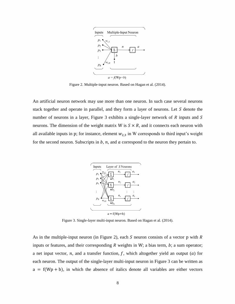
An artificial neuron may use more than one input (see Figure 2). In this case the input is not

a scalar but a vector, , of length , with each element corresponding to a feature or

attribute of an observation. Each input in vector is weighted by its corresponding element

in the weight matrix , and the neuron output can be written as .

8

Figure 2. Multiple-input neuron. Based on Hagan et al. (2014).

An artificial neuron network may use more than one neuron. In such case several neurons

stack together and operate in parallel, and they form a layer of neurons. Let denote the

number of neurons in a layer, Figure 3 exhibits a single-layer network of inputs and

neurons. The dimension of the weight matrix is , and it connects each neuron with

all available inputs in ; for instance, element in W corresponds to third input’s weight

for the second neuron. Subscripts in , , and correspond to the neuron they pertain to.

Figure 3. Single-layer multi-input neuron. Based on Hagan et al. (2014).

As in the multiple-input neuron (in Figure 2), each neuron consists of a vector with

inputs or features, and their corresponding weights in ; a bias term, ; a sum operator;

a net input vector, , and a transfer function, , which altogether yield an output ( ) for

each neuron. The output of the single-layer multi-input neuron in Figure 3 can be written as

, in which the absence of italics denote all variables are either vectors

9

( ) or matrices ( ). The number of neurons ( ) in a single-layer neuron is

determined by the number of outputs; for instance, a single-layer neuron with x outputs

requires x neurons.

Several layers may be used within the artificial neural network. Figure 4 displays a three-

layer network. In this case for each layer there is a weight matrix, ; a bias vector, ; a net

input vector, ; a transfer function vector, , and an output vector, , with superscripts and

subscripts denoting the number of the layer and the neuron, respectively. The number of

neurons may vary across layers, thus each layer has its own denoted with a superscript. It

is customary to refer to the final layer as the output layer (i.e. the layer that yields the

output of the network), whereas the other layers are referred to as hidden layers; hence, the

artificial neural network in Figure 4 has two hidden layers and one output layer.

Figure 4. Three-layer multi-input neuron. Based on Hagan et al. (2014).

There is a reason to increase the number of layers in artificial neural networks. Multi-layer

networks are more powerful than single-layer networks as they can be trained to

approximate most functions well (Hagan et al., 2014). That is, multi-layer artificial neural

networks, given enough hidden layers and enough training samples, can closely

approximate any function (Han & Kamber, 2006). As each hidden layer may accommodate

10

an arbitrary number of neurons, increasing the number of layers above the single-layer case

allows setting an arbitrary number of neurons too.7

Regarding the number of neurons in the output layer of a multi-layer neuron, this is

determined by the type of problem and the number of elements in the target vector. In the

case of continuous variables the number of neurons in the output equals the number of

targets. In the case of discrete variables (i.e. classification problems) with two classes (e.g.

YES or NO) a single-neuron output is required. If there are more than two classes, then one

output neuron per class is used (Han & Kamber, 2006).

3.2. Training the artificial neural network

As stated, the learning process of an artificial neural neuron consists of adjusting

parameters in W and b in order to attain an input-output relationship target under the

chosen transfer functions in f for a set of observations. This process is also called training,

and is somewhat similar to fitting the parameters of a regression model in econometrics; in

fact, from a statistical point of view, artificial neural networks perform non-linear

regression (Han & Kamber, 2006).

However, unlike typical applications of regression models in econometrics, artificial neural

networks are intended for prediction. As depicted by Varian (2014), econometrics is

concerned with detecting and summarizing relationships in data, with regression analysis as

its prevalent tool. Meanwhile, machine learning methods –such as artificial neural

networks- are concerned with developing high-performance computer systems that can

provide useful predictions, namely out-of-sample predictions. That is, following Shmueli

(2010), traditional econometrics is intended for exploratory modeling (i.e. testing causal

theory), whereas artificial neural networks aim at capturing complicated associations and

leading to accurate predictions (i.e. predictive modeling).

7 As reported by Hagan et al. (2004), the number of layers in most practical artificial neural networks is just

two or three. It is common to refer to the training of artificial neural networks with numerous hidden layers as

deep learning. Regarding the number of neurons in hidden layers, Hagan et al. highlight that there are few

problems in which there may be an optimal number of neurons, and determining such optimal is an active

area of research. Hastie et al. (2013) reports a 5 to 100 range for the number of neurons in hidden layers,

increasing with the number of inputs and the number of training cases.

11

Also, unlike classic econometric models, in the artificial neural network model there is no

specific hypothesis about the value of the parameters, and most of the time they may not be

interpreted (McNelis, 2005). Moreover, artificial neural networks make no assumptions

about the statistical distribution or properties of the data, and they are able to deal with non-

linear relationships between factors in the data (see Zhang et al. (1999), McNelis (2005),

Demyanyk & Hasan (2009), and Nazari & Alidadi (2013)).

The most popular artificial neural network learning algorithm is backpropagation

(Mitchell, 1997; Han & Kamber, 2006). Backpropagation learns by iteratively processing a

dataset of training examples (i.e. observations), comparing network’s prediction (i.e.

output) for each example with the actual target value. Parameters in W and b are modified

in backwards direction, from the output layer, through each hidden layer down to the first

hidden layer –hence its name (Han & Kamber, 2006). Backpropagation usually employs

some type of gradient descent method to minimize the error between the prediction and the

actual target value.8

Regarding error minimization, there are two main measures of performance. For predicting

continuous variables the fit of the artificial neural network is typically measured as the sum

(or the mean) of squared errors. For classification, where targets are discrete values, the

cross-entropy is preferred (see Bishop (1995) and Hagan et al. (2014)); yet, some authors

use the sum (or the mean) of squared errors for classification problems as well (e.g. Zhang

et al. (1999) and Brédart (2014)). Let denote the number of examples or observations

used to train the algorithm; the number of neurons in the output layer of the artificial

neural network; the actual target value for neuron in example , and the predicted

(i.e. output) value for neuron in example , the sum of squared errors ( ) and the cross-

entropy ( ) are defined as in [1] and [2], respectively. In the case of sum of squared errors

and are continuous values, whereas in cross-entropy they are limited to 0 and 1

values.9

8 As the characteristics of our classification problem match those stated by Mitchell (1997), backpropagation

is an appropriate learning algorithm. A complete explanation on the functioning of the backpropagation

algorithm or gradient descent is outside the scope of our paper. The interested reader may refer to Bishop

(1995), Mitchell (1997), and Han and Kamber (2006). 9 As in Bishop (1995), in [2] is a function that is non-negative, and which equals zero when .

12

∑∑( )

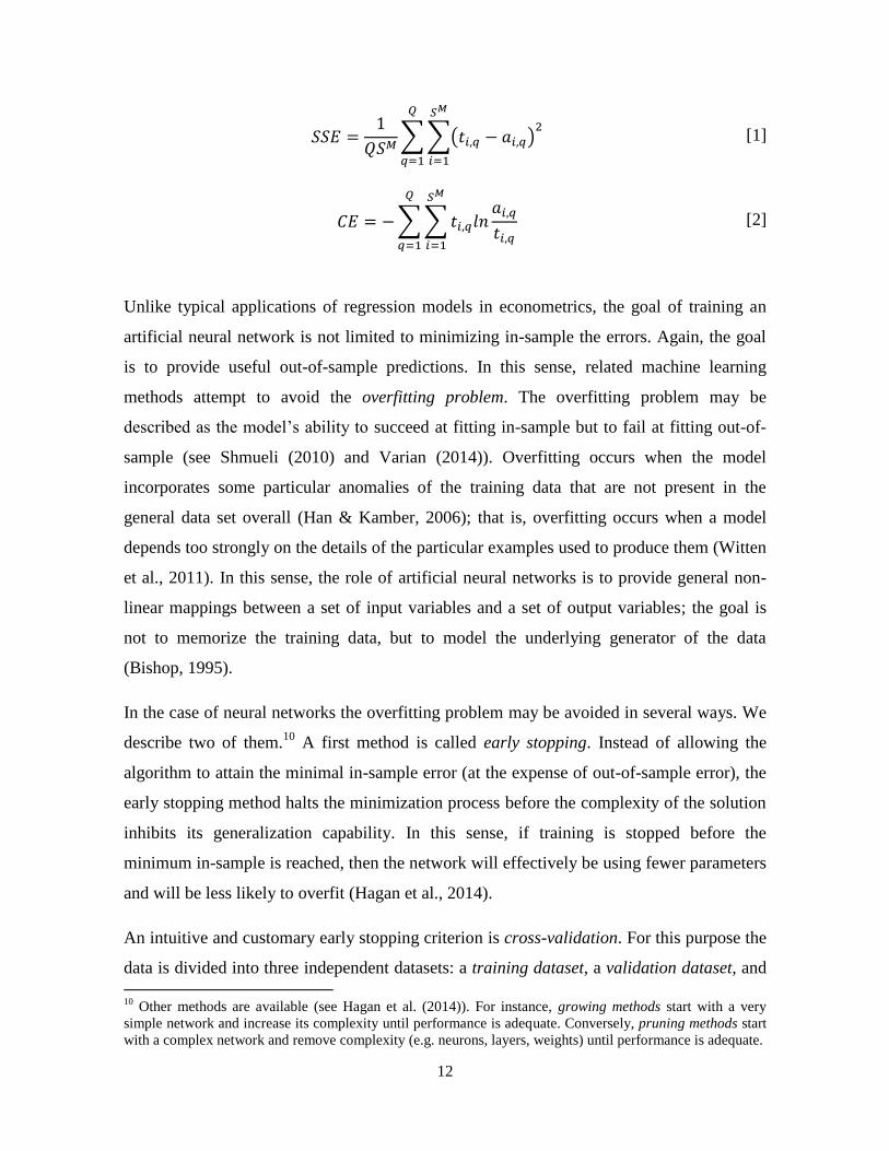
[1]

∑∑

[2]

Unlike typical applications of regression models in econometrics, the goal of training an

artificial neural network is not limited to minimizing in-sample the errors. Again, the goal

is to provide useful out-of-sample predictions. In this sense, related machine learning

methods attempt to avoid the overfitting problem. The overfitting problem may be

described as the model’s ability to succeed at fitting in-sample but to fail at fitting out-of-

sample (see Shmueli (2010) and Varian (2014)). Overfitting occurs when the model

incorporates some particular anomalies of the training data that are not present in the

general data set overall (Han & Kamber, 2006); that is, overfitting occurs when a model

depends too strongly on the details of the particular examples used to produce them (Witten

et al., 2011). In this sense, the role of artificial neural networks is to provide general non-

linear mappings between a set of input variables and a set of output variables; the goal is

not to memorize the training data, but to model the underlying generator of the data

(Bishop, 1995).

In the case of neural networks the overfitting problem may be avoided in several ways. We

describe two of them.10

A first method is called early stopping. Instead of allowing the

algorithm to attain the minimal in-sample error (at the expense of out-of-sample error), the

early stopping method halts the minimization process before the complexity of the solution

inhibits its generalization capability. In this sense, if training is stopped before the

minimum in-sample is reached, then the network will effectively be using fewer parameters

and will be less likely to overfit (Hagan et al., 2014).

An intuitive and customary early stopping criterion is cross-validation. For this purpose the

data is divided into three independent datasets: a training dataset, a validation dataset, and

10

Other methods are available (see Hagan et al. (2014)). For instance, growing methods start with a very

simple network and increase its complexity until performance is adequate. Conversely, pruning methods start

with a complex network and remove complexity (e.g. neurons, layers, weights) until performance is adequate.

13

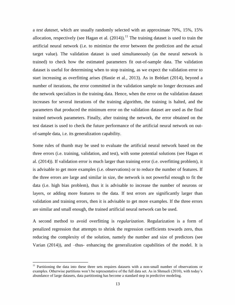
a test dataset, which are usually randomly selected with an approximate 70%, 15%, 15%

allocation, respectively (see Hagan et al. (2014)).11

The training dataset is used to train the

artificial neural network (i.e. to minimize the error between the prediction and the actual

target value). The validation dataset is used simultaneously (as the neural network is

trained) to check how the estimated parameters fit out-of-sample data. The validation

dataset is useful for determining when to stop training, as we expect the validation error to

start increasing as overfitting arises (Hastie et al., 2013). As in Brédart (2014), beyond a

number of iterations, the error committed in the validation sample no longer decreases and

the network specializes in the training data. Hence, when the error on the validation dataset

increases for several iterations of the training algorithm, the training is halted, and the

parameters that produced the minimum error on the validation dataset are used as the final

trained network parameters. Finally, after training the network, the error obtained on the

test dataset is used to check the future performance of the artificial neural network on out-

of-sample data, i.e. its generalization capability.

Some rules of thumb may be used to evaluate the artificial neural network based on the

three errors (i.e. training, validation, and test), with some potential solutions (see Hagan et

al. (2014)). If validation error is much larger than training error (i.e. overfitting problem), it

is advisable to get more examples (i.e. observations) or to reduce the number of features. If

the three errors are large and similar in size, the network is not powerful enough to fit the

data (i.e. high bias problem), thus it is advisable to increase the number of neurons or

layers, or adding more features to the data. If test errors are significantly larger than

validation and training errors, then it is advisable to get more examples. If the three errors

are similar and small enough, the trained artificial neural network can be used.

A second method to avoid overfitting is regularization. Regularization is a form of

penalized regression that attempts to shrink the regression coefficients towards zero, thus

reducing the complexity of the solution, namely the number and size of predictors (see

Varian (2014)), and –thus- enhancing the generalization capabilities of the model. It is

11

Partitioning the data into these three sets requires datasets with a non-small number of observations or

examples. Otherwise partitions won’t be representative of the full data set. As in Shmueli (2010), with today’s

abundance of large datasets, data partitioning has become a standard step in predictive modeling.

14

analogous to adding a penalty to the error function (e.g. [1] or [2]) based on the size of the

parameters, or weight decay (see Mitchell (1997) and Hastie et al. (2013)).

3.3. Post-training analysis

After training the artificial neural network with early stopping by cross-validation there are

three sets of outputs, corresponding to the training, validation and test datasets. For each set

of outputs there are several measures or tests to assess the quality and usefulness of the

trained artificial neural network.

For predicting continuous variables it is customary to use fit-type measures. For instance, it

is common to display how the predicted value fits the actual target value (e.g. a scatter plot,

a histogram of their differences), to compute a regression between them, or to compute

their correlation coefficient or regression’s r2. For classification problems, in which

variables are discrete values, other measures are used. The main objective of these other

measures is to reveal the extent to which the artificial neural network (mis)classifies the

data. As presented in Hagan et al. (2004), there are two main measures: the confusion

matrix and the receiver operating characteristic (ROC) curve.

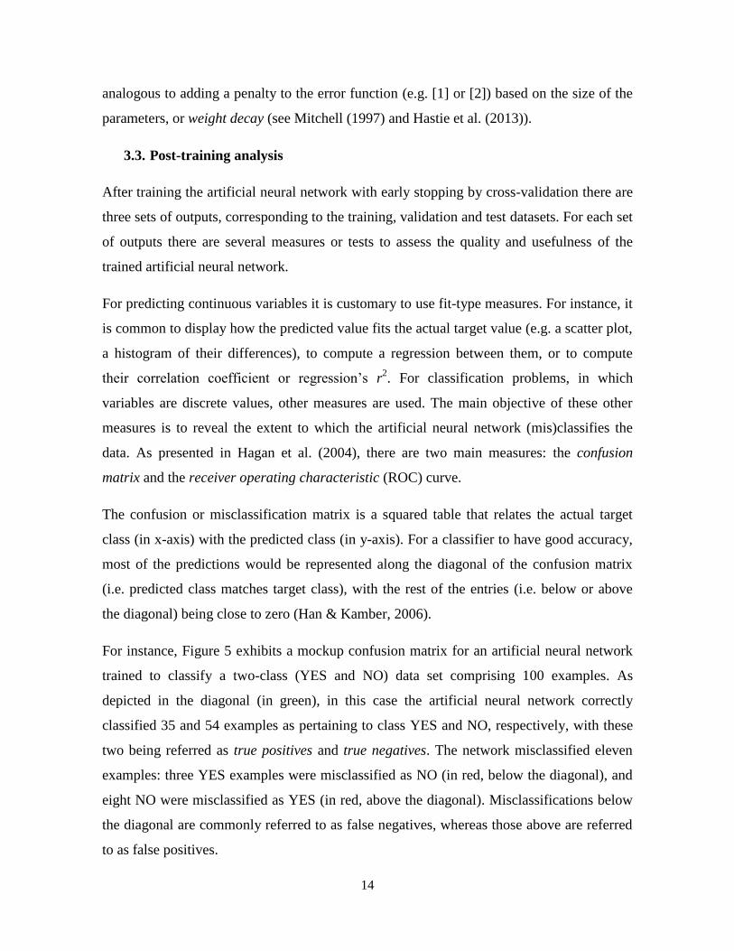
The confusion or misclassification matrix is a squared table that relates the actual target

class (in x-axis) with the predicted class (in y-axis). For a classifier to have good accuracy,

most of the predictions would be represented along the diagonal of the confusion matrix

(i.e. predicted class matches target class), with the rest of the entries (i.e. below or above

the diagonal) being close to zero (Han & Kamber, 2006).

For instance, Figure 5 exhibits a mockup confusion matrix for an artificial neural network

trained to classify a two-class (YES and NO) data set comprising 100 examples. As

depicted in the diagonal (in green), in this case the artificial neural network correctly

classified 35 and 54 examples as pertaining to class YES and NO, respectively, with these

two being referred as true positives and true negatives. The network misclassified eleven

examples: three YES examples were misclassified as NO (in red, below the diagonal), and

eight NO were misclassified as YES (in red, above the diagonal). Misclassifications below

the diagonal are commonly referred to as false negatives, whereas those above are referred

to as false positives.

15

Pre

dic

ted

cla

ss YES

35

35.0%

8

8.0% 81.4%

18.6%

NO 3

3.0%

54

44.0% 94.7%

5.3%

92.1%

7.9%

87.1%

12.9%

89.0%

11.0%

YES NO

Target class

Figure 5. Confusion matrix. Based on Hagan et al. (2014).

The column farther to the right exhibits the precision of the classifier, which corresponds to

the ratio of true positives to predicted positives. In this case, the precision for classifying

positives is 35/43=81.4%; its complement (1-81.4%=18.6%) is reported below. The row

farther to the bottom exhibits the recall of the classifier for each class, which corresponds

to the ratio of true positives to actual positives. In this case, the recall for classifying

positives is 35/38=92.1%. The lower right position in the confusion matrix displays the

ratio of successful classifications (i.e. true positives and true negatives) to the number of

observations, i.e. (35+54)/100=89.0%.

The receiver operating characteristic (ROC) is a curve that shows the trade-off between the

true positive rate (in y-axis) and the false-positive rate (in x-axis) for a given model (Han &

Kamber, 2006). If the model is accurate we are more likely to encounter true positives than

false positives, thus a steep ROC curve (i.e. close to the y-axis) is expected. The closer the

ROC curve to the diagonal of the plot, the less accurate the model (i.e. it is close to a

random guess).

4. Data and methodology

As depicted before, we use an artificial neural network pattern recognition method on

Colombian banks’ monthly balance sheet data to test whether it is possible to classify them

with fair accuracy. Each balance sheet in our dataset comprises 25 features or attributes of a

bank, corresponding to a two-digit filtering of its financial statements reported to the

16

Colombian Financial Superintendency. These 25 features are continuous variables that

pertain to assets (9), liabilities (9), and equity accounts (7), as exhibited in Table 3 (in

Appendix). Balance sheets are available on a monthly basis. These 25 features conform to

the basic breakdown that the Basel Committee on Banking Supervision points out as an

essential breakdown of a bank’s financial position for supervisory purposes (see BCBS

(1998)).12

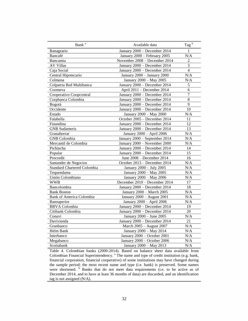
The dataset comprises 21 banks and their corresponding 25 features, from January 2000 to

December 2014, with 3,237 examples in total. Because from January 2015 banks have

changed reporting standards to International Financial Reporting Standards (IFRS), balance

sheet data after 2014 is discarded for consistency issues. Despite balance sheet data for

about 41 banks exists from January 2000 to December 2014, we work with those that are

active as of December 2014 and that have at least three years of data (i.e. 36 balance sheets)

only; this choice attempts to preserve the relevance of results to active banks, and to work

with non-small datasets. With this choice most banks have 180 balance sheets, whereas the

bank with the least has 45. The list of selected and discarded banks is presented in Table 4

(in Appendix).

The dataset may be represented as a matrix of 25 features (in rows) and 3,237 examples

(in columns), as in [3]. This dataset is the input to our artificial neural network, with

element corresponding to the second feature of the first example. Matrix of actual

target values [4] contains the class (e.g. the label of the bank) corresponding to each

example (in columns) as a 21-element binary code. For instance, in [4] labels the

first example (in the first column) as Bank 1, whereas labels the last example

(in the last column) as Bank 21; as each example in our dataset may belong to one, and

only one, bank, each column in may only have a single element equal to 1.

12

It is possible to work with less features by choosing a set of relevant financial ratios (e.g. leverage, current

ratio, working capital), either supported by their popularity in related literature or by using a selection

criterion. By using the 25 features we avoid selection problems, and allow the entire data to work for the

model. Moreover, the 25 features, 3,237 examples, and the chosen artificial neural network, do not entail a

major computational challenge for the Matlab® Neural Network Toolbox running in a desktop computer.

17

[

]

[3]

[

]

[4]

Regarding our choice of artificial neural network (see Figure 6), we implement a standard

two-layer network, with one hidden layer and one output layer. Often a single hidden layer

is all that is necessary (see Zhang et al., (1999), Witten et al. (2011)), and it is the most

commonly used artificial neural network in economic and financial applications (McNelis,

2005). As usual, our learning algorithm is backpropagation.

Figure 6. Two-layer multi-input neuron. Based on Hagan et al. (2014).

In our case the artificial neural network comprises the inputs (i.e. a 25-account balance

sheet data for each bank, ), and a 21-neuron output layer (second layer, ).

18

In our base case scenario we arbitrarily set the number of neurons in the hidden layer to

fifteen (first layer, ); other scenarios, with different numbers of neurons (i.e. 5, 10,

20, 25), are also reported for comparison. Akin to each column in the actual target value

matrix ( ), the output vector ( ) for each bank is a 21-element binary code, in which there

is only one element different from zero, corresponding to the target classification of the

balance sheet. The transfer function in the hidden layer ( ) is a customary log-sigmoid

function, whereas the transfer function in the output layer ( ) is a softmax function13

. As

this is a classification problem, the cross-entropy [2] fitness measure is preferred.

During training the artificial neural network will learn how the different features in the 25-

account balance sheet data serve the purpose of classifying the banks. That is, the artificial

neural network will learn the parameters that allow classifying banks best based on their

accounting data. After training, given a set of out-of-sample balance sheet (i.e. observations

not used for training nor validation), the artificial neural network will be able to identify to

which one of the 21 banks those balance sheets belongs. In this sense, the artificial neural

network will perform pattern recognition (i.e. classification) of banks based on balance

sheet data.

About our choice for avoiding overfitting, we use early stopping by cross-validation; as

exhibited in the results, additional methods (e.g. regularization) to avoid overfitting are not

required. Therefore, following Hagan et al. (2014), we randomly partition the data into

three sets (training, validation, test), with an approximate 70%, 15%, 15% allocation. With

this partition, training, validation, and test datasets will comprise 2,265, 486, and 486

examples, respectively.

5. Main results

The overall results of the training process are exhibited in Table 1. The artificial neural

network misclassifies 0.35% of the training examples, about 8 balance sheets out of 2,265.

13

A softmax function is interesting for our classification purposes as its outcome can be interpreted as the

probabilities associated with each class, and it is convenient as we use cross-entropy as our error measure (see

Bishop (1995) and Hagan et al. (2014)). The softmax function is computed as ∑ ⁄ .

19

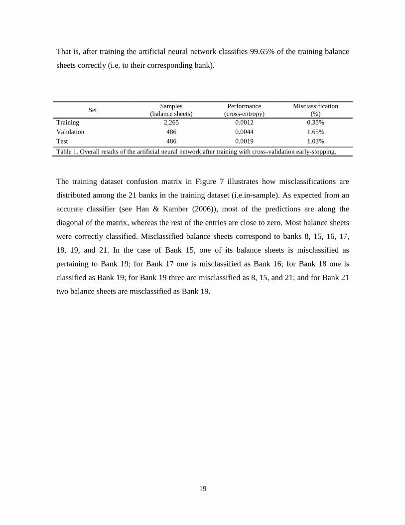
That is, after training the artificial neural network classifies 99.65% of the training balance

sheets correctly (i.e. to their corresponding bank).

Set Samples

(balance sheets)

Performance

(cross-entropy)

Misclassification

(%)

Training 2,265 0.0012 0.35%

Validation 486 0.0044 1.65%

Test 486 0.0019 1.03%

Table 1. Overall results of the artificial neural network after training with cross-validation early-stopping.

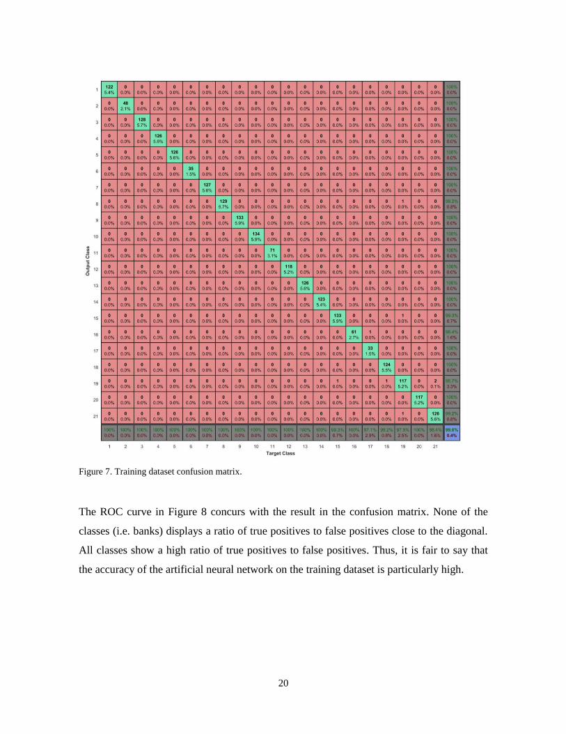
The training dataset confusion matrix in Figure 7 illustrates how misclassifications are

distributed among the 21 banks in the training dataset (i.e.in-sample). As expected from an

accurate classifier (see Han & Kamber (2006)), most of the predictions are along the

diagonal of the matrix, whereas the rest of the entries are close to zero. Most balance sheets

were correctly classified. Misclassified balance sheets correspond to banks 8, 15, 16, 17,

18, 19, and 21. In the case of Bank 15, one of its balance sheets is misclassified as

pertaining to Bank 19; for Bank 17 one is misclassified as Bank 16; for Bank 18 one is

classified as Bank 19; for Bank 19 three are misclassified as 8, 15, and 21; and for Bank 21

two balance sheets are misclassified as Bank 19.

20

Figure 7. Training dataset confusion matrix.

The ROC curve in Figure 8 concurs with the result in the confusion matrix. None of the

classes (i.e. banks) displays a ratio of true positives to false positives close to the diagonal.

All classes show a high ratio of true positives to false positives. Thus, it is fair to say that

the accuracy of the artificial neural network on the training dataset is particularly high.

21

Figure 8. Training dataset ROC.

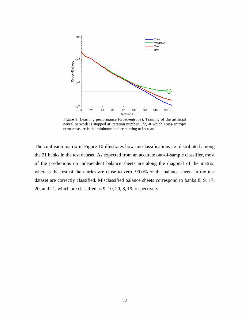
As exhibited in Figure 9, training is stopped at iteration number 172 to avoid overfitting; at

this iteration the validation error is the minimum before starting to increase for several

iterations. As exhibited in Table 1, validation error for the artificial neural network equals a

misclassification of 1.65% balance sheets, about 8 balance sheets out of 486 in the

validation dataset. When the artificial neural network is used to classify the test dataset (i.e.

a set of 486 balance sheets not used during training or validation), it misclassifies 1.03% of

the sample, about 5 out of 486.

22

Figure 9. Learning performance (cross-entropy). Training of the artificial

neural network is stopped at iteration number 172, at which cross-entropy

error measure is the minimum before starting to increase.

The confusion matrix in Figure 10 illustrates how misclassifications are distributed among

the 21 banks in the test dataset. As expected from an accurate out-of-sample classifier, most

of the predictions on independent balance sheets are along the diagonal of the matrix,

whereas the rest of the entries are close to zero. 99.0% of the balance sheets in the test

dataset are correctly classified. Misclassified balance sheets correspond to banks 8, 9, 17,

20, and 21, which are classified as 9, 10, 20, 8, 19, respectively.

23

Figure 10. Test dataset confusion matrix

Again, the ROC curve in Figure 11 concurs with the result in the test dataset confusion

matrix. None of the classes (i.e. banks) displays a ratio of true positives to false positives

close to the diagonal. All classes show a high ratio of true positives to false positives. Thus,

it is fair to say that the accuracy of the artificial neural network on the test dataset is high as

well. That is, the out-of-sample classification capability of the artificial neural network is

good.

24

Figure 11. Test dataset ROC

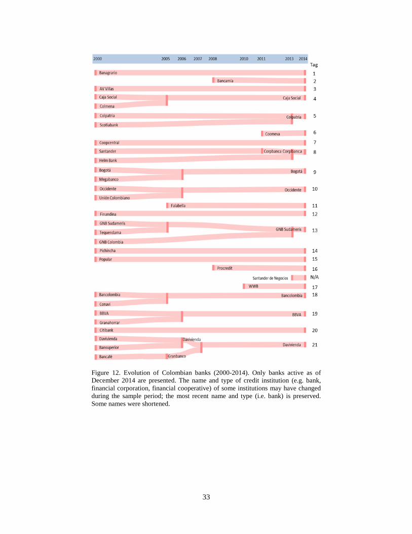
Regarding those banks that are misclassified in the training or test dataset (i.e. banks 8, 9,

10, 17, 19, 20, and 21), there are two relevant traits. First, most of them (i.e. banks 8, 9, 10,

19, 21) merged with or acquired some other bank(s) during the period under analysis, as

depicted in Figure 12 (in Appendix). Second, bank 17 has been incorporated as a bank

rather recently (see Table 4 and Figure 12, in Appendix), thus the number of balance sheets

is lower than for most banks. Only bank 20 does not conform to these two traits.

About the first trait, it is likely that abrupt changes in the main features of the examples, as

those that may be caused by merging with or acquiring other bank(s), may affect the ability

of the artificial neural network to generalize. About the second, smaller datasets may

impose difficulties in the training process as well. Nevertheless, as misclassifications are

exceptional, about 0.35% and 1.03% in the training and test datasets, respectively, the

resulting artificial neural network may be considered safe to use for our main purpose: to

perform pattern recognition (i.e. classification) of banks based on balance sheet data.

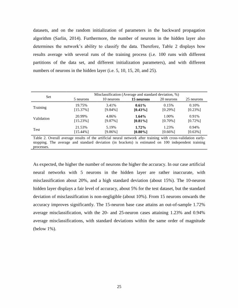
Results in artificial neural networks are dependent on several items. For instance, they are

dependent on the random partition of the dataset into the training, validation and test

25

datasets, and on the random initialization of parameters in the backward propagation

algorithm (Sarlin, 2014). Furthermore, the number of neurons in the hidden layer also

determines the network’s ability to classify the data. Therefore, Table 2 displays how

results average with several runs of the training process (i.e. 100 runs with different

partitions of the data set, and different initialization parameters), and with different

numbers of neurons in the hidden layer (i.e. 5, 10, 15, 20, and 25).

Set Misclassification (Average and standard deviation, %)

5 neurons 10 neurons 15 neurons 20 neurons 25 neurons

Training 19.75%

[15.37%]

3.41%

[9.84%] 0.61%

[0.43%]

0.15%

[0.29%]

0.10%

[0.23%]

Validation 20.99%

[15.23%]

4.86%

[9.87%] 1.64%

[0.81%]

1.00%

[0.70%]

0.91%

[0.72%]

Test 21.53%

[15.44%]

5.19%

[9.86%] 1.72%

[0.80%]

1.23%

[0.66%]

0.94%

[0.63%]

Table 2. Overall average results of the artificial neural network after training with cross-validation early-

stopping. The average and standard deviation (in brackets) is estimated on 100 independent training

processes.

As expected, the higher the number of neurons the higher the accuracy. In our case artificial

neural networks with 5 neurons in the hidden layer are rather inaccurate, with

misclassification about 20%, and a high standard deviation (about 15%). The 10-neuron

hidden layer displays a fair level of accuracy, about 5% for the test dataset, but the standard

deviation of misclassification is non-negligible (about 10%). From 15 neurons onwards the

accuracy improves significantly. The 15-neuron base case attains an out-of-sample 1.72%

average misclassification, with the 20- and 25-neuron cases attaining 1.23% and 0.94%

average misclassifications, with standard deviations within the same order of magnitude

(below 1%).

26

6. Final remarks

Based on the well-documented effectiveness of artificial neural networks as classifiers, and

spurred by their recent disruption as a wide-ranging powerful machine learning tool, we

successfully implemented a pattern recognition method based on Colombian banks’ balance

sheet data. For our base case (i.e. a 15-neuron hidden layer artificial neural network) in-

sample and out-of-sample accuracy is high; misclassifications are below 2% in training and

test datasets.

Our work contributes to related literature. Results demonstrate that balance sheets are

unique and representative snapshots of banks, akin to individuals’ photographs in a facial

recognition problem. Also, results demonstrate that banks’ pattern recognition based on

their balance sheets by means of training a basic artificial neural network is possible.

Furthermore, to the best of our knowledge, we are the first to successfully employ raw

balance sheet data –instead of selected financial ratios- for firm’s classification problems.

Avoiding selection bias by working with raw balance sheets may be particularly useful and

convenient for risk management and supervisory purposes.

Some potential byproducts of our findings are worth discussing. As accurate banks’ pattern

recognition on balance sheet data is possible, it is reasonable to implement artificial neural

network models to develop early-warning systems that detect unusual changes in banks’

financial statements. This may be useful for flagging anomalies or changes in trends –say,

caused by deteriorating financial conditions or by some types of misreporting (e.g. fraud,

errors). Moreover, if coupled with fair indicators of financial distress (e.g. unusually high

money market interest rates, risk rating downgrades, bankruptcy), an artificial neural

network model on raw balance sheet data may be useful for classifying banks (or firms)

according to their fragility, while mitigating selection bias arising from the selection of

adequate financial ratios. Likewise, it is also reasonable to examine whether a banking

system’s snapshot (e.g. a stacked version of all bank’s balance sheets) may be useful for

flagging system-wide anomalies or changes in trends.

Beyond the classification of financial or non-financial firms, the application of artificial

neural networks to early-warning systems is broad and challenging enough to foresee that

27

using raw data for classifying countries may be convenient as well. For instance, the works

of Fioramanti (2008), Sarlin (2014), and Holopainen and Sarlin (2016) may profit from

using raw data (e.g. balance of payments, fiscal balances, and interbank networks) for

predicting the arrival of banking, currency or debt crises.

Our results also pose some challenges. For instance, based on the good results with balance

sheet data, it is likely that other potential sources of abundant, unique, and characteristic

data, such as payments, exposures, or trades, may be particularly helpful for classification

or prediction purposes. Mixtures of data sources (e.g. balance sheets, financial ratios,

payments, exposures, trades) may also provide richer datasets to work with. However, due

to the vast amount of examples and features contained in such datasets, a qualitative leap in

the model may be required, possibly involving deep learning artificial neural networks (e.g.

many hidden layers, with many neurons).

Finally, some limitations of our work should be stated, which carry some potential research

extensions. First, as new accounting standards were adopted since 2015, updating our work

will require a potentially grim process of making both standards comparable. Second, due

to some accounting standards differences among distinct types of financial institutions

before 2015, our work comprises banks only; despite banks are the focus of financial

literature, it is advisable to include non-bank credit institutions and non-credit institutions.

Third, off-balance sheet positions of banks are not included in our dataset. Fourth, a

common assumption on pattern recognition is that data does not evolve with time (see

Bishop (1995)), which is a problematic assumption in our case. Therefore, it is important to

incorporate the non-stationary nature of balance sheets when designing and developing

specific applications of artificial neural networks for pattern recognition; for instance, in an

early-warning system the test dataset may not be randomly selected from the entire dataset,

but should correspond to those arriving as new information.

28

7. References

Angelini, E., di Tollo, G., & Roli, A. (2008) A Neural Network Approach for Credit Risk

Evaluation. The Quarterly Review of Economics and Finance, 48, 733-755.

doi:10.1016/j.qref.2007.04.001

Atiya, A.F. (2001) Bankruptcy Prediction for Credit Risk Using Neural Networks: A

Survey and New Results. IEEE Transactions on Neural Networks, 12 (4), 929-935.

Basel Committee on Banking Supervision (1997) Core Principles for Effective Banking

Supervision, September.

Basel Committee on Banking Supervision (1998) Enhancing Banking Transparency,

September.

Bekhet, A.H. & Eletter, S.F. (2014) Credit Risk Assessment Model for Jordanian

Commercial Banks: Neural Scoring Approach. Review of Development Finance, 4,

20-28. doi:10.1016/j.rdf.2014.03.002

Bishop, C.M. (1995). Neural Networks for Pattern Recognition. Clarendon Press: Oxford.

Brédart, X. (2014) Bankruptcy Prediction Model Using Neural Networks. Accounting and

Finance Research, 3 (2), 124-128. doi:10.5430/afr.v3n2p124

Chisholm, A. (2002) An Introduction to Capital Markets. John Wiley & Sons: Chichester.

Demyanyk, Y. & Hasan, I. (2009) Financial Crises and Bank Failures: A Review of

Prediction Methods. Federal Reserve Bank of Cleveland Working Papers Series, 09-

04R, September.

Eletter, S.F., Yaseen, S.G, & Elrefae, G.A. (2010) Neuro-based Artificial Intelligence

Model for Loan Decisions. American Journal of Economics and Business

Administration, 2 (1), 27-34.

Fioramanti, M. (2008) Predicting sovereign Debt Crises Using Artificial Neural Networks:

A Comparative Approach. Journal of Financial Stability, 4, 149-164.

doi:10.1016/j.jfs.2008.01.001

Hagan, M.T., Demuth, H.B., Beale, M.H, & De Jesús, O. (2014) Neural Network Design.

Martin Hagan: Oklahoma.

29

Han, J. & Kamber, M. (2006) Data Mining: Concepts and Techniques. Morgan Kaufman

Publishers: San Francisco.

Hastie, T., Tibshirani, R., & Friedman, J. (2013) The Elements of Statistical Learning.

Springer: New York.

Holopainen, M. & Sarlin, P. (2016) Toward Robust Early-Warning Models: A Horse Race,

Ensembles and Model Uncertainty. ECB Working Paper, 1900, European Central

Bank, April.

Kaliski, B.S. (2001) Encyclopedia of Business and Finance. Macmillan Reference USA:

New York.

Khediri, K.B., Charfeddine, L., & Youssef, S.B. (2015) Islamic Versus Conventional Banks

in the GCC Countries: A Comparative Study Using Classification Techniques.

Research in International Business and Finance, 33, 75-98.

doi:10.1016/j.ribaf.2014.07.002

McNelis, P.D. (2005) Neural Networks in Finance. Elsevier: Burlington.

Mishkin, F.S. (2004) The Economics of Money, Banking, and Financial Markets. Pearson:

Boston.

Mitchell, T.M. (1997) Machine Learning. McGraw-Hill: Boston.

Nazari, M. & Alidadi, M. (2013) Measuring Credit Risk of Bank Customers Using

Artificial Neural Network. Journal of Management Research, 5 (2), 17-27.

Olmeda, I. & Fernández, E. (1997) Hybrid Classifiers for Financial Multicriteria Decision

Making: The Case of Bankruptcy Prediction. Computational Economics, 10, 317-

355.

Rudorfer, G. (1995) Early Bankruptcy Detection Using Neural Networks. APL Proceedings

of the International Conference on Applied Programming Languages, 171-178.

doi:10.1145/206913.206999

Salchenberger, L, Mine, C., & Lash, N. (1992) Neural Networks: A Tool for Predicting

Thrift Failures. Decision Science, 23, 899-916.

Sarlin, P. (2014) On Biologically Inspired Predictions of the Global Financial Crisis.

Neural Computing and Applications, 24 (3), 663-673. doi:10.1007/s00521-012-1281-

y

30

Schmidhuber, J. (2015) Deep Learning in Neural Networks. Neural Networks, 61, 85-117.

doi:10.1016/j.neunet.2014.09.003

Shmueli, G. (2010) To Explain or to Predict?. Statistical Science, 25(3), 289-310.

doi:10.1214/10-STS330

Tam, K.Y. (1991) Neural Network Models and the Prediction of Bank Bankruptcy. Omega

19, 429-445.

Tam, K.Y. & Kiang, M. (1990) Predicting Bank Failures: A Neural Network Approach.

Applied Artificial Intelligence, 4, 265-282.

Turkan, S., Polat, E., & Gunay, S. (2011) Classification of Domestic and Foreign

Commercial Banks in Turkey Based on Financial Performances Using Linear

Discriminant Analysis, Logistic Regression and Artificial Neural Network Models.

Proceedings of the International Conference on Applied Economics - ICOAE 2011,

717-723.

Varian, H.R. (2014) Big Data: New Tricks for Econometrics. Journal of Economic

Perspectives, 28 (2), 3-28. doi: 10.1257/jep.28.2.3

Wilson, R.L. & Sharda, R. (1994) Bankruptcy Prediction Using Neural Networks. Decision

Support Systems, 11 (5), 545-557. doi:10.1016/0167-9236(94)90024-8

Witten, I.H., Frank, E., & Hall, M.A. (2011) Data Mining: Practical Machine Learning

Tools and Techniques. Morgan Kaufman Publishers: Burlington.

Wu, R.C. (1997) Neural Network Models: Foundations and Applications to an Audit

Decision Problem. Annals of Operations Research, 75, 291-301.

Zhang, G., Hu, M.Y, Patuwo, B.E., & Indro, D.C. (1999) Artificial Neural Networks in

Bankruptcy Prediction: General Framework and Cross-validation Analysis. European

Journal of Operational Research, 116, 16-32.

31

8. Appendix

Account name Account number

Ass

ets

Cash 110000

Money market assets 120000

Investment securities, net 130000

Loans and financial leases, net 140000

Customer’s acceptances and derivatives 150000

Accounts receivable 160000

Salable, foreclosed, returned assets and others 170000

Property and equipment 180000

Other assets 190000

Lia

bil

itie

s

Deposits and demand accounts 210000

Money market liabilities 220000

Customer’s acceptances and derivatives 230000

Borrowing from financial institutions and other financial obligations 240000

Accounts payable 250000

Issued debt securities 260000

Other liabilities 270000

Estimated liabilities and provisions 280000

Mandatory convertible bonds 290000

Eq

uit

y

Common shares 310000

Retained earnings 320000

Other reserves 330000

Equity surplus 340000

Net income from previous periods 350000

Net income 360000

Dividend paid in stocks 370000

Table 3. Banks’ balance sheet structure (2000-2014). Based on balance sheet data available from

Colombian Financial Superintendency under COLGAAP accounting standards.

32

Bank a Available data Tag

b

Banagrario January 2000 – December 2014 1

Bancafé January 2000 – February 2005 N/A

Bancamia November 2008 – December 2014 2

AV Villas January 2000 – December 2014 3

Caja Social January 2000 – December 2014 4

Central Hipotecario January 2000 – January 2000 N/A

Colmena January 2000 – May 2005 N/A

Colpatria Red Multibanca January 2000 – December 2014 5

Coomeva April 2011 – December 2014 6

Cooperativo Coopcentral January 2000 – December 2014 7

Corpbanca Colombia January 2000 – December 2014 8

Bogotá January 2000 – December 2014 9

Occidente January 2000 – December 2014 10

Estado January 2000 – May 2000 N/A

Falabella October 2005 – December 2014 11

Finandina January 2000 – December 2014 12

GNB Sudameris January 2000 – December 2014 13

Granahorrar January 2000 – April 2006 N/A

GNB Colombia January 2000 – September 2014 N/A

Mercantil de Colombia January 2000 – November 2000 N/A

Pichincha January 2000 – December 2014 14

Popular January 2000 – December 2014 15

Procredit June 2008 – December 2014 16

Santander de Negocios October 2013 – December 2014 N/A

Standard Chartered Colombia January 2000 – July 2005 N/A

Tequendama January 2000 – May 2005 N/A

Unión Colombiano January 2000 – May 2006 N/A

WWB December 2010 – December 2014 17

Bancolombia January 2000 – December 2014 18

Bank Boston January 2000 – March 2005 N/A

Bank of America Colombia January 2000 – August 2001 N/A

Bansuperior January 2000 – April 2006 N/A

BBVA Colombia January 2000 – December 2014 19

Citibank Colombia January 2000 – December 2014 20

Conavi January 2000 – June 2005 N/A

Davivienda January 2000 – December 2014 21

Granbanco March 2005 – August 2007 N/A

Helm Bank January 2000 – May 2014 N/A

Interbanco January 2000 – October 2001 N/A

Megabanco January 2000 – October 2006 N/A

Scotiabank January 2000 – May 2013 N/A

Table 4. Colombian banks (2000-2014). Based on balance sheet data available from

Colombian Financial Superintendency. a The name and type of credit institution (e.g. bank,

financial corporation, financial cooperative) of some institutions may have changed during

the sample period; the most recent name and type (i.e. bank) is preserved. Some names

were shortened. b Banks that do not meet data requirements (i.e. to be active as of

December 2014, and to have at least 36 months of data) are discarded, and an identification

tag is not assigned (N/A).

33

Figure 12. Evolution of Colombian banks (2000-2014). Only banks active as of

December 2014 are presented. The name and type of credit institution (e.g. bank,

financial corporation, financial cooperative) of some institutions may have changed

during the sample period; the most recent name and type (i.e. bank) is preserved.

Some names were shortened.

ogotá -