boreal spring southern hemisphere annular mode, indian

Boreal spring Southern Hemisphere Annular Mode, Indian Ocean sea

surface temperature, and East Asian summer monsoon

Sulan Nan,1,2 Jianping Li,3 Xiaojun Yuan,4 and Ping Zhao1,2

Received 29 February 2008; revised 23 October 2008; accepted 3 November 2008; published 22 January 2009.

[1] The relationships among the boreal spring Southern Hemisphere Annular Mode(SAM), the Indian Ocean (IO) sea surface temperature (SST), and East Asian summermonsoon (EASM) are examined statistically in this paper. The variability of boreal springSAM is closely related to the IO SST. When the SAM is in its strong positive phase inboreal spring, with low-pressure anomalies over the south pole and high-pressureanomalies over middle latitudes, SST over the subtropics and middle latitudes of the SouthIndian Ocean (SIO) increases, which persists into the summer. Following the positive SSTanomalies over the subtropics and midlatitudes of the SIO, SST in the equatorial IndianOcean and Bay of Bengal increases in summer. Moreover, the variability of SST in theequatorial Indian Ocean and Bay of Bengal is closely related to EASM. When SST in theequatorial Indian Ocean and Bay of Bengal increases, EASM tends to be weak. Thereforethe IO SST may play an important role bridging boreal spring SAM and EASM. Theatmospheric circulations and surface heat exchanges contribute to the SST anomalies inthe SIO. When the spring SAM is in its strong positive phases, the regional Ferrel Cellweakens, and the anomalous upward motions at 20�S–30�S cause an increase of lowcloud cover and downward longwave radiation flux. The surface atmospheric circulationsalso transport more (less) warmer (cooler) air from middle latitudes north of 50�S(high latitudes south of 60�S) into 50�S–60�S and warm the air, which reduces thetemperature difference between the ocean and atmosphere and consequently reducessensible heat flux from the ocean to atmosphere. The increased downward longwaveradiation and decreased sensible heat are responsible for the SST increase in the SIO. Theatmospheric circulation and surface heat flux anomalies are of opposite signs followingthe strong negative phases of SAM.

Citation: Nan, S., J. Li, X. Yuan, and P. Zhao (2009), Boreal spring Southern Hemisphere Annular Mode, Indian Ocean sea surface

temperature, and East Asian summer monsoon, J. Geophys. Res., 114, D02103, doi:10.1029/2008JD010045.

1. Introduction

[2] The Southern Hemisphere Annular Mode (SAM),referred to as Antarctic oscillation (AAO), is a patternwhich involves a zonally symmetric seesaw in sea levelpressure (SLP) and geopotential height between the south-ern polar region and middle latitudes. It explains the greatestproportion of the total variance of the Southern Hemisphere(SH) monthly SLP, zonal wind and geopotential height[Kidson, 1975; Rogers and van Loon, 1982; Gong andWang, 1999; Thompson and Wallace, 2000].[3] Many studies have analyzed the relationship between

the SAM and climate variability in the SH. Van den Broeke

and Van Lipzig [2002] indicated that the anomaly of SAMmay change the winter tropospheric vertical and meridionalcirculation and consequently surface air temperature in theEast Antarctica.Genthon et al. [2003] found the SAMsignal inAntarctic precipitation anomalies. The SAM also may influ-ence precipitation over southeastern SouthAmerica because ofthe atmospheric circulation [Silvestri and Vera, 2003].[4] The SAM variability not only has relation to the

climate systems at midlatitude–high latitudes of the SH[e.g., Reason and Rouault, 2005; England et al., 2006;Ummenhofer et al., 2008], but also the climate in theNorthern Hemisphere (NH). Studies [Nan and Li, 2003;Gao et al., 2003] found that strong positive SAM events inspring are followed by weak East Asian summer monsoon(EASM); and vice versa. The interaction between seasurface temperature (SST) in the Indian Ocean (IO) andAsian summer monsoon has been examined extensively.Numerical models indicated that the variability of Asiansummer monsoon is sensitive to the conditions of SST in thetropical southern IO [Zhu and Houghton, 1996]. Terray etal. [2003] pointed out that strong (weak) Indian summermonsoons are preceded by significant positive (negative)

JOURNAL OF GEOPHYSICAL RESEARCH, VOL. 114, D02103, doi:10.1029/2008JD010045, 2009ClickHere

for

FullArticle

1Chinese Academy of Meteorological Sciences, Beijing, China.2Laboratory for Climate Studies, China Meteorological Administration,

Beijing, China.3National Key Laboratory of Numerical Modeling for Atmospheric

Sciences and Geophysical Fluid Dynamics, Institute of AtmosphericPhysics, Chinese Academy of Sciences, Beijing, China.

4Lamont-Doherty Earth Observatory, Columbia University, Palisades,New York, USA.

Copyright 2009 by the American Geophysical Union.0148-0227/09/2008JD010045$09.00

D02103 1 of 13

http://dx.doi.org/10.1029/2008JD010045

SST anomalies in the southeastern subtropical IO duringboreal winter. Terray et al. [2005] further emphasized theimportance of the southern IO for an ENSO-monsoonrelationship. Kucharski et al. [2006] recently documentedthat in decadal timescale, cold (warm) Indian equatorialSST causes low-level divergence (convergence) that in turnmodifies the local Hadley circulation and strengthens(weakens) the Indian monsoon circulation. These studiesall indicate that the IO SST plays an important role in thevariability of the Asian monsoon.[5] The physical processes that link the IO SST variabil-

ity to atmospheric forcing have also been investigated. Kleinet al. [1999] pointed out that the warming of the IO surfacemay have been partly a response to remote forcing from thePacific. During El Nino events, an anomalously warm SSTin the central-eastern Pacific reduces cloud cover over theIO and allows in more solar radiation to warm the seasurface. Reason et al. [2000] demonstrated that the changesof wind in the IO affect SST through surface turbulent heatfluxes. Fauchereau et al. [2003] showed the dipole-like

SST variability in the South Indian and South Atlanticoceans in January–March. Hermes and Reason [2005]further pointed out that latent heat fluxes, upwelling, andEkman heat transports associated with SAM and a wavenumber 3 or 4 pattern contribute to the dipole-like SSTvariability. The interaction of southern midlatitude zonalwinds and ocean was also verified in GCM simulations[Watterson, 2000].[6] Current studies on the subject mainly focus on the

tropical IO. This paper emphasizes the importance of SSTover the subtropics and middle latitudes of the SouthernIO. The relationship of the spring SAM and EASM is investi-gated by analyzing the role of the IO SST in this teleconnection.[7] Data sets and methods of analysis used in this study

are described in section 2. The relationships among theboreal spring SAM, the IO SST and EASM are documentedin section 3. The connections among the SSTs in differentregions of the IO are examined in section 4. In section 5, weinvestigate possible physical processes that are responsiblefor connecting SST anomalies over the subtropics and

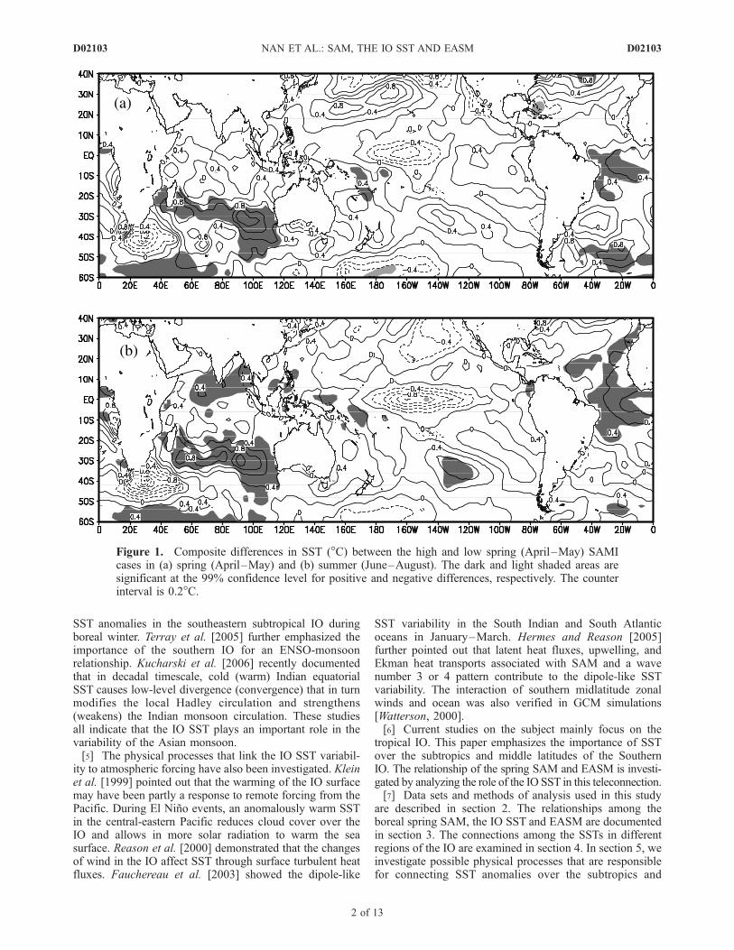
Figure 1. Composite differences in SST (�C) between the high and low spring (April–May) SAMIcases in (a) spring (April–May) and (b) summer (June–August). The dark and light shaded areas aresignificant at the 99% confidence level for positive and negative differences, respectively. The counterinterval is 0.2�C.

D02103 NAN ET AL.: SAM, THE IO SST AND EASM

2 of 13

D02103

Figure 2. Heterogeneous correlation patterns of the leading ESVD mode for the spring (April–May)SH SLP anomalies south of 10�S (top left) and the Indian Ocean SST anomalies from April to August,respectively. The areas with positive (negative) correlation coefficients that are significant at the 99%confidence level are shaded dark (light). The latitude lines in the top left are at a 20-degree intervalstarting from 10�S.


3 of 13

D02103

middle latitudes of the SIO and the spring SAM variability.On the basis of the above analyses, we summarize the roleof the IO SST in the relationship between the boreal springSAM and following EASM in section 6.

2. Data and Methods of Analysis

[8] We use several data sets in this study. Monthly meanSST data were obtained from National Climatic Data Center(NCDC) Extended Reconstructed Sea Surface Temperatures(ERSST) [Smith and Reynolds, 2004], with resolution of 2�latitude by 2� longitude covering 1958–2000. The SAMindex (SAMI) (1958–2000) is the difference in the normal-ized zonal mean SLP (from NCEP-NCAR) between 40�Sand 70�S [Nan and Li, 2003], which is a modification of theAntarctic Oscillation index defined by Gong and Wang[1999]. The East Asian summer monsoon (EASM) indexis a unified monsoon index (dynamical normalized season-ality), which is given by

d ¼ kV 1 � VikkV k

� 2

where V 1, Vi are the January climatological and monthlywind vectors at a point, respectively, V is the mean ofJanuary and July climatological wind vectors at the samepoint. The norm kAk is defined as kAk = (

R RsjAj2 dS)1/2,

where s denotes the domain of integration (In calculations at apoint (i, j), kAi,jk �

ffiffiffia

p((jAi�1,j

2 j + jAi,j2 j + jAi+1,j

2 j)cos’j +jAi,j�1

2 jcos’j�1 + jAi,j+12 jcos’j+1)

1/2 where a is themean radiusof the earth and 8j the latitude at the point (i, j)). The indexnicely characterizes the seasonal cycle and interannualvariability of monsoons for all known monsoon regions [Liand Zeng, 2002, 2003, 2005]. It is calculated by using theNCEP-NCAR reanalysis data for the period of 1958–2000.The SLP, sensible heat flux, latent heat flux, net longwaveand solar radiation flux, and downward longwave and solarradiation flux for the period of 1958–2000 are from NCEP-NCAR reanalysis project [Kalnay et al., 1996]. The quality ofthe flux data from the assimilation system are frequentlyquestioned because they were created by using the prescribed

SST. The comparison of monthly latent heat flux fromNCEP-NCAR and the Goddard Satellite-Based surfaceTurbulent Fluxes version2 (GSSTF2) indicated that thedifferences in the latent heat flux between the two data setsare mainly in the tropical Pacific and the annual mean andtemporal variability of the latent heat flux from NCEP-NCAR are close to those fromGSSTF2 inmost regions of theIO [see Feng and Li, 2006, Figures 3c and 3d]. Yu et al.[2007] evaluated surface net heat fluxes in the IO derivedfrom six products (including theNCEP-NCAR reanalysis) ontheir annual, seasonal, and interannual variabilities. Theyfound no major bias in the seasonal cycle of five products(including the NCEP-NCAR reanalysis) despite the fact thatlarge differences in the mean of heat flux exist among the sixproducts. They concluded that four products (including theNCEP-NCAR reanalysis) can be used for studying inter-

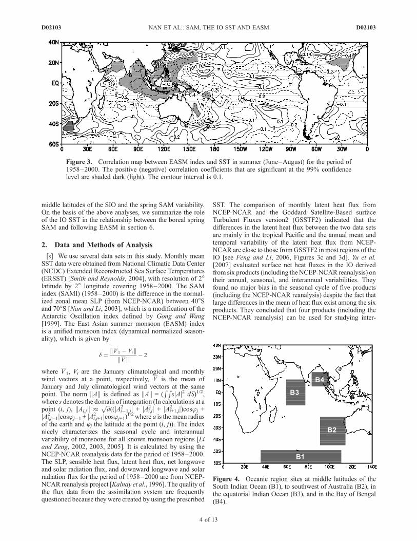
Figure 3. Correlation map between EASM index and SST in summer (June–August) for the period of1958–2000. The positive (negative) correlation coefficients that are significant at the 99% confidencelevel are shaded dark (light). The contour interval is 0.1.

Figure 4. Oceanic region sites at middle latitudes of theSouth Indian Ocean (B1), to southwest of Australia (B2), inthe equatorial Indian Ocean (B3), and in the Bay of Bengal(B4).


4 of 13

D02103

annual variability. Since other atmospheric variables used inthis paper are from NCEP-NCAR, for example SLP andEASM index, we choose to use the flux data from NCEP-NCAR reanalysis for data coherence. The boreal spring andsummer is defined as April–May and June–August,respectively.[9] Following methods are applied in this study.[10] 1. Composites[11] The composite analysis is used to examine the

variabilities of the IO SST associated with the extremeSAM events and corresponding physical processes. Thehigh and low SAMI cases were selected based on thefluctuations of the index beyond one standard deviation.The high spring SAMI cases occur in 1976, 1989, 1993,1995, 1996, 1998, 1999 and 2000, and the low spring SAMIcases occur in 1958, 1959, 1960, 1965, 1966, 1968, 1980and 1990.[12] 2. ESVD (extended singular value decomposition)[13] Singular Value Decomposition is a technique of

studying the pertinent fields of two variables. ESVD anal-ysis is an extension of SVD and may extract a propagatingphenomenon with time [Kuroda and Kodera, 2001]. In thispaper, it is employed to examine the persistence of SSTanomalies in the SIO and the appearance of SST anomaliesin the equatorial Indian Ocean and Bay of Bengal in thefollowing season.[14] 3. Simultaneous correlation and lead-lag correlation[15] The simultaneous correlation is employed to illus-

trate the relationship between the EASM and SST in theequatorial Indian Ocean and Bay of Bengal. The lead-lagcorrelations are applied to examine the potential casualrelationships between boreal spring SAM and SST anoma-lies over the subtropics and middle latitudes of the SIO as

well as SST anomalies in the equatorial Indian Ocean andBay of Bengal.[16] The Student’s t test is used to assess the statistical

significance of the results obtained from composite andcorrelation analyses unless specified.

3. Relationships Among the Boreal Spring SAM,the IO SST, and EASM

[17] Figure 1a presents the composite differences ofsimultaneous SST anomalies between the high and lowspring SAMI cases. The significant positive values coverthe midlatitude oceanic regions over 50�S–60�S and thesubtropics at 20�S–35�S. There is no significant anomaly inthe tropical Indian Ocean. In summer (Figure 1b), large-scale significant positive SST anomalies appear in theequatorial Indian Ocean and Bay of Bengal. The SSTanomalies in the tropical Indian Ocean strengthen fromspring to summer and the spring positive SST anomaliesover the subtropics and middle latitudes of the SIO persist tothe following summer. As well known, the warming trend inthe IO and the positive trend in SAM are significant in therecent decades [Bader and Latif, 2003; Hoerling et al.,2004; Thompson et al., 2000]. To isolate the contribution ofthe trends from that of natural variability, we removed boththe trends of SAM and SST, and recalculated the compositedifferences of detrended SST anomalies between the highand low detrended spring SAMI cases (figures are not

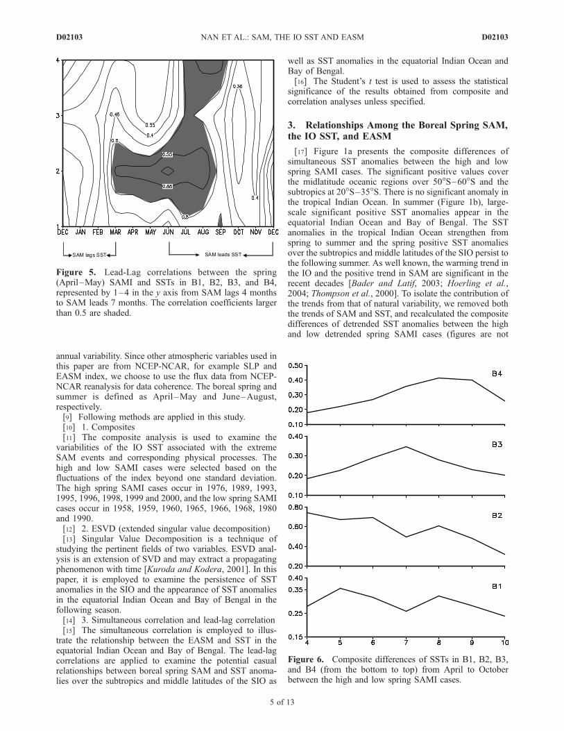
Figure 5. Lead-Lag correlations between the spring(April–May) SAMI and SSTs in B1, B2, B3, and B4,represented by 1–4 in the y axis from SAM lags 4 monthsto SAM leads 7 months. The correlation coefficients largerthan 0.5 are shaded.

Figure 6. Composite differences of SSTs in B1, B2, B3,and B4 (from the bottom to top) from April to Octoberbetween the high and low spring SAMI cases.


5 of 13

D02103

shown). After removing the linear trends, the eight highestSAMI years occur in 1961, 1962, 1964, 1976, 1979, 1989,1995 and 1999, and the eight lowest SAMI years in 1965,1966, 1968, 1980, 1981, 1986, 1990 and 1992. The generalpatterns of SST anomalies remain the same: significantlypositive SST anomalies in spring occur over the subtropicsand middle latitudes of the SIO, which persist to summer,followed by the significant positive SST anomalies in theequatorial Indian Ocean and Bay of Bengal in summer.Although after removing the linear trend, the regions withsignificant SST anomalies are reduced comparing to thosebased on the original SAMI and SST time series, thesequence of SST anomaly developments in the IO remainsthe same. Therefore both linear trends and variabilities atother timescales contribute to the connection between SAMand IO SST anomalies.[18] The variability of SST over the equatorial Pacific is

the strongest signal of interannual climate variability andexerts important impacts on the climate and environmentworldwide. We also see that negative SST anomalies in theequatorial central-eastern Pacific appear in the SST com-posite for strong positive phase of SAM in Figure 1. To sortout the relationships among SAM, ENSO and IO SST, weperformed a conditional composite analysis, which selectsthe years with extreme events of spring SAM (larger than

0.5 standard deviation of the normalized SAMI) and thenear-average spring equatorial Pacific SST (less than 0.3standard deviation of the normalized values of Nino 3.4SST (5�S–5�N, 170�W–120�W)). The high SAMI andnear-average equatorial Pacific SST conditions occur in1979 and 1996, while the low SAMI and near-averageequatorial Pacific SST conditions occur in 1959 and 1960.In the composite differences of SST between the two sets ofsamples (figures are not shown), there is no significantENSO SST pattern in the equatorial Pacific, but there aresignificant positive SST anomalies, similar to the patterns inFigure 1, occurring in the IO. That is, with near-averageequatorial Pacific SST, IO SST still responds to the extremespring SAM events. However, ENSO teleconnection tosouthern high latitudes has been well documented [Yuanand Martinson, 2001; Liu et al., 2002]. Recent studies[Zhou and Yu, 2004; Yuan and Li, 2008] showed that ENSOand SAM share large amounts of variance at interannualtimescale, which influences sea ice and SST variability inthe Antarctic. Therefore the interaction among ENSO, SAMand the IO SST needs to be further examined in the future.SAM as a midlatitude–high latitude mode likely has adirect and independent relation with the IO SST variability.[19] To further isolate the development of SST anomalies

in the IO that are associated with the spring SAM variabil-

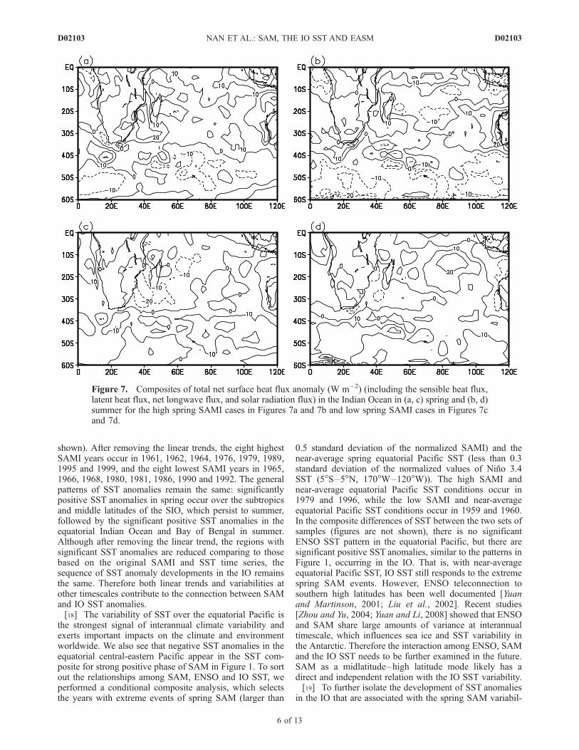
Figure 7. Composites of total net surface heat flux anomaly (W m�2) (including the sensible heat flux,latent heat flux, net longwave flux, and solar radiation flux) in the Indian Ocean in (a, c) spring and (b, d)summer for the high spring SAMI cases in Figures 7a and 7b and low spring SAMI cases in Figures 7cand 7d.


6 of 13

D02103

ity, ESVD is applied to the extratropical SH SLP anomaly inspring and SST anomaly in the IO from April to August.Figure 2 illustrates the leading mode, which accounts for60% of the total covariance between the boreal spring SLPanomalies and the combined 5-month SST anomalies. Thefirst pattern of the extratropical SH SLP accounts for 21%of its total squared covariance and the first patterns of SSTin the IO account for 19.5%, 20.4%, 22.8%, 21.2% and19.8% of their total squared covariance from April toAugust, respectively. The extratropical SH SLP is charac-terized by the feature of the positive phase of SAM withsignificant negative correlation over southern polar cap andsignificant positive correlation over SH middle latitudes.For the SST field, in April–May, significant positive valuesare mainly over the subtropics and middle latitudes of theSIO and only a small region has significant positivecorrelation in the tropical Indian Ocean. In June, the SSTanomaly pattern in the IO changes obviously: it shows thezonal belt feature and the correlation center over thesubtropics and middle latitudes the SIO moves northward.It is more important that the significant correlation region inthe equatorial Indian Ocean is expanded and the correlationcenter value increases from 0.4 in May to 0.5 in June. InJuly–August, the significant correlation region furtherextends to Bay of Bengal. In summary, when the springSAM is in its strong positive phase, positive SST anomaliesoccur over the subtropics and middle latitudes of the SIO,

which are followed by the increased SST in the equatorialIndian Ocean and Bay of Bengal in summer.[20] The above analyses endorse the hypothesis that the

spring SAM events are connected with the SST anomaliesover the subtropics and middle latitudes of the SIO andfollowed by the summertime SST anomalies in the equato-rial Indian Ocean and Bay of Bengal. An early study [Nanand Li, 2003] has suggested that the strong positive phase ofthe spring SAM is followed by the weakened EASM, andvice versa. Here we show that EASM variability is alsorelated to SST anomalies in the equatorial Indian Ocean andBay of Bengal. Figure 3 presents the correlation mapbetween the EASM index and the IO SST in summer. Theequatorial Indian Ocean, Bay of Bengal and South ChinaSea are covered by significant negative correlations, indi-cating that the weakened EASM is associated with thewarmed SST in the these regions; and vice versa. EASMcomes through a weakening process and showed an appar-ent trend in the recent decades [Chen et al., 1992]. Weremoved both the trends of the EASM index and SST andrecalculated the correlation between them (figure is notshown). The resulting correlations show the same patternsas before, although the regions with significant correlationare reduced. Therefore both linear trends and variabilities atother timescales contribute to the connection betweenEASM and SST anomalies in the equatorial Indian Ocean,Bay of Bengal and South China Sea.

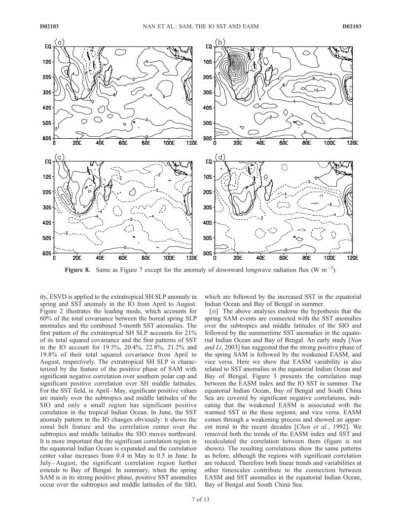
Figure 8. Same as Figure 7 except for the anomaly of downward longwave radiation flux (W m�2).


7 of 13

D02103

[21] In summary, when the spring SAM is strong positive,large-region positive anomalies of SST occur over thesubtropics and middle latitudes of the SIO, which persistfrom spring to summer. Meanwhile, a small area of positiveSST anomalies exists in the tropical Indian Ocean, which isenhanced and expanded from spring to summer. The in-creased SST in the SIO associated with the strong positiveSAM in spring seems to be followed by the increased SSTin the equatorial Indian Ocean and Bay of Bengal insummer. Furthermore, EASM is closely related to SST inthe equatorial Indian Ocean, Bay of Bengal and SouthChina Sea. When SST in these regions is above nearaverage, EASM tends to be weak. Therefore the IO SSTis associated with SAM and EASM, which plays animportant bridging role in the SAM-EASM relationship.

4. Connections Among the SSTs in DifferentRegions of the IO

[22] As presented above, SST anomalies in the IO areassociated with SAM variability in boreal spring and EASMin the following season. Here we examine how theseassociated IO SST anomalies are established and how theyevolve through these two seasons.[23] For the convenience of the study, the IO is parti-

tioned into four regions (Figure 4) based on the distributionof SST anomalies associated with the spring SAM (as

shown in Figure 1). The oceanic region at middle latitudesof the SIO is defined as the area of 36�E to 110�E inlongitudes and 50�S to 60�S in latitudes (B1); the region tothe southwest of Australia is from 92�E to 114�E inlongitudes and 22�S to 44�S in latitudes (B2); the equatorialIndian Ocean region is from 60�E to 76�E in longitudes and10�S to 10�N in latitudes (B3); Bay of Bengal region isfrom 84�E to 98�E in longitudes and 6�N to 16�N inlatitudes (B4). Each regional mean SST is used to representthe SST variability in the whole region.[24] Figure 5 shows the correlations between the spring

SAMI and the SSTs in the four oceanic regions from SAMlags 4 months to SAM leads 7 months. The lagged corre-lation coefficients (SAM lags SSTs) are much weaker thanthe leading correlation coefficients (SAM leads SSTs). Inother words, the correlation coefficients are stronger whenthe SSTs in these four oceanic regions lag spring SAMevents, suggesting that the primary process is the atmo-sphere forcing the ocean, instead of the ocean forcing theatmosphere. The high correlation coefficients in B1 and B2begin in March–May, then persist into June–August. Thesehigh correlation coefficients spread to B3 and B4 in Julyand persist through September in these regions. This revealsthat not only the SST anomalies in B1–B2 were a strongpersistence trait, but also the SST anomalies in B3–B4follow those in B1–B2 and persist through the summer too.

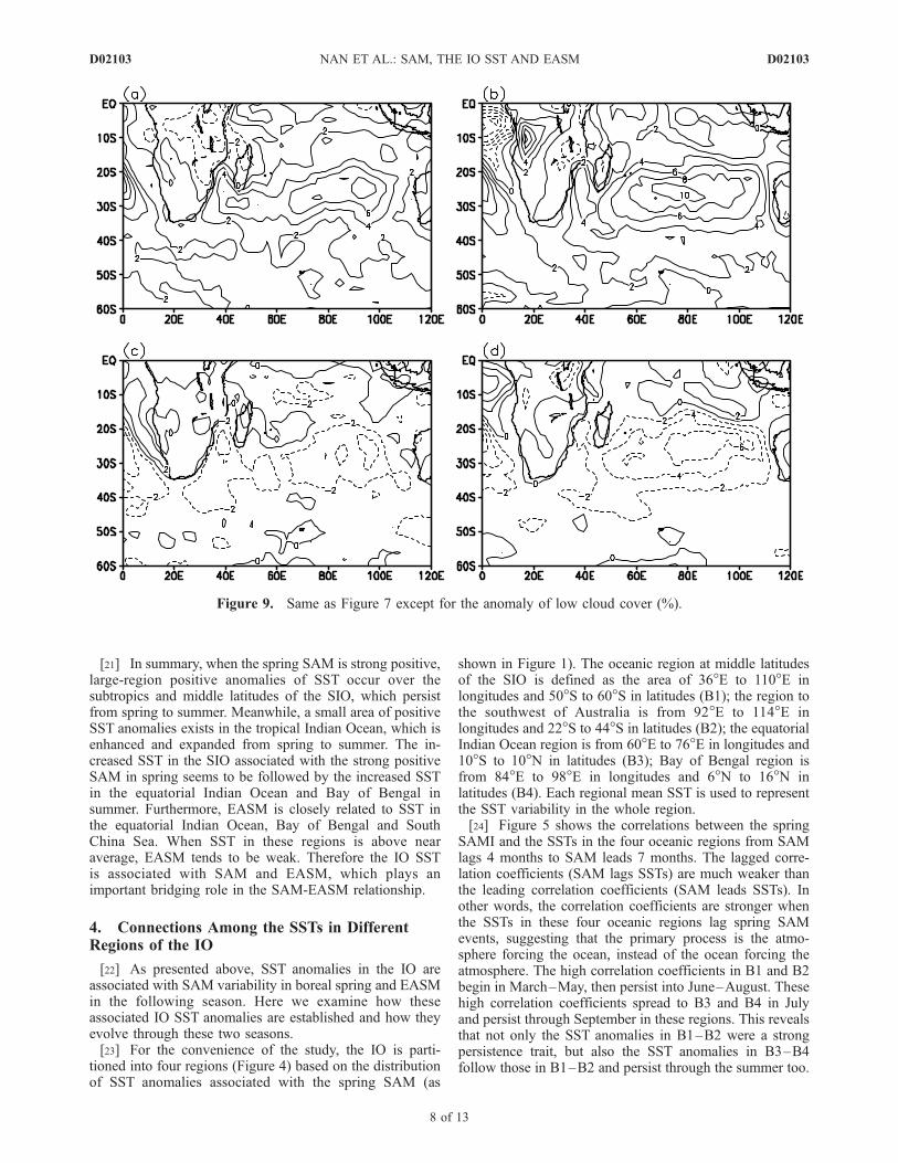
Figure 9. Same as Figure 7 except for the anomaly of low cloud cover (%).


8 of 13

D02103

[25] During the 43-a period from 1958 to 2000, thenumbers of years during which the SAMI anomaly sign issame as the SST anomaly signs in the spring are 27, 31, 26and 25 in B1, B2, B3 and B4, account for 62.8%, 72.1%,60.4% and 58.1% of the total number of years, respectively.The numbers of years during which the sign of spring SAMIanomaly is same as the sign of summer SST anomaly are 31,35, 29 and 27, respectively, account for 72.1%, 81.4%,67.4% and 62.8% of the total number of years. Thesestatistics show that following the strong positive (negative)spring SAM events, the SSTs in the four oceanic regionstend to be warmer (colder) than normal in the same seasonand the following summer. The numbers of years duringwhich the SST anomaly signs are consistent in spring andsummer are 33, 33, 34 and 35, respectively, account for76.7%, 76.7%, 79.1% and 81.2% of the total number ofyears. It also suggests that the SST anomalies in all theseregions have a strong persistence from spring to summer.[26] Figure 6 is the composite difference of SST anoma-

lies in the four oceanic regions between the high and lowspring SAMI cases from April to October. The highestanomalies in B1 and B2 are concentrated in April–Mayand the highest anomalies in B3 and B4 are in July–August.These further verified the above finding that the springSAM events has close relation to SST anomalies over the

subtropics and middle latitudes, which is followed by theSST anomalies in the equatorial Indian Ocean and Bay ofBengal.

5. Possible Physical Processes Responsible for theSST Anomaly in the SIO

[27] The above analyses show SST anomalies in the SIOare associated with SAM variability. To examine potentialphysical processes responsible for the relationship, heatfluxes at the air-sea interface and atmospheric circulationsin the SIO are analyzed.[28] Changes in the oceanic heat budget and transport are

of great importance for the understanding of global climate.In climatology, the ocean releases heat to the atmosphere inthe IO in boreal spring and summer. Figure 7 shows thecomposites of total net surface heat flux (including sensibleheat flux, latent heat flux, net longwave and solar radiationflux) anomalies for the high and low spring SAMI cases.For the net flux from NCEP-NCAR data, positive valuesmean that the ocean vents the heat to the atmosphere. Forthe high (low) SAMI cases, the anomalies of net surfaceheat flux are negative (positive) at about 50�S–60�S inspring and summer, indicating that ocean releases less(more) net heat to the atmosphere, which is consistent with

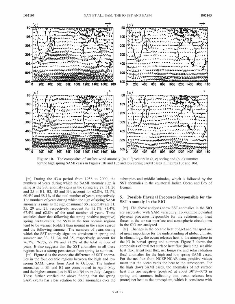
Figure 10. The composites of surface wind anomaly (m s�1) vectors in (a, c) spring and (b, d) summerfor the high spring SAMI cases in Figures 10a and 10b and low spring SAMI cases in Figures 10c and 10d.


9 of 13

D02103

the increase (decrease) of SST. Therefore the SST anomaliesat 50�S–60�S of the SIO are likely a result of responding tothe change in surface heat flux.[29] Then, we examined the anomalies of each compo-

nent of total net surface heat flux to isolate the dominantcontributor to the SST anomalies in the SIO. Among them,the longwave radiation flux seems to have such a connec-tion. The change of the net longwave radiation flux coin-cides with the SST anomalies over the subtropics of theSIO. It reflects the downward longwave radiation flux(Figure 8). For the high SAMI cases, positive anomaliesof downward longwave radiation flux are centered at 20�S–30�S with maximum of 6 W m�2 in spring and 10 W m�2 insummer, indicating the increase of the downward longwaveradiation flux (Figures 8a and 8b). The increased downwardlongwave radiation warms the sea surface. For the strongnegative SAMI cases, the negative anomalies of the down-ward longwave radiation occur in the SIO, which are centerednear 30�S with the maximum magnitude of �6 W m�2 inspring and�8 W m�2 in summer. It suggests the decrease ofdownward longwave radiation flux, in favor of the decreaseof SST (Figures 8c and 8d). The anomalies of downwardlongwave radiation flux match the SST anomalies over thesubtropics in Figure 1, suggesting its dominant contributionto the change in SST.[30] The cloud cover is an important factor influencing

the magnitude of the downward longwave radiation flux.

Figure 9 shows the composites of low cloud cover anoma-lies for the high and low SAMI cases. For the high SAMIcases, positive anomalies appear in the SIO near 20�S–30�Swith a maximum magnitude of 8% in spring and 10% insummer, indicating the increase of low cloud cover. That isconsistent with the increase of the downward longwaveradiation flux in Figures 8a and 8b. For the low SAMIcases, negative anomalies occur over the subtropics of theSIO with centers near 20�S–30�S. The magnitudes in thesecenters are �4% in spring and �6% in summer, indicatingthe decrease of the low cloud cover. The cloud may absorband reflect the solar radiation, and cool the Earth surface. Itmay also absorb and emit the longwave radiation, and warmthe Earth surface. The distributions of anomalies of the lowcloud cover and downward longwave radiation flux arematched nicely in Figures 8 and 9, suggesting the anomaliesof the low cloud cover might be the cause of the change ofdownward longwave radiation flux. The anomalies ofdownward longwave radiation are also collocated withSST anomalies in Figure 1. Therefore the low cloud mayplay a role in warming the sea surface in the subtropicsof the SIO through changing the downward longwaveradiation.[31] How does spring SAM influence the low cloud cover

over the subtropics of the SIO? Figure 10 is composites ofthe surface wind anomaly vectors for the high and lowSAMI cases. When SAM is in its strong positive phase,

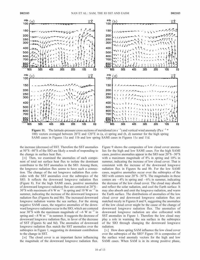
Figure 11. The latitude-pressure cross sections of meridional (m s�1) and vertical wind anomaly (Pa s�1 *100) vectors averaged between 20�E and 120�E in (a, c) spring and (b, d) summer for the high springSAMI cases in Figures 11a and 11b and low spring SAMI cases in Figures 11c and 11d.


10 of 13

D02103

subtropical highs move southward. An anomalous anticy-clone appears to the southeast of Africa near 40�S–50�Sand an anomalous cyclone occurs in the eastern SIO near20�S–30�S (Figure 10a). Accordingly, anomalous upwardmotions prevail in the middle–lower troposphere at 20�S–30�S, and anomalous downward motions at 40�S–50�S(Figure 11a), indicating that the regional Ferrel Cell weak-ens. The large-scale anomalous upward motions may causethe increase of low cloud cover and downward longwaveradiation flux. When SAM is in its strong negative phase, apair of anomalous cyclone and anticyclone dominates theregion to the southeast of Africa and the eastern IO, andthe regional Ferrel Cell strengthens (Figures 10c and 11c).The anomalous downward motions (Figure 11c) at 20�S–30�S reduce the low cloud cover and then the downwardlongwave radiation flux. In summer, the surface wind fieldsand vertical circulations are not completely symmetrical forthe high and low SAMI cases. For the low SAMI cases, thehorizontal and vertical circulations keep the features inspring (Figures 10d and 11d). For the high SAMI cases,the anomalous cyclone in the eastern SIO in spring is notapparent in summer (Figure 10b). However, it is noticedthat anomalous upward motions occur in large regions at10�S–40�S (Figure 11b). Moreover, the surface circulationsare completely different at middle-lower latitudes for thehigh and low SAMI cases. Therefore SAM variability doeschange the summer atmospheric circulations at 20�S–40�S.The change of atmospheric circulations associated with

SAM causes the anomalies of low cloud cover and down-ward longwave radiation, and then leads to the SST anoma-lies over the subtropics of the SIO.[32] The change in sensible heat flux is partly responsible

for SST anomalies in the midlatitudes of SIO at 50�S–60�S.For the high SAMI cases, negative anomalies of the sensibleheat flux cover the middle latitudes at 50�S–60�S in springand summer (Figures 12a and 12b), indicating the reducedsensible heat flux from the ocean to atmosphere. For the lowSAMI cases, reversed anomalies appear in the middlelatitudes of the SIO at 50�S–60�S, indicating the increasedsensible heat flux from the ocean to atmosphere (Figures 12cand 12d). The completely different sensible heat fluxchanges for the high and low SAMI cases imply that theSAM variability does change the sensible heat flux inmiddle latitudes of the SIO at 50�S–60�S. The reduced(enhanced) sensible heat fluxes are in favor of the increase(decrease) of SST.[33] During the strong positive SAM phase, the anoma-

lous surface atmospheric circulation shows northerly windsto the south of South Africa and Australia at 40�S–60�S(Figures 10a and 10b), which could transport more (less)warmer (colder) air from middle latitudes north of 50�S(high latitudes) into 50�S–60�S and warm the air. Thewarmed air at 50�S–60�S reduces the temperature differ-ence between the ocean and atmosphere and thus reducesthe sensible heat flux from the ocean to atmosphere,resulting in positive SST anomalies. The westerly winds

Figure 12. Same as Figure 7 except for the anomaly of sensible heat flux (W m�2).


11 of 13

D02103

strengthen at 50�S–60�S (Figure 10a). However, the in-creased wind speed isn’t consistent with the decrease of thesensible heat flux. Therefore the reduced sensible heat fluxis due to warm air advection instead of increased windspeed. During the strong negative SAM phase, anomaloussoutherly winds appear at 40�S–60�S and more (less)colder (warmer) air from high latitudes (middle latitudes,north of 50�S) comes into 50�S–60�S and cools the airin the region (Figures 10c and 10d). The temperaturedifference between the ocean and atmosphere increases,leading to the enhanced sensible heat flux from the oceanto atmosphere.[34] It is hypothesized that the positive subtropical ridge

anomalies around 40�S due to the strong SAM may allowmore solar radiation in the ocean surface. However, it is notverified in observation. In the composites of downwardsolar radiation fluxes for the high spring SAMI cases(figures are not shown), downward solar radiation fluxesare reduced over the subtropics and middle latitudes of theSIO south of 20�S for high SAMI cases, which is notconsistent with the increase of the local SST.

6. Conclusion and Discussion

[35] Using the monthly means from the NCEP-NCARreanalysis and ERSST data sets for the period of 1958–2000, we investigated the relationships among boreal springSAM, IO SST and EASM. We found that the variability ofIO SST is significantly correlated with the spring SAMevents and EASM. When the spring SAM is strong positive,SST over the subtropics and middle latitudes of the SIOincreases, which is followed by the increased SST in theequatorial Indian Ocean and Bay of Bengal in summer. Theincreased SST in the equatorial Indian Ocean and Bay ofBengal is associated with the weak EASM. Therefore the IOSST plays an important bridging role in the SAM-EASMrelationship. SAM, IO SST and EASM all showed lineartrends in the recent decades. Both linear trends and varia-bilities at other timescales contribute to the connectionsamong them. If SAM continues to increase in the future andits relationships with IO SST anomalies and EASM hold,we would expect to see weaker EASM in the future.Although this SAM, IO SST and EASM teleconnectionseems to covary with ENSO events in the tropical Pacific, italso exists without any tropical forcing. Under conditions ofnear-average SST over the equatorial central-eastern Pacific,the relationship between SAM extreme events and IO SSTanomalies remains the same. This could suggest that SAMhas independent relation to SST at lower latitudes of the IO,even though it shares significant amount of variance withENSO in the tropical Pacific.[36] The analyses of SAM and SSTs in the different

regions of the IO further indicate that SAM is closelyrelated with the IO SST anomalies, which may persist fromspring to summer. And, the SST anomalies over the sub-tropics and middle latitudes of the SIO seem to be followedby the SST anomalies in the equatorial Indian Ocean andBay of Bengal. Although the results are from simplestatistical analyses, they suggest that the IO SST plays animportant role in the SAM-EASM relationship.[37] In this study, we investigate the physical processes

that link the SAM variability with SST in the SIO. The

changes in atmospheric circulations associated with SAM’svariability and consequent changes in surface heat fluxescontribute to the SST variabilities in the SIO. When thespring SAM is in its strong positive phase, an anomalousanticyclone/cyclone pair appears to southeast of Africa andsubtropical region of the eastern IO, respectively. Theanomalous upward motions prevail in the eastern SIO andanomalous downward motions occur to the southeast ofAfrica, resulting in a weaker regional Ferrel Cell. Theweakening of the downward branch of the Ferrel Cellcauses the increase of the low cloud cover and then thedownward longwave radiation flux. In addition, west of theanomalous anticyclone to the southeast of Africa, anoma-lous northerly winds transport more warm air into 50�S–60�S, which would reduce sensible heat fluxes and conse-quently generate SST anomalies. The increased downwardlongwave radiation and reduced sensible heat are likelyresponsible for the increase of SST in the SIO.[38] In conclusion, it is air-sea interaction contributing to

the relationships among the boreal spring SAM, IO SST andEASM. The variability of IO SST might play an importantbridging role between the spring SAM and EASM. Thispaper presents a new pathway for the IO SST anomalies thatmay influence EASM.[39] In spite of the simple explanations above, some

physical processes are unclear. Through what processes dothe SST anomalies in the equatorial Indian Ocean and Bayof Bengal connect with the SST anomalies in the SIO?Could the physical processes in this study be verified innumerical experiments? We only examine the heat exchangeat the air-sea interface and the corresponding atmosphericcirculation. Other possible processes in the ocean were notanalyzed. In addition, this may be only one of manypossible pathways that relate the spring SAM to EASM.These open questions need to be examined in the future.

[40] Acknowledgments. We thank the Climate Diagnostic Center/NOAA for providing the NCEP-NCAR reanalysis data and monthly meanERSST data on its homepage. Three anonymous reviewers are thanked forthe valuable comments on the manuscript. This work was jointly sponsoredby the Chinese COPES project (GYHY200706005), 973 Program(2006CB403600), and the National Ocean and the Atmosphere Adminis-tration of USA through Grant NA030AR4320179.

ReferencesBader, J., and M. Latif (2003), The impact of decadal-scale Indian Oceansea surface temperature anomalies on Sahelian rainfall and the NorthAtlantic Oscillation, Geophys. Res. Lett., 30(22), 2169, doi:10.1029/2003GL018426.

Chen, L., M. Dong, and Y. Shao (1992), The characteristics of interannualvariations on the East Asian monsoon, J. Meteorol. Soc. Jpn., 70, 397–421.

England, M. H., C. C. Ummenhofer, and A. Santoso (2006), Interannualrainfall extremes over southwest Western Australia linked to IndianOcean climate variability, J. Clim., 19, 1948–1969.

Fauchereau, N., S. Trzaska, Y. Richard, P. Roucou, and P. Camberlin(2003), Sea-surface temperature covariability in the southern Atlanticand Indian Oceans and its connect with the atmospheric circulation inthe southern hemisphere, Int. J. Climatol., 23, 663–677.

Feng, L., and J. Li (2006), A comparison of latent heat fluxes over globaloceans for ERA and NCEP with GSSTF2, Geophys. Res. Lett., 33,L03810, doi:10.1029/2005GL024677.

Gao, H., F. Xue, and H. Wang (2003), Influence of interannual variability ofAntarctic oscillation on meiyu along the Yangtze and Huaihe River valleyand its importance to prediction, Chin. Sci. Bull., 48, 61–67.

Genthon, C., G. Krinner, and M. Sacchettini (2003), Interannual Antarctictropospheric circulation and precipitation variability, Clim. Dyn., 21,298–307, doi:10.1007/s00382-003-0329-1.


12 of 13

D02103

Gong, D. Y., and S. W. Wang (1999), Definition of Antarctic oscillationindex, Geophys. Res. Lett., 26, 459–462.

Hermes, J. C., and C. J. C. Reason (2005), Ocean model diagnosis ofinterannual coevolving SST variability in the South Indian and SouthAtlantic oceans, J. Clim., 18, 2864–2882.

Hoerling, M. P., J. W. Hurrell, T. Xu, G. T. Bates, and A. S. Phillips (2004),Twentieth century North Atlantic climate change. part II: Understandingthe effect of Indian Ocean warming, Clim. Dyn., 23, 391 – 405,doi:10.1007/s00382-004-0433-x.

Kalnay, E., et al. (1996), The NCEP/NCAR 40-year reanalysis project, Bull.Am. Meteorol. Soc., 77, 437–471.

Kidson, J. W. (1975), Eigenvector analysis of monthly mean surface data,Mon. Weather Rev., 103, 182–186.

Klein, S. A., B. J. Soden, and N. C. Lau (1999), Remote sea surfacetemperature variations during ENSO: Evidence for a tropical atmosphericbridge, J. Clim., 12(4), 917–932.

Kucharski, F., F. Molteni, and J. H. Yoo (2006), SST forcing of decadalIndian monsoon rainfall variability, Geophys. Res. Lett., 33, L03709,doi:10.1029/2005GL025371.

Kuroda, Y., and K. Kodera (2001), Variability of the polar night jet in theNorthern and Southern hemispheres, J. Geophys. Res., 106, 20,703–20,713.

Li, J. P., and Q. C. Zeng (2002), A unified monsoon index, Geophys. Res.Lett., 29(8), 1274, doi:10.1029/2001GL013874.

Li, J. P., and Q. C. Zeng (2003), A new monsoon index and the geogra-phical distribution of the global monsoons, Adv. Atmos. Sci., 20, 299–302.

Li, J. P., and Q. C. Zeng (2005), A new monsoon index, its interannualvariability and relation with monsoon precipitation (in Chinese), Clim.Environ. Res., 10(3), 351–365.

Liu, J., X. Yuan, D. Rind, and D. G. Martinson (2002), Mechanism study ofthe ENSO and southern high latitude climate teleconnections, Geophys.Res. Lett., 29(14), 1679, doi:10.1029/2002GL015143.

Nan, S. L., and J. P. Li (2003), The relationship between the summerprecipitation in the Yangtze River valley and the boreal spring SouthernHemisphere Annular Mode, Geophys. Res. Lett., 30(24), 2266,doi:10.1029/2003GL018381.

Reason, C. J. C., and M. Rouault (2005), Links between the AntarcticOscillation and winter rainfall over western South Africa, Geophys.Res. Lett., 32, L07705, doi:10.1029/2005GL022419.

Reason, C. J. C., R. J. Allan, J. A. Lindesay, and T. J. Ansell (2000), ENSOand climatic signals across the Indian Ocean Basin in the global context.part 1: Interannual composite patterns, Int. J. Climatol., 20, 1285–1327.

Rogers, J. R., and H. van Loon (1982), Spatial variability of sea levelpressure and 500 mb height anomalies over the Southern Hemisphere,Mon. Weather Rev., 110, 1375–1392.

Silvestri, G. E., and C. S. Vera (2003), Antarctic oscillation signal onprecipitation anomalies over southeastern South America, Geophys.Res. Lett., 30(21), 2115, doi:10.1029/2003GL018277.

Smith, T. M., and R. W. Reynolds (2004), Improved extended reconstruc-tion of SST (1854–1997), J. Clim., 17(6), 2466–2477.

Terray, P., P. Delecluse, S. Labattu, and L. Terray (2003), Sea surfacetemperature associations with the late Indian summer monsoon, Clim.Dyn., 21, 593–618.

Terray, P., S. Dominiak, and P. Delecluse (2005), Role of the southernIndian Ocean in the transitions of the monsoon-ENSO system duringrecent decades, Clim. Dyn., 24, 169–195.

Thompson, D. W. J., and J. M. Wallace (2000), Annular modes in theextratropical circulation. part I: Month-to-month variability, J. Clim.,13, 1000–1016.

Thompson, D. W. J., J. M. Wallace, and G. C. Hegerl (2000), Annularmodes in the extratropical circulation. part II: Trends, J. Clim., 13,1018–1036.

Ummenhofer, C. C., A. S. Gupta, M. J. Pook, and M. H. England (2008),Anomalous rainfall over southwest Western Australia forced by IndianOcean sea surface temperatures, J. Clim., 21, 5113–5134.

Van den Broeke, M. R., and N. P. M. Van Lipzig (2002), Impact of polarvortex variability on the wintertime low-level climate of East Antarctica:Results of a regional climate model, Tellus, 54, 485–496.

Watterson, I. G. (2000), Southern midlatitude zonal wind vacillation and itsinteraction with the ocean in GCM simulations, J. Clim., 13, 562–578.

Yu, L., X. Jin, and R. A. Weller (2007), Annual, seasonal, and interannualvariability of air-sea heat fluxes in the Indian Ocean, J. Clim., 20, 3190–3209.

Yuan, X., and D. G. Martinson (2001), The Antarctic dipole and its pre-dictability, Geophys. Res. Lett., 28, 3609–3612.

Yuan, X., and C. Li (2008), Climate modes in southern high latitudes andtheir impacts on Antarctic sea ice, J. Geophys. Res., 113, C06S91,doi:10.1029/2006JC004067.

Zhou, T., and R. Yu (2004), Sea-surface temperature induced variability ofthe Southern Annular Mode in an atmospheric general circulation model,Geophys. Res. Lett., 31, L24206, doi:10.1029/2004GL021473.

Zhu, Y. L., and D. D. Houghton (1996), The impact of Indian Ocean SSTon the large-scale Asian summer monsoon and the hydrological cycle,Int. J. Climatol., 16, 617–632.

��J. Li, National Key Laboratory of Numerical Modeling for Atmospheric

Sciences and Geophysical Fluid Dynamics, Institute of AtmosphericPhysics, Chinese Academy of Sciences, P.O. Box 9804, Beijing 100029,China. ([email protected])S. Nan and P. Zhao, Chinese Academy of Meteorological Sciences,

No. 46, Zhongguancun Nandajie, Haidian District, Beijing 100081, China.X. Yuan, Lamont-Doherty Earth Observatory, Columbia University, 61

Route 9W, Palisades, NY 10964, USA.


13 of 13

D02103

boreal spring southern hemisphere annular mode, indian

Documents