Copyright Warning & Restrictions

The copyright law of the United States (Title 17, UnitedStates Code) governs the making of photocopies or other

reproductions of copyrighted material.

Under certain conditions specified in the law, libraries andarchives are authorized to furnish a photocopy or other

reproduction. One of these specified conditions is that thephotocopy or reproduction is not to be “used for any

purpose other than private study, scholarship, or research.”If a, user makes a request for, or later uses, a photocopy orreproduction for purposes in excess of “fair use” that user

may be liable for copyright infringement,

This institution reserves the right to refuse to accept acopying order if, in its judgment, fulfillment of the order

would involve violation of copyright law.

Please Note: The author retains the copyright while theNew Jersey Institute of Technology reserves the right to

distribute this thesis or dissertation

Printing note: If you do not wish to print this page, then select“Pages from: first page # to: last page #” on the print dialog screen

The Van Houten library has removed some ofthe personal information and all signatures fromthe approval page and biographical sketches oftheses and dissertations in order to protect theidentity of NJIT graduates and faculty.

ABSTRACT

BOOTSTRAPPING TSMARS MODELS

byLiangzhong Chen

We investigate bootstrap inference methods for nonlinear time series models

obtained using Multivariate Adaptive Regression Splines for Time Series (TSMARS),

for which theoretical properties are not currently known. We use two different

methods of bootstrapping to obtain confidence intervals for the underlying nonlinear

function and prediction intervals for future values, based on estimated TSMARS

models for the bootstrapped data. We also explore the method of Bootstrap

AGGregatING (Bagging), due to Breiman (1996), to investigate whether the

residual and prediction mean squared errors from a fitted TSMARS model can be

reduced by averaging across the values obtained from each of the bootstrapped

models. We find that, although the estimated parameters of models obtained using

TSMARS may differ markedly from one bootstrap replicate to another, fitted values

from the estimated models are relatively stable. We also find that Bagging can lead

to smaller residual and forecasts errors, but that confidence and prediction intervals

based on bootstrapping have a coverage that is much too small.

Key Words: Bootstrapping; Multivariate Adaptive Regression Splines; Nonlinear

time series; TSMARS

BOOTSTRAPPING TSMARS MODELS

byLiangzhong Chen

A ThesisSubmitted to the Faculty of

New Jersey Institute of Technologyin Partial Fulfillment of the Requirements for the Degree of

Master of Science in Applied Mathematics

Department of Mathematical Sciences

May 1998

APPROVAL PAGE

BOOTSTRAPPING TSMARS MODELS

Liangzhong Chen

bonnie K. Ray, Thesis Advisor 7 Date "-Associate Professor of Mathematical Sciences, NJIT

Manish C. Bhattacharjee, Committee Member DateProfessor of Mathematical Sciences, NJIT

John Bechtold, Committee Member DateAssociate Professor of Mathematical Sciences, NJIT

BIOGRAPHICAL SKETCH

Author: Liangzhong Chen

Degree: Master of Science

Date: May 1998

Undergraduate and Graduate Education:

• Master of Science in Mathematical Sciences,New Jersey Institute of Technology, Newark, NJ, 1998

• Bachelor of Science in Mathematical Sciences,Peking University, Beijing, P.R. China, 1992

Major: Applied Mathematics

To my beloved family

ACKNOWLEDGMENT

The research of Liangzhong Chen was completed as part of his master's thesis

under the direction of Prof. Bonnie Ray. The research of Bonnie Ray was supported

in part by National Science Foundation Grant DMS-9623884 and the Department of

Mathematical Sciences, the New Jersey Institute of Technology. The author wish to

thank Prof. James Ramsey and Prof. Upmanu La11 for helpful discussions.

vi

TABLE OF CONTENTS

Chapter Page

1 INTRODUCTION 1

2 THE TSMARS METHODOLOGY 3

2.1 The Algorithm 3

2.2 Forecasting with ASTAR Models 6

2.3 Parameters of the TSMARS Algorithm 7

3 BOOTSTRAPPING NONLINEAR TIME SERIES 9

3.1 Residual-based Bootstrapping 9

3.2 Regression-based Bootstrapping 11

3.3 Bagging Predictors 11

4 A SIMULATION STUDY 13

4.1 A Simple ASTAR Model 13

4.2 An ASTAR Model with Interactions 20

5 AN APPLICATION 24

6 DISCUSSION 30

vii

LIST OF TABLES

Table Page

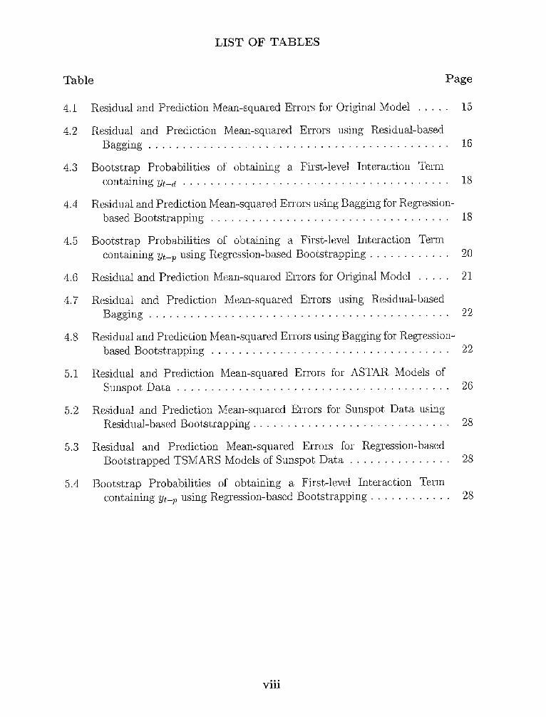
4.1 Residual and Prediction Mean-squared Errors for Original Model 15

4.2 Residual and Prediction Mean-squared Errors using Residual-basedBagging 16

4.3 Bootstrap Probabilities of obtaining a First-level Interaction Term

containing yt-d 18

4.4 Residual and Prediction Mean-squared Errors using Bagging for Regression-based Bootstrapping 18

4.5 Bootstrap Probabilities of obtaining a First-level Interaction Termcontaining yt-p using Regression-based Bootstrapping 20

4.6 Residual and Prediction Mean-squared Errors for Original Model . . . . 21

4.7 Residual and Prediction Mean-squared Errors using Residual-basedBagging 22

4.8 Residual and Prediction Mean-squared Errors using Bagging for Regression-based Bootstrapping 22

5.1 Residual and Prediction Mean-squared Errors for ASTAR Models of

Sunspot Data 26

5.2 Residual and Prediction Mean-squared Errors for Sunspot Data usingResidual-based Bootstrapping 28

5.3 Residual and Prediction Mean-squared Errors for Regression-basedBootstrapped TSMARS Models of Sunspot Data 28

5.4 Bootstrap Probabilities of obtaining a First-level Interaction Termcontaining yt-p using Regression-based Bootstrapping 28

viii

LIST OF FIGURES

Figure Page

4.1 Simulated Data from Model (6) 14

4.2 90% Pointwise Confidence and Prediction Intervals for Simulated Datafrom Model (6) obtained using Residual-based Bootstrapping 17

4.3 90% Pointwise Regression-based Bootstrap Confidence and PredictionIntervals for Series Generated from Model (6) 19

4.4 Simulated Data from ASTAR Model (9) 21

5.1 90% Confidence and Prediction Bounds for Sunspot Data using Regression-based Bootstrapping 25

5.2 Fitted Values from Original and Bagged Models for Sunspot Dataselected using Span 9 and MSC=SC 26

5.3 Yearly Wolf Sunspot Numbers, 1700-1920 27

ix

CHAPTER 1

INTRODUCTION

Nonlinear time series models have been used extensively in recent years to model

complex dynamics that cannot be adequately represented using a linear model. One

of the techniques that has been used to approximate such complex structure is the

method of Multivariate Adaptive Regression Splines for Time Series (TSMARS).

TSMARS is based on the MARS algorithm of Friedman (1991), originally introduced

as a way to estimate nonlinear regression functions in a computationally efficient

manner using a modified recursive partitioning algorithm. Lewis and Stevens (1991)

introduced the use of MARS for modeling a time series, {10, by letting lagged values

of the series, y t-j , serve as predictor variables in the MARS algorithm, analogous

to linear autoregressive modeling. The models obtained from this procedure are

called Adaptive Spline Threshold AutoRegressive (ASTAR) time series models, and

are generalizations of the Threshold AR models of Tong (1983). Since their intro-

duction, they have been used to model time series data in such diverse fields as

oceanography (Lewis and Ray; 1997), hydrology (La11 and Moon; 1996) and finance

(De Gooijer, Ray, and Krager; 1998). A drawback to their use, however, is the lack

of knowledge regarding the properties of the estimated models. Dennison and Mallik

(1997) describe a Bayesian version of the MARS algorithm, which provides posterior

probabilities for each of the possible model terms. Their implementation does not

provide information useful for obtaining posterior distributions of fitted values or

predictions, however.

In this paper, we investigate the variability of estimated ASTAR models by

the bootstrap method. Franke, Kreiss, and Mammen (1997) showed that certain

bootstrap methods are valid for estimating the distribution of a simple nonlinear

autoregression function obtained using kernel smoothing methods. Neumann and

2

Kreiss (1997) used a wild bootstrap procedure to obtain confidence bands for

nonlinear autoregressive functions estimated using local polynomial estimation. Here

we investigate empirically the validity of two bootstrap methods for constructing

confidence and prediction bands for nonlinear autoregressive functions and futures

values and study the effect on prediction accuracy of using averaged bootstrap

replicates for forecasting. Additionally, we attempt to investigate the bootstrap

distributions of estimated parameters in an ASTAR model. The rest of the paper is

organized as follows. In chapter 2, we provide a brief introduction to the TSMARS

algorithm. chapter 3 discusses 2 methods for bootstrapping ASTAR models and the

technique of Bootstrap AGGregatING (Bagging), introduced by Brennan (1996).

chapter 4 gives results of a small simulation study, while chapter 5 gives results for

a data example. chapter 6 concludes.

CHAPTER 2

THE TSMARS METHODOLOGY

Although nonparametric modeling does not require an explicit model, the TSMARS

methodology is probably best understood through introducing the following setup.

Let {yt} be a univariate time series variable that depends on d, (d > 0) past values

of y t . Assume that there are N observations on {yt} and that the data is presumed

to be described by the time series model

yt f ( 1 , yt-1 , • • yt - d) + Et (2.1)

over some domain D C Rn, (n. = 2 + d), which contains the data. Here, 1 denotes

a model constant, f(.) is a measurable function from R." to R. that reflects the

true but unknown relationship between y t and (y t-1 , y t- d ) and єt NID(0,

The goal is to construct a function(1f(1, yt-1,. • • ,yt-d) that can serve as a reasonable

approximation to f(1, y t-1, • • • ,yt-d) over the domain D.

2.1 The Algorithm

Within the above context, MARS can be viewed as a generalization of the recursive

partitioning regression strategy of Morgan and Sonquist (1963) and Breiman,

Friedman, Olshen and Stone (1984) that uses spline fitting rather than other simple

fitting functions. Let {Rj}s j=1 be a set of S disjoint subregions representing a

partitioning of D. Given these subregions, recursive partitioning approximates the

unknown function f (w t ) at wt = (1, y t-1 y t- d ) in terms of basis functions B j (w t )

so that

where B(w) = /{w t E Ri} and I{.} is an indicator function having a value one

if to t e Rj (j = 1 ) ... S) and zero otherwise. Each indicator function, in turn, is a

3

4

product of Heaviside or step functions: H(z) = 1, z > 0; H(z) = 0, z < 0, describing

each subregion R. The functions { (wt are generally taken to be of quite

simple form. The most common is a constant function, i.e. f (wt ) = cj Vwt E Rj

(Breiman et al., 1984). The aim is to use the data to simultaneously estimate a good

set of subregions, without enforcing continuity at the boundaries, and the parameters

associated with the separate basis functions in each subregion.

The recursive partitioning follows a two-step procedure. Starting from the

entire domain R 1 D, all existing subregions (parent) are each recursively split

into two sibling subregions. The split is jointly optimized over all variables and all

observed values using a goodness-of-fit criterion on the resulting approximation f(.)

to f(.). This is continued iteratively until a large number of disjoint subregions

{Rj}M j=2, for some prespecified M > S, are generated. This is called the forward

step. In the second, or backward, step the subregions are recombined in a reverse

manner until a good set of nonoverlapping subregions is obtained, using a criterion

that penalizes both for lack-of-fit and increasing number of regions.

As pointed out by Friedman (1991) and Lewis and Stevens (1991), several

problems are associated with the above recursive scheme. In Friedman's (1991)

MARS methodology the following two important innovations are introduced. First,

to overcome the difficulty in fitting simple smooth functions, Friedman proposed

not to automatically eliminate the parent region R j during the creation of its

sibling subregions. In subsequent iterations both the parent and its corresponding

subregions are eligible for further partitioning. Also, each parent region may have

more than two sets of sibling subregions. Thus one obtains overlapping subregions

of the domain D. This allows for much greater flexibility. The second contribution

is to replace Bj(wt ) by products of linear (q=1) or cubic (q = 3) left- and right-

truncated regression splines to eliminate discontinuities at the boundaries of adjacent

subregions.

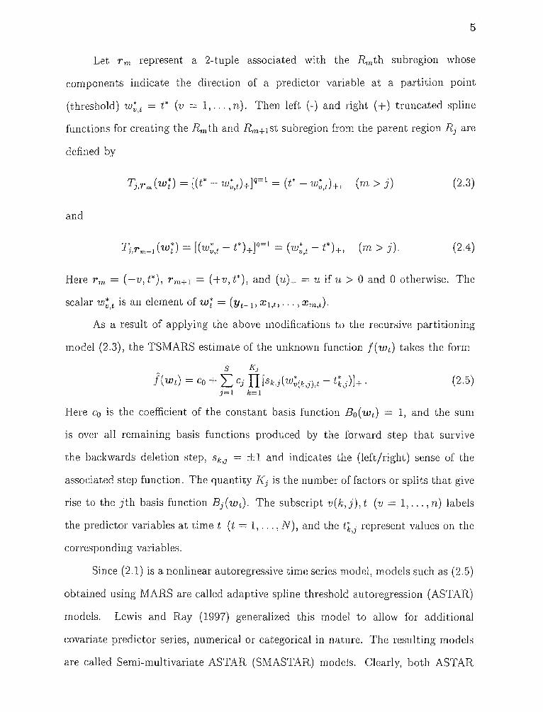
Let r, represent a 2-tuple associated with the R in d' subregion whose

components indicate the direction of a predictor variable at a partition point

(threshold) w*v,t = t* (v = 1, ... , n). Then left (-) and right (+) truncated spline

functions for creating the Rmth and Rm+1st subregion from the parent region Rj are

defined by

(2.3)

(2.4)

Here T., ( — v, t*), = (+v, t*), and (u) ± = u if u > 0 and 0 otherwise. The

scalar w*v,t is an element of w t* = (y t-1 , x, • • , xm,t).

As a result of applying the above modifications to the recursive partitioning

model (2.3), the TSMARS estimate of the unknown function f (w t ) takes the form

(2.5)

Here c0 is the coefficient of the constant basis function B0(wt ) = 1, and the sum

is over all remaining basis functions produced by the forward step that survive

the backwards deletion step, sk,j = ±1 and indicates the (left/right) sense of the

associated step function. The quantity K j is the number of factors or splits that give

rise to the jth basis function Bj(wt ). The subscript v(k, j), t (v = 1, , n) labels

the predictor variables at time t (t = 1, N), and the t represent values on the

corresponding variables.

Since (2.1) is a nonlinear autoregressive time series model, models such as (2.5)

obtained using MARS are called adaptive spline threshold autoregression (ASTAR)

models. Lewis and Ray (1997) generalized this model to allow for additional

covariate predictor series, numerical or categorical in nature. The resulting models

are called Semi-multivariate ASTAR (SMASTAR) models. Clearly, both ASTAR

6

and SMASTAR models are more general than, respectively, the SETAR and the

self-exciting open-loop threshold autoregressive (TARSO) models of Tong (1990).

These latter models identify piecewise linear functions over disjoint subregions,

which are discontinuous at their boundaries of the domain D of interest. In contrast,

the TSMARS methodology derives nonlinear threshold models that are continuous

in the domain of the predictor variables. Moreover, in Tong's SETAR and TARSO

approach interactions among lagged predictor variables (if present) are not allowed,

whereas this is not the case with TSMARS.

2.2 Forecasting with ASTAR Models

Forecasts for ASTAR models may be obtained in two ways—iteratively or directly.

Given yt, ..., an iterated forecast of y t+k , k > 1 is computed as yt+k

f(yt+k-1,•••,yt+k-d), where j = yj when j < 0. The forecasts are computed

iteratively beginning yt+1•

A direct forecast of yt+k is computed directly from yt , .An ASTAR

model for {yt} is obtained using only values of the series at lags greater than or

equal to k as predictors, e.g. f(yt+k-k,···, yt+k-d). When this setup is used,

the final model is selected so that it minimizes a function of the in-sample k-step

prediction error, as opposed to the model obtained for iterated forecasting, which is

optimized for one-step-prediction. A disadvantage of the direct forecasting method is

that a different model must be fit for each value of k. In this paper, we concentrate on

iterative forecasting, as bootstrapping the estimated direct forecast model for several

values of k is more computationally intensive. Of course, if the "correct" model

is known, estimation of model parameters to minimize one-step-ahead prediction

results in optimal predictions at all forecast steps. However, the TSMARS algorithm

is used to obtain only an approximation to the underlying dynamical structure, thus

the method of direct forecasting may provide better forecasts in this framework.

7

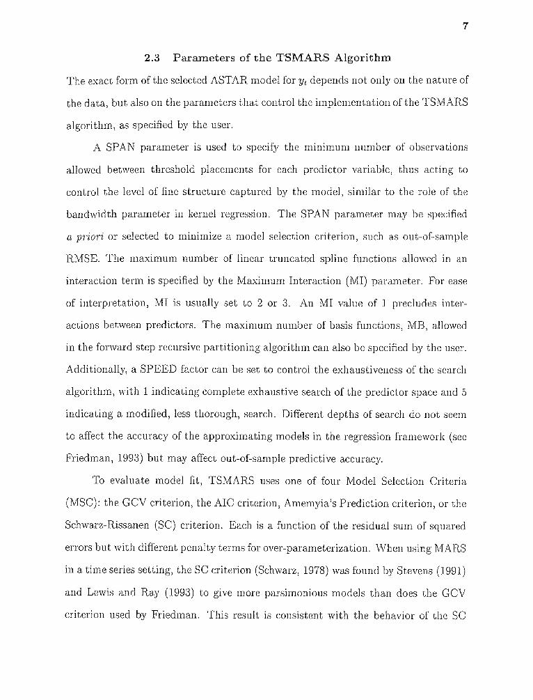
2.3 Parameters of the TSMARS Algorithm

The exact form of the selected ASTAR model for y t depends not only on the nature of

the data, but also on the parameters that control the implementation of the TSMARS

algorithm, as specified by the user.

A SPAN parameter is used to specify the minimum number of observations

allowed between threshold placements for each predictor variable, thus acting to

control the level of fine structure captured by the model, similar to the role of the

bandwidth parameter in kernel regression. The SPAN parameter may be specified

a priori or selected to minimize a model selection criterion, such as out-of-sample

RMSE. The maximum number of linear truncated spline functions allowed in an

interaction term is specified by the Maximum Interaction (MI) parameter. For ease

of interpretation, MI is usually set to 2 or 3. An MI value of 1 precludes inter-

actions between predictors. The maximum number of basis functions, MB, allowed

in the forward step recursive partitioning algorithm can also be specified by the user.

Additionally, a SPEED factor can be set to control the exhaustiveness of the search

algorithm, with 1 indicating complete exhaustive search of the predictor space and 5

indicating a modified, less thorough, search. Different depths of search do not seem

to affect the accuracy of the approximating models in the regression framework (see

Friedman, 1993) but may affect out-of-sample predictive accuracy.

To evaluate model fit, TSMARS uses one of four Model Selection Criteria

(MSC): the GCV criterion, the AIC criterion, Amemyia's Prediction criterion, or the

Schwarz-Rissanen (SC) criterion. Each is a function of the residual sum of squared

errors but with different penalty terms for over-parameterization. When using MARS

in a time series setting, the SC criterion (Schwarz, 1978) was found by Stevens (1991)

and Lewis and Ray (1993) to give more parsimonious models than does the GCV

criterion used by Friedman. This result is consistent with the behavior of the SC

8

criterion when selecting among linear ARMA(p, q) models, as the SC penalizes for

heavily for additional model parameters than do the other criteria.

In our simulation study, we investigate the effects of the SPAN and MSC

parameters on the variability of the fitted models. The SPEED parameter is always

set to one, indicating complete exhaustive search. The MB parameter is chosen as

a function of 71, the number of time series observations. We use MI < 3, for more

interpretable models.

CHAPTER 3

BOOTSTRAPPING NONLINEAR TIME SERIES

Bootstrapping time series has been an area of much research in recent years.

Initial research focused on parametric residual-based resampling procedures (see, for

example, Chatterjee (1986) for a discussion of bootstrapping ARMA(p, q) models

and Stine (1987) regarding AR(p) models), while more recent research has looked at

nonparametric techniques for generating time series having the same structure as the

original using, for instance, block resampling (Künsch, 1989; Liu and Singh, 1992).

Berkowitz and Killian (1996) give a review of the different methods available for

bootstrapping time series, concentrating on techniques applicable to linear processes.

Bootstrap results for nonlinear time series models have only recently begun to be

investigated. Franke, Kreiss, and Mammen (1997) discuss the bootstrap for kernel

smoothed estimates of nonlinear autoregressive functions, while Neumann and

Kreiss (1997) discuss bootstrap confidence bounds for nonlinear functions estimated

using local polynomial smoothing. In this paper, we investigate empirically two

methods for bootstrapping nonlinear autoregressive time series models obtained

using TSMARS: (1) a parametric, residual-based bootstrap approach and (2) a

nonparametric, regression-based bootstrap.

3.1 Residual-based Bootstrapping

Let y t = f(t - 1, • ..,yt - d) + et. As discussed in chapter 2, an estimate of P.),

denoted by P.), can be obtained using the TSMARS algorithm. Let Et =

f (yt - 1, • • • Yd). Assuming e t are approximately independent and identically

distributed, i.e. I(-) approximates the structure of f(-) fairly well, bootstrap

samples of yt may be obtained by resampling with replacement from e t and setting

Yt,b f(yt - 1,•••, yt - d)+ єt,b,t = d + 1, . . . , n, where yt,b denotes the W' bootstrap

9

10

sample, b 1, . . , B. The boot-strap samples are used to obtain B additional

estimates of f(). The bootstrap estimates can be used to form confidence intervals

on prediction intervals on y t+ . k , etc. Following Franke, Kreiss, and

Mammen (1997), only the responses y t , t = d + 1, . , n are altered when applying the

TSMARS algorithm to the bootstrapped data; the predictor variables y, , yt- d

are left unchanged from the original data. This may be thought of analogous to a

fixed design in nonparametric regression.

Franke, Kreiss, and Mammen (1997) show that, under some general strong

mixing conditions on the process {y t } and Lipschitz continuity conditions on f (•),

residual-based bootstrap estimates of f(-) obtained using kernel smoothing have

distribution converging to that of the original estimate of the nonlinear autore-

gression function when d = 1. They find that the bandwidth used in the kernel

regression for the original data must be smaller than that for the bootstrapped data,

to minimize the bias in the estimated f(). We investigate empirically whether their

results hold for nonparametric estimates of autoregression functions obtained using

TSMARS, allowing for d > 1. Following their findings for the simple case, we use

a small SPAN parameter to estimate f() for the original data, and a larger SPAN

parameter for the bootstrapped data. The motivation for this comes from results in

nonparametric regression, where it is known that using a small bandwidth reduces

the bias in the estimated regression function, but increases variability. Since our

bootstrapped samples are based on the initial estimate of f(.), we would like for

this estimate to have small bias (thus a small SPAN parameter is used), whereas we

desire the bootstrapped estimates to have smaller variability (thus a larger SPAN is

used).

11

3.2 Regression-based Bootstrapping

The bootstrapped data obtained using residual-based bootstrapping are largely

dependent on the initial estimate of f(), thus bias in this estimate will carry

over to the bootstrapped estimates. To mitigate this influence, we also consider a

nonparametric method of bootstrapping. Let (yt , xt ) denote a pair of observed data

points, where xt = (Yt-1, • • • Yt-d). Assuming the pairs (y t ,x t ) are independent

and identically distributed according to the stationary distribution of the vector

(Pt, , • • • , we can resample from the set (y e , x t ), t = d + 1, • • • , n to obtain

bootstrapped pairs with which to estimate f (•) . Note that in this context, the time

index t has no meaning, in the sense that the bootstrapped observations (yt,b, xt,b)

are reshuffled versions of (y t , xt ). Iterative forecasts of the y t process are obtained

for the regression-based bootstrapped models as for the residual-based bootstrapped

models, i.e. to forecast yn+k conditional on hi • • • ,yn+1-d), the original data

values (7] yn, • are used as the initial predictor values and forecasts obtained

iteratively using the bootstrapped estimate of f

In chapter 4, we compare the two methods of bootstrapping on the basis of

their mean-squared residual and prediction errors, as well as on the coverage of

the bootstrap confidence intervals, for simulated data. For mean-squared error

comparisons, we employ the method of Bootstrap AGGregatING (BAGGING),

described below.

3.3 Bagging Predictors

Bagging predictors is a method for generating multiple versions of a predictor

using bootstrap methods and using these to get an aggregated predictor. Breiman

(1996) showed that bagging can give substantial gains in accuracy, with actual gains

dependent on the instability of the prediction method. For ASTAR models, bagging

implies using as an estimate of yt the average of yt,b = fb (y t - 1 , — • , y t- a ), where

12

fb (.) denotes the ASTAR model for the bth bootstrapped data set and the average

is over all bootstrapped models b, b = 1, • • • , B. Thus biased estimates of f() are

pulled in towards the center of the distribution of estimates, resulting in more stable

predictions.

CHAPTER 4

A SIMULATION STUDY

To investigate the reliability of inferences obtained using bootstrapping, we conducted

a small simulation study using two different ASTAR models.

4.1 A Simple ASTAR Model

First we generated a series of length n = 312 data from the following model:

yt = 1.0 + 0.5(y ' — + 0.5(1.0 — yt-1)+1 + єts (4.1)

where Et are i.i.d. standard Normal random variables. This is a very simple ASTAR

model which is continuous at the boundary of the two prediction regions (y t- 1 < 1.0

and yt - 1 > 1.0). We expect that the TSMARS algorithm should be able to "find"

the underlying nonlinear relationship between y t and yt - 1 for this process. The data

was simulated by generating initial value y o = 1.0 + є0 and using this initial value to

generate y t , t = 1, • • • ,n recursively. Effects of the initial condition were mitigated by

generating n* = 412 values and using only the last n = 312 for analysis. Figure 4.1

shows a time series plot of the simulated series, along with a scatter plot of y t versus

yt- 1. The change in behavior when yt- 1is above or below one is evident, although

the behavior is quite noisy.

We used n o = 300 observations for model fitting and used the remaining

n, = 12 observations for forecast evaluation. These values were chosen because

they correspond to forecasting monthly data one year ahead using information from

the past 25 years, which is common for data seen in many economic and financial

applications. We allowed up to d 6 possible predictors in the estimated model,

with interactions up to level MI = 2. The number of basis functions allowed in the

forward steps of the algorithm was MB = 30. We let d = 6 in order to see how well

TSMARS is able to correctly select the true number of lagged variables in the model

13

Simulated Sin: ASTAR Model (6)

14

L

Figure 4.1 Simulated Data from Model (6)

when d > p 1. Masaratto (1990) discusses the use of the bootstrap algorithm

to reflect the true sampling uncertainty of the lag order estimate for linear AR(p)

models. We let MI =2 to see if the algorithm correctly discards potential prediction

regions distinguished by interactions between lagged variables. Various values of the

SPAN and MSC parameters were used, in order to investigate the effect of these

values on the resulting models.

As an example, the following model was obtained for the simulated data using

SPAN = 5, MSC = AIC.

We see that the constant and the coefficient and threshold values for the first term

of the true model are estimated quite accurately, however the behavior of yt in the

15

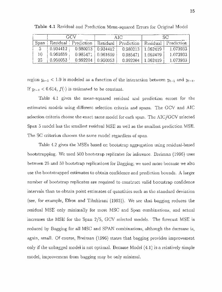
Table 4.1 Residual and Prediction Mean-squared Errors for Original Model

region yt - 1 < 1.0 is modeled as a function of the interaction between y t - 1 and y t-4 .

If yt - 4 < 0.614, f() is estimated to be constant.

Table 4.1 gives the mean-squared residual and prediction errors for the

estimated models using different selection criteria and spans. The GCV and AIC

selection criteria choose the exact same model for each span. The AIC/GCV selected

Span 5 model has the smallest residual MSE as well as the smallest prediction MSE.

The SC criterion chooses the same model regardless of span.

Table 4.2 gives the MSEs based on bootstrap aggregation using residual-based

bootstrapping. We used 500 bootstrap replicates for inference. Breiman (1996) uses

between 25 and 50 bootstrap replications for Bagging; we used more because we also

use the bootstrapped estimates to obtain confidence and prediction bounds. A larger

number of bootstrap replicates are required to construct valid bootstrap confidence

intervals than to obtain point estimates of quantities such as the standard deviation

(see, for example, Efron and Tibshirani (1993)). We see that bagging reduces the

residual MSE only minimally for most MSC and Span combinations, and actual

increases the MSE for the Span 2/5, GCV selected models. The forecast MSE is

reduced by Bagging for all MSC and SPAN combinations, although the decrease is,

again, small. Of course, Breiman (1996) states that bagging provides improvement

only if the unbagged model is not optimal. Because Model (4.1) is a relatively simple

model, improvement from bagging may be only minimal.

16

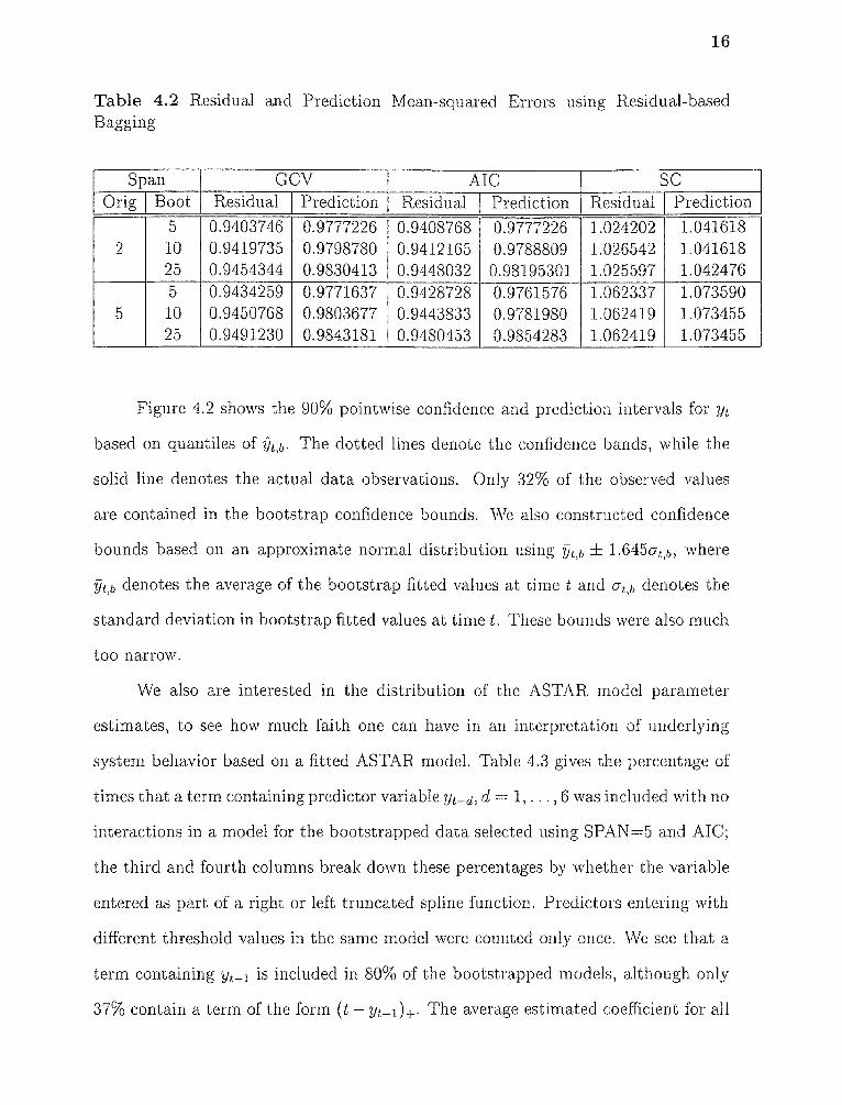
Table 4.2 Residual and Prediction Mean-squared Errors using Residual-basedBagging

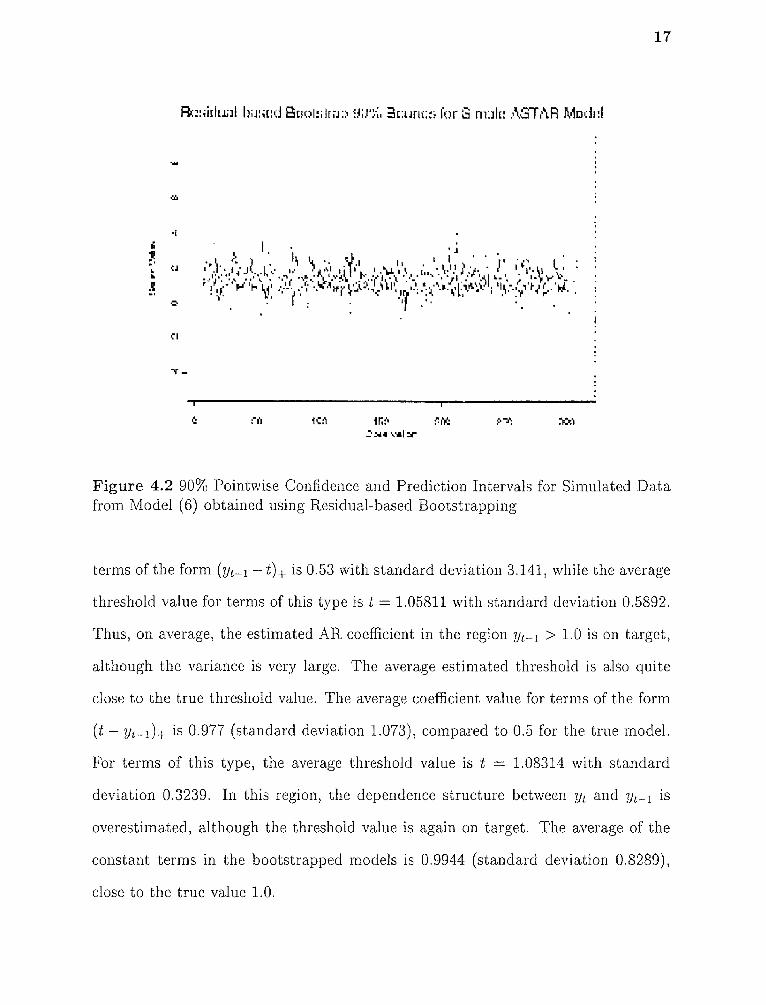
Figure 4.2 shows the 90% pointwise confidence and prediction intervals for y t

based on quantiles of y t , b • The dotted lines denote the confidence bands, while the

solid line denotes the actual data observations. Only 32% of the observed values

are contained in the bootstrap confidence bounds. We also constructed confidence

bounds based on an approximate normal distribution using yt,b 1.645σt,b, where

yt,bdenotes the average of the bootstrap fitted values at timetandσt,bdenotes the

standard deviation in bootstrap fitted values at time t. These bounds were also much

too narrow.

We also are interested in the distribution of the ASTAR model parameter

estimates, to see how much faith one can have in an interpretation of underlying

system behavior based on a fitted ASTAR model. Table 4.3 gives the percentage of

times that a term containing predictor variable y t- d , d = 1, . . , 6 was included with no

interactions in a model for the bootstrapped data selected using SPAN=5 and AIC;

the third and fourth columns break down these percentages by whether the variable

entered as part of a right or left truncated spline function. Predictors entering with

different threshold values in the same model were counted only once. We see that a

term containing yt - 1 is included in 80% of the bootstrapped models, although only

37% contain a term of the form (t — The average estimated coefficient for all

1:unc.ti. for CI' r1:31c: ASTAR Mud

17

Figure 4.2 90% Pointwise Confidence and Prediction Intervals for Simulated Datafrom Model (6) obtained using Residual-based Bootstrapping

terms of the form (y t- 1—0+is 0.53 with standard deviation 3.141, while the average

threshold value for terms of this type is t = 1.05811 with standard deviation 0.5892.

Thus, on average, the estimated AR coefficient in the region yt - 1 > 1.0 is on target,

although the variance is very large. The average estimated threshold is also quite

close to the true threshold value. The average coefficient value for terms of the form

(t — yt - 1) + is 0.977 (standard deviation 1.073), compared to 0.5 for the true model.

For terms of this type, the average threshold value is t = 1.08314 with standard

deviation 0.3239. In this region, the dependence structure between y t and yt- 1 is

overestimated, although the threshold value is again on target. The average of the

constant terms in the bootstrapped models is 0.9944 (standard deviation 0.8289),

close to the true value 1.0.

18

Table 4.3 Bootstrap Probabilities of obtaining a First-level Interaction Termcontaining yt - d

Table 4.4 Residual and Prediction Mean-squared Errors using Bagging forRegression-based Bootstrapping

Table 4.4 gives MSE results using regression-based bootstrapping. We see that

the regression-based bootstrap method gives an improvement in residual MSE for

all selected spans and model selection criteria. The improvement is greatest, about

15%, when a moderate span and the GCV or AIC selection criteria are used. The

forecast MSE improves only for models selected using the SC criterion. As discussed

in chapter 2, the SC criterion penalizes more heavily for additional parameters in the

model; the superior forecast performance for SC selected models indicates that the

other MSC may be over-fitting the data, thus giving good in-sample performance,

but worse out-of-sample performance. The improvement in forecast MSE with the

SC using bagging is only about 7%, however.

Figure 4.3 shows the 90% pointwise confidence and prediction intervals for y t

obtained using regression-based bootstrapping with MSC=AIC and Span=5. About

62% of the observed values are contained in the confidence bounds. Thus, although

19

the regression-based bounds give better coverage than the residual-based bounds,

both bootstrap methods underestimate the true variability in the underlying process

nnt for mr,I ASTAR Model

Figure 4.3 90% Pointwise Regression-based Bootstrap Confidence and PredictionIntervals for Series Generated from Model (6)

Table 4.5 gives the bootstrap probabilities for first-level interaction terms

containing yt - p using regression-based bootstrapping. Compared to the residual-

based bootstrap results, there is a higher probability that unnecessary predictor

variables (yt-p,p > 1) will be included in the model. The average estimated

coefficient for all terms of the form (y t-1 — t) 4_ is 0.528 with standard deviation

10.806, while the average threshold value is t = 1.319 (standard deviation 0.9373).

The average coefficient value for terms of the form (t — y t-1) + is 2.133 with standard

deviation 2.944. For terms of this type, the average threshold value is t = 0.8889

(standard deviation 0.3576). The average of the constant terms in the models is

0.9512 (standard deviation 3.14). Again, although the average AR(1) coefficient

for the region y t-1 is close to the true value of 0.5, the variability in estimated

coefficients is even larger than for the residual-based bootstrapping.

20

Table 4.5 Bootstrap Probabilities of obtaining a First-level Interaction Termcontaining yt - p using Regression-based Bootstrapping

4.2 An ASTAR Model with Interactions

To examine the stability of TSMARS for data generated from more complicated

ASTAR models, such as those containing interactions between predictor variables,

we simulated a series of length n = 312 from the following generating process.

y t = 0.0019 — 0.395(y t- 12 — 0.014) + (4.3)

—1.3822(0.018 — yt-2)+(yt-12 — 0.014) + + Et,

where e t are i.i.d. standard Normal random variables. The terms in the model are

the same as the first 2 terms of a fitted ASTAR model for weekly US $/Japanese

Yen exchange rates obtained by De Gooijer, Ray, and Krager (1998), in a study

of TSMARS models for forecasting exchange rates. Figure 4.4 shows the simulated

series.

As in the previous example, we used n o = 300 observations for model fitting

and used the remaining nv = 12 observations for forecast evaluation. We allowed up

to d = 24 possible predictors in the estimated model, with interactions up to level

MI = 3. The number of basis functions allowed in the forward steps of the algorithm

was MB = 40.

Using Span=5, MSC=SC, we obtained the following ASTAR model:

= —.064386 — 1.4547(0.189 — yt-2)+(yt-12 + 0.026)+ (4.4)

21

0 50 100 150 200 250 300

Figure 4.4 Simulated Data from ASTAR Model (9)

Table 4.6 Residual and Prediction Mean-squared Errors for Original Model

The fitted model picks up the nonlinear interaction between y t-2 and yt-12 with

approximately the correct spline and coefficient terms, but the threshold value for

yt-2 is much too large. The level-one interaction term is not estimated at all. Models

obtained using GCV or AIC were much more complex than that of (4.4), containing

several three-level interactions; a level-one y 1 - 1 2 right-truncated spline term and a

two-level interaction term exactly like that in (4.4) were included in the AIC and

GCV selected models, however.

Table 4.6 gives the mean-squared residual and prediction errors for models

estimated using the original data. Table 4.7 gives the results based on bootstrap

aggregation using residual-based bootstrapping. Table 4.8 gives results using

22

Table 4.7 Residual and Prediction Mean-squared Errors using Residual-basedBagging

Table 4.8 Residual and Prediction Mean-squared Errors using Bagging forRegression-based Bootstrapping

23

regression-based bootstrapping. All bootstrap results are based on 500 replications.

Residual-based bootstrapping gives reductions in residual MSE only for Span 25

models and reduces forecast MSE only for orignal Span 2 bootstrapped models

selected using GCV and the Span 2/5 model selected using SC. Regression-based

bootstrapping gives an improvement in residual MSE for all selected spans and

model selection criteria. The improvement is greatest, about 15%, when a moderate

span and the GCV or AIC selection criteria are used. The prediction MSE improves

only for the Span 5 and Span 25, SC selected models. The prediction MSEs for the

other SPAN, MSC combinations are very large or even infinite. A value of infinity

indicates that for certain bootstrap models, iterative forecasts "blow up", suggesting

instability of the bootstrapped model. The complexity of ASTAR processes makes it

very difficult to understand the stationarity and ergodicity properties of the models.

These issues may be investigated via simulation, as in De Gooijer and Brännas

(1995), and are an area for future research. As a way around the problem in

practice, a check can be used in the bootstrap algorithm to discard unstable models

having extremely large predicted values.

CHAPTER 5

AN APPLICATION

The series of yearly Wolf sunspot numbers, a measure of the average monthly sunspot

activity on the surface of the sun, has been the focus of much analysis in time

series because of its interesting nonsymmetric cyclic behavior. Tong (1983; 1990)

attempted to model the series using a TAR model, while Rao and Gabr (1984)

used a bilinear model. Figure 5.3 shows a time series plot of the sunspot data over

the period 1700-1920. We see that the data behaves in a periodic fashion, with

extremely sharp peaks and troughs, although the cycles vary from 10 to 12 years.

A greater number of sunspots is concentrated in each descent period relative to the

number in the corresponding ascent period. Lewis and Stevens (1991) applied the

TSMARS methodology to the sunspot data, allowing up to d = 20 lagged values of

the series as predictors. They obtained various models by trying different algorithm

parameter values and report detailed analysis for a model obtained using MI=3,

MB=15, and SPAN=18. In their analysis, model selection was done using GCV.

Their fitted model contained nonzero single-factor terms at lags 1, 5, and 9, with

interactions between sunspot values lagged by 1 and 2 months, 1 and 3 months, 1

and 4 months, and 1, 2, and 5 months. Because of the lack of inference methods for

ASTAR models, however, it is unclear whether each of the estimated terms in their

model is statistically significant. Lewis and Stevens also obtained predictions for the

sunspot data for the years 1921-1955. Although they were able to show that their

fitted ASTAR models improved significantly upon alternative linear and nonlinear

models using out-of-sample validation, they did not provide prediction intervals.

In this chapter, we apply the bootstrap methods of chapter 3 to the sunspot

data. We want to see if bootstrapping can be used to obtain more stable fits and

forecasts, as well as to obtain reliable bootstrap confidence and prediction intervals.

24

Regression-based Bootstrap 90% Bounds for Yearly Sunspot Data

25

Year

Figure 5.1 90% Confidence and Prediction Bounds for Sunspot Data usingRegression-based Bootstrapping

We use the same number of predictors, forward basis functions, and maximum inter-

actions as Lewis and Stevens (1991), varying the span parameter and the model

selection criterion to assess their effect on the original and bootstrapped model

results. We use the fitted models to iteratively predict the sunspot numbers five years

into the future. Predictions from many of the bootstrapped models were unstable at

lead times longer than five years.

Table 5.1 gives residual and prediction MSEs for the original sunspot data using

different spans and model selection criteria. The AIC model selection criterion with

Span=9 gives the smallest in-sample residual mean-squared error, while the Span 9,

SC model provides the best out-of-sample forecast performance. Analogous results

are true for models fitted using Span=18.

Table 5.2 gives results based on Bagging models for residual-based bootstrapped

data. Bagging does not reduce in-sample MSEs except for models selected using SC,

but substantially reduces out-of-sample forecast MSEs about 15% on average for all

analyzed spans and selection criteria.

26

True and Filed Values -for Yearly Sunspot Numbers

E

Figure 5.2 Fitted Values from Original and Bagged Models for Sunspot Dataselected using Span 9 and MSC=SC

Table 5.1 Residual and Prediction Mean-squared Errors for ASTAR Models ofSunspot Data

Table 5.3 give results based on Bagging models for regression-based bootstrapped

data. We see that regression-based bootstrapping using Span=9 gives a reduction

in residual MSE of about 26% when a model is selected using GCV or AIC. The

reduction in residual MSE is almost 40% when the SC is used for model selection,

however the prediction MSE is only reduced by about 5% when MSC=SC and

Span=9. Reductions in prediction MSE for the GCV and AIC model selection

criteria are much larger, between 21% and 29%. Similar results hold when Span

18 is used, although the reduction in prediction MSE using SC is larger than that

obtained using Span=9. Using the AIC or GCV criteria with a smaller SPAN

27

Figure 5.3 Yearly Wolf Sunspot Numbers, 1700-1920

seems to reduce in-sample prediction error, but increases out-of-sample forecast

performance. The algorithm is most likely over-fitting the data, resulting in poor out-

of-sample forecasts. Overall, residual-based bootstrapping gives greater decreases in

residual and prediction MSEs than regression-based bootstrapping for the sunspot

data using the SC for model selection.

Figure 5.1 shows 90% confidence and prediction intervals for the sunspot

data obtained using Span=9, MSC=SC and regression-based bootstrapping. The

confidence bounds contain only 76% of the observed data values; the prediction

bounds do not completely capture the bottom of sunspot cycle. Figure 5.2 shows

observed and fitted sunspot values from the original model using Span 9 and

MSC=SC, along with the fitted values obtained using Bagging of regression-based

bootstrap results. The solid line in the plot shows the standard deviation in bootstrap

fitted values. The vertical line at t = 201 marks the beginning of predicted values.

28

Table 5.2 Residual and Prediction Mean-squared Errors for Sunspot Data usingResidual-based Bootstrapping

Table 5.3 Residual and Prediction Mean-squared Errors for Regression-basedBootstrapped TSMARS Models of Sunspot Data

Table 5.4 Bootstrap Probabilities of obtaining a First-level Interaction Termcontaining yt - p using Regression-based Bootstrapping

29

We see that the standard deviations are higher when the sunspots values are near the

top of their cycle. Additionally, the fitted values from the original model sometimes

take negative values, while the bootstrap fitted values are all positive.

Table 5.4 gives the percentage of regression-based bootstrapped models

containing a yt—d level-one interaction term and the percentage of times the term

was of the form of a right (1.4) or left (p__) truncated spline. Only lagged terms

appearing in at least 5% of the bootstrapped models are included in the table. We

see that a term involving y t-1 appears in almost every model, primarily in the form

of a right-truncated spline function. Lag 2 and Lag 9 terms also appear in a large

percentage of the bootstrapped models. The original model of Lewis and Stevens

(1991) contained Lag 1, Lag 5, and Lag 9 first-order interaction terms. The small

percentage of bootstrapped models containing a Lag 5 terms casts doubt on the

significance of this term in the original model.

CHAPTER 6

DISCUSSION

Bootstrapping provides a simple method for obtaining confidence bounds and

prediction intervals for data modeled using TSMARS, however for the examples

presented here, coverage of the bootstrap intervals was consistently too small.

In general, residual-based bootstrapping seems to provide greater reductions in

residual and prediction MSEs, while confidence intervals based on regression-based

bootstrapping provide coverage closer to nominal. We prefer the regression-based

method, as it is a nonparametric procedure. Although the bootstrap methods

discussed here can provide estimated parameter distributions for lagged and

thresholded predictor variables, it can become extremely complicated to categorize

these estimates by level of interaction, predictor lag, and term type (right or left

truncation), as the number of possible categories has the potential to be quite

large for even moderate values of d when MI > 2. The importance of different

predictor variables can, however, be assessed by looking at the percentage of times

a particular lagged variable appears in the bootstrapped models, regardless of the

term type. This type of result is similar to that obtained using the Bayesian MARS

methodology of Dennison and Mallik (1997), although their implementation of the

MARS procedure is more restrictive in that many algorithm parameters, such as MI

and Span ,are fixed.

Future world will examine other bootstrap methods for ASTAR models, such

as the wild bootstrap. Consistency results for bootstrap procedures in the TSMARS

framework present many challenging theoretical problems.

30

REFERENCES

Berkowitz, J. and Kilian, L. (1996). "Recent developments in bootstrapping timeseries," Technical Report # 1996-45, Finance and Economics Discussion Series,Division of Research and Statistics and Monetary Affairs, Federal Reserve Board,Washington, D.C.

Breiman, L. (1996). "Bagging predictors", Machine Learning, 24, 123-140.

Breiman, L., Friedman, J. H., Olshen, R. and Stone, C. J. (1984). Classification andregression trees, Wadsworth, Belmont, California.

Chatterjee, S. (1986). "Bootstrapping ARMA models: some simulations," IEEETransactions Systems, Man and Cybernetics, SMC- 16, 294-299.

De Gooijer, J. G. and Brännas, K. (1995). Invertibility of non-linear time seriesmodels," Commun. Statist. Theory Math., 241, 2701-2714.

De Gooijer, J., Ray, B., and Krager, H. (1998). "Forecasting exchange rates usingTSMARS", International Journal of Money and Finance, forthcoming.

Denison, D. G. T. and Mallick, B. K. (1997). "Bayesian MARS", preprint, ImperialCollege, London.

Efron, B. and Tibshirani, R. (1993). An introduction to the bootstrap, New York:Chapman and Hall.

Franke, J., Kreiss, J. P., and Mammen, E. (1997). 'Bootstrap of kernel smoothingin nonlinear time series", preprint, University of Heidelberg, Heidelberg.

Friedman, J. H. (1991). "Multivariate adaptive regression splines", Annals ofStatistics 19, 1 -142.

Friedman, J. H. (1993), "Fast MARS", Technical Report 100, Department ofStatistics, Stanford University, California.

Kunsch, H. R. (1989). "The jackknife and the bootstrap for general stationaryobservations", The Annals of Statistics, 17, 1217-1241.

Lall, U., Sangoyomi, T. and Abarbanel, H. (1996). " Nonlinear dynamics of the GreatSalt Lake: Nonparametric short-term forecasting," Water Resources Research, 32,

975-1004

Lall, U., Sangoyomi, T. and Abarbanel, H. (1996). "A nearest neighbor bootstrapfor resampling hydrologic time series", Water Resources Research , 32, 679-694.

31

32

Lewis, P. A. W. and Stevens, J. G. (1991). 'Nonlinear modeling of time seriesusing Multivariate Adaptive Regression Splines (MARS)", Journal of the AmericanStatistical Association, 87, 864-877.

Lewis, P. A. W. and Ray, B. K. (1993). "Nonlinear modelling of multivariate andcategorical time series using Multivariate Adaptive Regession Splines", DimensionEstimation and Models, ed. H,Tong, Singapore: World Scientific, 136-169.

Lewis, P. A. W. and Ray, B. K. (1997). " Modeling long-range dependence, nonlin-earity, and periodic phenomena in sea surface temperatures using TSMARS" , Journalof the American Statistical Association , 92, 881-893.

Liu, R. and Singh, K. (1992). "Moving blocks jackknife and bootstrap capture weakdependence," in Exploring the Limits of Bootstrap, R. LePage and L. Billard, eds.New York: John Wiley & Sons.

Masaratto, G. (1990). "Bootstrapping prediction intervals for autoregressions,"International Journal of Forecasting, 6, 229-239.

Morgan, J. N. and Sonquist, J. A. (1963). "Problems in the analysis of survey dataand a proposal", Journal of the American Statistical Association , 58, 415-434.

Neumann, M. and Kreiss, J. P. (1997). "Bootstrap condfidence bands for the autore-gression function," preprint, University of Heidelberg, Heidelberg.

Rao, S. T., and Gabr, M. M. (1984). An introduction to bispectral analysis andbilinear time series models, Berlin: Springer-Verlag.

Schwarz, G. (1978). "Estimating the dimension of a model," Annals of Statistics, 6,461-464.

Stevens, J. G.(1991). "An investigation of multivariate adaptive regression splinesfor modeling and analysis of univriate and semi-multivariate sime series systems",Ph.D. thesis, Naval Postgraduate School, Monterey, California.

Stine, R. A. (1987). "Estimating properties of autoregressive forecasts," Journal ofthe American Statistical Association, 82, 1072-1078.

Tong, H. (1983). Threshold models in nonlinear time series analysis, New York:Springer-Verlag.

Tong, H.(1990). Nonlinear time series, New York: Oxford University Press.