Bootstrap in Finance

Esther Ruiz and Maria Rosa Nieto(A. Rodríguez, J. Romo and L. Pascual)

Department of Statistics

UNIVERSIDAD CARLOS III DE MADRID

Workshop Modelling and Numerical Techniques in Quantitative Finance

A Coruña 15 de octubre de 2009

Motivation Bootstrapping to obtain prediction densities of

future returns and volatilities GARCH Stochastic volatility

Bootstrapping to measure risk: VaR and Expected Shortfall

Conclusions

1. Motivation

High frequency time series of returns are characterized by volatility clustering: Excess kurtosis Significant autocorrelations of absolute

returns (not independent)

-4

-3

-2

-1

0

1

2

3

4

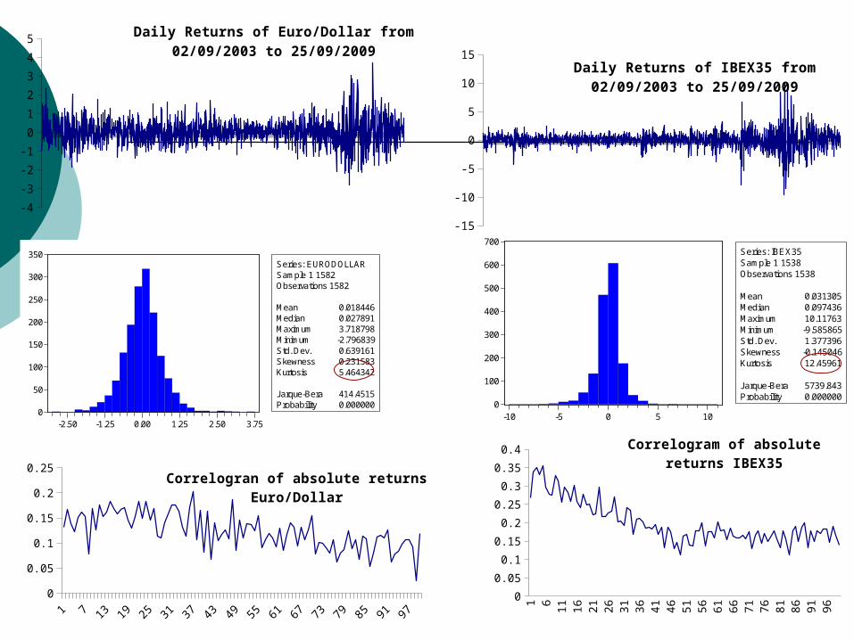
5Daily Returns of Euro/Dollar from 02/09/2003

to 25/09/2009

0

50

100

150

200

250

300

350

-2.50 -1.25 0.00 1.25 2.50 3.75

Series: EURODOLLARSample 1 1582Observations 1582

Mean 0.018446Median 0.027891Maximum 3.718798Minimum -2.796839Std. Dev. 0.639161Skewness 0.231583Kurtosis 5.464342

Jarque-Bera 414.4515Probability 0.000000

0

0.05

0.1

0.15

0.2

0.25Correlogran of absolute returns Euro/Dollar

-15

-10

-5

0

5

10

15Daily Returns of IBEX35 from 02/09/2003 to

25/09/2009

0

100

200

300

400

500

600

700

-10 -5 0 5 10

Series: IBEX35Sample 1 1538Observations 1538

Mean 0.031305Median 0.097436Maximum 10.11763Minimum -9.585865Std. Dev. 1.377396Skewness -0.145046Kurtosis 12.45961

Jarque-Bera 5739.843Probability 0.000000

1 6 11 16 21 26 31 36 41 46 51 56 61 66 71 76 81 86 91 96

0

0.05

0.1

0.15

0.2

0.25

0.3

0.35

0.4Correlogram of absolute returns IBEX35

Financial models based on inference on the dynamic behaviour of returns and/or predictions of moments associated with the density of future returns which assume independent and/or Gaussian observations are inadequate.

Bootstrap methos are attractive in this context because they do not assume any particular distribution.

However, bootstrap procedures cannot be based on resampling directly from observed returns as they are not indepedent.

Assume a parametric specification of the dependence and bootstrap from the corresponding residuals.

Generalize the bootstrap procedures to cope with dependent observations

Li and maddala (1996) and Berkowitz and Kilian (2000) show that the parametric approach could be preferable in many applications.

Consequently, we focus on two of the most popular and simpler models to represent the dynamic properties of financial returns:

GARCH(1,1)

ARSV(1)

ttty

21

21

2 ttt y

ttt 2

12 loglog

-4

-3

-2

-1

0

1

2

3

4GARCH(1,1)-N: 0.5, 0.15, 0.8

0

40

80

120

160

200

-2.50 -1.25 0.00 1.25 2.50

Series: GNSample 1 1500Observations 1500

Mean -0.011948Median 0.024450Maximum 3.387700Minimum -3.136800Std. Dev. 0.899944Skewness 0.014030Kurtosis 3.501793

Jarque-Bera 15.78648Probability 0.000373

1 5 9 13 17 21 25 29 33 37 41 45 49 53 57 61 65 69 73 77 81 85 89 93 97

-0.1

-0.05

0

0.05

0.1

0.15 Correlogram of absolute returns GARCH(1,1)-N

-15

-10

-5

0

5

10 SV: 0.05, 0.95, 0.05

0

40

80

120

160

200

240

-10.0 -7.5 -5.0 -2.5 0.0 2.5 5.0 7.5

Series: SVSample 1 1500Observations 1500

Mean -0.060025Median -0.007813Maximum 8.578551Minimum -9.568826Std. Dev. 1.830458Skewness -0.131483Kurtosis 4.666630

Jarque-Bera 177.9254Probability 0.000000

1 6 11 16 21 26 31 36 41 46 51 56 61 66 71 76 81 86 91 96

-0.04

-0.02

0

0.02

0.04

0.06

0.08

0.1

0.12

0.14Correlogram of absolute returns SV

There are two main related areas of application of bootstrap methods Inference: Obtaining the sample distribution of

a particular estimator or a statistic for testing, for example, the autoregressive dynamics in the conditional mean and variance, unit roots in the mean, fractional integration in volatility, inference for trading rules: Ruiz and Pascual (2002, JES)

Prediction: Prediction of future densities of returns and volatilities: VaR and ES

Bootstrap methods allow to obtain prediction densities (intervals) of future returns without distributional assumptions on the prediction error distribution and incorporating the parameter uncertainty Thombs and Schucany (1990, JASA):

backward representation Cao et al. (1997, CSSC): conditional on

estimated parameters Pascual et al. (2004, JTSA): incorporate

parameter undertainty without backward representation

Example AR(1)The Minimum MSE predictor of yT+k based on the

information available at time T is given by its conditional mean

where

In practice, the parameters are substituted by consistent estimates. Therefore, the predictions are given by

1~~

kTkT yy

TT yy ~

Predictions are made conditional on the available data

1ˆˆˆˆ kTkT yy

Thombs and Schucany (1990)

where are bootstrap replicates of the standardized residuals and are obtained from bootstrap replicates of the series based on the backward representation

where

**1

*** ˆˆ kTkTkT ayy

*kTa

** ,

**1

* ˆˆ TTt ayy

TT yy *

Should we fix yT when bootstrapping the parameters???

NO

Pascual et al. (2004, JTSA) propose a bootstrap procedure to obtain prediction intervals in ARIMA models that do not requiere the backward representation. Therefore, this procedure is simpler and more general, as it can cope with models for which the backward representation does not exist as, for example, GARCH.

2. Bootstrap forecast of future returns and volatilities

We consider the prediction of future returns and volatilities generated by GARCH and ARSV(1) models

2.1 GARCH

2.2 ARSV

Both models provide prediction intervals which are narrow in quite times and wide in volatile periods.

21

21

2 ttt y

ttt 2

12 loglog

2.1 GARCH (1,1): Pascual et al. (2005, CSDA)

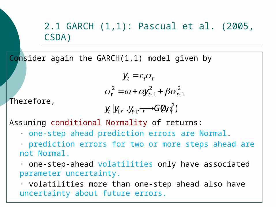
Consider again the GARCH(1,1) model given by

Therefore,

Assuming conditional Normality of returns:· one-step ahead prediction errors are Normal.· prediction errors for two or more steps ahead are not Normal.· one-step-ahead volatilities only have associated parameter uncertainty.· volatilities more than one-step ahead also have uncertainty about future errors.

ttty 2

12

12

ttt y

),0(,...,| 211 ttt Gyyy

Bootstrap procedure

Estimate parameters and obtain standardized residuals Obtain bootstrap replicates of the series

and estimate the parameters. Bootstrap forecasts of future returns and volatilities

***

2*1

2*1

2* ˆˆˆ

ttt

ttt

y

y

2

0**

*2

1**

**

*2*

*

***

2*1

*2*1

**2*

ˆˆ1

ˆˆˆˆˆ1

ˆ

ˆˆˆ

T

jjT

jT

TT

kTkTkT

kTkTkT

y

yy

y

y

Using the bootstrap estimates of the parameters with the original observations (conditional)

-8 -6 -4 -2 0 2 40

0.1

0.2

0.3

0.4

0.5

0.6

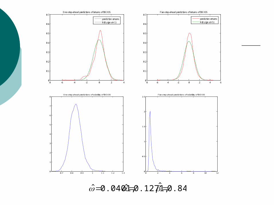
0.7One-step-ahead predictions of returns of IBEX35

-8 -6 -4 -2 0 2 4 60

0.1

0.2

0.3

0.4

0.5

0.6

0.7Five-step-ahead predictions of returns of IBEX35

prediction returns

N(0,sigmat+1)

prediction returns

N(0,sigmat+5)

0.7 0.8 0.9 1 1.1 1.2 1.30

1

2

3

4

5

6

7

8One-step-ahead predictions of volatility of IBEX35

0 2 4 6 8 10 120

0.5

1

1.5

2

2.5Five-step-ahead predictions of volatility of IBEX35

0.8481ˆ 0.1271,ˆ 0.0401,ˆ

-3 -2 -1 0 1 2 30

0.1

0.2

0.3

0.4

0.5

0.6

0.7

0.8

0.9

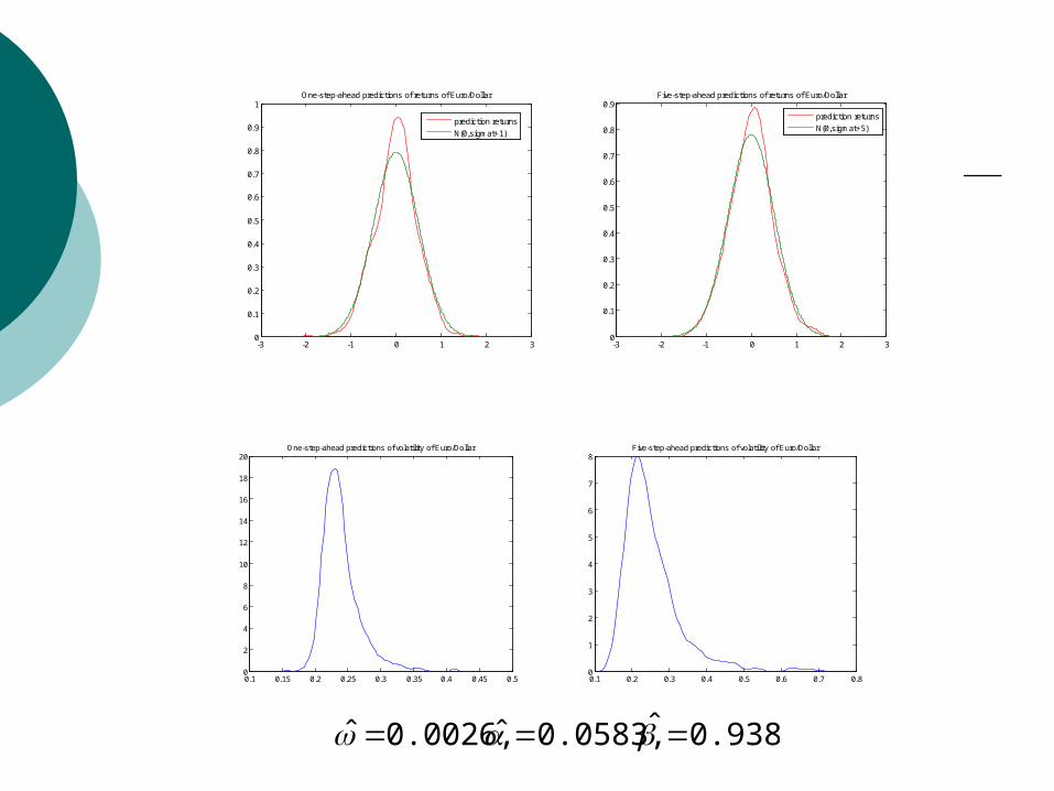
1One-step-ahead predictions of returns of Euro/Dollar

-3 -2 -1 0 1 2 30

0.1

0.2

0.3

0.4

0.5

0.6

0.7

0.8

0.9Five-step-ahead predictions of returns of Euro/Dollar

prediction returns

N(0,sigmat+1)

prediction returns

N(0,sigmat+5)

0.1 0.15 0.2 0.25 0.3 0.35 0.4 0.45 0.50

2

4

6

8

10

12

14

16

18

20One-step-ahead predictions of volatility of Euro/Dollar

0.1 0.2 0.3 0.4 0.5 0.6 0.7 0.80

1

2

3

4

5

6

7

8Five-step-ahead predictions of volatility of Euro/Dollar

0.9387ˆ 0.0583,ˆ 0.0026, ˆ

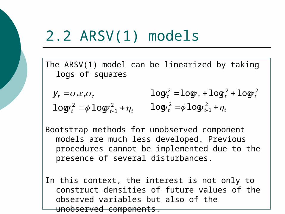
2.2 ARSV(1) models

The ARSV(1) model can be linearized by taking logs of squares

Bootstrap methods for unobserved component models are much less developed. Previous procedures cannot be implemented due to the presence of several disturbances.

In this context, the interest is not only to construct densities of future values of the observed variables but also of the unobserved components.

ttt

ttty

2

12

22*

2

loglog

loglogloglog

ttt

ttty

2

12

*

loglog

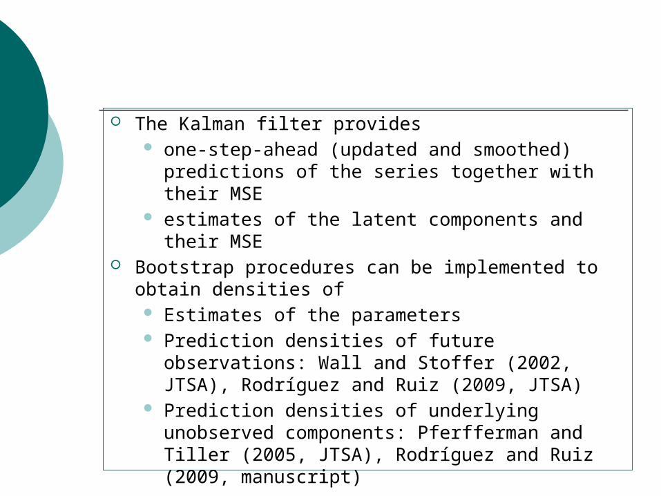
The Kalman filter provides one-step-ahead (updated and smoothed)

predictions of the series together with their MSE estimates of the latent components and their

MSE Bootstrap procedures can be implemented to obtain

densities of Estimates of the parameters Prediction densities of future observations: Wall

and Stoffer (2002, JTSA), Rodríguez and Ruiz (2009, JTSA)

Prediction densities of underlying unobserved components: Pferfferman and Tiller (2005, JTSA), Rodríguez and Ruiz (2009, manuscript)

Rodríguez and Ruiz (2009, JTSA) propose a bootstrap procedure to obtain prediction intervals of future observations in unobserved component models that incorporate the parameter uncertainty without using the backward representation.

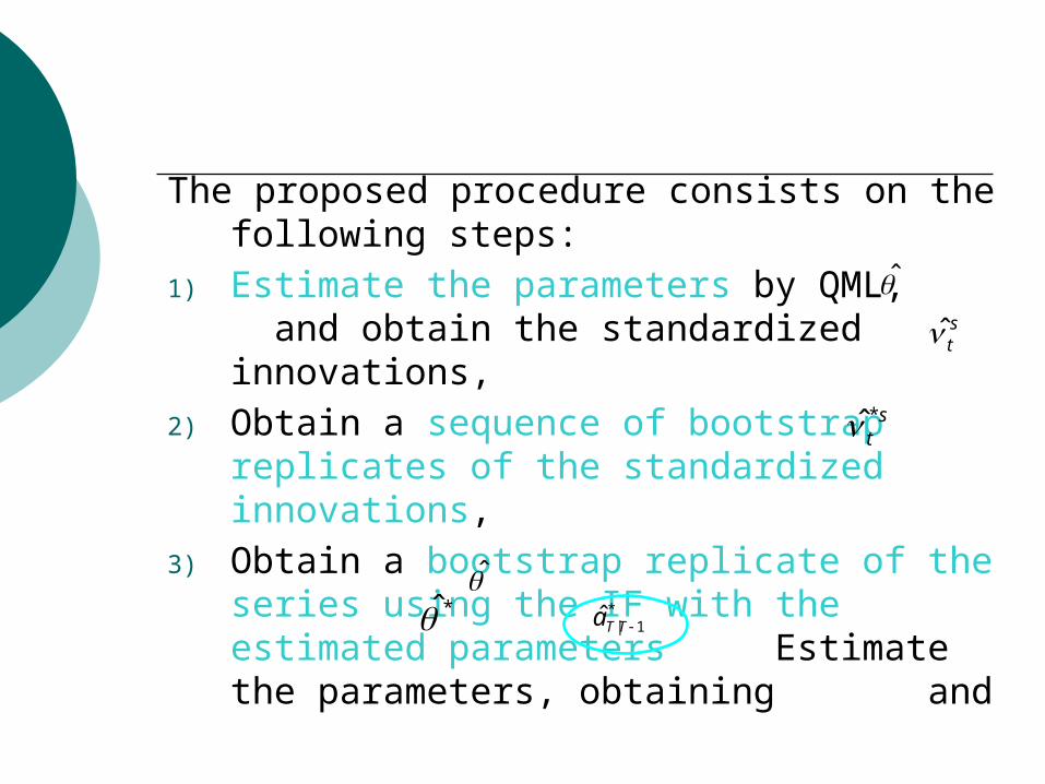
The proposed procedure consists on the following steps:

1) Estimate the parameters by QML, and obtain the standardized innovations,

2) Obtain a sequence of bootstrap replicates of the standardized innovations,

3) Obtain a bootstrap replicate of the series using the IF with the estimated parameters Estimate the parameters, obtaining and

st

st*

* *

1|ˆ TTa

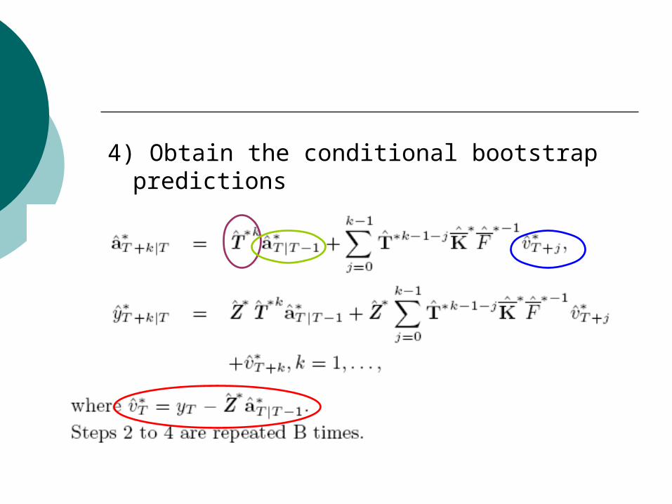
4) Obtain the conditional bootstrap predictions

However, as we mentioned before, when modelling volatility, the objective is not only to predict the density of future returns but also to predict future volatilities. Therefore, we need to obtain prediction intervals for the unobserved components.

At the moment, Rodríguez and Ruiz (2009, manuscript) propose a procedure to obtain the MSE of the unobserved components.

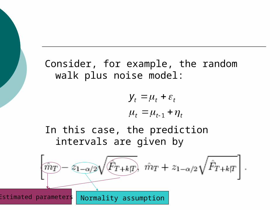
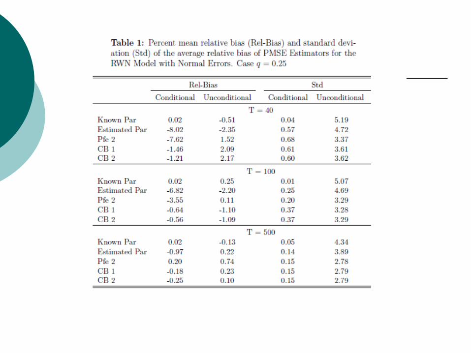
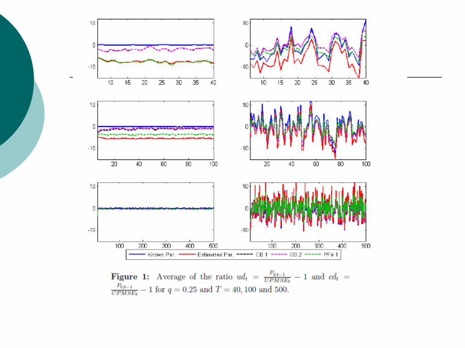
Consider, for example, the random walk plus noise model:

In this case, the prediction intervals are given by

ttt

ttty

1

Normality assumptionEstimated parameters

Random walk with q=0.5Estimates of the level and 95% confidence intervals: In red with

estimated parameters and in black with known parameters.

Our procedure is based on the following decomposition of the MSE proposed by Hamilton (1986)

He proposes to generate replicates of the parameters from the asymptotic distribution and then to estimate the MSE by

The filter is run with original observations

We propose a non-parametric bootstrap in which the bootstrap replicates of the series are obtained from the innovation form after resampling from the innovations.

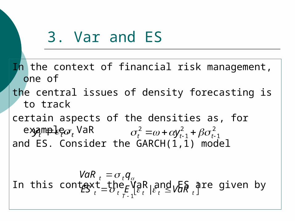
3. Var and ES

In the context of financial risk management, one ofthe central issues of density forecasting is to trackcertain aspects of the densities as, for example, VaRand ES. Consider the GARCH(1,1) model

In this context the VaR and ES are given by

21

21

2 ttt y ttty

tttTtt

tt

VaREES

qVaR

|1

In practice, assuming that the model is known, both the parameters and the distribution of the errors are unknown. Therefore, we obtain the estimates

Bootstrap procedures have been proposed to obtain point estimates of the VaR by computing the corresponding quantile of the bootstrap distribution of returns (Ruiz and Pascual, 2004, JES)

tttttt

tt

VaREES

qRaV

|ˆ

ˆˆˆ

1

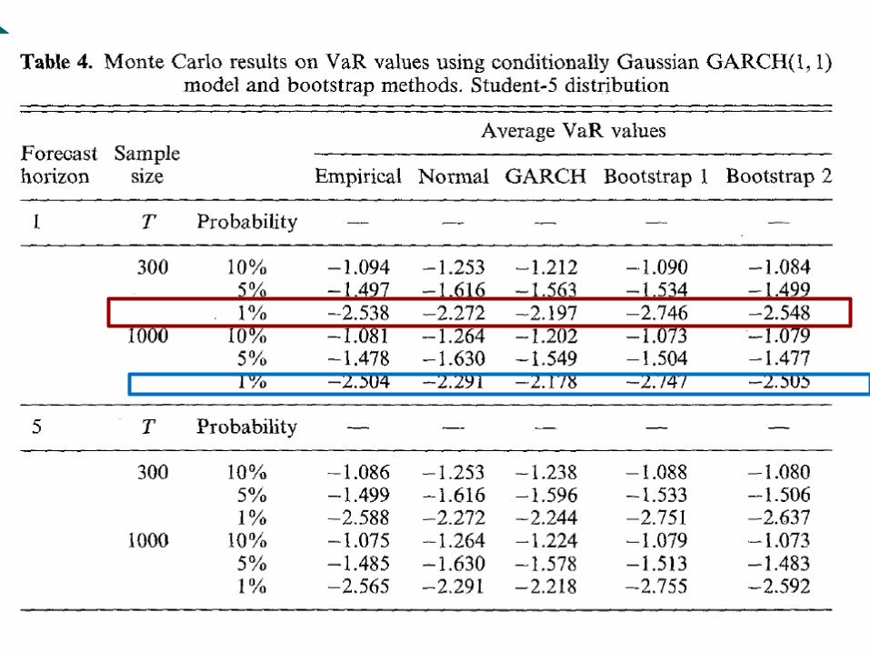
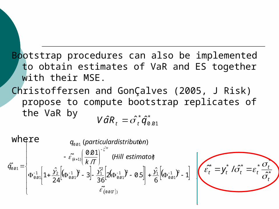
Bootstrap procedures can also be implemented to obtain estimates of VaR and ES together with their MSE.

Christoffersen and GonÇalves (2005, J Risk) propose to compute bootstrap replicates of the VaR by

where*

01.0* ˆˆˆ qRaV tt

*)01.0(

2101.0

12101.0

2121

01.021

01.0

ˆ

*)1(

01.0

*01.0

ˆ

16

ˆ5.02

36

ˆ3

24

ˆ1

)(/

01.0ˆ

)(

ˆ

T

k estimatorHillTk

ondistributiparticularq

q

H

*

*****

ˆˆ/ˆ

t

ttttt y

Instead of using the residuals obtained in each of the bootstrap replicates of the original series, Nieto and Ruiz (2009, manuscript) propose to estimate q0.01 by a second bootstrap step.

For each bootstrap replicate of the series of returns, we obtain n random draws from the empirical distribution of the original standardized residuals, Then, the constant q0.01 can be estimated by any of the three alternative estimators described before.

In this way, we avoid the estimation error involved in the residuals

t

*

***

ˆˆ

t

ttt

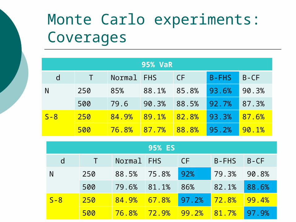
Monte Carlo experiments: Coverages

95% VaR

d T Normal FHS CF B-FHS B-CF

N 250 85% 88.1% 85.8% 93.6% 90.3%

500 79.6 90.3% 88.5% 92.7% 87.3%

S-8 250 84.9% 89.1% 82.8% 93.3% 87.6%

500 76.8% 87.7% 88.8% 95.2% 90.1%

95% ES

d T Normal FHS CF B-FHS B-CF

N 250 88.5% 75.8% 92% 79.3% 90.8%

500 79.6% 81.1% 86% 82.1% 88.6%

S-8 250 84.9% 67.8% 97.2% 72.8% 99.4%

500 76.8% 72.9% 99.2% 81.7% 97.9%

-4.5 -4 -3.5 -3 -2.5 -2 -1.50

0.5

1

1.5

2

2.5

3

3.5

4

4.5

5

-5 -4.5 -4 -3.5 -3 -2.5 -2 -1.5 -10

0.5

1

1.5

2

2.5

3

3.5

4

4.5

VaRBootstrap

VaRCGN

VaRCGHVaRCGFHS

VaRCGGCCF

ESBootstrap

ESCGGN

ESCGGHESCGGFHS

ESCGGGCCF

Prediction bootstrap densities of VaR and ES for IBEX35

-2.2 -2 -1.8 -1.6 -1.4 -1.2 -1 -0.80

0.5

1

1.5

2

2.5

3

3.5

4

4.5

5

-3 -2.8 -2.6 -2.4 -2.2 -2 -1.8 -1.6 -1.4 -1.2 -10

0.5

1

1.5

2

2.5

3

3.5

4

VaRBootstrap

VaRCGN

VaRCGHVaRCGFHS

VaRCGGCCF

ESBootstrap

ESCGN

ESCGHESCGFHS

ESCGGCCF

Prediction bootstrap densities of VaR and ES for Euro/Dollar

Conclusions and further research

Few analytical results on the statistical properties of bootstrap procedures when applied to heterocedastic time series

Further improvements in: bootstrap estimation of quantiles and

expectations to compute the VaR and ES construction of prediction intervals for unobserved

components (stochastic volatility) Multivariate extensions: Engsted and

Tanggaard (2001, JEF)