Neural Networks 22 (2009) 748–756

Contents lists available at ScienceDirect

Neural Networks

journal homepage: www.elsevier.com/locate/neunet

2009 Special Issue

Boosting feature selection for Neural Network based regression

Kevin Bailly ∗, Maurice Milgram 1Institut des Systèmes Intelligents et de Robotique, Université Pierre et Marie Curie-Paris 6, CNRS, UMR 7222, 4 place Jussieu, 75005 Paris, France

a r t i c l e i n f o

Article history:Received 5 May 2009Received in revised form 11 June 2009Accepted 25 June 2009

Keywords:Input feature selectionBoostingRegressionFuzzy functional criterion

a b s t r a c t

The head pose estimation problem is well known to be a challenging task in computer vision and is auseful tool for several applications involving human–computer interaction. This problem can be stated asa regression one where the input is an image and the output is pan and tilt angles. Finding the optimalregression is a hard problem because of the high dimensionality of the input (number of image pixels)and the large variety of morphologies and illumination. We propose a newmethod combining a boostingstrategy for feature selection and a neural network for the regression. Potential features are a very largeset of Haar-like wavelets which are well known to be adapted to face image processing. To achieve thefeature selection, a new Fuzzy Functional Criterion (FFC) is introduced which is able to evaluate the linkbetween a feature and the output without any estimation of the joint probability density function as inthe Mutual Information. The boosting strategy uses this criterion at each step: features are evaluated bythe FFC using weights on examples computed from the error produced by the neural network trained atthe previous step. Tests are carried out on the commonly used Pointing 04 database and compared withthree state-of-the-art methods. We also evaluate the accuracy of the estimation on FacePix, a databasewith a high angular resolution. Our method is compared positively to a Convolutional Neural Network,which is well known to incorporate feature extraction in its first layers.

© 2009 Elsevier Ltd. All rights reserved.

1. Introduction

In a large number of regression problems, it is not easy to findrelevant features from a huge set of potential input variables. Inimage based regression for instance, the number of pixels, whichcorresponds to the input dimension, is very large. Moreover, pixellevel is not necessarily suitable for a particular problem and ahuge set of potential features can be extracted from an image tocomplete or to supply the necessary information. Just few of themare relevant, while most of them are redundant. In this paper, wepresent a framework to learn simultaneously relevant features andthe corresponding regressor.A large number of solutions have been proposed in the feature

selection literature. They can be divided into filter, wrapper andembedded approaches (Guyon & Elisseeff, 2003). In the filter basedmethod, features are first selected using a specific measure ofrelevance such asmutual information or Pearson’s correlation. Thesecond stage consists of estimating parameters of the regressionmodel on the selected subset. This approach is computationally

∗ Corresponding author. Tel.: +33(0)144276309.E-mail addresses: kbailly@gmail.com, kevin.bailly@isir.fr (K. Bailly),

maurice.milgram@upmc.fr (M. Milgram).1 Tel.: +33(0)144275197.

0893-6080/$ – see front matter© 2009 Elsevier Ltd. All rights reserved.doi:10.1016/j.neunet.2009.06.039

efficient, but presents amajor drawback (Kohavi & John, 1997): theregression model is not taken into account. Thus, a suboptimal setof relevant features tends to be selected rather than the completeset of useful features.Wrapper approaches use the prediction performance of the

model to quantify the relevance of a feature subset. In thiscategory, greedy forward selection algorithms are frequently used:they progressively integrate new variables which optimize theregression score. This strategy is really time consuming andintractable when the regression learning algorithm is too complex.Embedded approaches incorporate the feature selection di-

rectly into the learning algorithm. In ridge regression such asLASSO (Tibshirani, 1996) or Input Decay (Chapados & Bengio,2001), a regularization term is introduced in the cost function. Theaim is to train the model so that inputs which contribute poorlyto the regression process are penalized. These methods are wellsuited when the number of potential features is quite restricted.In Section 2, we introduce BISAR (Boosted Input Selection

Algorithm for Regression) which combines a filter and a wrapperapproach.BISAR uses a kind of boosting in the feature selection process.

In its simplest form, the boosting strategy aims to decrease theerror rate of a classifier/regressor by concentrating at each iterationon examples that are particularly difficult to classify/regress.This is usually done by iteratively adapting the training samplesweighting. At each iteration the weight of the training examples

K. Bailly, M. Milgram / Neural Networks 22 (2009) 748–756 749

depends on the performance of the classifier/regressor in theprevious iteration.AdaBoost (Freund & Schapire, 1995) is a popular algorithm

to iteratively build a classifier as a linear combination of theso-called weak classifiers. At each step, a new weak classifieris added optimizing the classification error rate with a newweighting on training samples. AdaBoost.RT, proposed by Shrestha(Shrestha & Solomatine, 2006) for regression problems uses theso-called absolute relative error threshold φ to project trainingexamples into two classes (poorly and well predicted examples)by comparing the absolute relative error with the thresholdφ. The problem is that it is not obvious to choose the rightvalue for the threshold φ. Therefore we have selected anotherboosting strategy, AdaBoost.R2 (Drucker, 1997), to compareseveral boosting strategies in BISAR. There are other methods likeRedpath and Lebart (2005) and Xu and Zhang (2006) that alsocombine these two approaches in a different way. The algorithmdescribed in Redpath and Lebart (2005) is clearly dedicated tosolving classification and not regression problems and aims toreduce the number of features used by each weak classifier. In Xuand Zhang (2006), an approach which limits the correlations of theselected feature set for gene selection in microarray data analysisis presented. This approach seems to be specific to this kind ofproblem and the boosting strategy is completely different fromBISAR.The two main contributions of this paper are:

1. The Fuzzy Functional Criterion (FFC): a new filter used to selectrelevant features (Section 2.1)

2. A new boosting strategy that selects incrementally newcomplementary inputs for the regressor (Section 2.3).

A large number of experiments (Section 3) with BISAR on aclassical pattern recognition problem is covered in this article(Section 4). Comparisons are drawn between BISAR and state-of-the-art methods (Section 5). Finally we present conclusions andprospects in Section 6.

2. Boosted Input Selection Algorithm for Regression (BISAR)

The regression we propose is based on two modules workingtogether:

1. A boosted feature selection algorithm based on a new fuzzycriterion.

2. A neural network with growing input set according to theboosted incremental choice of features.

In order to select useful features to perform neural networkbased regression, we adapt both a filtering paradigm based on ournew criterion FFC (Fuzzy Functional Criterion) independent fromthe regression engine and a boosting paradigm based on the neuralnetwork error.We have a set of examples xi ∈ Rd. To each xi is associated

a value yi ∈ R that we want to predict. Data are divided into atraining set A, a validation set V and a test set E. A set F of featuresHk (1 ≤ k ≤ N) can be computed for each xi. F can be extremelylarge (typically more than 10000 elements as in our case). Themain objective of ourmethod is to select a subset of features FS ⊂ Fadapted to a specific regressor. We can summarize our method asfollows:

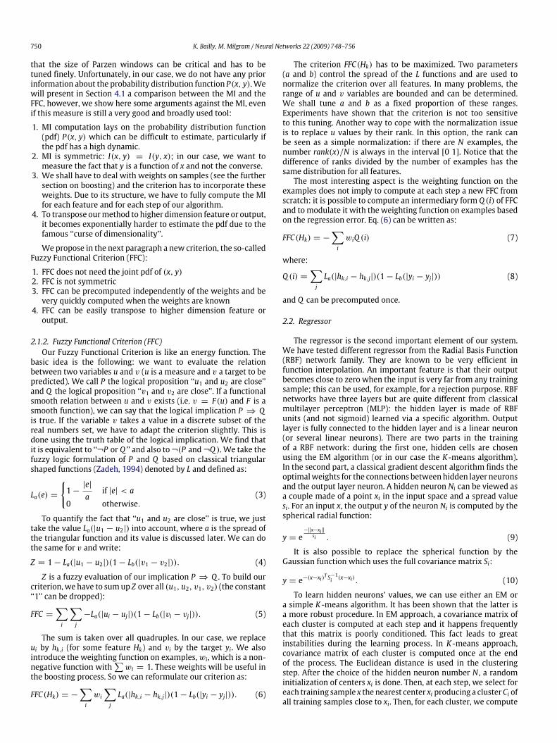
1. Initialize all examples at the same weight; FS is empty.2. Compute the fuzzy criterion for all features in F using thetraining set and the current weights. The best feature accordingto this criterion is added to FS.

3. Train a new regressor taking as input all previously selectedfeatures.

Fig. 1. BISAR algorithm.

4. Compute the new weights using the error of the regressor foreach example.

5. Repeat from 2 to 5 until the maximum number of input isreached.

6. Select the regressor with the lowest error on the validation setV during all iterations.

Hence, our method combines an iterative filtering approach forfeature selection and a neural network. The selection process usesweights provided by the network error at each step. It means that,given a set of pairs (xi, yi) of training input–output and weights onexample, we determine a new score for each feature Hk. This scorehas to reflect the relevance of featureHk for our problem, that is thematching between xi (a pattern) and yi (the target value associatedto xi that we want to predict) (Fig. 1).

2.1. Feature selection criterion

We have to determine a criterion to select features. This crite-rionmustmeasure howmuch the output ydepends functionally onthis feature Hk. Moreover, this criterion should support a weight-ing function over the example set. Usual statistical measures (cor-relations, covariance, etc.) do not fit to our situation because of thelinear hypothesis that we do not want to assume.We are going to examine two criterions: the well-known

Mutual Information (MI) and our new Fuzzy Functional Criterion(FFC) in the next sections.

2.1.1. Mutual InformationThe MI between two discrete random variables x and y is

defined to be:

I(x; y) = −∑x,y

P(x, y) log2P(x, y)P(x).P(y)

(1)

and:

I(x; y) = H(x)+ H(y)− H(x, y) = H(x)H(x|y) = H(y)H(y|x) (2)

where H(x) is the entropy of the random variable x and H(x, y) isthe joint entropy of these variables.There is a continuous definition of the MI for continuous

variables but it is necessary to approximate the MI before using itpractically in a program. So, the main problem is the estimationof the joint probability distribution function P(x, y). We use theParzen windows estimator to evaluate P(x, y) which is a popularnon-parametric approach and which is also very close to thecomputation performed by our FFC criterion. It is well known

750 K. Bailly, M. Milgram / Neural Networks 22 (2009) 748–756

that the size of Parzen windows can be critical and has to betuned finely. Unfortunately, in our case, we do not have any priorinformation about the probability distribution function P(x, y). Wewill present in Section 4.1 a comparison between the MI and theFFC, however, we show here some arguments against the MI, evenif this measure is still a very good and broadly used tool:

1. MI computation lays on the probability distribution function(pdf) P(x, y) which can be difficult to estimate, particularly ifthe pdf has a high dynamic.

2. MI is symmetric: I(x, y) = I(y, x); in our case, we want tomeasure the fact that y is a function of x and not the converse.

3. We shall have to deal with weights on samples (see the furthersection on boosting) and the criterion has to incorporate theseweights. Due to its structure, we have to fully compute the MIfor each feature and for each step of our algorithm.

4. To transpose ourmethod to higher dimension feature or output,it becomes exponentially harder to estimate the pdf due to thefamous ‘‘curse of dimensionality’’.

We propose in the next paragraph a new criterion, the so-calledFuzzy Functional Criterion (FFC):

1. FFC does not need the joint pdf of (x, y)2. FFC is not symmetric3. FFC can be precomputed independently of the weights and bevery quickly computed when the weights are known

4. FFC can be easily transpose to higher dimension feature oroutput.

2.1.2. Fuzzy Functional Criterion (FFC)Our Fuzzy Functional Criterion is like an energy function. The

basic idea is the following: we want to evaluate the relationbetween two variables u and v (u is a measure and v a target to bepredicted). We call P the logical proposition ‘‘u1 and u2 are close’’and Q the logical proposition ‘‘v1 and v2 are close’’. If a functionalsmooth relation between u and v exists (i.e. v = F(u) and F is asmooth function), we can say that the logical implication P ⇒ Qis true. If the variable v takes a value in a discrete subset of thereal numbers set, we have to adapt the criterion slightly. This isdone using the truth table of the logical implication. We find thatit is equivalent to ‘‘¬P or Q ’’ and also to¬(P and¬Q ). We take thefuzzy logic formulation of P and Q based on classical triangularshaped functions (Zadeh, 1994) denoted by L and defined as:

La(e) =

{1−|e|a

if |e| < a0 otherwise.

(3)

To quantify the fact that ‘‘u1 and u2 are close’’ is true, we justtake the value La(|u1 − u2|) into account, where a is the spread ofthe triangular function and its value is discussed later. We can dothe same for v and write:

Z = 1− La(|u1 − u2|)(1− Lb(|v1 − v2|)). (4)

Z is a fuzzy evaluation of our implication P ⇒ Q . To build ourcriterion,we have to sumup Z over all (u1, u2, v1, v2) (the constant‘‘1’’ can be dropped):

FFC =∑i

∑j

−La(|ui − uj|)(1− Lb(|vi − vj|)). (5)

The sum is taken over all quadruples. In our case, we replaceui by hk,i (for some feature Hk) and vi by the target yi. We alsointroduce the weighting function on examples,wi, which is a non-negative function with

∑wi = 1. These weights will be useful in

the boosting process. So we can reformulate our criterion as:

FFC(Hk) = −∑i

wi∑j

La(|hk,i − hk,j|)(1− Lb(|yi − yj|)). (6)

The criterion FFC(Hk) has to be maximized. Two parameters(a and b) control the spread of the L functions and are used tonormalize the criterion over all features. In many problems, therange of u and v variables are bounded and can be determined.We shall tune a and b as a fixed proportion of these ranges.Experiments have shown that the criterion is not too sensitiveto this tuning. Another way to cope with the normalization issueis to replace u values by their rank. In this option, the rank canbe seen as a simple normalization: if there are N examples, thenumber rank(x)/N is always in the interval [0 1]. Notice that thedifference of ranks divided by the number of examples has thesame distribution for all features.The most interesting aspect is the weighting function on the

examples does not imply to compute at each step a new FFC fromscratch: it is possible to compute an intermediary form Q (i) of FFCand tomodulate it with the weighting function on examples basedon the regression error. Eq. (6) can be written as:

FFC(Hk) = −∑i

wiQ (i) (7)

where:

Q (i) =∑j

La(|hk,i − hk,j|)(1− Lb(|yi − yj|)) (8)

and Q can be precomputed once.

2.2. Regressor

The regressor is the second important element of our system.We have tested different regressor from the Radial Basis Function(RBF) network family. They are known to be very efficient infunction interpolation. An important feature is that their outputbecomes close to zero when the input is very far from any trainingsample; this can be used, for example, for a rejection purpose. RBFnetworks have three layers but are quite different from classicalmultilayer perceptron (MLP): the hidden layer is made of RBFunits (and not sigmoid) learned via a specific algorithm. Outputlayer is fully connected to the hidden layer and is a linear neuron(or several linear neurons). There are two parts in the trainingof a RBF network: during the first one, hidden cells are chosenusing the EM algorithm (or in our case the K -means algorithm).In the second part, a classical gradient descent algorithm finds theoptimalweights for the connections betweenhidden layer neuronsand the output layer neuron. A hidden neuron Ni can be viewed asa couple made of a point xi in the input space and a spread valuesi. For an input x, the output y of the neuron Ni is computed by thespherical radial function:

y = e−‖x−xi‖si . (9)

It is also possible to replace the spherical function by theGaussian function which uses the full covariance matrix Si:

y = e−(x−xi)T S−1i (x−xi). (10)

To learn hidden neurons’ values, we can use either an EM ora simple K -means algorithm. It has been shown that the latter isa more robust procedure. In EM approach, a covariance matrix ofeach cluster is computed at each step and it happens frequentlythat this matrix is poorly conditioned. This fact leads to greatinstabilities during the learning process. In K -means approach,covariance matrix of each cluster is computed once at the endof the process. The Euclidean distance is used in the clusteringstep. After the choice of the hidden neuron number N , a randominitialization of centers xi is done. Then, at each step, we select foreach training sample x the nearest center xi producing a clusterCi ofall training samples close to xi. Then, for each cluster, we compute

K. Bailly, M. Milgram / Neural Networks 22 (2009) 748–756 751

mi the center of gravity of Ci and set xi tomi. The process runs untilxi are stable or themaximumnumber of iterations is reached. Oncehidden neurons are learned,we determine otherweights (betweenhidden and output layers) via a gradient descent to minimize theMean Square Error between desired output and network output.We also used a Generalized Regression Neural Network (GRNN)

which can be considered as a simplified RBF network (Wasserman,1993). Each center of the hidden unit corresponds to an exampleof the training set and weights between hidden and output layersare set to the target values. It means this network does not needany training step but instead just keeps all prototypes (in thehidden layer) and all targets (in the second layer weights). Thisnetwork can be viewed as a Parzen window procedure applied toan interpolation task.

2.3. Boosting strategy

At the beginning, the neural network starts with only one inputcell which corresponds to the best feature given by the criterionusing a uniform weighting function. In the second step, a newnetwork is trained with 2 input cells: the new input correspondsto the second best feature which is selected among all features(except the feature already selected) usingweights provided by theerror of the first network. It means that examples that are poorlyprocessed by the first network will receive higher weights thanothers. By doing that, we believe that the resulting weights, whenfed to the criterion computation, will lead the criterion to choosea new feature better adapted to these examples. It is clear thatour boosting paradigm enhances the regression system. Contraryto AdaBoost (Schapire, 2003), iterative reweighting is only usedto select the best complementary feature. Features combinationis entirely handled by the regressor and weights are taken intoaccount. It can be seen as a regularization to prevent overfitting.Several strategies are possible to drive the selection process.

One has to tune the weights according to the error and this weightadaptation has to be defined carefully.We test three boosting mechanisms. The first one lies on a

memoryless process. Weights at iteration t + 1 are only relatedto the quadratic error εtk at the previous iteration. In our case, weadopted this simple relation:

wt+1(i) =(εt(i))2

M∑i=1(εt(i))2

. (11)

The second boosting strategy is cumulative and the weightof each example depends on the regression model error and theprevious weights.

w̃t+1(i) ={wt(i) if εt(i) < mediani(εt(i))max {αwt(i), wmax} otherwise (12)

wt+1(i) =w̃t+1(i)

M∑i=1(w̃t+1(i))

. (13)

Weights of half the examples with the highest prediction errorare multiplied by a constant accumulation factor α. Here wmax isa constant used to avoid overfitting. Typically, α is set to 1.1 andwmax to 0.1.The third reweighting procedure is the same as in AdaBoost.R2

(Drucker, 1997). The performance of the regressor is measuredusing a loss function:

Lt(i) =

εt(i)maxi=1...M

εt(i)

2 . (14)

a b c

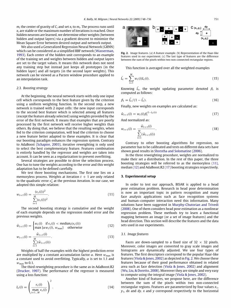
Fig. 2. Image features. (a) A feature example. (b) Representation of the Haar-likefeatures used in our experiment. (c) The last type of features are the differencebetween the sum of the pixels within two non-connected rectangular regions.

This function is averaged over all the weighted examples

L̄t =M∑i=1

wt(i)Lt(i). (15)

Knowing L̄t , the weight updating parameter denoted βt iscomputed as follows:

βt = L̄t/(1− L̄t). (16)

Finally, new weights on examples are calculated as:

w̃t+1(i) = wt(i)β(1−Lt (i))t (17)

And normalized as:

wt+1(i) =w̃t+1(i)

M∑i=1(w̃t+1(i))

. (18)

Contrary to other boosting algorithms for regression, noparameter has to be calibrated and tests on different data sets haveshown good results in Shrestha and Solomatine (2006).In the three reweighting procedure, weights are normalized to

make their set a distribution. In the rest of this paper, the threeboosting strategies will be referred to as the memoryless (11),median (12) and AdaBoost.R2 (17) boosting strategies respectively.

3. Experimental setup

In order to test our approach, BISAR is applied to a headpose estimation problem. Research in head pose determinationis now an important topic in pattern recognition and manyface analysis applications such as face recognition systemsand human–computer interaction need this information. Manysolutions have been suggested in Murphy-Chutorian and Trivedi(2008). One of them considers head pose estimation as a nonlinearregression problem. These methods try to learn a functionalmapping between an image (or a set of image features) and thehead direction. This section will describe the features and the datasets used in our experiments.

3.1. Image features

Faces are down-sampled to a fixed size of 32 × 32 pixels.Moreover, color images are converted to gray scale images andhistograms are dynamically adjusted. We use four types offeatures. The first descriptors correspond to the popular Haar-likefeatures (Viola & Jones, 2002) as depicted in Fig. 2.We choose thesefeatures because of their good performance obtained in relatedarea such as face detection (Viola & Jones, 2002) and alignment(Wu, Liu, & Doretto, 2008). Moreover they are simple and very easyto compute using the integral image (Viola & Jones, 2002).Another kind of features, we propose here, are the difference

between the sum of the pixels within two non-connectedrectangular regions. Features are parameterized by four values x1,y1, dx and dy. x and y correspond respectively to the horizontal

752 K. Bailly, M. Milgram / Neural Networks 22 (2009) 748–756

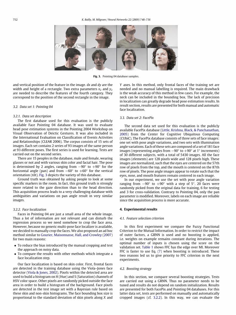
Fig. 3. Pointing 04 database samples.

and vertical position of the feature in the image. dx and dy are thewidth and height of a rectangle. Two extra parameters x2 and y2are needed to describe the features of the fourth category. Theycorrespond to the position of the second rectangle in the image.

3.2. Data set 1: Pointing 04

3.2.1. Data set descriptionThe first database used for this evaluation is the publicly

available Face Pointing 04 database. It was used to evaluatehead pose estimation systems in the Pointing 2004 Workshop onVisual Observation of Deictic Gestures. It was also included inthe International Evaluation on Classification of Events Activitiesand Relationships (CLEAR 2006). The corpus consists of 15 sets ofimages. Each set contains 2 series of 93 images of the same personat 93 different poses. The first series is used for learning. Tests arecarried out on the second series.There are 15 peoples in the database, male and female, wearing

glasses or not and with various skin color and facial hair. The poseis determined by 2 angles, ranging from −90◦ to +90◦ for thehorizontal angle (pan) and from −60◦ to +60◦ for the verticalorientation (tilt). Fig. 3 depicts the variety of this database.Ground truth was obtained by asking people to look at some

specific markers in the room. In fact, this ground truth is stronglymore related to the gaze direction than to the head direction.This acquisition process leads to a very challenging database withambiguities and variations on pan angle result in very similarimages.

3.2.2. Face localizationFaces in Pointing 04 are just a small area of the whole image.

Thus a lot of information are not relevant and can disturb theregression process so we need somehow to crop the face area.However, because no generic multi-pose face localizer is available,we decided tomanually crop the faces.We also proposed an ad hocmethod similar to Gourier, Maisonnasse, Hall, and Crowley (2007)for two main reasons:

• To reduce the bias introduced by the manual cropping and testthe approach on noisy data.• To compare the results with other methods which integrate aface localization step.

Our face localization is based on skin color. First, frontal facesare detected in the training database using the Viola–Jones facedetector (Viola & Jones, 2002). Pixels within the detected area areused to build a histogram onH (Hue) and S (Saturation) channels ofHSV color space. Other pixels are randomly picked outside the facearea in order to build a histogram of the background. Face pixelsare detected in the test image set with a Bayesian rule based onthese skin and non-skin histograms. The face bounding box size isproportional to the standard deviation of skin pixels along X and

Y axes. In this method, only frontal faces of the training set areneeded and no manual labelling is required. The main drawbackis the weak accuracy of this method in few cases. For example, theneck can be included in the bounding box. The lack of precisionin localization can greatly degrade head pose estimation results. Inresult section, results are presented for bothmanual and automaticface localization.

3.3. Data set 2: FacePix

The second data set used for this evaluation is the publiclyavailable FacePix database (Little, Krishna, Black, & Panchanathan,2005) from the Center for Cognitive Ubiquitous Computing(CUbiC). The FacePix database consists of three sets of face images:one set with pose angle variations, and two sets with illuminationangle variations. Each of these sets are composed of a set of 181 faceimages (representing angles from−90◦ to+90◦ at 1◦ increments)of 30 different subjects, with a total of 5430 images. All the faceimages (elements) are 128 pixels wide and 128 pixels high. Theseimages are normalized, such that the eyes are centered on the 57throw of pixels from the top, and the mouth is centered on the 87throw of pixels. The pose angle images appear to rotate such that theeyes, nose, and mouth features remain centered in each image.In our experiment, we use the set with pose angle variation

ranging from −90◦ to +90◦ with a step of 5◦. 20 faces wererandomly picked from the original data for training, 6 for testingand 3 for cross-validation. Contrary to Pointing 04, only the panparameter is modified. Moreover, labels on each image are reliablesince the acquisition process is more accurate.

4. Experimental results

4.1. Feature selection criterion

In this first experiment we compare the Fuzzy FunctionalCriterion to the Mutual Information. In order to restrict the impactof outer factors, a GRNN is used and no boosting is applied,i.e. weights on example remains constant during iterations. Theoptimal number of inputs is chosen using the score on thevalidation set. Table 1 shows FFC has the edge over MI. MoreoverFFC is faster to use Eq. (7) when boosting is introduced. Thesetwo reasons led us to give priority to FFC criterion in the nextexperiments.

4.2. Boosting strategy

In this section, we compare several boosting strategies. Testsare carried out using a GRNN. Thus no parameter needs to betuned and results do not depend on random initialization. Resultsare presented for both FacePix and Pointing 04 databases. For thislatter data set, tests are performed on manually and automaticallycropped images (cf. 3.2.2). In this way, we can evaluate the

K. Bailly, M. Milgram / Neural Networks 22 (2009) 748–756 753

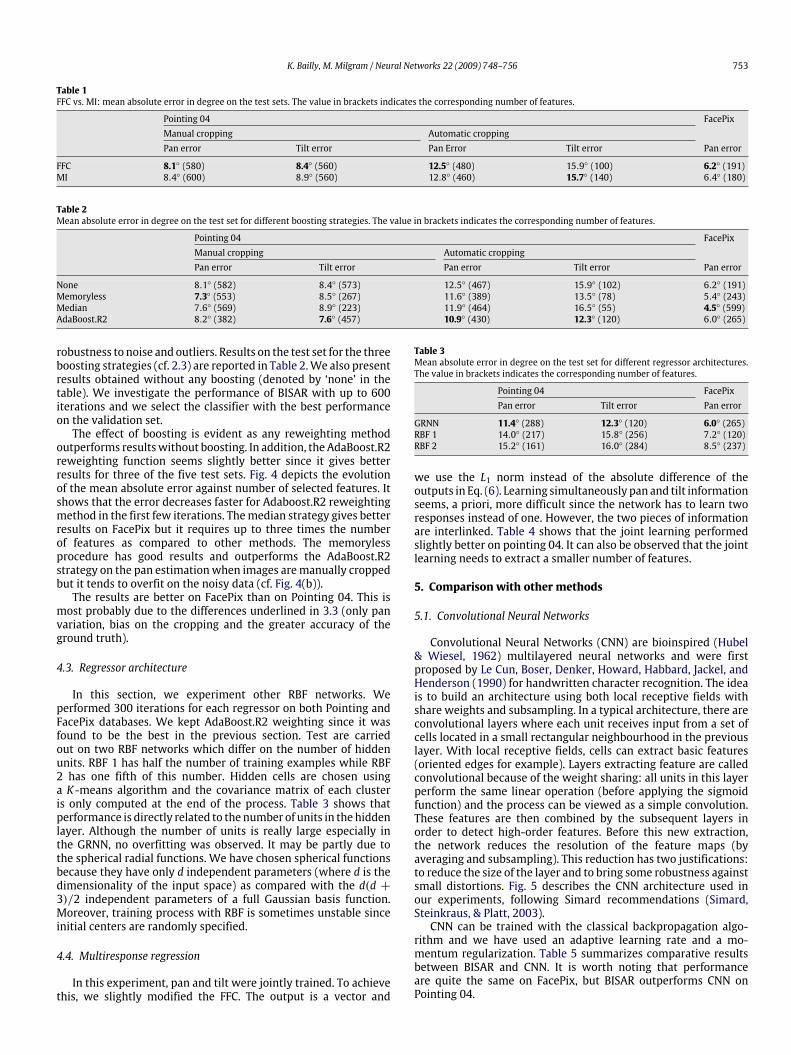
Table 1FFC vs. MI: mean absolute error in degree on the test sets. The value in brackets indicates the corresponding number of features.

Pointing 04 FacePixManual cropping Automatic croppingPan error Tilt error Pan Error Tilt error Pan error

FFC 8.1◦ (580) 8.4◦ (560) 12.5◦ (480) 15.9◦ (100) 6.2◦ (191)MI 8.4◦ (600) 8.9◦ (560) 12.8◦ (460) 15.7◦ (140) 6.4◦ (180)

Table 2Mean absolute error in degree on the test set for different boosting strategies. The value in brackets indicates the corresponding number of features.

Pointing 04 FacePixManual cropping Automatic croppingPan error Tilt error Pan error Tilt error Pan error

None 8.1◦ (582) 8.4◦ (573) 12.5◦ (467) 15.9◦ (102) 6.2◦ (191)Memoryless 7.3◦ (553) 8.5◦ (267) 11.6◦ (389) 13.5◦ (78) 5.4◦ (243)Median 7.6◦ (569) 8.9◦ (223) 11.9◦ (464) 16.5◦ (55) 4.5◦ (599)AdaBoost.R2 8.2◦ (382) 7.6◦ (457) 10.9◦ (430) 12.3◦ (120) 6.0◦ (265)

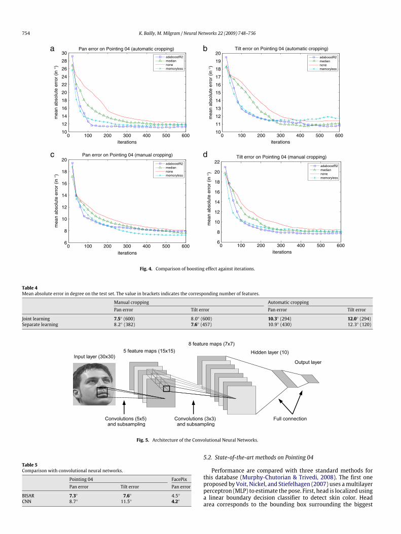
robustness to noise and outliers. Results on the test set for the threeboosting strategies (cf. 2.3) are reported in Table 2.We also presentresults obtained without any boosting (denoted by ‘none’ in thetable). We investigate the performance of BISAR with up to 600iterations and we select the classifier with the best performanceon the validation set.The effect of boosting is evident as any reweighting method

outperforms resultswithout boosting. In addition, the AdaBoost.R2reweighting function seems slightly better since it gives betterresults for three of the five test sets. Fig. 4 depicts the evolutionof the mean absolute error against number of selected features. Itshows that the error decreases faster for Adaboost.R2 reweightingmethod in the first few iterations. Themedian strategy gives betterresults on FacePix but it requires up to three times the numberof features as compared to other methods. The memorylessprocedure has good results and outperforms the AdaBoost.R2strategy on the pan estimationwhen images aremanually croppedbut it tends to overfit on the noisy data (cf. Fig. 4(b)).The results are better on FacePix than on Pointing 04. This is

most probably due to the differences underlined in 3.3 (only panvariation, bias on the cropping and the greater accuracy of theground truth).

4.3. Regressor architecture

In this section, we experiment other RBF networks. Weperformed 300 iterations for each regressor on both Pointing andFacePix databases. We kept AdaBoost.R2 weighting since it wasfound to be the best in the previous section. Test are carriedout on two RBF networks which differ on the number of hiddenunits. RBF 1 has half the number of training examples while RBF2 has one fifth of this number. Hidden cells are chosen usinga K -means algorithm and the covariance matrix of each clusteris only computed at the end of the process. Table 3 shows thatperformance is directly related to the number of units in the hiddenlayer. Although the number of units is really large especially inthe GRNN, no overfitting was observed. It may be partly due tothe spherical radial functions. We have chosen spherical functionsbecause they have only d independent parameters (where d is thedimensionality of the input space) as compared with the d(d +3)/2 independent parameters of a full Gaussian basis function.Moreover, training process with RBF is sometimes unstable sinceinitial centers are randomly specified.

4.4. Multiresponse regression

In this experiment, pan and tilt were jointly trained. To achievethis, we slightly modified the FFC. The output is a vector and

Table 3Mean absolute error in degree on the test set for different regressor architectures.The value in brackets indicates the corresponding number of features.

Pointing 04 FacePixPan error Tilt error Pan error

GRNN 11.4◦ (288) 12.3◦ (120) 6.0◦ (265)RBF 1 14.0◦ (217) 15.8◦ (256) 7.2◦ (120)RBF 2 15.2◦ (161) 16.0◦ (284) 8.5◦ (237)

we use the L1 norm instead of the absolute difference of theoutputs in Eq. (6). Learning simultaneously pan and tilt informationseems, a priori, more difficult since the network has to learn tworesponses instead of one. However, the two pieces of informationare interlinked. Table 4 shows that the joint learning performedslightly better on pointing 04. It can also be observed that the jointlearning needs to extract a smaller number of features.

5. Comparison with other methods

5.1. Convolutional Neural Networks

Convolutional Neural Networks (CNN) are bioinspired (Hubel& Wiesel, 1962) multilayered neural networks and were firstproposed by Le Cun, Boser, Denker, Howard, Habbard, Jackel, andHenderson (1990) for handwritten character recognition. The ideais to build an architecture using both local receptive fields withshare weights and subsampling. In a typical architecture, there areconvolutional layers where each unit receives input from a set ofcells located in a small rectangular neighbourhood in the previouslayer. With local receptive fields, cells can extract basic features(oriented edges for example). Layers extracting feature are calledconvolutional because of the weight sharing: all units in this layerperform the same linear operation (before applying the sigmoidfunction) and the process can be viewed as a simple convolution.These features are then combined by the subsequent layers inorder to detect high-order features. Before this new extraction,the network reduces the resolution of the feature maps (byaveraging and subsampling). This reduction has two justifications:to reduce the size of the layer and to bring some robustness againstsmall distortions. Fig. 5 describes the CNN architecture used inour experiments, following Simard recommendations (Simard,Steinkraus, & Platt, 2003).CNN can be trained with the classical backpropagation algo-

rithm and we have used an adaptive learning rate and a mo-mentum regularization. Table 5 summarizes comparative resultsbetween BISAR and CNN. It is worth noting that performanceare quite the same on FacePix, but BISAR outperforms CNN onPointing 04.

754 K. Bailly, M. Milgram / Neural Networks 22 (2009) 748–756

0 100 200 300 400 500 60010

12

14

16

18

20

22

24

26

28

30

iterations0 100 200 300 400 500 600

iterations

0 100 200 300 400 500 600iterations

mea

n ab

solu

te e

rror

(in

°)

Pan error on Pointing 04 (automatic cropping)

adaboostR2mediannonememoryless

10

11

12

13

14

15

16

17

18

19

20

mea

n ab

solu

te e

rror

(in

°)

Tilt error on Pointing 04 (automatic cropping)

adaboostR2mediannonememoryless

0 100 200 300 400 500 6006

8

10

12

14

16

18

20

iterations

mea

n ab

solu

te e

rror

(in

°)

Pan error on Pointing 04 (manual cropping)

adaboostR2mediannonememoryless

6

8

10

12

14

16

18

20

22

mea

n ab

solu

te e

rror

(in

°)

Tilt error on Pointing 04 (manual cropping)

adaboostR2mediannonememoryless

a b

c d

Fig. 4. Comparison of boosting effect against iterations.

Table 4Mean absolute error in degree on the test set. The value in brackets indicates the corresponding number of features.

Manual cropping Automatic croppingPan error Tilt error Pan error Tilt error

Joint learning 7.5◦ (600) 8.0◦ (600) 10.3◦ (294) 12.0◦ (294)Separate learning 8.2◦ (382) 7.6◦ (457) 10.9◦ (430) 12.3◦ (120)

Fig. 5. Architecture of the Convolutional Neural Networks.

Table 5Comparison with convolutional neural networks.

Pointing 04 FacePixPan error Tilt error Pan error

BISAR 7.3◦ 7.6◦ 4.5◦CNN 8.7◦ 11.5◦ 4.2◦

5.2. State-of-the-art methods on Pointing 04

Performance are compared with three standard methods forthis database (Murphy-Chutorian & Trivedi, 2008). The first oneproposed by Voit, Nickel, and Stiefelhagen (2007) uses amultilayerperceptron (MLP) to estimate the pose. First, head is localized usinga linear boundary decision classifier to detect skin color. Headarea corresponds to the bounding box surrounding the biggest

K. Bailly, M. Milgram / Neural Networks 22 (2009) 748–756 755

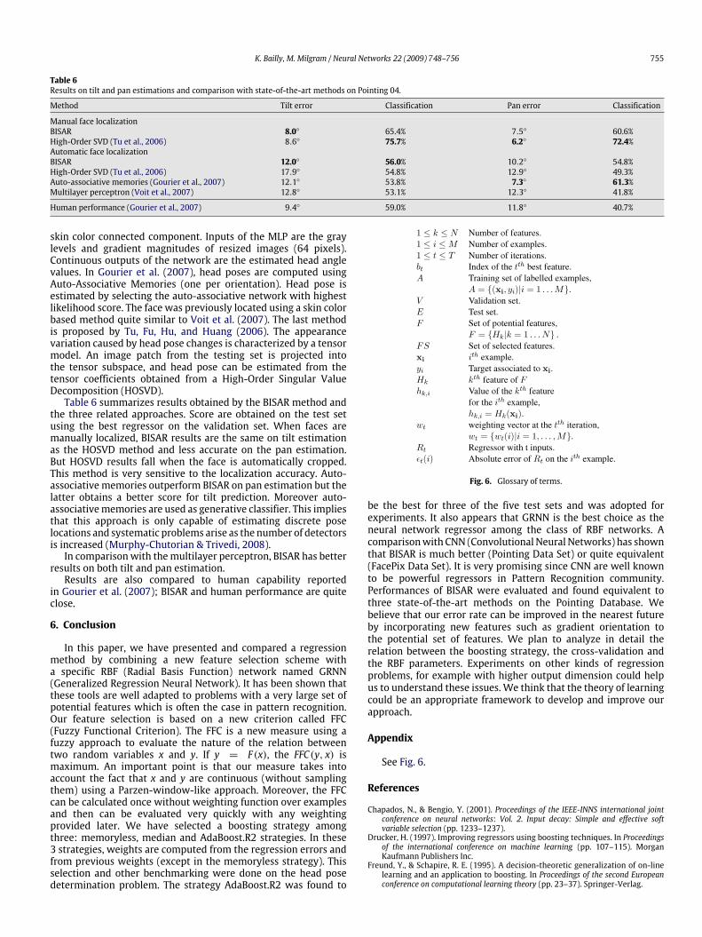
Table 6Results on tilt and pan estimations and comparison with state-of-the-art methods on Pointing 04.

Method Tilt error Classification Pan error Classification

Manual face localizationBISAR 8.0◦ 65.4% 7.5◦ 60.6%High-Order SVD (Tu et al., 2006) 8.6◦ 75.7% 6.2◦ 72.4%Automatic face localizationBISAR 12.0◦ 56.0% 10.2◦ 54.8%High-Order SVD (Tu et al., 2006) 17.9◦ 54.8% 12.9◦ 49.3%Auto-associative memories (Gourier et al., 2007) 12.1◦ 53.8% 7.3◦ 61.3%Multilayer perceptron (Voit et al., 2007) 12.8◦ 53.1% 12.3◦ 41.8%

Human performance (Gourier et al., 2007) 9.4◦ 59.0% 11.8◦ 40.7%

skin color connected component. Inputs of the MLP are the graylevels and gradient magnitudes of resized images (64 pixels).Continuous outputs of the network are the estimated head anglevalues. In Gourier et al. (2007), head poses are computed usingAuto-Associative Memories (one per orientation). Head pose isestimated by selecting the auto-associative network with highestlikelihood score. The face was previously located using a skin colorbased method quite similar to Voit et al. (2007). The last methodis proposed by Tu, Fu, Hu, and Huang (2006). The appearancevariation caused by head pose changes is characterized by a tensormodel. An image patch from the testing set is projected intothe tensor subspace, and head pose can be estimated from thetensor coefficients obtained from a High-Order Singular ValueDecomposition (HOSVD).Table 6 summarizes results obtained by the BISAR method and

the three related approaches. Score are obtained on the test setusing the best regressor on the validation set. When faces aremanually localized, BISAR results are the same on tilt estimationas the HOSVD method and less accurate on the pan estimation.But HOSVD results fall when the face is automatically cropped.This method is very sensitive to the localization accuracy. Auto-associative memories outperform BISAR on pan estimation but thelatter obtains a better score for tilt prediction. Moreover auto-associativememories are used as generative classifier. This impliesthat this approach is only capable of estimating discrete poselocations and systematic problems arise as the number of detectorsis increased (Murphy-Chutorian & Trivedi, 2008).In comparisonwith themultilayer perceptron, BISAR has better

results on both tilt and pan estimation.Results are also compared to human capability reported

in Gourier et al. (2007); BISAR and human performance are quiteclose.

6. Conclusion

In this paper, we have presented and compared a regressionmethod by combining a new feature selection scheme witha specific RBF (Radial Basis Function) network named GRNN(Generalized Regression Neural Network). It has been shown thatthese tools are well adapted to problems with a very large set ofpotential features which is often the case in pattern recognition.Our feature selection is based on a new criterion called FFC(Fuzzy Functional Criterion). The FFC is a new measure using afuzzy approach to evaluate the nature of the relation betweentwo random variables x and y. If y = F(x), the FFC(y, x) ismaximum. An important point is that our measure takes intoaccount the fact that x and y are continuous (without samplingthem) using a Parzen-window-like approach. Moreover, the FFCcan be calculated once without weighting function over examplesand then can be evaluated very quickly with any weightingprovided later. We have selected a boosting strategy amongthree: memoryless, median and AdaBoost.R2 strategies. In these3 strategies, weights are computed from the regression errors andfrom previous weights (except in the memoryless strategy). Thisselection and other benchmarking were done on the head posedetermination problem. The strategy AdaBoost.R2 was found to

Fig. 6. Glossary of terms.

be the best for three of the five test sets and was adopted forexperiments. It also appears that GRNN is the best choice as theneural network regressor among the class of RBF networks. Acomparisonwith CNN (Convolutional Neural Networks) has shownthat BISAR is much better (Pointing Data Set) or quite equivalent(FacePix Data Set). It is very promising since CNN are well knownto be powerful regressors in Pattern Recognition community.Performances of BISAR were evaluated and found equivalent tothree state-of-the-art methods on the Pointing Database. Webelieve that our error rate can be improved in the nearest futureby incorporating new features such as gradient orientation tothe potential set of features. We plan to analyze in detail therelation between the boosting strategy, the cross-validation andthe RBF parameters. Experiments on other kinds of regressionproblems, for example with higher output dimension could helpus to understand these issues. We think that the theory of learningcould be an appropriate framework to develop and improve ourapproach.

Appendix

See Fig. 6.

References

Chapados, N., & Bengio, Y. (2001). Proceedings of the IEEE-INNS international jointconference on neural networks: Vol. 2. Input decay: Simple and effective softvariable selection (pp. 1233–1237).

Drucker, H. (1997). Improving regressors using boosting techniques. In Proceedingsof the international conference on machine learning (pp. 107–115). MorganKaufmann Publishers Inc.

Freund, Y., & Schapire, R. E. (1995). A decision-theoretic generalization of on-linelearning and an application to boosting. In Proceedings of the second Europeanconference on computational learning theory (pp. 23–37). Springer-Verlag.

756 K. Bailly, M. Milgram / Neural Networks 22 (2009) 748–756

Gourier, N., Maisonnasse, J., Hall, D., & Crowley, J. L. (2007). Head pose estimation onlow resolution images. In LNCS,Multimodal technologies for perception of humans(pp. 270–280). Springer.

Guyon, I., & Elisseeff, A. (2003). An introduction to variable and feature selection.Journal of Machine Learning Research, 3, 1157–1182.

Hubel, D., &Wiesel, T. (1962). Receptive fields, binocular interaction, and functionalarchitecture in the cat’s visual cortex. J. Physiology, 160, 106–154.

Kohavi, R., & John, G. H. (1997). Wrappers for feature subset selection. ArtificialIntelligence, 97(1–2), 273–324.

Le Cun, Y., Boser, B., Denker, J. S., Howard, R. E., Habbard,W., Jackel, L. D., et al. (1990)Handwritten digit recognition with a back-propagation network. (pp. 396–404).

Little, G., Krishna, S., Black, J., & Panchanathan, S. (2005). A methodology forevaluating robustness of face recognition algorithms with respect to variationsin pose angle and illumination angle. In Proceedings of the IEEE internationalconference on acoustics, speech and signal processing .

Murphy-Chutorian, E., & Trivedi, M. (2008). Head pose estimation in computervision: A survey. IEEE Transactions on PAMI , 99.

Redpath, D.B., & Lebart, K. (2005). Boosting feature selection. In Proceedings of theinternational conference on advances in pattern recognition (pp. 305–314).

Schapire, R. E. (2003). The boosting approach to machine learning: An overview.In D. D. Denison, M. H. Hansen, C. Holmes, B. Mallick, & B. Yu (Eds.), Nonlinearestimation and classification. Springer.

Shrestha, D. L., & Solomatine, D. P. (2006). Experiments with adaboost.rt,an improved boosting scheme for regression. Neural Computation, 18(7),1678–1710.

Simard, P.Y., Steinkraus, D., & Platt, J.C. (2003). Best practices for convolutionalneural networks applied to visual document analysis. In Proceedings of theinternational conference on document analysis and recognition (pp. 958–962).

Tibshirani, R. (1996). Regression shrinkage and selection via the lasso. Journal of theRoyal Statistical Society, Series B, 58, 267–288.

Tu, J., Fu, Y., Hu, Y., & Huang, T. S. (2006). Evaluation of head pose estimationfor studio data. In LNCS, Multimodal technologies for perception of humans(pp. 281–290).

Viola, P., & Jones, M. (2002). Robust real-time object detection. International Journalof Computer Vision.

Voit, M., Nickel, K., & Stiefelhagen, R. (2007). Neural network-based headpose estimation and multi-view fusion. In LNCS, Multimodal technologies forperception of humans (pp. 291–298). Springer.

Wasserman, P. D. (1993).Advancedmethods in neural computing. NewYork, NY, USA:John Wiley & Sons, Inc.

Wu, H., Liu, X., & Doretto, G. (2008). Face alignment via boosted ranking model.In Computer vision and pattern recognition, CVPR 2008. IEEE Conference on.(pp. 1–8).

Xu, X., & Zhang, A. (2006). Boost feature subset selection: A new gene selectionalgorithm for microarray dataset. In International conference on computationalscience: vol. 2 (pp. 670–677).

Zadeh, L. A. (1994). Soft computing and fuzzy logic. IEEE Software, 11(6), 48–56.

Kevin Bailly is a Ph.D. student at the Institute of Intelligent Systems and Robotics(ISIR), and a temporary assistant professor at Pierre and Marie Curie University(UPMC Paris 6), Paris, France. He holds an Engineering degree from the IMAC’sEngineering School and aM.Sc. in Computer Science from theUniversity of Paris-Est.His main areas of research are pattern recognition, computer vision and machinelearning.

Maurice Milgram is born in 1948 in Paris and obtained the Agrégation ofMathematics in 1971 and a Ph.D. from UTC on Probabilistic Automata Networksin 1981. He started as Assistant Professor at Technology University of Compiegne(1973) then he became full Professor (1983) at ENSEA and joined the RoboticLaboratory of the Pierre and Marie Curie University in Paris in 1986. He foundedthe PARC Laboratory which is now part of the ISIR in 1992. He has supervised about30 Ph.D. theses and 20 industrial contracts. His research interests concern PatternRecognition and Image Processing.Current work: Face localization, gaze tracking, person tracking in image

sequences, gesture recognition.Recent contracts: Person localization for a smart airbag (Faurecia), automatic

directional control of the vehicles headlampbeams (Valeo), vehicle type recognition(LPR), biometry (Sagem), on-vehicle obstacle detection (PSA), baby gaze tracking(Necker Hospital).