boolean property encoding for local set pattern discovery ... · boolean property encoding for...
TRANSCRIPT
Boolean Property Encoding for Local Set
Pattern Discovery: An Application to GeneExpression Data Analysis
Ruggero G. Pensa and Jean-Francois Boulicaut
INSA LyonLIRIS CNRS UMR 5205
F-69621 Villeurbanne cedex, France{Ruggero.Pensa,Jean-Francois.Boulicaut}@insa-lyon.fr
Abstract. In the domain of gene expression data analysis, several re-searchers have recently emphasized the promising application of localpattern (e.g., association rules, closed sets) discovery techniques fromboolean matrices that encode gene properties. Detecting local patternsby means of complete constraint-based mining techniques turns to be animportant complementary approach or invaluable counterpart to heuris-tic global model mining. To take the most from local set pattern miningapproaches, a needed step concerns gene expression property encoding(e.g., over-expression). The impact of this preprocessing phase on boththe quantity and the quality of the extracted patterns is crucial. In thispaper, we study the impact of discretization techniques by a sound com-parison between the dendrograms, i.e., trees that are generated by ahierarchical clustering algorithm on raw numerical expression data andits various derived boolean matrices. Thanks to a new similarity measure,we can select the boolean property encoding technique which preservessimilarity structures holding in the raw data. The discussion relies on sev-eral experimental results for three gene expression data sets. We believeour framework is an interesting direction of work for the many applica-tion domains in which (a) local set patterns have been proved useful, and(b) Boolean properties have to be derived from raw numerical data.
1 Introduction
This volume is dedicated to local pattern detection. It has been motivated by theneed for a better characterization of what is local pattern detection and whatare the main research challenges in this area. We contribute to this objective byconsidering the exciting application domain of transcription module discoveryfrom gene expression data. In this molecular biology context, the goal is toidentify sets of genes which seem to be co-regulated, associated with the sets ofbiological situation which seems to trigger the co-regulation.
The state-of-the-art is that global patterns like partitions can provide someuseful information and suggest some of the transcription modules. We are how-ever interested by the intrinsic limitations of these approaches, e.g., their heuris-tic nature or the lack of unexpectedness of the findings. We strongly believe
K. Morik et al. (Eds.): Local Pattern Detection, LNAI 3539, pp. 115–134, 2005.c© Springer-Verlag Berlin Heidelberg 2005
116 Ruggero G. Pensa and Jean-Francois Boulicaut
that complete extractions of local patterns which satisfy a given conjunction ofconstraints (e.g., a minimal frequency constraint or a maximality constraint) arean invaluable and complementary approach to suggest unexpected but relevantpatterns, i.e., putative transcription modules.
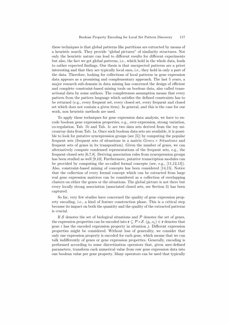
Let us now introduce the application domain and our contribution. Thanksto a huge research effort and technological breakthroughs, one of the challengesfor molecular biologists is to discover knowledge from data generated at veryhigh throughput. For instance, different techniques (including microarray [1] andSAGE [2]) enable to study the simultaneous expression of (tens of) thousands ofgenes in various biological situations. The data generated by those experimentscan be seen as expression matrices in which the expression level of genes (rows)is recorded in various biological situations (columns). A toy example of somemicroarray data is the matrix in Tab. 1a.
1 2 3 4 5
a -1 6 0 12 9b 3 -2 3 -3 1c 0 5 -1 6 6d 4 -1 2 -2 -1e -3 9 1 10 6f 5 -3 3 -6 0g 4 -4 3 -7 0h -2 2 -2 8 5
1 2 3 4 5
a 0 1 0 1 1b 1 0 1 0 1c 0 1 0 1 1d 1 0 1 0 0e 0 1 0 1 1f 1 0 1 0 1g 1 0 1 0 1h 0 0 0 1 1
1 2 3 4 5
a 0 0 0 1 0b 1 0 1 0 0c 0 0 0 1 1d 1 0 0 0 0e 0 0 0 1 0f 1 0 0 0 0g 1 0 0 0 0h 0 0 0 1 0
(a) (b) (c)
Table 1. A gene expression matrix (a) with two derived boolean matrices (band c)
Once large gene expression datasets are available, biologists have to drop thetraditional one-to-one approach to gene expression data analysis and cruciallyneed for Knowledge Discovery in Databases techniques (KDD). Among the clas-sical KDD approaches, classification techniques (i.e., learning a classifier fromdata which, for example, can predict a cancer diagnosis according to individualgene expression profiles) have been intensively studied (see, e.g., [3] for a collec-tion of recent contributions). In this paper, we do not consider such problems.We are interested in descriptive techniques which provides either global patternslike partitions (clustering) or local patterns like co-regulated sets of genes and/orsets of situations.
The use of hierarchical clustering (see, e.g., [4]) is indeed quite popular amongpractitioners. Genes are grouped together according to similar expression pro-files. The same can be done on biological situations. Thanks to the appreciatedvizualization component introduced with [4], biologists can identify some puta-tive transcription modules. Practitioners do not use only hierarchical clusteringbut also most of the classical clustering techniques. A common characteristic of
Boolean Property Encoding for Local Set Pattern Discovery 117
these techniques is that global patterns like partitions are extracted by means ofa heuristic search. They provide “global pictures” of similarity structures. Notonly the heuristic nature can lead to different results for different experimentsbut also, the fact we get global patterns, i.e., which hold in the whole data, leadsto rather expected findings. Our thesis is that unexpected patterns are a prioriinteresting and that they are typically local ones, i.e., they hold in only a part ofthe data. Therefore, looking for collections of local patterns in gene expressiondata appears as a promising and complementary approach. The last 5 years, amajor research sub-domain in data mining has concerned the design of efficientand complete constraint-based mining tools on boolean data, also called trans-actional data by some authors. The completeness assumption means that everypattern from the pattern language which satisfies the defined constraints has tobe returned (e.g., every frequent set, every closed set, every frequent and closedset which does not contain a given item). In general, and this is the case for ourwork, non heuristic methods are used.
To apply these techniques for gene expression data analysis, we have to en-code boolean gene expression properties, e.g., over-expression, strong variation,co-regulation. Tab. 1b and Tab. 1c are two data sets derived from the toy mi-croarray data from Tab. 1a. Once such boolean data sets are available, it is possi-ble to look for putative synexpression groups (see [5]) by computing the popularfrequent sets (frequent sets of situations in a matrix Genes × Situations andfrequent sets of genes in its transposition). Given the number of genes, we canalternatively compute condensed representations of the frequent sets, e.g., thefrequent closed sets [6,7,8]. Deriving association rules from synexpression groupshas been studied as well [9,10]. Furthermore, putative transcription modules canbe provided by computing the so-called formal concepts (see, e.g., [11,12,13]).Also, constraint-based mining of concepts has been considered [14,15]. Noticethat the collection of every formal concept which can be extracted from largereal gene expression matrices can be considered as a collection of overlappingclusters on either the genes or the situations. The global picture is not there butevery locally strong association (associated closed sets, see Section 3) has beencaptured.
So far, very few studies have concerned the quality of gene expression prop-erty encoding, i.e., a kind of feature construction phase. This is a critical stepbecause its impact on both the quantity and the quality of the extracted patternsis crucial.
If S denotes the set of biological situations and P denotes the set of genes,the expression properties can be encoded into r ⊆ P×S. (gi, oj) ∈ r denotes thatgene i has the encoded expression property in situation j. Different expressionproperties might be considered. Without loss of generality, we consider thatonly one expression property is encoded for each gene, which means that we cantalk indifferently of genes or gene expression properties. Generally, encoding isperformed according to some discretization operators that, given user-definedparameters, transform each numerical value from raw gene expression data intoone boolean value per gene property. Many operators can be used that typically
118 Ruggero G. Pensa and Jean-Francois Boulicaut
compute thresholds from which it is possible to decide wether the true or the falsevalue must be assigned. For instance, in Tab. 1b, an over-expression propertyhas been encoded and, e.g., Genes a, c, and e are over-expressed together inSituations 2, 4 and 5.
In [16], we have proposed a method which supports the choice for a discretiza-tion technique and an informed decision about its parameters. The idea was tostudy the impact of discretization by a sound comparison between the dendro-grams (i.e., binary trees) that are generated by the same hierarchical clusteringalgorithm applied to both the raw expression data and various derived booleanmatrices. This paper is a significant extension of [16]. The framework has beenrevisited and the experimental validation have been considerably extended.
In Section 2, we refine the similarity measure introduced in [16]. It is levelindependent, and it depends for each node on its subtree structure. It can beapplied on gene and/or situation dendrograms and we introduce an aggregatedmeasure for considering both simultaneously. Section 3 is dedicated to the use ofthis similarity measure on three real gene expression data sets in order to selectan adequate discretization technique. The robustness of the approach is alsoemphasized by an a posteriori analysis of the extracted patterns in the variousboolean contexts. For this purpose, we adapt the similarity measure betweencollections of patterns introduced in [17]. In Section 4, we study further therobustness of our approach by comparing several clustering results in the rawdata. Section 5 is a short conclusion.
2 Boolean Encoding Assessment
2.1 Comparing Binary Trees
The problem of tree comparison has motivated a lot of research. Designing sim-ilarity measures between trees is difficult because it has to be defined accordingto the semantics of trees and similarities which are generally application domaindependant. For instance, considering the analysis of phylogenies, distance mea-sures between both rooted and unrooted trees have been designed to comparedifferent phylogenetic trees concerning the same set of individuals (e.g., differentspecies of animals having a common ancestor). Various distance metrics betweentrees have been proposed. The nni (nearest neighbor interchange) and the mast(maximum agreement subtree) are two of the most used metrics. nni has beenintroduced independently in [18] and [19] and its NP-completeness has beenrecently proved [20,21]. mast has been proposed in [22], and [23] describes anefficient algorithm for computing this metrics on binary trees. These two ap-proaches are tailored for the problem of comparing phylogenies where the goal isto measure some degree of isomorphism between two dendrograms representingthe same species of biological organisms.
In our data mining problem, we have sets of objects (vectors of expressionvalues for genes in various biological situations), that we want to process with ahierarchical clustering algorithm. Depending on the different discretization oper-ations on raw expression data, a same clustering algorithm working on encoded
Boolean Property Encoding for Local Set Pattern Discovery 119
boolean gene expression data can return (very) different results. We are look-ing for a method that supports the comparison of these various gene and/orsituation dendrograms obtained on boolean data w.r.t. the common referencedendrogram that has been computed from the raw data. We need to measureboth the degree of similarity of their structures and the similarity between thecontents of their associated collections of clusters. We introduced in [16] a simplemeasure which is also easy to compute. Intuitively, it depends on the number ofmatching nodes between the two trees we have to compare.
2.2 Definition of Similarity Scores
Let O = {o1, . . . , on} denote a set of n objects. Let T denote a binary tree builton O. Let L = {l1, . . . , ln} denote the set of n leaves of T associated to O forwhich, ∀i ∈ [1 . . . n] , li ≡ oi. Let B = {b1 . . . bn−1} denote the set of the n − 1nodes of T generated by a hierarchical clustering algorithm starting from L. Byconstruction, we consider bn−1 = r, where r denotes the root of T . We definethe two sets:
δ (bi) = {bj ∈ B | bj is a descendent of bi} ,τ (bi) = {lj ∈ L | lj is a descendent of bi} .
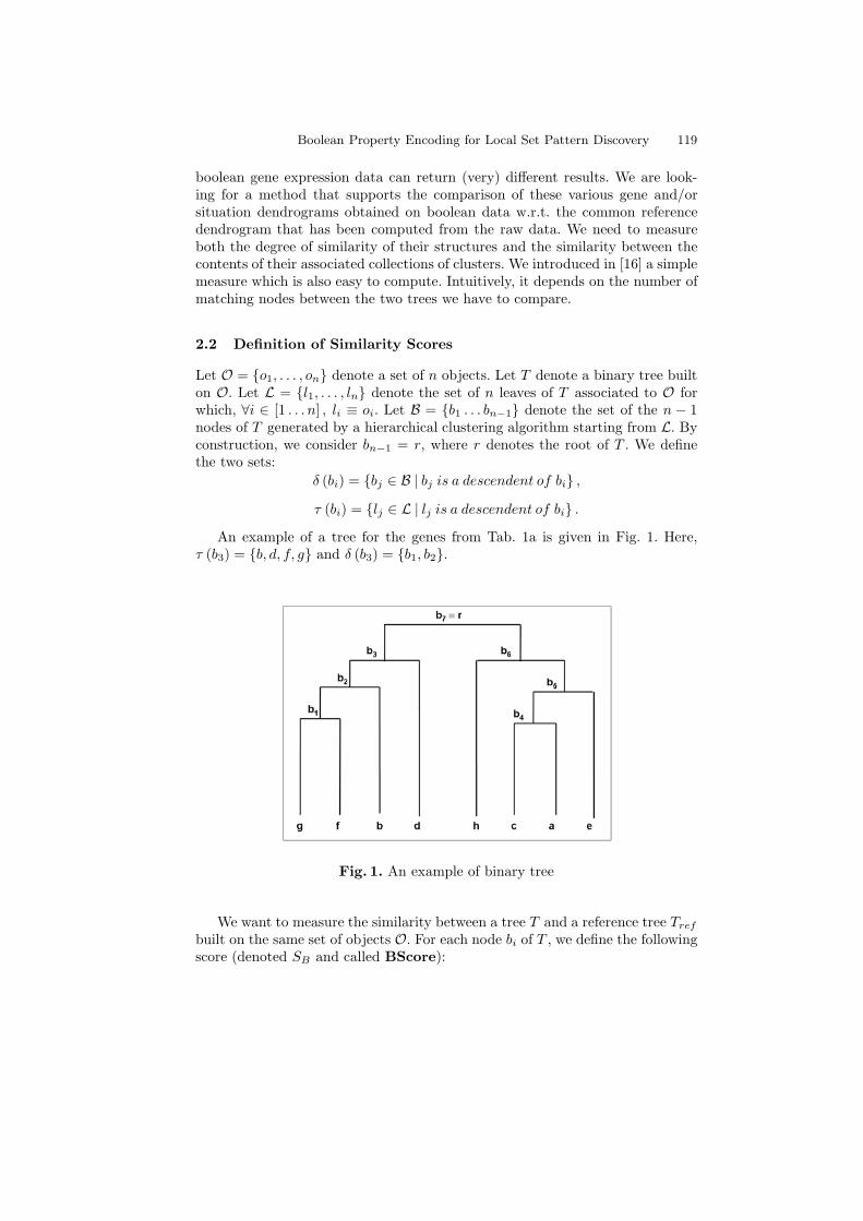
An example of a tree for the genes from Tab. 1a is given in Fig. 1. Here,τ (b3) = {b, d, f, g} and δ (b3) = {b1, b2}.
Fig. 1. An example of binary tree
We want to measure the similarity between a tree T and a reference tree Tref
built on the same set of objects O. For each node bi of T , we define the followingscore (denoted SB and called BScore):
120 Ruggero G. Pensa and Jean-Francois Boulicaut
SB (bi, Tref ) =∑
bj∈δ(bi)
aj
aj =
1|τ(bj)| , if
∃bk ∈ Tref | τ (bj) = τ (bk)0, otherwise
(1)
In other terms, for a node b in T , its score depends both on the number of itsmatching nodes in Tref (bk ∈ Tref is a matching node for b if τ (b) = τ (bk))and |τ(b)|. To obtain the similarity score of T w.r.t. Tref (denoted ST and calledTScore), we consider the BScore value on the root, i.e.:
ST (T, Tref) = SB (r, Tref ) (2)
As usually, it is interesting to normalize the measure to get a score between0 (for a tree which is totally different from the reference) and 1 (for a tree whichis equal to the reference). For the TScore measure, since its maximal valuedepends on the tree morphology, we can normalize by ST (Tref , Tref ):
ST (T, Tref) =ST (T, Tref)ST (Tref , Tref )
(3)
ST (T, Tref) = 0 means that T is totally different from Tref , i.e., there are nomatching node between T and Tref . Indeed, ST (T, Tref) = 1 means that T istotally similar to Tref , i.e., every node in T matches with a node in Tref . Giventwo trees T1 and T2 and a reference Tref , if ST (T1, Tref ) < ST (T2, Tref), thenT2 is said to be more similar to Tref than T1 according to TScore.
An important property (missing from [16]) is the following:
Property 1. The measure 1 is asymmetric, i.e. given a reference tree Tref , ∃Tsuch that ST (T, Tref) �= ST (Tref , T ).
As a consequence of this property, such a measure makes sense when one wants tocompare different binary trees with the same reference. If a symmetric measureis needed, one can consider the mean of the two possible measures for a coupleof trees:
ST (T1, T2) + ST (T2, T1)2
.
2.3 Comparison Between Gene Dendrograms
Tab. 1a is a toy example of a gene expression matrix. Each row represents a genevector, and each column represents a biological sample vector. Each cell containsan expression value for a given gene and a given sample. In this example, we haveO = {a, b, c, d, e, f, g, h}. A hierarchical clustering using the Pearson’s correlationcoefficient and the average linkage method (see, e.g., [4]) on the data from Tab. 1aleads to the dendrogram in Fig. 1.
Assume now that we discretize the expression matrix by applying two differ-ent methods used for over-expression encoding [9]. The first one, the so-called
Boolean Property Encoding for Local Set Pattern Discovery 121
“Mid-Ranged” method, considers the mean between the maximal and minimalvalues for each gene vector. Values which are greater than the average value areset to 1, 0 otherwise (Tab. 1b). A second method, the so-called “Max - X% Max”method, takes into account the maximal value for each gene vector. Values thatare greater than (100−X)% of the maximal value are set to 1, 0 otherwise. Weset X to 10 deriving the matrix in Tab. 1c.
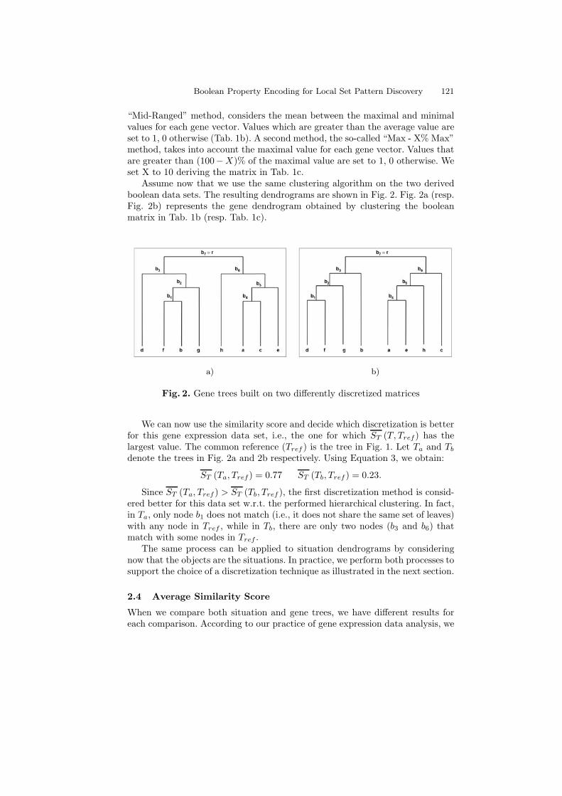
Assume now that we use the same clustering algorithm on the two derivedboolean data sets. The resulting dendrograms are shown in Fig. 2. Fig. 2a (resp.Fig. 2b) represents the gene dendrogram obtained by clustering the booleanmatrix in Tab. 1b (resp. Tab. 1c).
a) b)
Fig. 2. Gene trees built on two differently discretized matrices
We can now use the similarity score and decide which discretization is betterfor this gene expression data set, i.e., the one for which ST (T, Tref) has thelargest value. The common reference (Tref ) is the tree in Fig. 1. Let Ta and Tb
denote the trees in Fig. 2a and 2b respectively. Using Equation 3, we obtain:
ST (Ta, Tref) = 0.77 ST (Tb, Tref ) = 0.23.
Since ST (Ta, Tref ) > ST (Tb, Tref ), the first discretization method is consid-ered better for this data set w.r.t. the performed hierarchical clustering. In fact,in Ta, only node b1 does not match (i.e., it does not share the same set of leaves)with any node in Tref , while in Tb, there are only two nodes (b3 and b6) thatmatch with some nodes in Tref .
The same process can be applied to situation dendrograms by consideringnow that the objects are the situations. In practice, we perform both processes tosupport the choice of a discretization technique as illustrated in the next section.
2.4 Average Similarity Score
When we compare both situation and gene trees, we have different results foreach comparison. According to our practice of gene expression data analysis, we
122 Ruggero G. Pensa and Jean-Francois Boulicaut
often have thousands genes and a few tens or hundreds of situations. It meansthat, the similarity scores computed for situations tree are usually greater thanthose computed for gene dendrograms. This can be explained by the fact that sit-uation dendrograms have more probabilities to be identical, since they containsless leaves, and the correlation coefficients (during the hierarchical clusteringprocess) are computed on vectors of thousands components (the genes whoseexpression is measured in each situation). As a result, if we compare differentlydiscretized gene expression matrix, the discretization thresholds for which we getthe highest similarity score can be different for gene and situation dendrograms.
If we are interested in a unique similarity score, different solutions can beadopted. For example, we can consider the average between the gene and thesituation similarity scores. A problem is that if one of the trees is totally dis-similar from the reference (relative score is equal to zero), the average value willnot be zero. We can solve this problem by simply considering the square root ofthe product between the two similarity scores:
SAT (T, Tref) =√SGT (T, Tref) · SST (T, Tref) (4)
where SGT and SST and denote respectively the normalized similarity score forgenes and situation, and SAT denotes the average similarity score.
Following this definition, SAT is always between the gene and the situationsimilarity score values. Furthermore, when at least one of the two similarityscores is equal to zero, also the average similarity score is zero.
3 Using Similarity Scores
Many discretization techniques can be used to encode gene expression propertiesfrom expression values that are either integer values (case for SAGE data [2])or real values (case for microarray data [1]). In this paper, we consider for ourexperimental study only three techniques that have been used for encoding theover-expression of genes in [9]:
– “Mid-Ranged”. The highest and lowest expression values are identified foreach gene and the mid-range value is defined. For a given gene, all expressionvalues that are strictly above the mid-range value give rise to value 1, 0otherwise.
– “Max - X% Max”. The cut off is fixed w.r.t. the maximal expression valueobserved for each gene. From this value, we remove a percentage X of thisvalue. All expression values that are greater than the (100−X)% of the Maxvalue give rise to value 1, 0 otherwise.
– “X% Max”. For each gene, we consider the situations in which its level ofexpression is in X% of the highest values. These genes are assigned to value1, 0 otherwise.
We want to evaluate the relevancy of a discretization algorithm and its pa-rameters according to the preserved properties w.r.t. a hierarchical clustering of
Boolean Property Encoding for Local Set Pattern Discovery 123
the raw data. So, we have to compare the dendrograms obtained from the threedifferent boolean matrices with the reference dendrogram.
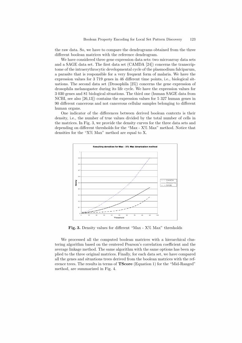
We have considered three gene expression data sets: two microarray data setsand a SAGE data set. The first data set (CAMDA [24]) concerns the transcrip-tome of the intraerythrocytic developmental cycle of the plasmodium falciparum,a parasite that is responsible for a very frequent form of malaria. We have theexpression values for 3 719 genes in 46 different time points, i.e., biological sit-uations. The second data set (Drosophila [25]) concerns the gene expression ofdrosophila melanogaster during its life cycle. We have the expression values for3 030 genes and 81 biological situations. The third one (human SAGE data fromNCBI, see also [26,13]) contains the expression values for 5 327 human genes in90 different cancerous and not cancerous cellular samples belonging to differenthuman organs.
One indicator of the differences between derived boolean contexts is theirdensity, i.e., the number of true values divided by the total number of cells inthe matrices. In Fig. 3, we provide the density curves for the three data sets anddepending on different thresholds for the “Max - X% Max” method. Notice thatdensities for the “X% Max” method are equal to X.
Fig. 3. Density values for different “Max - X% Max” thresholds
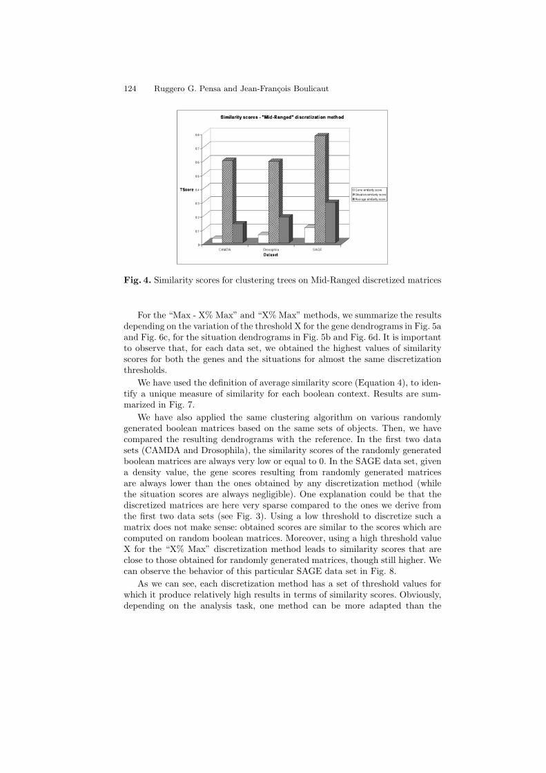
We processed all the computed boolean matrices with a hierarchical clus-tering algorithm based on the centered Pearson’s correlation coefficient and theaverage linkage method. The same algorithm with the same options has been ap-plied to the three original matrices. Finally, for each data set, we have comparedall the genes and situations trees derived from the boolean matrices with the ref-erence trees. The results in terms of TScore (Equation 1) for the “Mid-Ranged”method, are summarized in Fig. 4.
124 Ruggero G. Pensa and Jean-Francois Boulicaut
Fig. 4. Similarity scores for clustering trees on Mid-Ranged discretized matrices
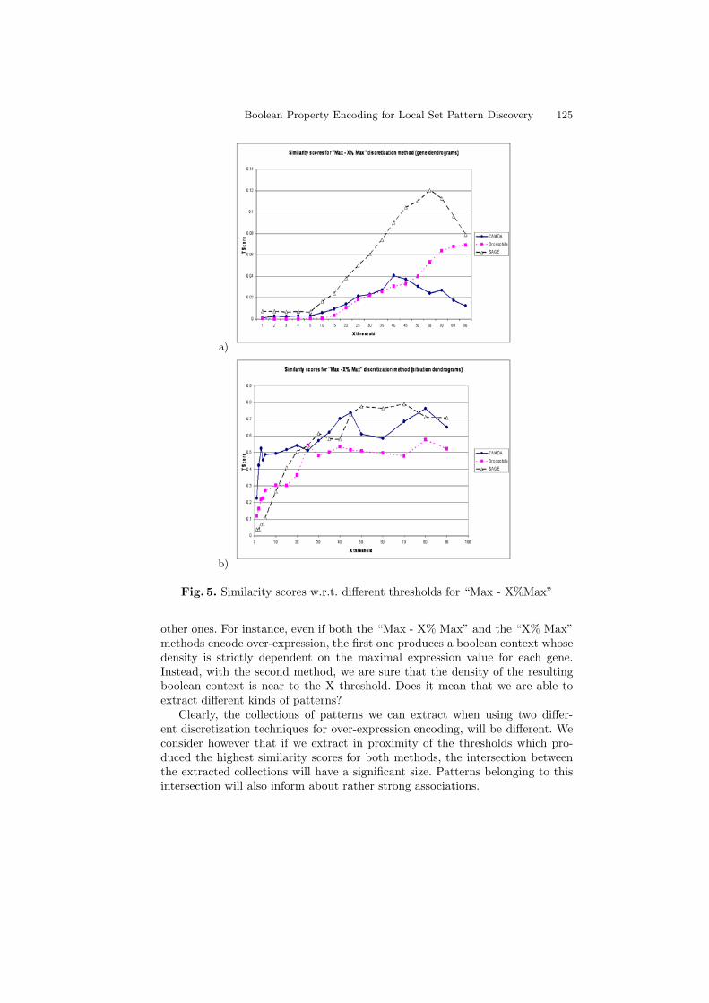
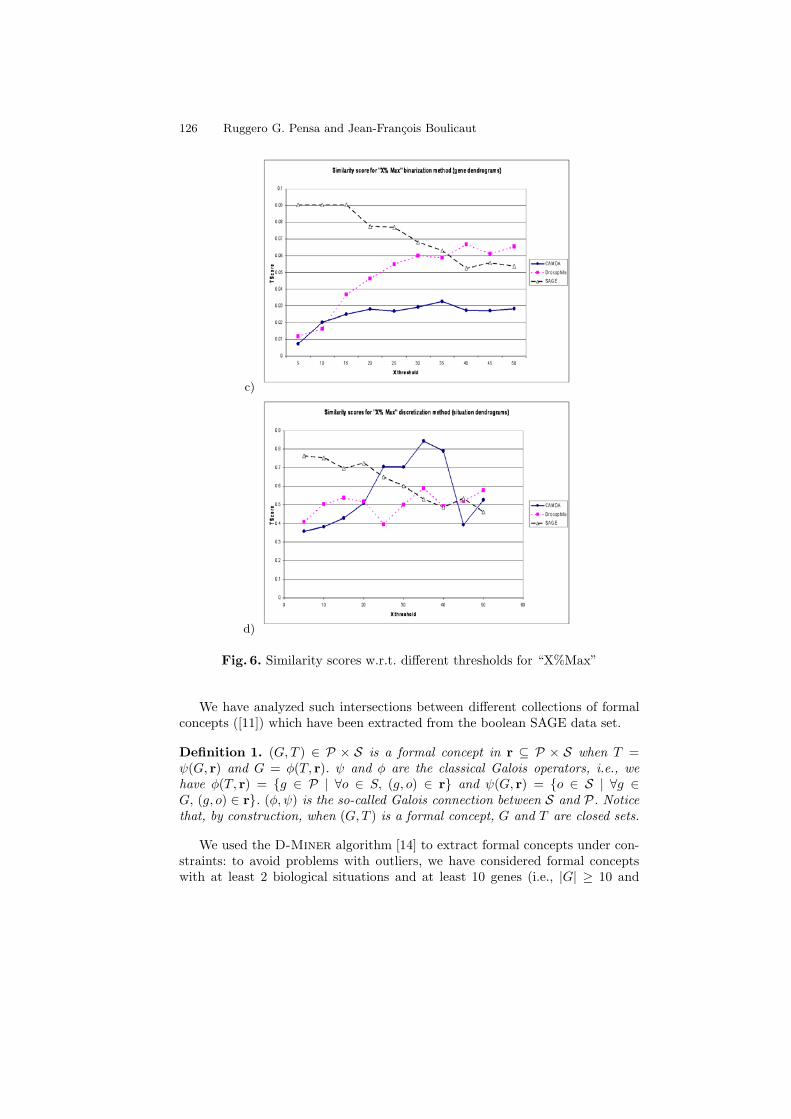
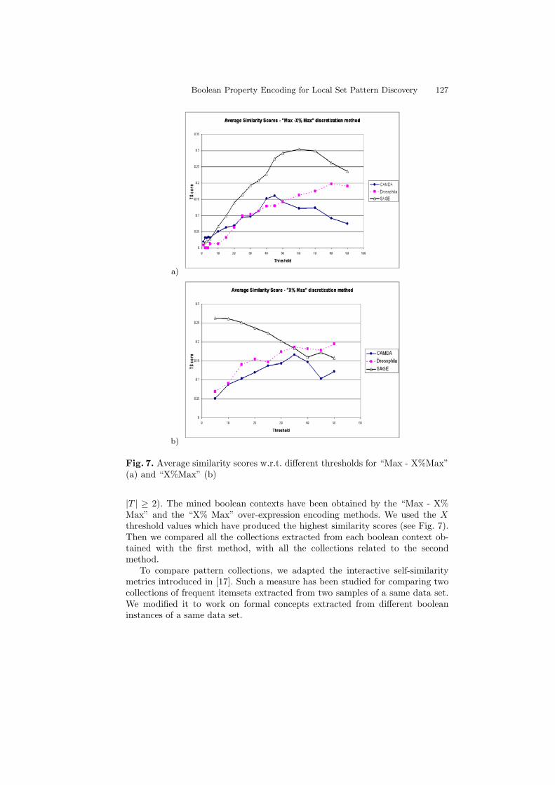
For the “Max - X% Max” and “X% Max” methods, we summarize the resultsdepending on the variation of the threshold X for the gene dendrograms in Fig. 5aand Fig. 6c, for the situation dendrograms in Fig. 5b and Fig. 6d. It is importantto observe that, for each data set, we obtained the highest values of similarityscores for both the genes and the situations for almost the same discretizationthresholds.
We have used the definition of average similarity score (Equation 4), to iden-tify a unique measure of similarity for each boolean context. Results are sum-marized in Fig. 7.
We have also applied the same clustering algorithm on various randomlygenerated boolean matrices based on the same sets of objects. Then, we havecompared the resulting dendrograms with the reference. In the first two datasets (CAMDA and Drosophila), the similarity scores of the randomly generatedboolean matrices are always very low or equal to 0. In the SAGE data set, givena density value, the gene scores resulting from randomly generated matricesare always lower than the ones obtained by any discretization method (whilethe situation scores are always negligible). One explanation could be that thediscretized matrices are here very sparse compared to the ones we derive fromthe first two data sets (see Fig. 3). Using a low threshold to discretize such amatrix does not make sense: obtained scores are similar to the scores which arecomputed on random boolean matrices. Moreover, using a high threshold valueX for the “X% Max” discretization method leads to similarity scores that areclose to those obtained for randomly generated matrices, though still higher. Wecan observe the behavior of this particular SAGE data set in Fig. 8.
As we can see, each discretization method has a set of threshold values forwhich it produce relatively high results in terms of similarity scores. Obviously,depending on the analysis task, one method can be more adapted than the
Boolean Property Encoding for Local Set Pattern Discovery 125
a)
b)
Fig. 5. Similarity scores w.r.t. different thresholds for “Max - X%Max”
other ones. For instance, even if both the “Max - X% Max” and the “X% Max”methods encode over-expression, the first one produces a boolean context whosedensity is strictly dependent on the maximal expression value for each gene.Instead, with the second method, we are sure that the density of the resultingboolean context is near to the X threshold. Does it mean that we are able toextract different kinds of patterns?
Clearly, the collections of patterns we can extract when using two differ-ent discretization techniques for over-expression encoding, will be different. Weconsider however that if we extract in proximity of the thresholds which pro-duced the highest similarity scores for both methods, the intersection betweenthe extracted collections will have a significant size. Patterns belonging to thisintersection will also inform about rather strong associations.
126 Ruggero G. Pensa and Jean-Francois Boulicaut
c)
d)
Fig. 6. Similarity scores w.r.t. different thresholds for “X%Max”
We have analyzed such intersections between different collections of formalconcepts ([11]) which have been extracted from the boolean SAGE data set.
Definition 1. (G, T ) ∈ P × S is a formal concept in r ⊆ P × S when T =ψ(G, r) and G = φ(T, r). ψ and φ are the classical Galois operators, i.e., wehave φ(T, r) = {g ∈ P | ∀o ∈ S, (g, o) ∈ r} and ψ(G, r) = {o ∈ S | ∀g ∈G, (g, o) ∈ r}. (φ, ψ) is the so-called Galois connection between S and P. Noticethat, by construction, when (G, T ) is a formal concept, G and T are closed sets.
We used the D-Miner algorithm [14] to extract formal concepts under con-straints: to avoid problems with outliers, we have considered formal conceptswith at least 2 biological situations and at least 10 genes (i.e., |G| ≥ 10 and
Boolean Property Encoding for Local Set Pattern Discovery 127
a)
b)
Fig. 7. Average similarity scores w.r.t. different thresholds for “Max - X%Max”(a) and “X%Max” (b)
|T | ≥ 2). The mined boolean contexts have been obtained by the “Max - X%Max” and the “X% Max” over-expression encoding methods. We used the Xthreshold values which have produced the highest similarity scores (see Fig. 7).Then we compared all the collections extracted from each boolean context ob-tained with the first method, with all the collections related to the secondmethod.
To compare pattern collections, we adapted the interactive self-similaritymetrics introduced in [17]. Such a measure has been studied for comparing twocollections of frequent itemsets extracted from two samples of a same data set.We modified it to work on formal concepts extracted from different booleaninstances of a same data set.

128 Ruggero G. Pensa and Jean-Francois Boulicaut
Fig. 8. Similarity scores w.r.t. density for “Max - X%Max”, “X%Max” andrandom discretization methods on SAGE data
Given two boolean contexts r1 and r2 our pattern collection similarity mea-sure is defined as follows:
Sim (C1, C2) =
∑x∈{T1}∩{T2}
|φ(x,r1)∩φ(x,r2)||φ(x,r1)∪φ(x,r2)|
|{T1} ∪ {T2}| (5)
where C1 = {(G1, T1) | (G1, T1) is a concept} and C2 = {(G2, T2) | (G2, T2) is aconcept} are the collection of concepts extracted respectively from r1 and r2.
To better understand the meaning of this measure, we can see a toy examplebased on the tables Tab. 1b and Tab. 1b. Let Cb and Cc denote the collectionof formal concepts extracted respectively from the boolean matrices in Tab. 1band Tab. 1c (with a non empty set of genes and a non empty set of situations).The list of concepts contained in the two collections is:
Cb Cc
(Gb1, Tb1) = {a, c, e}, {2, 4, 5} (Gc1, Tc1) = {c}, {4, 5}(Gb2, Tb2) = {b, f, g}, {1, 3, 5} (Gc2, Tc2) = {b}, {1, 3}(Gb3, Tb3) = {b, d, f, g}, {1, 3} (Gc3, Tc3) = {b, d, f, g}, {1}(Gb4, Tb4) = {a, c, e, h}, {4, 5} (Gc4, Tc4) = {a, c, e, h}, {4}(Gb5, Tb5) = {a, b, c, e, f, g, h}, {5}
Clearly, only two sets of situations are shared by the two collections. They areTb3 = Tc2 = {1, 3} and Tb4 = Tc1 = {4, 5}. We get the following result:
Sim (Cb, Cc) =|Gb3∩Gc2||Gb3∪Gc2| + |Gb4∩Gc1|
|Gb4∪Gc1|7
=14 + 1
4
7= 0.07
Applying such a measure to our different collections gives the results collectedin Tab. 2.
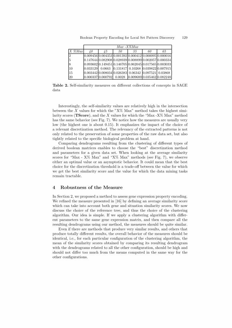
Boolean Property Encoding for Local Set Pattern Discovery 129
Max -X%Max
X %Max 40 45 50 55 60 65
2 0.009456 0.004353 0.001392 0.000412 0.000095 0.0000165 0.147644 0.082908 0.028939 0.008899 0.002057 0.0003348 0.093602 0.149451 0.146705 0.062045 0.017565 0.00303310 0.033129 0.0663 0.131817 0.10268 0.039822 0.00791515 0.003442 0.008034 0.026383 0.06342 0.097521 0.0386820 0.000337 0.000792 0.0028 0.009689 0.035462 0.082248
Table 2. Self-similarity measures on different collections of concepts in SAGEdata
Interestingly, the self-similarity values are relatively high in the intersectionbetween the X values for which the ”X% Max” method takes the highest simi-larity scores (TScore), and the X values for which the “Max -X% Max” methodhas the same behavior (see Fig. 7). We notice how the measures are usually verylow (the highest one is about 0.15). It emphasizes the impact of the choice ofa relevant discretization method. The relevancy of the extracted patterns is notonly related to the preservation of some properties of the raw data set, but alsotightly related to the specific biological problem at hand.
Comparing dendrograms resulting from the clustering of different types ofderived boolean matrices enables to choose the “best” discretization methodand parameters for a given data set. When looking at the average similarityscores for “Max - X% Max” and “X% Max” methods (see Fig. 7), we observeeither an optimal value or an asymptotic behavior. It could mean that the bestchoice for the discretization threshold is a trade-off between the value for whichwe get the best similarity score and the value for which the data mining tasksremain tractable.
4 Robustness of the Measure
In Section 2, we proposed a method to assess gene expression property encoding.We refined the measure presented in [16] by defining an average similarity scorewhich can take into account both gene and situation similarity scores. We nowdiscuss the choice of the reference tree, and thus the choice of the clusteringalgorithm. Our idea is simple. If we apply a clustering algorithm with differ-ent parameters to the same gene expression matrix, and then compare all theresulting dendrograms using our method, the measures should be quite similar.
Even if there are methods that produce very similar results, and others thatproduce totally different results, the overall behavior of the measures should beidentical, i.e., for each particular configuration of the clustering algorithm, themean of the similarity scores obtained by comparing its resulting dendrogramwith the dendrograms related to all the other configuration, should be high andshould not differ too much from the means computed in the same way for theother configurations.
130 Ruggero G. Pensa and Jean-Francois Boulicaut
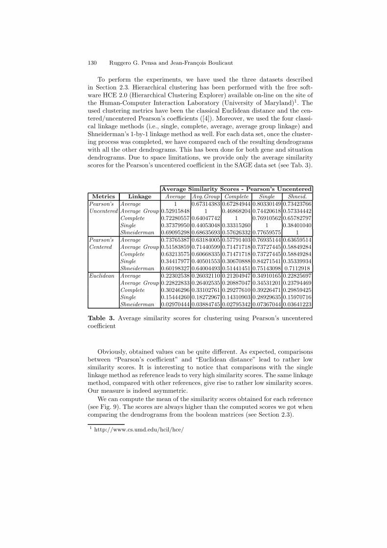
To perform the experiments, we have used the three datasets describedin Section 2.3. Hierarchical clustering has been performed with the free soft-ware HCE 2.0 (Hierarchical Clustering Explorer) available on-line on the site ofthe Human-Computer Interaction Laboratory (University of Maryland)1. Theused clustering metrics have been the classical Euclidean distance and the cen-tered/uncentered Pearson’s coefficients ([4]). Moreover, we used the four classi-cal linkage methods (i.e., single, complete, average, average group linkage) andShneiderman’s 1-by-1 linkage method as well. For each data set, once the cluster-ing process was completed, we have compared each of the resulting dendrogramswith all the other dendrograms. This has been done for both gene and situationdendrograms. Due to space limitations, we provide only the average similarityscores for the Pearson’s uncentered coefficient in the SAGE data set (see Tab. 3).
Average Similarity Scores - Pearson’s Uncentered
Metrics Linkage Average Avg.Group Complete Single Shneid.
Pearson’s Average 1 0.67314383 0.67284944 0.80330149 0.73423766Uncentered Average Group 0.52915848 1 0.46868204 0.74420618 0.57334442
Complete 0.72280557 0.64047742 1 0.76910562 0.65782797Single 0.37379950 0.44053048 0.33315260 1 0.38401040Shneiderman 0.69095298 0.68635693 0.57626332 0.77659575 1
Pearson’s Average 0.73765387 0.63184005 0.57791403 0.76935144 0.63659514Centered Average Group 0.51583859 0.71440599 0.71471718 0.73727445 0.58849284
Complete 0.63213575 0.60668335 0.71471718 0.73727445 0.58849284Single 0.34417977 0.40501553 0.30670888 0.84271541 0.35339934Shneiderman 0.60198327 0.64004493 0.51441451 0.75143098 0.7112918
Euclidean Average 0.22302538 0.26032110 0.21204947 0.34910165 0.22825697Average Group 0.22822833 0.26402535 0.20887047 0.34531201 0.23794469Complete 0.30246296 0.33102761 0.29277610 0.39226471 0.29859425Single 0.15444260 0.18272967 0.14310903 0.28929635 0.15970716Shneiderman 0.02970444 0.03884745 0.02795342 0.07367044 0.03641223
Table 3. Average similarity scores for clustering using Pearson’s uncenteredcoefficient
Obviously, obtained values can be quite different. As expected, comparisonsbetween “Pearson’s coefficient” and “Euclidean distance” lead to rather lowsimilarity scores. It is interesting to notice that comparisons with the singlelinkage method as reference leads to very high similarity scores. The same linkagemethod, compared with other references, give rise to rather low similarity scores.Our measure is indeed asymmetric.
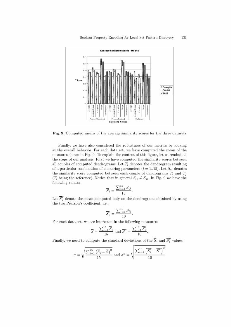
We can compute the mean of the similarity scores obtained for each reference(see Fig. 9). The scores are always higher than the computed scores we got whencomparing the dendrograms from the boolean matrices (see Section 2.3).
1 http://www.cs.umd.edu/hcil/hce/
Boolean Property Encoding for Local Set Pattern Discovery 131
Fig. 9. Computed means of the average similarity scores for the three datasets
Finally, we have also considered the robustness of our metrics by lookingat the overall behavior. For each data set, we have computed the mean of themeasures shown in Fig. 9. To explain the content of this figure, let us remind allthe steps of our analysis. First we have computed the similarity scores betweenall couples of computed dendrograms. Let Ti denotes the dendrogram resultingof a particular combination of clustering parameters (i = 1..15). Let Sij denotesthe similarity score computed between each couple of dendrograms Ti and Tj
(Ti being the reference). Notice that in general Sij �= Sji. In Fig. 9 we have thefollowing values:
Si =
∑15j=1 Sij
15.
Let Sp
i denote the mean computed only on the dendrograms obtained by usingthe two Pearson’s coefficient, i.e.,
Sp
i =
∑10j=1 Sij
10.
For each data set, we are interested in the following measures:
S =∑15
i=1 Si
15and S
p=
∑10i=1 S
p
i
10.
Finally, we need to compute the standard deviations of the Si and Sp
i values:
σ =
√∑15i=1
(Si − S
)2
15and σp =
√√√√∑10
i=1
(S
p
i − Sp)2
10
132 Ruggero G. Pensa and Jean-Francois Boulicaut
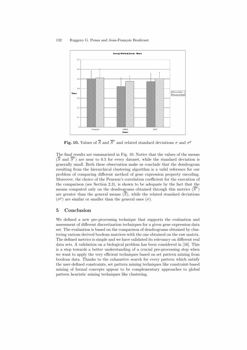
Fig. 10. Values of S and Sp
and related standard deviations σ and σp
The final results are summarized in Fig. 10. Notice that the values of the means(S and S
p) are near to 0.5 for every dataset, while the standard deviation is
generally small. Both these observation make us conclude that the dendrogramresulting from the hierarchical clustering algorithm is a valid reference for ourproblem of comparing different method of gene expression property encoding.Moreover, the choice of the Pearson’s correlation coefficient for the execution ofthe comparison (see Section 2.3), is shown to be adequate by the fact that themeans computed only on the dendrograms obtained through this metrics (S
p)
are greater than the general means (S), while the related standard deviations(σp) are similar or smaller than the general ones (σ).
5 Conclusion
We defined a new pre-processing technique that supports the evaluation andassessment of different discretization techniques for a given gene expression dataset. The evaluation is based on the comparison of dendrograms obtained by clus-tering various derived boolean matrices with the one obtained on the raw matrix.The defined metrics is simple and we have validated its relevancy on different realdata sets. A validation on a biological problem has been considered in [16]. Thisis a step towards a better understanding of a crucial pre-processing step whenwe want to apply the very efficient techniques based on set pattern mining fromboolean data. Thanks to the exhaustive search for every pattern which satisfythe user-defined constraints, set pattern mining techniques like constraint-basedmining of formal concepts appear to be complementary approaches to globalpattern heuristic mining techniques like clustering.
Boolean Property Encoding for Local Set Pattern Discovery 133
Acknowledgements. The authors want to thank Celine Robardet, Sylvain Bla-chon and Olivier Gandrillon for the pre-processing of the SAGE data set, andSophie Rome for her participation to microarray data preparation. Furthermore,we thank Claire Leschi and Jeremy Besson for their contribution to a prelim-inary version of this paper. Finally, this research is partially funded by ACIMD 46 (CNRS STIC 2004-2007) Bingo (Bases de Donnees Inductives pour laGenomique).
References
1. DeRisi, J., Iyer, V., Brown, P.: Exploring the metabolic and genetic control of geneexpression on a genomic scale. Science 278 (1997) 680–686
2. Velculescu, V., Zhang, L., Vogelstein, B., Kinzler, K.: Serial analysis of gene ex-pression. Science 270 (1995) 484–487
3. Piatetsky-Shapiro, G., Tamayo, P., eds.: Special issue on microrray data mining.SIGKDD Explorations, Volume 5, Issue 2 (2003)
4. Eisen, M., Spellman, P., Brown, P., Botstein, D.: Cluster analysis and display ofgenome-wide expression patterns. Proc. Natl. Acad. Sci. USA 95 (1998) 14863–14868
5. Niehrs, C., Pollet, N.: Synexpression groups in eukaryotes. Nature 402 (1999)483–487
6. Boulicaut, J.F., Bykowski, A.: Frequent closures as a concise representation forbinary data mining. In: Proceedings PAKDD’00. Volume 1805 of LNAI., Kyoto,JP, Springer-Verlag (2000) 62–73
7. Pei, J., Han, J., Mao, R.: CLOSET an efficient algorithm for mining frequentclosed itemsets. In: Proceedings ACM SIGMOD Workshop DMKD’00, Dallas,USA (2000) 21–30
8. Zaki, M.J., Hsiao, C.J.: CHARM: An efficient algorithm for closed itemset mining.In: Proccedings SIAM DM’02, Arlington, USA (2002)
9. Becquet, C., Blachon, S., Jeudy, B., Boulicaut, J.F., Gandrillon, O.: Strong-association-rule mining for large-scale gene-expression data analysis: a case studyon human sage data. Genome Biology 12 (2002)
10. Creighton, C., Hanash, S.: Mining gene expression databases for association rules.Bioinformatics 19 (2003) 79 – 86
11. Wille, R.: Restructuring lattice theory: an approach based on hierarchies of con-cepts. In Rival, I., ed.: Ordered sets. Reidel (1982) 445–470
12. Rioult, F., Boulicaut, J.F., Cremilleux, B., Besson, J.: Using transposition forpattern discovery from microarray data. In: Proceedings ACM SIGMOD WorkshopDMKD’03, San Diego (USA) (2003) 73–79
13. Rioult, F., Robardet, C., Blachon, S., Cremilleux, B., Gandrillon, O., Boulicaut,J.F.: Mining concepts from large sage gene expression matrices. In: ProceedingsKDID’03 co-located with ECML-PKDD 2003, Catvat-Dubrovnik (Croatia) (2003)107–118
14. Besson, J., Robardet, C., Boulicaut, J.F.: Constraint-based mining of formal con-cepts in transactional data. In: Proceedings PAKDD’04. Volume 3056 of LNAI.,Sydney (Australia), Springer-Verlag (2004) 615–624
15. Besson, J., Robardet, C., Boulicaut, J.F., Rome, S.: Constraint-based conceptmining and its application to microarray data analysis. Intelligent Data Analysisjournal 9 (2004) To appear.
134 Ruggero G. Pensa and Jean-Francois Boulicaut
16. Pensa, R.G., Leschi, C., Besson, J., Boulicaut, J.F.: Assessment of discretizationtechniques for relevant pattern discovery from gene expression data. In: Proceed-ings ACM BIOKDD’04 co-located with SIGKDD’04, Seattle, USA (2004) 24–30
17. Parthasarathy, S.: Efficient progressive sampling for association rules. In: Proceed-ings IEEE ICDM’02, Maebashi City, Japan (2002) 354–361
18. Moore, G.W., Goodman, M., Barnabas, J.: An iterative approach from the stand-point of the additive hypothesis to the dendrogram problem posed by moleculardata sets. Journal of Theoretical Biology 38 (1973) 423–457
19. Robinsons, D.F.: Comparison of labeled trees with valency three. Journal ofCombinatorial Theory, Series B 11 (1971) 105–119
20. DasGupta, B., He, X., Jiang, T., Li, M., Tromp, J., Zhang, L.: On distancesbetween phylogenetic trees. In: Proceedings ACM-SIAM SODA’97. Volume 55.(1997) 427–436
21. DasGupta, B., He, X., Jiang, T., Li, M., Tromp, J., Zhang, L.: On computing thenearest neighbor interchange distance. In: Discrete mathematical problems withmedical applications (New Brunswick, NJ, 1999), Providence, RI, Amer. Math.Soc. (2000) 125–143
22. Finden, C., Gordon, A.: Obtaining common pruned trees. Journal of Classification2 (1985) 255–276
23. Cole, R., Hariharan, R.: An o(n log n) algorithm for the maximum agreementsubtree problem for binary trees. In: Proceedings of the 7th annual ACM-SIAMsymposium on Discrete algorithms, Atlanta, Georgia, United States (1996) 323–332
24. Bozdech, Z., Llinas, M., Pulliam, B.L., Wong, E., Zhu, J., DeRisi, J.: The tran-scriptome of the intraerythrocytic developmental cycle of plasmodium falciparum.PLoS Biology 1 (2003) 1–16
25. Arbeitman, M., Furlong, E., Imam, F., Johnson, E., Null, B., Baker, B., Krasnow,M., Scott, M., Davis, R., White, K.: Gene expression during the life cycle ofdrosophila melanogaster. Science 297 (2002) 2270–2275
26. Lash, A., Tolstoshev, C., Wagner, L., Schuler, G., Strausberg, R., Riggins, G.,Altschul, S.: SAGEmap: A public gene expression resource. Genome Research 10(2000) 1051–1060