boolean operations of 2-manifolds through vertex …virtual/sgi/articles/mantyla_obs.pdf · boolean...

Boolean Operations of 2-Manifolds through Vertex Neighborhood Classification MARTTI MiiNTY ti Helsinki University of Technology

A topologically complete set operations algorithm for planar polyhedral Z-manifold objects is described; that is, under the assumption that all numerical tests required can be correctly evaluated, the algorithm is capable of solving all “special cases.”

The central component of the algorithm is a module here called the uertex neighborhood classifier. By virtue of the classifier, the various special cases can be reduced into a collection of classification problems involving a pair of coincident vertices. The classifier works by means of decision rules that guarantee the topological consistency and regularity of the resulting polyhedron. If the result is not a 2-manifold, a relaxed polyhedron will be produced.

Categories and Subject Descriptors: 1.3.5 [Computer Graphics]: Computational Geometry and Object Modeling-geometric algorithms, languages, and systems; J.6 [Computer Applications]: Computer-Aided Engineering-computer aided design (CAD)

General Terms: Algorithms

Additional Key Words and Phrases: Boolean operations, set operations, shape operations, solid modeling

-

1. INTRODUCTION

A Boolean set operations algorithm that can be used to unite, intersect, or subtract solid objects with each other is an essential component of any solid modeling system. For human users, set operations offer a tool for describing complex objects in terms of a series of operations on simpler components. For various algorithms, set operations offer a tool for describing physical processes applied to objects. For instance, an algorithm for verifying code for numerically controlled (NC) machine tools can use set operations to model effects of individ- ual machining operations or to determine collisions between the tool and the fixtures [21].

This research has been supported by the Technical Development Center of Finland (TEKES), the Finnish Academy, and the Helsinki University of Technology Foundation. It was partially conducted while the author was visiting Stanford University with the support of the Rotary International Foundation, the Helsinki University of Technology, the Finnish Academy, and the Fund for Finnish Culture. Author’s address: Helsinki University of Technology, Institute of Computing Technology, Laboratory of Information Processing Science, Otakaari 1, SF-02150, Espoo 15, Finland. Permission to copy without fee all or part of this material is granted provided that the copies are not made or distributed for direct commercial advantage, the ACM copyright notice and the title of the publication and its date appear, and notice is given that copying is by permission of the Association for Computing Machinery. To copy otherwise, or to republish, requires a fee and/or specific permission. 0 1986 ACM 0730-0301/86/0100-0001 $00.75

ACM Transactions on Graphics, Vol. 5, No. 1, January 1986, Pages l-29.

2 - Martti Mantyki

A set operations algorithm depends completely on the solid representation used in the modeler. In systems based on the constructive solid geometry (CSG) approach [13, 141, set operations are performed by so-called boundary evaluation 1161, ordinarily based on a “divide-and-conquer” procedure working on a CSG tree that records the description of an object in terms of a collection of solid primitives and several set operations. This family of set operations algorithms is relatively well understood, and its usefulness for the tasks mentioned above has been demonstrated (e.g., [6]).

Systems that use the boundary representation (BR) approach [4] usually include a binary set operations algorithm that works on two boundary models of solids at a time and creates a third boundary model as its result. Requicha and Voelcker [16] use the term boundary merging for this process. These algorithms generally work by comparing, for example, faces of the two solids against each other, and form the desired result by removing the unnecessary parts of the bounding surfaces of the solids. Some CSG systems (e.g., [3]) include a similar procedure for the so-called incremental boundary evaluation [16] that updates a previously evaluated boundary representation when a CSG tree is modified.

Unfortunately, Boolean set operations algorithms for boundary representations are much less well understood than their counterparts for CSG representations. This is so because BR algorithms are plagued by two kinds of problems. First, to be effective, a set operations algorithm must be able to treat all possible kinds of geometric intersections that may appear between faces, edges, and vertices of the two objects. The proper treatment of all cases easily leads to a very hairy case analysis. Second, the very case analysis must be based on various tests for overlap, coplanarity, and intersection, which are difficult to implement robustly in the presence of numerical errors. Perhaps as a result of this complexity, all published descriptions of Boolean set operations algorithms known to the author [2, 5, 7-9, 18, 19, 221 are incomplete in that details on the treatment of special cases are omitted or only partially explained.*

To appreciate the difficulty of the set operations, consider Figure 1, which depicts the set intersection of two extruded profiles. In the figure, the two top views depict two orthogonal profiles. The solid shown in the bottom right view is generated by %weeping” the profiles appropriately to generate overlapping solids and calculating their Boolean intersection. Clearly, the swept objects intersect each other in various “special” ways. In this case a set operations algorithm will have difficulties if it is not prepared to deal with, for example, coplanar overlapping faces such as the bottom face of the resulting object.

Observe that the code of overlapping coplanar faces must be able to handle robustly a two-dimensional set operation of two polygons, a task that even alone is quite challenging for a programmer uninitiated in geometry. All the program code required to break the problem into solvable cases and the codes for each case sum up to a voluminous and complicated algorithm whose correctness is difficult to establish.

This article presents a different path to complete set operations. The algorithm to be presented breaks the Boolean set operations problem into a set of simpler problems of just two major kinds that can be handled with a relatively

’ I apologize for potential misjudgments of cited works.

ACM Transactions on Graphics, Vol. 5, No. 1, January 1986.

e-Manifold Booleans through Vertex Neighborhood Classification l 3

Fig. 1. Set operation of two extruded profiles.

straightforward case analysis. As will be elaborated upon in subsequent sections, the main underlying task involves the processing of two coincident vertices of the two solids, a task termed here the vertex neighborhood classification.

The article is organized as follows: First, the problem statement is elaborated upon, and some terminology introduced in Section 2. Section 3 introduces the basic ideas of the vertex neighborhood classification in the context of the splitting problem, a much simpler relative to the Boolean operations problem. A general- ization of the splitting problem, the boundary classification, and its use in the Boolean operations are discussed in Section 4. Section 5 then outlines the flow of the resulting set operations algorithm.

On the basis of the preceding sections, the vertex neighborhood classifier for Boolean set operations is derived in Section 6. Section 7 gives some practical insights on the numerical problems of the algorithm gained from its experimental implementation. Finally, Section 8 summarizes the results of this work and indicates areas where further research will be needed.

2. STATEMENT OF THE PROBLEM

The algorithms to be discussed work on boundary representations of planar polyhedra. More rigorously, we assume that our objects are 2-manifolds; that is,


4 l Martti M&ttyla

they satisfy the following criteria:

(1) Every edge belongs to exactly two flat faces. (2) Every vertex is surrounded by a single cycle of edges and faces. (3) Faces may not intersect each other except at common edges or vertices.

See [lo] and [15] for further discussion on 2-manifold models. We assume that the polyhedra are represented in terms of a winged-edge data

structure [l] or some equivalent variation of it. That is, we assume the existence of data structures for faces, edges, and vertices and adequate (explicit or implicit) access paths between adjacent entities. Faces may have holes; that is, each face has one “external” bounding loop of edges and zero or more “internal” bounding loops. As typical for the winged-edge data structure, “dangling” edges belonging twice to a face are allowed and are freely used during intermediate stepsof the algorithm.

The polyhedra are assumed to be consistently oriented; that is, the edges around each face must occur in a consistent direction (say, counterclockwise) as viewed from outside the polyhedron. Under this assumption, all face normal vectors point consistently to the outside.

Given two such objects A and 23, our aim is to devise an algorithm that can calculate a new object C that represents the desired regularized [13] Boolean combination of A and B, that is, A U* B, A ‘* B, or A \* B, where U*, A*, and \* are the regularized counterparts of the ordinary (point) set operations union U, intersection *, and set difference \.

Unfortunately, we cannot require that C will always satisfy both of the requirements (1) and (3) above. This is so because 2-manifolds are not closed under set operations; that is, Boolean combination of two 2-manifolds is not necessarily a 2-manifold. For instance, the set difference of the block and the wedge of Figure 2 has four faces meeting at an edge, and criterion (1) is not satisfied.

We accept this limitation because a winged-edge data structure cannot represent objects such as the result of Figure 2 directly. The only resort available is to represent the nonmanifold as a “pseudomanifold”, that is, as if it were one or the other of the objects depicted in Figure 3. In particular, Figure 3a treats the situation as if the wedge extended outside the top face of the block, whereas Figure 3b handles the wedge as if it only intersected the front and the back faces of the block. In Figure 3a, the object has two entirely coincident edges, whereas Figure 3b has an edge lying on a face.

Hence we require that the result of the set operations algorithm satisfy all other criteria except (3). Instead of (3), a more permissive criterion is required:

(3’) Faces of the polyhedron may not intersect each other at their internal points. The only other kinds of intersections are the following:

-Some edges of the polyhedron are entirely coincident. In this case, the edge neighborhoods of these edges must be distinct.

-Some edges may lie on a face. In this case, both faces adjacent to the edge must lie on the same side of the face.

-Some vertices may lie on a face. In this case, all edges and faces adjacent to the vertex must lie on the same side of the face.


2-Manifold Booleans through Vertex Neighborhood Classification l 5

(4 (b)

Fig. 2. Set operations are not closed for 2-manifolds.

(4 (b)

Fig. 3. Pseudomanifold representations of a nonmanifold.

-Some vertices may lie on an edge or on a vertex. In these cases, all edges and faces adjacent to the vertex must lie on the same side of the surface defined by the faces of the incident edge or vertex.

That is, the surface of the resulting object may “touch” itself at some edges or vertices, but not intersect itself properly.


6 l Martti Mfmtylz3

3. DIVERSION: THE SPLITTING PROBLEM

A problem related to Boolean operations is the splitting of a solid with a plane. While being a useful solid modeling tool in its own right, a splitting algorithm forms a good introduction to the much more complicated Boolean operations. Let us, therefore, introduce the basic ideas of the Boolean set operations algorithm in the context of the splitting problem in an intuitive fashion.

A splitting algorithm is expected to divide a polyhedral solid S in two sets determined by the intersection polygons of a splitting plane SP and S. As SP can be conveniently represented in terms of its plane equation

(a b c d) * (x y 2 1) = 0, (1)

we shall call the resulting parts Above and Below, denoting the parts of S in the half-spaces

and

(a b c d) . (x y z 1) P 0 (2)

(a b c d) . (x y z 1) 5 0, (3)

respectively. Of course, we require that Above and Below be in all respects well- formed solids; in particular, if S is regular, Above and Below must be also.

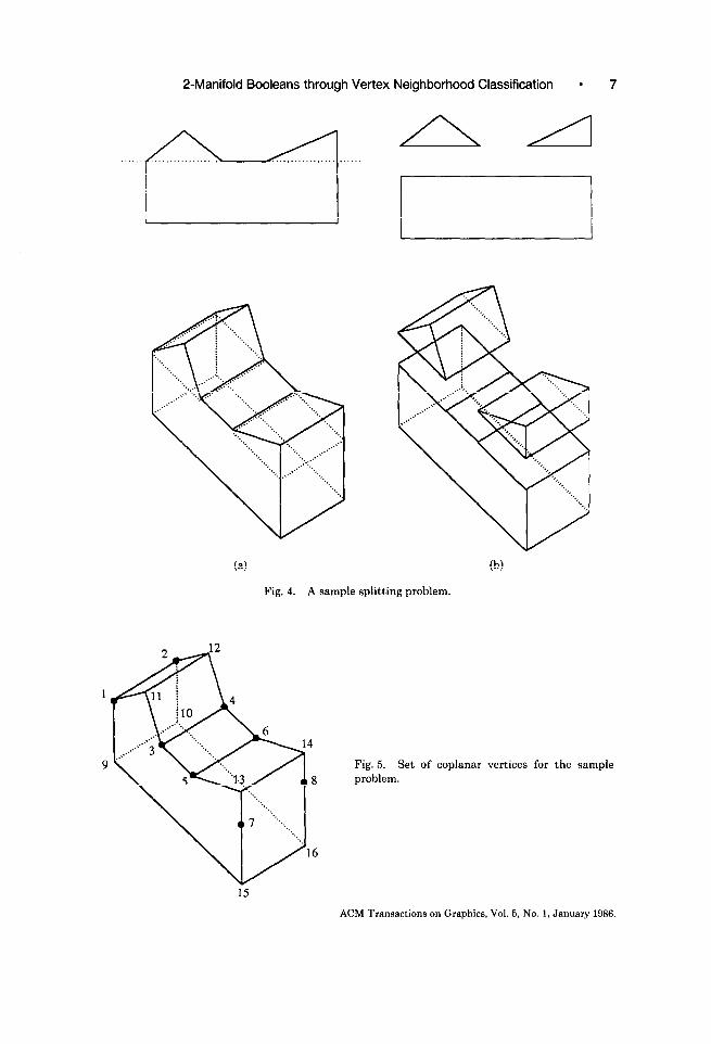
Let us outline the computation of Above and Below intuitively in terms of the sample case depicted in two views in Figure 4. In Figure 4a, the intersection polygon is shown in dashed lines; Figure 4b shows the expected result. Observe that the part Above in this case is a disconnected solid, which is a perfectly acceptable result of the algorithm. (That the top of part Below consists of three coplanar faces is an artifact of the algorithm to be discussed.)

The initial steps of the splitting algorithm considered here are the following:

(1) Locate all edges E of S that intersect SP properly, that is, whose end points are strictly on different sides of SP.

(2) Subdivide each edge found in step (1) at its intersection point with SP. Hence all such edges are replaced by two new edges and a new vertex.

(3) Locate all vertices V of S that lie on SP and store them for later steps. (Of course, the resulting set includes at least all vertices inserted in step (2)) If the set is empty, S and SP do not intersect, and we are done.

After these steps, the splitting problem is effectively reduced into a collection of simpler problems, namely, that of dealing properly with each vertex found in step (3). This computation must be designed so as to guarantee the overall correctness of the result.

Returning to the example of Figure 4, Figure 5 indicates the set of coplanar vertices computed in step (3) above. For reference, these vertices are labeled as 1-8. Labels 9-16 denote the other vertices of S.

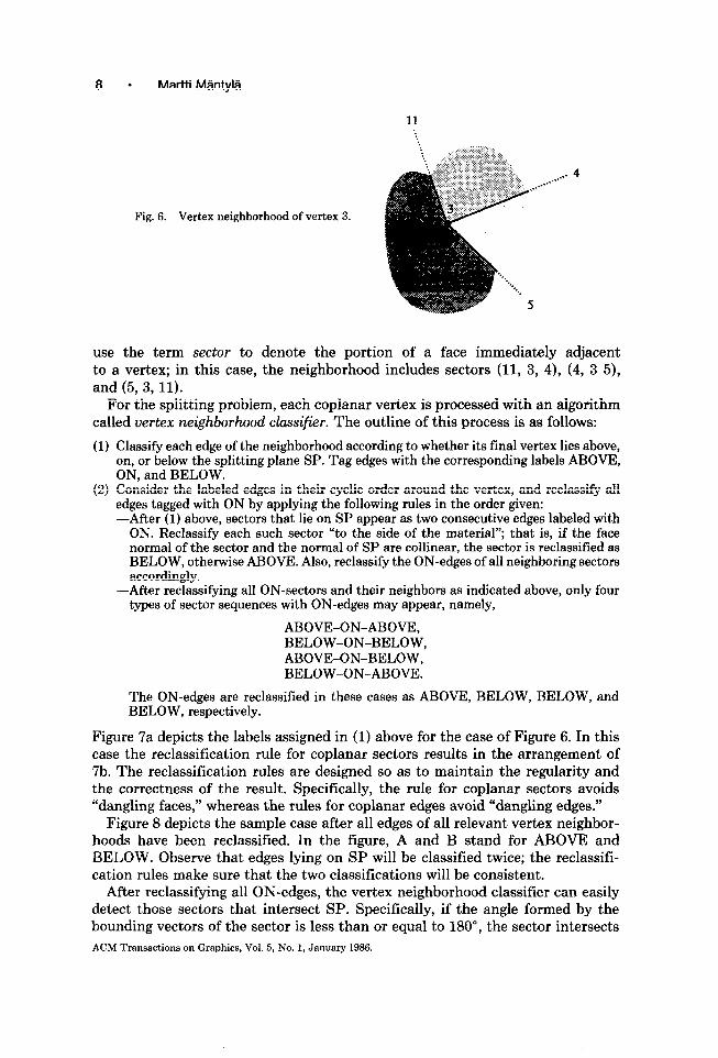
Let us introduce the term vertex neighborhood to denote the ordered cycle of edges and (parts of) faces around a vertex. For instance, the vertex neighborhood of vertex 3 is depicted in Figure 6. This neighborhood consists of the edges (3, ll), (3, 4), and (3, 5); vertices 11, 4, and 5 are termed the final vertices of the edges of the neighborhood; vertex 3 is the base vertex of the neighborhood. We



(4 (b)

Fig. 4. A sample splitting problem.

Fig. 5. Set of coplanar vertices for the sample problem.


8 l Martti MFmtyla

11

;,, .:. . .

. . 4

Fig. 6. Vertex neighborhood of vertex 3.

use the term sector to denote the portion of a face immediately adjacent to a vertex; in this case, the neighborhood includes sectors (11, 3, 4), (4, 3 5), and (5, 3, 11).

For the splitting problem, each coplanar vertex is processed with an algorithm called uertex neighborhood classifier. The outline of this process is as follows:

(1) Classify each edge of the neighborhood according to whether its final vertex lies above, on, or below the splitting plane SP. Tag edges with the corresponding labels ABOVE, ON, and BELOW.

(2) Consider the labeled edges in their cyclic order around the vertex, and reclassify all edges tagged with ON by applying the following rules in the order given: -After (1) above, sectors that lie on SP appear as two consecutive edges labeled with

ON. Reclassify each such sector “to the side of the material”; that is, if the face normal of the sector and the normal of SP are collinear, the sector is reclassified as BELOW, otherwise ABOVE. Also, reclassify the ON-edges of all neighboring sectors accordingly.

-After reclassifying all ON-sectors and their neighbors as indicated above, only four types of sector sequences with ON-edges may appear, namely,

ABOVE-ON-ABOVE, BELOW-ON-BELOW, ABOVE-ON-BELOW, BELOW-ON-ABOVE.

The ON-edges are reclassified in these cases as ABOVE, BELOW, BELOW, and BELOW, respectively.

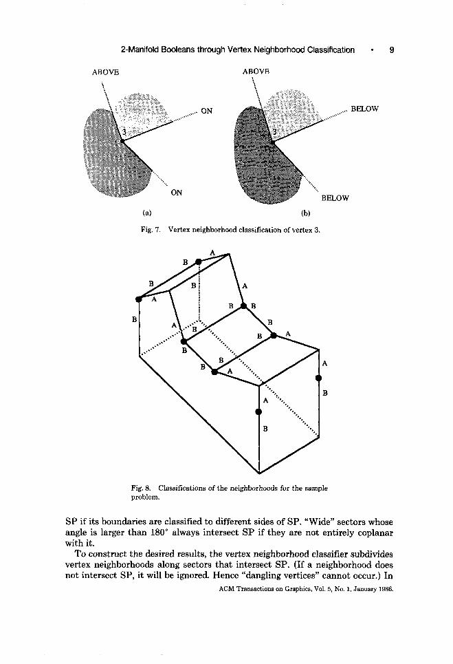
Figure 7a depicts the labels assigned in (1) above for the case of Figure 6. In this case the reclassification rule for coplanar sectors results in the arrangement of 7b. The reclassification rules are designed so as to maintain the regularity and the correctness of the result. Specifically, the rule for coplanar sectors avoids “dangling faces,” whereas the rules for coplanar edges avoid “dangling edges.”

Figure 8 depicts the sample case after all edges of all relevant vertex neighborhoods have been reclassified. In the figure, A and B stand for ABOVE and BELOW. Observe that edges lying on SP will be classified twice; the reclassification rules make sure that the two classifications will be consistent.

After reclassifying all ON-edges, the vertex neighborhood classifier can easily detect those sectors that intersect SP. Specifically, if the angle formed by the bounding vectors of the sector is less than or equal to MO”, the sector intersects ACM Transactions on Graphics, Vol. 5, No. 1, January 1986.


ABOVE ABOVE

: ,....- ON

(4 (b)

Fig. 7. Vertex neighborhood classification of vertex 3.

Fig. 8. Classifications of the neighborhoods for the sample problem.

SP if its boundaries are classified to different sides of SP. “Wide” sectors whose angle is larger than 180” always intersect SP if they are not entirely coplanar with it.

To construct the desired results, the vertex neighborhood classifier subdivides vertex neighborhoods along sectors that intersect SP. (If a neighborhood does not intersect SP, it will be ignored. Hence “dangling vertices” cannot occur.) In


10 l Martti Mfmtylti

ABOVE

Fig. 9. Result of vertex neighborhood classification.

BELOW

null edge

Fig. 10. Computation of the result.

our implementation, the subdivision is accomplished by inserting into the original neighborhood new vertices that share the location of the original vertex. Edges of zero length (null edge) join such new vertices with old ones. Figure 9 depicts this for the case of Figures 6 and 7. Here just one null edge is required.

After applying the classification to all vertices, the final result can be computed by combining the vertices of null edges with new edges in the proper order and removing all null edges. Figure 10 depicts this process, the details of which are unimportant for the current discussion. See [9] and [ll] for additional information.

Observe that the vertex neighborhood classifier for the splitting problem actually solves a particular case of the general set membership classification (SMC) problem [20]. As elaborated by Requicha and Voelcker 1161, SMC is an important tool for boundary evaluation procedures. This suggests that vertex neighborhood classification can play a role in Boolean set operations as well. ACM Transactions on Graphics, Vol. 5, No. 1, January 1986.


4. BOUNDARY CLASSIFICATION

The splitting algorithm outlined in the preceding section is based on reducing the global problem into a collection of local vertex neighborhood classification problems. The classifier works by dividing each vertex neighborhood according to rules that guarantee the correctness of the result. The set operations algorithm and its classifier will follow this general approach.

To see the close relationship between the splitting problem and set operations, recall that the splitting algorithm divides a solid S into two sets (Above, Below) according to a splitting plane SP. For set operations we need the more general splitting of a polyhedron A according to a reference polyhedron B. More rigorously, let us denote the bounding surface of A by b(A). Then the two objects resulting from the general splitting operation will be denoted by AinB (for the part of b(A) inside B) and AoutB (for the part of b(A) outside B).’

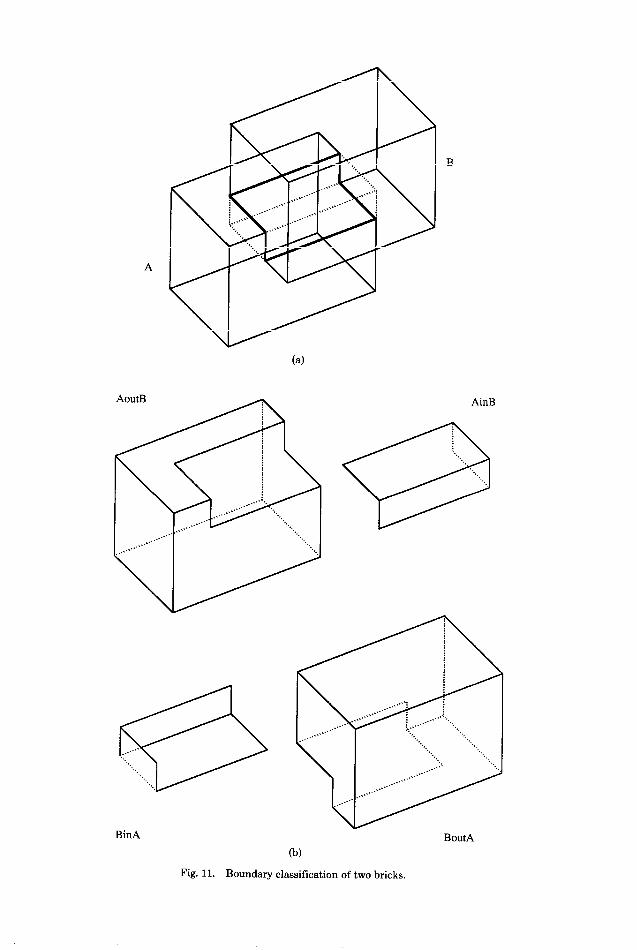
Given two polyhedra A and B, the collection of four objects AinB, AoutB, BinA, and BoutA formed by splitting A against B and symmetrically B against A are here called the boundary classification of A and B. For instance, Figure lla depicts two intersecting bricks; their intersection curve is indicated with heavy lines. The resulting boundary classification is shown in Figure llb. (In the winged-edge representation, each component of the classification is a polyhedron in its own right that generally has some nonplanar “intersection” faces.)

From the boundary classification of A and B, all their Boolean combinations are readily computed:

b(A u B) = AoutB & BoutA,

b(A * B) = AinB & BinA,

b(A \ B) = AoutB & (BinA)-‘,

(4)

where & denotes the “gluing” of two surfaces along a common boundary (in this case, an intersection face), and (BinA)-’ denotes the complement of BinA, that is, BinA with the orientation of all faces reversed. Gluing and complementation can be implemented relatively easily for boundary representations (e.g., [2]), and we do not elaborate upon these procedures.

In the splitting algorithm, the vertex neighborhood classifier treats edges and faces lying on the splitting plane by reclassifying them as lying above or below the plane. The reclassification rules are designed so as to guarantee the regularity of the result. A similar approach can be followed also in the classifier for set operations. In this case, however, the reclassification rules will be more complicated.

To provide insight into the reclassification rules, it is useful to consider the eight-way boundary classification of A and B that adds the components AonB+, AonB-, BonA+, and BonA- to the components of the four-way classification (AinB, AoutB, BinA, BoutA). AonB+ consists of those parts of b(A) that lie on b(B) so that the face normals of the respective faces are equal, whereas AonB-

’ Observe that this is exactly what the splitting algorithm does if we think of the halfspace “above” SP as a polyhedron B bounded by just one infinite face.


AoutB

53 . . ...‘. . .._ ‘.._ ‘...

BinA

AinB

BoutA

(b)

Fig. 11. Boundary classification of two bricks.


Table I. Reclassification Rules for ON-Components

Set operation AonB+ AonB- BonA+ BonA- U AoutB AinB BinA BinA A

AinB AoutB Bout4 BoutA \ AoutB AinB Bout.4 BoutA

consists of the overlapping parts where the normals are opposite. BonA+ and Bowl- are defined analogously.

Figure 12 illustrates the eight-way boundary classification of two objects A and B shown in three views. For clarity, the IN- and ON-components of the classification are shaded.

From the components of the eight-way classification, the result of a set operation can be computed as follows:

b(A U B) = AoutB & BoutA & AonB+,

b(A A B) = AinB & BinA & AonB+, (5)

b(A \ B) = AoutB & (BinA)-’ & AonB-.

(The reader is encouraged to check that these equations indeed give the correct regularized results for the objects of Figure 12.)

It would be perfectly possible to construct a set operations algorithm that computes the full eight-way boundary classification, and works out the result according to eqs. (4). Because of the inherent burden of this computation, we do not follow this approach directly. Instead, our algorithm calculates a four-way boundary classification in which the ON-components of the eight-way classification are lumped with the components of the four-way classification so as to make eqs. (4) and (5) equivalent.

A set of reclassification rules with this property is shown in Table I. It should be stressed that these rules will be implemented directly in the vertex neighborhood classifier, and that higher levels of the algorithm can effectively ignore all ON-cases. (Observe the analogy of the rules of Table I and the reclassification of ON-edges in the splitting algorithm of Section 3.)

5. OUTLINE OF THE BOOLEAN .SET OPERATIONS ALGORITHM

We can now formulate the initial steps of the algorithm as follows:

(1)

(2)

(3) (4)

(5)

(6)

Locate all pairs of edges EA of A and Es of B that intersect each other properly, that is, at an internal point of both edges. Subdivide both edges at their intersection point, that is, replace each edge by two edges and a new vertex lying at the intersection point. Locate all edges of A that pass through a vertex of B. Subdivide all such edges at the intersection point. Do step (2) symmetrically for edges of B and vertices of A. Locate all coincident pairs of vertices Va of A and VB, and store them for later processing. (Of course, the resulting set includes at least all vertices added during steps (l)-(3).) Locate all edges EA of A that intersect a face Fs of B properly, that is, at an internal point of F. Subdivide all such edges at the intersection point. Do step (5) symmetrically for edges of B and faces of A.


16 l Martti Mtintyki

(7) Locate all vertices VA of A that lie within a face FB of B and store the pair (VA, Fs) for later processing. (This set will include all vertices added during step (5))

(8) Locate all vertices Ve of B that lie within a face FA of A and store the pair ( Vg, FA) for later processing. (This set includes all vertices added in step (6).)

(The reader is urged to compare these steps with those of the splitting algorithm in Section 3. In particular, note the analogy of steps (5)-(8) of this algorithm with the splitting algorithm.)

After these steps, the problem is reduced into a collection of problems of two kinds:

-dealing with a vertex of one solid that lies on a face of the other solid, -dealing with a pair of coincident vertices of A and B.

Both of these problems are solved by a vertex neighborhood classifier that inserts the proper null edges as to split the vertex neighborhoods into subcycles inside and outside of the respective other polyhedron. The components of the four-way classification are then constructed just as in the case of the splitting algorithm, and the final polyhedron is computed according to eqs. (4). We do not elaborate these parts of the algorithm.

6. VERTEX NEIGHBORHOOD CLASSIFICATION

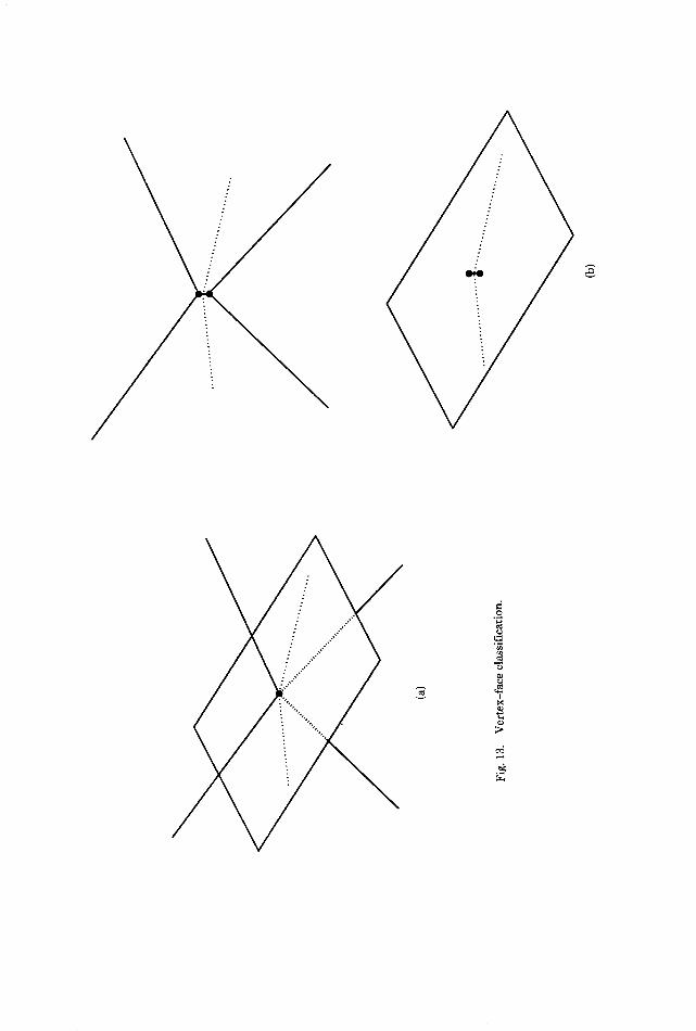
As discussed in the preceding section, the vertex neighborhood classification is required in the set operations algorithm in two forms:

(1) Vertex-face classification: The classification of a vertex neighborhood with respect to a face. By construction, the vertex is known to be coplanar and properly within the face.

(2) Vertex-uertex classification: The classification of two vertex neighborhoods with respect to each other. By construction, the vertices are coincident.

The following subsections elaborate these tasks.

6.1 Vertex-Face Classification

For the vertex-face classification, a classifier essentially identical as that of the splitting problem can be used. The differences between this case and the splitting problem are the following:

-Instead of the splitting plane SP, the plane of the face is used, and the notions of “above” and “below” are replaced by “in” and “out” (recall that face normals point consistently out from the solid).

-ON-sectors are reclassified according to Table I instead of the rule stated in Section 2.

--In addition to splitting the vertex neighborhood, a reference of the intersection point must also be stored within the face so that the intersection polygon(s) can be drawn through the point.

As for the last item, our algorithm for combining null edges can work properly if the intersections are marked by inserting a null edge as an internal loop into the face intersected; see Figure 13. (Such “dangling” edges are structurally allowed in the winged-edge data structure; they will be removed in the final phases of the algorithm.) ACM Transactions on Graphics, Vol. 5, No. 1, January 1986.

18 l Martti Mhtyh

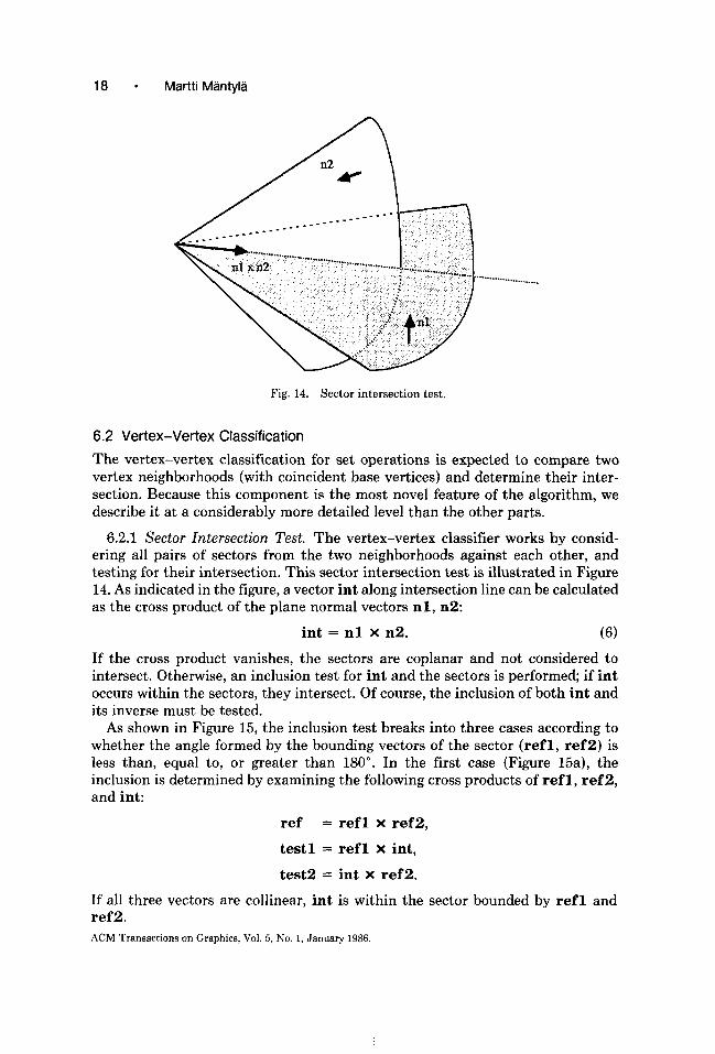
Fig. 14. Sector intersection test,

6.2 Vertex-Vertex Classification

The vertex-vertex classification for set operations is expected to compare two vertex neighborhoods (with coincident base vertices) and determine their intersection. Because this component is the most novel feature of the algorithm, we describe it at a considerably more detailed level than the other parts.

6.2.1 Sector Intersection Test. The vertex-vertex classifier works by consid- ering all pairs of sectors from the two neighborhoods against each other, and testing for their intersection. This sector intersection test is illustrated in Figure 14. As indicated in the figure, a vector int along intersection line can be calculated as the cross product of the plane normal vectors nl, n2:

int = nl X n2. (6)

If the cross product vanishes, the sectors are coplanar and not considered to intersect. Otherwise, an inclusion test for int and the sectors is performed; if int occurs within the sectors, they intersect. Of course, the inclusion of both int and its inverse must be tested.

As shown in Figure 15, the inclusion test breaks into three cases according to whether the angle formed by the bounding vectors of the sector (refl, ref2) is less than, equal to, or greater than 180”. In the first case (Figure 15a), the inclusion is determined by examining the following cross products of ref 1, ref 2, and int:

ref = refl X ref2,

test1 = refl X int,

test2 = int X ref2.

If all three vectors are collinear, int is within the sector bounded by refl and ref2. ACM Transactions on Graphics, Vol. 5, No. 1, January 1986.

20 ’ Martti MWtyla

(a) (b)

Fig. 16. Edge-sector coincidence and edge-edge coincidence.

The second case is simply solved by testing the inclusion of int in the complement of the sector and negating the result. In the final case, a fourth vector in that points to the inside of the sector is formed, and the inclusion of int can be determined by examining the sign of the dot product of int and in.

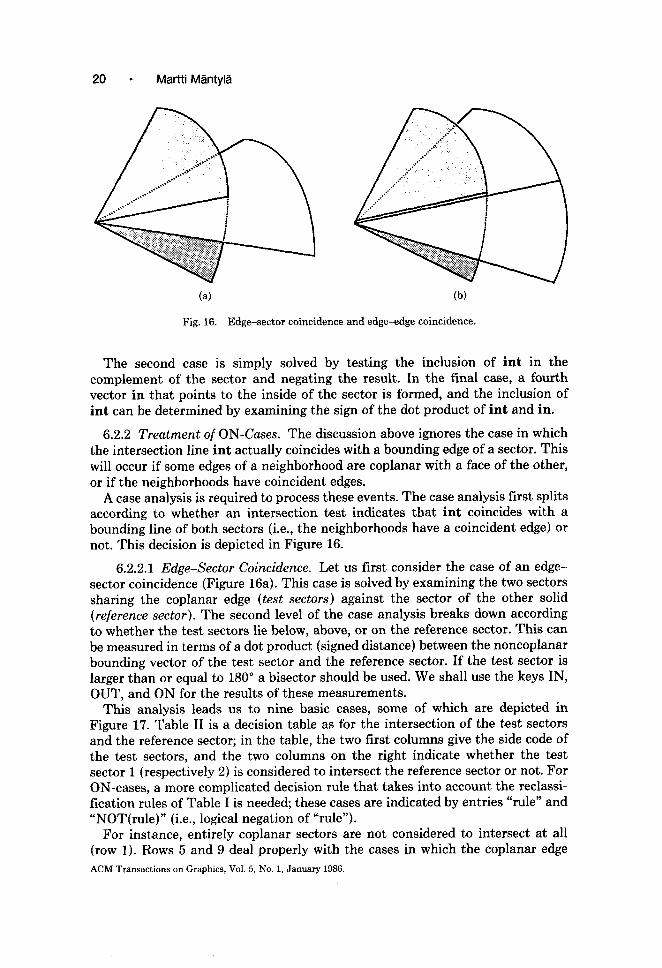
6.2.2 Treatment of ON-Cases. The discussion above ignores the case in which the intersection line int actually coincides with a bounding edge of a sector. This will occur if some edges of a neighborhood are coplanar with a face of the other, or if the neighborhoods have coincident edges.

A case analysis is required to process these events. The case analysis first splits according to whether an intersection test indicates that int coincides with a bounding line of both sectors (i.e., the neighborhoods have a coincident edge) or not. This decision is depicted in Figure 16.

6.2.2.1 Edge-Sector Coincidence. Let us first consider the case of an edge- sector coincidence (Figure 16a). This case is solved by examining the two sectors sharing the coplanar edge (test sectors) against the sector of the other solid (reference sector). The second level of the case analysis breaks down according to whether the test sectors lie below, above, or on the reference sector. This can be measured in terms of a dot product (signed distance) between the noncoplanar bounding vector of the test sector and the reference sector. If the test sector is larger than or equal to 180” a bisector should be used. We shall use the keys IN, OUT, and ON for the results of these measurements.

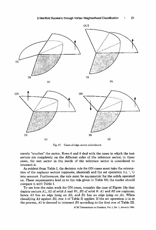
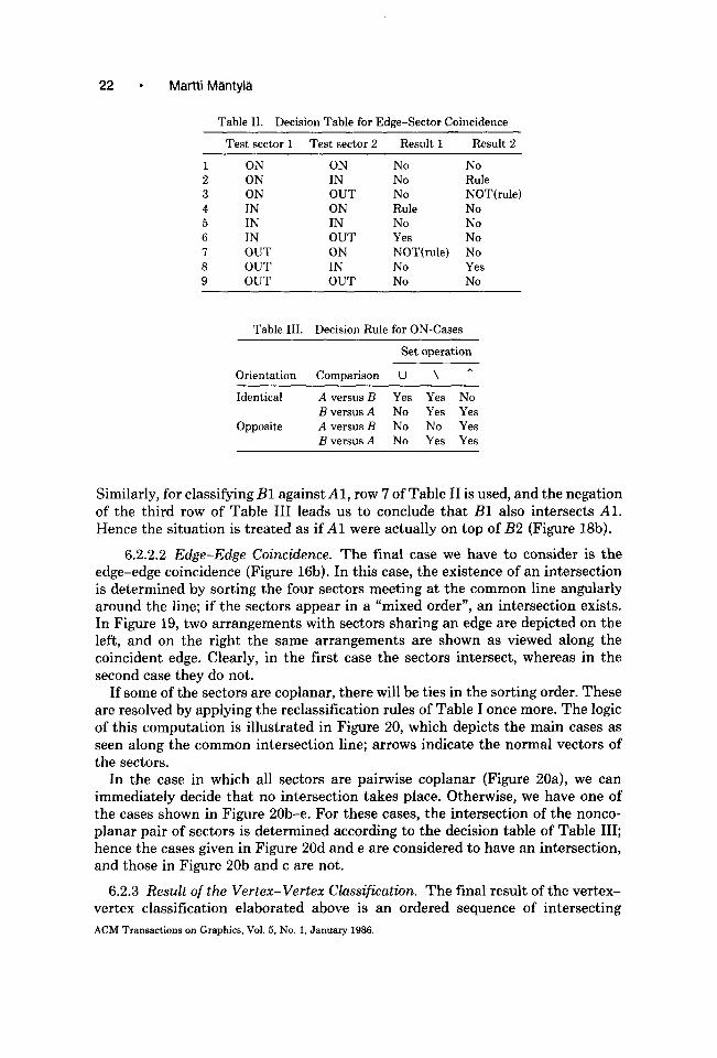
This analysis leads us to nine basic cases, some of which are depicted in Figure 17. Table II is a decision table as for the intersection of the test sectors and the reference sector; in the table, the two first columns give the side code of the test sectors, and the two columns on the right indicate whether the test sector 1 (respectively 2) is considered to intersect the reference sector or not. For ON-cases, a more complicated decision rule that takes into account the reclassification rules of Table I is needed; these cases are indicated by entries “rule” and “NOT(rule)” (i.e., logical negation of “rule”).

For instance, entirely coplanar sectors are not considered to intersect at all (row 1). Rows 5 and 9 deal properly with the cases in which the coplanar edge ACM Transactions on Graphics, Vol. 5, No. 1, January 1986.

2-Manifold Booleans through Vertex Neighborhood Classification

OUT

l 21

(a) (b)

ON ON

IN

(4

Fig. 17. Cases of edge-sector coincidence.

merely “touches” the sector. Rows 6 and 8 deal with the cases in which the test sectors are completely on the different sides of the reference sector; in these cases, the test sector in the inside of the reference sector is considered to intersect it.

As evident from Table I, the decision rule for ON-cases must take the orientation of the coplanar sectors (opposite, identical) and the set operation (U, *, \) into account. Furthermore, the rule must be asymmetric for the solids operated on. These requirements lead us to the rule given in Table III; the reader should compare it with Table I.

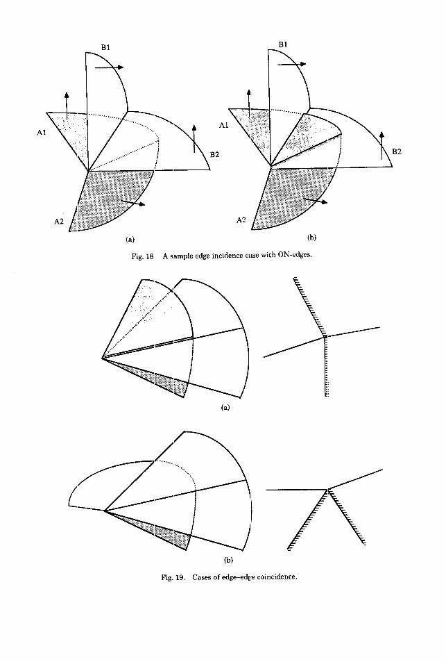
To see how the rules work for ON-cases, consider the case of Figure 18a that depicts sectors Al, A2 of solid A and Bl, B2 of solid B. Al and B2 are coplanar; hence A2 has an edge lying on B2, and Bl has an edge lying on Al. When classifying A2 against B2, row 4 of Table II applies. If the set operation U is in the process, A2 is deemed to intersect B2 according to the first row of Table III.


22 l Martti Mantyh

Table 11. Decision Table for Edge-Sector Coincidence

Test sector 1 Test sector 2 Result 1 Result 2

ON ON ON IN IN IN OUT OUT OUT

ON IN OUT ON IN OUT ON IN OUT

No No No Rule No NOT(rule) Rule No No No Yes No NOT(rule) No No Yes No No

Table III. Decision Rule for ON-Cases

Set operation

Orientation Comparison U \ A

Identical A versus B Yes Yes No B versus A No Yes Yes

Opposite A versus B No No Yes B versus A No Yes Yes

Similarly, for classifying Bl against Al, row 7 of Table II is used, and the negation of the third row of Table III leads us to conclude that Bl also intersects Al. Hence the situation is treated as if Al were actually on top of B2 (Figure 18b).

6.2.2.2 Edge-Edge Coincidence. The final case we have to consider is the edge-edge coincidence (Figure 16b). In this case, the existence of an intersection is determined by sorting the four sectors meeting at the common line angularly around the line; if the sectors appear in a “mixed order”, an intersection exists. In Figure 19, two arrangements with sectors sharing an edge are depicted on the left, and on the right the same arrangements are shown as viewed along the coincident edge. Clearly, in the first case the sectors intersect, whereas in the second case they do not.

If some of the sectors are coplanar, there will be ties in the sorting order. These are resolved by applying the reclassification rules of Table I once more. The logic of this computation is illustrated in Figure 20, which depicts the main cases as seen along the common intersection line; arrows indicate the normal vectors of the sectors.

In the case in which all sectors are pairwise coplanar (Figure 20a), we can immediately decide that no intersection takes place. Otherwise, we have one of the cases shown in Figure 20b-e. For these cases, the intersection of the noncoplanar pair of sectors is determined according to the decision table of Table III; hence the cases given in Figure 20d and e are considered to have an intersection, and those in Figure 20b and c are not.

6.2.3 Result of the Vertex-Vertex Classification. The final result of the vertex- vertex classification elaborated above is an ordered sequence of intersecting ACM Transactions on Graphics, Vol. 5, No. 1, January 1986.

24 l Martti M?mtyh

(4

lb)

(4 (4

Fig. 20. Ties in the angular sort.

sector pairs, as depicted schematically in Figure 21a. In the figure, dashes indicate sector intersection lines; hence sectors (2, 1, 3), (7, 6, 8) and (4, 1, 5), (9, 6, 10) intersect each other.

Clearly, sector intersections indicate locations where the neighborhoods should be subdivided so as to separate the subsequences inside and outside the other sector from each other. Again, our algorithm encodes the subdivision by inserting null edges appropriately (Figure 21b).

Frequently, a sector has several intersections with sectors from the other neighborhood. A typical arrangement is depicted in Figure 22a. This situation can be encoded by using a dangling null edge, as shown in Figure 22b.

7. REMARKS ON NUMERICAL PROBLEMS

As noted in Section 1, numerical accuracy is one of the major problems that the designer of a Boolean set operations algorithm must live with. For fairness, let us discuss some of the practical lessons learned while implementing the algorithm described. A word of warning: The author has not analyzed completely the numerical properties of the algorithm and cannot describe exactly under which assumptions the numerical results will be correct. Hence this section should be understood as an informal introduction into an area well worth a separate article.

As described, the set operations algorithm requires a variety of tests for intersection, coplanarity, and coincidence. More accurately, the reduction phase of the algorithm (steps (l)-(8) of Section 5) requires the following tests:

(1) a test for the intersection of two lines in three-space (step (l)), (2) a test for the coincidence of two points in three-space (step (4)), (3) a test for coplanarity of a point on a plane in three-space (steps (7) and (8)), ACM Transactions on Graphics, Vol. 5, No. 1, January 1986.

e-Manifold Booleans through Vertex Neighborhood Classification l 25

2

‘)

(4

5

(b)

Fig. 21. Result of vertex-vertex classification.

(4) a point-in-polygon test in three-space (steps (7) and (ES)), (5) a test for the intersection of a polygon and a noncoplanar edge in three-space

(steps (5) and (6)).

The vertex neighborhood classifier requires the additional test of collinearity of two vectors of three-space. Currently, this test is implemented by computing the cross product of the (normalized) vectors and examining whether the resulting vector is of zero length.

As such, none of these problems is particularly difficult. In the context of set operations, however, the collection of these routines must be implemented carefully. To see why, observe that faces are hardly ever really planar. Owing to imperfect arithmetic, the points forming the boundary of a face usually have a nonzero distance to the plane of the face.


26 l Martti Mantyki

(a)

(b)

Fig. 22. Another result of vertex-vertex classification.

Even with imperfect data, the geometric tests are expected to produce consistent results. Consider, for instance, the case depicted in Figure 23. In the figure, edge El intersects the object with faces Fl and F2 somewhere “near” edge E2.

In this case, the geometric tests should yield one of the following outcomes:

-The intersection point P is reported to lie within F1, and P does not lie on E2 or within F2.

-P is reported to lie within F2 and outside of E2 and FL -P is reported to lie on E2 and on the boundary of F1 and F2.

If, owing to numerical errors, P were reported, say, to occur within both F1 and F2, the set operations algorithm would fail.

To enforce consistency, the current implementation of our set operations algorithm employs two guidelines. First, the algorithms that implement the geometric tests form a hierarchy in which “high-level” modules use the services of “low-level” ones. For instance, to examine whether a point lies on the boundary of a face, the point-in-polygon procedure uses the point-on-edge procedure and ACM Transactions on Graphics, Vol. 5, No. 1, January 1986.

P-Manifold Booleans through Vertex Neighborhood Classification . 27

Fig. 23. Consistency.

the point coincidence procedure. In turn, the point-on-edge procedure works by projecting the test point on the edge and testing the coincidence of the test point and the projected point. In this fashion all intersection tests are reduced to point coincidence tests. This approach guarantees that identical measures are applied throughout the procedures.

Second, the order in which the various tests are applied and the tolerances for the point coincidence tests needed are selected carefully so as to enforce consistency. For instance, the test for edge-edge intersection is applied before edge-face tests (and with larger tolerances) to avoid wrong results. Naturally, all tolerances are calculated on the basis of the actual dimensions of the objects worked on. (See [17] for an approach of deriving some of the required tolerances.)

In our experience, these measures are not sufficient to enforce the correct treatment of approximately coplanar faces. Therefore our actual implementation handles them separately to make sure that all edge-edge intersections, etc., caused by overlapping coplanar faces are noticed and processed.

8. CONCLUSIONS

We have presented an algorithm for Boolean set operations of 2-manifold polyhedral solids that can solve all special cases that may arise, provided that the required geometric tests can be performed consistently. As for now, we have not been able to analyze rigorously the conditions under which this limiting assumption will be satisfied. If the resulting object is not a 2-manifold, a pseudomanifold object will be computed.

As suggested by Requicha and Voelcker [16], the techniques for classification and neighborhood analysis developed for boundary evaluation of CSG models are applicable to the evaluation of Boolean operations of BR models as well. Indeed, the algorithm described can be regarded as a particular way to implement the


28 l Martti MBntylii

theoretical procedures that Requicha and Voelcker outline in their article. How- ever, whereas they concentrate on explicitly represented face and edge neighborhoods, our algorithm is based on implicitly represented vertex neighborhoods. Moreover, our algorithm is much more economical by exploiting the adjacency information usually available in “data-rich” boundary representations such as the winged-edge representation, and by avoiding point-in-polyhedron tests completely (except for the case that the surfaces of the solids do not intersect at all).

The algorithm does not extend directly to objects with curved faces or to nonmanifold objects. Curved faces may intersect each other in a way that cannot be reduced to vertex-vertex coincidences (consider spheres, for instance). Set operations of nonmanifolds would require the classification of several vertex neighborhoods from one object against several neighborhoods from the other, instead of the one-against-one case handled by this algorithm.

As presented, the algorithm is slow. A careful implementation of steps (l)-(8) of Section 5 can speed it up by a factor of 10 or so, but after these enhancements the search of intersecting entities starts to dominate the computation time. As noted by Requicha and Voelcker [16], however, the worst-case analysis of the computational efficiency for set operations is not very informative as to the practical speed of the algorithm, and advanced geometric search techniques can be applied to it so as to exploit the typical geometric locality of the computation. An example of this has been described in a previous paper [12].

ACKNOWLEDGMENTS

The thorough and helpful comments of the reviewers on preliminary versions of the article are gratefully acknowledged. The comments of Markku Tamminen also helped to clarify the article.

REFERENCES

1. BAUMGART, B. Geometric modeling for computer vision. Ph.D. dissertation, Computer Science Dept., Stanford Univ. Stanford, Calif., 1974. Also as Tech. Rep. CS-463, Computer Science Dept., Stanford Univ.

2. BRAID, I. C. Notes on a geometric modeller. CAD Group Document 101, Computer Laboratory, Univ. of Cambridge, Cambridge, England, June 1979. (Revised 1980.)

3. BROWN, C. M. PADL-2: A technical summary. IEEE Comput. Graph. Appl. 2, 2 (Mar. 1982), 69-84.

4. HILLYARD, R. The BUILD family of solid modelers. ZEEE Comput. Graph. Appl. 2, 2 (Mar. 1982), 43-52.

5. HOSAKA, M., KIMURA, F., AND KAKISHITA, N. A unified method for processing polyhedra. In Information Processing 1974. North-Holland Publ., Amsterdam, 1974.

6. HUNT, W. A. An explanatory study of automatic verification of programs for numerically controlled machine tools. M.S. thesis, Mechanical and Aerospace Sciences Dept., Univ. of Rochester, Rochester, N. Y., 1979.

7. KALAY, Y., AND EASTMAN, C. M. Shape operations, an algorithm for spatial set manipulations of solid objects. Res. Rep, 10, Dept. of Architecture, Carnegie-Mellon Univ., Pittsburgh, Pa., July 1980.

8. LANIJSSE, A. A general algorithm for performing polyhedral set operations. Presentation given in SIAM Conference on Geometric Modeling and Robotics (Albany, N. Y., July 15-19). 1985.

9. MKNTYLK, M. Set operations algorithm of GWB. Comput. Graph. Forum 2, 2/3 (Aug. 1983), 122-134.


2-Manifold Booleans through Vertex Neighborhood Classification . 29

10. M~~NTYL& M. A note on the modeling space of Euler operators. Comput. Vision, Graph. Image Process. 26, 1 (Apr. 1984), 45-60.

11. M&NTYL& M., AND SULONEN, R. GWB: A solid modeler with Euler operators. IEEE Comput. Graph. Appl. 2, 7 (Sept. 1982), 17-31.

12. MANTYLA, M., AND TAMMINEN, M. Localized set operations for solid modeling. Comput. Graph. 17,3 (July 1983), 279-288.

13. REQUICHA, A. A. G. Representation of solid objects: Theory, methods, and systems. ACM Comput. Sura 12,4 (Dec. 1980), 437-464.

14. REQUICHA, A. A. G., AND VOELCKER, H. B. Constructive solid geometry. Tech. Memo. No. 27, Production Automation Project, Univ. of Rochester, Rochester, N. Y., 1977.

15. REQUICHA, A. A. G., AND VOELCKER, H. B. Solid modeling: Current status and research directions. IEEE Comput. Graph. Appl. 3, 7 (Oct. 1983), 25-37.

16. REQUICHA, A. A. G., AND VOELCKER, H. B. Boolean operations in solid modeling: Boundary evaluation and merging algorithms. Proc. IEEE 73, 1 (Jan. 1985), 30-44.

17. SEGAL, M., AND SEQUIN, C. H. Consistent calculations for solids modeling. In Proceedings of the First Conference on Compututional Geometry (Baltimore, Md., June 5-7). ACM, New York, 1985, pp. 29-38.

18. STEINBERG, H. A. Overlap and separation calculations using the SynthaVision three dimensional solid modeling system. In Proceedings of the Conference on CAD/CAM Technology in Mechanical Engineering (Cambridge Mass., March 24-26). 1982, pp. 13-19.

19. STROWEIS, J., AND HANRAHAN, P. Spatial set operations on manifolds. Presentation given in SIAM Conference on Geometric Modeling and Robotics (Albany, N. Y., July 15-19). 1985.

20. TILOVE, R. B. Set membership classification: a unified approach to geometric intersection problems. IEEE Trans. Comput. C-29, 10 (Oct. 1982), 847-883.

21. VOELCKER, H. B., AND REQUICHA, A. A. G. Geometric modeling of physical parts and processes. IEEE Comput. 10,2 (Dec. 1977), 48-57.

22. YAMACUCHI F., AND TOKIEDA, T. A unified algorithm for Boolean shape operations. IEEE Comput. Graph. Appl. 4,6 (June 1984), 24-37.

Received August 1985; accepted June 1986.


boolean operations of 2-manifolds through vertex …virtual/sgi/articles/mantyla_obs.pdf · boolean...

Documents