book review: - lahore school of · web viewbook review: globalization and its discontents qais...
TRANSCRIPT

THE LAHORE JOURNAL
OFECONOMICS
Lahore School of Economics
M. Abdul Mateen KhanPolitical Economy of Fiscal Policy in Pakistan
Imran Ashraf Toor and Muhammad Sabihuddin ButtSocioeconomic and Environment Conditions and Diarrheal Disease Among Children in Pakistan
Umer KhalidOpportunities and Challenges for Pakistan in an Era of Globalisation
Muhammad Aslam Chaudhary and Amjad Naveed Export Earnings, Capital
AurangzebTrade, Investment and Growth Nexus in Pakistan:An Application of Cointegration and Multivariate Causality Test
Asad Sayeed, Farhan Sami Khan and Sohail Javed Income Patterns of Woman Workers in Pakistan –A Case Study of the Urban Manufacturing Sector
Atif NaveedStock Market

Instability and Economic Growth in South Asia
Aamir Ali ChughtaiA Comparative Analysis of Job Satisfaction Among PublicAnd Private Sector College / University Teachers in Lahore
Development and Financial IntermediaryDevelopment in Pakistan(1991-2001)
Book Review:
Qais AslamGlobalization and its Discontents
Volume 8, No.1 Jan-June, 2003

THE LAHORE JOURNALOF
ECONOMICS
Editorial Board
Dr. Shahid Amjad Chaudhry EditorProf. Viqar Ahmed EditorDr. Salman Ahmad EditorMs. Nina Gera Co-Editor
Editorial Advisory BoardDr. Rashid AmjadDr. Pervez TahirDr. Khalid AftabDr. A. R. KemalDr. Moazam MehmoodDr. Naved HamidDr. Tariq Siddiqui
Dr. Munir AhmadDr. Nasim Hasan ShahDr. Sarfraz QureshiDr. Shahrukh Rafi KhanDr. Akmal HusainTariq HusainDr. Aslam ChaudhryDr. Nuzhat Ahmad
Editorial Staff: Tele. No: 5712240Telefax: 0092 - 42 - 5714936E-mail: [email protected]
Publisher : Lahore School of Economics, Lahore, Pakistan.
Correspondence relating to subscriptions and changes of address should be sent to The Lahore Journal of Economics, 105-C-2, Gulberg III, Lahore - 54660 - Pakistan
Instructions to authors can be found at the end of this issue. No responsibility for the views expressed by authors and reviewers in The

Lahore Journal of Economics is assumed by the Editor, the Co-Editor and the Publishers.
Copyright by: Lahore School of Economics
82003


THE LAHORE JOURNAL OF ECONOMICS
Contents Vol. 8, 2003Political Economy of Fiscal Policy in Pakistan
M. Abdul Mateen Khan 1Socioeconomic and Environment Conditions andDiarrheal Disease Among Children in Pakistan
Imran Ashraf Toor and Muhammad Sabihuddin Butt 25
Opportunities and Challenges for Pakistan in anEra of Globalisation
Umer Khalid 45
Export Earnings, Capital Instability and Economic Growth in South Asia
Muhammad Aslam Chaudhary and Amjad Naveed 65A Comparative Analysis of Job Satisfaction Among Public andPrivate Sector College / University Teachers in Lahore
Aamir Ali Chughtai 91
Trade, Investment and Growth Nexus in Pakistan:An Application of Cointegration andMultivariate Causality Test
Aurangzeb 119
Income Patterns of Woman Workers in Pakistan –A Case Study of the Urban Manufacturing Sector
Asad Sayeed, Farhan Sami Khan and Sohail Javed 139
Stock Market Development and Financial IntermediaryDevelopment in Pakistan (1991-2001)
Atif Naveed 155
Book Review:Globalization and its Discontents
Qais Aslam 177

M. Abdul Mateen Khan
Political Economy of Fiscal Policy in Pakistan
M. Abdul Mateen Khan*
1. Introduction
In an underdeveloped country the state regulates not only the short- term performance of the economy but also its path of development. Such an overwhelming role of the state derives its justification from the very nature of underdevelopment itself. Economics and economists are usually concerned with policy. with a view to determining as to what policies are appropriate in a given economic situation to attain policy objectives such as economic growth, full employment, price stability, redistribution of income and wealth. But adopted policies are often not the policies that economists recommend as the best or even the second best.
It is generally observed that vested interests and pressure groups compete for a greater share in the resources and only those policies have to be put into practice in a society which are adopted by all or a significant majority. The basis of decision-making is not economic factors alone and the influence of non-economic factors has been found more important in terms of compromising the interest of transparency as well as the system in almost all developing countries as against the developed countries1. Pakistan is no exception.
The political economy of fiscal policy is generally studied in three stages. (1) Analysis of the economic situation and prescription of policies: (2) The process of decision-making: (3) Implementation of policies: The first stage is the economic one. The second and third stages are more relevant in analysing the problem of policy-* Director. Foreign Service Academy, Islamabad.1 See Schinichi Ichimura, ‘A Conceptual Framework for the Political Economy of Policy Making’ in The Political Economy of Fiscal Economy , Ed. Mignal Urutia, UN University. 1989.
1

The Lahore Journal of Economics, Vol.8, No.1
making and if one is to see (1) who participates in the decision-making and (2) how much freedom is allowed in decision-making. It explains the weaknesses and strength of the given policy.
This paper investigates the political and economic factors that affect decision-making and the implementation of fiscal policies in Pakistan and not the policy itself. After the introduction Part 2 discusses the theoretical framework of the dimension of policy-making. Part 3 illustrates various aspects of fiscal policy making in Pakistan. Subsequently, the measures taken by the military regime, which took over the government in 1999, are discussed as a case study in Part 4. Various sources for the study include Annual Economic Surveys of Pakistan, which provide sufficient data and details of the policies adopted by the government and their effectiveness, research work undertaken in this and the relevant field papers, published articles and comments.
2. Dimensions of Policy Making
Despite the triumph of capitalism and the general acceptance of liberal economic principles, in real society there is no perfect freedom to choose in many decisions. In the present day nation state system, there are many government regulations, and one often needs the government's permission to undertake economic activities2. Ichimura (989) provides a framework with which to analyse decision-making within available environments ranging from one extreme case of control to the other end, that is total freedom.
Fig.-1: Dimensions ofPoIitica1 Aspects of Policy-making.
2 See. M. Olsen, ‘The Principles of Fiscal Equivalence’, American Economic Review, Proceedings, Vol 59, No. 2, May 1969, pp:479-489.
2
Perfect

M. Abdul Mateen Khan
ClosedHegemonyMonopoly
Source: Ichimura (989)
As indicated in Fig. 1, in relation to the market mechanism, the most hegemonistic form of decision-making is the case of monopoly, whereas the most liberal one is that of tree competition. In between there is oligopoly, or workable competition. In this context industrial organisation in each national economy is very important. A distinction between centralised decision-making and decentra1ised decision-making is an important aspect of political decision making, and it can be applied to economic decision-making as well. Oligarchy is a style of decision-making that funs in between and is most relevant for this paper's analysis, since it is observed that the process is a function of many groups working for or against each other's interests.
The Structure of the Economy and Fiscal Policies
A national economy has a certain structure, unchangeable in the short run. Many short-term fiscal and other policies must be implemented within the structure as given3. It could embrace many things, such as industrial composition, trade relations with foreign countries, economic laws and regulations, institutions, etc. An understanding of the interdependent relations among various economic variables or economic entities is essential in policy analysis and their behaviour that compares with that afforded by an econometric model4. This inter-dependence includes international as well as domestic relations. Typica11y, a short-term objective is 3 See. M.C. McGuire, ‘Group Segregation and Optimal Jurisdictions’. Journal of Political Economy 4 See. Charles L. Cochern & Eloise E., Malone, Public Policy, McGraw Hill, 1995. pp; 24-25, & 83-4, Vo1.82, No. 1, Jan. 1974, pp:112-132.
3
The Lahore Journal of Economics, Vol.8, No.1
price stabilisation, a medium term objective is to reduce unemployment, and a long-term objective is to attain a high per capita income with national security5. In this context attention must be paid not only to the effects of policies vis-a-vis the objectives but also the speed with which the effects are rea1ised6.
5 In the study of the political economy of fiscal policy in contemporary LDCs, (less developed countries) it is important to identify the officially stated objectives of each nation's policies in their time horizons and to examine the extent to which they are attained in practice. There are mutual relations among those short, medium, and long-term objectives. Usually, the short term objectives are intended to prepare the national economy for certain expected circumstances and to avoid undesirable consequences while satisfying the medium term objectives. The medium term objectives are, in turn, derived from the long-term objectives with a view to considering the domestic and international situations likely to bear on the economy in the near future. The long-term objectives are determined in close connection with the political objectives of nation building, particularly in developing countries. All the objectives have greater or lesser political implications, but the longer the periods of relevance, the more political the implications of the objectives of economic policies are likely to become.6 For the political impacts are often related not just to the effects but the time allowed for the opponents or the affected to adjust themselves to the effects. Policies must be chosen in favour of attaining the long-term objectives rather than the short or medium term objectives if a final choice has to be made. It is highly desirable, therefore, to carefully analyse the inter-relations between various policy measures and the three levels of objectives. For this purpose the structure of a national economy must be clearly understood relative not only to its own characteristics but also to its international linkages.
4

M. Abdul Mateen Khan
Process of Decision-making
The decision-making process is a variation of two extreme cases. Decision-making controlled by a single individual or a group of individuals may be called dictatorial. Or decisions may be called liberal decisions when decisions are made through the democratic process. This may be to some extent closer to the developed world. Generally speaking, decision-making on important policies in any market economy has five major participants. (1) Bureaucrats, (2) political parties, (3) pressure or special interest groups (4) government ministers and (5) the head of state.3. Fiscal Policy Making and Pakistan
A. Historical Background
The Islamic Republic of Pakistan established in 1947, carried deeprooted traits of a long imperial past combined with diverse traditions of different cultures. The areas which constituted Pakistan were the most underdeveloped regions of British India7. The country had limited infrastructure, feudal control in agriculture and scant industries while lack of decision-making at the political level was important. The worsening economic situation in the late 50s also played a very important role in the military intervention of 1958. The military regime believed that the economic difficulties were the result of uncoordinated economic decisions of former governments and decided to put “planning” at the core of fiscal decision making. The result was the formalisation of the Planning Commission as the controlling body for economic development, entrusted with advising governments in their economic decision-making.
Hussain (I999:H has noted that in the 50’s and 60’s wisdom was that the state through a strong interventionist and directive role, using the instruments of central planning and big push, and state led industrialisation, 7 Ansari, Javed Akhtar, ‘Macro Economic Management: An Alternative Perspective’ in Fifty Years of Pakistan's Economy, ed. Shahrukh Rafi Khan, Oxford, 2001.
5

The Lahore Journal of Economics, Vol.8, No.1
would break the low level equilibrium trap of underdevelopment. The ‘reformation role’, ‘authoritarian mode’, of the military government remained the basic framework of the economic system of the country until 1971. Though Saeed (I996) lists some taxation measures during the 1958-69 period, except for a few tax reforms and stringent expenditure policies of 1967, no major fiscal legislation was undertaken during this period.
The separation of East Pakistan and subsequent expansion of the administrative machinery proved the prevalent fiscal administration as unsuitable for meeting the rising demand. The new Constitution in 1973 included comprehensive measures, however, subject to varied interpretations, necessary measures over the distribution of Power, Fiscal Management and related measures. The Fourth Schedule (Article 70/4) provided a list of functions of the Federal and Provincial Governments on regulations and services.
The period from 1972 - 77 witnessed a major restructuring in the economic system of the country. However, the remedy failed to control economic and social difficulties, indicating that no basic far-reaching transformation of the economic structure was envisaged (Ahmad & Amjad, 1984). The government in its pursuit of mass popularity, despite being faced with a fiscal deficit, launched ambitious investment programmes. The economy grew in the late seventies and early eighties mainly due to credit expansion policies.
B. Macro Setting
International economic conditions have witnessed cyclical variations for Pakistan. Pakistan’s semi-growth economic system was very sensitive to fluctuations in its foreign trade relations because it depended for domestic production on limited but highly critical import components. Pakistan has always faced severe economic difficulties due to foreign exchange shortages and
6
M. Abdul Mateen Khan
structural issues that accumulated over time8. The reasons for the inception and continuation of a semi-growth economic model - in the sense of a small export volume – are generally attributed to fiscal policy.
Other factors can also be cited for creating a “self-sufficient economy” image among politicians as well as the public at large. One was the entrepreneurial lack of experience in international trade. Though Pakistan’s integration in the world economy has been moderately rapid (Hussain, 1999:7), except for a handful of exporters specialising in the trade of a few traditional agricultural commodities, knowledge of Pakistani businessman in this area was almost nil leading to loss of competitiveness. High population growth after the 50s, inventions to fight deadly disease and relative prosperity, became another critical factor in creating inward looking entrepreneurial behaviour.
Various studies in Pakistan have observed the growing tendencies of tax evasion. Iqbal, Qureshi and Mahmood (998) investigated the size of the underground economy and the extent of tax evasion. According to their estimates, the size of the underground economy increased from Rs. 15 billion (20% of GDP) in 1973 to Rs. 1,115 billion (51 % of GDP) in 1996. Tax evasion consequently increased from Rs. 1.2 billion (2% of GDP) in 1973 to Rs. 153 billion in 1996 (6.9% of the GDP).
Like many other countries, Pakistan had three possibilities to cover its fiscal and trade deficits: (i) Attract foreign capital investments, (ii) Devaluations, and (iii) Borrowing. Except for two brief periods in the early 60s and early 90s, foreign investment in Pakistan has always been insignificant compared to the country's total investments. Until the 1980s, Pakistan has only reluctantly made use of currency devaluations, though the Pakistani rupee was always overvalued.
8 See Parvez Hassan, 1998, pp-264
7

The Lahore Journal of Economics, Vol.8, No.1
The governments mainly relied on borrowing as the only measure of “practical and political value” for easing Pakistan's balance-of-payments difficulties. But because the credibility was less than perfect, loans from international institutions and banking systems, in addition to intergovernmental credits were mostly on a short-term basis and often with higher interest rates. When credibility worsened – as in the 1978-80 and 1992-2000 periods-coupled with limited borrowing possibilities, repayment of these accumulated short-term loans became a real burden on the economy. In short, one could quote Dr. Aqdas Kazmi that the fiscal monoliths seriously hampered the growth rate9 and the Seven Sins of Planners compounded it, referring to Mahboobul-Haq’s famous theory.
C. Fiscal Policy and Socio Economic Structure
While Pakistani fiscal policy was stressing the necessity of rapid industrialisation, it clearly underestimated the importance of changes in the socio-economic structure for a smooth, self-sustaining growth process. It included rapid population increase, disguised and open employment, insufficient infrastructure requirement of rapid industrialisation, and education. The financing of the public sector has always been a major problem. The tax system, despite its basically modern structure, failed to meet the financing requirements of an over-ambitious public investment programme and curb the rising consumption demands of the private sector. Inequality of income distribution remained a trouble point of the development strategy and produced social uneasiness. Although research on income distribution in Pakistan is rather scattered and the methodology used open to debate, all seems to point to a rather unequal income distribution with the Gini co-efficient slightly higher than 0.34.
D. Constraining Factors of Fiscal Decision MakingLegal Political Factors
9 Kazmi, Aqdas Ali, stated in his lecture on 7 October 2002, at NIPA, Peshawar.
8

M. Abdul Mateen Khan
The 1973 Constitution created a mixed economic framework based on (1) private property (2) freedom of contract, (3) freedom to work and (4) freedom to engage in private enterprise and (5) the imposing role of the State sector. It, however, has been observed that the constraints placed on these freedoms were also quite numerous and detailed. (Zaidi, 1999:201). It included equilibrium in the private and public sectors, revenue sharing between federal, provincial and local governments, overlap of flsca1 powers, etc.
The federation, which collects almost 96% of revenue, distributes it between the center and provinces under the NFC award. In 1997, the award was approved under a formula for 5 years and was to be renewed in 2002. However, political differences remain over the volumes and this continues. According to the recent formula, Rs. 193.5 billion will be distributed as provincial share, out of Rs.465 billion to be called by the center. Therefore, the size to be given to the provinces would depend on the 100% collection as per target of the federal budget. The targets are hardly ever met, consequently reducing not only the development budget of the center but also of all provinces. The issues remained unsettled until the conclusion of the paper10.Market Structure
Agriculture
Despite a gradual decrease in the relative share of agricultural output, this sector maintains a prominent place in the Pakistani economy. It has been observed that there has not been enough production in the sector to have a significant influence on fiscal decision making despite the increasing demand and necessity of implementing agricultural taxes in the country (Kardar, 1987:234). On the other hand the fiscal history of Pakistan clearly indicates that agricultural producers have been a powerful pressure group.
10 See Dawn and other newspapers dated 25, October, 2002.
9

The Lahore Journal of Economics, Vol.8, No.1
Industry
Industry has been considered as a central pillar of Pakistan's development strategy over the last fifty years attracting vital priority. The share of the manufacturing sector in the GDP witnessed a remarkable improvement from 7.8% in 1952 to close to 18% in 2000. The sectors has, however, witnessed major governmental interventions through nationalisation, privatisation, and regulations. A close inspection of different sub sectors in industry shows monopolistic or quasi-monopolistic conditions in textile weaving, cement, fertilisers, automobiles, beverages, pharmaceuticals, detergents etc. A quasi or total monopoly in state enterprises is evident in areas such as electricity (distribution in the state sector with binding agreements with IPP), steel, telecommunications, etc. The Concentration Ratios for industry also indicate that the markets for industrial products are far from being perfect, making it significant enough to affect fiscal policy decisions.
Participants of Fiscal Decision Making
Ajmal Waheed (2001) considers Presidents, Cabinet, Bureaucracy, Courts, Media, Military, Business elite, and donors as groups which influence policy-making in Pakistan. Ahmad & Amjad (1984:55) have included labour and students under urban groups, and also include IFIs and lending states as major players affecting the decision-making process. There is however, increasing concern being expressed over the management skills in Pakistan. Saiyed (2001:52) notes that the country is facing management problems of abnormal proportions and various sources were unable to cope with the needs of the modem world.
Politicians
After independence, the political parties took significant time to mature. The general tendency has been, due of course to the legacy of the colonial administrative system, to join the rulers. The
10

M. Abdul Mateen Khan
governments, in general, have limited opposition from the politicians for fiscal policy decision making in view of the fact that they are motivated by the goals of gaining and retaining office. Fiscal policies of the government are not necessarily optimal career-boosting strategies for politicians11. During democratic regimes in Pakistan, the disputes between the governments and the opposition parties were frequently based on trivialities and conflicts among the members of the same party.
Military
Pakistan has been ruled by the military for most of the period of its existence. Even for the brief periods when the democratic governments were installed, the military has played the role of a major power broker and had a significant role in decision-making. Ajmal Waheed (2001) considers the military establishment as the most important decision making body. Parvez Hasan (1998:38) provides details on defense spending in Pakistan and compares it with regional countries, emphasising its role on the expenditure side. It has, however, been involved in active decision-making and the periods of their control tantamount to authoritarianism.
Bureaucracy
The institutions, which according to the structure are to play a major role in the fiscal decision-making process are the Ministry of Finance and its subsidiary organizations, the Central Board of Revenue and the Planning Commission. The Ministry of Finance and Planning Commission have some particular characteristics which distinguish them from the bureaucratic state apparatus.
Ministry of Finance (MF)
The Ministry of Finance has always played an important role in the determination of fiscal policy and it 11 See for example in Snyder Richards, ‘After Neoliberalism’; The Politics in Mexico, in World Politics, vol.51, 1999.
11

The Lahore Journal of Economics, Vol.8, No.1
has refrained from openly protecting certain groups in society at the expense of others. It has generally given the image of a responsible body with the primary occupation of protecting the state treasury. Although some radical policy proposals have occasionally been developed by the Ministry, they are essentially bureaucratic inventions born of the daily experiences of the staff rather than bold attempts to create a coherent and sound fiscal policy.
Planning Commission (PC)
The Planning Commission is a comparably young organisation and does not have a tradition like that of Ministry of Finance. It is generally composed of technical personnel the number of which, however, witnessed a marked increase. The officials are mostly from specialised fields of social sciences and this diversity creates a heterogeneous body comprising people of widely different views and competence. Political inability has also affected the Planning Commission staff more than the Ministry of Finance’s bureaucracy resulting in a high turn over rate among the top level. There is a general impression that its views are sacrificed for the political needs of the ruling elite (Ahmad & Amjad 1984:56).
12

M. Abdul Mateen Khan
Pressure Groups
Labour
The ability of labour to influence fiscal decision-making has fluctuated radically depending on the number of organised workers, social legislation, and political conjuncture. In Pakistan, organised unions have been restricted to the industrial sector and state enterprises. Their ability to exert pressure increased after the 1973 Constitution. However, the military take over in 1977, policies of deregulation and privatisation in the 1990s and the military takeover in 1999 have significantly reduced their role as a pressure group.
Business
The lobbying activities of business circles are realised either through business organisations or informal contacts. Business as a pressure group is considered as a weak and loosely knit organisational structure. Business organisations in Pakistan can be divided into two broad categories. In the first category we find a great number of professional ‘Chambers’ and ‘bourses’. Their presence lessens the strict governmental control over businesses. The most important bodies in this group are The Federation of Chambers of Commerce and Industry, All Pakistan Textile Mills Association, Association of Cement Manufacturers, Association of Sugar Mills, etc. Due to the authoritarian nature of the government, business organisations found it difficult to operate, but their role increases during political governments, with whom they have strong organisational contacts, as against the private contacts with the authoritarian regimes.
Decision Making Process in Pakistan
In the decision making perspective, Ajmal Waheed (2001) concludes that the policy making process in Pakistan is not yet institutionalised, rather it is ‘politicised’ and ‘bureaucratised’ without norms, values and standard procedures for policy formulation. He points out that with
13

The Lahore Journal of Economics, Vol.8, No.1
the change of government most policies whittle away and fail to realise stated objectives leading to uncertainty in the market. He suggests that policies in Pakistan lack meaning, purpose and sense of direction.
Ahmad & Amjad 0984:54) on the other hand, view that economic decisions are not taken in a vacuum. In modern western democracies, public opinion pays special attention to fiscal decision-making when it is related to major changes in government revenue and expenditure structure. This type of fiscal decision may produce considerable shifts in the benefits and cost distribution of public sector services. However, in underdeveloped countries such as Pakistan, the decisions are highly influenced by the political philosophy of the rulers.
Economic policies were designed for most of the period as an integral component of the formal planning process. The military civilian elite that realised power after the 1958 intervention relied so much on the necessity of long-range economic plans that “planning” was specifically indicated in the 1962 Constitution as a requirement of development policies. Ahmad & Amjad (1984:57) outline the period of 1956-68 as powerful PC and 1968-77 as decline of PC. Subsequent periods have witnessed a mixed role, but in general, decision making moves away from it. Ansari (t 999:73) attributes the diminishing role of PC to the commitments of the governments with the IFIs.
The planning body has been designed as a two-layer organisation in the 1973 Constitution, the Economic Coordination Committee (ECC) of the Cabinet and the Planning Commission. The ECC comprising both politicians from the Center and the Provinces and high-level bureaucrats, has a very peculiar status unparalleled in the public sector. Responsibility of the council is “to assist in the determination of the goals of economic and social policies, and evaluate consistencies of the long term plans and to examine the suitability of proposed policies”. The 1973 Constitution empowers the federal government to borrow to finance its budgetary expenditure within such
14

M. Abdul Mateen Khan
limits as parliament may fix from time to time. When the revenue-expenditure gap widened in the 1980s at subsequent periods parliament was either non-existent or failed to legislate restrictions on the borrowing.
The parliamentary discussion of the finance bill comprises a process which takes place in the Plenary of the National Assembly in case elected governments are in power. The discussions of the Assembly are more hectic and ineffective. The lobbying activities of the government and the private sector remain shrouded during the parliamentary debates. Debates on the budget do not create for the government the risk of major changes in the finance bill. Parliamentary debates in the multiparty period have almost always furnished occasions for heated political discussions between the government and the opposition parties rather than serving as a mechanism for economic/fiscal control.
Pakistan’s fiscal history reveals that governments have often receded before mounting pressures from politically important groups such as the feudals, the industrialists and merchants and the military, and have responded to such pressures by making important modifications in the tax and the public expenditure Structures12. The failure to tax agricultural incomes and asking merchants to record all their transactions, the fiscal manipulations for solving the extreme financial difficulties of some big firms, the large increases in military expenditures in the years following military interventions are all noticeable examples of such pressure-tied fiscal policy decisions.
Other Fiscal Decisions
Even during the democratic era, separate laws, decree-laws, decrees, and bul1etins of the MF, the Treasury, and the Supplementary Revenue Orders (SRO) of the Central Board of Revenue regulate fiscal policy decisions that are not covered in the finance bill. They are 12 See Kaiser Bengali, ‘Contradictory monetary and fiscal policies’, Dawn, October 10,2002.
15

The Lahore Journal of Economics, Vol.8, No.1
prepared under the political guidance of the government by the staff of concerned agencies. The preparations are generally completed behind dosed doors, and the public is not given any systematic information.
Fiscal Policy
Public Sector
A large public sector made fiscal policy an important determinant of the economy in 1973-95. A clear understanding of the state involvement in economic life necessitates a brief explanation about the public sector. It may be divided into four groups:
Central Government
This sector has the basic duty of supplying traditional government services. It comprises public agencies, which are classified in the Pakistani budgetary system as administrations under the general budget and administrations with annexed budgets.
Local Government
This was organised in a three-layer administration: (1) Provincial administrations, (2) Municipalities, and (3) District Councils for villages. A new administrative unit ca11ed Development Authorities (metropolitan municipalities) was added to this scheme off and on. Under the new Devolution Plan 2000, the administrative structure is being re-organised at the Provincial and District levels. The system has started functioning but it is too early to analyse its role and effectiveness since many issues, in particular financial ones, remain unclear.
Functionally Dccentraliscd Public Agencies
The government sector also includes some decentralised public agencies with specific administrative and budgetary authority. The State Bank, the Pakistan Radio and Television Administration and the Scientific
16

M. Abdul Mateen Khan
Research Institutes can be cited among prominent examples of administration in this category.
State Economic Enterprises
In the last category of the government sector, there existed about 40 state economic enterprises, which assumed important roles in different areas of the economy. They grew from a handful of small government factories until 1973 to major economic players in the 70s (5) to 90s (05) until the process of privatisation was initiated.
Public Expenditure
Hafiz Pasha and Mahnaz Fatima (999) discuss important revenue and expenditure trends in Pakistan. They point out that Pakistan started out with a very low tax ratio (tax revenue/GNP) of less than 4% due to a small industrial base and scarcity of foreign exchange, which restrained imports. Many tax exemptions were granted in the last fifty years to encourage industrialisation. On the’ expenditure side the big jumps are in military expenditure, which increased from 3.2% of GDP in 1949-50 to 7.7% in 1989-90. The other big jump has been in debt service that increased from 0.2% of GDP to 8.3% in 1994-95. While the increased expenditure on two components (defense and debt servicing) meant a crowding out of the supportive and maturing role of the state leading to a decline in the share of social, economic and community services, the fiscal set of exemptions and subsidies led to inefficiency and larger deficits. Table 1 provides shares of various sectors to which the expenditure was directed from 1970-2000.
17

The Lahore Journal of Economics, Vol.8, No.1
Table-I: Distribution, Percentage with the Yearly Public Sector Expenditure
IN %AGE
OF TALYEARS
GDI%OF
TOTAL
CONSOLI-
DATEDBUDGETEXP.%
DEBTSERVICIN
G%
MILITARY
EXP.
ADMN.
EXP
%OFEXPEND-TURE IN
GNP
1990-91 5.6 25.7 3.5 24.8 5.2 19.01991-92 7.7 26.7 4.2 23.6 5.6 20.11992-93 2.3 26.2 4.7 25.0 5.8 20.71993-94 4.5 23.4 5.0 25.2 7.0 19.41994-95 5.3 22.4 4.1 24.4 8.0 18.41995-96 6.8 24.4 4.9 23.1 9.2 18.81996-97 1.9 22.3 5.2 23.6 8.5 17.71997-98 4.3 23.7 6.3 21.5 9.7 17.31998-99 4.2 22.0 6.0 22.1 10.3 15.61999-00 3.9 23.4 6.6 20.2 9.8 15.62000-01 2.6 21.8 5.3 20.8 13.6 14.7
Source: Economic Survey (Pakistan) 2000-01
Public Revenues
The foundations of the present tax system were present earlier, but were re-enacted in 1973. The overall elasticity of the tax system remained low during the 1973-95 period. Two explanations could be offered: (1) A pre-established economic and social milieu was necessary for the smooth functioning of the fiscal institutions. Throughout the period, neither had the fiscal
18

M. Abdul Mateen Khan
administration the capacity of properly applying the tax laws not did the taxpayers the intention and possibility of abiding by their rulers, (2) Large segments of society - e.g. landlords, tribal lords, industrial elite- had a dislike towards being taxpayers. Pressure from groups forced the politically weak governments to broaden exemptions. Table 2 and 3 provide tax revenue collections from 1990-2000 and the relative share of direct and indirect taxes.
Table-2: Relative Weight of Direct Tax % of GNP
Tax form 70 80 90 95 2000Direct 10 16.9 12.6 24.7Indirect 88.4 70.4 78.3 53.2Total TaxSource: Economic Survey (Pakistan) 2000 – 01.
Table-3: Percentage of Distributors of Tax Revenue
1990 -
1991
1995 -
1996
1996-
1997
1997 1998 -
1999
1999-2000
2000 -
2001 Direct Taxes & Property
20.0 78 85 103 110 112 133
Indirect Taxes
91.0 190 197 190 198 234 283
Total 111.0
268 282 293 308 346 401
%age of GDP
11.0 13 12 11 10 11 11.6
Source: Economic Survey (Pakistan) 2000 - 01
Burki (1996:332) points out the narrow tax base system, inelasticity of government revenue and enormous leakages as the main problems of the fiscal system in Pakistan. He suggested the inclusion of accountability in the system along with expanding the tax base, and the imposition of sales tax in the form of value added taxes on all products. Kazmi (1998: 115 3) called for immediate tax
19

The Lahore Journal of Economics, Vol.8, No.1
structure reforms and the servicing of entire public sector expenditure. It has since been implemented and has been a major tax revision in the 50 years history of the country. The government of the time (1997) also initiated the rationalisation (enhancement) of the utility charges and ending subsidies in order to reduce fiscal deficits.
Institutional Changes
The British in the 1937 Act laid the foundations of the basic administrative framework. It was later complemented in Pakistan through the Constitutions of 1956, 1962 and 1973. The main traits of the tax administration and the basic rules concerning public expenditure were kept intact by many regimes. The governments in the 70s and 80s were content with minor amendments to the basic legislation on flsca1 institutions, while the economidfisca1 conditions of this period required a complete change. Kardar (1987) states that it was not until 1985 that one could guess the nature of the economic philosophy behind the taxation policies of the government.
General Trends
The evolution of the Pakistani fisca1 system was affected by the economic growth of the country, which brought about a gradual capita1isation and monetisation of the whole economic structure. As to the expenditure side the efforts of the government to shape the public expenditure structure according to its political philosophies were also highly restricted by the demands of the growth process. Since the tax system was not elastic enough (Fatima & Hafeez 1999) to cover the over-ambitious expenditure targets, the public sector bitterly felt an acute financing problem during most of the period. Inefficient management of the state economic enterprises, which coincided with high government subsidies for their products, also created huge financing deficits in this sector. Unable to meet these financing requirements, fiscal
20

M. Abdul Mateen Khan
decision makers transferred the burden to the Central Bank.
It is observed that for the most part of its history Pakistan had faced oligarchy in decision-making. Kaiser Bengali in his article ‘Contradictory Monetary and Fiscal Policies (Dawn, 13, October, 2002) has observed that ‘all regimes in Pakistan have justified their takeover’ or coming into office ‘on the grounds of mismanagement by the erstwhile (previous) governments’. He points out that decisions are based on the explicit or implicit calculus of costs and benefits. Decisions in Pakistan ‘are made in favour of those options where those who stand to benefit from an option are different from those who are likely to bear the costs of that option. If those in authority are likely to be beneficiaries, a favourable decision is likely; if they are likely to bear the costs, the option is not likely to be chosen’.
The basic lines of fiscal policy in the 1990s, which seem to reflect the liberal economic ideas of the present government as well, were decrease in the relative size of the public sector, decline of the ratio of public investment, more current expenditures, decrease in the relative share of tax revenues decrease and increase in public borrowing, decrease in the personal tax burden, decline in the relative share of appropriations for social services, continuation of large budget deficits, gradual decrease in tax evasion possibilities of some social groups, such as merchants, because of the introduction of fiscal measures encouraging individuals to collect invoices and introduction of the value-added tax. It also included increasing use of extra-budgetary funds, preparation of various official and semi-official projects, and growing importance of a restricted body of advisors within the prime ministry and chief executive office on economic/fiscal matters.
21

The Lahore Journal of Economics, Vol.8, No.1
4. Case Study: 1999 Decisions Good Governance and Fiscal Management
The Circumstances
Since 1985 the Pakistani economy had been experiencing an interesting policy change of large magnitude. A new growth strategy different in some important respects from the earlier ones seemed to have made its mark on the future development of society. When the revenue expenditure gap increased in the early 1980s, authoritarian governments at the time did not apply restrictions on borrowing, rather signed hefty loan deals with the US and IF1s, which were possible in the wake of the Afghanistan crisis. The parliaments established in 1985 and after were elected on non-party system basis and the elected representatives were more sensitive to the voters' reactions to the price increases of utilities, subsidies on food and inflation. The tasks of balancing the budget and price increases were achieved through four caretaker governments between 1988-1997. Deficit financing, however, continued without any bounds and public debt rose in geometrical progression. Debt increased from 60% of GDP in 1990 to 102 % by the end of 2000. During the period the external shock was borne by the country in 1998 when the international community applied sanctions after the atomic weapons experiments.
The military takeover of 1999 provided a political framework of autocratic character for restructuring. The political constraints of the government were quite different from those of the pre 1977 and the 90s period as well as those of the military regime between 1977 and 1988. The culmination of different political conditions in a relatively short period for the implementation of the same set of decisions has created a kind of laboratory experiment for the analysis of fiscal decision-making.
Constraints
The constraints on the decision-making in the 90s were high debt, low revenue, sensitive public opinion to
22

M. Abdul Mateen Khan
traditional IMP recommendations and even otherwise unbalanced IMP recipes on revenue and expenditure, and the inability of the governments in the 1970 - 1996 period to revise the taxation structure. From October 1999 to October 2001, external factors remained highly negative with the country facing sanctions of various kinds burdening its foreign exchange earnings and lessening the options of foreign borrowing.
23

The Lahore Journal of Economics, Vol.8, No.1
Decision Making
In this process the military government in 1999-2000 had to be content with the cooperation of a limited number of high-level bureaucrats and advisers from the IMP and World Bank. The IMP and the IBRD representatives, who had been in Islamabad since the late 80s advising the government on all issues in particular on the implementation of structural adjustment programmes, had various contacts with the Ministry of Finance and CBR, along with other government officials during these preparations.
However, the government did not admit that the revised measures were basically in line with the IMP recommendations.
Absence of any political organisation, the general public being disinterested and the total control of the military government over the affairs of the state provided an opportunity to revise the finance bill as and when required during the year. The role of the Planning Commission was enhanced from a dormant body to that of an advisory one in 2000 and many professional economists were brought in to analyse the policies. Recognising the fact that
Pakistan’s economic problems were structural in nature and the objectives of sustained high growth, low inflation, and external payment viability could not be achieved without removing structural bottlenecks, the government took a series of structural reform measures (Economic Survey 2000-2001).
While the external process subsided by the end of 2001, mainly due to a change of the country's foreign policy, the role of donor institutions was enhanced with the finalisation of all agreements with conditionalities. The emphasis of the donors remained for a high share of private investments and the diversion of their loans to the private sector. This strategy of the donors aims at the establishment of more neutral incentives regime that
24

M. Abdul Mateen Khan
significantly favours exports, capital-intensive industries and heavy enterprises against the small and medium ones13. It does not in any way help in curbing the trend of ever increasing poverty in the country.
The Measures
It has long been observed that serious attempts were needed to revamp the loopholes in tax laws, credible deterrence, pre-emptive law, and accountability and expenditure taxation. As listed by the Economic Survey of Pakistan (2000-2001:63), wide scale tax reforms were initiated aimed at broadening the tax base, improving tax compliance, minimising the level of corruption, streamlining the tax laws, and the tax administration. Elimination of whitener schemes, a two tier agricultural income tax and broadening and streamlining the General Sales Tax (GST) were other measures. The tax survey and documentation of the economy were the ‘most important elements of the tax reform’.
On fiscal transparency, audit and accounts were separated, ad-hoc public accounts committees were set up and long term restructuring of the CBR was undertaken.
Other economic measures included the improvement of governance, financial sector reforms, trade and tariff reforms, Debt Management Committee and establishment of federal and provincial tax ombudsman. Under the donor assistance programme, policy and regulatory reforms in areas of tax administration continued14. With the new conditions, which the government has already accepted15, the fiscal policy would be adjusted to promote long term capital formation by allowing income tax deduction for contribution to the SECP approved annuity schemes of life insurance, on house loans, on bonus shares from listed companies and mortgage markets.
13 See report in Dawn, p-16, dated 18 October, 2002, by Khaleeq Kiyani.14 Ashfaque Ahmad, pp.1615 See report by Ahtisham Ul Haque, “New Conditionalities Accepted”, Dawn 21st Oct. 2002, P. vi.
25

The Lahore Journal of Economics, Vol.8, No.1
5. Conclusion
Fiscal policy has always played a major role in determining economic performance. This role stems from the large share the public sector has in the creation and utilisation of economic resources. The traditionally autocratic and reformist character of the bureaucracy may well be another reason for the high reliance of various governments on centrally planned fiscal policy. Pakistan's experiment in the 1990s suggests that democratic regimes, despite being democratic, did not preclude the possibility for audacious decisions, which authoritarian governments under unfavourable even hostile political conditions can make. They normally have inherited extremely difficult economic situations and there was no quick solution to the problems that have accumulated over decades.
It is also to be noted that the military civil bureaucracy in Pakistan has always carried a self appointed mission in administering the country, the role which probably is a remnant of colonial rule. It is strengthened after the imposition of military rules during which they are the only social forces capable of making efforts for reformation or otherwise. It has maintained its position despite the fact that with the gradual development of society, it is perceived as a deterrent rather than a stimulant of economic modernisation. Recent efforts of the government and the liberalisation policies of the 90s under pressure form the IFIs to lessen the role of controlling elements and to reorganise the public sector seem to have only partially changed the situation. The relative financial weakness of businessmen and their old habit of relying on government decisions reduced this pressure group's influence on fiscal decision- makers until recent years. Labour, another potentially powerful pressure group, has also had quite a minor effect on the determination of fiscal policies; the concessions of the government in the 1970s to excessive pressure from labour groups for more wage increases created a heavy burden on the workings of private and public enterprises.
26

M. Abdul Mateen Khan
As time goes by, it may be noted that the informal decision-making process, which was centered around the prime minister, or chief executive of the country, and the increasing influence of a body of officials and private advisors in this process continues. The gradual increase of the pressure emanating from business on politicians and bureaucrats seems to be a new element, white legislation and the decision-making process in Pakistan have always been a slow process. In this context, it is unimaginable to expect policies which could be termed as favouring the teeming millions of the country.
The 1990s decisions marked the beginning of new economic/fiscal policy strategy. They aim at replacing the decades old dosed economic model with a liberal, export oriented one. By 2001, this new policy seems to have reached some of its objectives, although serious socia-economic prices have been paid for them. Some political-economic taboos, such as a fixed exchange rate policy, a severely restricted import regime, and unnecessary government interventions in the price system, etc. have been broken. The price society has to pay for these results are the restrictions an individual rights, high price increases, and deteriorating income distribution16.
Current policies suggest that a liberal exchange rate policy could create a major increase in the country's export-end service revenues by diverting internal resources to foreign trade. But significant long run increases necessitate policies far exceeding short-run monetary-fiscal measures. The government is making an all out effort on fundamental restructuring of the economy and the cooperation of major foreign investors17 for the continuation of a policy of economic opening and the securing of respectable economic growth. Such a restructuring will obviously take time and require 16 Zafar Iqbal and Rizwana Siddiqui investigate the "Impact of Fiscal Adjustments and Income Distribution in Pakistan" in the Pakistan Development Review, vol. 38 No.1, 1999, PIDE, Islamabad.17 Karachi Export Processing Zone, has planned to increase the number of such zones from merely one now to 17 by the next three Years. All this would involve massive foreign investments.
27

The Lahore Journal of Economics, Vol.8, No.1
successful management of domestic and international policies. In the meantime, the resulting balance of payments difficulties, price increases, and domestic industrialists' pressure may call for the return of the former import-substitution model and to excessive restrictions on foreign economic relations despite the bindings of WTO.
Notwithstanding the importance of the .subject and the fact that many writers tend to discuss the phenomenon, there still remains a vacuum in the development of a political economy model on this issue. However, it can be ascertained from this discussion that the most important requisite for the success of a long-range and effective fiscal policy is the conscious understanding by the politicians and the decision-making bodies of all its requirements. While one observes the negotiations for rescheduling and more loans from donors, the finalisation of some agreements on credit facilities and foreign investments' concessions, the belief in the promises being made for self reliance, prudent expenditure policies and the enhancement of domestic resources, dissipates. It is yet to be observed if the present ruling elite and their partners from politics, in the absence of the right kind of domestic pressure would have a grasp of all the contributing factors for such a policy.
28

M. Abdul Mateen Khan
References
Ahmad, Viqar and Amjad Rashid, 1995, The Management of Pakistan’s Economy 1947-82, Oxford.
Ahmad, Ashfaque, ‘he Impact of Uruguay Round on the World Economy’, Pakistan Development Review. 33(4), PIDE, Islamabad.
Ansari, Javed Akhtar, 2001, ‘Macro Economic Management: An alternative Perspective’ in ‘Fifty Years of Pakistan’s Economy’, ed. Shahrukh Raft Khan, Oxford University Press.
Charles L. Cochern & Eloise E. Malone, 1995, ‘Public Policy’, McGraw Hill.
Hasan, Pervez, 1998, “Pakistan's Economy at the Crossroads” Oxford University Press.
Haq, Ehteshamul, Dawn, October 2002.
Hussain, Ishrat, 1999, “Pakistan, the Economy of an Elitist State”, Oxford University Press.
Ichimura, Schinichi, 1989, ‘A Conceptual Framework for the Political Economy of Policy Making’ in The Political Economy of fiscal Economy, Ed. Migua1 Urutia, Shinchi Ichumira and Setsuko Yukawa UN University.
Iqbal, Qureshi and Mahmood, 1998, PIDE Study.
Iqbal, Zafar and Siddiqui, Rizwana, “Impact of Fiscal Adjustments and Income Distribution in Pakistan”, Pakistan Development Review, Vol. 38 No.1, 1999, PIDE, Islamabad.
Jamal, M.S. “Labour Policies: A critical review” Dawn, 2002. Oct. 13.
29

The Lahore Journal of Economics, Vol.8, No.1
Kaiser Bengali, ‘Contradictory monetary and fiscal policies’, Dawn, 2002. October 10.
Kardar, Shahid, 1987, Political Economy of Pakistan, Progressive Publishers.
Kazmi, Aqdas Ali, “Fiscal Policies of Pakistan”, The Pakistan Development Review, Vol. 37, No.4, 1998, PIDE, Islamabad.
Kiyani, Khaleeq, Report on Investments in Dawn, p-16, dated 18 October 2002.
McGuire, M. C., ‘Group Segregation and Optima1 Jurisdictions’. journal of Political Economy, Vo1.82, No. 1 Jan.1974.
Olsen, M, ‘The Principles of Fisca1 Equiva1ence’, American Economic Review, Proceedings, Vol 59, No. 2, May 1969.
Saeed, K. Amjad, “Principle of Taxation: Taxation System of Pakistan”, Pakistan journal of Public Administration, January - June, 1996
Saiyed, Aman V. “Pakistan A Crisis of Management” in Pakistan Management Review, Pakistan Institute of Management, Karachi, Second Quarter 200 1.
Snyder, Richards, ‘After Neo-libera1ism; The Politics in Mexico’, in World Politics, Vo1.51, 1999.
Waheed, Ajma1, ‘Policy Making and implementation in Pakistan’, journal of Rural Development and Administration, Pakistan Academy for Rural Development, Volume.xxxm, No.2, Peshawar, 2001.
Zaidi, Akbar, S., 1999, Issues in Pakistan's Economy, Oxford University Press.
30

Imran Ashraf Toor & Muhammad Sabihuddin Butt
Socioeconomic and Environment Conditionsand Diarrheal Disease Among Children in
Pakistan
Imran Ashraf Toor and Muhammad Sabihuddin Butt*
Abstract
Diarrheal disease poses mortality and morbidity risks to infants and young children. Based on losses in terms of disability-adjusted life years, the World Development Report (1993) estimates that diarrheal disease is the third most burdensome illness among children in the 1 to 5 years age bracket. Using 1990 data, Murray and Lopez (1994) estimated that about 3 million children die every year due to diarrheal disease. Severity of diarrheal illness and alternative interventions are necessary inputs into the government’s decision-making. However, there is currently much uncertainty about the most appropriate policies in the context of low-income environments such as Pakistan. The debate could be described in terms of efficacy of economic/behavioural or environment/infrastructure. In this study, we explore the socioeconomic and environment determinants of diarrheal disease for children in Paksitan. The diarrheal determinants equation was estimated by logistic techniques. Diarrheal illness jointly with defensive behaviour was estimated from the reduced form to fully capture the relationship between defensive actions and illness. Such an endeavour will provide decision makers and policy analysts information to formulate policy design for the necessary interventions and respective investment plans for the alleviation of dairrheal disease among children, depending upon the relative contribution of socioeconomic and enviromental factors. For the specific case of Pakistan,
* The authors are Research Officer at Social Policy and Development Centre (SPDC), Karachi and Senior Research Economist at Applied Economics Research Centre, University of Karachi respectively. The usual caveat applies.
25
The Lahore Journal of Economics, Vol.8, No.1
socioeconomic development strategies do not necessarily gaurantee lowering the incidence of diarrhea, particularly among children below five years of age, unless supported by environmental interventions.
1. Introduction
Despite developments in the last two decades in the understanding of the etiology18 and pathogenesis19 of diarrheal diseases and the discovery of an effective oral rehydration solution to treat the majority of patients with watery diarrhea, morbidity rates among young children are still high and diarrhea remains a significant cause of child illness (World Development Report, 1993). Although evidence exists of a reduction in diarrheal mortality during the past fifteen years, no indication has been found of reductions in diarrheal incidence during the same period. This lack of decline points to the need for the development, implementation, and evaluation of effective measures to lower diarrheal morbidity.
As mentioned earlier, the debate can be described in terms of hypotheses about whether the decisive factors are economic or environmental/infrastructure. The economic perspective emphasises attention to and interpretation of household behaviour, and the relationship between the appropriate interventions and the resources and preferences of the households. The technical perspective emphasises more strongly the need to provide households with a plentiful and reliable supply of uncontaminated water and adequate sanitation services. These factors are often closely intertwined. One might find, for instance, that diarrhea incidence is low with clean water, because households are careful in their personal hygiene, and boil water before drinking. In such a setting, an engineering intervention, such as improvement in water quality, could prove ineffective in lowering diarrhea rates because of the importance of behavioural factors. Intervention might still be justified,
18 The philosophy of causation; the part of a science which treats the causes of its phenomena.19 The production and development of diseases. The manner of development of diseases.
26

Imran Ashraf Toor & Muhammad Sabihuddin Butt
however, depending on the costs imposed by the defensive behaviour.
All major infectious agents that cause diarrhea are transmitted by the fecal-oral route. These enteric pathogens can be transmitted via contaminated water, and water-borne transmission has been documented for most of them. Improvement in water quality is, therefore, a potentially important intervention. Improvement in water quantity and availability is also important as an aid to hygienic practices which may interrupt the fecal-oral transmission. As all principal infectious agents of diarrhea are shed by infected persons via the feces, hygienic disposal of excreta has the potential to play a role in controlling their transmission. Environmental improvements of these kinds probably contributed to the reduction in diarrheal morbidity and to the control of epidemic cholera and typhoid (Murray and Lopez, 1994).
Childhood diarrhea has been a serious problem in Pakistan. The percentage of children who have suffered from diarrhea are presented in Table-1. Looking at the 2001-02 data, rural and urban rates are now the same. These figures are much lower than those reported in the NHSP20, which reported that 43 percent of children had suffered from diarrhea in Pakistan. This paper reports on the results of an empirical investigation of the effects of socio-economic and environmental variables (water supply, toilet system, sewerage system etc.) on diarrheal disease in Pakistan. Therefore, prior to formulating a "Preventive Strategy" for children in Pakistan, it would be of much importance to have a systematic study about the relative contribution of various socioeconomic and environment factors in determining the risk-incidence of diarrhea among the most vulnerable population of the country (0-5 years children). Such an endeavour would provide a baseline framework in designing the most cost-effective interventions for combating diarrheal disease in Pakistan.
20 National Health Survey of Pakistan, (1996), Pakistan Medical Research Council, Islamabad.
27

The Lahore Journal of Economics, Vol.8, No.1
Table: 1 Children 5-Years and Under Suffering from Diarrhea
(Percentage )Region Urban Rural Both AreasPunjabSindhNWFPBalochistanOverall
1113201212
128
161512
129
171412
Source: PHIS-2001-02
The paper is organised as follows: Section II describes previous research. Section III indicates the analytical consideration used in this paper. Section IV presents the data and variable definition. Section V presents the estimation results. Finally, in Section VI, the key conclusions and the same policy implications are highlighted.
2. Previous Research
The risk of diarrheal morbidity and mortality is greater among families of lower socioeconomic status and in conditions of poor personal and domestic hygiene. Low family income, living in a one-room house, living in a house with an earthen floor, lower occupational status of the head of the family, all have been associated with increased risk of diarrheal morbidity and mortality [Stanton, and Clements, (1987); Mahmood, et.al., (1989); Ashworth and Feachem, (1985); and Hammer, et.al., (1995)]. The risk of diarrheal morbidity and mortality is higher among infants who are not breastfed (Feachem and Koblinsky, 1984). More recent studies in developing countries have confirmed the very substantial role of exclusive breast-feeding in protecting infants against diarrheal incidence, severity, and mortality (Mahmood, et.al.,1989). Several studies indicate a risk of increased diarrheal duration and severity among the malnourished [Bairagi, et.al., (1987) and Mehmood, et.al., (1989)]. Although information is scarce on the role of low birth weight as a determinant of diarrheal morbidity,
28

Imran Ashraf Toor & Muhammad Sabihuddin Butt
association between intra-uterine growth retardation and impaired immunocompetence, and the strong association between low birth weight and diarrheal mortality in infancy in developing countries, suggest that low birth weight is a risk factor for diarrheal severity and mortality (Barros, 1987, and Ashworth and Feachem, 1985).
Briscoe and John (1984), emphasised the complexities in empirical investigations when there may be interdependencies and “threshold-saturation” effects in transmission routes. Esrey, et.al., (1985) suggest that public interventions may exhibit varying levels of effectiveness in controlling the transmission of diarrheal disease, and that a plentiful water supply and/or adequate sanitation appear to have a greater impact on diarrheal disease than improvements in water quality. Martines et.al., (1991), concluded that effectiveness in lowering disease rates, and particularly the severe and mortal cases, depends on broader preventive strategies including water supply and sanitation, nutrition and education programmes. Using clinical data, Baltazar et.al., (1988) found evidence that adequate sanitation practices reduce the incidence of diarrheal illness.
We postulated that household income is negatively associated with diarrheal disease. Empirically, it has been proved that mother's education plays an important role in reducing diarrheal disease in the household. Other important variables such as family size, share of young children in the house, regional disparity are also important in determining the incidence of diarrheal disease. A recent case-control study in the south of Brazil found that infants in houses with piped water had a diarrhea mortality rate 80 percent lower than those living in houses with no easy access to piped water. In addition to this Brazilian study, numerous studies also analysed the effect of water and sanitation on diarrhea. Therefore, we included water supply system and sanitation system in our model to estimate the impact of these variables on the incidence of diarrheal disease. We also did a regional analysis of diarrheal disease
29

The Lahore Journal of Economics, Vol.8, No.1
by rural and urban distribution and also at the province level.
3. Analytical Considerations
To find the determinants of diarrheal disease in Pakistan, the methodology of the model is derived from Alberini, A. et. al., (1996). Suppose that individuals engage in defensive behaviour if the value taken by a random variable Y1 is greater than zero. Let Y1 be determined by individual/household characteristics (including the wage rate, non-labour income and the cost of defensive behaviour) and risk factors known to the researcher (both sets of variables being summarised into a vector of regressors X1), and perceived exposure to a risk for diarrheal disease, R:
(1)
where is the random error term and R is known to the subject but not to the researcher. It is assumed that a higher value of R implies a higher risk for diarrheal diseases, and thus results in a higher defensive effort. The coefficient 1 is thus assumed to be positive because observations on the dependent variable, Y1, are available only in a binary response format. Further assume that diarrheal disease is observed in a household when a second random variable, Y2, defined as:
(2)
takes on a value greater than zero. Here X2 is also a set of individual and household characteristics and sources of risk for diarrheal disease that are observable to the researcher. 2 , the coefficient of sources of risk R not observable to the researcher is positive, implying that a higher-valued R increases the likelihood of contracting the illness. Diarrhea is controlled with the defensive behaviour, Y1, so that the coefficient is negative. Equation (2) is also estimated using binary response
30

Imran Ashraf Toor & Muhammad Sabihuddin Butt
techniques. The error terms and are assumed to be independent of each other.
Because the risk factor R is not known to the researcher, it cannot be treated as a regressor in the equations for defensive behaviour and diarrheal illness resulting from (1) and (2). It will thus be absorbed into the error terms v1 =1 R + and v2 = 2 R + . A logistic regression of observed defensive behaviour on the selected regressors yields consistent estimates, provided for diarrheal illness on individual characteristics and defensive behaviour yields inconsistent estimates because the “hidden” risk factor has introduced correlation between one of the regressor - defensive behaviour - and the error term v2 in the illness equation. The binary dependent variable counterparts of equations (1) and (2) must, therefore, be estimated as a system of simultaneous equations21.
Equation (1) is essentially already expressed in reduced form, in the sense that it contains only exogenous regressors. Substituting equation (1) into (2) we obtain a second reduced-form equation in which defensive behaviour is eliminated from the regressors and diarrheal disease depends only on individual or household characteristics and unobservable risk:
(3)
The error term of equation (3) (in brackets) is easily shown to be correlated with the error term of the first equation, v1 = 1 R + . The covariance between the error terms of the reduced-form equations (1) and (3) is equal to:
(4)
21 Only if 1 = 0 is it legitimate to fit the logit equation for diarrheal disease separately without incurring inconsistent estimates.
31

The Lahore Journal of Economics, Vol.8, No.1
Since is negative, the sign of covariance (4) depends on the sign of ( 1 + 2) 1 and on the relative magnitude of Var(R) and 2 . The quality 1 + 2 gives the net effect on illness of a change in the unobservable risk (i.e., after the individual’s defensive actions). If ( 1 + 2) < 0, each increase in unobserved risk unleashes a defensive response strong enough and effective enough to produce a net reduction in the likelihood of contracting diarrhea. If ( 1 + 2) = 0, the individual can just neutralise an increase in risk through enhanced defensive actions.22 Finally, if ( 1 + 2) > 0 an increase in unobservable risk results in a higher likelihood of contracting illness. It is easily shown that ( 1 + 2) < 0 results in covariance (4) also being negative. If ( 1
+ 2) is positive, the sign of covariance (4) is undetermined (i.e., a negative covariance does not necessarily imply that ( 1 + 2) < 0).
While the diarrhea equation can be separately estimated by logistic techniques as long as it is expressed in its reduced form (3), we estimate diarrheal illness jointly with defensive actions and illness. We assume that the errors of the reduced-form equations (which incorporate the unobserved risk) are jointly normally distributed. The resulting joint model for the observable in a logistic set of regressors X1 in the defensive behaviour equation, and X1 and X2 in the illness equation.23 The unobserved risk R is absorbed into the error terms, but its contribution to both defensive behaviour and illness is now adequately accounted for by allowing those error terms to be correlated.
We note that the parameters appearing in equations (1) and (2) can not all be separately identified. As with standard logit equations, our bivariate logit routine 22 Two important special cases are (i) 1=0 but 0, but = 0 (for any value of 1). Under case (i), people are not aware that washing hands serves as a means of reducing the risk of contagion. They will not, therefore, intensify their defensive behaviour in the face of an increase in the risk of contamination. The covariance, (4), is easily shown to be negative. Under case (ii), the defensive behaviour is completely ineffective in reducing the likelihood of diarrheal disease. The covariance, (4), between the error terms of the reduced-form equations is positive (zero if 1=0).23 See Greene (1993) for details of bivariate logit
32

Imran Ashraf Toor & Muhammad Sabihuddin Butt
estimates the ratios 1=1/1 and 2 =2/2, where 1 and 2 denote the standard deviations of the reduced-form error terms. 1 and 2 can not be identified, nor can the two s and , not even for non-overlapping x1 and x2 .
The diarrheal equation can be estimated by logistic techniques. We estimate diarrheal illness jointly with defensive behaviour from the reduced form to fully capture the relationship between defensive actions and illness. We assume that the errors of the reduced-form equations (which incorporates the unobserved risk) are jointly normally distributed.
4. Data Source
The data for this study was obtained from the Pakistan Integrated Household Survey 2001-02 (PIHS). In this survey, a two-stage random sampling strategy was adopted for data collection. At the first sampling stage, a number for clusters or Primary Sampling Units (PSUs) were selected from different parts of the country. Enumerators then compiled lists of all households residing in the selected PSUs. At the second sampling stage, these lists were subsequently used to select a fixed number of households from each PSU for interviews using a systematic sampling procedure with a random start. This two-stage sampling strategy was used in order to reduce survey costs, and to improve the efficiency of the sample. The number of PSUs to be drawn from each strata in the first stage was fixed so as to ensure that there were enough observations to allow representative statistics to be derived for each main strata of interest.
In each of the selected PSUs, a fixed number of households were selected at random (12 in each urban PSU, 16 in each rural PSU), and a detailed household questionnaire was administered to each of them. In addition, in each rural PSU, a community questionnaire was also completed which gathered information on the quality of infrastructure, the provision of services, and consumer prices prevailing in the community.
33

The Lahore Journal of Economics, Vol.8, No.1
At the individual and household level, the PIHS collects information on a wide range of topics using an integrated questionnaire. The household questionnaire comprises a number of different modules, each of which looks at a particular aspect of household behaviour or welfare. Data collected under Round IV included educational attainment and health status of all household members. In addition, information was also sought on the maternity history and family planning practices of all eligible household members. Finally, data was also collected on the household's consumption of goods and services in the last fortnight/month/year, as well as on housing conditions and access to basic services and amenities such as school, water and health center.
The variables used in this paper are presented in Table 2, which consists of socioeconomic and environmental categories. The dependent variable is diarrheal disease in the household age 0 to 5 years of the age bracket.
Table 2: Descriptive Statistics for Selected Variables
Variable (Units)
N Mean Std.Dev.Diarrhea in Household (0-5
Years)(0,1) 6928 0.204 0.403
Sindh (0,1) 6928 0.291 0.454NWFP (0,1) 6928 0.174 0.379Balochistan (0,1) 6928 0.134 0.341Young Children in House (0-5)
(Share) 6928 22.06 12.58Young Children in House (6-10)
(Share) 6928 39.54 15.02Mother’s Education (Years) 6928 1.536 3.51Household Size (Numb
ers)6928 8.378 3.735
Household Per Capita Income
Log (Rs)
6928 6.717 0.944Distance Health Facilities (Ka) 6928 1.212 0.818Solid Waste System (0,1) 6928 0.221 0.415Tap water in House (0,1) 6928 0.306 0.461Hand pump water in House (0,1) 6928 0.354 0.478Type of Flush System in House
(0,1) 6928 0.344 0.475Persons per Room (Numb
ers)6928 4.368 2.319
Underground Drainage System
(0,1) 6928 0.154 0.361
34

Imran Ashraf Toor & Muhammad Sabihuddin Butt
Urban Area (0,1) 6928 0.398 0.490
35

The Lahore Journal of Economics, Vol.8, No.1
5. Empirical Results
Estimated results are presented in this section. Table 3 reports estimated coefficients of the logistic model, which consists of urban and rural areas. The results are reasonable by both economic and statistical criteria. All three equations used in this chapter show a high goodness-of-fit statistic. We start from the variables the ‘share of young children in house age 0-5’ and ‘share of young children in house age 6-10’. Both variables have a positive relationship with diarrheal disease, which shows that a family which has a large number of children ages (0-5) and (6-10) have much more chances of being victims of diarrheal disease. This trend verifies that a large number of children may not be properly taken care of in the house.
Mother’s education is negatively and significantly associated with diarrheal disease, which means that educated mothers can reduce incidence of diarrheal disease in the household. This result is consistent with the World Bank’s Report that education and especially maternal education plays a pivotal role in the proper and healthy upbringing of child. In Pakistan, gender discrimination is so much that women’s role is not considered in this respect. An educated mother keeps her surroundings and households clean. Moreover, she gives timely attention to health problems of her own and the child. This is because there are certain concepts which are absolutely time driven. Thus time factor can save many un-foreseen happenings, for instance the disease like diarrhea at times becomes fatal if not attended to properly and in time. Moreover, inspite of all the shortcomings, whatever the achievements are made in the health sector the major one which is worth mentioning is the control over communicable diseases.
The variable ‘covered drainage system’ shows a negative relationship with diarrheal disease in this model. Households connected to the covered drainage system indicated less incidence of diarrheal diseases. According to PIHS-1996-97, some 68 per cent of rural households do not
36

Imran Ashraf Toor & Muhammad Sabihuddin Butt
have any form of sanitation system - that is, a means of draining household waste water. The proportion without any system is highest in Balochistan, where 98 per cent of rural households do not have any sanitation system, and the lowest in the Punjab.
Household size has also a positive sign and a significant coefficient, which may represent that large households do not use appropriate economic and engineering facilities. Children from very large families are at higher risk, but also, children from very large families are more likely to be from the lower socioeconomic level. Children from large families are likely to receive less treatment for their illnesses than are children from smaller families.
Tap water has a positive coefficient which means tap water supply in the house may be contaminated. The other variable, solid waste system has a negative sign but is statistically insignificant. It means that well-designed projects combining water supply and excreta disposal may achieve reductions of 35 to 50 percent in diarrheal morbidity (Esrey, Feachem and Hughes, 1985). It is expected that except in areas where other interventions have substantially reduced diarrheal mortality, its effect will be larger on mortality rates than on morbidity.
The main source of drinking water in Pakistan is the hand pump. Hand pumps and motor pumps together provide 61 per cent of households with drinking water, rising to 70 per cent in rural areas.24 The sign of the variable handpump is a positive one, which shows that this system of water supply increases the incidence of diarrheal disease in the household. It is assumed that water from a hand pump is generally cleaner than from a dug well or river/canal/stream. However, it is important to note that water from a handpump may sometimes be contaminated since no tests are carried out on water quality. This study also verified the contamination of hand pump water.
24 Pakistan Integrated Household Survey 2001-02
37
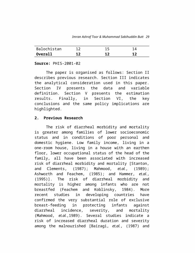
The Lahore Journal of Economics, Vol.8, No.1
Another important variable is distance from health facilities. The trend of this variable is positive which indicates that long distance from health facilities increases the incidence of diarrheal disease. Since this only concerns individuals who actually used the services, it cannot be considered to represent access for the population as a whole. For treatment, users of government services reported traveling slightly further than private services, although the proportions who traveled less than 5 km are very similar. For private diarrhea treatment, Balochistan and NWFP had a substantial proportion of users traveling over 5 km.7
The coefficient of per capita income is negative which illustrates that per capita income has a negative relation with diarrheal disease. This trend indicates that higher income is negatively associated with diarrheal disease. This result also shows that poor children are mostly affected by diarrheal disease due to non-availability of health facilities. The influence of poverty on socio-economic conditions rather than health condition is very pronounced. It is in its way related to the income effect. In other words, poverty and spending are directly related and directed towards the improvement of public health services25.
Theoretical calculations based on the above sample indicate that promotion of the flush system in the household can reduce diarrhea morbidity in the house. Acute and chronic diarrheal disease is related to inadequate waste removal. Efficient removal of waste from living areas is also likely to reduce the prevalence of skin infections, hepatitis and polio. Surprisingly, the urban dummy has a positive and significant sign, which illustrates that in the urban areas, the incidence of diarrheal disease is higher than rural areas. The problem of solid waste management has acquired alarming dimensions in urban areas, especially over the last decade. Before then, waste management was hardly considered an 25 According to the UNFPA report entitled, The State of World Population 1999: “Poverty is not confined to the poorest countries. Over a billion people are still deprived of basic needs. Of the 4.8 billion people in developing countries, nearly 3/5th lack basic sanitation. Almost 1/3rd have no access to clean water. A quarter does not have adequate housing. 1/5th have no access to modern health services”.
38
Imran Ashraf Toor & Muhammad Sabihuddin Butt
issue of concern as the waste could easily be disposed off in an environmentally safe manner within the general premises. Contaminated drinking water supply through municipal corporation may also increase the incidence of diarrhea in urban areas. Evidence suggests that waterborne disease contributes to background rates of disease not detected as outbreaks. The waterborne diseases include those transmitted by the fecal–oral route (including diarrhoea, typhoid, viral hepatitis A, cholera, dysentery) and dracunculiasis.26 The other variable ‘persons per room’ has also a positive significant sign. This proves that conjunction of the persons in the house can increase the incidence of diarrheal disease. The large number of persons per room may mean improperly managed environment conditions in the house. Owing to this, communal diseases can easily flourish in the unhygienic environment in the house. In this study, province is used as a category variable and the Punjab province is used as a reference category. The Sindh province dummy has a negative sign which shows less incidence of diarrheal disease as compared to the Punjab province.
Specification of urban and rural models which are represented in Table-4 and Table-5 have the same trend except some variables which have different signs and coefficients. For example in the urban model, tap water has a positive but insignificant coefficient, which may be due to the supply of water contaminated in the urban areas. In Pakistan, most of the people still do not have access to safe drinking water, the quality of tap water distributed by the state utilities is considered unsafe for drinking. In Karachi, where diarrhea is the leading cause of childhood death, municipally supplied water is heavily contaminated with fecal organisms.27 Children rank highest among the adversely affected groups of society owing to water contamination. Vulnerable as their immune system is, they
26 Global Water Supply and Sanitation Assessment 2000 Report.27Luby S, Agboatwalla M, Raza A, Mintz E, Sobel J, Hussain S, Husan R, Ghouri F, Baier K, Gangarosa G. Microbiologic Evaluation and Community Acceptance of a Plastic Water Storage Vessel, Point-of-Use Water Treatment, and Handwashing in Karachi, Pakistan. 47th Annual EIS Conference. April, 1998.
39

The Lahore Journal of Economics, Vol.8, No.1
almost always succumb to virulent diseases. Tap water in rural areas also has a positive insignificant sign but it has a smaller coefficient as compared to urban areas. This tendency indicates that tap water is less contaminated in the rural areas.
Table 3:Logistic Model of Diarrheal Disease(Both Areas)
Variables Coeffici t- Dependent variable: Diarrhea in the household (0-5) Constant -5.2360 -14.96***Young Children in the House age 0-5 0.0338 9.88***Young Children in the House age 6- 0.0057 1.97**Mother’s Education -0.0294 -2.36**Solid waste system -0.0311 -0.33 Covered Drainage System -0.0276 -0.21Household Size 0.0631 6.43***Tap water in the house 0.0444 0.47Hand pump in house 0.1567 1.64Distance Travel for Public /Private 1.8445 20.31***Log Household Per capita Income -0.0588 -1.50Flush System in the House -0.2947 -3.08***Persons per Room 0.0291 1.774*Urban 0.5258 6.09***Sindh -0.0806 -0.88NWFP 0.8756 8.41*** Balochistan 0.3540 2.84***Sample Size 6928Log Likelihood -LR statistic (16 df) 1524.34Probability (LR stat) 0.000McFadden R2 0.22
Source: Pakistan Integrated Household Survey 2001-02
Note: (i) * at 10 % level of significance (ii) ** at 5 % level of significance (iii) *** at 1 % level of significance
40

Imran Ashraf Toor & Muhammad Sabihuddin Butt
Mother’s education has a significant coefficient in the urban model and also negative sign in the rural model. This indicates that mother’s education is effective in both areas. Children whose mothers had more years of schooling were less likely to suffer from respiratory infection than children whose mothers were less educated, but mother’s education has a significant effect on the reduction of incidence of diarrhea. Children of educated mothers were more likely to be treated for either type of infection. No differences were detected between girls and boys in either disease incidence or treatment in our models.
The other very highly significant variable in the rural model is distance travelled for public/private health facilities. For diarrheal treatment, access actually appears to be slightly better for private services than for government services.28 This may be because parents are prepared to take their children somewhat longer distances for private services due to less satisfaction with government services. Children living less than one kilometer distance to the health service continued using it more frequently than others. This exhibits that health facilities are very poor and out of access for poor people in the rural areas. This is very obvious when the question of rural urban disparity arises. In Pakistan, it is frequently found that health facilities, be it curative or preventive, are somehow better provided in the urban centres and rural areas are often taken for granted with respect to the provision of facilities and hence are deprived of their basic rights. The variable ‘persons per room’ also has a positive coefficient, which determines conjunction of the persons in the house may increase the incidence of diarrheal disease in urban as well as rural areas. This conjunction can add immeasurably to discomfort and inconvenience in the house.
28 Pakistan Integrated Household Survey 2001-02
41

The Lahore Journal of Economics, Vol.8, No.1
Table 4: Logistic Model of Diarrheal Disease(Urban Areas Model)
Variables Coefficient
t-statistics
Dependent variable: Diarrhea in the household (0-5) years childrenConstant -5.7624 -8.72***Young Children in the House age 0-5 (Share)
0.0417 7.56***
Young Children in the House age 6-10 (Share)
0.0019 0.41
Mother’s Education -0.0324 -2.12**Solid waste system -0.0500 -0.41 Covered Drainage System -0.2364 -1.48Household Size 0.0524 3.34***Tap water in the house 0.1244 0.91Hand pump in house 0.0816 0.46Distance Travelled for Public /PrivateHealth Facilities
3.1445 10.77***
Log Household per capita Income -0.1104 -1.54Flush System in the House -0.2751 -2.00**Persons per Room 0.0517 1.90*Sindh 0.3286 2.37**NWFP 0.6907 4.06*** Balochistan -0.0180 -0.09 Sample Size 2761Log Likelihood -1090.43LR statistic (15 df) 496.54Probability (LR stat) 0.000McFadden R2 0.19
Source: Pakistan Integrated Household Survey 2001-02
Note: (i) * at 10 % level of significance (ii) ** at 5 % level of significance (iii) *** at % level of significance
42

Imran Ashraf Toor & Muhammad Sabihuddin Butt
Table 5: Logistic Model of Diarrheal Disease(Rural Areas Model)
Variables Coefficient
t-statistics
Dependent variable: Diarrhea in the household (0-5) years childrenConstant -5.3005 -
12.16***Young Children in the House age 0-5 (Share)
0.0302 6.78***
Young Children in the House age 6-10 (Share)
0.0079 2.06**
Mother’s Education -0.0233 -0.90Solid waste system -0.2003 -1.28 Covered Drainage System -0.0243 -0.07Household Size 0.0756 5.81***Tap water in the house 0.0634 0.44Hand pump in house 0.2887 2.37Distance Travelled for Public /PrivateHealth Facilities
1.6843 17.99***
Log Household per capita Income -0.0329 -0.68Flush System in the House -0.3693 -2.64***Persons per Room 0.0165 0.79Sindh -0.3921 -3.10***NWFP 0.9685 6.99*** Balochistan 0.6143 3.70***Sample Size 4167Log Likelihood -1618.51LR statistic (15 df) 1093.34Probability (LR stat) 0.000McFadden R2 0.25
Source: Pakistan Integrated Household Survey 2001-02
Note: (i) * at 10 % level of significance (ii) ** at 5 % level of significance (iii) *** at 1 % level of significance.
43
The Lahore Journal of Economics, Vol.8, No.1
6. Conclusion:
We have developed a model to estimate diarrheal disease employing household-level data collected from all over Pakistan using a relative aggregate indicator of illness in the household (the low rates of illness in our data allow us to successfully model diarrheal illness separately for children) and a cross-sectional approach. We find that several economic, engineering/behavioural and neighbourhood-level variables are associated with illness.
Among the engineering variables, poor reliability of the water supply is most strongly associated with diarrheal illness. The supply of water through a hand pump particularly in the rural areas results in higher incidence of diarrhea. Surprisingly, the water sources that supply urban households (government-piped water) have the highest interruption rates, making those households particularly vulnerable to diarrhea. Given the source of water, more educated households appear to engage in more defensive activities than a poorer household, but the effect of income on diarrhea is weak, to some extent because of the higher frequency of interruptions in the water supply. The availability of a covered drainage system (another variable, which we treat as given in the short term) appears to significantly increase defensive behaviour and decrease the risk of diarrheal illness.
Behavioural attitude is also a major factor in the reduction of diarrheal disease. For instance, diarrhea incidence is low with contaminated water, because households are careful in their personal hygiene, and boil water before drinking. In such a setting, an engineering intervention, such as improvement in water quality, could prove ineffective in lowering diarrhea rates because of the importance of behavioural factors. Poor reliability of the water supply may be associated with diarrheal illness. Interruptions in the water supply, particularly in the cities, are consistently found to interfere with defensive behaviour (washing hands after using the toilet), and result in higher incidence of diarrhea. Given the source of water, a
44

Imran Ashraf Toor & Muhammad Sabihuddin Butt
wealthier/more educated household usually appears to engage in more defensive activities than a poorer household. The availability of a washbasin near the toilet area can appear to significantly increase defensive behaviour and reduce the risk of diarrheal illness. Therefore, better water supply system can definitely reduce the mortality rate occurring due to diarrheal disease. Uncleaned toilets, filthy water over-flowing the drainage system, heaps of garbage lying here and there further make the health system deteriorate. In most of the cases of diarrheal disease the root cause is lack of hygiene.
Public interventions can exhibit varying levels of effectiveness in controlling the transmission of diarrheal disease, and a plentiful water supply and adequate sanitation appear to have a greater impact on diarrheal disease than improvements in water quality. Effectiveness in lowering disease rates, and particularly the severe and mortal cases, depends on broader preventive strategies, including water supply and sanitation, nutrition and education programmes. Thus, adequate sanitation practice, literacy and sound knowledge regarding the proper maintenance of hygienic conditions will undoubtedly reduce the incidence of diarrheal illness which ultimately results in child mortality.
But all these factors run in a vicious circle that is poverty, education and health. They are all inter related, rather inter-dependent. If the country really wants to control these fatal diseases, a blend or a synthesis of the efforts made by both the public and the private sectors is needed. This will avoid duplication of responsibilities as well as the risk factors and acquire a cost effective approach to solve the problem. Like all other government departments, the health department also suffers from overlapping problems in the delivery of services thereby resulting in inefficiency. In the specific case of Pakistan, economic development strategies that raise personal incomes and education do not necessarily guarantee lower rates of diarrhea. Some other measures should also be taken to control diarrhea in the future.
45

The Lahore Journal of Economics, Vol.8, No.1
References
Alberini, A.; G.S. Eskeland, A. Krupnick and G. McGranahan, 1996, “Determinants of Diairheal Disease in Jakarta”, Policy Research Working Paper # 1568. The World Bank.
Ashworth, Ann, and R. G.A. Feachem, 1985, "Interventions for the Control of Diarrheal in Young Children: Weaning Education", Bulletin of the World Health Organization 63: 1115-27
Bairagi, R.; M.K. Chowdhury; Y.J. Kirn; G.T. Curlin; and R. Gray, 1987, “The Association between Malnutrition and Diarrhea in Rural Bangladesh”, International Journal of Epidemiology 16: 477-481
Baitazar, J., J. Briscoe, V. Mesola, C. Moe, F. Solon, J. VanDerslice, and B. Young, 1988, “Can the Case-Control Method be Used to Assess the Impact of Water Supply and Sanitation of Diarrhea? A study in the Philippines”. Bulletin of the World Health Organization. 66 (5), 609-621.
Barros, F.C., C.G. Victora, J.P. Vaughan, H.J. Estanislaw, 1987, “Infant Mortality in Southern Brazil: A Population Based Study of Causes of Dealth,” Archives of Diseases in Childhood 62: 487-90.
Briscoe and John, 1984, “Intervention Studies and the Definition of Dominant Transmission Routes”, American Journal of Epidemiology. 120, 449-455.
Esrey, S.A., R.G. Feachem, and J.M. Hughes, 1985, “Interventions for the control of diarrhoeal diseases among young children: Improving water supplies and excreta disposal facilities”. Bulletin of the World Health Organization. 43 (4) 757-772.
Feachem, R. G.A. and M.A. Koblinsky, 1985, “Interventions for the Control of Diarrheal Diseases among Young
46
Imran Ashraf Toor & Muhammad Sabihuddin Butt
Children: Promotion of Breastfeeding”, Bulletin of the World Health Organization 62: 271-291.
Hammer, J.S.; Nabi Ijaz; and Cercone K.A., 1995, “Distributional Effects of Social Sector Expenditure in Malaysia, 1974-89”, In H. Chenery and T. N. Srinivasan (eds) Handbook of Development Economics. 1. Chapter 14, Elsevier Science Publishers.
Mahmood D.A., R.G.A. Feachem, and S.R.A. Huttly, 1989, “Infant Feeding and Risk of Severe Diarrhoea in Basrah, Iraq”, Journal of Tropical Paediatrics 33:319-25.
Martines, J., M. Phillips, and R.G.A. Feachem, “Diarrheal Diseases” pp. 91-116 in D.T. Jamison, W. H. Mosely, A.R. Measham, and J. L Bobadilla, eds., 1993, Disease Control Priorities in Developing Countries. Oxford University Press: New York (for the World Bank).
Murray, C.J.L., and A.D. Lopez, 1994, “Global and Regional Causes of death: Patterns in 1990”, Bulletin of the World Health Organization. 72 (3), 447-480.
Stanton, B. F. and J.D. Clements, 1987, “An Education Intervention for Altering Water-Sanitation Behaviours to Reduce Childhood Diarrhoea in Urban Bangladesh: II. A Randomised Trial to Assess the Impact of the Intervention on Hygienic Behaviours and Rates of Diarrhea”, American Journal of Epidemiology 125: 278-282.
47

Umer Khalid
Opportunities and Challenges for Pakistanin an Era of Globalisation
Umer Khalid*
Abstract
The study analyses the degree of integration of Pakistan’s economy in global trade and financial flows. Pakistan’s integration into the global economy gained momentum in the late 1980s and early 1990s when it adopted more open and liberal policies as part of stabilisation and structural adjustment programmes negotiated with the IMF and World Bank. The paper presents an overview of Pakistan’s economy in the before and after period, it will specifically examine the trade performance from the 1980s onwards to see the progress made towards the integration of the Pakistani economy into the world economy. It will look into the opportunities that Pakistan is likely to gain in a more globalised world, with special focus on the textile and clothing sector and the potential growth in this sector after the abolition of the Multi Fibre Arrangement (MFA) in 2005. New challenges that may emerge in a more open trading environment will also be discussed.
1. Introduction
Globalisation broadly defined as the free movement of goods, services, people and information across national boundaries has become a widely debated topic in recent years. Developing countries embrace Globalisation for a variety of reasons. Firstly, foreign investment provides *The author is Trainee Officer at the National Institute of Banking and Finance, State Bank of Pakistan, Islamabad. Author’s Note: The views expressed in this paper are the author’s own and do not reflect those of the State Bank of Pakistan. The author wishes to thank Usman Qadir, Staff Economist at the Pakistan Institute of Development Economists and Feyza Bhatti, Research Fellow at Mahbub ul Haq Human Development Centre for their valuable comments on an earlier draft of the paper.
45

The Lahore Journal of Economics, Vol.8, No.1
more jobs, new production technologies, infrastructure improvements and a source of capital for local entrepreneurs. Domestic businesses gain access to both cheaper inputs and much larger markets for their products. The removal of trade barriers expands the range of choices available to consumers and places downward pressure on prices thereby raising the real value of workers’ earnings. Globalisation and liberalisation present many new opportunities for developing countries such as Pakistan, viz. higher growth through export expansion and improvements in their balance of payments situation. A World Bank study (Dollar and Kraay 2001) shows that countries with higher integration in the world economy over the past two decades ending in the late 1990s achieved higher growth in incomes, longer life expectancy and better schooling.
Pakistan has traditionally pursued a mixed economy approach to development focusing on import substitution with a dominant role of the public sector. The 1960s saw a period of more open and liberal policies being followed where the private sector was encouraged to play a greater role. However, this trend was reversed in the seventies which was characterised by an increasing domination of the public sector in the economic activities of the country. By the second half of the eighties, Pakistan was faced with high macro imbalances as a result of the growing inefficiency and losses in the public sector. It was against this backdrop that the government was forced to enter into stabilisation and structural adjustment programmes with the International Monetary Fund (IMF) and the World Bank in 1988. These reforms encompassed a wide range of measures comprising stabilisation, structural adjustments and institutional reforms aimed at reducing the fiscal and balance of payments deficits. The stabilisation measures recommended included reduction of subsidies, upward adjustment of user charges, expenditure curtailment and tax reforms, sharp credit restraints and a reduction of the monetisation of the fiscal deficit. Structural adjustment worked towards removing the distortions present in the economy due to the
46

Umer Khalid
excessive role of the public sector in economic activities through deregulation and opening up the economy to foreign investment.
The paper will present an overview of the level of integration of Pakistan’s economy into the world economy and look into the opportunities and challenges that are faced by the country. Section 2 will present a brief overview of Pakistan’s economy during the past two decades, i.e., the eighties and the nineties. It is widely accepted that Pakistan’s integration into the global economy gained momentum in the late eighties and the early nineties so it will be instructive to have a look at the economic performance of the country before and after this phenomenon. The trade performance of the economy will also be reviewed with special reference to the textile and clothing sector to export growth. Different indicators like the trade to GDP ratio, tariff rates, etc will be used to analyse the current and past level of trade and financial integration of Pakistan in Section 3. Section 4 will look into the opportunities that will accrue to Pakistan in a more open trading environment with a specific focus on opportunities likely to arise in the textile and clothing sector after the elimination of the Multi Fibre Arrangement (MFA) in 2005. New challenges that may emerge for Pakistan with reference to the textile and clothing sector will be examined in Section 5. Section 6 will end the paper with some concluding remarks.
2. Review of Pakistan’s Economy (1980-2000)
Pakistan is part of the South Asian region, which was home to over 1.3 billion people in 2000 (UN 1999). South Asia is regarded as one of the most underdeveloped regions of the world, where the average per capita income was just $ 440, slightly higher than the average for the low income countries at $ 410 but even lower than the average for Sub Saharan African countries (World Bank 2002). The region’s GDP represented just 1.9 per cent of the world GDP in 2000, whereas its share in world population was around 22.4 per cent.
47

The Lahore Journal of Economics, Vol.8, No.1
Pakistan with a population of 138 million was the seventh most populous country of the world in 2000 (Table 1), its population representing around 11 per cent of South Asia’s population. Pakistan’s economy averaged a GDP growth rate of only 3.7 per cent during the 1990s, as compared to 6.3 per cent during the eighties. While the growth in the agricultural sector remained the same during the nineties, the period saw a substantial decline in the growth in other sectors, i.e., industry, manufacturing and services, contributing to the overall decline in the GDP growth for the 1990s. A structural transformation can be observed in Pakistan’s economy over the past two decades with the contribution of the agricultural sector steadily declining and the value added by the services sector rising during this time period. Presently, the services sector is the largest contributor to GDP adding 51 per cent to the national income of the country (Table 2) and is the sector with the greatest potential for future growth. This is followed by the agriculture sector, which added 26 per cent of value to the GDP in 2000.
In 2000, Pakistan had a per capita GDP of around $ 440 placing it in the low income category29. The real GDP per capita in Pakistan grew at an average of only 1.2 per cent during the nineties, which was much less than the population growth rate during that decade. This brought an increase in the poverty levels prevalent in the country; in 1990-91, 21 per cent of the households were below the poverty line while by 1998-99 the poverty level had increased to 33 per cent (MHHDC 2001).
29 According to the World Bank classification, countries having GNP per capita of less than $ 755 are considered low income countries.
48

Umer Khalid
Table 1: Basic Economic Indicators of PakistanPopulation (millions)
1990 1062000 138
Population growth (%)1990-1995 2.71995-2000 2.6
GDP per capita (US $)1980 30019902000 440
Real GDP growth (%)1980-1990 6.31990-2000 3.7
Real GDP per capita growth (%)1990-2000 1.2
Source: World Bank (2002), MHHDC (2001), UNDP (1993 & 2002).
Table 2: Structure of ProductionValue Added to GDP by
1980
1990
2000
Average annual growth (%)
1980-1990
1990-2000
Agriculture 31 26 26 4.3 4.4 Industry 25 25 23 7.3 3.9 Manufacturing 16 17 15 7.1 3.5 Services 44 49 51 6.8 4.4Source: World Bank (2002).
Trade Performance of Pakistan
It can be seen clearly from Table 3 that throughout the past two decades Pakistan’s imports have exceeded its exports. Pakistan’s exports stood at $ 9.6 billion by the year 2000, while its imports stood at around $ 11.8 billion,
49

The Lahore Journal of Economics, Vol.8, No.1
implying a trade deficit of $ 2.2 billion. However, the trade deficit as percentage of the GDP has come down significantly from 12 per cent in 1980 to 3 per cent by 2000, as exports have increased while at the same time imports have declined. During the eighties, Pakistan’s exports recorded a high growth of 11.1 per cent per annum, as a result of which exports had grown from 12 per cent of the GDP in 1980 to 16 per cent of the GDP by 1990. The growth in exports fell to half that rate in the nineties, while imports grew by an annual average rate of just 0.7 per cent during this decade.
The share of merchandise exports in total exports has been steadily rising during the past two decades; merchandise exports accounted for about 96 per cent of total exports in 2000. A further breakdown of merchandise exports reveals that manufactures were 85 per cent of merchandise exports in 2000. In 1980, manufactures formed only 48 per cent of the merchandise exports, while 24 per cent were food exports and agricultural raw materials were 20 per cent. Thus, we can see a shift away from food and agricultural raw materials towards manufactures during the past two decades. Food and agricultural raw materials formed only 11 and 3 per cent respectively of merchandise exports. However, the bulk of the manufactured items still fall into the category of traditional labour intensive goods.
Table 3: Trade statistics for Pakistan1980
1990
2000
Average annual growth (%)
1980-1990
1990-2000
Total exports ($ million)
2958
6217
9575
11.1 5.4
Total imports ($ million)
5350
9351
11762
7.3 0.66
Imports as % of GDP
24 23 19 4.1 1.1
Exports as % of GDP
12 16 16 0.3 -0.9
50

Umer Khalid
Trade balance (% of GDP)
12 7 3 - -
Source: World Bank (2002).Table 4: Structure of Exports
1980 1990 2000Total exports ($ million) 2958 6217 9575Merchandise exports ($ million)
2588 5589 9173
Merchandise exports as % of total exports
87.5 89.9 95.8
% of Total Merchandise Exports
Food 24 9 11Agricultural raw materials 20 10 3Fuels 7 1 1Manufactures 48 79 85
Source: World Bank (2002).
Increasing trade integration requires a well-diversified export base, both geographically and by product. Dependence on a few export products and markets increases the risks associated with market fluctuations. Pakistan’s export base has however, not seen the level of export diversification that is typical of a globalised economy during the past ten years after it opened its economy with the introduction of liberalisation and trade reforms. It is still concentrated on a few low value added commodities, namely the textiles and clothing products. Here it can also be seen that the major part of Pakistan’s textile exports is of cotton yarn while the leading exporters of textile and clothing have increased their share of value addition (Javed and Haseeb 2001). This lack of export diversification has resulted in rising concentration indices during the 1990s (Husain 2001).
Export diversification can also be seen in terms of the destination of exports. Here also it can be seen that the major share of Pakistan’s textile exports goes to the
51

The Lahore Journal of Economics, Vol.8, No.1
United States, European Union, Canada and Japan. Exports to these economies are mostly in the form of quotas with the exception of Japan.
The Importance of Textile and Clothing Exports for Pakistan’s Economy
Pakistan is heavily dependent on its textile sector for export earnings. As shown in Table 5, the share of textile and clothing sector in the exports of Pakistan has been steadily rising during the past two decades; it was 46 per cent of total merchandise exports in 1980-84 while by the next 5 years its share had risen to over 53 per cent. In the first half of the nineties, the share of the textile and clothing sector had reached around 70 per cent of Pakistan’s total exports, while the second half of the nineties did not see a significant increase in the share of this sector in total exports. The abolition of the MFA is thus very important for the textile sector of Pakistan, as Pakistan will be in a position to increase its textile exports and consequently its export earnings in a quota free world after 2005.
Table 5: Shares of Textiles and Clothing in Total Exports of Pakistan
Year Share in Total ExportsTextiles Clothing Textile and
clothing1980-84 39.824 6.32 46.1441985-89 42.458 13.34 53.3661990-94 49.212 19.886 69.0981995-99 52.062 21.524 73.586
Source: Malik (2000).
The share of Pakistan’s textile and clothing exports in the world total has been rising moderately. The textile exports during the eighties were around 2 per cent of the world’s textile exports, which increased to over 2.9 per cent in the nineties (Table 6). The share of Pakistan’s clothing exports on the other hand, have seen a higher
52

Umer Khalid
increase in the past two decades. Between 1980-84 they accounted for just 0.4 per cent of the world’s total exports of clothing, while by the first half of the nineties they had grown to around 1.1 per cent. However, in the later part of the nineties, clothing exports registered a slight decline.
Table 6: Performance of Textile and Clothing Exports of Pakistan Internationally
Years Textile Exports% Share of Pakistan in World Total
Clothing Exports% Share of Pakistan in World Total
1980-84 2.03 0.411985-89 2.03 0.721990-94 2.92 1.081995-97 2.9 1.06Source: Malik (2000).
The world trade in clothing has been governed by the Multi Fibre Arrangement since 1974 encompassing a range of quantitative restrictions and has fallen outside the purview of the General Agreement on Tariffs and Trade (GATT). The MFA has been used by the developed countries to restrict exports from selected developing countries including Pakistan but it does not restrict exports across the developed countries (Mahmood 1999). In order to protect their domestic textile and clothing industry from exports of developing countries,’ the developed countries followed restrictive trade policies in the form of high tariffs, tariff escalation and non-tariff barriers (Musleh-ud Din and Abbas 1999). One of the main obstacles in the growth of textile exports from the developing countries towards the developed countries has been an array of quantitative restrictions mainly in the form of a regime of quotas on exports and imports.
53

The Lahore Journal of Economics, Vol.8, No.1
3. Level of Trade and Financial Integration of Pakistan between 1980-2000
Trade Integration
One of the main indicators used to measure the level of trade integration of a country into the world economy is the trade to GDP ratio, also known as the “openness ratio”. Countries that are highly integrated in the world economy tend to have a high trade to GDP ratio. However, bigger countries tend to have comparatively lower trade to GDP ratios than smaller countries because they have higher endowments of natural resources and greater opportunities for internal trade (World Bank 1997).
In Pakistan this ratio was 34.3 per cent during 1981-89 which increased to 38.7 per cent by 1990-98 (Table 7), signifying Pakistan’s higher level of trade integration during the nineties. It can also be observed that Pakistan’s openness ratios during both the nineties and the eighties were considerably higher than the South Asian average. Overall, as the figures show, South Asia was one of the least integrated regions in the world, its trade ratios even lower than those for the low income countries during both the eighties and the nineties. The East Asia and Pacific region had trade ratios in excess of 60 per cent during the nineties showing the higher level of trade integration of these countries.
Table 7: Trade to GDP Ratios of Pakistan
1981-89
1991
1997
1990-98
Average Annual
Change (%)1981-89
1990-98
South Asia 19.4 - - 26.3 0.1 3.6 India 14.5 13.
9427.08
21.9 1 4.7
Pakistan 34.3 34. 39. 38.7 -0.2 0.3
54

Umer Khalid
96 95East Asia & Pacific
45.8 - - 60.1 1 5
Low income 26.5 - - 40.3 1.9 5.3Source: MHHDC (2001), Kemal (2001)
Trade to GDP ratios measured in nominal terms, however, are highly sensitive to movements in real exchange rates. A depreciation in the real exchange rate of a country would increase its trade to GDP ratio as it would lead to higher prices of exports and imports relative to the GDP price deflator and vice versa. Therefore, comparisons among countries using market exchange rates may be misleading as non-tradable goods tend to have lower relative prices in developing countries than in developed countries (World Bank 1997). The trade to GDP ratios can be re-estimated using purchasing power parity adjusted (PPP) GDP to overcome this problem. A moderate rise can be observed in the trade to GDP ratios adjusted for PPP for the South Asian countries as most of the region’s currencies including the Pak Rupee have undergone depreciation during the nineties. In Pakistan’s case, a very slight rise is observed in the trade ratio (Ibid).
Another indicator of the degree of trade integration is the import tariff rate, which serves as a proxy for the difference between domestic and international prices. The maximum tariff in Pakistan came down from 225 per cent in 1986-87 to 70 per cent in 1994-95, which was further reduced to 35 per cent by 1997-98 (Kemal 2001). The average tariff rate has come down to 11 per cent in 2000-01 from 51 per cent a decade earlier (Husain 2001).
Pakistan has also made progress in eliminating and reducing non-tariff barriers to trade. Import licenses have been abolished for all goods except those on the negative list30 or restricted list31. The scope of lists specifying
30 The negative list allows free imports of capital goods and industrial raw materials.31 Restricted list contains importable products by specified importers and industrial consumers only.
55

The Lahore Journal of Economics, Vol.8, No.1
restricted/ prohibited imports has been sharply reduced. Presently, there are only 32 products on the negative list and import of 28 products is restricted because of health and safety reasons (Kemal 2001).
Financial Integration
The degree of Pakistan’s integration into the global financial and capital markets can be measured in several ways. The most widely used indicator of financial integration is the ratio of Foreign Direct Investment (FDI) and portfolio flows to GDP.
Pakistan’s efforts to integrate into the world economy have not only encompassed trade reforms but also the liberalisation of the financial sector. The opening up of the domestic financial markets is very important to attract increased levels of foreign capital to ease the balance of payments situation and provide increased capacity to import. Financial integration can boost growth by raising domestic investment, which can be financed by foreign savings. It can shift the investment mix towards projects with a higher rate of return, through knowledge spillovers (especially from FDI). It stimulates financial sector deepening, competition and development. Financial sector integration allows individuals and firms to insure themselves against adverse developments in their home markets thereby smoothening temporary declines in income.
FDI flows to Pakistan have increased markedly during the 1990s. From an average of $ 120 million in the 1980s, it reached an average of $ 483 million during the 90s (Table 8), as a result of the liberalisation efforts and opening up of the economy during the early part of the nineties. Despite the higher flows of FDI during the nineties, the FDI to GDP ratio for Pakistan was considerably low in that time period although it had improved significantly from the ratio during the 80s. However, cross country comparisons reveal that in 1980 Pakistan received 34.1 per cent of the FDI flows to the
56
Umer Khalid
South Asian region which had declined to only 13.7 per cent by 1999 (MHHDC 2001).
FDI flows to Pakistan have mostly gone to natural resource exploration mainly in the oil and energy sector. FDI flows to export oriented industries have been limited in the case of Pakistan, e.g., by the mid nineties less than $ 100 million had been invested in the Karachi Export Processing Zone since it was set up in the early 1980s (Ibid).
Table 8: Foreign Direct Investment in Pakistan
US $ million % of GDP Average annual
growth in value (%)
Average
1980-89
Average
1990-99
Average
1980-89
Average
1990-99
1980-89
1990-99
South Asia
256.2 2151.4a
0.08 0.44a 25 31.3a
India 104.7 1424.3a
0.04 0.37a 85 57.1a
Pakistan
107.9 500.7 0.33 0.88 27 13
East Asia & Pacific
3966.8
41326.5a
0.67 2.67a 26.9 26.2a
a: 1990-98Source: MHHDC (2001).
While the main source of capital flowing into the developing countries is Foreign Direct Investment (FDI), portfolio equity flows form another component of private non-debt capital coming to such countries. While the benefits of FDI inflows to the economic growth of host countries is clearly acknowledged empirically (Blomstrom et
57

The Lahore Journal of Economics, Vol.8, No.1
al.1992), evidence on the role of portfolio flows is not so clear (Claessens et al. 1995). Portfolio investments are more volatile than FDI; they are mostly short-term assets that can be withdrawn quickly. Moreover, equity flows due to their volatility render countries more exposed to shocks and disturbances in international markets, such as changes in interest rates and exchange rates. The East Asian financial crisis of 1997 clearly illustrated that countries with high levels of portfolio investments are more vulnerable to quick outflows of capital.
In Pakistan, portfolio flows were negligible in the early part of the nineties, until 1993 (Figure 1). They reached a peak of $ 1.35 billion in 1994 but have seen a declining trend since then due to the worsening macroeconomic situation and political instability prevalent in the country.
Portfolio flows coming to Pakistan formed only a negligible 0.01 per cent of GDP in the early part of the 1990s (Table 9), much below the average for developing countries. This ratio had improved to around 1 per cent of GDP by the nineties due to the greater inflows of portfolio investments coming into the country resulting from the liberalisation of the financial markets.
Figure 1: Portfolio equity flows to Pakistan (US $ billion)
58

Umer Khalid
Source: MMHDC (2001).
59

The Lahore Journal of Economics, Vol.8, No.1
Table 9: Ratio of Portfolio Inflows to GDP
1980-84 (%) 1990-94 (%)South Asia 0.00 0.33 India 0.00 0.62 Pakistan 0.01 0.94Developing countries 0.08 0.42
Source: World Bank (1997).
4. Opportunities for Pakistan
Globalisation offers many new opportunities for a country such as Pakistan. It would have greater opportunities to increase its growth through higher exports and inflows of investment, transfer of technology creating jobs for the people. The greatest gains for Pakistan will come from trade liberalisation in products, in which it enjoys a comparative advantage, namely, the textile and clothing sector. This sector is presently contributing more than 70 per cent to the export earnings of the country and providing employment to about 38 per cent of the industrial labour force (Javed and Haseeb 2001). The abolition of the Multi Fibre Arrangement in 2005 thus presents Pakistan with opportunities to expand its export base and diversify its export markets.
World trade in textiles and clothing has been governed by the Multi-Fibre Arrangement (MFA) for the past several decades. The MFA was a system of bilaterally negotiated agreements under a multi-lateral framework which was primarily meant to restrict textile and clothing exports from the developing countries to the developed countries. While tariff barriers were clearly a part of the MFA, quantitative restrictions in the form of a strict regime of export and import quotas on trade in textiles and clothing were the main instruments used by the developed countries to restrict exports from the developing countries. Another feature of the MFA was that the tariffs on textile and clothing products tended to increase with the stage of processing. For example the average tariff on fibers in industrial
60

Umer Khalid
countries was about 1 per cent while that on clothing was often as high as 20 per cent. Such tariff escalation was intended to protect high value added industry in the developed countries (Musle ud Din and Abbas 1999).
The key element of the Uruguay Round Agreement on Textile and Clothing is the phased elimination of the MFA over a 10-year period proceeding in four phases. According to this formula, by 1 January 1995, 16 per cent of imports of textiles and clothing should be quota free. By 1 January 1998, another 17 per cent must be made quota free and by 1 January 2002, 18 per cent more fall outside the quota regime. The final 49 per cent will be integrated on 1 January 2005 (SCCI 2000). With the implementation of the World Trade Organization (WTO) Agreement, Pakistan’s exports would receive significant tariff reductions from the developed countries (DCs) and less developed countries (LDCs). Tariffs on textile and clothing in LDCs will decline by 8.9 per cent, in agricultural products by 5.1 per cent, minerals and fuels by 13.3 per cent and miscellaneous manufactures by 7.5 per cent (Mahmood 1999). In the DCs tariffs on basic manufactures are expected to fall by 2.2 per cent, in agriculture by 3.6 per cent and in miscellaneous manufactures by 2.5 per cent. Thus the average post Uruguay Round tariffs for these products are likely to be 3.4 and 10.8 per cent respectively (Ibid).
Pakistani exports would, therefore, face a weighted average post Round tariff of 6.9 per cent in DCs’ markets and 9.1 per cent in LDCs’ markets. Pakistan’s total merchandise exports to the DCs and LDCs would thus gain a weighted average tariff reduction of 2.4 per cent in agriculture and 6.9 per cent in miscellaneous manufactures (Mahmood 1999). Ingco and Winters (1995) estimate that the gains for Pakistan will be more than $ 500 million with the removal of the MFA. Mahmood (1999) puts these gains at $ 1-1.3 billion taking into account the tightness with which the MFA has bound Pakistan.
An important change expected from the ATC will be the reduction in non-tariff barriers. The dismantling of the
61

The Lahore Journal of Economics, Vol.8, No.1
MFA will do away with the quota system which presently hampers Pakistan’s textile and clothing exports that are mainly directed towards quota countries and whose quota utilisation rates are very high (Mahmood 1999). The major share of Pakistan’s textile exports goes to the United States, European Union, Canada and Japan. Exports to these economies are in the form of quotas with the exception of Japan. Pakistan will thus be in a more favourable position to increase its exports of textiles and clothing to these markets. Low and Yeats (1994) show that the proportion of Pakistan’s exports to be affected by existing NTBs should fall from 60 per cent in 1992-93 to 8 per cent as a result of the implementation of the Agreement on Textile and Clothing (ATC).
62
Umer Khalid
Box 1: Agreement on Agriculture (1994)Proposals for Reduction in Support & Protection
Developed Countries
Developing Countries
Import Tariff: Average cut for all agricultural products
36 % 24 %
Minimum cut per product 15 % 10 %Domestic Support Total cuts for the sector 20 % 13 %Export Subsidies Cut on value of subsidies 36 % 24 % Cut on subsidized quantities 21 % 14 %Time allowed for implementation
1995-00 1995-04
6 years 10 yearsSource: The Nation, December 30, 2002
5. Challenges
The year 2005 will mark the end of the Multi Fibre Arrangement, which has restricted textile and clothing imports from the developing countries into the markets of developed countries. The system of quotas under which exports of textiles and clothing were subjected to quantitative restrictions will be abolished and will be replaced by a tariff based system. The developed countries will have to cut their import tariffs on agricultural imports by an average of 36 per cent, while the developing countries will have to cut their import tariffs by an average 24 per cent (Box 1). The domestic textile industry should be prepared for a more competitive environment after 2005, both in the local market as well as in international markets. The industry must strive to enhance competitiveness by promoting
63

The Lahore Journal of Economics, Vol.8, No.1
efficient utilisation of resources like raw materials and financial and human capital.
Pakistan is one of the leading producers of raw cotton providing it with a strong base for the growth of its textile and clothing. However, Pakistan has not been able to fully exploit its traditional edge (Musleh ud Din and Abbas 1999). The main emphasis in the textile industry of Pakistan has been on spinning activity. The major share of the yarn produced is exported to countries such as Japan, Hong Kong and South Korea. These countries having well developed textile industries convert this yarn into high value added products which fetch a high price on the international markets. There is a need to diversify the export base away from the traditional cotton based products to synthetic fibers. To maximise gains from trade, Pakistan should focus on value addition rather than intermediate products.
The textile and clothing industry in Pakistan has mainly grown under an umbrella of high tariffs, subsidies, concessionary finances, subsidised cotton prices and other incentives which the government has been providing from time to time. However, despite enjoying this high level of protection, the industry has not been able to improve its efficiency and competitiveness. In order to be competitive at the international level the cost structure needs to be rationalised, productivity increased and the quality of the final product needs to be improved (Musleh ud Din and Abbas 1999). With the implementation of the Agreement on Agriculture, Pakistan will have to reduce such subsidies to the textile sector.
Under the Agreement on Agriculture there is also a minimum market access commitment that 3 per cent of consumption of agricultural products of developing countries must be importable without any quantitative restrictions. This percentage is supposed to rise to 5 per cent over six years beginning from 1 January 1995. However, Pakistan is so far exempted from this requirement as it has invoked
64

Umer Khalid
Article XVIIIB, under which a country having balance of payments problems is exempted from this prohibition.
Market access for the textile and clothing exports of the developing countries to the developed countries’ markets can be restricted after the abolition of the MFA by the use of the safeguards agreement. Under this agreement temporary deviations from WTO disciplines are permitted during the period of transition if an import surge hurts or threatens to hurt domestic industry (SCCI 2000). Imports from developing countries can be prohibited if they are made using child labour. It is feared that developed countries will resort increasingly to these types of tactics to restrict imports from developing countries such as Pakistan in the post MFA period. The issue of child labour has been used to curtail the exports of stitched footballs from Pakistan, for instance.
Market access can also be denied to developing countries on the basis of non tariff barriers like Technical Barriers to Trade (TBT) which relates indirectly to environmental issues, for example, bans on use of azo dyes (Ibid). The Agreement on Sanitary and Phytosanitary (SPS) measures which encompasses a range of health standards applicable to agricultural commodities will pose problems for Pakistan. It will have to adjust to such standards in order to gain opportunities in the agricultural sector (Mahmood 1999).
To fulfil its commitments on Trade Related Intellectual Property Rights (TRIPS), Pakistan will have to modify its existing regime of intellectual property rights protection and establish an effective enforcement mechanism, which can prove to be quite challenging. Furthermore, with the implementation of TRIPS, it is feared that protected firms (mostly multinationals) working in the pharmaceutical sector will use their market power to raise prices and licensing fees. This will also reduce the access to technology for developing countries such as Pakistan, reducing its access to scientific and technological knowledge. Pakistan needs to promote
65

The Lahore Journal of Economics, Vol.8, No.1
indigenous technology by investing more in research and development.
There continues to be problems with the anti dumping agreement which may work against the interests of South Asian countries. For example, South Asian countries do not yet follow international accounting standards which are necessary to present defenses against anti-dumping investigations.
6. Conclusion
The level of Pakistan’s trade and financial integration has increased during the nineties as it has opened up its economy and followed a more liberal trade regime. However, this level of integration is still far lower than that achieved by similar developing countries. It can also be observed that the performance of Pakistan’s economy during the nineties (the period associated with greater integration into the global economy) has been lackluster as the economy was plagued with macro imbalances. In spite of this, exports have registered an increase while imports have declined during this period. A shift towards manufactured goods in the export basket can be observed but the export base continues to be concentrated in a few low value added items, namely textile and clothing products.
The greatest gains in globalisation for Pakistan will come from trade liberalisation in products, in which it enjoys a comparative advantage, namely, the textile and clothing sector. This sector is presently contributing more than 70 per cent to the export earnings of the country and provides employment to about 38 per cent of the industrial labour force. The MFA which has restricted exports of textiles and clothing from the developing countries such as Pakistan will come to an end in 2005, when the non tariff barriers like quotas will be replaced by tariffs. This will remove the quantitative restrictions on exports of these products currently in place and would thus afford greater opportunities for Pakistan to increase its exports to the
66

Umer Khalid
developed countries. However, this sector will become highly competitive after 2005 and Pakistani textile products will face increasing competition from the products of countries such as Bangladesh, China and India.
In order to survive in this more competitive environment, Pakistan needs to restructure its textile industry on modern lines while emphasising the quality of finished goods. In this regard, the government should implement international quality standards like ISO 9000 and ISO 14000 in the production of textile products. Efforts should be made to diversify into high value added products such as garments/ apparels making use of the cotton yarn currently being exported and synthetic fibres which fetch higher prices in international markets.
Overall, the potential gains from globalisation are numerous for a country such as Pakistan. In order to capture these gains, the textile industry would have to improve its efficiency levels to produce at lower costs than it presently does, while on the other hand it must also be prepared to face competition in the domestic market in which it presently enjoys a monopoly.
67

The Lahore Journal of Economics, Vol.8, No.1
References
Blomstrom, M., R. Lipsey and M. Zejan, 1994, What Explains the Growth of Developing Countries? In W.J. Baumol, R.R. Nelson and E.N. Wolff (eds)., Convergence of Productivity: Cross National Studies and Historical Evidence. Oxford: Oxford University Press.
Claessens, S. A. Demirguc-Kunt and A. Warner, 1995, Portfolio Capital Flows: Hot or Cold? World Bank Economic Review, 9 (1), 153-74.
Dollar, David and Aart Kraay, 2001, Trade, Growth and Poverty. Policy Research Paper No. 2587, World Bank, Washington D.C.
Husain, Ishrat, 2001, How is Pakistan positioning itself for Challenges of Globalization? Mahbub ul Haq Human Development Review, 1(2), 101-111.
Ingco, M.D. and L.A. Winters, 1995, Pakistan and the Uruguay Round: Impact and Opportunities, A Quantitataive Assessment, Background Paper for Pakistan 2010 Report, World Bank, Washington D.C.
Javed, Attiya Yasmeen and Haseeb Ahmad Bhatti, 2001, How to live in Textile Quota Free World, Paper presented at the 16th Annual General Meeting and Conference of the Pakistan Society of Development Economists, Islamabad.
Kemal, A.R., 2001, Globalization and South Asia’, Mahbub ul Haq Human Development Review, 1(1), 61-75.
Low, P. and A. Yeats, 1994, Non Tariff Measures and Developing Countries: Has the Uruguay Round Leveled the Playing Field? Policy Research Working Paper 1353, World Bank, Washington, D.C.
68
Umer Khalid
Mahbub ul Haq Human Development Centre, 2001, Human Development in South Asia 2001. Karachi: Oxford University Press,.
Mahmood, Zafar, 1999, ‘WTO and Pakistan: Opportunities and Policy Challenges’, Paper presented at the 14th
Annual General Meeting and Conference of the Pakistan Society of Development Economists, Islamabad.
Malik, Afia, 2000, Demand for Textile and Clothing Exports of Pakistan, Research Report No. 180, Pakistan Institute of Development Economists, Islamabad.
Musleh ud Din and Kalbe Abbas, 1999, The Uruguay Round Agreement and Pakistan’s Trade in Textiles and Clothing, Paper presented at the 15th Annual General Meeting and Conference of the Pakistan Society of Development Economists, Islamabad.
SAARC Chamber of Commerce and Industry, 2000, WTO & South Asia Multilateral Liberalisation: A Collective Response from SAARC, Dhaka.
World Bank., 1997, South Asia’s Integration into the World Economy. Washington D.C.: World Bank,
World Bank, 2001, World Development Indicators 2001, CD-ROM.
United Nations, 1999, World Population Prospects: The 1998 Revision. Volume 1: Comprehensive Tables. Population Division, New York.
United Nations Development Programme, 1993, Human Development Report 1993. New York: Oxford University Press.
United Nations Development Programme, 2001, Human Development Report 2001. New York: Oxford University Press.
69

Muhammad Aslam Chaudhary & Amjad Naveed
Export Earnings, Capital Instability and Economic Growth in South Asia
Muhammad Aslam Chaudhary and Amjad Naveed*
I. Introduction
During the last two decades the role of international trade and flow of foreign capital have received considerable attention in the literature. Various studies have examined the impact of export instability and capital instability on economic growth in less developed countries.32 Empirical evidence supports the hypothesis of a deleterious impact of export instability on economic growth. However, some studies also indicated that the relationship was unstable but positive with economic growth.33 Yet there are no systematic empirical investigations into the implied links between export diversification and long-term economic growth, particularly in the case of South Asian countries. The major concern regarding export instability is that it retards economic growth. The theoretical rationale for the same is that export instability creates uncertainty in the supply of foreign exchange earnings, discourages capital formation and hence hampers economic growth.34 Another notion is that capital instability affects economic growth more significantly than that of exports instability.35 When a country uses other sources to finance development than * The authors are Associate Professor and graduate student respectively, Department of Economics, Quaid-I-Azam University, Islamabad, Pakistan. The views expressed are entirely those of the authors. They are thankful to Dr. S. M. Younis Jaffery and Dr. Shah Nawaz Malik for their valuable comments which helped to improve the study.32 See for example, MacBean (1966), Glezakos (1973), Vovodas (1974), Yotoupolos and Nugent (1976), Moran (1983), Savvides (1984) and Glezakos (1984).33 For unstable relationship see Moran (1983), Kenen and Voivodas (1972). For positive relationship between economic growth and export instability, see Savvides (1984), Yotoupolos and Nugent (1976), Knudsen and Parnes (1975) and MacBean (1966).34 See Nurkse (1958), MacBean (1966) and Glezakos (1984). 35 See Glezakos (1984, and Fosu (1991).
65

The Lahore Journal of Economics, Vol.8, No.1
export earnings, it leads to forced savings and foreign aid for funding investment projects, and then the speed and volume of capital formation determines economic growth, not the instability of export earnings. Thus, if there is instability in mobilising capital itself, it will be pernicious to output growth. As a result, it will affect economic growth more than export earning instability.36
Keeping in view the above theoretical linkages, the present paper is focussed on exploring linkages between export instability, capital instability and economic growth. A hypothesis will be tested whether instability associated with capital formation is affecting economic growth or fluctuations in export earnings are a bottleneck to economic growth. Moreover, impact of foreign exchange instability on economic growth will also be investigated. The analysis pertains to selected South Asian countries, which constitute more than 80% of the South Asian economy, i.e. Pakistan, India, Bangladesh, and Sri Lanka.
II. Methodology
Following the standard augmented production framework, [Fosu (1991), Balassa (1985), Feder (1982), Michaely (1977), and Maizels (1968)], output is not only a function of traditional new classical inputs of labour and capital but also of exports as stated below.
) ……………………..(1)
Where Q is real aggregate output; L and K are labour and capital inputs, respectively; and X denotes exports. Exports are usually employed to reflect international factors influencing economic growth. The beneficial effects of these international factors channelised through the export sector included the following.37
i. It encourages specialisation and competitiveness and therefore improves production.
36 See for detail, Hawkins, Epstein and Gonzales (1966) and Voivodas (1974).37 See detail Fosu (1991).
66

Muhammad Aslam Chaudhary & Amjad Naveed
ii. Advantage of large scale economies, and
iii. Adoption of relatively efficient techniques to compete in the world.
Based upon equation (1), the following equation (2) may be derived for estimation.
………………………. (2)
Where GQ, GL, GK and GRX are growth rates of output, labour, capital and exports, respectively.38 i (i= 1, 2, 3) measures the impact of the respective functional argument; 0 is the intercept; is the stochastic term. The complete model may be specified as:
…………………(3)
Where IK is capital intensity.
Vt is the error term.
To differentiate between capital instability and export instability, equation (3) may be written as:
…. (4)
Where IX is a measure of export instability.
Foreign exchange is regarded as vital to the economic growth of less developed countries (LDCs). The unavailability of foreign exchange is a major constraint in financing imports. It is also considered an important determinant of capital formation and GDP growth.39 Thus fluctuations in foreign exchange receipts are believed to generate obstacles to development and economic planning. To test this notion, we add a new variable in 38 GK is the gross domestic investment as a percentage of GNP.39 For detail see, Massell, Pearson and James (1972).
67

The Lahore Journal of Economics, Vol.8, No.1
equation (4) that is instability in foreign exchange reserves (IRS).
(5)
Where GL, GK and GRX are the growth rates of labour, capital and exports, and IX, IK and IRS are the measures of export instability, capital instability and instability in foreign exchange reserves, respectively. According to neo-classical theory, 1 and 2 are non-negative, and 3 are positive. The capital instability and the foreign exchange reserves instability may be more harmful than the usual hypothesis of export instability.
The results of the models are discussed in the next section.
III. Empirical Results
The present section consists of empirical findings pertaining to export instability, capital instability, foreign exchange instability and economic growth for selected South Asian countries i.e. Pakistan, India, Bangladesh and Sri Lanka.
3.1: Empirical Evidence pertaining to Pakistan
The results obtained by multiple regression estimates of equation (4) and equation (5) of our basic models are reported in Table 1 and 1.1, respectively. All regression equations are corrected for auto-correlation by applying the AR (1) and MA (1) process.
First equation (a) of Table 1 is estimated for all variables in equation (4), i.e. growth rate of labour force (GL), exports (GRX), and capital (GK) and exports and capital instability. Two variables, growth rate of capital (GK) and capital instability (IK), are found to be significant at the 10 percent level. The signs of capital instability ( IK) and export instability (IX), are both negative and IX is also insignificant. It appears that the capital instability variable
68

Muhammad Aslam Chaudhary & Amjad Naveed
(IK) and export instability variable (IX) are hampering the growth process. Capital instability has a larger magnitude than export instability for Pakistan. It confirms our hypothesis that capital instability (IK) is more harmful to GDP growth than export instability (IX).
To check the effect of IK separately, we omitted the variable IX and estimate equation (b) again. Results of equation (b) are slightly different from equation (1). R2
falls slightly but 't' values increase for capital instability, from 10 percent to 5 percent.40 The ‘F’ statistic also improves at a moderate level. Another variable, growth rate of exports (GRX), also becomes significant and it has a positive impact on economic growth. It means that the growth rate of exports promotes economic growth, whereas instability in capital stock is the major affecting variable for economic growth, compared to export instability.
To identify the separate effect of the export instability variable on economic growth, we dropped the capital instability variable (IK) and estimated equation (c). The coefficient of export instability has a negative sign but still insignificant. F Stat and R2 also fall slightly. If we compare equation (b) with equation (c), it becomes clear that the more effective variable in the growth equation is capital instability rather than export instability.41 This suggests that the economic growth of Pakistan is more affected by capital instability than by exports instability.
40 The variables IK and IX are highly correlated in equation (1). Multicollinearity problem may arise. Thus, when we dropped one variable the results improved. See Appendix Table: A.1.41 MacBean (1966) Fosu (1990) and Qaisrani (1996) also found the same results.
69

The Lahore Journal of Economics, Vol.8, No.1
Table 1: Pakistan: Export Instability, Capital Instability and Economic Growth: Results of Multiple
Regression Equation(Dependent Variable is GDP Growth)
Variables/equations
(a) (b) (c)
C -15.64(-1.17)
-15.005(-1.198)
-27.69(-2.62)**
GL 0.025(0.026)
0.041(0.044)
0.055(0.585)
GK 0.746(1.99)***
0.764(1.78)***
1.41(2.34)*
GRX 0.006(0.164)
0.62(1.971)***
0.01(0.234)
IK -2542.94(-1.781)***
-2378.71(-2.16)**
-
IX -667.23-0.40)
- -13.88(-0.018)
AR(1) 0.32(1.76)***
0.33(1.864)***
0.41(2.315)**
MA(1) - - -R2 0.51 0.49 0.43D.W. 2.09 2.11 2.12F stat 3.96 4.29 3.65
Note: Figures in Parentheses are t-statistics.
*Significant at 1 percent **Significant at 5 percent. ***Significant at 10 percent. GL = Average annual percent growth rate of the labour force. GK = Growth rate of Capital, measured as the mean annual gross domestic investment as a percentage of GDP. GRX = Average annual percent growth rate of exports. IK= Capital instability. IX = Export instability.
3.1.1. Foreign Reserves Instability and Economic Growth
70

Muhammad Aslam Chaudhary & Amjad Naveed
The results of equation (5) are reported in Table 1.1. Equation (a) is estimated for all variables including foreign exchange instability. Only a single coefficient, capital instability (IK) is significant at the 10 percent level and all other variables are insignificant. One reason could be that IK and IX are correlated and IK is also correlated with IRS.42 We dropped the IX and estimate the new equation (b), including IRS variable. Now three variables, growth rate of capital (GK), growth rate of exports (GRX) and capital instability (IK) are significant, and have the expected sign except instability in foreign reserves (IRS), which is insignificant. It means that by inclusion of IRS, results do not improve much. By dropping IK and including IX, equation (c) is estimated. But the IRS is still insignificant. Which suggests that foreign exchange reserves do seem to affect the economic growth of Pakistan.
To check the effect of instability in foreign exchange reserves on economic growth separately, we dropped the IK and IX variable in equation (d). The results indicate the same behaviour for IRS as in previous equation (b). It suggests that instability in foreign exchange reserves does not affect economic growth. It may be noted that the level of foreign exchange is not very high in Pakistan, which means that its dependency on reserves is negligible.
Our findings suggest that capital formation affects economic growth more than export earning instability. It implies that fluctuations in exports does lead to similar fluctuations in the ability to import because capital stocks of underdeveloped countries are limited. Thus, fluctuations in exports will lead to fluctuations in capital formation and hence affects the economic growth process. It might be more desirable to reduce the fluctuations in investable funds directly.
42 IRS and IK are correlated and may create problems of multicollinearity, so we dropped one variable and then estimated it. For details see appendix Table 1.
71

The Lahore Journal of Economics, Vol.8, No.1
Table 1.1: Pakistan: Export Instability, Capital Instability and Economic Growth: Results of Multiple
Regression Equation(Dependent Variable is GDP Growth)
Variables
(a) (b) (c) (d)
C -14.265(-1.058)
-14.15(-1.105)
-27.61(-2.55)*
-27.71(-2.66)*
GL 0.063(0.064)
0.058(0.061)
0.101(0.104)
0.10(0.11)
GK 0.723(1.029)
1.32(2.10)**
1.412(2.276)**
1.414(2.34)**
GRX 0.014(0.328)
0.38(2.01)***
0.013(0.309)
1.21(1.99)***
IK -2691.93(-1.73)***
-2564(-1.69)***
- -IX -556.509
(-0.324)- -59.64
(-0.033)-
IRS -237.46(-0.479)
-2.549(-0.531)
-119.038(-0.242)
-116.43(-0.245)
AR(1) 0.33(1.73)***
0.335(1.821)***
0.409(2.297)**
0.41(2.42)**
R2 0.51 0.50 0.46 0.45D.W 2.11 2.12 2.12 2.12F stat. 3.56 3.85 3.35 3.58
Note: Figures in Parentheses are t-statistics. of GDP.
GRX = Average annual percent growth rate of exports. IK= Capital instability. *** Significant at 10%. *Significant at 1 percent. **Significant at 5 percent. GL = Average annual percent growth rate of the labour force. GK = Growth rate of Capital, measured as the mean annual gross domestic investment as a percentage. IX = Export instability.
IRS = Instability in foreign exchange reserves.
72

Muhammad Aslam Chaudhary & Amjad Naveed
Table 2: India: Export Instability, Capital Instability and Economic Growth: Results of Multiple
Regression Equation(Dependent Variable is GDP Growth
Variables (a) (b) (c)C 41.40
(1.625)24.429(2.17)
4.44(0.95)
GL 6.22(1.64)
6.829(1.605)
0.048(1.654)
GK 1.196(1.372)
0.584(1.899)***
0.62(1.98)***
GRX 0.032(1.612)
0.46(1.92)***
-0.054(-1.34)
IK -31511.8(-2.323)**
-26097.51(-2.367)**
-
IX -6212.81(-0.761)
- -2497.61(-1.448)
AR(1) - - -MA(1) -0.904
(-3.79)*-0.963(-5.595)*
-
R2 0.51 0.50 0.46D.W. 1.96 1.97 2.201F stat. 3.54 3.97 3.39
Note: Figures in Parentheses are t-statistics.
*Significant at 1 percent. ** Significant at 5 percent. *** Significant at 10 percent. GL = Average annual percent growth rate of the labour force. GK = Growth rate of Capital, measured as the mean annual gross domestic investment as a percentage of GDP. GRX = Average annual percent growth rate of exports. IK= Capital instability. IX = Export instability.
3.2. Empirical Evidence pertaining to India
Equation (4) and equation (5) of the model are also estimated for India. The results are reported in Table 2 and 2.143. Equation (a) of Table 2 is estimated including all the 43 All the regression equations are corrected for autocorrelation by using AR (1) and MA (1) process.
73

The Lahore Journal of Economics, Vol.8, No.1
variables in equation (4). Only a single variable, capital instability (IK) is found to be significant at 5 percent. The signs of capital instability (IK) and export instability (IX) are both negative, but IX insignificant. Thus, it confirms our hypothesis that capital instability affects GDP growth more than export instability (IX) for India, which suggests that fluctuations in capital stock exist in the Indian economy and have effects on the economic growth of India. To retrieve the effect of IK separately, we omitted the variable IX and estimated equation (b). Results of equation (b) revealed that three variables are significant. The 't' values and F statistic also improved at a moderate level.44 Another variable, growth rate of exports (GRX) also becomes significant. It confirms our hypothesis that capital instability is negatively related to GDP growth. To carefully assess the effect of exports instability on growth, we dropped the capital instability variable (IK) and re-estimated equation (c).
The coefficient of exports instability has a negative sign but is still insignificant. F statistic and R2 also fall slightly. When we compare equation (b) with equation (c), it leads to the conclusion that the more effective variable in the growth equation is capital instability rather than exports instability, in the case of India.
3.2.1: Foreign Reserves Instability and Economic Growth
To check the effect of foreign exchange reserves instability on economic growth, we estimated equation (5) of the model. The results of equation (5) are reported in Table 2.1. First an equation is estimated for all variables including foreign exchange instability. The coefficients of three variables, growth rate of capital, capital instability and exports instability is significant at the 1 percent level. The coefficient of a new variable foreign exchange reserve instability (IRS) is insignificant. The insignificance of IRS may be due to high correlation with IX and IK as discussed in the case of Pakistan too. Thus, we estimated equation (b) by 44 Variables IK and IX are correlated, and when we omit one of them, the results improved. For details see appendix Table .A2
74

Muhammad Aslam Chaudhary & Amjad Naveed
omitting variable IX. Now four coefficients became significant, i.e. growth rate of labour, growth rate of capital, growth rate of exports and capital instability, which adds an important explanatory variable for the GDP growth of India. But foreign exchange reserve instability remained insignificant. The problem might be of correlation between IK and IRS. Thus, to remove that we have conducted sensitivity analysis and estimated another equation (c), by omitting IK and including IX.. It appears that three variables are significant including instability in foreign exchange reserves (IRS). In this equation we identify that foreign exchange instability also affects the economic growth of India.
To identify the effect of individual variables, eg: foreign exchange instability, we estimated another equation (d), by omitting variables IK and IX. The IRS was found significant at the 10 percent level. Two other variables, growth rate of labour (GL) and growth rate of capital (GK) are also significant, and signs of the coefficients are according to expectations.45 Thus, export instability is not proved as a major determinant to the Indian growth process. Our results of this regression are almost similar to that of Pakistan’s but the only difference is that foreign exchange reserves instability is also significant for India. Anyhow, it turns out that export instability has a minor contribution in affecting the growth of India. From the above evidence, we may conclude that exports earning instability would cause fluctuations in export earnings, a relatively unreliable source of foreign exchange earnings for investment purposes. Thus, it requires alternative funding sources in order to smooth out the uncertainties in investment funds. The impact of export instability on economic growth is through capital formation and foreign exchange needed for capital goods imports. Moreover, the stock of foreign reserves in India is greater than other South Asian countries,46 so greater reserves are more affected by fluctuations in capital 45 Qaisrani (1996) also found the same results for Pakistan. 46 For details see IFS (various issues), from 1970-80 the annual average reserves for India, Pakistan, Bangladesh and Sri Lanka are $3,095, $332, $248 and $174 million US $ respectively, and for 1970-99 for these countries are $8,181, $770, $898 and $678 million, respectively.
75

The Lahore Journal of Economics, Vol.8, No.1
formation and hence the greater impact on economic growth. Thus, it appears that in the case of India, fluctuations in capital formation and foreign exchange reserves will both be more detrimental to economic growth rather than fluctuations in export earnings47.
47 It may be noted that a major source of financing of foreign exchange is foreign loans.
76

Muhammad Aslam Chaudhary & Amjad Naveed
Table 2.1: India: Export Instability, Capital Instability and Economic Growth: Results of Multiple
Regression Equation(Dependent Variable is GDP Growth),
Variables (a) (b) (c) (d)C 5.387
(2.613)*0.323(0.18)
3.298(1.155)
0.62(0.175)
GL -0.96(-1.639)
1.028(1.67)***
1.0551(1.776)***
1.32(2.01)**
GK 0.201(2.82)*
0.397(8.51)*
0.277(2.816)*
0.47(2.86)*
GRX 0.035(1.102)
0.35(1.834)***
0.017(0.488)
0.04(0.97)
IK -2860.51(-3.539)*
-1215.039(-4.123)*
- -
IX -2338.89(-3.27)*
- -1823.43(-1.56)
-
IRS -240.19(-0.741)
-383.88(-1.304)
-371.087(-1.77)***
-586.9(-1.95)***
AR(1) - - - -0.38(-1.79)***
MA(1) -0.989(-2.814)
-0.98(-3.578)*
-1.39(-5.68)*
-
R2 0.66 0.73 0.64 0.69D.W 1.98 1.91 1.95 2.05F stat. 4.73 4.59 10.16 3.92
Note: Figures in Parentheses are t-statistics.
*Significant at 1 percent. **Significant at 5 percent. ***Significant at 10 percent. GL = Average annual percent growth rate of the labour force. GK = Growth rate of Capital, measured as the mean annual gross domestic investment as a percentage of GDP.GRX = Average annual percent growth rate of exports.
77

The Lahore Journal of Economics, Vol.8, No.1
IK= Capital instability. IX = Export instability. IRS= Instability in foreign exchange reserves.
3.3: Empirical Evidence pertaining to Bangladesh
To investigate the hypothesis that capital instability is more harmful than export instability to economic growth for Bangladesh, we estimated equation (4) and equation (5) of the model. The results of these equations are reported in Tables 3 and 3.1.
First, equation (a) of Table 3 is estimated by using all explanatory variables of equation (4). On the basis of 't' values, the results indicate that just a single coefficient of capital instability is significant at the 5 percent level of significance. All other variables are insignificant. This means capital instability is affecting economic growth of Bangladesh more than export instability.
Table: 3. Bangladesh : Export instability, capital instability and economic growth: Results of
multiple regression equation(Dependent variable is GDP growth)
Variables (a) (b) (c)C 5.146
(0.925)1.225(0.279)
-4.106(-0.818)
GL 1.107(1.587)
0.721(1.128)
1.345(1.748)***
GK 0.230(0.724)
0.358(1.681)***
0.619(2.588)*
GRX -0.014(-0.261)
0.37(2.02)***
0.32(1.85)***
IK -1341.52(-1.818)**
-1247.06(-1.813)***
-
IX -2012.84(-0.965)
- -533.82(-0.248)
AR(1) - -0.57(-2.601)*
-
MA(1) 0.414(1.871)***
0.99(1247.4)*
0.35(1.96)***
78

Muhammad Aslam Chaudhary & Amjad Naveed
R2 0.54 0.53 0.51D.W 2.03 1.93 2.14F state 3.53 4.16 3.81
Note: Figures in Parentheses are t-statistics.*Significant at 1 percent. **Significant at 5 percent.
***Significant at 10 percent.
GL = Average annual percent growth rate of the labour force. GK = Growth rate of Capital, measured as the mean annual gross domestic investment as a percentage of GDP.GRX = Average annual percent growth rate of exports.
IK = Capital instability.IX = Export instability.
To analyse the effect of IK separately, we omitted the variable IX and estimated equation (b). The results of equation (b) revealed those three variables; growth rate of capital (GK), growth rate of exports and capital instability are significant at the 10 percent level.
Again the negative sign of capital instability ensures that capital instability is more severe than exports instability for the Bangladesh economy. By dropping IK and including IX we estimated equation (c) and found that IX is an insignificant variable. This leads us to conclude that the more effective variable in the growth equation is capital instability rather than exports instability for the Bangladesh economy.
3.3.1: Foreign Reserves Instability and Economic Growth
To test whether foreign exchange instability has a negative effect on GDP growth, we estimated equation (5) of the model for Bangladesh. The results of equation (5) are presented in Table 3.1. Equation (a) of Table 3.1 is estimated including all the variables included in the basic equation (5). Only the coefficient of capital instability is significant at the 1 percent level. The new variable, instability of foreign exchange reserves (IRS), is
79

The Lahore Journal of Economics, Vol.8, No.1
insignificant. The insignificance of IRS may be due to high correlation with IX and IK.48 In order to remove the problem, we estimated equation (b) by omitting variable IX. The re-estimation of the model indicated that four coefficients became significant, i.e. growth rates of labour (GL) at the 10 percent level, capital (GK) at the 5 percent and exports (GRX) at the 10 percent and capital instability (IK) again at the 10 percent level. But foreign exchange reserves instability still remained insignificant. Again the problem of multi-colinearality occurs due to correlation between IK and IRS. Thus, we estimated another equation (c) by omitting IK and including IX and found two variables, growth rate of capital, significant at 1 percent and growth rate of exports significant at the 10 percent level. In this equation (c) of Table 3.1 we identify that foreign exchange instability is less harmful than capital instability for the economic growth of Bangladesh. This suggests that capital instability is more harmful for the economic growth of Bangladesh rather than exports and foreign exchange reserves. To analyse the individual effect of foreign exchange instability, we estimated another equation (d) by omitting variables IK and IX. The IRS is still insignificant and two other variables, growth rate of capital (GK) and growth rate of exports (GRX) are significant at 5 percent and 10 percent, respectively.
In the case of Bangladesh, it may be concluded that capital instability is affecting economic growth more than the fluctuations in exports earning and foreign exchange reserves.
Table: 3.1: Bangladesh: Export Instability, Capital Instability and Economic Growth: Results of Multiple
Regression Equation(Dependent Variable is GDP Growth)
Variables
(a) (b) (c) (d)
C 1.041 2.695 -6.414 -9.4548 Multicollinearity problem might have arisen due to high correlation of IRS with IK and IX. For details see appendix table A3.
80

Muhammad Aslam Chaudhary & Amjad Naveed
(0.116) (0.398) (-1.401) (-2.06)*GL 0.897
(1.21)1.188(1.849)***
0.861(1.215)
0.927(1.29)
GK 0.177(0.429)
0.63(2.629)**
0.665(2.867)*
0.56(2.24)**
GRX -0.041(-0.7225)
0.071(1.96)***
0.06(1.89)***
0.06(1.69)***
IK -2274.782(-2.6237)*
-1486.47(-1.87)***
- -
IX -1994.46(-0.817)
- -620.36(-0.925)
-
IRS 452.87(0.687)
-687.14(-1.17)
14.065(0.022)
124.56(0.268)
AR(1) 0.603(3.354)
- -0.585(-2.465)*
-0.497(-2.087)**
MA(1) - 0.47(2.17)**
0.98(110.01)*
1.15(2.25)**
R2 0.54 0.51 0.50 0.52D.W. 1.93 2.06 2.04 1.91F stat. 3.39 3.53 3.76 4.58
Note: Figures in Parentheses are t-statistics.*Significant at 1 percent. ** Significant at 5 percent.
*** Significant at 10 percent. GL = Average annual percent growth rate of the labour force. GK = Growth rate of Capital, measured as the mean annual gross domestic investment as a percentage of GDP. GRX = Average annual percent growth rate of exports. IK= Capital instability.
IX = Export instability. IRS = Instability in foreign exchange reserve.3.4. Empirical Evidence pertaining to Sri Lanka
81

The Lahore Journal of Economics, Vol.8, No.1
To draw empirical evidence whether capital instability has more effect than exports instability for the economy of Sri Lanka, equation (4) and equation (5) of the model are estimated. The results are reported in Table 4 and 4.1, respectively. First equation (4) of Table 3.4 is estimated for all variables. Two coefficients of the variables, growth rate of capital (GK) and export instability (IX), are found to be significant at 10 percent. The results are surprisingly different from other South Asian countries because capital instability (IK) is found to be insignificant and it does not match with our hypothesis that capital instability is more harmful than export instability for the economic growth of South Asia. However, to investigate the individual effects of capital instability we dropped export instability (IX) and estimated equation (b). However, the results remained the same and IK is still an insignificant variable. Growth rate of capital is still significant. Table 3.4: Sri Lanka: Export Instability, Capital Instability and Economic Growth: Results of Multiple
Regression Equation(Dependent Variable is GDP Growth)
Variables (a) (b) (c)C 4.28
(1.095)3.295(0.858)
3.88(1.01)
GL 0.125(0.179)
0.293(0.413)
0.059(0.08)
GK 0.301(1.856)***
0.352(2.17)**
0.307(1.91)***
GRX 0.001(0.105)
0.001(0.023)
0.02(1.99)***
IK -466.7(-0.74)
-642.27(-1.01)
-
IX -3520.11(-1.77)***
- -3733.731(-1.921)***
R2 0.54 0.52 0.55D.W. 1.96 1.96 2.01F stat. 3.85 3.22 3.57
82

Muhammad Aslam Chaudhary & Amjad Naveed
Note: Figures in Parentheses are t-statistics.
*Significant at 1 percent. ** Significant at 5 percent. *** Significant at 10 percent. GL = Average annual percent growth rate of the labour force. GK = Growth rate of capital, measured as the mean annual gross domestic investment as a percentage of GDP. GRX = Average annual percent growth rate of exports.
IK= Capital instability. IX = Export instability.
In the next equation (c), we omitted variable IK and included variable IX. The results are presented in Table 4, which indicate that export instability is significant at the 10 percent level. Two other coefficients of variables, growth rate of capital (GK), and growth rate of exports (GRX), are also significant at the 10 percent level. The results of equation (c) indicate that export instability is affecting economic growth more than capital instability in Sri Lanka. The reason could be that Sri Lanka is a country which is following out-ward looking policies and it is dependent upon the imports of even food items. However, it faces shortage of capital and, thus, exports instability is a more detrimental factor for its GDP growth than capital.49
4.1. Effect of Instability in Foreign Reserves on Growth.
The variable, foreign exchange reserves instability, which we have included for Pakistan, India, and Bangladesh, is also included for Sri Lanka. By including this new variable in equation (5) we checked its effect on the GDP growth rate. The results of equation (5) are presented in Table 4.1. First, the equation is estimated for all variables including foreign exchange instability. The coefficients of two variables, growth rate of exports and exports instability are found to be significant at 5 and 10 percent, respectively. The
49 From 1970-80 the annual average gross domestic investment for Sri Lanka was $ 1143 million , whereas, for India, Pakistan, and Bangladesh, it was $ 29,536, $3,333 and $3,071 million, respectively. In 1990-98, for Sri Lanka it is 3190, but for India, Pakistan and Bangladesh, it was $81,188, $8,968, and $7,376 million, respectively. For details see WDI (various Issues).
83

The Lahore Journal of Economics, Vol.8, No.1
new variables, i.e. instability in foreign exchange reserves (IRS) and capital instability (IK) are not found to be significant variables. The insignificance of IRS may be due to high correlation between IX and IK.50 Thus, we estimated equation (b) by omitting the variable IX. Now again capital instability (IX) is found to be insignificant but growth rate of capital (GK) is significant at the 10 percent level. Again the problem of multicollinearity occurs due to correlation between IK and IRS. Thus, we estimated another equation (c) by omitting IK and including IX and found the two variables, growth rate of capital (IK) and export instability (IX), which was significant at the 10 percent level.
To analyse the separate effect of foreign exchange instability, we estimated another equation (d) by omitting variables IK and IX. It appears that IRS is still insignificant and two other variables, growth rate of capital (GK) and growth rate of exports (GRX), are significant at 10 percent.
In the case of Sri Lanka, the most important variables regarding GDP growth is the growth rate of capital (GK), growth rate of exports (GRX) and export instability (IX). It suggests that growth rate of capital can accelerate growth but fluctuations in capital may not greatly affect the economic growth of Sri Lanka. Given the above-cited empirical evidence pertaining to Sri Lanka, it may be concluded that export instability is affecting economic growth more than capital and foreign exchange reserves instability. Basically, Sri Lanka has less capital and is a more export-based economy, the very reason that capital instability is less effective for its economic growth.
Table 4.1: Sri Lanka: Export Instability, Capital Instability and Economic Growth: Results of Multiple
Regression Equation(Dependent Variable is GDP Growth).
Variables
(a) (b) (c) (d)
50 For details see Appendix Table A4.
84

Muhammad Aslam Chaudhary & Amjad Naveed
C 5.49(0.89)
4.1(1.033)
4.047(1.038)
1.90(1.26)
GL 0.429(0.693)
0.277(0.394)
0.089(0.128)
0.11(0.42)
GK 0.345(1.379)
0.313(1.91)***
0.302(1.85)***
0.105(1.701)***
GRX 0.102(2.27)**
-0.0015(-0.182)
0.002(0.084)
0.024(1.724)***
IK -1496.75(-1.656)
-598.87(-0.945)
- -
IX -2339.36(-1.805)***
- -28994.96(-1.83)***
-
IRS -563.51(-0.887)
-778.99(-1.535)
-375.306(-0.616)
-77.89(-0.404)
AR(1) 0.405(1.756)***
- - -
R2 0.52 0.51 0.56 0.52D.W 1.91 1.94 2.01 2.03F state 3.61 3.66 3.81 3.61
Note: Figures in Parentheses are t-statistics.
*Significant at 1 percent. ** Significant at 5 percent. *** Significant at 10 percent. GL = Average annual percent growth rate of the labour force. GK = Growth rate of Capital, measured as the mean annual gross domestic investment as a percentage of GDP. GRX = Average annual percent growth rate of exports. IK = Capital instability. IX = Export instability. IRS = Instability in foreign exchange reserves.
IV. Conclusion and Policy Implications
85

The Lahore Journal of Economics, Vol.8, No.1
The study aimed to highlight the role of capital instability and trade instability in the economic growth of South Asia. The impact of these instabilities was analysed in terms of their impact on economic growth. Besides, also explored was whether capital instability or exports instability, in relative terms, is affecting economic growth more in the South Asian countries. In addition, the impact of foreign exchange instability on economic growth was also explored. The empirical evidence indicates that capital instability affects economic growth more than export instability for Pakistan, India and Bangladesh. But in the case of Sri Lanka exports instability is found to have a significant impact on economic growth rather than capital instability. It may be due to the reason that limited capital stock is likely to be less mobile in the case of Sri Lanka and the country is much more dependent upon imports like basic food items. Moreover, it is following an outward looking policy for its economic growth. Consequently, export earnings have a significant role in its economy. Thus, export instability being the major determinant of growth is negatively affecting its growth process, having a larger magnitude. Besides, other variables like growth rate of labour (GL), growth rate of capital (GK), and growth rate of exports (GRK) were also found to be significant determinants of economic growth. For Pakistan, India, and Bangladesh, fluctuations in capital stocks have a significant impact on the growth performance of these countries. In these countries, with the passage of time, stocks of capital are mobile. The fluctuations in capital stocks have greater magnitude than fluctuations in export earnings. Therefore, fluctuations in capital stock affect the economic growth of Pakistan, India and Bangladesh more.
The other most important variable is instability in foreign exchange reserves, which is insignificant for all the countries except India. It may be stated that foreign exchange reserves do not significantly affect the economic growth of Pakistan, Bangladesh and Sri Lanka. However, India has larger foreign exchange reserves than other South Asian countries. As reserves are greater in India,
86
Muhammad Aslam Chaudhary & Amjad Naveed
therefore, it has a stronger effect on its economic growth. In brief, it may be concluded that capital instability is affecting the economic growth of Pakistan, India, and Bangladesh more. Besides, the instability of foreign exchange reserves also appeared the major affecting variable for the Indian economy. Thus, India must also focus on stabilising foreign reserves. Similarly, Sri Lanka may also concentrate on trade instability. For other South Asian countries, it is important that they pay more attention to stabilising capital formation rather than trade. It may be noted that the trade volume of most of these countries is not very large, which means that their dependency on foreign trade is not very much. For sustained economic growth these countries need to pay immediate policy attention towards capital formation. For example, it is evident that in Pakistan, recently its failure to mobilise capital led to a slow down in its economic growth. A similar situation may prevail in other South Asian countries, except India. The findings pertaining to South Asia may also be applicable to other developing countries. Further research in this regard could help to sustain economic growth in developing countries.
87

The Lahore Journal of Economics, Vol.8, No.1
Appendix 1: The Model
Appendix Table A.1: Correlation matrix: Exports, Capital Instability and Economic Growth Correlation Matrix for Pakistan
GQ GL GK GRX IK IX IRSGQ
1.0000.134 0.408 0.466 -0.561 -0.373 -0.161
GL 0.133 1.000 -0.138
-0.227 -0.022 -0.052 0.116
GK - 1.000 0.045 -0.730 -0.338 0.101
88
Q F K L
Q F K LB y taking to ta l d ifferen tia l
QdQ
QF dK F dL
M ultip ly in g byKK
andLL
dQQ
KQ
FdKK
LQ
FdLL
G YI D
KdLL
W heredQQ
G Y andKQ
F and dK I D net investm ent
G YIK
G L
W here G L grow th ra te o f labour and is depricia tion ra te
G YI
K L
K L
K
( , )
ln ln ( , )
. .
. . . .
( )
. ( )
.
1 1
K
G L
M ultip ly in g byYY
w e get
G YIK
YY
G L
G YYK
IY
G L
W here
G YIY
G L
W hereYK
andIY
is proxy fo r grow th rate of cap ita l w hich is m easured as gross dom estic investm ent as percen tage of G N P
. .
. .
.
, .
1
1
1 2
2

Muhammad Aslam Chaudhary & Amjad Naveed
0.408 0.138GRX
0.466
-0.227
0.045 1.000 -0.087 0.350 0.145
IK -0.561
-0.022
-0.730
-0.087 1.000 0.743 0.799
IX -0.372
-0.053
-0.338
0.350 0.743 1.000 0.028
IRS -0.161
0.116 0.101 0.145 0.799 0.028 1.000
GQ = Growth rate of GDP.
GL = Average annual percent growth rate of the labour force. GK = Growth rate of capital, measured as mean annual gross domestic investment as a percentage of GDP. GRX = Average annual per cent growth rate of exports. IK = Capital instability. IX = Export instability. IRS= Instability in foreign exchange reserves.
Appendix Table A.2: Correlation matrix: Exports, Capital Instability and Economic Growth Correlation Matrix for India
GQ GL GK GRX IK IX IRS
GQ 1.00
00.029 0.389 0.055 -0.551 -0.116 -0.512
GL 0.029 1.000 0.108 -0.276 -0.209 0.173 -0.167GK 0.389 -0.108 1.000 -0.096 -0.349 -0.539 0.003GRX 0.055 -0.276 -0.096 1.000 0.362 0.209 -0.022IK -
0.551-0.209 -0.349 0.362 1.000 -0.622 -0.741
IX -0.116
0.173 -0.539 0.209 -0.622 1.000 0.137
IRS -0.512
-0.167 0.003 -0.022 -0.741 0.137 1.000
GQ= Growth rate of GDP. GL = Average annual percent growth rate of the labour force.
GK = Growth rate of Capital, measured as mean annual gross domestic investment as a percentage of GDP.
89
The Lahore Journal of Economics, Vol.8, No.1
GRX = Average annual per cent growth rate of exports. IK= Capital instability.IX = Export instability. IRS = Instability in foreign exchange reserves.
Appendix Table A.3: Correlation Matrix: Exports, Capital Instability and Economic Growth, Correlation Matrix for Bangladesh
GQ GL GK GRX IK IX IRSGQ 1.000 0.283 0.425 0.227 -0.572 -0.207 -0.091GL 0.283 1.00
0 0.054 -0.006 0.036 0.013 0.203
GK 0.425 0.054
1.000 0.039 -0.631 -0.339 0.162
GRX 0.227 -0.006
0.039 1.000 -0.384 -0.452 -0.098
IK -0.572 0.036
-0.631 -10.384 1.000 0.662 0.222
IX -0.207 0.013
-0.339 -0.452 0.662 1.000 -0.330
IRS -0.091 0.203
0.162 -0.098 0.222 -0.330 1.000
GQ= Growth rate of GDP. GL = Average annual percent growth rate of the labour force.
GK = Growth rate of capital, measured as mean annual gross domestic investment as a percentage of GDP. GRX = Average annual per cent growth rate of exports.
IK= Capital instability. IX = Export instability. IRS= Instability in foreign exchange reserves.
Appendix Table : A. 4, Correlation matrix: Exports, Capital Instability and Economic Growth Correlation
Matrix for Sri Lanka
GQ GL GK GRX IK IX IRSGQ 1.00
0 0.114 0.494 0.327 -0.299 -0.598 -0.327
GL 0.114
1.000 0.090 -0.170 0.140 -0.106 0.028
90

Muhammad Aslam Chaudhary & Amjad Naveed
GK 0.494 0.090 1.000 0.114 0.074 0.165 0.124GRX 0.327 -0.170 0.114 1.000 -0.138 0.065 -0.126IK -
0.299 0.140 0.074 -0.138 1.000 0.432 0.659
IX -0.598
-0.106 0.165 0.065 0.432 1.000 0.561
IRS -0.327
0.028 0.124 -0.126 0.659 0.561 1.000
GQ= Growth rate of GDP. GL = Average annual percent growth rate of the labour force.
GK = Growth rate of Capital, measured as mean annual gross domestic investment as a percentage of GDP. GRX = Average annual percent growth rate of exports.
IK= Capital instability. IX = Export instability. IRS= Instability in foreign exchange reserves.
91

The Lahore Journal of Economics, Vol.8, No.1
References
Al-Marhubi, Fahim, 2000, ‘Export Diversification and Growth: An Empirical Investigation’, Applied Economics Letters, Vol.7, pp.559-562.
Athukorala, P. and Huynh, F. Heip, 1986, Export Instability and Growth: Problems and Prospects for the Developing Economies, Worcester: Billing & Sons Limited.
Balassa, B., 1978, ‘Exports and Economic Growth: Further Evidence’, Journal of Development Economics, Vol.5, pp.181-189.
Balassa, B., 1985, ‘Export Policy Choices, and Economic Growth in Developing Countries After the 1973 Oil Shock’, Journal of Development Economics, Vol.18, pp.23-35.
Coppock, J.D., 1962, International Economics Instability, New York: McGraw Hill.
David, Dawe, 1996, ‘A New Look at the Effects of Export Instability on Investment and Growth’, World Development, Vol.24, No.12, pp.1905-14.
Feder, Gershon, 1982, ‘On Exports and Economic Growth’, Journal of Development Economics, Vol.12, pp.59-73.
Fosu, A. K., 1991, ‘Capital Instability and Economic Growth in Sub-Saharan Africa’, Journal of Development Studies, Vol.28, No.1, pp.74-85.
Fosu, A.K., 1992, ‘Effect of Export Instability on Economic Growth in Africa’, Journal of Developing Areas, Vol.26, pp.323-332.
Glezakos, C., 1973, ‘Export Instability and Economic Growth: A Statistical Verification’, Economic Development and Cultural Change, Vol.21, No.4, pp.670-678.
92

Muhammad Aslam Chaudhary & Amjad Naveed
Glezakos, C., 1984, ‘Export Instability and Economic Growth: Reply’, Economic Development and Cultural Change, Vol.32, pp.615-623.
Gundlach, Erich, 1997, ‘Openness and Economic Growth in Developing Countries’. Weltwirtschaftliches Archiv, Vol.133, No.3, pp.479-496.
Hirschman, A. O., 1945, National Power and the Structure of Foreign Trade, Berkeley and Los Angeles: University of California Press.
IMF (International Monetary Fund), 2000, Direction of Trade Statistics, 2000, Washington DC: Oxford University Press. (Various Issues).
IMF (International Monetary Fund), 2000, International Financial Statistics, 1995, Washington DC: Oxford University Press. (Various Issues).
Kenen, P. B. and C. S. Voivodas, 1972, ‘Export Instability and Economic Growth’, Kyklos, Vol.25, pp.791-804.
Lancieri, D., 1978, ‘Instability and Economic Development: A Reappraisal’, Banka Nazionale Del Lavoro Quarterly Review, Vol.32, pp.135-152.
Lawson, C. W., 1974, ‘The Decline in World Export Instability – A Reappraisal’, Oxford Bulletin of Economics and Statistics, Vol.36, pp.53-65.
Levine, R. and D. Renelt, 1992, ‘A Sensitivity Analysis of Cross-Country Growth Regression’, American Economic Review, Vol.82, No.4, pp.942-963.
Lim, D., 1976, ‘Export Instability and Economic Growth – Return to Fundamentals’, Oxford Bulletin of Economics and Statistics, Vol.38, pp.311-322.
Love, J., 1992, ‘Export Instability and the Domestic Economy: Question of Causality’, Journal of Development Studies, Vol.28, No.4, pp.735-742.
93

The Lahore Journal of Economics, Vol.8, No.1
MacBean, A. I., 1966, Export Instability and Economic Development, Cambridge, MA: Harvard University Press.
MacBean, A. I., 1976, ‘Review of Trade Instability and Economic Development by Knudsen and Parnes’, Journal of Development Studies, Vol.13, pp.117-120.
Mahmood, 1981, ‘Changes in Export Shares and Competitive Strength in Pakistan’, Pakistan Development Review, Vol.20, No.4, pp.25-37.
Mahmood, D., 1998, ‘WTO and Pakistan: Opportunities and Policy Challenges’, Pakistan Development Review, Vol.37, No.4, pp.687-701.
Maizels, Alfred, 1968, Exports and Economic Growth of Developing Countries, London: Cambridge University Press.
Manjappa, H. D. and H.V. Ishwar, 1999, ‘Import-led Growth-led Export: A New Trade-Development Model for Developing Countries’, Indian Economic Journal, Vol.45, No.3, pp.100-118.
Massell, Benton E., 1970, ‘Export instability and Economic Structure’, American Economic Review, Vol.32, pp.618-630.
Massell, Benton F., S.R. Pearson and J.B. Finch, 1972, ‘Foreign Exchange and Economic Development: An Empirical Study of Selected Latin American Countries’, The Review of Economics and Statistics, Vol.54, No.2, pp.208-212.
Michaely, Michael, 1977, ‘Export and Growth: An Empirical Investigation’, Journal of Development Economics, Vol.11, pp.141-54.
Moran, C., (1983), ‘Export Fluctuations and Economic Growth: An Empirical Analysis’, Journal of Development Economics, Vol.12, pp.195-218.
94

Muhammad Aslam Chaudhary & Amjad Naveed
Qaisrani, A. Ahmed, 1996, ‘Foreign Trade, Export Instability and Economic Growth in Pakistan’, M.Phil Dissertation, Quaid-i-Azam University., Islamabad.
Saleem, M., 2000, ‘Patterns of Pakistan's Exports, Instability and its Future Prospects’, M.Phil Dissertation, Quaid-i-Azam University., Islamabad.
Savvides, Amdreas, 1984, ‘Export Instability and Economic Growth: Some New Evidence’, Economic Development and Cultural Change, Vol.32, No.3, pp.607-614.
Sharif, Muhammad, 1981, ‘Trade Growth and Income Redistribution: A Case Study of India’, Journal of Development Economics, Vol.9, pp.131-147.
Sinha, Dipendra, 1999, ‘Export Instability, Investment and Economic Growth in Asian Countries: A Time Series Analysis, Center Discussion Paper No.799’, Economic Growth Center, Yale University.
Sprout, V. A. Ronald and Weaver H. James, 1993, ‘Exports and Economic Growth in a Simultaneous Equations Model’, Journal of Developing Areas, Vol.27, pp26-32.
Sundrum, R. M., 1976, ‘Review of Trade Instability and Economic Development, by Knudsen and Parens’, Journal of Political Economy,Vol.84, pp.897-899.
Tariq, and Najeeb, 1995, ‘Export Earning Fluctuations and Economic Growth’, Pakistan Development Review, Vol.34, No.4, pp.1181-1189.
Tyler, William G., 1981, ‘Growth and Export Expansion in Developing Countries’, Journal of Development Economics, Vol.9, pp.121-30.
UN (United Nations), 1999, Yearbook of International Commodity Statistics, Washington DC: Oxford University Press. (Various Issues).
95
The Lahore Journal of Economics, Vol.8, No.1
Voivodas, C.S., 1974, ‘The Effect of Foreign Exchange Instability on Growth’, Review of Economics and Statistics, Vol.56, No. 3, pp.410-412.
96

Aamir Ali Chughtai
A Comparative Analysis of Job Satisfaction Among
Public and Private Sector College / UniversityTeachers in Lahore
Aamir Ali Chughtai*
Background & Objectives
A high quality teaching staff is the cornerstone of a successful education system. Daily interaction between teachers and students is at the center of the educational process. Attracting and retaining high quality teachers is thus a primary necessity for a strong education system. One step in developing a high quality faculty is to understand the factors associated with teaching quality and retention. One of these factors is job satisfaction. Very often, it is not merely satisfaction with the job, but with the career in general, that is important. With teachers, satisfaction with their careers may have strong implications for student learning. Specifically, a teacher’s satisfaction with his or her career may influence the quality and stability of instruction given to the students. Some researchers argue that teachers who do not feel supported in their work may be less motivated to do their best work in the class- room (Ostroff, 1992; & Ashton & Web, 1986). This would ultimately have an adverse impact on student achievement. In addition, highly satisfied teachers are less likely to leave the teaching profession altogether than those who are dissatisfied with many areas of their work life (Choy et al., 1993). Such departures disrupt the education system and result in the shift of valuable educational resources away from actual instruction towards costly staff replacement efforts. It is not necessary to be a management expert or an economist to understand that if the education managers are spending thousands of rupees and hours of their time to replace teachers who have left, preventing the * The author is Manager of the MSc / MBA programmes at the Lahore School of Economics.
91

The Lahore Journal of Economics, Vol.8, No.1
brain drain in the first place might have saved some of those resources. Because faculty are both the largest cost and the largest human capital resource of an education system, understanding factors that contribute to teacher satisfaction (or dissatisfaction) is essential to improving the information base needed to support a successful educational system.
According to sociologists, the current environment prevailing in educational institutions is a reward scarce setting for professional work and often seem to work against the teacher’s best efforts to grow professionally and improve student learning (Peterson 1995). Much of a teacher’s work is carried out in self-contained classrooms that isolate them from the support of their colleagues. Because of this organisational structure, teachers are difficult to supervise, do not receive regular feedback from others and often find it hard to collaborate.
Perhaps as a result of these circumstances, research also shows that many good teachers leave teaching in the first three years (Frase 1992). Clearly the education leaders need to find ways to keep teachers in the profession and keep them motivated and satisfied. A motivated teacher, as described here, is one who not only feels satisfied with his or her job, but is also empowered to strive for excellence and growth in instructional practice.
This research looks at teacher satisfaction and has attempted to investigate and understand factors that contribute to teacher satisfaction (or dissatisfaction). Specifically this study examined the relationship between job satisfaction and four variables: college characteristics, teacher background characteristics, intrinsic factors (teaching itself) and extrinsic factors (the teaching environment) related to satisfaction. Table 1 provides the list of variables under each category:
Table 1: List of VariablesTeacher Background Variables
College Characteristic Variables
Intrinsic Variables
Extrinsic Variables
92

Aamir Ali Chughtai
Gender College Sector
Autonomy Pay
Age College Size
Promotion Prospects
Fringe Benefits
Years of teaching experience
Class Size Nature of work
Relationship with colleagues
Years of education
Location of the college with respect to teachers residence
Role in college decision making
Relationship with immediate supervisor
Teaching field of the teachers
Opportunities for professional development
Job Security
Job rank Recognition of achievement
Administrative Support
Job tenure Respect accorded by the society to the teaching profession
Student quality & behaviour
Another purpose of this study was to find out if there existed differences in the job satisfaction of public and private sector college teachers teaching in Lahore.
By knowing the factors which affect teacher’s satisfaction, it is hoped that the authorities concerned would be able to take appropriate steps to retain and attract high quality individuals to the teaching profession and make academic jobs more satisfying.
What is Job Satisfaction?
Job satisfaction is an important issue and has received much attention in management. For many years, job satisfaction has been studied as both an independent and a dependent variable in organisational behaviour and
93

The Lahore Journal of Economics, Vol.8, No.1
industrial psychology (Fisher, 2000). Cranny, Smith, and Stone (1992) estimated that more than 5000 articles and dissertations examining job satisfaction have been published.
Job satisfaction is often described as an affective reaction to a job. In the early years, job satisfaction was referred to as overall feelings about the job (Herzberg, Mausner, & Snyderman, 1959). Those feelings related to both the job and other people (Lee & Mitchell, 1994). According to Locke (1976), job satisfaction is "the pleasurable emotional state resulting from the appraisal of one's job as achieving or facilitating the achievement of one's job valued". Schultz and Schultz (1990) defined job satisfaction as “a set of attitudes that employees have about their jobs…Job satisfaction (may be described) as the psychological disposition of people toward their jobs- how they feel about the work – and this involves a collection of numerous attitudes or feelings.”
Job satisfaction is an attitude. The attitude might affect employee productivity, absenteeism and turnover. Job satisfaction may also have an impact on the behaviour of employees, the atmosphere of the workplace, or even the feelings of consumers. Thus the managers should deal with this issue seriously.
Methodology & Findings
Target Population and Sample Size
The target population comprised teachers in the private and public sector colleges / universities operating in the city of Lahore. For the purpose of this study a sample of 502 teachers was selected. Out of this, 201 teachers were from the private sector and 301 belonged to the public sector.
Instrumentation
The instrument for this study (i.e. the questionnaire) was developed by the researcher through the
94

Aamir Ali Chughtai
identification of teacher background characteristics, college characteristics, and intrinsic and extrinsic variables related to job satisfaction. All these characteristics and variables were extracted through the review of related literature.
The questionnaire was divided into three sections. The first section dealt with the background characteristics of the teachers. The respondents were required to provide information about their gender, age, years of teaching experience, years of education, main teaching field, job rank and job tenure.
The second section solicited information regarding the respondent’s college characteristics. Specifically this section asked questions about the teachers, college sector, college size, class size and location of the college.
The third section of the questionnaire consisted of 48 statements, which enabled the researcher to gather information about the intrinsic and extrinsic variables related to job satisfaction. Most of these statements were taken from the Job Satisfaction Survey (JSS; Spector, 1997).
All the questions included in section 3 were in a format in which the respondent was asked to indicate on a six-point scale the extent to which they disagree or agree with a particular statement. The scale was presented and scored numerically. Responses ranged from 1, indicating strong disagreement with the statement, to 6, indicating strong agreement with the statement.
Data Collection Procedure & Response Rate
The required number of questionnaires along with an enclosed letter was distributed to the teachers teaching in the selected private and public sector colleges of Lahore through the relevant authorities of the respective colleges. For this study a total of 45 colleges were chosen. Out of these 26 were in the public sector and 19 were in the private sector. The total number of teachers to be surveyed was
95

The Lahore Journal of Economics, Vol.8, No.1
502. This included 301 public sector college teachers and 201 private sector college teachers. The relevant people in each institution were given reminder calls approximately one week after the initial handing over of the questionnaires. It took about eight weeks to collect the data.
The survey method described above yielded 183 responses (91.04% response rate) from the private sector colleges and 268 responses (89.04% response rate) from public sector college teachers. Overall an 89.8% response rate or 451 questionnaires out of a total of 502 were received by the researcher.
Levels of Job Satisfaction Among Academics
Table 2 - Mean Levels of Facets of Job Satisfaction by Sector
Variable Private
Sector
(Mean)
Standard
Devi-ation
Public
Sector
(Mean)
Standard
Devi-ation
All (Mea
n)
Standard
Devi-ation
Nature of work
5.16 0.81 5.04 0.93 5.09 0.88
Administration Support
4.12 1.01 3.63 0.99 3.83 1.02
Relation with colleagues
4.58 0.86 4.34 0.96 4.44 0.93
Relation with supervisor
4.82 1.09 4.66 1.17 4.72 1.14
Promotion Prospects
3.67 1.32 3.1 1.26 3.33 1.31
Job Security 3.66 1.89 4.70 1.55 4.28 1.77Autonomy 4.81 0.98 4.53 0.94 4.64 0.97Role in decision making
3.88 1.08 3.56 0.94 3.69 1.01
Opportuniti 4.61 0.96 4.34 0.97 4.45 0.97
96

Aamir Ali Chughtai
es for Professional DevelopmentStudent Quality & Behaviour
3.42 1.18 3.51 1.05 3.47 1.11
Recognition of achievement
3.85 1.1 3.46 0.91 3.62 1.01
Pay 3.39 1.40 3.23 1.12 3.29 1.24Benefits 3.52 1.17 3.07 0.97 3.26 1.08Perceived Respect
3.6 1.82 3.33 1.82 3.46 1.86
Overall Job Satisfaction
4.11 0.75 3.86 0.59 3.96 0.67
Table 2 presents the mean reported levels of job satisfaction by private sector academics, by public sector academics and then across the entire sample. Considering the whole sample first, the results show that the teachers were most satisfied with the nature of work (M= 5.09), relationship with immediate supervisor (M= 4.72) and autonomy (M= 4.64). Academics were least satisfied with fringe benefits (M = 3.26), pay (M=3.29) and promotion prospects (M= 3.33). Overall the academics seem to be only moderately satisfied with their careers (M= 3.96).
Perhaps more interesting are the results by sector, presented in the first four columns of Table 2. The results show that except for job security and student quality and behaviour, the job satisfaction of private sector teachers was higher on every other facet.
Overall the private sector teachers seemed much more satisfied than the teachers teaching in public colleges. The mean overall satisfaction for the private college teachers was 4.11 as opposed to 3.86 for the public sector academics.
97
The Lahore Journal of Economics, Vol.8, No.1
Table 3 - Percentage of Highly Satisfied Teachers –Public & Private Teachers
Facets of Job Satisfaction All Private
Public
Nature of work 66 70.5 63Administrative Support 15.7 23.5 10.1Relationship with colleagues 33 38 29Relationship with immediate supervisor
50.55
53.55 48
Promotion Prospects 12.6 18 8.6Job Security 59.6 44 70Autonomy 41.9 51.4 35.1Role in decision making 10 15.3 6Opportunities for professional development
41.7 48.6 36.6
Student Quality & Behaviour 11.8 11.5 11.6Recognition of achievement 9.5 15.8 5Pay 9.5 21.3 5Benefits 7.1 15.8 2.2Perceived Respect 36 38.8 34Overall Satisfaction 7.3 13.6 3
98

Aamir Ali Chughtai
Table 4:- Percentage of Highly Dissatisfied Teachers –
Public & Private Teachers
Facets of Job Satisfaction All Private
Public
Nature of work 2.4 2.2 2.6Administrative Support 18.8 13.1 22.8Relationship with colleagues 5.3 2.7 7.1Relationship with immediate supervisor
8 7.1 8.6
Promotion Prospects 35.7 26.2 42Job Security 20.8 33.33 12.3Autonomy 4 4.4 3.7Role in decision making 20.6 17.5 22.8Opportunities for professional development
4.4 3.3 5.2
Student Quality & Behaviour 30.6 33.9 28.4Recognition of achievement 22.6 18.6 25.7Pay 37.7 37.7 37.7Benefits 35 27.9 40Perceived Respect 38.5 35 41Overall Satisfaction 7.1 6.6 7.5
Tables 3 and 4 represent the percentage of academics highly satisfied and highly dissatisfied respectively with the intrinsic and extrinsic aspects of their job as well as overall job satisfaction, where highly satisfied is defined as reports of mean satisfaction between 5 and 6 and highly dissatisfied implies reports of mean satisfaction between 1 and 2.99. Considering the reports by the whole sample first, results showed that nearly three quarters of the academics were highly satisfied with the nature of work they do and over half were highly satisfied with their relationship with the immediate supervisor and job security. In contrast only 7.1% of the academics were highly satisfied with benefits, 9.5% with pay and recognition of achievement, 10% with
99

The Lahore Journal of Economics, Vol.8, No.1
role in decision-making and 12.6% with promotion. Over one third of the academics were highly dissatisfied with promotion, pay, benefits and respect accorded by the society (Table 4).
Analysing these statistics by sector it was found that there were significant differences in reports for private and public sector teachers in almost all aspects of job satisfaction. The most glaring differences were found in administrative support, promotion prospects, job security, role in decision-making, recognition of achievement, pay and benefits. In all these aspects of job satisfaction except job security, the proportion of highly satisfied teachers was far greater for the private sector as compared to the public sector (Table 3). Table 4 also suggests that a larger proportion of public sector teachers as compared to private sector academics were highly dissatisfied with the benefits, respect accorded by the society to the teaching profession and promotion prospects whereas the percentage of highly dissatisfied teachers with respect to job security was larger for private academics. Table 3 also revealed that the percentage of highly satisfied teachers in the private sector (13.6%) is more than four times the percentage of highly satisfied teachers in the public sector (3%). Clearly the private sector academics seemed to be much more satisfied with the teaching profession than their public sector counterparts.
Determinants of Job Satisfaction Among Private Sector Teachers
To gain an idea of how the teacher background and college characteristic variables were correlated with overall job satisfaction for the private and public sector academics, use was made of the OLS multiple regression analysis and the following model was estimated:
Y= 0 + 1X1 + 2X2 + 3X3+ 4X4+ 5X5+ 6X6 + 7D1+ 8D2+ 9D3+ 10D4+ 11D5+ 12D6+ 13D7+ 14D8
(1)
Where:
100

Aamir Ali Chughtai
Y = Standardised score of overall job satisfaction X1= AgeX2= Years of teaching experienceX3= Years of educationX4= College SizeX5= Class SizeX6= LocationD1 = 1 if male = 0 otherwiseD2 = 1 if the teacher is a permanent faculty member = 0 otherwise
D3 = 1 if the teacher teaches within the faculty of social sciences
= 0 otherwise
D4 = 1 if the teacher teaches within the faculty of science & engineering
= 0 otherwise
D5 = 1 if the teacher teaches within the faculty of business management
= 0 otherwise
D6 = 1 if the teacher is an Assistant Professor
= 0 otherwise
D7 = 1 if the teacher is an Associate Professor
= 0 otherwise
101

The Lahore Journal of Economics, Vol.8, No.1
D8 = 1 if the teacher is a Full Professor
= 0 otherwise
The dependent variable, that is the overall job satisfaction was rescaled to produce Z-scores through the following transformation:
Z = (X - µ) ÷ S.D. (2)
Where X is the overall job satisfaction, µ is the mean overall job satisfaction and S.D. is the standard deviation.
This was done because the OLS regression using variables with ordered scales such as the measure of overall job satisfaction in this study may produce biased results (Sloane and Williams 1996b). Because of this transformation the slope coefficient of 0.7 on age for example implied that every one-year change in age leads to a 0.7 standard deviation change in the overall job satisfaction.
Tables 5 and 6 show the multiple regression analysis and analysis of variance summary when the overall job satisfaction of private sector teachers is regressed against the teacher background and college characteristic variables.
Table 5: The Multiple Regression Analysis when Job Satisfaction of Private Sector Teachers is Regressed against Teacher Background Variables and College
Characteristics
Predictor
Coefficient
Standard Error
T-statistic
P-value
Constant -0.5698 0.7869 -0.72 0.470Age 0.00175 0.01192 0.15 0.884Years of experience
0.01529 0.01880 0.81 0.417
Years of 0.03134 0.03556 0.88 0.379
102

Aamir Ali Chughtai
educationCollege Size
0.0002409
0.0003108 0.78 0.439
Class Size -0.012984
0.007109 -1.83 0.070*
Location -0.03800
0.01326 -2.87 0.005***
Gender 0.0850 0.1869 0.45 0.650Job Tenure
-0.0023 0.1619 -0.01 0.989
Social Science
0.5435 0.2499 2.17 0.031**
Science & Engineering
0.5332 0.2548 2.09 0.038**
Business Management
0.5073 0.2728 1.86 0.065*
Assistant Professor
-0.1097 0.2108 -0.52 0.603
Associate Professor
0.2823 0.2407 1.17 0.243
Full Professor
0.0423 0.2737 0.15 0.877
*Statistically significant at the 0.10 level; **Statistically significant at the 0.05 level; ***Statistically significant at the 0.01 level
R2 = 18.9% Adjusted R2 = 12.1%
Table 6 - The Multiple Regression Analysis when Job Satisfaction of Private Sector Teachers is Regressed Against Teacher Background Variables and College
Characteristics
Source DF SS MS F– P-
103

The Lahore Journal of Economics, Vol.8, No.1
statistic valueRegression
14 32.1897 2.2993 2.77 0.001
Error 168 137.7670
0.8299
Total 182 169.9566
From Table 5 it can be seen that all the teacher background variables except the dummy variables pertaining to teaching field are statistically insignificant at the 95% confidence interval. For all these variables the P-value as indicated by the last column is greater than 0.05. Thus age, years of teaching experience and years of education were found to be unrelated to the job satisfaction of private sector teachers. Similarly the dummy variables for job status, gender, and job tenure were found to be statistically insignificant. This implied that in the private sector there was no difference in the satisfaction of teachers of different ranks, male and female teachers and permanent and visiting faculty. However all the dummy variables for the main teaching field, that is social science, science and engineering and business management were found to be statistically significant. The positive signs of the coefficients of these dummies indicated that the job satisfaction of teachers teaching in the faculties of social sciences, science and engineering and business management was greater than the teachers teaching in the faculty of arts. Thus the teaching field of the teachers proved to be an important determinant of the overall satisfaction of private sector teachers.
Table 5 also reveals that out of the three college characteristic variables, class size is statistically significant at the 90 % confidence interval whereas the P- value for location is less than 0.01, which implies that this variable is statistically significant at the 99% confidence interval. However college size is statistically insignificant as indicated by its high P-value. The coefficients of both the significant variables have negative signs. The negative
104

Aamir Ali Chughtai
sign for class size implies that the job satisfaction of private sector teachers increases with a decrease in class size. On the other hand the negative coefficient of location means that people who live far from their workplace are less satisfied than those who live nearer their colleges.
Table 6 presents the analysis of variance summary. Since the P-value (0.001) in the analysis of variance Table is less than 0.01, there is a statistically significant relationship between the job satisfaction of private sector teachers and the teacher background and college characteristic variables at the 99% confidence interval. The R2 statistic indicates that these variables together explained 18.9% of the variability in job satisfaction of teachers teaching in the private sector colleges.
In order to determine the relationship between the overall job satisfaction of private sector teachers and the extrinsic and intrinsic variables, the researcher used the Pearson Correlation Coefficients. Appendix 1 gives the Pearson correlation matrix for the private sector teachers.
The independent variables are the extrinsic and intrinsic factors. The extrinsic factors are: administrative support, pay, relationship with colleagues, relationship with immediate supervisor, student quality and behaviour, benefits and job security. The intrinsic factors are: nature of work, promotion prospects, recognition of achievement, autonomy, role in decision making, opportunities for professional development and the respect accorded to the teaching profession by society. The dependent variable is job satisfaction. It should be carefully noted that this analysis cannot address issues of causality. It only looks at the extent to which the two variables tend to move together and the degree of intensity in the relationship of two variables.
From the Pearson correlation matrix given in Appendix 1, it can be seen that the most closely related extrinsic factors to the overall job satisfaction of private teachers are pay (r = 0.826), fringe benefits (r = 0.748),
105

The Lahore Journal of Economics, Vol.8, No.1
and relationship with colleagues (r = 0.696). The least closely related extrinsic factor is job security (r = 0.539). All the correlation coefficients have positive signs, which implies that there is a positive correlation between job satisfaction and each of the extrinsic variables. Thus an increase in pay for example will lead to a corresponding increase in job satisfaction. The correlation coefficients between job satisfaction and each of the extrinsic variables are statistically significant at the 99% confidence interval implying that there exists a significant relationship between the overall job satisfaction of private sector teachers and the extrinsic variables.
Promotion prospects (r = 0.801) and, recognition of achievement (r = 0.752) are the two most closely related intrinsic factors with overall job satisfaction. The least related intrinsic factor is the respect accorded by society to the teaching profession (r = 0.301). Like the extrinsic variables, the correlation coefficients between job satisfaction and each of the intrinsic variables are significant at the 99% confidence interval. Thus from this analysis it can be inferred that both the intrinsic and extrinsic variables are closely related to the overall job satisfaction of teachers. Thus the three most important determinants of job satisfaction for the private sector teachers are pay (r = 0.826), promotion (r = 0.801) and recognition of accomplishment (r = 0.752).
Determinants Of Job Satisfaction Among Public Sector Teachers
Tables 6 and 7 present the results of the multiple regression analysis when overall job satisfaction of public sector teachers was regressed against teacher background and college characteristic variables.Table 6 – Multiple Regression Analysis when overall Job Satisfaction of Public Sector
Teachers was Regressed Against Teacher Background and College Characteristic Variables
106

Aamir Ali Chughtai
Predictor Coefficient
Standard Error
T-statistic
P-value
Constant 0.4472 0.8112 0.55 0.582Age -0.02029 0.01283 -1.58 0.115Years of experience
0.02918 0.01708 1.71 0.089*
Years of education
-0.03041 0.02968 -1.02 0.307
College Size 0.0005344
0.0006125 0.87 0.384
Class Size -0.006945
0.006063 -1.15 0.253
Location -0.02859 0.101099 -2.60 0.010**
Gender -0.0550 0.1340 -0.41 0.682Job Tenure 0.5643 0.2353 2.40 0.017
**Social Science 0.0737 0.1588 0.46 0.643Science & Engineering
0.1717 0.1627 1.06 0.292
Business Management
0.6341 0.3819 1.66 0.098*
Assistant Professor
0.0761 0.1613 0.47 0.638
Associate Professor
0.1464 0.2569 0.57 0.569
Full Professor -0.3432 0.4896 -0.70 0.484
*Statistically significant at the 0.10 level; **Statistically significant at the 0.05 level; ***Statistically significant at the 0.01 level
R2 = 9.1% Adjusted R2 = 4.1%
107

The Lahore Journal of Economics, Vol.8, No.1
Table 7- Analysis of Variance when overall Job Satisfaction of Public Sector Teachers is Regressed against the Teacher Background Variables and the
College CharacteristicsSource DF SS MS F –
statisticP-value
Regression
14 24.3461 1.7390 1.81 0.037
Error 253 242.6539
0.9591
Total 267 267.0000
From Table 6 it can be seen that of the teacher background variables, only the years of teaching experience, tenure and the dummy for Business Management are statistically significant. Tenure is significant at the 95% confidence interval whereas the years of teaching experience and the dummy for business management are significant at the 90% confidence interval. The sign of the coefficient of tenure is positive which indicates that the permanent faculty members are more satisfied then the visiting teachers. The positive sign on the coefficient of years of experience indicates that the more experienced teachers are more satisfied with their jobs. The positive sign on the coefficient of the business management dummy implies that in the public sector the teachers teaching in the faculty of business management are more satisfied than their colleagues in the faculty of arts.
From Table 6 it can also be seen that the P-value for both the college size and the class size variables is greater than 0.05 implying that both these variables are statistically insignificant. Location however is statistically significant at the 95% confidence interval. The negative sign on its coefficient implies that teachers living nearer their workplace are more satisfied with their jobs. The R2
statistic indicates that the college characteristic and
108

Aamir Ali Chughtai
teacher background variables as a group explain 9.1% of the variation in overall job satisfaction of the public sector teachers.
The P-value (0.037) in Table 7 is less than 0.05, which means that college characteristic and teacher background variables as a group significantly explain variance in the overall job satisfaction of public sector teachers.
The Pearson correlation matrix was estimated to determine the relationship between the overall job satisfaction of public sector teachers and the intrinsic and extrinsic variables related to teacher satisfaction. This matrix which is given in Appendix 2, reveals that the most closely related extrinsic factors with overall job satisfaction, are pay (r = 0.636) and administrative support (r = 0.631). The least related factor is job security (r = 0.4). The correlation coefficients between the overall job satisfaction and each of the extrinsic variables are significant at the 99% confidence interval.
As far as the intrinsic variables are concerned, recognition of achievement (r = 0.632) and opportunities for professional development (0.604) are most closely related with the overall job satisfaction of teachers. The respect accorded to the teaching profession by society is least related with the overall job satisfaction of teachers (r = 0.407). The correlation coefficients between job satisfaction and each of the intrinsic factors are significant at the 99% level of significance. From this analysis it can be deduced that pay, recognition of achievement and administrative support are the three most closely associated variables with overall job satisfaction of public college teachers.
109

The Lahore Journal of Economics, Vol.8, No.1
Differences in the Job Satisfaction of Private and Public Sector TeachersTable 8- Summary of Survey Responses and Tests of Difference in Means Using Z-Test
(Public and Private Sector Teachers)
Sub- Scale
Sector
Number of respon-dents
Mean Response
Standard Deviation
Z-Stat
Significance(P-value)
Nature of Work
PublicPrivateTotal
268183451
5.045.16
0.930.81
1.45 0.15
Admin. Support
PublicPrivateTotal
268183451
3.634.12
0.991.01
5.10 0.0000*
Relation with colleagues
PublicPrivateTotal
268183451
4.344.58
0.960.86
2.77 0.007*
Relation with Supervisor
PublicPrivateTotal
268183451
4.664.82
1.171.09
1.49 0.14
Promotion Prospects
PublicPrivateTotal
268183451
3.13.67
1.261.32
4.59 0.0000*
Job Security
PublicPrivateTotal
268183451
4.703.66
1.551.89
6.16 0.0000*
Autonomy PublicPrivateTotal
268183451
4.534.81
0.940.98
3.03 0.002*
Role in Decision Making
PublicPrivateTotal
268183451
3.563.88
0.941.08
3.25 0.0012*
Opportunities for PD
PublicPrivateTotal
268183451
4.344.61
0.970.96
2.92 0.004*
Student Publi 268 3.51 1.05 0.83 0.41
110

Aamir Ali Chughtai
Quality & Behaviour
cPrivateTotal
183451
3.42 1.18
Recognition of achieve-ment
PublicPrivateTotal
268183451
3.463.85
0.911.1
3.96 0.0000*
Pay PublicPrivateTotal
268183451
3.233.39
1.121.40
1.29 0.2
Benefits PublicPrivateTotal
268183451
3.073.52
0.971.17
4.29 0.0000*
Perceived Respect
PublicPrivateTotal
268183451
3.333.6
1.881.82
1.53 0.13
Overall Job Satisfaction
PublicPrivateTotal
268183451
3.864.11
0.590.75
3.78 0.0002*
*Indicates that a significant difference exists at the 5% level of significance.
Table 8 presents the mean response for each variable for both the private and public sector. The columns 6 and 7 of Table 8 show the Z-statistics and significance levels for a test of the difference in the mean responses between the two sectors.
From Table 8 it can be seen that there are significant differences in mean responses of private and public sector college teachers on almost every facet of job satisfaction. However there are several similarities worth noting. Perhaps the most important is that the two sectors have nearly identical levels of satisfaction with respect to the nature of the work they do. There were four other aspects of their work in which the two groups did not have significantly different responses: the relationship with their immediate supervisors, their perception of student quality and behaviour, their attitude towards their pay and their
111

The Lahore Journal of Economics, Vol.8, No.1
perception of the respect accorded to them by society. As far as pay was concerned, it was expected that the private sector teachers would exhibit a higher level of satisfaction than their public sector counterparts. However teachers of both the sectors had low levels of satisfaction with respect to pay and their feelings about this aspect did not differ significantly. On all other aspects there were significant differences in the mean responses of both the sectors. The most glaring differences between the two sectors were found with respect to job security, promotion prospects and fringe benefits. Except for job security, in all other aspects the satisfaction of private college teachers was significantly higher. In order to see whether overall the private sector teachers had a higher level of satisfaction, the following hypothesis was formulated and tested by using the Z-test for difference of means:
H0: private - public = 0H1: private - public > 0The Z-statistic for this analysis was found to be 3.78
and the P-value was 0.0000. Since the P-value was less than 0.05, the null hypothesis that the public and private sector teachers had similar satisfaction, was rejected. Consequently it was concluded that the private sector teachers had a higher level of overall satisfaction with the teaching profession than their public sector counterparts.
To sum up, the overall findings of the above analysis indicated that private sector teachers were significantly more satisfied with their careers than their public sector colleagues. However, the teachers from the two sectors were equally satisfied with the actual work that they performed. That is the differences in job satisfaction of the private and public sector teachers were not differences in satisfaction with job content, but rather differences in satisfaction with the environment in which the teacher’s work was performed.
Discussion
112
Aamir Ali Chughtai
From the above analysis some interesting facts came to light. Firstly, of the teacher background and college characteristic variables, the location of teacher’s college with respect to his / her residence was found to be most closely related with teacher satisfaction. Location was closely related with the overall job satisfaction of both public and private sector teachers. The negative sign on the coefficient of location indicated that the teachers who lived nearer their workplace were more satisfied than teachers who lived far away. The teachers who have to cover long distances to reach their colleges or universities have to incur a substantial expenditure on petrol, which adds to their expenses. Moreover teachers who are dependent on public transport to get to their colleges have to incur high transportation costs and bear undue inconvenience due to the vagaries of the public transport system. All this leads to dissatisfaction and frustration.
Secondly, class size was significantly related to the satisfaction of private sector teachers. The coefficient of class size had a negative sign implying that job satisfaction of teachers declined with an increase in class size. However, class size was found to be unrelated to the job satisfaction of public sector teachers.
Most of the private sector colleges operate under the semester system. Under the semester system a student’s grade comprises mid-term and final examination results, projects, assignments and quizzes. All these activities have to be coordinated by the teacher himself. Thus large class sizes imply more workload, which causes dissatisfaction among teachers. The public colleges on the other hand operate on an annual system. Teachers seldom give quizzes or assignments. The examination papers are set and marked by individuals appointed by the examining university. The workload of a public sector teacher is mostly restricted to giving lectures. Therefore the size of the class is not that relevant for public sector teachers.
Finally, it was found that for the public sector teachers job satisfaction increased as their years of
113

The Lahore Journal of Economics, Vol.8, No.1
teaching experience increased. However, in the case of private sector academics years of teaching experience was found to be statistically insignificant. With experience the teachers gain a stronger grip over their subjects and they are able to control classroom activities more effectively. Moreover, with experience the chances of promotion and pay raises also increase. All this positively contributes to their job satisfaction.
Literature revealed a divergent relationship between the teacher background variables and job satisfaction. For example as far as age is concerned, Abd Main (1993) in his study found out that age did not influence teachers' job satisfaction. However Gibson & Klien (1970), Jansen & Martin (1982), Cohen & Brawer (1982) and Lee & Wilbur (1985) all found that job satisfaction of teachers increased with age. The findings of this study revealed that age was unrelated to teacher satisfaction in both the private and public sectors.
Studies have revealed a dichotomy in the relationship between job satisfaction and gender. Freisen et al. (1983), Mwange and McCaslin (1994), and Varca et al. (1983) found that male faculty members were more satisfied with their jobs than female faculty. Conversely, Hodson (1989) and Kelly (1989) and Abd Main (1993) found that female employees have higher job satisfaction than males. In this study, gender was found to be unrelated with teacher satisfaction in both the sectors.
As far as years of teaching experience is concerned, Wong (1986) and Bertz and Judge (1994) found that overall job satisfaction increased as the number of years of teaching experience increased. Findings of this study revealed that for the public sector teachers, the years of teaching experience was related to teacher satisfaction. Teachers with more experience were found to be more satisfied with their jobs. In the case of the private sector teachers however, the years of teaching experience was not significantly related with job satisfaction.
114

Aamir Ali Chughtai
The statistical analysis report published by the National Center for Education Statistics, Washington DC (July 1997) and the study conducted by Abd Main in Malaysia (1993) pointed out that the level of education had no relation with teacher satisfaction. This study also found the level of education to be unrelated with the job satisfaction of teachers in both sectors.
Studies have revealed that class size is an important determinant of job satisfaction among teachers. Gretzinger (1992), Graham (1985) and Frase (1992) have found that reduction in class size enhances teacher satisfaction. The results of this study reveal that for private sector teachers, smaller class sizes increased satisfaction. However in the public sector it was found that there was no relationship between teacher satisfaction and class size.
As far as intrinsic and extrinsic factors were concerned, both were closely related to the job satisfaction of both public and private teachers. For the private sector teachers, pay (r = 0.826), recognition of achievement (r = 0.752) and promotion prospects (r = 0.801) came out as the most important determinants of teacher satisfaction. In the public sector, pay (r = 0.636) and recognition of achievement (r = 0.632) were the two factors which were most closely related to job satisfaction. Other factors like nature of work, interpersonal relations, administrative support, autonomy, role in decision-making, opportunities for professional development, student quality and behaviour and fringe benefits were also significantly related with the job satisfaction of academics. The overall job satisfaction of teachers was positively correlated with the intrinsic and extrinsic factors. These findings were well supported by the literature.
Gretzinger (1992) identified “seeing students achieve”, opportunity to influence young people, feeling of worthwhile accomplishment, higher salaries and reduced teaching load as the main determinants of job satisfaction among Arizona exemplary teachers. Gretzinger also
115

The Lahore Journal of Economics, Vol.8, No.1
concluded that, overall, intrinsic motivators provide better incentives for educators; however some extrinsic motivators are important as well.
Simmons (1970) identified teacher satisfaction factors and categorised them as content and context. The content factors related to the teaching process itself (e.g., achievement in teaching, the nature of the work itself, and recognition), while context factors related to the job situation (e.g., interpersonal relations, school policy, salary, etc.). Simmons had concluded that those factors that were content-centered (i.e., intrinsic aspects of teaching) contributed most powerfully to satisfaction.
Clarke and Keating (1995) discovered that interaction with students was the most satisfying aspect for teachers, while lack of administrative support was the least satisfying aspect.
Johnson (1967) identified five factors (achievement, recognition, interpersonal relations, work itself, and responsibility) that had statistical significance in affecting teacher satisfaction. He also found four factors (policy and administration, working conditions, status and personal life) that were significant in affecting teacher dissatisfaction.
In a study of job satisfaction that focused on high school business teachers in Ohio, Lacy (1968) identified 27 factors that were significant for a high level of teacher satisfaction. School administration was found to affect teacher job satisfaction. That is, teachers with a high level of job satisfaction indicated, “[they] received recognition for a job well done … administrators had democratic methods of dealing with teachers”.
The Minnesota Satisfaction Questionnaire (MSQ) was used by Steinbach (1979) to measure the level of job satisfaction for public secondary industrial arts teachers in Minnesota. The evidence from Steinbach's study indicated that certain job characteristics of industrial arts teachers were significantly associated with their level of satisfaction.
116

Aamir Ali Chughtai
The strongest associations were among the following characteristics: steady employment, working conditions, position in the community, feeling of accomplishment, supervisory competence, administrative support, judgmental freedom, organisational practices, authority, and competitive pay.
A recent report on job satisfaction among American teachers identified "more administrative support and leadership, good student behaviour, a positive school atmosphere, and teacher autonomy" as working conditions associated with higher teacher satisfaction (National Center for Education Statistics 1997). Favourable workplace conditions were positively related to the teacher's job satisfaction regardless of whether a teacher was employed by a public or private school, an elementary or secondary school, and regardless of teachers' background characteristics or school demographics (National Center for Education Statistics).
Frase (1992) identified two sets of factors that affect teachers’ ability to perform effectively: Work context factors (the teaching environment) and the Work content factors (teaching).
Work context factors were those that met baseline needs. They included working conditions such as class size, disciplinary conditions, and availability of teaching materials; the quality of the principal’s supervision; and basic psychological needs such as money, status, and security.
In general, context factors clear the road of the debris that block effective teaching. In adequate supply, these factors prevent dissatisfaction. Even the most intrinsically motivated teacher will become discouraged if the salary does not pay the mortgage.
Work content factors are intrinsic to the work itself. They include opportunities for professional development, recognition, challenging and varied work, increased responsibility, achievement, empowerment and authority.
117

The Lahore Journal of Economics, Vol.8, No.1
Some researchers argue that teachers who do not feel supported in these states are less motivated to do their best work in the classroom (National Center of Education Statistics, USA, 1997).
Unfortunately, not much work has been done on the job satisfaction of teachers in Pakistan. Therefore the researcher was unable to quote relevant references from Pakistan.
It can be concluded from the above stated studies that both the intrinsic and extrinsic factors are closely related to teacher satisfaction and the findings of this study are in line with these referred studies.
Recommendations
On the basis of the findings and results of this study the following recommendations are made:
1. In order to retain and attract high quality teachers, the education managers in the country must come up with policies which not only enhance the intrinsic rewards of teachers but also improve the working conditions and compensation structure. The results of this study have revealed that teachers are most dissatisfied with three aspects: promotion prospects, pay and benefits. The dissatisfaction with these facets seem to be higher in the public sector, where promotion is by number of years of experience, with a pay increment at the end of the year in accordance with a nationally agreed scale. Thus it is recommended that pay and promotion should be tied to performance rather than seniority. The education managers should also think about increasing the rate of increase in salaries. More fringe benefits in the form of free medical, company cars, subsidised meals etc. also have to be provided to the teachers to increase their satisfaction with the profession. The findings of this study pointed out that the teachers in both sectors were dissatisfied with the fringe benefits they were receiving. Unless the teachers are offered better financial rewards the retention of high quality
118

Aamir Ali Chughtai
faculty would be extremely difficult. As Frase (1992) has pointed out “Even the most intrinsically motivated teacher will become discouraged if the salary doesn’t pay the mortgage”.
2. Secondly, it is recommended that there should be greater recognition of accomplishment in terms of rewards. The results of this study have indicated that recognition of achievement is strongly correlated with the job satisfaction of both public and private sector teachers. Teachers in both the sectors frequently complain that there are too few rewards in the teaching profession and that their efforts are not rewarded, as they should be. Rewards in return for good performance are crucial for motivating teachers and enhancing their satisfaction.
3. Opportunities for skill enhancement and professional development are a must for teachers to improve the quality of their instruction. Findings of this study revealed that the opportunities for training and development were strongly related to teacher satisfaction in both the sectors(r = 0.553 for the private sector and r = 0.604 for the public sector). The teachers should be sent for courses, seminars and other relevant workshops to improve their teaching skills. This would not only improve their teaching skills but also increase their job satisfaction. The ultimate beneficiaries would be the students who would benefit from the improved quality of teaching.
4. Finally, it is recommended that the educational institutions should make their admission criteria more stringent so that only the very best students are given admission. This is particularly applicable to the private sector where the admission criteria are relatively lenient. Teachers almost universally treasure student responsiveness and enthusiasm as a vital factor in their own enthusiasm, and conversely list low motivation in students as a major source of dissatisfaction. Thus the
119

The Lahore Journal of Economics, Vol.8, No.1
college administrators should try to improve the quality of students at their institutions.
Concluding Remarks
In order to enhance teacher satisfaction, the education policy makers should strive to not only increase the intrinsic rewards (like autonomy and esteem) of teachers, but also try to bring about an improvement in the “work context” factors, like salary, fringe benefits and the overall working conditions. Therefore, efforts to retain outstanding teachers should probably focus on ensuring that they can do their best work without disruption or financial hardship.
Improving the satisfaction of current teachers, however, will require more than improved pay, status, or working conditions. It would require the orchestration of organisational incentives that encourage teachers to think about their work in new ways and commit themselves to new standards and goals. Such purposive and positive incentives would help to co-ordinate teachers' efforts, provide them shared purposes, enhance the conditions of their work, and reaffirm their professional identity. When a teacher remains motivated and satisfied with the teaching profession, the students not only learn the content taught by the teacher, but are also motivated towards learning (Czubaj, 1996).
120

Aamir Ali Chughtai
Appendix 1 – Pearson Correlation Matrix (Private Sector Teachers)
Job Satisfaction
Nature of work (I) Pearson Correlation
.526**
Sig. (2-tailed) .000Administrative support (E)
Pearson Correlation
.677**
Sig. (2-tailed) .000Relation with colleagues (E)
Pearson Correlation
.696**
Sig. (2-tailed) .000Relation with supervisor (E)
Pearson Correlation
.534**
Sig. (2-tailed) .000Promotion prospects (I) Pearson
Correlation.801**
Sig. (2-tailed) .000Job Security (E) Pearson
Correlation.539**
Sig. (2-tailed) .000Autonomy (I) Pearson
Correlation.664**
Sig. (2-tailed) .000Role in decision making (I)
Pearson Correlation
.677**
Sig. (2-tailed) .000Opportunities for P.D (I) Pearson
Correlation.553**
Sig. (2-tailed) .000Student quality & behaviour (E)
Pearson Correlation
.591**
Sig. (2-tailed) .000Recognition of achievement (I)
Pearson Correlation
.752**
Sig. (2-tailed) .000Pay (E) Pearson
Correlation.826**
Sig. (2-tailed) .000
121

The Lahore Journal of Economics, Vol.8, No.1
Benefits (E) Pearson Correlation
.748**
Sig. (2-tailed) .000Respect accorded by society (I)
Pearson Correlation
.301**
Sig. (2-tailed) .000
*Correlation statistically significant at the 0.05 level; **Correlation statistically significant at the 0.01 level
E = Extrinsic Factors; I = Intrinsic Factors
122

Aamir Ali Chughtai
Appendix 2 – Pearson Correlation Matrix (Public Sector Teachers)
Job Satisfaction
Nature of work (I) Pearson Correlation
.565**
Sig. (2-tailed) .000Administrative support (E)
Pearson Correlation
.631**
Sig. (2-tailed) .000Relation with colleagues (E)
Pearson Correlation
.616**
Sig. (2-tailed) .000Relation with supervisor (E)
Pearson Correlation
.574**
Sig. (2-tailed) .000Promotion prospects (I) Pearson
Correlation.601**
Sig. (2-tailed) .000Job Security (E) Pearson
Correlation.400**
Sig. (2-tailed) .000Autonomy (I) Pearson
Correlation.600**
Sig. (2-tailed) .000Role in decision making (I)
Pearson Correlation
.513**
Sig. (2-tailed) .000Opportunities for P.D. (I) Pearson
Correlation.604**
Sig. (2-tailed) .000Student Quality & behaviour (E)
Pearson Correlation
.460**
Sig. (2-tailed) .000
123

The Lahore Journal of Economics, Vol.8, No.1
Recognition of achievement (I)
Pearson Correlation
.632**
Sig. (2-tailed) .000Pay (E) Pearson
Correlation.636**
Sig. (2-tailed) .000Benefits (E) Pearson
Correlation.499**
Sig. (2-tailed) .000Respect accorded by society (I)
Pearson Correlation
.406**
Sig. (2-tailed) .000 *Correlation statistically significant at the 0.05 level; **Correlation statistically significant at the 0.01 level.
E = Extrinsic Factors; I = Intrinsic Factors
124

Aamir Ali Chughtai
References
Abd Main bin Haji Salimon, 1993, Teachers Job Satisfaction and Its Relationship to Background, Curriculum and Teaching Management. Unpublished Doctoral
Dissertation, University Kebangsaan Malaysia, Bangi.
Ashton, P.T., and Webb, R.B., 1986, Making A Difference: Teacher’s Sense of Efficacy and Student Achievement. New York: Longmann.
Bertz, R. D. Jr., & Judge, T. A., 1994, Person-organisation fit and the theory of work adjustment: Implications for satisfaction, tenure, and career success. Journal of Vocational Behaviour, 44(1), 32-54.
Choy, S.P., Bobbitt, S.A., Henke, R.R., Medrich, E.A., Horn, LJ., and Liberman, J., 1993, America’s Teachers: Profile of a Profession. Washington, DC: U.S. Department of Education, Office of Educational Research and Improvement, National Center for Education Statistics, NCES 93-025.
Clarke, R., & Keating, W. F., 1995, A fresh look at teacher job satisfaction. (ERIC Document Reproduction Service No. ED 391 795).
Cohen, Arthur M., Brawer, Florence B., 1982, The American Community College, San Francisco: Jossey-Bass 1982.
Cranny, C.J., Smith, P.C., & Stone, E.F., 1992, Job Satisfaction: Advances in research and applications. NY: Free Press
Czubaj, C. A., 1996, Maintaining Teacher Motivation. Education, 116(3), 372-378.
Fisher, C.D., 2000, Mood, and emotions while working: Missing pieces of job satisfaction? Journal of Organisational Behaviour, 21, 185-202.
125

The Lahore Journal of Economics, Vol.8, No.1
Frase, Larry E., 1992, Maximizing People Power in Schools: Motivating and Managing Teachers and Staff. Newbury Park, CA: Corwin Press, Inc.
Friesen, D., Holdaway, E.A., & Rice, A.W., 1983, Satisfaction of school principals with their work. Educational Administration Quarterly, 19 (4), 35-58.
Gibson, J. L., & Klein, S. M., 1970, December. Employee attitudes as a function of age and length of service: A re-conceptualization. Academy of Management Journal, 13, 411-425.
Graham, J.B., 1985, Serious about keeping good teachers? Help them reclaim lost teaching time. American School Board Journal, 172, 35-36.
Gretzinger, N.K., 1992, Incentives that Maximize Teacher Motivation As Perceived by Arizona Exemplary Teachers. Unpublished Doctoral Dissertation, Northern Arizona University, Arizona.
Herzberg, F., Mausner, B., & Snyderman, B. B., 1959, The motivation to work (2nd ed.). New York, NY: Wiley & Sons, Inc.
Hodson, R., 1989, Gender differences in job satisfaction: Why aren't women more dissatisfied? The Sociological Quarterly, 30(3), 385-399.
Janson, P., & Martin, J. K., 1982, June. Job satisfaction and age: A test of two views. Social Forces, 60(4), 1089-1102.
Johnson, E. D., 1967, An analysis of factors related to teacher satisfaction-dissatisfaction (Doctoral dissertation, Auburn University, 1967). Dissertation Abstracts, 27, 4076A.
Kelly, J. D., 1989, Summer. Gender, pay and job satisfaction of faculty in journalism. Journalism Quarterly, 66(2), 446-452.
126

Aamir Ali Chughtai
Lacy, A., 1968, An analysis of factors that affect job satisfaction of public high school business teachers in Ohio (Doctoral dissertation, The Ohio State University, 1968). Dissertation Abstracts International, 30, 67A.
Lee, R. and Wilbur, E.R., 1985, Age, Education, Job Tenure, Salary, Job Characteristics, and Job Satisfaction: A Multivariate Analysis. Human Relations, 38(8), 78, 1-791.
Lee, W.T., & Mitchel, R.T., 1994, Organizational attachment: Attitudes and actions. In J. Greenberg (Ed.), Organisational Behaviour (pp. 83-108). NJ: Lawrence Erlbaum.
Locke, E.A., 1976, The Nature and Cause of Job Satisfaction. Handbook of Industrial and
Organisational Psychology.McCaslin, V. L., & Mwangi, J., 1994, Job satisfaction of
Kenya's Rift Valley Extension agents. Journal of Extension [Online]. 32(3).
National Center for Education Statistics, Washington DC, 1997, Job Satisfaction Among America’s Teachers: Workplace Conditions, Background Characteristics and Teacher Compensation.
Ostroff, C., 1992, The Relationship Between Satisfaction, Attitudes and Performance: An Organisational Level Analysis. Journal of Applied Psychology, 77: 963-974.
Peterson, Kenneth D., 1995, Teacher Evaluation: A Comprehensive Guide to New Directions and Practices, Thousand Oaks, CA, Corwin Press, Inc.
Schultz, D.P., & Schultz, S.E., 1990, Psychology and Industry Today. New York: MacMillan.
Simmons, R. M., 1970, The measurement of factors of teacher satisfaction and dissatisfaction in teaching (Doctoral dissertation, University of Tennessee,
127

The Lahore Journal of Economics, Vol.8, No.1
1970). Dissertation Abstracts International, 31, 3239A.
Sloane, P.J and Williams, H., 1996b, “Job Satisfaction, Comparison Income and Gender”, Unpublished.
Spector, P.E., 1997, Job Satisfaction: Application, Assessment, Cause and Consequences, Thousand Oaks, California: Sage Publications.
Steinbach, G. M., 1979, Job reinforcers and job satisfaction among public secondary industrial arts teachers in Minnesota (Doctoral dissertation, University of Minnesota, 1979. Dissertations Abstracts International, 40, 4932A..
Varca, P.E., Shaffer, G.S., & McCauley, C.D., 1983, Sex differences in job satisfaction revisited. Academy of Management Journal, 26(2), 348-353.
Wong, R.Y.L., 1986, The Relationship between Teachers Morale and School Climate. An Unpublished M.ED. Thesis, National University of Singapore, Singapore.
128

Aurangzeb
Trade, Investment and Growth Nexus in Pakistan:
An Application of Cointegration andMultivariate Causality Test
Aurangzeb*
Abstract
This paper develops a multivariate model to test the causality between exports and investment and economic growth in Pakistan. Most of the previous studies in this area have not paid any attention to stationarity and co-integration issues. The underlying series are tested and it was found that the series are non-stationary in their levels and not co-integrated. The Hsiao’s version of the Granger Causality method is used, the order in which the variables are entered into the model is also considered by using (SG) criterion, which is very important in the multivariate frame work and it improves the robustness of the causality results. The results show that there exists a strong bi-directional causality between exports growth and investment growth to GDP growth. It was also found that exports growth causes imports growth, investment growth causes exports growth, and imports growth causes GDP growth and investment growth, but not the opposite. These findings support the fact that both exports and investment are considered as an engine of growth in Pakistan. The causal inferences are fairly stable over the sample period.
I. Introduction
In the last two decades most development economists have exhibited increasing interest in the relationship between export expansion and economic growth in the context of the suitability of the alternative development * The author is Research Officer at the Social Policy & Development Centre, (SPDC) Karachi.
119

The Lahore Journal of Economics, Vol.8, No.1
strategies. Four different views can be distinguished, not all of which are mutually exclusive. The first is the neo-classical export-led growth hypothesis. This theory suggests that the direction of causation is from export to economic growth for the following reasons: (i) export expansion will increase productivity by offering greater economies of scale (Helpman and Krugman 1985), (ii) export expansion brings about higher quality products because of the exporter’s exposure to international consumption patterns (Krueger 1985), (iii) it will lead a firm to over-invest in new technology as a strategy for pre-commitment to a large scale of output increasing the rate of capital formation and technological change (Rodrik,1988), (iv) an export–oriented approach in a labour-surplus economy permits the rapid expansion of employment and real wages (Krueger, 1985) and, (v) exports contribute to a relaxation of foreign exchange constraints that normally impinge on development efforts (Voivodas,1973, Afxentiou and Serletis , 1992).Finally due to the competition in the world market, domestic firms are forced to reduce inefficiencies (Yaghamaian, 1994).
The second view is that the causality runs from economic growth to exports. This is because higher productivity leads to lower unit costs which facilitate exports (Kaldor,1967). Economic growth causes export growth if innovation and technical progress result in well-developed markets which improve export performance in the trade sector (Vernon,1966; Ghartey 1993). If domestic production is in excess of domestic demand, then producers are likely to sell the surplus goods in the foreign market (Sharma and Dhakal, 1994).
The third view is the combination of the first and second: there can be a bi-directional causal relationship between exports and economic growth (Helpman and Krugman, 1985;Kunst and Marin, 1989; Ghartey, 1993; Sharma and Dhakal, 1994).
The fourth view is that no causal relationship exists between exports and economic growth. Exports and economic growth are both the results of the process of development and structural change (Pack, 1988,1992 and
120

Aurangzeb
Yaghamian, 1994). The strong theoretical arguments presented for both the first and the second views ultimately support the hypothesis that there can be a causal relationship between economic growth and exports in either direction. The hypothesis of a causal relationship between exports and economic growth does not imply that exports are the only determinant of economic growth or vice-versa. Several studies contribute to explaining the relationship between export expansion and economic growth, but very few investigations have been made to test the causality between economic growth and exports plus imports (openness). Although most researchers talk about trade policy but in their discussion they focus exclusively on export policy. Does it mean that imports do not help a country?
Though it has been clearly observed that exports create domestic income and employment, imports create income and employment for foreigners. Thus, other things being equal, exports tend to increase our total national income and imports reduce it. Surely then, it is desirable to encourage exports by subsidising them and to discourage imports by taxing them. This is an appealing argument but it is incorrect. Exports raise national income by adding to the value of domestic output, but they do not add to the value of domestic consumption. In fact exports are goods produced at home and consumed abroad, while imports are goods produced abroad and consumed at home. If exports were really good and imports were really bad then a fully employed economy that managed to increase exports without a corresponding increase in imports ought to be better off. However it has been a fact that exports permit imports to be made. This two-way international exchange is valuable because more goods can be imported than could be obtained if the same goods were produced at home. Now the question arises, why should imports not be related to economic growth? And why the publication of high import statistics in the newspaper stirs government officials? They feel compelled to defend such high import statistics. This thinking has arisen from the macroeconomic argument that imports represent a leakage from the circular flow of income and will lead to domestic unemployment rather than economic growth. Economic literature seems to follow the same line:
121

The Lahore Journal of Economics, Vol.8, No.1
issues of trade are always implicitly taken to mean issues of export. However, it is now extensively argued that imports of capital goods and energy can help economic growth for LDCs. Nonetheless, imports are traditionally treated as functions of national income (Afxentiou and Serletis, 1992; Liu Song and Romilly, 1997). The way in which imports are related to growth is that it helps in removing the shortfalls of technological needs, so that an increase in the market size or in the availability of production technology affects the returns to innovation, and hence leads to higher stable growth rates. So one may say that there must be a unidirectional or bi-directional relationship between exports, imports and economic growth.
Another set of ideas link openness with growth. However there is no unique measure of openness in the literature because of the multi-faceted nature of trade policies; and indeed various different openness measures are loosely used to cover the different concepts, resulting in considerable confusion of terminology (see e.g. Krishna (1992)), and also these different measures of openness are uncorrelated with each other as shown by Pritchett (1996). The most common measure of openness is the ratio of total trade to national income or exports and imports to GNP (Jung and Marshall ,1985; Chow ,1987;Kunst and Marin ,1989; Sheehey 1990;Bahmani-Oskooee et al,1991; Bahmani-Oskooee and Alse, 1993; Dodaro, 1993; Sharma and Dhakal, 1994; Serletis, 1992; Ghartey, 1993; Gordon and Sakyi-Bekoe, 1993; Arnade and Vasavada, 1995; Khan, Malik and Hasan, 1995; Abhayaratne, 1996; Doraisami, 1996; Liu et al, 1997; Islam, 1998).
Krishna (1992) shows that such trade share measures are the indices of vulnerability to the terms of trade. One caveat of trade share measures is that they do not necessarily serve as an adequate measure of the strength of trade barriers; small countries tend to have larger trade shares then larger ones, ceteris paribus.
The other strand of literature uses a production-based regression model in order to link trade policy to growth (Ben-David and Loewy, 1997; Michealy 1977; Kruger 1978; Tyler 1981; Kavousi, 1984; Feder, 1982;
122

Aurangzeb
Balassa, 1985; Mbaku, 1989; Moschos, 1989; Salvator and Hatch ,1991; Yaghmaian, 1994). These models can identify the relationship between economic growth and exports in an alternative growth equation which includes various factors of production, and in some cases the process of development and structural change (Timmer, 1988; Syrquin, 1988; Yaghmaian, 1994).
Finally, it should be noted that one set of ideas links investment and growth with exports. An increase in exports is related with growth because the higher investment demand causes a rise in exports (see Rodrik (1995)). Similarly, Young (1994) argues that in contrast to export led growth, the success of the NICs could also be explained by policies that promoted investment. According to this view investment would be related prior to GDP.
It is possible that all the discussion which has been taking place is headed in the wrong direction and that in fact, everything causes everything else! Thus one may say that it is growth that causes exports or investment rather than the other way around. An obvious way to address this issue empirically is to look for evidence of causality, but unfortunately the evidence which has been uncovered to date has been mixed. The reasons behind these mixed or contradictory causality results are that these results are affected by the problem of misspecification, such as the omission of a relevant variable (e.g. investment, imports etc.) or because of ignoring the probable presence of a stochastic trend common to all variables in the question, simply by ignoring the integration properties of the series in hand. As a result the parameter estimates are likely to be biased and inconsistent, leading to a misleading causal link. For example, if changes in government policy affect economic growth more rapidly than trade expansion, growth spuriously appears to cause trade, even though they may in fact be causally unrelated.
In most of the previous research in this area the Granger causality test is applied on annual data of exports and GDP. Unfortunately, the results of the Granger causality test are very sensitive to the selection of lag
123

The Lahore Journal of Economics, Vol.8, No.1
length. If the appropriate lag length is not selected the results will suffer from the specification error and the inferences which will be drawn on the basis of the Granger test will no longer be valid. In order to remove this deficiency, Hsiao’s approach (Hsiao (1979, 1981)) is employed in this study. Thornton and Batten (1985) demonstrated that Hsiao’s method is superior to both arbitrary lag length selection and several other systematic procedures for determining lag length. This FPE criterion that we use in this study is appealing, as Hsiao (1981) points out that it balances the risk of selecting a higher lag against the risk of a lower lag.
Hsiao’s method works well in a bivariate framework. Whereas in a multivariate framework, it does not ensure that the results of the autoregressive (AR) equation will remain the same when the order in which regressors are introduced is changed. In order to overcome this problem, we employed Specific Gravity Criterion (SGC) as proposed by Caines, Keng and Sethi (1981), to determine the sequence in which the regressors are added at each stage51.
Thus our contribution to the literature is twofold. On the methodological side by adopting Specific Gravity Criterion we are able to attenuate the specification bias and increase the robustness of the causal inferences. On the analytical by including imports as well as investment in our analysis, we can assess whether our model is capable of predicting the turning points in growth in Pakistan. The purpose of this exercise is to solve the problem of causality between exports and growth which still remains unsolved. We use annual time-series data covering the period from 1973 to 2001. The annual series were taken from the various issues of the Economic Survey of the Ministry of Finance, Pakistan. The rest of the paper is organised as follows: In section II we discuss the methodological approach used in the paper, and in section III we present the empirical results. In these two sections the integration properties of the data are analysed and co-integration tests are carried out to determine whether an 51 See Caines, Keng, and Sethi (1981)
124

Aurangzeb
error-correction is needed. Section IV is a summary and conclusion.II. The Methodology
The Granger causality test as proposed by Hsiao (1981) is applied in this study. Hsiao’s test follows a two step procedure to determine the optimum lag length (using Akaike’s FPE criteria (Akaike, (1969)) and at the same time the direction of causality.
The test procedure is given as follows; initially we treat the dependent variable yt as a one-dimensional AR process. We then compute the sum of squared errors (SSE) using the same equation with the maximum order of lags varying from 1,…..,m. The corresponding FPE as defined by Akaike (1969) is calculated using the following equation. We then choose the order AR(m*) which yields the smallest FPE.
Then we add one lag at a time the causal variable xt to the AR(m*) model cumulatively and calculate the corresponding FPEm*,j’s where j=1,……,n. The smallest FPEm*,n* (where n* is the lag length of xt that minimises the FPE) is compared with FPEm*. If FPEm*,n* FPEm* it can be concluded that x y ( indicates the direction of causality).
Following Islam (1998) we employed multivariate rather than the bivariate model in this study, in order to attenuate the specification bias. But the problem is that in the multivariate frame work the Hsiao method does not ensure that the result of the autoregressive (AR) equation will remain the same when the order in which regressors are introduced is changed. This problem is overcome by Caines,
125

The Lahore Journal of Economics, Vol.8, No.1
Keng and Sethi (1981). They proposed the “Specific Gravity” criteria (SGC) to determine the sequence in which the regressors are added to each stage52. Thus in order to assess the importance of the nonstationarity characteristic of the data, we begin by specifying the models of the form:
The order of lags is chosen by using FPE criterion. In all the cases the number of lags for each endogenous variable in the system is the same.Where;
yt = Log of real GDP
xt = Log of real exports
mt = Log of real imports
it = Log of real investment
L = the lag operator 1-L = d is the difference operator such that (1-L) = yt-yt-1 represents the first difference
vt = the disturbance or random error term
To test the co-integration between output exports, imports and investment, a multivariate co-integration methodology as proposed by Johansen (1988) and Johansen and Juselius (1990) is used. The advantage of this technique is that it allows one to draw a conclusion about the number of cointegrating relationships between 52 The “Specific Gravity Criteria” proposed by Caines, Keng and Sethi (1981) can be explained as follows. For example, in three-variable model y = f(x,z) to determine the appropriate lag length of y,x and z Caines et al. suggest that the first step is to determine appropriate own lag of y by using FPE criteria. Using yt-m as a controlled variable (where m is the optimum lag length for y) bivariate regression are tested in which y is regressed on its own lagged value(m) and on the lagged value of one of two other variables: y = f(yt-m,x) and y = f(yt-m,z), considered one at a time. The two bivariate FPEs are calculated separately with the lag order j varying from 1 to 10. We then compare the two bivariate FPEs with the lag length that minimises the FPE, xt-p and zt-q and select that which has the smaller FPE as an appropriate lag length for the trivariate equations. Next is the estimation of the trivariate regressions that add the appropriate own lags, lagged value of one of the two other variables and thus the equation, y = f(yt-m, xt-p,z) or y = f(yt-m,zt-q,x). The rank by which these variables are included in the equation is called the “specific gravity” criteria by Caines, Keng and Sethi (1981).
126

Aurangzeb
the variables. However, in the standard bivariate cointegration technique, the parameter estimates may vary with arbitrary normalisation implicit in the selection of the left hand side variables of the regression equation, whereas the Johansen method does not rely on arbitrary normalisation. The test is based on the maximum-likelihood analysis of the VAR error-correction representation. The procedures include among others (i) data based selection of the co-integration rank (r), and (ii) testing restrictions on the co-integration space with a given rank. Limiting distributions used for the selection of the rank are completely free from all the nuisance parameters. Moreover, the test statistics on the co-integration space are asymptotically distributed as distribution. The two test statistics are calculated to determine the number of cointegrating vectors (r): the trace test and the maximum eigen value test.
III. Empirical Results
We begin our investigation by examining the basic time series properties of the data. The reason for this is that the causality analysis requires that the individual series are stationary and their co-integration properties are also examined. Because if co-integration is not accounted for, our regression models are misspecified and standard causality tests become invalid in principle. So before any causality analysis the integration order of the time series should be tested. The Augmented Dickey-Fuller (ADF) and Phillips-Parren (PP) tests are used for this purpose. The ADF test is based on the following equation;
(1)
The lag p is chosen to render the residuals free of serial correlation. We then test the composite null hypothesis H0: = 0, = 1 using the Dickey-Fuller (1981) statistic 3. If H0 is rejected, there is no unit root and the presence of drift and trend can be ascertained by conventional t-test on and respectively. If H0 is not rejected we re-estimate Equation (2)
127

The Lahore Journal of Economics, Vol.8, No.1
setting = 0 and then use the Dickey-Fuller statistic , to test the hypothesis H 0 : = 1. If H 0 is favoured, we get additional confirmation about the presence of a unit root. We may then resort to the statistic 2 to test the null hypothesis H 0 : = 0, = 1 Rejection of H 0 argues for the presence of
a unit root with drift, and its non-rejection is defined as having a unit root without drift. The same procedure is repeated for the first differenced (growth) series, and if necessary for higher-order differenced series until a stationary series is obtained. But the Dickey-Fuller test methodology suffers from a restrictive assumption that the error term is i.i.d. When economic time series exhibit hetroscedesticity and non-normality in raw data, then Phillips-Perron (PP) test is preferable to the DF and ADF tests.
Table 1: Tests for Unit-Roots
Level First Variables ADF PP ADF PPWithout Time Trendyt - -1.460 - -5.021*xt - -0.182 - -4.952*mt - -2.504 -4.971* -4.602*it - - - -With Time Trendyt - -1.412 - -5.150*xt - -2.690 - -4.859*mt - -1.520 -6.031* -5.090*it - -1.162 - -
Note: *(**){***}significant at 1%, 5% and 10% level.
Phillips and Parren (1988) developed a generalisation of the Dickey-Fuller procedure that allows for the distribution of the errors. The procedure considers the following regression equation.
(2)
Where T is the number of observations and disturbance term ut is such that E(ut)= 0, but there is no
128

Aurangzeb
requirement that the disturbance term is serially un-correlated or homogenous. ADF test is very sensitive to the assumption of independence and homogeneity, and because of this reason the PP test is preferred over the ADF test.
Table 2: Johansen Cointegration Test Results
Maximal Eigenvalue Test Trace TestNullH0
AlternativeH1
Eigen-
value
Critical
Value
(95%)
NullH0
AlternativeH1
LR-ratio
s
Critical
Value
(95%)
r=0
r=1 28.409
31.94 r=0
r>1 47.157
54.46
r=1
r=2 11.103
17.94 r 1 r>2 18.748
35.65
r=2
r=3 6.423 25.52 r 2 r>3 7.645 20.04
r=3
r=4 1.222 6.65 r 3 r>4 1.222 6.65
Tables 1 and 2 summarise our findings regarding integration and co-integration properties of the series. Table 1 implies that all the series are stationary at the 5% significance level. Therefore, our causality tests are based on the growth rates of all the variables (GDP, exports, imports and investment). The results obtained from the Johansen method are reported in Table 2. Starting with the null hypothesis of no co-integration (r=0) among the four non-stationary series (output, exports, imports and investment), the trace and maximal eigen value statistic are reported, both failed to reject the null hypothesis at the 5 % significance level. This indicates that there is no long-run relationship existing among all these four variables.
129

The Lahore Journal of Economics, Vol.8, No.1
Table 3 summarises the Hsiao test results of temporal causality between exports and growth in a multivariate frame work. The variables listed in the first column are the targeted or controlled variables. First, we consider the GDP growth as a controlled variable and found that causality runs from all three variables (x t, mt, it ) to growth. At this stage, however we discussed prediction (or causal) association from xt , it and mt to yt.
In order to take the issue of bi-directional causality we must consider the reverse causation as well. We found that a bi-directional causality exists between export growth and GDP growth, investment growth and GDP growth. We also found a unidirectional causality from it to
xt, it to mt and xt to mt. In addition to the direction of causality, the signs of the causal relation between x t and yt, mt and yt and it and yt are also of great importance. To determine the direction of causality between the dependent and the independent variables (+ or – relationship), the sign of the sum of coefficients of lagged values of the causal factor is reported. For this purpose the t and F- tests have been performed and the corresponding statistics are reported in Table 4. Theses indicate that there exists a positive relationship between export and growth in both directions. Also there is a positive bi-directional relationship between growth and investment, where as imports and growth has a uni-directional positive relationship. Also, exports and imports have uni-directional positive causality. We found a positive relationship between investment and exports, because a higher demand for investment causes a rise in exports. So this result confirms our investment led growth hypothesis as well. Hence, on the basis of our findings we can say that both exports and investment are the major factors that affect the economic growth of Pakistan.
130

Aurangzeb
Table 3: Hsiao’s Version of the Granger Causality Tests
Order of Regresssors
ControlledVariable
First ManipulatedVariable
Second ManipulatedVariable
Third ManipulatedVariable
FPE CausalityInference
yt(i=1)
- - - 0.0913 -
yt(i=1)
it(j=5) - - 0.0888
yt(i=1)
it(j=5) mt(k=2)
xt(m=1)
0.0776
yt(i=1)
it(j=5) mt(k=2)
xt(m=1)
0.0772
it(i=3)
- - - 0.207E-02
-
it(i=3)
yt(j=2) - - 0.192E-02
it(i=3)
yt(j=2) mt(k=1)
xt(m=1)
0.201E-02
it(i=3)
yt(j=2) mt(k=1)
xt(m=1)
0.214E-02
xt(i=2)
- - - 0.0148 -
xt(i=2)
yt(j=5) - - 0.0142
xt(i=2)
yt(j=5) it(k=4) mt(m=1)
0.0115
xt(i=2)
yt(j=5) it(k=4) mt(m=1)
0.0121
mt(i=2)
- - - 0.807E-02
-
mt(i= it(j=3) - - 0.626E
131

The Lahore Journal of Economics, Vol.8, No.1
2) -02
mt(i=2)
it(j=3) xt(k=1)
yt(m=2)
0.572E-02
mt(i=2)
it(j=3) xt(k=1)
yt(m=2)
0.594E-02
Note: the values in parenthesis are the number of lags included. shows the direction of causality.
In order to test the constancy of the causality inferences, the Cumulative Sum (CUSUM) of squares test described by Brown et al. (1975) has been applied; the test is based on the cumulative sum of the squared recursive residuals53. The CUSUM test gives a plot of the cumulative sum of squared residuals, together with two critical lines.
Table 4: The t and F-Statistic
Growth Equation:
Export Equation:
53 The CUSUM squares test is based on the test statistic:
where s is the standard error of the regression fitted to all i sample points, and w i2 is the
squared recursive residuals. The mean value line which provides the expected value of this test statistic under the hypothesis
132

Aurangzeb
Investment Equation:
Import Equation:
Note: The values in ( ) are the t-statistics. The values in [ ] are the F-statistics.
(a)-0.5
0.0
0.5
1.0
1.5
89 90 91 92 93 94 95 96 97 98 99 00 01
CUSUM of Squares 5% Significance (b)
-0.5
0.0
0.5
1.0
1.5
92 93 94 95 96 97 98 99 00 01
CUSUM of Squares 5% Significance
133

The Lahore Journal of Economics, Vol.8, No.1
(c)
-0.4
0.0
0.4
0.8
1.2
1.6
86 88 90 92 94 96 98 00
CUSUM of Squares 5% Significance d)
-0.4
0.0
0.4
0.8
1.2
1.6
86 88 90 92 94 96 98 00
CUSUM of Squares 5% Significance
Fig.1. The CUSUM of squares test: (a) Growth equation (b) Export equation (c) Investment equation (d) Import equation. ( _____ ) CUSUM of squares (------) 5% significance.
If the cumulative sum moves outside the region between the two critical lines, parameter instability is suggested. In panels (a),(b),(c),(d) of Fig.1, the computed CUSUM of Squares test has been utilised to examine the parameter estimates during the entire time period (1973-2001). In all cases the null hypothesis of parameter stability cannot be rejected at the 5% significance level. Hence our causality results are consistent over the entire sample period.
IV. Concluding Remarks:
In contrast to the existing studies in export-growth analysis in which the bivariate causality test has been performed, in most of the cases it is found to be inconclusive. The major shortcoming with the bivariate
134

Aurangzeb
causality analysis is the omission of the other relevant variables, such omission can create bias in the results or the inferences drawn on the basis of these results are biased.
We used multivariate causality analysis by introducing imports and investment in our model in order to overcome the problem of specification biasedness which leads to spurious causality findings (because of the omission of particular variables from the regression). An analysis solely being based on exports leads to model misspecification if imports and investment are relevant variables. The evidence indicates that the export driven GDP growth hypothesis is supported in the presence of imports and investment as additional factors. Also we found a positive association between investment and economic growth in both directions.
135

The Lahore Journal of Economics, Vol.8, No.1
References
Abhayaratne, A.S.P., 1996, Foreign trade and economic growth evidence from Sri Lanka, 19960-1992, Applied Economics Letters 3, 567-70
Afexntiou, P.C. and Serletis, A., 1992, Openness in the Canadian Economy: 1870-1988, Applied Economics, 24, 1191-8
Akaike, H., 1969, Statistical predictor identification, Annals of the Institute of Statistical Mathematics, 21, 207-17.
Amoateng, K. and Amoako-Adu, B., 1996, Economic growth, export and external debt causality: the case of African countries, Applied Economics, 28, 21-27.
Arnade, C. and Vasavada, U., 1995, Causality between productivity and exports in agriculture: evidence from Asia and Latin America, Journal of Agricultural Economics 46 (2), 174-86
Bahmani-Oskooee, Mohsen and Alse, J., 1985, Export growth and economic growth: an application of co-integration and error-correction modeling, Journal of Developing Areas 27.
Bahmani-Oskooee, Mohsen, Mohtadi, H. and Shabsigh, G., 1991, Export, growth and causality in LDCs: a re-examination, Journal of Development Economics, 36, 405-15
Balassa, B., 1985, Exports, policy choices and economic growth in developing countries after the 1973 oil shock, Journal of Development Economics 26, 55-63
Ben-David, Dani and Michael Loewy, 1997, Free trade, growth and convergence, Economic Research Network Working Paper A1.83 WP 6095.
Brown, R. L. Durbin, J. and Evans, J. M., 1975, Techniques for testing the constancy of regression relationship
136

Aurangzeb
over time, Journal of the Royal Statistical Society, 2, 149-92.
Caines, P.E.C., Keng, W. and Sethi, S.P., 1981, Causality analysis and multivariate autoregressive modeling with an application to supermarket sales analysis, Journal of Economic Dynamics and control, 3, 697-708.
Chow, P.C. Y., 1987, Causality between export growth and industrial development, Journal Of Development Economics 26, 55-63.
Dodaro, S., 1993, Export and growth: a reconsideration of causality, Journal of Developing Areas, 27, 227-44.
Doraisami, A., 1996, Export growth and economic growth a re-examination of some time-series evidence of the Malaysian experience, The Journal of Development Areas, 30, 223-30.
Esfahani, H.S., 1991, Exports, imports, and economic growth in semi-industrialized countries, Journal of Development Economics, 35, 93-116.
Feder, G., 1982, On exports and economic growth, Journal of Development Economics, 12, 59-75.
Fuller, W.A. 1976 Introduction to Statistical Time-Series, New York, N.Y. John Wiley, 371-73.
Ghartey, E., 1993, Causal relationship between exports and economic growth: some empirical evidence in Taiwan, Japan and the US, Applied Economics, 25, 553-63
Gordon, D.V and Sakyi-Bekoe, K., 1993, testing the export growth hypothesis: some parametric and non-parametric results for Ghana, Applied Economics, 25 555-63
137

The Lahore Journal of Economics, Vol.8, No.1
Granger C.W., 1969, investigating causal relations by econometric models and gross spectral methods, Econometrica, 37, 424-38.
Granger C.W., 1988, some recent developments in concept of causality, Journal of Econometrics, 39, 199-211
Helpman, E. and Krugman, P., 1985, Market Structure and Foreign Trade, MIT Press, Cambridge, MA.
Hsiao, C., 1979, Autoregressive modeling and money-income causality detection, Journal of American Statistical Association, 74, 553-60.
Hsiao, C., 1981, Autoregressive modeling and money-income causality detection, Journal of money economics, 7, 321-46.
Hsiao, C., 1987, Tests of causality and exogeneity between exports and economic growth: the case of Asian NICs, Journal of Economic Development, 12, 143-59.
Islam, M.N., 1998, Export expansion and economic growth: testing for cointegration and causality, Applied Economics, 30, 415-25.
Jacobs, R.L., E.E. Leamer and M.P. Ward, 1979, Difficulties with testing for causality, Economic Inquiry, 17, 401-13.
Johansen, S., 1988, Statistical analysis of cointegration vectors, Journal of Economic Dynamic and Control, 12, 231-54.
Johansen, S. and Juselius, K., 1990, Maximum likelihood estimation and inference on cointegration with applications for the demand for money, Oxford Bulletin of Economics and Statistics, 52, 169-210
Jung, W.S. and Marshall, P.J., 1985, Exports growth and causality in developing countries. Journal of Development Economics, 18, 1-12
138

Aurangzeb
Kaldor, N., 1967, Strategic Factors in Economic Development, Cornell University, NY.
Kavoussi, R.M., 1984, Export expansion and economic growth: further empirical evidence, Journal of Development Economics, 14, 241-50.
Khan, A.H. Malik, A. and Hasan, L., 1995, Exports, Growth and Causality: An Application of co-integration and error-correction modeling, The Pakistan Development Review, 34(4), 1001-12.
Krihna, K., 1992, Openness: a conceptual approach, Working Paper, Pennsylvania State University.
Krueger, A. O., 1978, Foreign trade regimes and economic development: Liberalization attempts and consequences, Ballinger, Cambridge.
Krueger, A. O., 1985, The experience and lessons of Asia’s super exporters, in V. Corbo, A.Krueger, and F. Ossa (eds) Export-oriented Development Strategies: the success of five newly industrializing countries, West View Press, Boulder, Co.
Kugler, P. and Lenz, C., 1993, Multivariate cointegration analysis and the long-run validity of PPP, Review of Economics and Statistics, 75, 180-84
Kunst, R.M. and Marin, D., 1989, On exports and productivity: a causal analysis, Review of Economics and Statistics, 71, 695-703.
Liu, X., Song, H. and Romilly, P., 1997, An empirical investigation of the causal relationship between openness and economic growth in China, Applied Economics, 29, 1676-86.
Mabku, J., 1989, Export growth and economic performance in developing countries: further evidence from Africa, Journal of Economic Development, 14(2), 49-53.
139

The Lahore Journal of Economics, Vol.8, No.1
Michealy, M., 1977, Exports and growth: an empirical investigation, Journal of Development Economics 4, 49-53
Moschos, D., 1989, Exports expansion, growth and the level of economic development, Journal of Development Economics, 30, 93-102.
Pack, H., 1988, Industrialization and Trade, in H. Chenery and T.N. Srinivasan (eds) Handbook of Development Economics, Elsevier, Amsterdam.
Pack, H., 1992, Learning and productivity changes in developing countries in G.K. Helleiner (ed.) Trade policy, Industrialization, and Development, Clarendon Press, Oxford.
Phillips, P.C.B and Perron, P., 1988, Testing for a unit root in time series regression, Biometrika, 75, 335-46.
Pritchett, L., 1996, Measuring outward orientation in developing countries: can it be done? Journal of Development Economics, 49, 307-335.
Rodrik, D., 1988, Closing the technology gap: does trade liberalization really help? Cambridge NBER working paper no. 2654
Rodrik, D., 1995, Comments in trade policies and developing nations by Anne O. Kruege, Washington D.C.: The Brookings Institutions.
Salvatore, D. and Hatch, T., 1991, Inward oriented and outward oriented trade strategies. The Journal of Development Studies 27(3), 7-25.
Serletis, A., 1992, Export growth and Canadian economic development, Journal of Development Economics, 38, 133-45.
140

Aurangzeb
Sharma, S.C. and Dhakal, D., 1994, Causal analysis between exports and economic growth in developing countries, Applied Economics, 38, 133-45.
Sheehey, E., 1990, Exports and growth a flawed framework, The Journal of Development Studies, 27, 111-16.
Syrquin, M., 1988, Patterns of structural change , in H. Chenrey and T.N. Srivassan (eds) Handbook of Development Economics, Elsevier, Amsterdam.
Thornton, D.L. and Batten, D.S., 1985, Lag-length selection and tests of Granger causality between money and income, Money, Credit and Banking, 17, 164-78.
Timmer, P., 1988, the agricultural transformation, in H. Chenery and T.N. Srivassan (eds) Handbook of Development Economics, Elsevier, Amsterdam.
Tyler W.G., 1981, Growth and export expansion in developing countries: some empirical evidence, Journal of Development Economics, 9, 121-30
Vernon, R., 1966, International investments and international trade in the product cycle, Quarterly Journal of Economics, 80, 190-207.
Voivodas, C. 1973 Exports, foreign capital inflows and economic growth, Journal of International Economics, 3, 337-49.
Yaghmaian, B., 1994, An empirical investigation of exports, development and growth in developing countries: challenging the neo-classical theory of export-led growth, World Development, 22, 1977-95.
Wu, De-Min, 1983, Tests of causality, predeterminedness and exogeneity, International Economic Review, 24(3), 547-88.
141

The Lahore Journal of Economics, Vol.8, No.1
Young, Alwyn, 1994, Lessons from East Asian NICS: a Contrarian’s View, European Economic Review, 38, 964-73.
142

Asad Sayeed, Farhan Sami Khan & Sohail Javed
Income Patterns of Woman Workers in Pakistan - A Case
Study of the Urban Manufacturing Sector
Asad Sayeed, Farhan Sami Khan and Sohail Javed*
Abstract
The paper analyses the income patterns of women workers employed in the urban manufacturing sector of Pakistan. It examines the wage differentials across regions, manufacturing sectors and industrial categories including large scale factories, small-scale enterprises and home based work. The central conclusion is that wages of women workers across sectors and industry size vary because of differences in the capital-labour ratio and hence labour productivity. The paper determines the proportion of women earning above and below the legally mandated minimum wage, which differs significantly across formal and informal industries. Finally, the earnings of workers have been examined in the context of human capital accumulation.
Introduction
In developing countries, participation of women in the labour force is increasing over time.54 This increased participation is mainly attributed to both push as well as pull factors. The push of increasing urbanisation, greater demand for consumer goods and the reduction in the ‘social wage’55 has compelled a greater number of women to join the labour force. Similarly, increasing literacy and * Asad Sayeed and Sohail Javed are Director and Research Officer at the Collective for Social Science Research, Karachi respectively and Farhan Sami Khan is Research Officer at the Social Policy and Development Centre, Karachi. The authors wish to acknowledge logistical and financial support from the Pakistan Institute of Labour Education and Research (PILER) and the Canadian International Development Agency (CIDA) respectively. 54 See Mammen and Paxson (2000) for a detailed cross-country study on increasing trends of female labour force participation in developing countries.
139

The Lahore Journal of Economics, Vol.8, No.1
educational attainment amongst women and the desire for financial independence has created the requisite pull towards remunerative work.
While women are increasingly participating in the labour force, what are the economic returns or remuneration for which this participation in the labour market takes place? This is the central question that this paper seeks to understand in the context of Pakistan’s urban manufacturing sector. Issues of returns to women’s labour are central to understanding the terms on which women participate in the labour force.
Based on a survey of 630 woman workers, the results on returns to labour across a variety of categories are presented in section 2. We have looked at wage differentials across industries, across different regions in Pakistan and across different levels of industrial organisation, i.e. formal large-scale industry, small-scale enterprises and home-based work. In section 3, we also check the extent to which human capital attainments in the form of schooling and experience impact on the returns to labour using the Mincerian wage equation.56 Before presenting the findings of the study, Section 1 provides a brief overview of the sampling distribution and methodology of the survey from which data is used. 1. Sampling Distribution and Methodology of the Survey
The actual sample size of the survey consisted of 616 blue-collar women workers in the urban manufacturing sector, however, in total 630 respondents were interviewed57. Because of the paucity of national, regional, and industry level data pertaining to employment of women workers in Pakistan, no sampling frame was available.
55 Social wage refers to state provision and subsidisation of physical and social infrastructure as well as subsidies on important food items.56 The equation suggests that higher levels of earnings are associated with higher level of investments in human capital accumulation. Human capital investments could be made in a variety of ways such as through schooling, experience and training etc.57 The reason for doing so was to improve the precision of the sample for better results.
140

Asad Sayeed, Farhan Sami Khan & Sohail Javed
Therefore the method of ‘categorical sampling’ has been adopted. Under the methodology, the sample has been divided by province, sector and type of industry. Across provinces, the sample has been distributed according to the manufacturing base of the province, based on the distribution provided in the Census of Manufacturing Industry (CMI) (1995-96), the latest complete survey available at the time of sampling. Each province is represented by its capital city, i.e. Karachi, Lahore, Peshawar and Quetta.58 The rationale for selecting these cities was to capture the cultural differences which were important in analysing different gender roles across the country.59 In addition, these cities are also important hubs of manufacturing activities in each region, both in the formal and informal sectors. The distribution of the sample according to region is presented in chart 1.Chart 1: Percentage Distribution of Sample by City
Similarly, the selection of industrial sectors namely garments, pharmaceuticals, plastic and food was based on relatively high levels of women’s employment in these sectors as well as the probability of future growth of these industries and consequently of them being important hubs of women’s employment in the foreseeable future. The
58 The initial objective of the study was to conduct the survey in the major industrial cities of the provinces. However, time and financial constraints restricted us to conduct the survey in four cities only.59 An important dimension of the major study was to analyse the socio-cultural differences with respect to gender. For details, see Sayeed and Khattak (2001).
141

The Lahore Journal of Economics, Vol.8, No.1
distribution of the sample according to industrial sectors is presented in chart 2. This distribution is based on the relative employment share of the sectors based on data provided in the CMI and the Census of Small and Household Manufacturing Industries (CSHMI).
Chart 2: Percentage Distribution of Sample by Sector
Within each industrial sector, the respondents were interviewed from both the formal and informal sectors (including small-scale units and home based work). The inclusion of the informal sector is of particular importance as over the years, incremental employment of women has primarily taken place in the informal sector (Kazi and Sathar, 1993 and Kazi, 1999). The sample distribution by industry type is given in chart 3. Distribution between the formal and informal sectors is based on data provided by the Labour Force Survey 1996-97 pertaining to women’s employment in these two categories. Since the Labour Force Survey does not provide any information about distribution of work within the informal sector, i.e. between small scale establishments and home-based work, based on an increasing trend of home-based work (see Kazi, 1999), slightly more weight has been given to home based work.
142

Asad Sayeed, Farhan Sami Khan & Sohail Javed
Chart 3: Percentage Distribution of Sample by Industry Type
2. Income Patterns of Women Workers
How much do women earn from remunerative work and what is the pattern across regions, sectors and industry type? This section will discern these issues on the basis of our survey results. The information gathered through the survey will also enable us to test some hypotheses that have important policy implications. Where do average wages for women workers stand vis a vis the minimum wage in the country? Are wages higher in the formal sector compared to the informal sector and what are the differentials across different informal arrangements (small industry and home-based work)? To what extent do industries exhibit different wage patterns given different productivity and demand profiles in our sample? And finally do labour markets for women workers operate differently across the different regions surveyed?
2.1. Income Level
In the sample as a whole, the median monthly income of women workers60 comes to Rs. 1950 per month or roughly US $ 33.6. The ideal comparator for wages 60 We have presented the median income levels rather than the mean because the standard deviation of income in the sample was very high. This is true both for the aggregate as well as across regions, industry types and sectors.
143

The Lahore Journal of Economics, Vol.8, No.1
would have been time-series data on wages in the same industries and sectors. Unfortunately neither is there any information on wages in these sectors, nor is there any wage data on manufacturing workers as a whole, and for woman workers in particular.61 In the absence of such information, one notional benchmark to gauge the level of income is to compare it with the official minimum wage in Pakistan.62 Because this is the legally mandated floor wage for workers, it serves as a useful benchmark in the absence of a more direct comparison of past wages. At the time of the survey (in late 1999 and early 2000) the official minimum wage in Karachi was Rs. 2050 per month whereas in other cities it was Rs. 1950 per month. For the sake of convenience we will use the simple average of the two, i.e. Rs.2000/month as the cut-off point for our income analysis.
In Table 1, we see that in the aggregate sample, more than two thirds of women workers work below the official minimum wage. The comparison of incomes with respect to the minimum wage in Table 1 is based on the nominal minimum wage as instituted in 1992. If we adjust it with the Sensitive Price Index (SPI) for the year 2000 (when much of the survey took place) it would come to Rs. 4,550 per month. On this benchmark, a substantial proportion i.e. 94 per cent of the sampled women is working below the minimum wage.
Table-1: Incomes: Below and Above the Minimum Wage
(in Rs. per month)
Income Level No. of Workers % of the Sample
Below Rs. 2000 396 62.8Above Rs. 2000 234 37.1
61 The CMI and CSHMI provide data on total labour cost and the number of workers. However it does not differentiate this information according to gender.62 Although minimum wage fixation in Pakistan does not take place on objective criteria (for further details, see Sayeed 2002), it is nevertheless a benchmark from which the fairness or otherwise of returns to labour can be ascertained.
144

Asad Sayeed, Farhan Sami Khan & Sohail Javed
Total 630 99.9
145

The Lahore Journal of Economics, Vol.8, No.1
2.2. Income Differentials in the Formal and Informal Sectors
A priori one would expect that incomes from work in the registered large scale manufacturing industry (LSM) would be higher than in the informal sector (both small manufacturing units and home based work). The higher-capital labour ratio in the LSM sector as well as greater applicability of labour laws in this sector are factors that give rise to the hypothesis that wages will be higher in LSM compared to the informal sector.63 Within the informal sector, incomes in small industry are expected to be higher than in home-based work. Small industry would generally have a regular pattern of work, the capital labour ratio (and hence labour productivity) is expected to be higher and because of proximity of workers to each other they should be able to negotiate (explicitly or implicitly) for better wages.
In the aggregate, our data confirms this hypothesis. As we see in Table 2, the median income is higher among those working in the formal sector compared to the informal sector. However, this result is not as strong as hypothesised.
Table-2: Incomes in Formal and Informal Sectors(in Rs. per Month)
Industry Income
Formal 2100Informal 1600
The differential in the median wage between the formal and informal sectors comes to roughly one fourth, i.e. the wages in the informal sector are one fourth less 63 The formality of the industry however does not necessarily correspond to the formality of the employment contract. Indeed an increasing number of workers in the formal sector are informally employed though contractors and do not have access to legal provisions of a minimum wage, regulated working hours, leave provisions, pensions, gratuity, etc.
146

Asad Sayeed, Farhan Sami Khan & Sohail Javed
than those in the formal sector. Considering that the difference in the capital-labour ratio and in labour productivity between the two sectors is much more than one-fourth, the wage differential appears low. We hypothesise instead that this wage differential has more to do with the low level of wages paid in the formal sector due to the unregulated nature of employment in this sector.
By further disaggregating data, we can compare the proportion of women workers working below the official minimum wage in the formal and informal sectors. In Chart 4, we see that roughly seventy per cent of working women in the informal sector work below the minimum wage. This is not a surprising result for reasons mentioned above. The important result is that roughly half the women who were interviewed in the formal sector work at less than the official minimum wage. This phenomenon is borne out of the informality of the employment contract in the formal sector.64 Since our results do not represent the actual universe of women workers employed in Pakistan’s urban manufacturing sector, this phenomenon requires further examination at the national level.
64 Only 17 per cent of the respondents in the large-scale industry had an appointment letter or any other document of employment. The only sector where legal requirements of employment were followed to a significant extent was the pharmaceutical sector where about 35 per cent of the women workers interviewed had received a letter of employment.
147

The Lahore Journal of Economics, Vol.8, No.1
Chart 4: Sectoral Incomes Above and Below Minimum Wage
Within the informal sector the median wage differential between small scale industry and home based work is again roughly one fourth (Table 3). At this level of aggregation, the hypothesis stated above appears to hold. It also corroborates findings in an earlier study, which showed that incomes in home-based work were lower than those of small factory workers (Kazi and Sathar, 1993). Based on our field observations, two important differences between small factory and home-based work appear to explain this wage differential. Firstly, women in small factories were more aware of what others were being paid and hence would demand a better wage compared to the relatively less aware home-based worker. Secondly, working hours and days in home-based work were slightly more irregular than in factory work.65
Table-3: Incomes Within the Informal Sector (in Rs. per Month)
Industry Income
65 Mean working hours in a day in small enterprises was 8 hours with a standard deviation of 2, whereas in home-based work the mean working hours were 7 with a standard deviation of 3. Mean working days in the week in both categories was the same (6 days) with 0 standard deviation in small scale and 1 in home-based work. For further details see Sayeed and Khattak (2001).
148

Asad Sayeed, Farhan Sami Khan & Sohail Javed
Small Scale 1950Home based 1500
Comparison with the minimum wage criterion within the informal sector reveals that there is a significant difference between those working in small factories and home-based workers. In small-scale enterprises, we observed that 61 per cent of women earn below the minimum wage as compared to more than three fourths of home based workers.
Chart 5: Income Above and Below Minimum Wage within the Informal Sector
2.3. Wage Differentials Across Industries
The industry one works in is also an important determinant of wages. Wages across different industries is given in Table 4. We see that remuneration in pharmaceuticals and garments is a good 30 per cent higher than those in plastics and the food sector. Higher wages in pharmaceuticals is due to two factors. First, pharmaceutical manufacturing is more capital and skill intensive than the other sectors. Second, in our sample, the number of questionnaires from LSM in pharmaceuticals was higher than
149

The Lahore Journal of Economics, Vol.8, No.1
those in other sectors.66 Though this introduces a sampling bias, the nature of the industry in itself is an important reason for higher wages paid in the industry.
Table-4: Income Pattern Across Different Industries (in Rs. per Month)
Sector Income
Plastic 1800Pharmaceutical 2000Garment 2000Food 1500
Garments, however, paint a slightly different picture. Higher productivity in the sector, determined partly by its internationally competitive nature and partly by the relatively higher skill intensity of work would explain the relatively better wage structure in the industry rather than across the formal-informal divide. Indeed if we look at detailed data across the formal and informal sectors within garments in all the cities the wage differential is the narrowest in this industry.
The food and plastics sectors are relatively unskilled and mostly cater to the local or national market. The food sector is particularly interesting. Although the share of LSM in the food sector is more than in plastics and garments, the median wage in the sector is lowest in our sample. The nature of the industry – where the capital-labour ratio is the lowest - appears to explain lower wages.
Wage differentials across sectors, though not significant, do bring out the differences in the nature and structure of industry as determinants of wage differentials in the sample. It appears that skill and technology intensive industries where the quality of product is important provide better wages than industries, which have less skill intensity. Industry structure, as we saw 66 In Pharmaceuticals, 48.4 per cent of the questionnaires were from LSM, whereas in plastics, garments and food the relative proportion of LSM was 24.2 per cent, 21.4 per cent and 32.2 per cent respectively.
150

Asad Sayeed, Farhan Sami Khan & Sohail Javed
above, matters but much more important a determinant of wage differentials is the industry one is employed in.
If we divide the sample on the basis of minimum wages, a similar pattern emerges. Roughly 75 per cent of the workers in plastics and food work below the minimum wage whereas the proportion in Pharmaceuticals and Garments is slightly more than 50 per cent.
2.4. Regional Variation in Incomes
The other important determinant of women’s incomes will be different dynamics of the labour market in different regions. Differences in the labour force participation rates of women, in the degree of segmentation of the labour market in different cities and the differences in the real wage (given variable cost of living in different cities) can be an important determining factor of wages.
The median wage structure across cities is given in Table 5. We see that in the LSM, Quetta has the highest wage, followed by Karachi, Lahore and Peshawar respectively. Quetta is, however, an out-lier because of the small sample size there (of only 7 and that also clustered in only the pharmaceutical industry). For the other three cities we see that there is tremendous variation in the median wage in LSM, with Lahore one third less than Karachi and Peshawar almost one half of Lahore. Since the sample across the three cities is fairly evenly divided across sectors,67 regional differences seem significant in this case. This is attributable to different labour force participation rates in cities, education and skill levels of women as well as the level of industrialisation in different regions.
In the small-scale sector, however, the data throws up some surprises. Whereas the wage structure in Karachi and Lahore is the same with Peshawar lagging behind by roughly one-fourth less.68 Since the sample is 67 The only exception being that there are no responses in garments in Peshawar.68 Quetta has a negligible sample of only one respondent in small industry.
151

The Lahore Journal of Economics, Vol.8, No.1
fairly similar across the three cities, we see that the labour market for small-scale industry behaves in a fairly similar fashion in Karachi and Lahore with returns to women’s labour being lower in Peshawar. However, once lower commodity prices and hence the higher purchasing power in Peshawar is taken into consideration, the difference in the real wage narrows down also. Since the small-scale sector is one area where the labour market operates in an unregulatory capacity, this sector provides the best indicator of labour market dynamics across cities. Our results thus reveal that once real wage differentials are taken into account there appears to be very little difference in labour market dynamics across regions for female employment.
152

Asad Sayeed, Farhan Sami Khan & Sohail Javed
Table-5: Median Wage in Different Cities Across Industry Type
Industry Karachi Lahore Peshawar Quetta
Large Scale 3000 2000 1050 5000Small Scale 2000 2000 1500 800Home based 850 2000 2000 1250
In the home-based sector we see that the median wage in Karachi is much lower than the other cities and Lahore and Peshawar have similar wages in this form of women’s work.
The lower wage in Karachi may be due to the fact that a larger proportion of the sample in the other three cities consists of garment workers whereas the sample in Karachi is fairly spread out across the four industry sectors.69 Earning differentials in this industry type therefore appear to be explained by the sector in which women are working.
3. Human Capital and Experience as Determinants of Returns to Labour
Earnings are also expected to be determined by attributes of human capital. To check whether human capital accumulation by women workers results in change in earnings, we have regressed earnings of workers on the years of schooling received and experience they attain while working in the industry. The framework applied is similar to the one developed by Becker (1964) and Mincer (1974) and is considered the standard approach to estimate returns to human capital. Previously in the context of Pakistan, Khan and Burki (1993) have used this approach to challenge the dual labour market hypothesis, which downplays investments in human capital in the informal sector.
69 We also checked for the number of hours worked by home based workers to see if that explains the difference in earning profiles across cities. But working hours and days are constant across cities and sectors.
153

The Lahore Journal of Economics, Vol.8, No.1
The statistical earnings function takes the form. ln yi = f (si, xi, zi) + ui , i = 1, ...n
where ln yi = natural log of earnings or wages for the ith individual
si = measure of schooling
xi = indexes experience
zi = other factors affecting wages
ui = random disturbance term
The regression equation has the following specification: Y= 1X1+2X2+3X2
2+.
WhereY = Log of hourly income of women
X1 = Years of schooling
X2 = Experience
X22 = Square of experience variable
. = Error Term
3.1 Education and Experience Profile of Respondents
Before presenting the result, it is important to provide some information on the educational and experiential attributes of the sample. In the sample as a whole, two-thirds of the respondents were literate with a minimum qualification of primary education. As expected, the highest proportion of literate women was in large-scale manufacturing (approximately 84 percent) followed by small-scale and home based work with distributions of 65 and 54 percent respectively. Although, the literacy profile corresponds with the type of industry in which these women
154

Asad Sayeed, Farhan Sami Khan & Sohail Javed
were working, the unusual result which emerges is the significant number of literate women in home-based work. This is a surprising result against the general expectation that home-based work is usually associated with either illiterate women or those who have very little or no education. Regionally, the highest number of literate women belonged to Peshawar i.e. 77 per cent, followed by Karachi (72.3 per cent), Lahore (62 per cent) and Quetta (46.7 per cent). The reason for higher literacy levels in Peshawar is explained by the fact that 90 per cent of the women interviewed in home-based work were found to be literate. Detailed statistics of the education profile is presented in Table 6 given below.
155

The Lahore Journal of Economics, Vol.8, No.1
Table-6: Percentage Distribution of Education Level by
Industry Type and City
Karachi
Lahore
Peshawar
Quetta
Total
Large scale Primary and Above
23.8 36.3 55.9 71.5 37.4
Secondary and Above
76.2 63.7 44.1 28.5 62.7
Small scalePrimary and Above
39.6 53.3 47.8 0 47.0
Secondary and Above
60.4 76.6 52.1 0 53.0
Home-based Primary and Above
70.3 67.5 30.7 54.5 58.4
Secondary and Above
29.7 32.5 69.2 45.4 41.6
Overall, the average work experience of the respondents comes to approximately 6 years. Industry wise, women performing home-based work have the highest average experience of 8 years whereas women in small scale and large-scale manufacturing have five years of experience on average.
3.2 Regression Results
The regression was run separately for the overall sample, formal sector and informal sector including small scale and home-based work (see Table 7). The results show that for the total sample, the coefficients for schooling, experience, and experience square, have been found to be significant. The average rate of return of one additional year of schooling is 8 percent whereas an additional year of experience results in 3 per cent increase in wage. The negative coefficient of experience square shows that the
156
Asad Sayeed, Farhan Sami Khan & Sohail Javed
returns to experience decline at the margin. More specifically, the earnings growth is 2.8 per cent at one year, 2 per cent at 5 years of experience, 1 per cent at 10 years until it reaches zero at 15 years of experience.
The estimated coefficients of formal sector workers have been found to be significant meaning that schooling and experience have positive returns, whereas earnings decline after a specific period of experience. After one, five and ten years of experience, the earnings growth decline by 12, 8, and 3 per cent until it reaches zero at 13 years of experience. Importantly, the result shows that earnings of formal sector workers declines earlier compared to the aggregate sample. This is explained by the fact that in large-scale or formal sector manufacturing, the labour force tends to be semi-skilled and relatively younger unmarried women; they are easily replaced when they marry by other younger cohorts (Standing 1989). Because of this early retrenchment of workers, their age-earnings curve falls earlier.
In the informal sector, experience and experience-square have been found to be insignificant which implies that accumulation of more experience does not result in growth of wages. Since the women which comprised the sample of the informal sector were performing highly labour intensive, least skilled tasks in almost all the industrial sectors selected,70 it appears that attaining more experience in such tasks does not result in improving their returns to labour.
Importantly, the returns to education in the informal sector are marginally more significant than in the formal sector. The reason for marginally higher returns of education in the informal sector is explained by the preference of relatively more educated women by the subcontractor. Since women in the informal sector are less 70 For instance in the plastics sector, women were found to be performing the least skilled tasks such as cleaning and sorting of raw materials whereas in Pharmaceuticals, the respondents were doing packaging of drugs and medicines. Similarly, in the food sector, women were usually working as packers of processed food items such as sweets, toffees, biscuits, and chocolates, etc. Garment sector is the only exception where women were found stitching clothes and other apparel accessories.
157

The Lahore Journal of Economics, Vol.8, No.1
educated than workers in the formal sector, the middlemen or contractors would prefer to contract out work to relatively more educated women as it is easier to convey to them specifications and quality of work that is required.
Table-7: Regression Results for Overall, Formal and Informal Sectors
Total Formal Informal Constant 1.53 1.58 1.58Schooling 0.09
(7.50)0.06(4.44)
0.08(5.31)
Experience
0.03 (2.23)
0.13(7.98)
0.01(-0.30)
Experience2
-0.001 (-1.57)
-0.005(-6.85)
0.0004(0.67)
R2 0.13 0.38 0.11F-Statistic 20.54 31.98 9.80N 406 158 248
(t-statistics are in parenthesis) Note: All coefficients have been found to be significant at the 5 per cent level.
Conclusion
Results presented in this paper generally confirm many of the hypotheses we started with. On income patterns and their determinants, we see that roughly two thirds of the sample works below the official minimum wage at the time.
Data analysis also shows that by and large earning differentials are explained by industry type, i.e. if a woman happens to be working in a large scale formal sector industry, her earning profile is expected to be better than those in the informal sector. In the informal sector, earning profiles are better for those working in small-scale industry than those doing home-based work. The earning profile of women workers is also determined by the industry a
158

Asad Sayeed, Farhan Sami Khan & Sohail Javed
woman is working in. The more capital and skill intensive the industry or one with greater quality control requirements will provide better wages. The only surprising result is that there is no significant differential in the workings of the labour market across different regions.
Overall, human capital –in terms of schooling, and experience - also has a positive relationship with earnings. However, in the informal sector, according to our sample, returns to experience have been found to be insignificant implying that attainment of more experience over the years does not have positive returns in terms of wages. The unskilled nature of tasks which women perform are not remunerated accordingly in the labour market irrespective of the level of experience as indicated by our sample. This illustrates the unregulated nature of the informal economy where labour laws are not applicable.
159

The Lahore Journal of Economics, Vol.8, No.1
References
Becker, G. S., 1964, “Human Capital: A Theoretical and Empirical Analysis with Special Reference to Education.” National Bureau of Economic Research, New York.
Burki, Abid. A. and Khan, Mushtaq A., 1993, “Returns to Human Capital in the Informal Sector: Some Evidence.” In Sabur Ghayur (ed.) The Informal Sector of Pakistan: Problems and Policies. Friedrich Ebert Stiftung, Islamabad.
Bainbridge, W. S., 1992, “Social Research Methods and Statistics-A Computer Assisted Introduction.” Wadsworth Publishing Company, Belmont, CA.
Government of Pakistan (GOP). Labour Force Survey 1996-97, Federal Bureau of Statistics, Islamabad.
Kazi, S., 1990, “Special Problems of Women's Employment in Pakistan.” Planning Division, GOP, 1990.
Kazi, S. and Sathar, 1993, “Informalisation of Women Workers: Consequences for Fertility and Child Schooling in Urban Pakistan.” Pakistan Development Review (32) Part 2, Winter.
Kazi, S., 1999, “Gender Inequalities and Development in Pakistan.” in Khan S.R. (ed.) Fifty Years of Pakistan’s Economy, Oxford University Press, Karachi.
Mammen, K and Paxson, C., 2000, “Women’s Work and Economic Development.” in Journal of Economic Perspectives, 14(4).
Mincer, J., 1974, “Schooling, Experience and Earnings.” National Bureau of Economic Research, New York.
Sayeed, A., 2002, “The Need and Feasibility of a Minimum Wage in Pakistan.” NIPA Journal, Vol 7, No. 2.
Sayeed, A. and Khattak, S., 2001, “Women’s Work and Empowerment Issues in an Era of Economic Liberalisation: A Case Study of Pakistan’s Urban
160

Asad Sayeed, Farhan Sami Khan & Sohail Javed
Manufacturing Sector.” Pakistan Institute of Labour Education and Research, Karachi.
Standing, G., 1989, “Global Feminisation Through Flexible Labour.” World Development, Vol. 17, No.7.
161
Atif Naveed
Stock Market Development and Financial Intermediary
Development in Pakistan (1991-2001)
Atif Naveed71
A healthy financial sector is an essential ingredient for a strong and prosperous economy as it performs the important functions of mobilising and allocating savings to meet the funding requirements of business and industry. This in turn enables the commercial and industrial base to expand leading to higher economic activity with increased levels of output and employment.
The above stated roles are performed to perfection in the developed countries where a vast web of financial institutions and financial instruments exist to channelise savings into investments. Moreover, the developed financial markets have a very effective distributive system whereby the investors reap the benefits of their investments according to set distributive rules. As against this developing economies lack an efficient financial system. This has invited many cross country and time series studies to gauge the level of financial development in the developed and developing economies.
Studies show that large stock markets tend to be less volatile, more liquid and less concentrated in a few stocks than smaller markets (e.g. Demurigic Kunt and Ross Levine 1996). Moreover, countries that liberalise restrictions on capital and dividend flows show a marked improvement in the functioning of their stock exchanges (e.g. Levine and Sara Zervos 1995). Maksimovic and Kunt (1996) have worked on the interaction between stock market and financial intermediaries and through cross-71 The author is Research Officer, State Bank of Pakistan, Karachi.The author is grateful to Dr. Muhammad Naeem (Asst. Prof. IBA) and Mr. Moinuddin (SBP Research Dept.) for their valuable comments that helped in the improvement of this paper.
155

The Lahore Journal of Economics, Vol.8, No.1
country analysis confirmed that stock market development moves together with the development of financial intermediaries. Considerable research on the stock market and banking sector of Pakistan has also been undertaken. Khilji (1993) has observed the behaviour of stock returns in the emerging market of Pakistan and surprisingly found that investors in the Pakistani stock market having diversified portfolios are subject to the same amount of risk as investors with one industry portfolios. Salman Shah (1989) has discussed the contribution of commercial banks, DFIs, investment banks and the equity market in financing medium and long term requirements.
The current study focuses on financial sector development in the context of Pakistan. In this paper, with time-series analysis, the development of the Pakistani stock market and financial intermediary sector over a period of 11 years (1991-2001) has been observed on a quarterly basis. Different indicators of stock market development have been constructed; namely stock market size, liquidity and market integration which reflect the level of development of the market from various angles. Similarly, several indicators of the financial intermediary sector have been constructed through which an attempt has been made to see the level of development of different sectors of financial intermediation namely the scheduled banking sector, development finance institutions (NBFIs), and saving schemes.
Since no single measure covers all aspects of the stock market and financial intermediary development therefore, aggregate indexes of the stock market and the financial intermediary sector are constructed that aggregate information on different indicators of the stock and financial intermediary sector. This enables us to get an idea about the overall level of development of the stock and financial intermediary sectors of Pakistan.
On the basis of the individual indicators and aggregate indexes, a correlation study of the stock market and financial intermediaries is carried out. Firstly, an
156

Atif Naveed
attempt has been made to see whether the individual indicators of the stock market are correlated in an expected manner or not. Similarly, the correlation in the aggregate indexes of the stock market is tested. This exercise is carried out for the financial intermediary sector as well, both at the level of individual indicators and their aggregate indexes. Strong correlations between the individual indicators and indexes of the stock market and financial intermediary sector speak of how integrated the development has been in the two areas over the period of study.
Secondly, as debt and equity are frequently viewed as alternative sources of financing, an attempt has been made to empirically see if the two sectors support each other or there exists a trade-off between them. In this regard, correlations between the individual indicators of the stock market and financial intermediary sectors as well as their aggregate indexes are carried out.
This study is different from previous studies on certain grounds: Firstly, as regards Pakistan very little research has come forward on the development of both the stock market and financial intermediaries on a quarterly basis over an 11 year period. Only specific sectors of the stock market or financial intermediary channels have been researched with no such framework established which collectively, via various indexes, measures the development of the financial sector. Secondly, in cross sectional analysis, vastly different countries appear which may at times be sufficiently different to warrant separate analysis. While averaging over long periods during such studies many events such as changes in government policies, business cycles etc. which are important for the respective countries, may remain blurred. This study is free of such shortcomings.
157

The Lahore Journal of Economics, Vol.8, No.1
Methodology for the Construction of Indicators and Indexes
Most of the indicators used for representing development in various sectors of the stock market and financial intermediaries are obtained by dividing the values of the indicators by nominal GDP to get a ratio of those indicators to GDP72. Thus we get relative measures of these indicators which have greater advantage in statistical analysis than their absolute values as they represent the values of these indicators with respect to the indicator of economic development i.e. GDP. The only one exception is the Turnover ratio which in itself is a ratio not involving GDP. All the individual indicators are constructed for both the end- period values as well as for the average values of the indicators. Thus we obtain two series for each individual indicator.
To produce an assessment of the overall level of capital market development, we construct means- removed indexes of the indicators. To construct means-removed indexes a two-step procedure is followed. Firstly, we obtain the means-removed values of all those indicators whose collective index is being constructed. The means-removed values of each indicator for each year equals the crude value of the indicator for a specific year ‘i’ minus the mean value of that indicator for all years divided by the absolute mean value for all years. To represent it more formally let S (i, j) equal the value of the indicator ‘j’ for the year ‘i’ and S(i) equal the average (mean) value of the indicator for all years, then the mean-removed value of the indicator ‘j’ i.e. s (i , j) will be given by
s (i , j) = [ S ( i,j) – S (j)]
[Abs S (j)]
72 The only authentic work on the quarterly GDP of Pakistan has been done by Kaiser Bengali as part of his Ph.D thesis. We use the real quarterly GDP values of Kaiser Bengali and convert them into nominal quarterly GDP.
158

Atif Naveed
This procedure is applied to all other indicators included within an index. Once the means-removed values for all indicators included in the index are obtained, in the second step we take a simple average of the mean-removed values of the indictors to arrive at the value of the index for that year. All the indexes are constructed using both the end- period values as well as the average values of the individual indicators. Thus we obtain two series for each individual index.
This method of construction of indexes is repeated for all years and for all the indexes constructed in the study. The approach for the construction of means-removed indexes has been devised by Demirgic-Kunt and Ross Levine who work with the World Bank Policy Research Department and is a recognised approach for the construction of the indexes of capital market development.
Indicators to Gauge Stock Market Development
Conceptually, the level of stock market development is depicted in the form of progress in various sectors of the stock market namely, stock market size, liquidity, integration, volatility and market concentration. We in this paper, focus on market size, liquidity and market integration.
Stock Market Size
To measure the size of the market the market capitalisation ratio is used which is defined as the total value of the listed shares divided by the GDP (see Table 1). In order to arrive at the total value of the listed shares the total number of listed shares in the stock market is multiplied with the market price of the shares. In terms of the economic significance, the assumption behind market capitalisation is that it is positively correlated with the ability to mobilise capital and diversify risk.
Liquidity
159

The Lahore Journal of Economics, Vol.8, No.1
Liquidity as defined by stock market analysts refers to the ability to easily buy and sell securities. Liquidity is an important attribute of stock market development because theoretically liquid markets improve the allocation of capital and enhance the prospects of the long-term commitment of capital. The dilemma with many profitable investments is that they require a long-term commitment of capital. However savers are often reluctant to relinquish control of their savings for long periods. Liquid equity markets help solve the problem by making the investment less risky and more attractive by allowing savers to acquire an asset-equity and to sell it quickly if they need access to their savings or want to alter their portfolios. At the same time, companies enjoy permanent access to capital raised through equity issues.
Two measures of liquidity have been constructed. The first is total value traded to GDP, which equals the total shares traded divided by GDP (see Table 1). This ratio measures the organised trading of equities as a share of national output. Although the market capitalisation ratio may be large, there may be little trading. A second measure of liquidity is the Turnover ratio. Turnover ratio equals the value of total shares traded divided by market capitalisation (see Table 1). The Turnover ratio complements total value traded to GDP. The total value traded to GDP captures the trading compared with the size of the economy while the Turnover measures trading relative to the size of the stock market. Incorporating the information on total value traded to GDP and the Turnover ratio provides a more comprehensive picture of development of the stock market with respect to liquidity than a single indicator only.
Market Integration
A lot of importance is given to measuring the degree of integration of national stock markets and the world market. According to this indicator, Markets which are more integrated and which price risk more efficiently are more integrated. Under the maintained hypothesis,
160

Atif Naveed
greater values of APT and ICAPM pricing errors reflect less international integration. We formulate two indicators of ICAPM pricing errors as measures of market integration. Firstly, we regress the SBP general price index for Pakistan’s stock market on the Standard and Poor’s (S & P) Global 500 index which is taken as a proxy for the global stock index. In this regard, we initially check for the stationarity of the two series and thereafter apply the Johansen Co-integration test to see if the SBP index is co-integrated with S&P Global 500 Index. After verifying co-integration73, we take the residuals of regression results as ICAPM pricing errors. As large pricing errors reflect less market integration, we therefore multiply each pricing error with “-1” (Table 1).
73 The co-integration gets verified if the values of SBP index and S & P index are taken up to 1998 1st quarter and not if the values are taken for the entire period of study. This is so because the nuclear tests conducted by Pakistan in May 1998 depressed the stock prices and stock indexes in Pakistan badly while no such shocks occurred with US stock prices or S & P Global 500 Index. If this distortion would not have been there, co-integration would have been most likely verified for the entire period. Taking this into account, we assume co-integration between the variables for the entire period and therefore compute pricing errors.
161

The Lahore Journal of Economics, Vol.8, No.1
Table-1: Indicators of Stock Market Development
Year Mkt.Cap/GDP
Value traded)/GDP
Turn over ratio
P.errors* SBP-SP
P.errors* PAK-USA
Mkt.Cap/GDP (AV.Value)
Turn over ratio (Av.value)
Sep-90
0.077397
0.001705
0.022026
-100.257
-40.0982
0.076805
0.022195
Dec-90
0.078374
0.001521
0.019405
-95.112
-45.9081
0.078513
0.019371
Mar-91
0.07977
0.002101
0.026341
-87.7726
-4.62707
0.076514
0.027462
Jun-91
0.092759
0.003181
0.034291
-70.0479
-6.00675
0.088963
0.035754
Sep-91
0.114082
0.004659
0.040842
-42.5416
-36.8533
0.112662
0.041357
Dec-91
0.183579
0.006295
0.034291
-13.1878
-22.9988
0.149923
0.041989
Mar-92
0.176517
0.005994
0.033956
-3.88714
-12.7464
0.181641
0.032998
Jun-92
0.194819
0.004998
0.025656
-10.2968
-8.83347
0.190061
0.026298
Sep-92
0.176794
0.006037
0.034145
-16.4585
-22.5114
0.173752
0.034742
Dec-92
0.181525
0.005631
0.031022
-12.066
-21.8388
0.178552
0.031539
Mar-93
0.165388
0.004938
0.029855
-22.7878
-22.7987
0.172868
0.028563
Jun-93
0.160565
0.00718
0.044716
-13.8737
-25.8129
0.160088
0.044849
Sep-93
0.18417
0.009115
0.049491
-10.8766
-19.5374
0.183244
0.049741
Dec-93
0.270011
0.020251
0.075002
-59.5463
-1.95138
0.228418
0.08866
Mar-94
0.317887
0.017952
0.056473
-132.943
-42.2092
0.302313
0.059382
Jun- 0.2888 0.0166 0.0577 - - 0.2844 0.0586
162

Atif Naveed
94 06 83 66114.251
45.1711 84 44
Sep-94
0.272844
0.017734
0.064998
-106.525
-44.2435
0.272937
0.064976
Dec-94
0.247082
0.015941
0.064516
-57.7143
-22.5979
0.247069
0.064519
Mar-95
0.199133
0.015073
0.075695
-31.5354
-8.63664
0.212415
0.070961
Jun-95
0.175437
0.016823
0.09589
-17.0564
-2.5103
0.178284
0.094358
Sep-95
0.17913
0.013775
0.076898
-30.4279
-5.90612
0.184507
0.074657
Dec-95
0.177157
0.014263
0.080508
-25.0082
-3.0539
0.170113
0.083842
Mar-96
0.18226
0.033669
0.184729
-13.9286
-4.22365
0.190191
0.177026
Jun-96
0.189256
0.031383
0.165821
-8.14555 -3.582
0.186883
0.167927
Sep-96
0.214443
0.019293
0.089969
-25.3476
-20.7501
0.194036
0.099431
Dec-96
0.206392
0.027553
0.133499
-20.9685
-17.2644
0.213744
0.128908
Mar-97
0.225355
0.033153
0.147113
-4.97983
-4.04541
0.226508
0.146365
Jun-97
0.210704
0.030587
0.145167
-5.81933
-9.29391
0.211154
0.144858
Sep-97
0.226944
0.07965
0.350965
-3.37598
-2.0774
0.228543
0.348511
Dec-97
0.205724
0.064373
0.312911
-4.01892
-5.36846
0.212895
0.302371
Mar-98
0.179181
0.041799
0.233278
-8.99493
-8.22499
0.185899
0.224848
Jun-98
0.104539
0.035679
0.341302
-34.7595
-15.1658
0.13261
0.269054
Sep-98
0.123777
0.046525
0.375879
-37.8915
-21.006
0.113344
0.410477
Dec- 0.1020 0.0463 0.4540 - - 0.1039 0.4454
163

The Lahore Journal of Economics, Vol.8, No.1
98 27 24 3330.9073
19.1454 97 32
Mar-99
0.108744
0.047943
0.440879
-20.8898
-11.1101
0.10067
0.476242
Jun-99
0.105703
0.08752
0.827979
-12.4448
-4.22247
0.111267
0.786573
Sep-99
0.116049
0.134402
1.158145
-11.5551
-0.81483
0.117029
1.148445
Dec-99
0.127868
0.121039
0.946597
-5.95818
-4.73502
0.119755
1.010724
Mar-00
0.174397
0.230984
1.324475
-45.1537
-25.9315
0.166217
1.389654
Jun-00
0.134107
0.172152
1.283688
-15.0463
-21.1222
0.144599
1.190546
Sep-00
0.136289
0.104168
0.764318
-17.5327
-17.3031
0.134514
0.774404
Dec-00
0.124765
0.093861
0.752305
-3.65767
-6.43875
0.12101
0.775652
Mar-01
0.107163
0.094513
0.881964
-17.7588
-1.49316
0.114089
0.828419
Jun-01
0.108098
0.061437
0.568345
-9.23343
-5.68007
0.108578
0.565827
* Given the nature of the data of P. Errors, no average indicators can be constructed for it.
We repeat the entire process with the share prices of Pakistan’s stock market and US stock prices to arrive at another indicator of ICAPM pricing errors (see Table 1). Unfortunately, the KSE 100 Index could not be incorporated to obtain pricing errors due to data constraints. Indexes of Stock Market Development
In order to obtain a measure of overall stock market development, aggregate indexes of the indicators discussed above are constructed. Three indexes may be constructed:
164

Atif Naveed
Index 1
The stock market size and liquidity are two such sectors, which largely determine the level of overall development of the stock market. Therefore an aggregate index of means removed ratios of market capitalisation, value traded to GDP and turnover is constructed to look into the overall level of development (Table 2).
Index 2
In Index 2, we add ICAPM pricing error as obtained from the regression of SBP Index on S&P 500 Index as a measure of Market Integration to Index 1(Table 2).
Index 3
Index 3 is similar to Index 2 except that in place of ICAPM pricing errors obtained from the regression of SBP Index on S&P 500 index, we introduce ICAPM pricing errors obtained from the regression of Pakistan’s stock prices on US stock prices as a measure of market integration (Table 2).
Indicators to Gauge Financial Intermediary Development
The level of financial intermediary development is depicted theoretically in the form of development in different sectors of financial intermediation namely, scheduled banking sector, development finance institutions, national savings schemes etc. The following indicators are constructed in this paper.
165

The Lahore Journal of Economics, Vol.8, No.1
Size of the Financial System
In order to measure the size of the financial system, the ratio of the liquid liabilities of the financial intermediaries to GDP is obtained which is defined as M2 money supply divided by GDP (Table 3A and 3B). M2 money supply comprises currency credits, demand deposits with scheduled banks, other deposits with the State Bank of Pakistan and time deposits. If the size of the financial system is positively related to the provision of financial services, then this ratio is a good indicator of the provision of financial intermediary services.
The ratio of quasi-liquid liabilities to GDP is constructed as another indicator of the size of the financial system. It is defined as M2 minus M1 money supply divided by GDP (Table 3 A and 3B). M1 only includes currency credits, demand deposits with scheduled banks and other deposits with the SBP. This indicator subtracts narrow money from liquid liabilities. Sometimes a quasi-liquid measure is preferred instead of liquid liabilities because M1 represents highly liquid bank deposits and therefore may not be as closely associated with efficient financial intermediation as longer term investments by financial intermediaries. The quasi-liquid measure focuses on longer-term liabilities.
166

Atif Naveed
Table-2: Indexes of Stock Market Development
Year Index 1
Index 1 (Av.Values)
Index 2
Index 2 (Av.Values)
Index 3
Index 3 (Av.Values)
Sep-90 -0.8083 -0.80783
-1.12607 -1.12571 -0.9901 -0.98974
Dec-90
-0.81079 -0.80908
-1.08842 -1.08715 -1.0838 -1.08253
Mar-91
-0.79557 -0.79928
-1.02065 -1.02344
-0.41982 -0.42261
Jun-91-0.75229 -0.75643
-0.85209 -0.8552
-0.40918 -0.41228
Sep-91
-0.69093 -0.691
-0.59486 -0.59491
-0.85078 -0.85083
Dec-91
-0.54777 -0.60287
-0.26209 -0.30342
-0.52439 -0.56572
Mar-92
-0.56452 -0.55212
-0.20324 -0.19394
-0.37489 -0.36558
Jun-92-0.54557 -0.5508
-0.23824 -0.24217
-0.29881 -0.30274
Sep-92
-0.56342 -0.56555
-0.29894 -0.30054
-0.52842 -0.53003
Dec-92 -0.5608 -0.56282
-0.26325 -0.26476
-0.51583 -0.51734
Mar-93
-0.59957 -0.58305
-0.37466 -0.36227
-0.56008 -0.54769
Jun-93-0.57452 -0.5723
-0.28742 -0.28576
-0.58894 -0.58728
Sep-93
-0.50704 -0.50514
-0.21379 -0.21238
-0.43913 -0.43771
Dec-93
-0.21989 -0.28238
-0.37215 -0.41902
0.054238 0.007366
Mar-94
-0.16429 -0.18626
-0.89405 -0.91052
-0.54046 -0.55694
Jun-94-0.23047 -0.23277
-0.80015 -0.80187
-0.63692 -0.63864
Sep-94
-0.24556 -0.24031
-0.75214 -0.7482
-0.63357 -0.62964
Dec-94
-0.31134 -0.30673
-0.4266 -0.42322
-0.3407 -0.33727
167

The Lahore Journal of Economics, Vol.8, No.1
7 3
Mar-95 -0.4005 -0.37552
-0.29253 -0.27379
-0.18691 -0.16816
Jun-95 -0.4107 -0.40325
-0.18899 -0.18341 -0.0977 -0.09212
Sep-95
-0.44904 -0.43736
-0.32043 -0.31167
-0.18015 -0.17139
Dec-95 -0.445 -0.45182
-0.27578 -0.28089
-0.13202 -0.13714
Mar-96
-0.16306 -0.15197
0.020752 0.029071
0.060938 0.069256
Jun-96-0.18874 -0.18704
0.045901 0.047172
0.051824 0.053094
Sep-96
-0.32057 -0.34643
-0.18507 -0.20446
-0.31845 -0.33784
Dec-96
-0.22175 -0.20808
-0.07732 -0.06707
-0.18923 -0.17897
Mar-97 -0.1244 -0.11835
0.118463 0.123001
0.092752 0.09729
Jun-97-0.17595 -0.17107
0.073351 0.077012
-0.02888 -0.02522
Sep-97
0.478148 0.484048
0.582688 0.587113
0.575772 0.580197
Dec-97
0.271939 0.279249
0.423094 0.428577
0.369089 0.374572
Mar-98
-0.04974 -0.04175
0.143626 0.149622
0.082674 0.08867
Jun-98-0.12379 -0.1465
-0.10975 -0.12678
-0.08258 -0.09961
Sep-98
0.039438 0.061689
-0.01138 0.005311
-0.05248 -0.0358
Dec-98
0.083239 0.081136
0.075103 0.073525
0.009778 0.008201
Mar-99
0.094491 0.122335
0.160462 0.181345
0.14524 0.166123
Jun-990.840426 0.809888
0.78476 0.761857
0.813571 0.790667
Sep-99
1.606344 1.604262
1.36603 1.364468
1.441878 1.440315
Dec-99
1.284344 1.347285
1.167507 1.214713
1.138407 1.185612
Mar-00
2.675913 2.742346
1.910215 1.960039
1.84701 1.896834
Jun-002.083514 2.00648 1.6971 1.639324
1.478735 1.42096
168

Atif Naveed
Sep-00
0.960929 0.974502
0.836069 0.846248
0.69717 0.707349
Dec-00
0.842794 0.867224
0.85401 0.872332
0.780312 0.798634
Mar-01
0.959874 0.918521
0.833542 0.802527
0.946302 0.915286
Jun-010.344478 0.346905
0.437458 0.439279
0.418568 0.420388
In the case of Pakistan, in view of the significant role of the public sector in economic activity, it would be desirable to include credit extended to the public sector as well apart from the private sector. Therefore, total credit extended divided by GDP is also included as another indicator (Table 3 A and 3B).Scheduled Banks
In order to measure the level of development of the banking system, we use the ratio of the total claims of scheduled banks to GDP, which in other words is the ratio of domestic assets of scheduled banks to GDP (Table 3 A and 3B). This indicator shows the size of the banking system.Non – Bank Financial Corporations
So as to observe the level of development of the non-bank financial system, the ratio of assets of non-bank financial intermediaries to GDP is calculated (Table 3 A and 3B). It indicates the size of the non-bank financial corporations (NBFCs). The non-bank financial corporations include Development Finance Institutions, Investment banks, Leasing Companies, Modarbas, Discount Houses, Housing Finance Companies and Venture Capital Companies. National Saving Schemes
National Saving Schemes have been a prominent player in the financial sector of Pakistan. The outstanding amount of the national saving schemes divided by GDP is taken as an indicator to measure the role played by these schemes in mobilising savings and hence to determine their level of development (Table 3 A and 3B). The schemes include prize bonds ranging from Rs. 5 to Rs. 1000, certificates such as Defence Saving Certificates, “Khas” Deposit Certificates, Premium Saving Certificates, National Deposit Certificates and accounts such as “Mahana Amdani” Accounts, Special Saving Accounts, National Deposit Accounts and Saving Accounts.
169

The Lahore Journal of Economics, Vol.8, No.1
Indexes of Financial Intermediary DevelopmentIn order to produce a measure of the overall
financial intermediary development, the aggregate indexes of the above-discussed indicators are constructed. In this regard, three aggregate indexes are constructed. These financial indexes are written in brief as FINDEXES.Findex 1
Financial index 1 averages the means removed values of the ratio of liquid liabilities to GDP and the ratio of total domestic credit to GDP (Table 4). Liquid liabilities indicate the financial depth from the liability side while the total domestic credit represents the asset side of the financial depth i.e. of the received deposits, which are in fact liabilities, how much is channelised properly into developmental investment.
Table-3A: Indicators of Financial Intermediary Development
Year M2/GDP
Credit to Pvt. Sector/ GDP
Total credit extended/ GDP
M2-M1/ GDP
Assets of Sch. Banks / GDP
Assets of NBFIs/GDP
NSS Amounts/ GDP
Sep-90
0.440592
0.217799
0.402913
0.135927
0.835583
0.180588
0.198473
Dec-90
0.452853
0.219622
0.391838
0.133361
0.843476
0.182374
0.188666
Mar-91
0.44598
0.214979
0.376278
0.128811
0.820609
0.185268
0.185872
Jun-91
0.442946
0.214305
0.398591
0.14981
0.853896
0.185517
0.177366
Sep-91
0.434644
0.202719
0.398899
0.131541 0.8457
0.196088
0.172281
Dec-91
0.444002
0.209292
0.395574
0.158626
0.878021
0.203573
0.165312
Mar-92
0.460251
0.212235
0.408031
0.143489
0.844046
0.211698
0.158496
Jun-92
0.471718
0.207373
0.414577
0.189091
0.873885
0.216373
0.152776
Sep-92
0.487849
0.218311
0.441106
0.209568 0.90453
0.220223
0.150237
Dec-92
0.517731
0.230044
0.455906
0.225059
0.952741
0.222337
0.145504
Mar-93
0.507109
0.232079
0.443955
0.218933
0.939367
0.225301
0.143816
Jun-93
0.499682
0.232096
0.451326
0.224557
0.961948
0.226262
0.144086
Sep-93
0.487725
0.222265
0.452129
0.229914
0.961739
0.232068
0.142942
Dec-93
0.503996
0.233837
0.418334
0.236995
0.973644
0.234785
0.150528
Mar-94
0.504055
0.229515
0.438133 0.2419 0.96094
0.238708
0.147437
Jun- 0.5021 0.2258 0.4470 0.2460 0.99784 0.2393 0.1488
170

Atif Naveed
94 18 77 46 13 8 52 4Sep-94
0.485823
0.21904
0.433262
0.240365
0.985146
0.23495
0.150441
Dec-94
0.50543
0.229257
0.442847
0.244285 1.02302
0.227678
0.14236
Mar-95
0.49017
0.228089
0.419724
0.234184
0.982476
0.222352
0.152108
Jun-95
0.493269
0.224888
0.430894
0.240192
0.989304
0.215374
0.152827
Sep-95
0.475649
0.215704
0.422219
0.237957
0.973164
0.211338
0.149646
Dec-95
0.482742
0.235186
0.426451
0.238149
0.958188
0.20552
0.149208
Mar-96
0.484237
0.231157
0.414546
0.240308
0.949336
0.201234
0.161035
Jun-96
0.48639
0.225937
0.423578
0.254248
0.989896 0.1954
0.157467
Sep-96
0.466298
0.219905
0.432866
0.253539
0.957314
0.193949
0.157176
Dec-96
0.472493
0.235534
0.443261
0.258356
1.028182
0.190564
0.155961
Mar-97
0.474898
0.23082
0.42213
0.270826
0.945243
0.188128
0.16243
Jun-97
0.473028
0.226961
0.43429
0.273821
0.956213
0.184274
0.16722
Sep-97
0.466223
0.218192
0.432999
0.28026
0.918179
0.175659
0.175556
Dec-97
0.499021
0.237217
0.441203
0.273742
0.942324
0.166181
0.182489
Mar-98
0.499404 0.243
0.442649
0.31035
0.923156
0.157924
0.18676
Jun-98
0.486246
0.238332
0.447115
0.292634 0.63993
0.148858
0.184993
Sep-98
0.476979
0.223612
0.429725
0.262635
0.629922
0.144499
0.189635
Dec-98
0.484938
0.24727
0.430404
0.246312 0.62317
0.139372
0.190192
Mar-99
0.469044
0.246309
0.416148
0.23689
0.597227
0.135118
0.19637
Jun-99
0.468046
0.246843
0.431476
0.23301
0.633898
0.130266
0.202633
Sep-99
0.45615
0.237753
0.414046
0.223171
0.626284
0.128025
0.236628
Dec-99
0.466105
0.248487
0.403233
0.206076
0.629264
0.125304
0.232576
Mar-00
0.460698
0.247282 0.3884
0.205975
0.594339
0.123062
0.242543
Jun-00
0.479342
0.237274
0.396222
0.226421
0.618268
0.120363
0.244611
Sep-00
0.470195
0.233386
0.394682
0.237859
0.618903
0.118028
0.242701
Dec-00
0.486004
0.255548
0.414848
0.227507
0.625695
0.11511
0.239575
Mar-01
0.47431
0.251063
0.39531
0.234506
0.602941
0.112784
0.24005
Jun-01
0.482826
0.236936
0.391827
0.241886
0.627443
0.109996
0.240899
Table-3B: Indicators of Financial Intermediary Development
Year M2/GDP (AV.
Credit to Pvt. Sector
Credit extended/GDP
M2-M1/ GDP(A
Assets of Sch. Banks/
Assets of NBFIs/
NSS Amount/GD
171

The Lahore Journal of Economics, Vol.8, No.1
Values)
/ GDP(AV.Values)
(AV) V.Values)
GDP(AV.Values)
GDP(AV. Value)
P(AV.Values)
Sep- 0.4367 0.2150 0.3962 0.1359 0.8241 0.17700 0.1981Dec-90
0.435898
0.215753
0.387179
0.13107
0.817192
0.178959
0.188977Mar-
910.44294
0.212946
0.377373
0.129999
0.813688
0.181983
0.183305Jun-
910.432945
0.206694
0.37677
0.132519
0.819782
0.182394
0.177173Sep-
910.432198
0.201568
0.392262
0.130549
0.836589
0.19039 0.172092Dec-
910.435161
0.204319
0.384985
0.140618
0.845449
0.198132
0.164895Mar-
920.449493
0.208514
0.407764
0.135411
0.838489
0.20646 0.158106Jun-
920.455623
0.206036
0.403605
0.157595
0.848969
0.211389
0.152242Sep-
920.476898
0.211217
0.429152
0.201048
0.894001
0.217356
0.150332Dec-
920.489633
0.221785
0.443561
0.209436
0.912146
0.219551
0.145991Mar-
930.499429
0.22782
0.446312
0.205968
0.928709
0.22258 0.142857Jun-
930.492133
0.227801
0.440937
0.219455
0.932259
0.223625
0.142418Sep-
930.486222
0.221782
0.448141
0.226695
0.952206
0.227625
0.142133Dec-
930.486249
0.22391
0.431273
0.230291
0.947649
0.230535
0.142699Mar-
940.49648
0.226619
0.431398
0.236201
0.94323
0.23461 0.144673Jun-
940.491862
0.219002
0.438084
0.237498
0.961765
0.235444
0.144928Sep-
940.482677
0.217954
0.431612
0.237458
0.971582
0.233528
0.14849Dec-
940.483888
0.219345
0.434033
0.23604
0.976286
0.226325
0.143304Mar-
950.486013
0.226768
0.423236
0.22921
0.965582
0.221053
0.142891Jun-
950.478233
0.219507
0.417514
0.231788
0.956007
0.214138
0.145938Sep-
950.475947
0.215727
0.421744
0.237415
0.963142
0.210516
0.147955Dec-
950.470751
0.222842
0.412602
0.235024
0.94631
0.20473 0.146969Mar-
960.481828
0.230845
0.415117
0.231329
0.934396
0.20047 0.1555Jun-96
0.477256
0.222989
0.414145
0.245255
0.950561
0.194666
0.155497Sep-
960.470524
0.217204
0.434886
0.254481
0.956848
0.192557
0.156472Dec-
960.464968
0.229461
0.431497
0.25412
0.975867
0.189225
0.154103Mar-
970.470249
0.23122
0.41918
0.263546
0.947106
0.186834
0.158229Jun-
970.465074
0.222545
0.419897
0.268008
0.934129
0.183031
0.162731Sep-
970.463825
0.21808
0.429488
0.276718
0.912492
0.177159
0.173802Dec-
970.478057
0.224963
0.432696
0.281267
0.919787
0.167637
0.178445Mar-
980.498307
0.240742
0.439511
0.30267
0.914812
0.159345
0.185387Jun-
980.484302
0.236379
0.440293
0.298196
0.814514
0.150235
0.183608Sep-
980.474076
0.223654
0.424794
0.266624
0.623426
0.144923
0.189664Dec-
980.473605
0.236087
0.42269
0.251245
0.617134
0.139785
0.189507Mar-
990.467175
0.24475
0.413453
0.239639
0.590468
0.135521
0.193007Jun-
990.456985
0.241967
0.415992
0.22948
0.609041
0.130659
0.198674Sep-
990.455743
0.237975
0.410961
0.223739
0.620157
0.128166
0.232466Dec-
990.456465
0.241301
0.401344
0.209692
0.618035
0.125443
0.231628Mar-
000.460073
0.246976
0.391988
0.205753
0.591058
0.123199
0.237618Jun-
000.466231
0.237894
0.390982
0.222657
0.604011
0.120497
0.242254Sep-
000.467235
0.23189
0.39022
0.231502
0.608993
0.118138
0.241983Dec-
000.472364
0.244456
0.392779
0.221019
0.614149
0.115217
0.235518Mar-
010.472352
0.251186
0.387032
0.231059
0.599127
0.112889
0.238613Jun-
010.469631
0.239999
0.384593
0.234681
0.603478
0.110099
0.238198
172

Atif Naveed
Table 4: Indexes of Financial Intermediary Development
Year Findex 1
Findex 1 (av.values)
Findex 2
Findex 2 (av.values)
Findex 3
Findex 3 (av.values)
Sep-90
-0.06103 0.031482
-0.00507 -0.058 0.032472 -0.00334
Dec-90
-0.06133 0.019571 -0.0165 -0.06993 0.015964 -0.01957
Mar-91
-0.08697 0.010591
-0.02927 -0.07423 0.009409 -0.02558
Jun-91
-0.06369 0.008355
-0.02919 -0.0856 0.001029 -0.03939
Sep-91
-0.07201 0.014946
-0.02597 -0.06775 0.012932 -0.02661
Dec-91
-0.06616 0.028425
-0.02254 -0.07335 0.017167 -0.02891
Mar-92
-0.03438 0.017104
-0.00505 -0.03068 0.016891 -0.00568
Jun-92
-0.01462 0.026792
0.003238 -0.02916 0.019111 -0.00642
Sep-92 0.03373 0.041231
0.029138 0.024239 0.044624 0.025829
Dec-92
0.082557 0.055353
0.049825 0.055139 0.047764 0.038158
Mar-93
0.057266 0.052326
0.038881 0.06888 0.054091 0.044776
Jun-93
0.058234 0.063529 0.04106 0.054643 0.056615 0.03848
Sep-93
0.046672 0.071927 0.04164 0.05702 0.071479 0.044797
Dec-93
0.023624 0.095767 0.04446 0.036748 0.076079 0.039487
Mar-94
0.047165 0.09214
0.057283 0.04779 0.085547 0.053442
Jun-94
0.055708 0.110552
0.064402 0.05092 0.095024 0.056522
Sep-94
0.022307 0.10046
0.043905 0.033352 0.102173 0.050137
Dec-94
0.054196 0.087083
0.038568 0.037555 0.080983 0.034927
Mar-95
0.010801 0.079481
0.023211 0.026823 0.066175 0.021685
Jun-95
0.027291 0.07077
0.022895 0.011653 0.055329 0.008855
Sep-95
-0.00144 0.051062
-0.00146 0.014311 0.055336 0.008036
Dec-95
0.011005 0.033676
-0.00383 -0.00222 0.03603 -0.00963
Mar-96
-0.00155 0.044407
0.000573 0.012596 0.039506 0.00398
Jun-96
0.011415 0.043142
-0.00594 0.006559 0.035302 -0.00707
Sep-96 0.0014 0.027044
-0.01334 0.024354 0.035786 0.000294
Dec- 0.02021 0.046653 - 0.014359 0.032816 -0.01267
173

The Lahore Journal of Economics, Vol.8, No.1
96 3 0.01028Mar-97
-0.00233 0.021429
-0.01584 0.005158 0.024634 -0.01473
Jun-97
0.010133 0.027665
-0.00818 0.000511 0.020911 -0.01593
Sep-97 0.00148 0.012409
-0.01266 0.010726 0.022305 -0.00325
Dec-97
0.045537 0.017581
0.006079 0.029738 0.016457 -0.00033
Mar-98
0.047654 0.002863
0.001793 0.059499 0.012288 0.012927
Jun-98
0.039178 -0.12917
-0.01735 0.04553 -0.04823 -0.00918
Sep-98
0.008855 -0.13244
-0.03199 0.015989 -0.12345 -0.02271
Dec-98
0.017991 -0.14345
-0.03367 0.012956 -0.13576 -0.03156
Mar-99
-0.01555 -0.14997
-0.04763 -0.00501 -0.14773 -0.04147
Jun-99
0.001582 -0.13263
-0.03695 -0.0128 -0.13851 -0.04406
Sep-99
-0.03154 -0.0763 -0.009 -0.02018 -0.07476 -0.00329
Dec-99
-0.03394 -0.08765
-0.01961 -0.03098 -0.08222 -0.01365
Mar-00
-0.05719 -0.08698
-0.02035 -0.0384 -0.08589 -0.01197
Jun-00 -0.0284 -0.07858
-0.00677 -0.03306 -0.0769 -0.00646
Sep-00 -0.0398 -0.08616
-0.01834 -0.03291 -0.07976 -0.01003
Dec-00
0.000658 -0.09464
-0.00649 -0.02436 -0.09529 -0.01897
Mar-01
-0.03475 -0.10702
-0.02672 -0.03129 -0.09977 -0.02126
Jun-01
-0.02997 -0.10083
-0.02696 -0.03713 -0.10395 -0.02862
Findex 2
This combines the means removed values of the ratio of total assets of scheduled banks to GDP, the ratio of assets of non-bank financial corporations to GDP, and the amounts of saving schemes to GDP (Table 4). This aggregate financial index averages the information on all the sectors of financial intermediation from the asset side.
Findex 3
This averages information on the ratio of liquid liabilities to GDP, the ratio of total domestic credit to GDP,
174

Atif Naveed
the ratio of assets of private non-bank financial corporations to GDP, and outstanding amounts of national saving schemes to GDP. This index measures development from a slightly different angle (Table 4).
Do Stock Market Development and Financial Intermediary Development Go Together in Pakistan?
It has been revealed through cross-country analysis that a strong positive linkage exists between stock market development and financial intermediary development. In order to ascertain whether stock market development goes hand in hand with the development of the bank and non-bank sector in Pakistan, research has been carried out in this paper. Moreover, an attempt has also been made to see if there is any strong association within the two sectors amongst their respective indicators. This will help in ascertaining how integrated development has been within each of the two sectors over the period of study. The statistical approach followed in this regard is the correlation analysis. The following queries have been probed:
1. Degree of linkage between various indicators of stock market development.
2. The extent of relationship between indicators of financial intermediary development.
3. The degree of relationship between the indexes of stock market development.
4. The extent of linkage between the aggregate indexes of the financial sector’s development.
5. The linkage between individual indicators of the stock market and the financial sector’s development.
6. The relationship between aggregate indexes of the two sectors.
175

The Lahore Journal of Economics, Vol.8, No.1
Linkage Between Various Indicators of Stock Market Development
Table-5: Correlation Among Indicators of Stock Market Development
Variables 1 2 3 4 51 Market Cap to
GDP 1.00 -
0.200(0.193)
-0.355*(0.018)
-0.195(0.204)
-0.177(0.250)
2. Value traded to GDP
1.00 0.964**(0.000)
0.271(0.075)
0.212(0.166)
3. Turnover Ratio
1.00 0.298*(0.049)
0.252(0.099)
4. ICAPM. integration (SBP-SP)
1.00 0.679*(0.000)
5. ICAPM.integration (Share Prices)
1.00
P 0.01 ** P 0.05 *
Results on the basis of Pearson’s product moment correlation are given in Table 5. Results reveal that market capitalisation is significantly negatively correlated with Turnover ratio (r = -0.355) and insignificantly negatively correlated with Value traded to GDP suggesting that market size and liquidity do not move together in Pakistan’s stock market as should not be the case. Rather a tradeoff exists between the size and the liquidity indicators. This is so because where on the one hand liquidity rose rapidly due to active trading in a few scrips
176

Atif Naveed
only, market capitalisation rose very slowly. This was due to the fact that most of the listed companies were not floating in more shares, which could have had a substantial increase in market capitalisation, just because there was no demand for their issues. The gradual increase is just attributable to the active chips.
Another important finding is that market size and liquidity on the basis of value traded to GDP do not have significant positive correlations with ICAPM market integration based on pricing errors of the SBP & SP Index. This again speaks of the poor development of the market.
We obtain similar results if the average values of the indicators are taken in place of the end period values.
Linkage Between Indicators of Financial Intermediary Development
Table-6: Correlation Amongst Indicators ofFinancial Intermediary Development
Variables
1 2 3 4 5 6 7
1.
Liquid liabilities to GDP
1.00
0.348*(0.020)
0.783**(0.000)
0.713**(0.000)
0.350*(0.020)
0.317*(0.036)
-0.361*(0.016)
2.
Pvt. Domestic credit to GDP
1.00 0.011(0.945)
0.544**(0.000)
-0.585**(0.000)
-0.680**(0.000)
0.615**(0.000)
3.
Total. Domestic credit to GDP
1.00 0.618**(0.000)
0.573**(0.000)
0.529**(0.000)
-0.630*(0.000)
4.
Quasi- Liquid liabilities to GDP
1.00 0.094(0.545)
-0.143(0.355)
-0.026(0.869)
5 Assets of 1.00 0.898 -
177

The Lahore Journal of Economics, Vol.8, No.1
. scheduled banks to GDP
**(0.000)
0.901**(0.000)
6.
Assets of NBFIs to GDP
1.00 -0.947**(0.000)
7.
Amount of saving schemes to GDP.
1.00
P 0.01 ** P 0.05 *
The results on the basis of Pearson’s product moment correlation have been displayed in Table 6. Results reveal that the ratio of liquid liabilities to GDP has significant positive correlation with domestic credit extended to the private sector (r = 0.348) as well as with total domestic credit to GDP (r =0.783) presumably suggesting that of the received liabilities, most are extended as advances to the public and private sector to generate economic activity. This speaks of good intermediation services of Pakistan’s financial sector. The liquid liabilities to GDP is significantly positively correlated with quasi-liquid liabilities to GDP (r = 0.713). This result suggests that increase in liquid liabilities was partially because of increase in long-term liabilities over the years, which in other words constitute the quasi-liquid liabilities. This augurs well for the bank and non-bank sector’s development. The liquid liabilities to GDP has significant positive correlation with assets of scheduled banks to GDP as well (r = 0.350). This is so because advances by the scheduled banks, which are their assets, are generated through the liquid liabilities of the financial sector. Moreover significant positive correlation also exists between liquid liabilities to GDP and assets of non-bank financial corporations (r = 0.317) although the coefficient is not very high. Negative significant correlation exists between liquid liabilities and amount of national savings schemes (r = -0.361).
178

Atif Naveed
The assets of scheduled banks to GDP have a significant negative correlation with private sector credit to GDP (r =-0.585) which turns to significant positive with total domestic credit to GDP (r = 0.573). This was so because the scheduled banks are supposed to keep thirty percent deposits as liquidity requirement with the government, due to which less assets are left for advancing credit to the private sector. There is significant negative correlation observed between private sector credit to GDP and assets of NBFIs (r = -0.680) while the relationship between assets of NBFIs to GDP and total credit extended to GDP is positively significant (r =0.589).
The quasi-liquid liabilities to GDP show insignificant positive correlation with the assets of scheduled banks (r = 0.094). This is suggestive of the fact that though advances were extended by the scheduled banks out of quasi-liquid liabilities yet less relatively as out of liquid liabilities. This in turn reveals an important outcome that though scheduled banks did extend loans for long term periods, presumably short term financing was relatively greater even out of long term liabilities.
The amounts of national saving schemes (NSS) to GDP have negative significant correlation (r = -0.901) with scheduled bank assets to GDP as well as with assets of NBFIs to GDP. In fact over the years, the rates of return on NSS had been pegged higher than the deposit rates of the banks which have caused difficulty in deposit mobilisation to the banks and in turn hindered their asset formation.
These results are obtained using the average values of the indicators. Similar results are found using end period values of the indicators.
179

The Lahore Journal of Economics, Vol.8, No.1
Relationship Between Aggregate Indexes of Stock Market Development
Table-7: Correlation Amongst Indexes of Stock Market Development
Variables 1 2 31. INDEX 1 1.00 0.934**
(0.000) 0.951**(0.000)
2. INDEX 2 1.00 0.961**(0.000)
3. INDEX 3 1.00 P 0.01 **
The correlation results obtained are shown in Table 7. On the basis of the relationship between the means removed aggregate indexes of stock market development, it is found that INDEX 1 has strong positive correlation with INDEX 2 (r =0.934) and INDEX 3 ( r = 0.951). However, this is so because the three indexes have almost identical indicators except for indicators of market integration and therefore grow together over time. Thus they lack economic significance. Identical results are obtained when the indexes are constructed using the average values of the indicators.
Relationship Between Aggregate Indexes of Financial Intermediary Development
Table-8: Correlation Amongst Indexes of Financial Intermediary Development
Variables 1 2 31. INDEX 1 1.00 0.406**
(0.006) 0.741**(0.000)
180

Atif Naveed
2. INDEX 2 1.00 0.736**(0.000)
3. INDEX 3 1.00 P 0.01 **
The correlation results are displayed in Table 8. Unlike the stock market indexes, the financial intermediary indexes are not identical and therefore their correlations hold economic significance. On the basis of the means removed indexes, significant positive relationship prevails between all indexes of the financial intermediary development. This positive result suggests that there has been integrated development in all the financial intermediary sectors over time. Identical results are obtained when the indexes are constructed using the end period values of the indicators instead of average values.
Linkage Between Indicators of Stock Market Development and Financial Intermediary Development
Table 9: Correlation Between Indicators of Stock Market and Financial Intermediary Development
Variables
Liquid liabilities to GDP
Pvt. Sector credit to GDP
Total credit to GDP
Quasi liquid to GDP
Assets of banks to GDP
Assets of NBFCs to GDP
Amount Sav.schemes to GDP
1. Market Cap to GDP
0.603**(0.000)
-0.169(0.272)
0.630**(0.000)
0.431**(0.003)
0.688**(0.000)
0.642**(0.000)
-0.615**(0.000)
2. Value .traded to GDP
-0.070(0.650)
0.696**(0.000)
-0.308*(0.042)
0.242(0.114)
-0.699**(0.000)
-0.750**(0.000)
0.792**(0.000)
3. Turnover ratio
-0.117(0.448)
0.744**(0.000)
-0.370*(0.014)
0.190(0.216)
-0.822**(0.000)
-0.834**(0.000)
0.867**(0.000)
181

The Lahore Journal of Economics, Vol.8, No.1
4. ICAPM .integration (SBP-SP)
0.064(0.682)
0.286(0.060)
0.055(0.720)
0.299**(0.048)
-0.190(0.218)
-0.337**(0.025)
0.180(0.243)
5. ICAPM.integration (S. Prices)
0.016(0.920)
0.303*(0.046)
-0.121(0.434)
0.285(0.061)
-0.148(0.337)
-0.316*(0.037)
0.170(0.269)
P 0.01** P 0.05*
Correlation results to ascertain if stock market development in Pakistan is linked to the financial intermediary development are given in Table 9. Analysis of the results reveals that market capitalisation to GDP is significantly correlated with liquid liabilities to GDP (r = 0.603), total domestic credit to GDP (r = 0.630), Quasi-liquid liabilities to GDP (r = 0.431), assets of scheduled banks to GDP (r = 0.688) and the assets of NBFCs to GDP (r = 0.692). This reflects a positive trend that over the years market capitalisation to GDP which is a genuine reflector of Pakistan’s stock market development has remained linked with most of the indicators of financial intermediary development.
Market liquidity is negatively significantly correlated with most of the financial intermediary sector’s indicators. Value traded to GDP is negatively significantly correlated with total domestic credit to GDP (r = -0.308), assets of scheduled banks to GDP (r = -0.699) and assets of NBFCs to GDP (r = -0.750). Similarly, turnover ratio is negatively significantly correlated with total domestic credit to GDP (r = -0.370), assets of scheduled banks to GDP (r = -0.822) and assets of NBFCs to GDP (r = -0.834). Since, NSS amounts to GDP have in general contributed to financial repression in Pakistan, significant positive correlation between it and the liquidity indicators does not in a true sense reflect co-development. Moreover, the assets of NBFCs to GDP are negatively significantly correlated with both the indicators of ICAPM pricing errors while other financial intermediary sectors’ indicators lack significant correlation with the indicators of market integration.
182

Atif Naveed
Thus, on the basis of these results it may be concluded that the stock market and the financial intermediary sector did not co-develop over the period of the study, rather a significant trade-off existed between the two. The only positive significant result was relatively strong linkage between the indicator of financial sector and market capitalisation to GDP.
These results have been obtained using the average values of the indicators. Similar results were found using end period values of the indicators.
Linkage Between Aggregate Indexes of Stock Market Development and Financial Intermediary Development
Table-10: Correlation Between Indexes and Findexes
Variables FINDEX 1 FINDEX 2 FINDEX 31. INDEX 1 -0.203
(0.185)-0.610**(0.000)
-0.301*(0.047)
2. INDEX 2 -0.136 (0.379)
-0.635** (0.000)
-0.368*(0.014)
3. INDEX 3 -0.198 (0.198)
-0.628**(0.000)
-0.383*(0.010)
P<0.01** P<0.05*
The findings derived above emerge still more strongly if we compare the link between aggregate indexes of the two sectors (Table 10). Results show negative significant correlations between INDEXES of stock market and FINDEX 2 and FINDEX 3 of financial intermediary sector while insignificant positive correlation is observed between FINDEX 1 of financial sector and the indexes of the stock market.
These results are obtained using the end period values of the indicators. Similar results are found if indexes are constructed using the average values of the indicators.
183

The Lahore Journal of Economics, Vol.8, No.1
Conclusion
The correlation results clearly depict that the stock market of Pakistan has lacked integrated development over the period of study. Unlike the stock market, the financial intermediary sector is relatively well developed and has experienced integrated development. Moreover, a debt-equity trade-off emerges in the financial sector of Pakistan, which needs to be eliminated for the financial sector to become more efficient and contribute more to the growth of the economy.
184

Atif Naveed
References
Hussain Fazal and Muhammad Ali Qasim, The Pakistani Equity Market in 50 Years : A Review, The Pakistan Development Review, Vol. (4), 1997.
Hussain Fazal and Uppal, Random Walk Model on Karachi Stock Exchange, The Pakistan Development Review, Vol. (4) 1994.
Khilji. N, The Behaviour of Stock Returns in an Emerging Market : A Case Study of Pakistan, The Pakistan Development Review, Vol. (4), 1993.
King. Robert.G.and Ross Levine, Finance and Growth Schumpeter might be right. Quarterly Journal of Economics, Vol. (108), 1993.
King. Robert.G.and Ross Levine , Finance, Entrepreneurship and Growth : Theory and Evidence. Journal of Monetary Economics, Vol. (3), 1993.
Kunt Demirgue and Vojislav Maksinovic, Stock Market Development and Financing Choices of Firms, The World Bank Economic Review, Vol. (2) 1996.
Kunt Demirgue and Ross Levine, Stock Market Development and Financial intermediaries: Stylized facts, The World Bank Economic Review, Vol. (2) 1996.
Levine Ross and Sara Zervos, Stock Market Development and Economic Growth, The World Bank Economic Review, Vol. (2), 1996.
Levine, Ross. Financial development and economic growth: Views and agenda, Journal of Economic Literature, Vol (35), 1997.
Levine Ross and Sara Zervos, Stock Markets, Banks and Economic Growth, The American Economic Review, Vol. (88), 1998.
185

The Lahore Journal of Economics, Vol.8, No.1
Rajan, Raghuram G. and Luigi Zingales, financial dependence and growth, The American Economic Review, Vol. (88), 1998.
Shah. Salman, 1992. Capital Market Development in Pakistan, (ed) LUMS.
186

Qais Aslam
Book Review
Stiglitz Joseph E, Globalization and its Discontents, published by Allen Lane, printed by Penguin Press, 2002, London, ISBN 0-713-99664-1. Price $ 16.99 pp 282
Joseph Stiglitz in this book, spearheads the much needed and timely attack on the international organisations - the IMF, the World Bank and the WTO - as well as the ‘Western’ industrially developed nations, especially the USA. This attack is not new. During the Cold War era - the Communist Block countries led by the USSR, liberals, socialists and communists around the world - levied allegations and accused these very organisations and countries in helping the West to win their war against Socialism and trying to keep the developing countries under developed. Also the opposition political parties, economists and thinkers, as well as the governments in developing or Third World countries have long accused the IMF, the World Bank and the USA of playing ‘foul’ when negotiating trade, financial and other agreements with these countries. All of them have accused these organisations of harsh conditionality as well as using ‘arm-bending’ tactics, forcing poorer nations to remain poor in the wake of exploiting their natural and human resources.
But it is just now that voices as important and well informed as Joseph Stiglitz have started revealing the facts and taking sides (through his book Globalization and its Discontents) with those that have been dubbed 'enemies' of the free market and globalisation. This book, therefore, is important because a well-placed and well-informed 'insider' to these organisations and negotiations has attacked these 'pillars' of the free market with facts from his own experience working in Washington and the World Bank.
In the Preface of his book Globalization and its Discontents Joseph Stiglitz writes “I have written this book because while I was at the World Bank, I saw firsthand the devastating effect that globalisation can have on
177

The Lahore Journal of Economics, Vol.8, No.1
developing countries, and especially the poor within those countries”, “I hope my book will open a debate, a debate that should occur not just behind the closed doors of government and the international organisations, or even in the more open atmosphere of universities”.
Giving arguments in favour of globalisation, he writes that opening up to international trade has helped many countries grow far more quickly than they would otherwise have done. Globalisation is progress; and therefore if developing countries are to grow and to fight poverty effectively they must accept it. But Stiglitz also accepts the fact that many of the problems that were to be removed by this “wonderful” process of globalisation have not come about and to many in the developing world, globalisation has not brought the promised economic benefits. Giving examples of Africa, Central and East Asia, Latin America, and Russia, he accepts the fact that if globalisation has not succeeded in reducing poverty, neither has it succeeded in ensuring stability in these countries. Also, globalisation and the introduction of a market economy have not produced the promised results so far in the world.
In Chapter I, The Promise of Global Institutions, Joseph Stiglitz asks the question of why globalisation - a force that has brought so much good has become so controversial. Then he answers: the critics of globalisation rightly accuse the industrially developed countries led by the United States of hypocrisy. In his view, these developed countries have pushed poor countries to eliminate trade barriers, but kept up their own barriers, preventing developing countries from exporting their agricultural products and therefore depriving them of desperately needed export income. In his view, not only in trade liberalisation but also in every other aspect of globalisation, even seemingly well-intentioned efforts have often backfired.
Underlying the problem of the IMP and other international economic institutions, Stiglitz writes that
178

Qais Aslam
there is the problem of governance in these institutions. In his view, the IMP and the World Bank are not representative of the nations they serve, and these institutions are dominated not just by the wealthiest industrial countries but also by commercial and financial interests in those countries, and therefore the policies of the institutions naturally reflect these vested interests. In his view, the added problem also arises from the fact of who speaks for the developing country at the forums of these institutions - the finance ministers and the central bank governors in the IMP, and at the WTO the trade ministers of these countries - and each of these ministers is closely aligned with particular constituencies within their countries and therefore the interests of these ministers would conflict at each forum. They would not also represent the will of the entire people that they serve.
In Chapter 2 Broken Promises, Stiglitz criticises, the IMP thoroughly. He compares the actions of the IMP to modern high-tech warfare that is designed to remove physical contact with those that they destroy. He compares the IMFs approach to developing countries as having the feel of a colonial ruler and labels the signing of agreements with ‘opening up of Japan’, ‘gunboat diplomacy’, ‘end of the Opium Wars’, and ‘surrender of maharajas in India’.
Stiglitz points out that the IMP, of course, c1aims that it never dictates but always negotiates the terms of any loan agreement with the borrowing country. But in his view, these are one-sided negotiations in which all the power is in the hands of the IMP, largely because many countries seeking IMP help are in desperate need of funds. He writes that to the IMP the lack of detailed knowledge of the problem and the country is of less importance, because the IMP tends to take a ‘one-size-fits-all’ approach to all economic ills of all nations and regions.
In his view, there are alternatives to IMP-style programmes, other programmes that may involve a reasonab1e 1eve1 of sacrifices, which are not based on
179

The Lahore Journal of Economics, Vol.8, No.1
market fundamentalism, programmes that have had positive outcomes.
Stigtitz is of the view that in spite of the repeated discussions of openness and transparency, the IMP still does not formally recognise the citizen’s basic ‘right to know’. The international institutions have thus escaped the kind of direct accountability that are expected of public institutions in modern democracies. He also points out that unfortunate1y there is no world government, accountable to the people of every country, and to oversee the globatisation process in a fashion comparable to the way national governments would guide such a process. Instead, in today's global process, there is a system that might be called ‘global governance without global government’ - one in which a few institutions such as the World Bank, the IMP, the WTO and a few players - dominate the world scene, and in which many of those affected by their decisions are left almost voiceless.
In Chapter 3 Freed1Jm to Choose? Stiglitz pinpoints the three pillars of the Washington Consensus - fisca1 austerity, privatisation, and market liberalisation. He states that many of these policies have become ends in themselves, rather than means to more sustainable growth. In doing so these policies were pushed “too far, too fast, and to the exclusion of other policies that were needed”. The results have been far from those intended, fisca1 austerity pushed too far, under the wrong circumstances, has induced recession, and high interest rates have impeded fledging business enterprises. The IMF vigorously pursued privatisation and liberalisation, at a pace and in a manner that often imposed very real costs on countries ill-equipped to incur them. Stigtitz is of the view that forcing liberalisation before safety nets were put in place, before there was an adequate regulatory framework, before the countries could withstand the adverse consequences of the sudden changes in market sentiment that are part and parcel of modern capitalism; forcing policies that led to job destruction before the essentials for job creation were in place; forcing
180

Qais Aslam
privatisation before there was adequate competition and a regulatory framework was what was wrong with the IMP forced version of globatisation. He warns that when government policies abrogate that social contract, citizens may not honour their 'contracts' with each other, or with their governments.
Chapter 4 The East Asia Crisis shows How IMF policies brought the world to the verge of a ‘global meltdown’.
Chapter 5 is titled Who Lost Russia?, and concludes that neither the taxpayers in the West, to whom the IMP and IBRD were supposed to be accountable, nor the Russian people, who paid the ultimate price, knew much about what was going on at the time of transition to the market, and only now are we wrestling with the question of ‘Who lost Russia?’ - and why?’ According to him, the answers are arising and as we see them they are not edifying.
Chapter 6 dealing with Unfair Trade Laws and Other Mischief starts with the accusation of the IMP being a political institution. He says that the IMP policies were inextricably linked to the political judgments of the Clinton administration’s unfair deals and treaties with Russia’s Boris Yeltsin and accuses the IMP of being a party to these 'unfair' deals and treaties.
Chapter 7 talks about Better Roads to the Market in which Stiglitz explains how the contrast between China's strategy to the free market as the right approach to globalisation is in contrast to that of Russia's transition to free market reforms. He points out that Poland and China show that there were alternative strategies. In his view, the political, social, and historical context of each country differs. One attribute of the success cases is that they are ‘homegrown’, designed by the people within each country, sensitive to the needs and concerns of their countries.
Stiglitz bitterly concludes in this chapter that the developed world has placed its bets on ‘favoured’ leaders
181

The Lahore Journal of Economics, Vol.8, No.1
and pushes particular strategies of transition. He writes that some of these leaders have turned out to be incompetent, others to have been corrupt, and some both. Some of those policies have turned out to be wrong, others to have been corrupt, and certain ones both. It makes no sense to say that policies were right, and simply not implemented well.
Chapter 8 is The IMFs Other Agenda. Joseph Stiglitz states about the World Bank that, “I believe, however, that it has failed in its mission, that the failures are not just accidental but the consequences of how it has understood its mission”. In this chapter he writes that if one sees the IMP as an institution pursuing policies that are in the interest of creditors rather than of the nations that it serves (the debtors), other IMF policies also become more understandable. By focusing on the weaknesses of the crisis countries, the IMP and IBRD not only shifted blame away from their own failures - both the failures of policy and the failures in lending - but they attempted to use the experience to push their agenda still further.
Chapter 9 is The way Ahead. As Stiglitz points out, globalisation today is not working for many of the world's poor. It is not working for much of the environment. It is not working for the stability of the global economy. He adds that to some there is the easy answer: Abandon globalisation. But he believes that this is neither feasible nor desirable.
According to him globalisation can be reshaped to realise its potential for good and that the international economic institutions can be reshaped in ways that would help ensure that this is accomplished. But to understand how these institutions should be reshaped, it is needed to understand better why they have failed,
The international institutions should, of course, focus on issues where global collective action is desirable, or even necessary. And he advocates change in the governance of these organisations. He also advocates
182
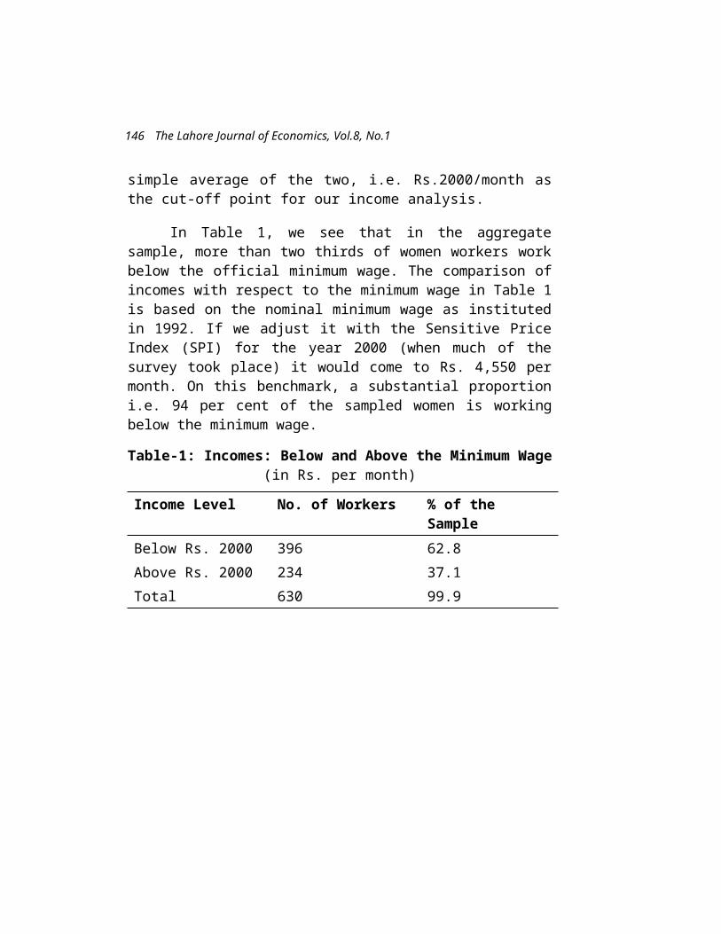
Qais Aslam
transparency in the IMP, the World Bank and the WTO working, as well as reforms in the IMP and the global financial system.
Joseph Stiglitz concludes, “It’s not easy to change how things are done. Bureaucracies, like people, fa11 into habits, and adapting to change can be painful. But the international institutions must undertake the perhaps painful changes that will enable them to play the role they should be playing to make globalisation work, and work not just for the well off and the industrialized countries, but also for the poor and the developing nations”.
Joseph Stiglitz in his book highlights the following points:
1. Globalisation and the introduction of a market economy have not produced the promised results. Not only in trade liberalisation but also in every other aspect of globalisation even seemingly well-intentioned efforts have often backfired. The policies that have been imposed on developing countries in the process of globalisation need to be radically rethought.
2. Abandoning globalisation is neither feasible nor desirable. Globalisation can be reshaped to realize its potential for good and the international economic institutions can be reshaped in ways that will help ensure that this is accomplished.
3. Stiglitz advocates a globalisation with a more human face. Caring about the environment, making sure the poor have a say in decisions that affect them, promoting democracy and fair trade are necessary if the potential benefits of globalisation are to be achieved.
4. Weak governments and too-intrusive governments have both hurt stability and growth. Therefore he advocates a strong, democratic and economic process to stabilise the socio-economic process in
183

The Lahore Journal of Economics, Vol.8, No.1
each country. The political, social, and historical context of each country differs. One attribute of the success cases is that policies of change are ‘homegrown’, designed by the people within each country, sensitive to the needs and concerns of their countries.
5. About rules of global interaction he thinks that these must be seen to be fair and just, must pay due attention to the poor as wel1 as the powerful, must reflect a basic sense of decency and social justice. And these rules have to be arrived at through democratic processes.
6. The IMP has made mistakes in all the areas it has been involved in. Privatisation needs to be part of a more comprehensive programme, which has appropriate legal structures and market institutions, but the ‘adjustment policies’ in country after country forced cutbacks in education and health and that is the real cause of discontent towards globalisation in the developing world.
7. There are alternatives to IMP-style programmes, other programmes that may involve a reasonable level of sacrifice, which are not based on market fundamentalism, programmes that have had positive outcomes. The time has come to ‘grade’ the international economic institution’s performance and to look at some of those programmes.
The economic policies for humanising globalisation suggested in the book are well placed and in line with the real purpose and aims of the globalisation process - poverty reduction; safety nets, environmental protection, transparency of institutions and governments and good governance in developing as wel1 as developed countries with adequate role for the governments to install stable institutions while leaving economic growth to the forces of the tree market. What is new is the suggestion of an international order that can regulate the working and
184

Qais Aslam
policy making of international economic organisations and the exploitative policies of the governments, especially of the governments of the developed countries of the North while negotiating trade agreements and treaties with their less developed partners from the South.
A book is worth reading and keeping in which the author as an ‘insider’ to the events of globalisation and the international institutions bravely picks up issues that only the ‘outsiders’ were previously pointing to. But in the end he does not recommend scrapping of the IMF and World Bank while pointing out that they have miserably failed, but only recommending reforms in these economic institutions which would surely fall on deaf ears of the managers of these institutions and subsequently the managers of the global financial and development system financed through and dictated by the policymakers in these very international institutions.
Apart from its economic and political importance, this book is pleasant to read and all statements are followed by facts that although not documented by footnotes, are explained in a way that those that have been criticised would find hard to refute. More so that Stiglitz in his book is not attacking globalisation itself, just the way the globalisation process has been held hostage to the dictates and highhanded one-sidedness of the bureaucrats in the international organisations and the financial and commercial lobbies in the industrially developed nations. This against the interests of the very poor in the developing world, who should have had gained by this process but have seemingly lost out because of it.
Government College University Qais AslamLahore
185

Notes For Authors1. Manuscripts of research articles, research notes, review
articles, comments, rejoinders and book reviews - in English only - should be sent in duplicate together with floppy in MS - Word to the Editor, The Lahore Journal of Economics, 105, C-2, Gulberg-III, Lahore-54660. Each request for a book review in the journal must be accompanied by one copy of the book concerned.
2. Manuscripts will be accepted for consideration on the understanding that they are original contributions to the existing knowledge in the fields of Economics, Banking, Current Affairs, Finance, Sociology, and Economic History.
3. Each manuscript should be typed and should carry a margin of an inch and a half on the left-hand side of the typed page.
4. The first page of the manuscript should have the title of the paper, the name(s) of author(s) and a footnote giving the current affiliation of the author(s) and any acknowledgments.
5. Authors are requested to use English spellings and not American. For example, organisation and not organization; labour and not labor.
6. Detailed derivations of any main mathematical results reported in the text should be submitted separately along with the articles.
7. Tables for the main text and each of its appendices should be numbered serially and separately. The title of each table should be clearly expressive of the contents. The source of the table should be given in a footnote immediately below the line at the bottom of the table.
8. Footnotes should be numbered consecutively.
9. All references used in the text should be listed in alphabetical order of the authors’ surnames at the end of the text. References in the text should include the name(s) of author(s) with the year of publication in parentheses. Attempt should be made to conform to the style of the

Journal. Further information on questions of style may be obtained from the Co-Editor, The Lahore Journal of Economics, Pakistan.
10. Each author will receive two copies of The Lahore Journal of Economics with the compliments of the LJE.
11. Book Reviews should give a description of the contents of the volume and a critical evaluation of the book. It should not exceed 5 or 6 typewritten pages.

THE LAHORE JOURNALOF
ECONOMICSLahore School of Economics
105-C-2, GULBERG III LAHORE, PAKISTAN. TEL: 5876065 Ext. 153 FAX: 5714936
SUBSCRIPTION FOR PUBLICATIONS
1. Kindly enter a subscription for the following publication of the Lahore School of Economics:
PublicationYearly subscription Yearly subscription Period Total
(within Pakistan) (outside Pakistan) (No. of years)Payment
1. The Lahore Journal Rs. 600.00 US $ 50 …......... ………….
of Economics2. The subscription is to be in the following name and
address:
Name: ----------------------------------------
Address: ----------------------------------------
----------------------------------------
----------------------------------------
3. A crossed cheque/demand draft for the sum of Pakistan Rupees/US $________ is enclosed made out in the name of The Lahore School of Economics to cover the above subscription.
4. Please address your order to: Nina Gera, Publications, Lahore School of Economics, 105-C-2, Gulberg III, Lahore 54660, Pakistan.

Signature:------------------------------------
Name:-----------------------------------------
Date:------------------------------------------

The Lahore School of Economics
The Lahore School of Economics (established 1993) is one of Pakistan’s leading centres of learning for teaching and research in economics, finance and business administration. The Lahore School of Economics’ objectives include: (i). The training of young Pakistanis as professional economists, finance managers, accountants, financial analysts, bankers and business executives, and (ii). Undertaking research in economics, management, finance and banking to further deepen understanding of major economic facts, issues and policies.
The Lahore School was granted a Charter in January, 1997 by an Act of the Provincial Assembly of the Punjab: The Lahore School of Economics Act 1997 (Act II of 1997). The Charter vests the powers of an independent degree granting institution to The Lahore School.
The Lahore School has both undergraduate and graduate programmes in economics, business information systems and finance. Its postgraduate programme leading to the MPhil degree is administered through the Lahore School’s Centre for Advanced Research in Economics and Business (CAREB). The student body and faculty comprise both national and expatriate Pakistanis and The

Lahore School encourages expatriate Pakistanis to join as students or as faculty.
The Lahore School’s publication programme comprises The Lahore Journal of Economics (a bi-annual publication), a Seminar Paper Series and a Text Book Series. The Programme encourages both in-house and external contributors.
For further information, please call (Pakistan 92-42-) 5714936 or 5874385 or E Mail: [email protected] or Web page: www.lahoreschoolofeconomics.edu.pk
Printed by ALBERUNI DTP