bongjunkim - interactive audio lab
TRANSCRIPT

Sound object labeling
EECS 352 Machine perception of Music and AudioBongjun KimWinter, 2019
1

Sound object labeling
Dog barking
2
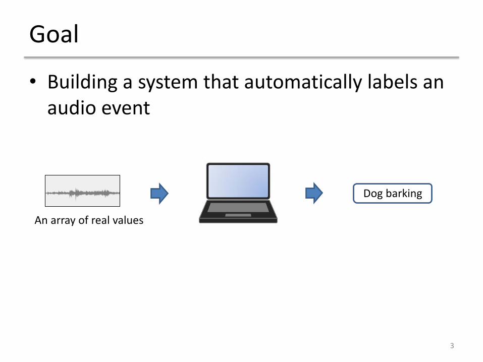
Goal
• Building a system that automatically labels an audio event
An array of real values
3
Dog barking
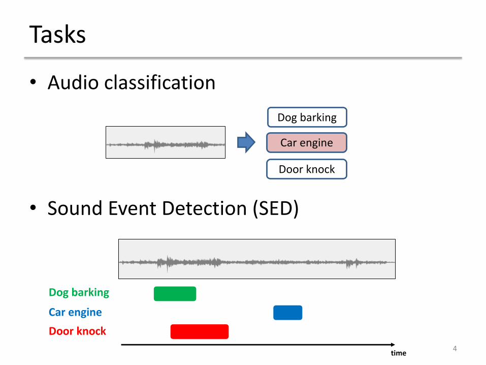
Tasks
• Audio classificationDog barking
Car engine
Door knock
• Sound Event Detection (SED)
Car engineDoor knock
Dog barking
time 4
MACHINE LEARNING: CLASSIFICATION
5

Supervised learning from data
Car engine
!"( )
#
ℎ (!) ≈ "(!)Find a hypothesis function ℎ such thatOn the training data D = {< %1, &1 >,… < %n, &n >}
# = "(!)è
6
Car engineClassification model
! = {%1, %2, …, %n} & = {&1, &2, … &n}
Car engineCar engineDog barking
ℎ ( )
Training input Ground truth labels
Function we want to learn(Target function)
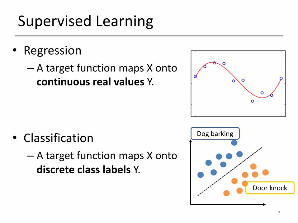
Supervised Learning
• Regression– A target function maps X onto
continuous real values Y.
• Classification– A target function maps X onto
discrete class labels Y.
Dog barking
Door knock
7

Overview of general classification tasks
Input data Label
“Cat image”
“Piano sound”
Classifier
- Decision Tree
- Nearest Neighbor
- Neural Networks
8
Feature representation
!⃗ = <a1, a2, …, an >A vector of numbers
…that represent attributes of the example, like fundamental frequency, or amplitude.
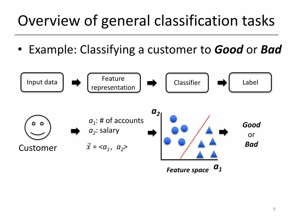
Overview of general classification tasks
• Example: Classifying a customer to Good or Bad
Customer
Input data
!⃗ = <a1 , a2>
a1: # of accountsa2: salary
Feature representation
a1
a2
Feature space
Classifier
Goodor
Bad
Label
9

Different Classifiers
• Different classifications need different classifiers.
RightLeft
RedBlue
Bryan Pardo, EECS 352 Spring 2012 10

Feature selection is important
• How things cluster depend on what you are measuring.
Bad feature representations Good feature representations
11

Which of these go together?
12

Which of these go together?
13Body size
Length of legs

Which of these go together?
14# of legs
Furry

Nearest Neighbor (NN) Classifier
• When you see a new instance ! to classify, find the most similar training example and assign its label to the instance.
• How do you tell what things are similar?1. Extract proper features.2. Measure distance / similarity in the feature space.
15

Nearest Neighbor (NN) Classifier
X
The nearest neighbor
Feature 2
Feature 1
: Class-1 : Class-2
X is classified into class-1
A new instance to classify
16

Nearest Neighbor (NN) Classifier
X
The nearest neighbor
Feature 2
Feature 1
: Class-1 : Class-2
X is classified into class-2
A new instance to classify
17

Nearest Neighbor (NN) Classifier
Feature 2
Feature 1
: Class-1 : Class-2
18
The decision boundary

How do we measure distance?
• Euclidian distance– what people intuitively think of as �distance�
Dimension 1: x
Dim
ensio
n 2:
y
22 )()(),( yyxx babaBAd -+-=
19

Lp norms
• Lp norms are all special cases of this function:
20
L1 norms = Manhattan Distance: p=1
L2 norms = Euclidean Distance: p=2

Cosine Similarity • Measure of similarity between two vectors– Range from -1 (opposite) to 1 (same)– Cosine distance = 1 – cosine similarity
• Cosine similarity between vector A and B:
21
! " # = &!'#'(
')*! # = &!'+
(
')*&#'+(
')*
,-. !, # = ! " #! #

Feature Scaling• Different scales of features can mislead
distance measure.E.g., Measuring distance between humans- Feature 1: Height (0-7 feet)- Feature 2: weight (0-150 kg)
(5.5 feet, 70 kg)
(6, 75kg) In this Euclidean space, the second feature dominates the distance, which might lead to mis-clustering.
Scaling each feature such that it ranges from 0 to 1 can help.

K-Nearest Neighbor (KNN) Classifier
• Consider multiple neighbors• Assign most popular label among K nearest
neighbors• More robust to noisy data than NN (k=1)
X
feature 1
feature 2
Considering 4 nearest neighbors (k=4), most popular class is Class-1
: Class-1 : Class-2
23
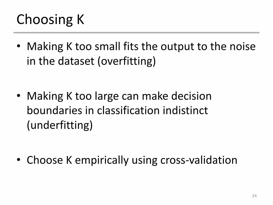
Choosing K
• Making K too small fits the output to the noise in the dataset (overfitting)
• Making K too large can make decision boundaries in classification indistinct (underfitting)
• Choose K empirically using cross-validation
24
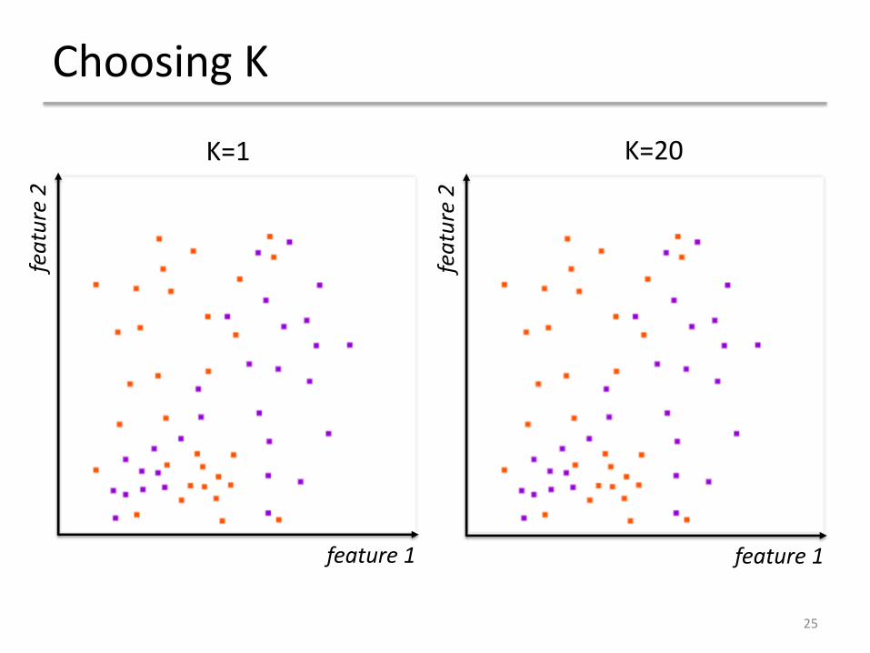
Choosing K
25
feature 1
feat
ure
2
feature 1
feat
ure
2
K=1 K=20

Choosing K
26
feat
ure
2
feature 1
feat
ure
2
K=1 K=20
feature 1Overfitting

Choosing K
27
feat
ure
2
feature 1
feat
ure
2
K=1 K=20
feature 1Overfitting Underfitting

Choosing K
28
K=10
feat
ure
2
feature 1

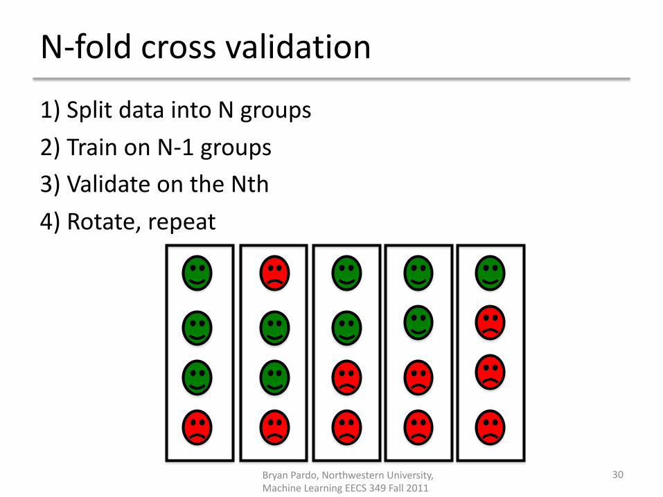
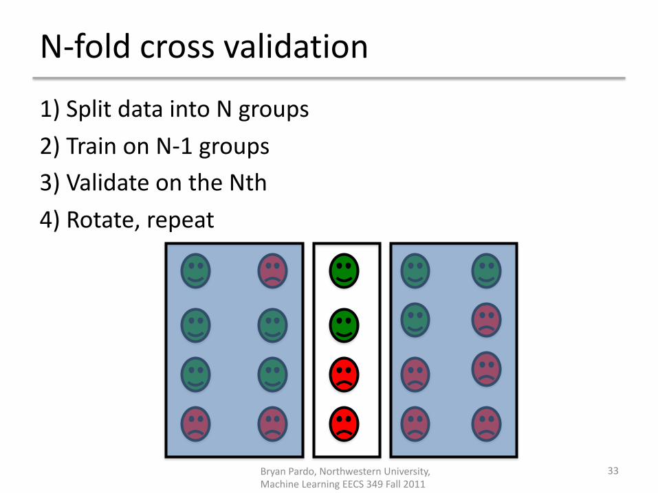
N-fold cross validation1) Split data into N groups2) Train on N-1 groups3) Validate on the Nth4) Rotate, repeat
29Bryan Pardo, Northwestern University, Machine Learning EECS 349 Fall 2011
N-fold cross validation1) Split data into N groups2) Train on N-1 groups3) Validate on the Nth4) Rotate, repeat
30Bryan Pardo, Northwestern University, Machine Learning EECS 349 Fall 2011

N-fold cross validation1) Split data into N groups2) Train on N-1 groups3) Validate on the Nth4) Rotate, repeat
31Bryan Pardo, Northwestern University, Machine Learning EECS 349 Fall 2011

N-fold cross validation1) Split data into N groups2) Train on N-1 groups3) Validate on the Nth4) Rotate, repeat
32Bryan Pardo, Northwestern University, Machine Learning EECS 349 Fall 2011
N-fold cross validation1) Split data into N groups2) Train on N-1 groups3) Validate on the Nth4) Rotate, repeat
33Bryan Pardo, Northwestern University, Machine Learning EECS 349 Fall 2011

Evaluation: Classification accuracy
• Evaluation on a dataset that has NOT been used in model building.
• Classification accuracy– # of correct classifications / total # of examples
• Example: comparing two classifiers– Classifier 1: 80% of accuracy– Classifier2: 78% of accuracy– Which one would you pick for your system?
• Classification accuracy might hide the details of the performance of your model.
34
Evaluation: Confusion matrix
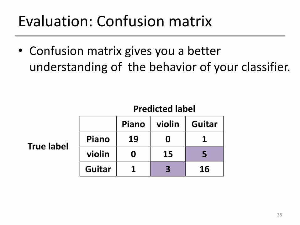
• Confusion matrix gives you a better understanding of the behavior of your classifier.
35
Piano violin GuitarPiano 19 0 1violin 0 15 5Guitar 1 3 16
True label
Predicted label

Evaluation: Confusion matrix
• Confusion matrix gives you a better understanding of the behavior of your classifier.
36
Piano violin GuitarPiano 19 0 1violin 0 15 5Guitar 1 3 16Tr
ue la
bel
Predicted label
Piano violin GuitarPiano 20 0 0violin 7 11 2Guitar 1 0 19Tr
ue la
bel
Predicted label
Classification accuracy: 50/60 = 83%
Classification accuracy: 50/60 = 83%

Now that we know..
• How to build a KNN classifier • How to evaluate it
• We need to learn how to extract feature representations from audio input to build audio classification model.
37
Input data LabelClassifierFeature representation
AUDIO EVENT CLASSIFICATION
38

Audio event classification
Input data Feature representation
Classifier Label
!⃗ = <a1, a2, …, an > “Piano sound”- Nearest Neighbor
We need to convert waveform to feature representations to feed in a classifier.
- We have already learned one of feature representations: Spectrogram
39
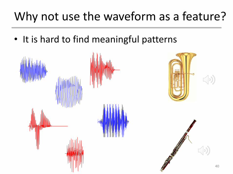
Why not use the waveform as a feature?
• It is hard to find meaningful patterns
40

Why not use the waveform as a feature?
• It is hard to find meaningful patterns
41
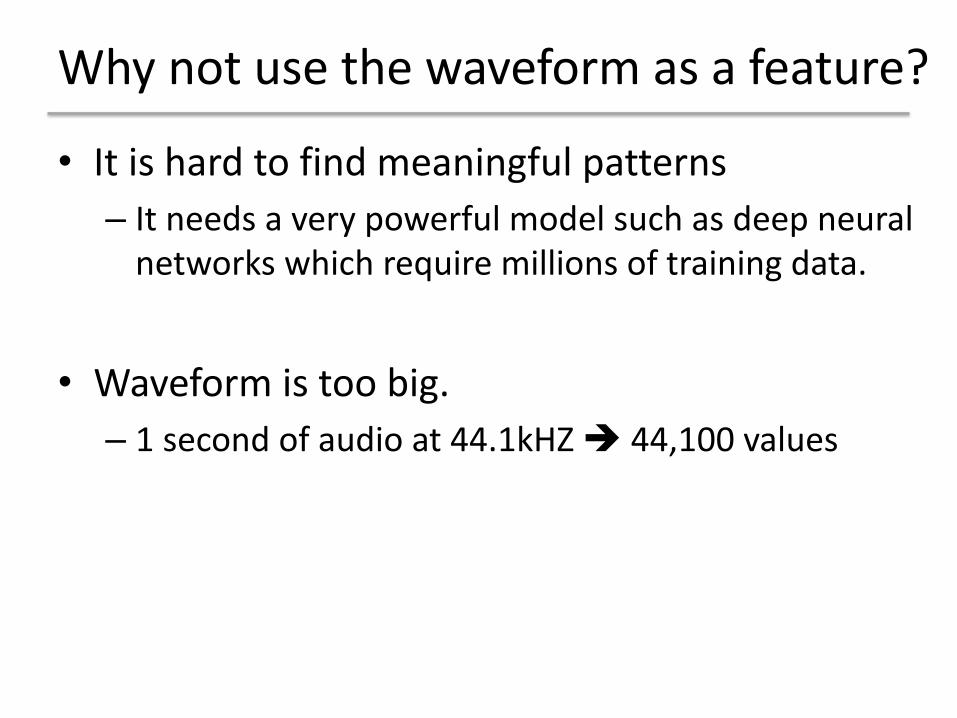
Why not use the waveform as a feature?
• It is hard to find meaningful patterns– It needs a very powerful model such as deep neural
networks which require millions of training data.
• Waveform is too big.– 1 second of audio at 44.1kHZ è 44,100 values

Commonly used audio features
• Zero-crossing rate– Time-domain feature– Rate of sign changes in a signal– Low for harmonic sounds, high for noisy sounds
43* Figure: https://en.wikipedia.org/wiki/Zero_crossing

Commonly used audio features
• Zero-crossing rate
44
Guitar Snare drum White noise

Commonly used audio features
• Spectral centroid– Frequency domain feature– The weighted mean of the frequencies in the signal– Known as a predictor of the “brightness” of a sound
45* figure: https://librosa.github.io/librosa/generated/librosa.feature.spectral_centroid.html

Commonly used audio features
• Spectral centroid
46
Kick drum Snare drum

Automatic drum transcription
47
• Let’s build a drum transcription machine only using spectral centroid features

Automatic drum transcription
48
• Onset detection– librosa.onset.onset_detect
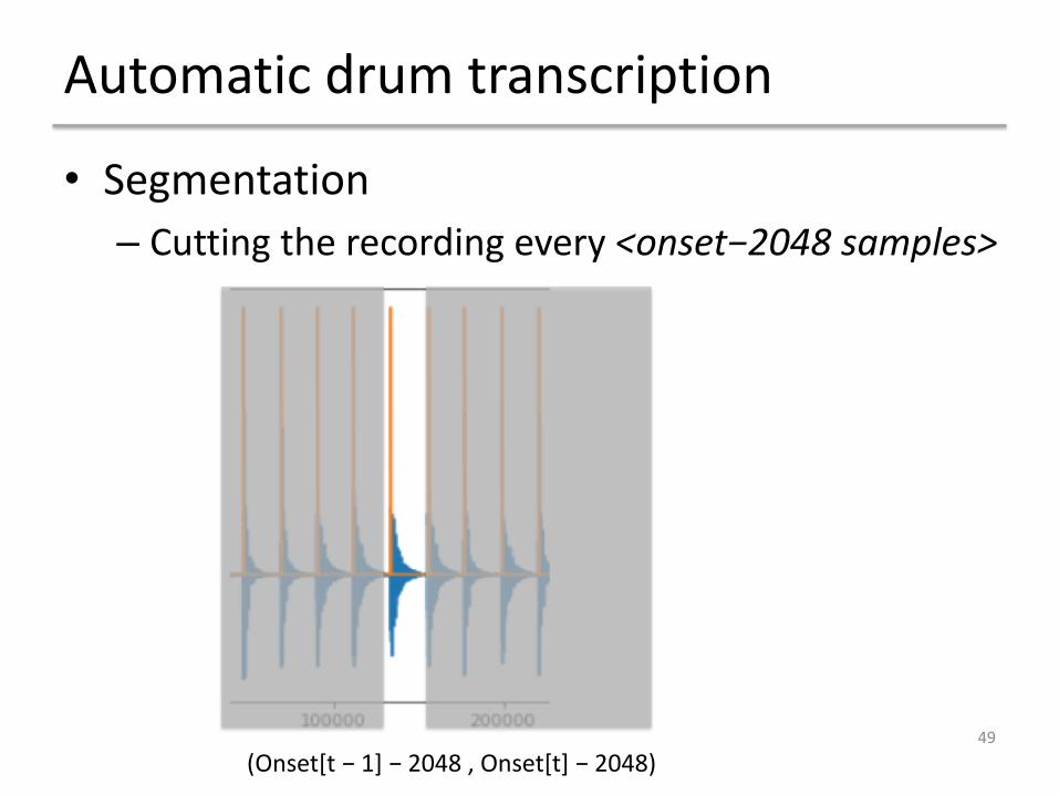
Automatic drum transcription
49
• Segmentation– Cutting the recording every <onset−2048 samples>
(Onset[t − 1] − 2048 , Onset[t] − 2048)

Automatic drum transcription
50
• Extracting spectral centroid from each segment
SnareKick

Automatic drum transcription
51

Automatic drum transcription-2
52
• More challenging example
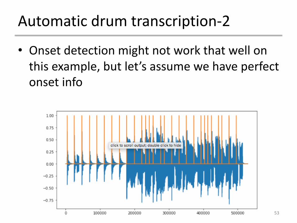
Automatic drum transcription-2
53
• Onset detection might not work that well on this example, but let’s assume we have perfect onset info

Automatic drum transcription-2
54
• Segmentation and feature extraction
• The previous example
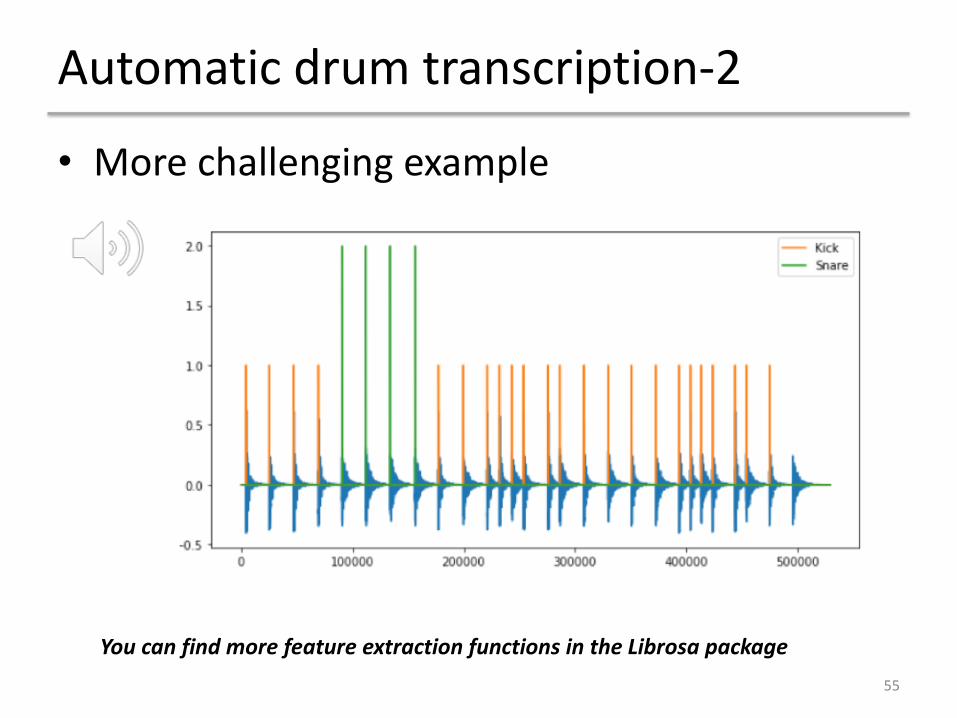
Automatic drum transcription-2
55
• More challenging example
You can find more feature extraction functions in the Librosa package
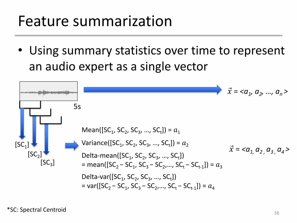
Feature summarization
• Using summary statistics over time to represent
an audio expert as a single vector
56
5s
!⃗ = <a1, a2, …, an >
[SC1]
[SC2][SC3]
Mean([SC1, SC2, SC3, …, SCt]) = #1
!⃗ = <a1, a2 , a3 , a4 >Variance([SC1, SC2, SC3, …, SCt]) = #2
Delta-mean([SC1, SC2, SC3, …, SCt])
= mean([SC2 − SC1, SC3 − SC2,…, SCt − SCt-1]) = #3
Delta-var([SC1, SC2, SC3, …, SCt])
= var([SC2 − SC1, SC3 − SC2,…, SCt − SCt-1]) = #4
*SC: Spectral Centroid

Feature summarization
• Example for multi dimensional features
57
…
Summarizeover time
Mean Variance
Concatenate

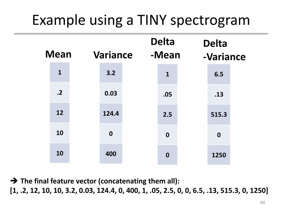
Example using a TINY spectrogram
58
1
.2
12
10
10
Mean3.2
0.03
124.4
0
400
Variance1 0 3 1 5
0 .4 0 .4 .2
0 29 1 20 10
10 10 10 10 10
0 0 0 50 0
frequ
ency
Time
Spectrogram

Example using a TINY spectrogram
1 0 3 1 5
0 .4 0 .4 .2
0 29 1 20 10
10 10 10 10 10
0 0 0 50 0
59
frequ
ency
Time
1
.05
2.5
0
0
Delta-MeanSpectrogram
6.5
.13
515.3
0
1250
-1 3 -2 4
.4 -.4 .4 -.2
29 -28 19 -10
0 0 0 0
0 0 50 -50
DeltaDelta-Variance
frame at (t+1) – frame at t
Example using a TINY spectrogram
60
1
.2
12
10
10
Mean3.2
0.03
124.4
0
400
Variance1
.05
2.5
0
0
Delta-Mean
6.5
.13
515.3
0
1250
Delta-Variance
è The final feature vector (concatenating them all):[1, .2, 12, 10, 10, 3.2, 0.03, 124.4, 0, 400, 1, .05, 2.5, 0, 0, 6.5, .13, 515.3, 0, 1250]

Sound Event Detection by Classification
Car engineDoor knock
Dog barking
time
Context-window
Classification on each context window
61

Challenges• Polyphonic environment, background noise
• Noisy labels
• Using a hierarchical relationship between audio labels
• Weakly labeled training dataset
• A small amount of labeled training dataset
• A large amount of unlabeled training dataset
62

Datasets for sound object labeling
• Urban sound dataset: https://urbansounddataset.weebly.com/
• AudioSet: https://research.google.com/audioset/
• ESC: https://github.com/karoldvl/ESC-50
• DCASE: http://dcase.community/challenge2018/index
• IRMAS: https://www.upf.edu/web/mtg/irmas
• Vocal Imitation Set: https://zenodo.org/record/1340763#.XEtAJs9KiRs
63
EXAMPLE: DOOR KNOCKING / PHONE RINGING CLASSIFICATION
64

Training data
65
Feature extraction and summarization
• Zero-crossing rate and Spectral centroid– window length = 2048, hop length = 1024– Both features are represented as a single number
for each time frame. So we get two feature values for each time frame (2-dimensional space)
– The number of time frames vary with the length of each signal.
• To represent all the signals as the same size of feature vectors, we do summarization.– In this tutorial, I will take mean over frames.
66

Feature extraction and summarization
67
[ZCR, SC][ZCR, SC]
[ZCR, SC]
Mean over time frames[mean(ZCR), mean(SC)]
Now we can map all the signals into 2-dimensional feature space

Plotting them in the feature space
68

Feature scaling
69

Testing examples
70

Plotting test examples
71
Nearest Neighbor classifier would perfectly work in this testing case