Bond UniversityResearch Repository

Role of non parity fundamentals in exchange rate determinationHo, Catherine S F; Ariff, M.

Published in:Malaysian Journal of Economic Studies

Published: 01/06/2008

Document Version:Peer reviewed version

Link to publication in Bond University research repository.

Recommended citation(APA):Ho, C. S. F., & Ariff, M. (2008). Role of non parity fundamentals in exchange rate determination: Australia andthe asia pacific region. Malaysian Journal of Economic Studies, 45(1), 45-69.

General rightsCopyright and moral rights for the publications made accessible in the public portal are retained by the authors and/or other copyright ownersand it is a condition of accessing publications that users recognise and abide by the legal requirements associated with these rights.

For more information, or if you believe that this document breaches copyright, please contact the Bond University research repositorycoordinator.

Download date: 01 May 2020

Bond UniversityePublications@bond

Business papers School of Business

12-1-2008

The role of non-parity fundamentals in exchangerate determination: Australia and the Asia PacificregionMohamed AriffBond University, Mohamed_Ariff@bond.edu.au

Catherine S. F. Ho

This Journal Article is brought to you by the School of Business at ePublications@bond. It has been accepted for inclusion in Business papers by anauthorized administrator of ePublications@bond. For more information, please contact Bond University's Repository Coordinator.

Recommended CitationMohamed Ariff and Catherine S. F. Ho. (2008) "The role of non-parity fundamentals in exchangerate determination: Australia and the Asia Pacific region" Malaysian journal of economic studies, 45(1&2), 1-34.

http://epublications.bond.edu.au/business_pubs/332

C A R F W o r k i n g P a p e r

CARF-F-125

The Role of Non-Parity Fundamentals in Exchange

Rate Determination: Australia and the Asia Pacific Region

M. Ariff

University of Tokyo, Japan, & Bond University, Australia Catherine S. F. Ho

University Technology MARA, Malaysia

August, 2008

CARF is presently supported by AIG, Bank of Tokyo-Mitsubishi UFJ, Ltd., Citigroup, Dai-ichi Mutual Life Insurance Company, Meiji Yasuda Life Insurance Company, Mizuho Financial Group, Inc., Nippon Life Insurance Company, Nomura Holdings, Inc. and Sumitomo Mitsui Banking Corporation (in alphabetical order). This financial support enables us to issue CARF Working Papers.

CARF Working Papers can be downloaded without charge from: http://www.carf.e.u-tokyo.ac.jp/workingpaper/index.cgi

Working Papers are a series of manuscripts in their draft form. They are not intended for circulation or distribution except as indicated by the author. For that reason Working Papers may not be reproduced or distributed without the written consent of the author.

The Role of Non-Parity Fundamentals in Exchange Rate

Determination: Australia and the Asia Pacific Region

M. Ariff and Catherine S. F. Ho*

University of Tokyo, Japan, & Bond University, Australia and *University

Technology MARA, Malaysia;

Mohamed Ariff Professor of Finance, Center for Advance Research in Finance University of Tokyo, Tokyo, Japan and Professor of Finance Department of Finance Bond University, QLD 4229, Australia Email: mariff@bond.edu.au Catherine S.F. Ho Associate Professor Faculty of Business Management University Technology MARA, 40450 Shah Alam, Malaysia. Telephone: (603) 5544-4843 Email: catherine@salam.uitm.edu.my

Working Paper: August, 2008

Acknowledgment: This paper is based on a study that was supported by a

funding to the first author by the University Technology MARA. The study

was completed while both authors were at the Monash University, which also

supported this research by access to the database and funding for research

support to the second author. We thank the anonymous reviewer and the

Editor of the Journal for useful comments while retaining responsibility for

remaining errors.

1

The Role of Non-Parity Fundamentals in Exchange Rate

Determination: Australia and the Asia Pacific Region

Abstract

This paper extends the literature by looking at the contribution of non-parity

variables after extracting the impact of parity variables on exchange rates of

Australia and the Asia Pacific countries. Exchange rates are examined using

high- and low-frequency multi-country panel time series data for a group of

trade-related nations in the Asia Pacific, including Japan. Our findings

suggest that exchange rate is affected by growth rate, and trade and capital

flows: other less significant variables include sovereign debt; balance of

payments; money supply; and trade openness. It also confirms that interest rate

has significant effect on exchange rates while price effect is not significant in

short run regressions. These key findings are robust across different time

intervals, thus showing new findings on the exchange rate dynamics consistent

with theories.

Keywords: exchange rates, parity theorems, trade and capital flows, foreign debt and reserves, growth, monetary and fiscal policy. JEL classifications: F31; F32; G15

1 Introduction

The motivation of this paper is to present findings on exchange rate behaviour

by including new theory/empirically-verified factors as well as other main

theory-suggested ones to investigate exchange rate determination in a trade-

related multi-country context using new research tools. One particular

unexplored factor in international finance is the role of capital flows in recent

decades in the determination of exchange rates: see Harvey (2001). There is a

need to go beyond the traditional price and interest parity factors employed to

study exchange rates of small to medium-size economies. Secondly, after

2

much effort at studying bilateral (two-country) exchange rate determination,

which has yet provided consistent findings in a vast literature of this ilk, new

approach using multi-country framework and improved research design is

needed to understand exchange rate equilibrium. That is what this paper does.

Researchers have expressed increasing frustration over their failures to

explain exchange rate movements (Dornbusch, 1987; MacDonald and Taylor,

1992). With rapid growth in trade and capital flows across national boundaries,

newer key factors are becoming noticed as affecting the value of foreign

currency (Harvey, 2001). These factors are many and include current account

deterioration, excessive foreign debt accumulation, capital flows, foreign

currency reserves and fiscal imbalances. Additional factors that are viewed

and verified in some studies as affecting exchange rate are: economic growth;

exchange rate regimes; and uncontrolled monetary expansion.

This study extends exchange literature by looking at the contributions

of non-parity variables after extracting the impact of parity variables in a first

step: for this we use a two-step regression popularised in the 1990s, and

widely used in Finance. The resulting findings provide improved

understanding of the dynamics of how exchange rates are determined in trade-

related multi-country context by using control factors beyond the traditional

parity conditions. We include countries in a trade-related group if that country

has a majority of trade with the other countries in the grouping.1 We also

provide a single country study of Australia as well.

For the multi-country Asia Pacific region as a whole, we find that the

interest rate parity holds well and this study concludes that increases in

nominal interest rates lead to downward movements in exchange rates, that is

exchange rate improves as Fisher Effect kicks in. Faster economic growth rate

3

in the region significantly facilitates the strengthening of currency values. In

addition, monetary expansions are positively related to domestic exchange

rates and this might be a reflection of faster growth rates driving monetary

expansion. From the separate findings for Australia as a comparison with a

developed country in the region, economic growth rate is the major

determinant of exchange rate movements; accumulation of international

reserves and the domestic monetary stance are also important factors in the

shorter term.

The remainder of this paper is divided into five sections. The next

section contains a brief overview of the current literature, which assisted in

identifying fundamentals relevant to this study. Section three illustrates the

methodology involved, followed by report of significant findings and

robustness testing in section four and five respectively. This paper ends with a

conclusion in section six.

2 Literature on Exchange Rate Determination

The currency exchange market is the world’s largest market in terms of daily

trading volume - in excess of US$ 2.3 trillion in 2007 - no comparison to even

the world’s combined bond or stock markets.2 The imports and exports of

goods and services, coupled with international capital flows could account for

only part of this huge currency transaction: speculative trades in currency is a

major part of this transaction. The primary function of the foreign exchange

market is to facilitate international trade and investment as well as to permit

transfers of purchasing power denominated in one currency to another.

The two parity theorems of exchange rates include the Purchasing

Power Parity (PPP of Cassel, 1918) as well as the Interest Rate Parity (IRP of

Fisher, 1930). These theorems have been extensively tested by renowned

4

scholars all over the world. Interest in currency behaviour is rekindled because

of the incompleteness of our knowledge on exchange rate determination in the

face of periodic currency crises, and by the availability of newer statistical

tools, as well as the accumulation of data over lengthy periods.

2.1 Purchasing Power Parity

PPP has been viewed by many as a basis for international comparison

of income and expenditures, an equilibrium condition; and efficient arbitrage

condition in goods as a theory of exchange rate determination. PPP established

a common ground for cross-country comparison by linking currencies of

different countries to price levels - or more precisely, price differences across

countries - as the base. The underlying theory is based on a simple goods

market arbitrage argument: ignoring tariffs, transportation costs, and assuming

common goods consumed that should ensure identical prices across countries,

under the law of one price. While this notion appears simple enough,

specifying comparative prices between two countries in the short run is

difficult. This has led to a majority of empirical literature failing to verify that

PPP holds.3

The relative version of PPP suggests that if a country’s inflation rate is

relatively higher than its trading partner’s, that country will find its currency

value falling in proportion to its relative price level increases. The exchange

rate E adjusts by k as a function of dP domestic prices and fP foreign prices.

⎟⎟⎠

⎞⎜⎜⎝

⎛= f

d

PPkE (1)

Taking the log on both sides to study changes in exchange rates, arriving at a

testable proposition, where j represents country, t represents time period, P

represents prices, d domestic and f foreign as stated below:

5

ln lnd

tjt j j jtf

t j

PE a bP

μ⎛ ⎞

= + +⎜ ⎟⎝ ⎠

(2)

In order to allow for constant price differential between baskets, the bulk of

empirical tests focused on testing relative consumption based PPP which

require that changes in the relative price levels between countries be offset by

changes in their bilateral exchange rates.

Evidence on short run PPP holding is lacking. It seems that the theory

of PPP had failed to hold.4 The apparent lack of evidence even under mostly

the current floating regimes provides researchers opportunity to revisit this

theme. It is also the same urge that led to the development of the sticky price

model of Dornbusch (1976). In the last two decades, after a number of studies

using unit root tests, researchers have still failed to reject the null hypothesis

of the random walk.5 Froot and Rogoff (1994) concluded that PPP is not a

short-run relationship: this is the basis of our research design to be explained

later to use different time intervals. Prices do not offset exchange rate swings

on a monthly or even annual basis. Frankel and Rose (1996a) examined PPP

using a panel data set of 150 countries over forty-five years and confirmed that

PPP holds and their estimate implied a half-life of PPP deviations of four

years, i.e. it is long term.

2.2 Interest Rate Parity

Interest rate parity, IRP, is the law of one price in the asset market for

securities.6 In theory, the foreign exchange market should be in equilibrium

when deposits of all currencies offer the same rate of return. A rise in interest

rates will attract more investment into the country resulting in an appreciation

of the currency in the short run and exchange rates should fall in the long run

to restore equilibrium. According to the uncovered interest rate parity, the

6

ratio of changes in exchange rate E, within a time period t, is a function of

domestic interest rate , and foreign interest rate . di fi

1 11

dt t

ft t

EE i

+ ⎛ ⎞+= ⎜ +⎝ ⎠

i⎟ (3)

While PPP implies that exchange rates will adjust to changes in

inflation differentials; International Fisher Effect (IFE) implies that relative

interest rate differentials will give rise to similar final results in exchange rates.

The ability of exchange rate markets to anticipate interest differentials is

supported by several empirical studies that indicated the long run tendency for

these differentials to offset exchange rate changes.7

2.3 Non-Parity Variables

Some researchers point out, over the last two decades, that there are

other variables which are correlated with exchange rate movements.8 These

variables could shed fresh light, and assist in identifying other-than-parity

explanations for understanding exchange rate behaviour. Despite the fact that

parity explanations have gained a centre stage up until about the 1980s for

exchange rate behaviour research, recent years have witnessed interests in

other explanations, given the conflicting empirical evidence on parity theories.

The evidence in theory and in empirical studies on these non-parity variables

are systematically examined here.

2.3.1 Current and Capital Account Deterioration

Studies of financial crises in Latin America and East Asia have been

motivated by an interest in the roles of banking, and balance of payments. The

trade and capital balances are known to be most sensitive to exchange rate

changes. For countries affected by the 1997/8 Asian financial crisis, the

7

reversal of capital flows, and current account deficits (together with high

foreign debt) have been suggested as common factors surrounding that crisis.9

Karfakis and Kim (1995) using Australian exchange rate data found

that unexpected current account deficit is associated with a depreciation of

exchange rates and a rise in interest rates. Evidence that current account

deficits reduced domestic wealth and may thus lead to overshooting of the

exchange rates thus a fall in the real value of the currency were also reported

by Obstfeld and Rogoff (1995a), Engel and Flood (1985), and Dornbusch and

Fisher (1980). There has also been a surge in international capital flows into

developing countries in the recent decades. 10 These capital flows affect

domestic output, real exchange rates, capital and current account balances for

years thereafter.11

Portfolio investment has also increased in recent years due to greater

access to capital markets via newer regulations, reduced capital controls and

the overall globalisation of financial services.12 Calvo, Izquierdo and Talvi

(2003) blamed the fall of Argentina's currency programme on their country's

vulnerability to sudden stops in capital flows. A recent study by Kim (2000)

on four countries that faced currency crises found that reversal of capital flows

as well as current account deficits are significantly related to currency crises in

these countries. 13 Rivera-Batiz and Rivera-Batiz (2001) concluded that

explosion of capital flows resulted in higher interest rates and depreciation of

exchange rates in the long run.

2.3.2 Loss of International Reserves and Excessive Foreign Currency

Debt

The amount of international reserves held by the central authority is

another factor affecting exchange rate determination.14 Due to the usage of

8

reserves as a means to defend a country’s currency, it provides credibility to

the value of the currency: this suggests that reserves and the type of currency

exchange regime in this case (managed float as a camouflage for trade

advantage) are likely to affect exchange rates.15

Calvo, Leiderman and Reinhart (1994) showed that increase in capital

inflows increase total reserves and real exchange rates of Lain American

countries. Marini and Piersanti’s (2003) study covering Asian countries found

that a rise in current and expected future budget deficits generated

appreciation in exchange rates and a decumulation of external assets, resulting

in a currency crisis when foreign reserves fell to a critical level. Hsiao and

Hsiao (2001) found a unidirectional causality from short-term external

debt/international reserves ratio to exchange rates in Korea. Similar to

Martinez (1999) on Mexico, Frankel and Rose (1996b) studied a large group

of developing countries and found that the level of debt, foreign direct

investment, foreign interest rates, foreign reserves and growth rates affect

exchange rates significantly.

2.3.3 Trade Openness, Slow Growth, Fiscal Imbalances, and Excessive

Monetary Expansion

Globalisation has resulted in domestic financial markets being slowly

more integrated with international financial markets: see Edward and Khan

(1985) and Ariff (1996). Open economies facing capital flows, competitive

interest rates and trade competition from others must lead to a defined

relationship between openness and the rate of growth in some countries.16

Similar to Karras (1999), Papell and Theodoridis’s (1998) study on openness,

exchange rates and prices found stronger evidence of PPP for countries with

9

less exchange rate volatility, and shorter distance from other countries but not

for countries with greater openness to trade.

Among the many models found in the literature to explain long-term

deviations in PPP, the most popular one is from Balassa (1964) and

Samuelson (1964). Both agued that technological progress has historically

been faster in the traded goods sector than in non-traded goods sector and

therefore traded goods productivity bias is more obvious in higher income

countries. Froot and Rogoff (1994) and Rogoff (1999) further showed that

faster growing countries would tend to experience exchange rate appreciation

relative to their slower growing partners when technological changes happen

more often in trading goods sector as a result of intense international

competition. Add to these the following: Canzoneri, Cumby and Diba (1999);

Chinn (2000); Duval (2002); and Cheung, Chinn and Pascual (2003).

MacDonald and Wojcik’s (2003) study on EU accession countries

found that productivity, as well as private and government consumption

significantly affect exchange rate behaviour. In contrast with Edwards and

Savastano (1999), Bailey, Millard and Wells (2001) found that increased

labour productivity in the US resulted in current account deficits that are

financed by large capital inflows, which appreciated the dollar exchange rates.

2.3.4 Exchange Rate Regimes

Since the breakdown of the fixed Bretton Woods system, exchange

volatility has drastically increased to levels that are beyond the explanation of

fundamentals.17 Grilli and Kaminsky (1991) concluded that real exchange

rate behaviour changes substantially across historical periods but not

necessarily across exchange rate regimes. Calvo and Reinhart (2002)

examined thirty-nine countries around the world and found that moderate to

10

large exchange rate fluctuations are very rare in managed float systems. Other

studies that found similar results includes Hasan and Wallace’s (1996), Moosa

and Al-Loughani (2003) and Edwards (2002) who explained that super-fixed

regimes were highly inflexible and inhibited adjustment process.

Hence there is literature support for checking these many non-parity

factors’ role in exchange rate determination.

3 Data, Methodology and Summary Statistics

3.1 Data

The data used relate to exchange rates between individual countries, and the

United States (U.S.) dollar (IFS line rf) as the foreign unit as observed at the

end of observation periods.18 Quarterly bilateral exchange rates for Australia

as well as nine other Asia Pacific countries are from 1974:4 to 2006:1. The

International Financial Statistics (IFS) CD-ROM is the major source for these

data. Price variables include CPI (IFS line 64) and PPI (IFS line 63) of

individual countries; T-Bill and Money market rates (IFS line 60) are used to

arrive at the interest differentials between countries. Changes in exchange

rates, prices and interest differentials are calculated using natural logarithm.

The non-parity current and capital flow variables include: trade

balance (Trade) from imports and exports of goods, and current account

balance (Cur); balance of payments (BOP) from overall balance; capital flows

include both inflows and outflows of foreign direct investment (FDI) and

portfolio investments (PT); and total reserves (TR) as well as foreign debt

(FD). Monetary expansion data is broader money19 (M2) which includes both

money and quasi-money. Growth rate (PROD) is measured by change in

Gross Domestic Product (GDP) per capita. The set of dummy variables

includes exchange regimes which are grouped into three categories: free-float,

11

exchange band/managed, and fixed regime.20 Trade openness is measured by

total trade (TTrade), that is, the sum of total imports and exports, as a

proportion of GDP: this is used to form trade-related groupings. Incomplete

data are sourced from Datastream, World Bank as well as individual country’s

Central Banks and Statistical Departments. The independent variables are

categorised into parity and non-parity variables. 21 A summary of variable

definitions and their expected signs are found in Table 1.

Insert Table 1 here.

The sample in this study includes Australia as an individual country

and a selection of nine countries in the Asia Pacific region: Australia,

Indonesia, Japan, Korea, Malaysia, New Zealand, the Philippines, Singapore

and Thailand. The developed nations include Australia, Japan, New Zealand

and Singapore and the rest are emerging economies with relatively high

growth rates. The reason behind the choice of these nine countries is the high

level of inter-trade between these countries in the same geographical region as

shown in Table 2 and the availability of information with regards to these

nations. We include these countries as each of the countries included has a

majority trade relation, that is import and exports to other countries in the

grouping is well above 50 percent of total trade. We present this as the trade-

relatedness for selecting countries to be included in a regional grouping (and

thus we had five such groups made of 54 countries across the world, although

this paper is on Asian Pacific grouping only). For related data, see Table 2: for

example, Hong Kong has a majority of its trade with the chosen group.

Insert Table 2 here

3.2 Methodology

12

The regression analysis tests the price and interest parity theorems and

then includes other non-parity fundamentals with appropriate tests to check the

robustness and validity of results. The one-step ordinary least squares model

has its limitations and hence a two-step regression is used to explain the

unexplained effects captured in the residuals from the first regression using

parity variables. Ball, Brown and Officer (1990) is a paper collected in Ball,

Brown, Finn and Officer (1990) and they popularized this procedure of

extracting theory suggested variables in the first step regression, and then

taking the residual to test further proposition. This procedure of first running a

regression, and then using the residuals from the first regression as dependent

variable on further independent variables is thus followed. We follow this

procedure as it is well-established in Finance studies. This overcomes the

problem of estimating the parity relations which have significant pair-wise

correlations with non-parity variables. Stepwise parsimonious regression

approach using the well established AIC statistics allows an examination of

each independent variable’s contribution to the model, which will be useful in

selecting a narrower set of variable. The parity and non-parity models include

different tests of the price and interest parities individually as well as jointly in

a multi-country framework.

Combined Price and Interest Parity Test

Investigating both price and interest parities should yield results that

could explain the extent to which parity hypotheses could explain changes in

exchange rates:

' ' '10 1 1* *

1ln ln ln1

tj j j jt

jt jtt jt

E P i eE P i

α α β+⎛ ⎞ +⎛ ⎞ ⎛ ⎞= + + +⎜ ⎟ ⎜ ⎟ ⎜ ⎟+⎝ ⎠ ⎝ ⎠⎝ ⎠ (4)

Non-Parity Models

13

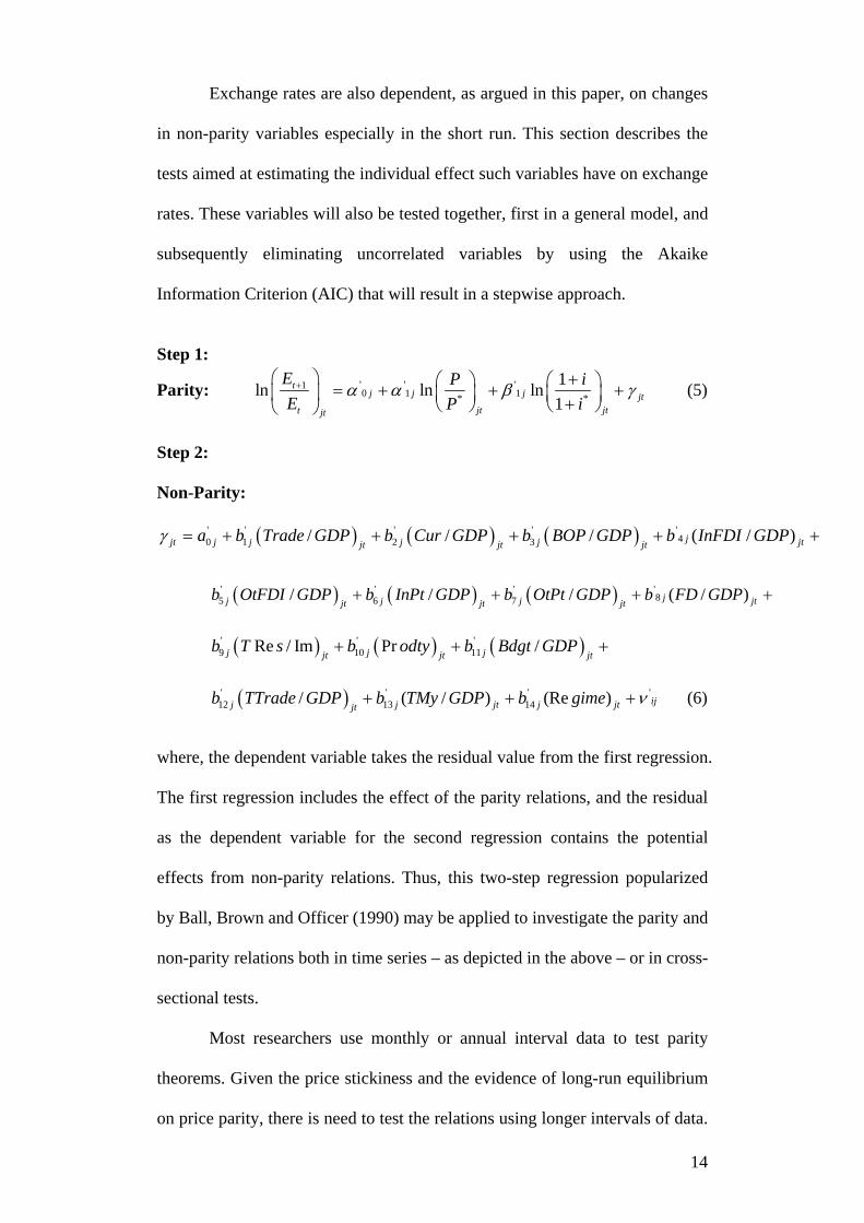
Exchange rates are also dependent, as argued in this paper, on changes

in non-parity variables especially in the short run. This section describes the

tests aimed at estimating the individual effect such variables have on exchange

rates. These variables will also be tested together, first in a general model, and

subsequently eliminating uncorrelated variables by using the Akaike

Information Criterion (AIC) that will result in a stepwise approach.

Step 1:

Parity: ' ' '10 1 1* *

1ln ln ln1

tj j j jt

jt jtt jt

E P iE P i

α α β+⎛ ⎞ +⎛ ⎞ ⎛ ⎞= + + +⎜ ⎟ ⎜ ⎟ ⎜ ⎟+⎝ ⎠ ⎝ ⎠⎝ ⎠γ (5)

Step 2: Non-Parity:

( ) ( ) ( )' ' ' ' '40 1 2 3/ / / ( /jjt j j j j jtjt jt jt

a b Trade GDP b Cur GDP b BOP GDP b InFDI GDPγ = + + + + ) +

( ) ( ) ( )' ' ' '

85 6 7/ / / ( /jj j jjt jt jtb OtFDI GDP b InPt GDP b OtPt GDP b FD GDP+ + + ) jt +

( ) ( ) ( )' ' '

9 10 11Re / Im Pr /j j jjt jt jtb T s b odty b Bdgt GDP+ + +

'jt

( )' ' '

12 13 14/ ( / ) (Re ) ijj j jt jjtb TTrade GDP b TMy GDP b gime ν+ + + (6)

where, the dependent variable takes the residual value from the first regression.

The first regression includes the effect of the parity relations, and the residual

as the dependent variable for the second regression contains the potential

effects from non-parity relations. Thus, this two-step regression popularized

by Ball, Brown and Officer (1990) may be applied to investigate the parity and

non-parity relations both in time series – as depicted in the above – or in cross-

sectional tests.

Most researchers use monthly or annual interval data to test parity

theorems. Given the price stickiness and the evidence of long-run equilibrium

on price parity, there is need to test the relations using longer intervals of data.

14

Therefore, we tested the regression by increasing the interval period and

observing the variables across one-, two-, three- and further years so that the

tests may be conducted over longer interval data to detect the impact of

variables which has long run impacts beyond one or more years. Thus, a 2-

year window means that the variables are observed over a two-year period,

and so forth.

Common problems faced in cross-sectional and time series analysis are

non-normality of variables, non-stationarity of time series data,

multicollinearity among criterion factors, autocorrelation and

heteroscedasticity. The descriptive statistics of the variables are given in the

Appendix 1 to this paper: although not shown in the appendix, the variables

were found to be normally distributed, given the transformation. The impact of

multicollinearity is to reduce any single independent variable’s predictive

power by the extent to which it is associated with the other independent

variables. It can be detected using Variance Inflation Factor (VIF) that shows

how the variance of an estimator is inflated by the presence of

multicollinearity (Hair et al., 1998).22 Variables with larger VIF values or low

tolerance level are excluded: alternatively highly collinear variables may be

joined in some transformation of the series. Our VIF statistics show that

multicollinearity is not present in the regression: see Endnote 21 and the

Appendix 2 to this paper. As may be verified, the VIF statistics are below the

critical values, thus indicating that the multicollinearity is not likely to affect

the test statistics in the regression.

The normality of all the variables will be tested to ensure multivariate

normality and this is further ensured by specifying the variables in natural

logarithms while stationarity of the series will be tested and confirmed by

15

Augmented Dickey-Fuller (ADF) unit root test and the Kwiatkowski, Philips,

Schmidt and Shin (KPSS) Test: see Appendix 3 and also Endnote 21. The

presence of heteroscedasticity is detected by White’s test using Eviews

software: thought the test results are not reported here, we used appropriate

corrections for heteroscedasticity problem. To ensure that the assumption of

constant variance is not violated, the heteroscedasticity and autocorrelation

problems are tested and corrected using the Eviews process for this.

4. Findings

This section reports the quarterly as well as other interval results on both

Australia and the Asia Pacific region. Since the exchange rate used in this

model is against the foreign currency, a negative coefficient corresponds to an

increase in the value of domestic currency and a positive coefficient indicates

otherwise.

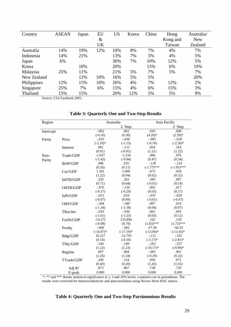
4.1 Short Term - Australia From the quarterly results in Table 3, it is important to note that higher

growth rate stands out clearly as the major determinant of exchange rates in

Australia. This model however, cannot find any indication of the purchasing

power and interest parity in the short term which is consistent with the current

empirical literature. Although statistically insignificant, the coefficient for

trade has the right sign where increase in trade leads to appreciation of the

domestic currency. The coefficient for foreign debt is insignificant and in the

opposite direction to theoretical prediction: it cannot be explained. Capital and

portfolio flows are insignificant but the short run coefficients have the

expected signs. It appears that for a developed country, capital and debt flows

16

do not have a significant impact on its economy and therefore its exchange

rates. That is the short-run story.

Insert Table 3 here.

Total reserves have an insignificant coefficient though the sing is

consistent with theoretical expectation that an increase in reserves raises the

confidence level others have on its currency value. Government’ fiscal budget

is insignificant but of the correct sign. This reflects that fiscal budget condition

does not drive the value of the currency. Monetary policy of the government is

also not significant (t-statistics of 1.22) where excessive monetary expansion

leads to deterioration of currency value. The total trade or trade openness

coefficient is insignificant and the relationship is negative. The sign reflects

that openness to trade resulted in huge imports that send the currency value

falling. The F-probability of 0.000 shows that the model is statistically

significant and that growth rate is the major driving force behind exchange

rate movements. The adjusted R-squared of 0.873 also indicates that more

than 80 per cent of the movement in exchange rates can be explained by this

model.

4.2 Short Term – Asia Pacific

For the region as a whole in Table 3, interest and price parities do not

hold in the short run as these are statistically insignificant in the short run

consistent with current literature. The coefficient for growth rate of -57.30 is

highly statistically significant (t-stats -13.06) with major effect on exchange

rates as well as in the expected direction. Improvement in the balance of

payments leads to an increase in the value of domestic currency in the region;

nonetheless it is only marginally significant with t-statistics of -1.77. It is most

interesting to note that domestic monetary expansion is significant and directly

17

related to the value of the currency. This is not consistent with the monetarists’

model and might be a reflection of rapid growth of the region driving

monetary expansion. The coefficient for foreign debt of 0.162 is statistically

significant (t-statistics 1.83) and shows that increase in sovereign debt

negatively impacting domestic exchange rates. Government’s fiscal budget is

another significant determinant of exchange rates for Asia Pacific countries in

the short term where improvement in the budget balance improves the

exchange rate performance too.

The capital, portfolio flows, and monetary regime are generally

insignificant and this shows that short run quarterly changes in these variables

do not have a strong impact on exchange rates. Total trade of the region is also

significant but is inversely related to exchange rates. This might be explained

by the large amount of imports absorbed into the region when these countries

accumulated wealth through rapid growth which is supported by huge exports

too. Thus trade openness allows these countries to import more productive

technologies and it facilities to enable them to sustain higher and continuous

growth. With adjusted R-squared of 0.738 for a region of nine countries, the

model can explain more than 70 per cent of changes in exchange rates.

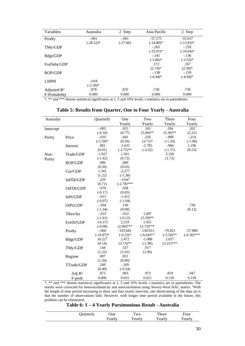
Short Term - Parsimonious Model

The parsimonious model in Table 4 indicates similar findings for the

region and confirms the significance of growth rates and others have on

exchange rates. These results are more reliable. Sensitivity analysis of the tests

is conducted with no substantial differences to the reported results.

Parsimonious model indicates that the coefficients for the five major factors

for the region of Asia Pacific countries are namely (1) growth rates, (2)

balance of payment, (3) budget balance, (4) foreign debt accumulation and (5)

18

total money, continue to be statistically significant which is consistent with

theories and some studies. The other variables are not significant and some of

them have incorrect sign.

Insert Table 4 here

4.3 Longer Term - Australia

The longer term results are shown in Table 5 as a comparison from

short to longer period of time. It is crucial to note that purchasing power parity

is achieved at two years for Australia, which is not only statistically significant

(t-statistics 3.71) and of correct sign. Sample sizes are too small to allow

reliable use of parity fundamentals to predict changes in exchange rates, even

when these fundamentals do determine exchange rates. Further study with

longer time series in the future would obtain more significant results.

Insert Table 5 here

There is without doubt growth rate is the major determinant of

exchange rates in Australia from the results obtained here for quarterly as well

as all subsequent time periods. Fiscal stance is also an important longer term

variable, as fiscal expansion is inversely associated with the movement of

exchange rates and is statistically significant in both one- and three- yearly

regressions. Monetary expansion is becoming more important in the longer

term and the results correspond to theory; it is indirectly related to exchange

rates. It is important to note that exchange rate appreciation of a certain

magnitude always become more worrisome if coupled with excessive

monetary expansion.

The coefficients of foreign debt of 2.219 and 1.951 are significant (t-

statistics 2.90 and 3.73 respectively) and of the correct direction for one, and

two year intervals. This shows that in the longer-term, persistent accumulation

19

of foreign debt decreases the value of the currency when investors lose

confidence in the ability of the country to repay its foreign debt. Moreover,

high foreign debt leads to further deterioration of the economy if accompanied

by high world interest rates.

Non-parity variables which are marginally significant in affecting

exchange rates in the shorter time period also include inflow of foreign direct

and portfolio investments which are positively related to exchange rates in the

one yearly interval. This shows that in the longer term, inflows of investment

increase the value of the Australian currency and likewise for accumulation of

balance in the current account. The R-squared for the all the period intervals

are above 80 per cent and this shows that the models can explain a large

portion of exchange rate movements. In summary, the key driving force

behind the Australian currency is still growth rates in the domestic economy.

Other variables that affect exchange rates include inflow of foreign direct and

portfolio investments, foreign debt accumulation, total trade, and monetary

and fiscal stance of the government.

Parsimonious Model

The results from a parsimonious model given in Table 6 clearly show

that growth rate is the major determinant of exchange rates in Australia. It is

interesting to note that accumulation of reserves and portfolio outflows are

also significant determinants for one and two yearly interval, respectively.

Insert Table 6 here.

4.4 Longer Term - Asia Pacific

Consistent with theoretical position, interest parity theory is

consistently holding in the region as a whole as it is statistically significant in

20

all the yearly intervals in Table 7. Price parity however, is not being explained

in the model here. It might be, since these countries are relatively new with

data of only about thirty years, longer time period and longer series of data

once available in the future, would enable more significant results to be

determined using our intervalling method to control sticky price.

Insert Table 7 here

The coefficient for growth rates, interest rates and total money are

statistically significant in four year interval and are the major forces behind

exchange rates in the region. The growth of countries in this region helps to

explain the increase in currency value throughout the thirty years of the study.

The balance of payment is only a shorter term variable in determining

exchange rates in the region as accumulation of the balance is reflected in an

improvement in exchange rates as predicted. Monetary expansion in the region

is positively related to exchange rates and trade openness is negatively related

to exchange rates as explained in the earlier section.

Although significant only in the shorter term, the coefficient on foreign

debt of 0.262 at four year interval is in the expected direction in the longer

term. Other capital and portfolio flows, current account, and trade flows are

insignificant in affecting exchange rates which is surprising because it is

believed that they are the major reasons for the financial crisis in the region in

1997. This might be due to the insufficient length of time series available from

these countries when some of them only started recording these flows in the

late nineties.

The parsimonious result in Table 8 reinforces the findings from Table

7. Overall, the adjusted R-squared are all above 75 per cent which shows that

21

the models can explain a high proportion of changes in exchange rate in the

region. On top of that, the F- probabilities for the models are very significant.

Insert Table 8 here

5 Robustness Testing

This paper undertakes robustness tests to reaffirm the results. We first remove

statistically insignificant variables from the model to form the parsimonious

model. The results are robust to the removal of these variables, with all

explanatory variables and significance of coefficient persisting. On top of that,

using stepwise approach reconfirms the existing results, as seen above.

We also removed relatively highly correlated variables from the model

(despite the VIF tests) and re-ran the analysis. The results largely persisted.

The outflows of capital and portfolio figures are generally not significant

anyway and when they are removed, the number of observations increases and

adjusted R-squared also increases. Overall, the F- statistics of the models

improved and the models are statistically significant.

6 Conclusion

This study reports new findings, if accepted, may extend the existing currency

literature by considering the extent to which both parity and non-parity

variables influence exchange rates in Australia and also in a region of nine

closely-trading countries in the Asia Pacific. We find that of the non-parity

variables for Australia, three have extensive explanatory power in the models

investigated in this paper: (1) growth rates, (2) foreign debt and (3) fiscal

expansion. Collectively, these variables explain about 80 per cent of the

changes in exchange rates in Australia. The parity variables, on the other hand,

are generally statistically insignificant. Two other non-parity variables which

22

23

are marginal, thus are not significant, include (4) monetary expansion and (5)

inflow of foreign capital.

The major driving forces behind exchange rates in the Asia Pacific

region as a whole are (1) interest rates, (2) growth rates and (3) monetary

expansion. (4) Interest parity is consistently holding in the region for all

intervals of time periods. (5) Price parity however, needs further extension of

data and tests in a future study due to insufficient data available for these

relatively new countries: as mentioned earlier, we could not extend the tests

beyond 4-year intervals, which is too short to reveal the price parity

equilibrium given sticky prices. Other minor non-parity variables that appear

to be statistically borne out are identified: (6) balance of payments, (7)

government’s fiscal balance and trade openness as these factors are not always

significant in all regressions. The explanatory power of models is also large.

It is important to note that different countries face different set of

parity and non-parity variables which are significant in driving their exchange

rates. The results for parity and non-parity variables are robust to alternative

specifications of the model. We believe the tests developed in this study has

led to improved results, and help identify new variables that are related to

exchange rates while the puzzle of short-term versus long term behaviour is

made obvious by applying different interval period. It is to be noted that the

use of different intervalling periods beyond the monthly and quarterly

intervals used by most researchers enabled us to bring in the impact of long-

cycle sticky price effect. Finally, this study ventured to include factors

suggested by theories/empirical reports to identify non-parity variables, which

appear to be very significant contributors to the exchange rate determination.

24

Notes: 1 We grouped 54 countries into 5 trade-related groupings, the Asia pacific countries is one of

the five groupings thus formed.

2 The Economist. April, 2001. Forex is 50 times larger by volume than the equity market as

stated by Euromoney.com. Resnick, Bruce G. Business Horizons, Nov/Dec 89, Vol 32, Issue

6 and updated by others. 3 Empirical work that has led to conflicting empirical findings for PPP includes MacDonald

(1993), Rogoff (1996), Edison, Gragnon and Melick (1997), Cheng (1999) and Bayoumi and

MacDonald (1999). They have all found no clear evidence or at best, very weak relationship

between inflation and exchange rates. 4 Henry and Olekaln’s (2002) study on Australia found little evidence for long run equilibrium

between exchange rate and prices. In a similar view, Adler and Lehman (1983) found that the

deviations from PPP follow a random walk without reverting back to PPP for 43 countries. 5 MacDonald and Ricci (2001), Kuo and Mikkola (2001), Lothian and Taylor (2000), Mark

and Sul (2001), Schnabl and Baur (2002) found considerable evidence for long run relation

and concluded that fundamentals paly a significant role in determining exchange rates. 6 The interest rate theory was first developed by Keynes (1923) and Fisher (1930) through the

introduction of Fisher effect for domestic interest rate theory. 7 Studies that provided evidence include Mark (1995), Chortareas and Driver (2001), Chinn

and Meredith (2002), Hoffman and MacDonald (2003) which found measures of long run

expected changes in exchange rates highly correlated with interest rate differentials. 8 Frankel and Rose (1996b) on current account and government budget deficits; Calvo,

Leiderman and Reinhart (1994) on capital flows, inflation and current account deficits; and

Aizenman and Marion (2002) on reserve and credibility; and many others. 9 It is documented that the recent currency crises were due to vast changes in these variables,

including Kim (2000). 10 Gross foreign direct investment as a percentage of GDP increased more than 100 percent for

Korea, the Philippines and Indonesia for the period 1990-2001.Net private capital flows into

six developing regions in the world totalled US$167.976 millions in 2001. Source: 2003

World Development Indicators, database, World Bank, 13 April 2003. 11 Studies on capital flows that affect output, exchange rates and balance of payments include

Kim (2000) and Calvo and Reinhart (1999). 12 Portfolio investment inflows have increased from RM19,346 millions in 1991 to a peak of

RM238,454 millions in 1994 for Malaysia. Source: Bank Negara Malaysia and Department of

Statistics, Malaysia. Portfolio investment averaged US102 billion for 1995-96 and US26

billion for 1997-2000 according to World Economic Outlook, 2003, IMF. 13 Using annual data for 21 OECD countries, Krol (1996) found that capital flows have

significant effect on current accounts as well as exchange rates and this is reinforced by Kim

(2000).

25

14 Korea’s usable reserve fell from US$28 billion to a mere US$6 billion when their currency

went on a free fall in December 1997: Aizerman and Marion (2002). Brazil’s reserves fell

from US$75 billion to less than half of that before the currency collapsed in 1998: Dornbusch

and Fisher (2003). 15 Total external debt for six developing regions in the world according to World Bank

classification amounted to US$2,332,621 millions for 2001. Source: 2003 World Development

Indicators, World Bank. 16 Karras and Song (1996) investigated 24 OECD countries for thirty years and found positive

relationship between output volatility, economy’s trade openness and exchange rate flexibility. 17 Reviewing the US experience with flexible exchange rates, Dornbusch (1987b) found that

changes in exchange rates in the last fifteen years are inconsistent with any explanations in

theory and may not be related to fundamentals. 18 These exchange rate quotations can be expressed in either a unit of foreign currency (Direct

quote) or a local unit expressed in foreign equivalent (Indirect quote). A direct exchange rate

quotation gives the home currency price of in terms of foreign currency whereas the indirect

quote gives the one unit home currency equivalent in foreign currency. They are actually the

reciprocal of each other. In order to avoid confusion, direct quotations are used, as is the

practice in the literature, in this study unless stated otherwise. 19 IFS defined money as the sum of currency outside deposit money banks and demand

deposits, and quasi money as the sum of time, savings and foreign currency deposits of

resident sector. 20 Exchange regimes are according to Reinhart and Rogoff (2002). 21 In order to minimize multicollinearity effects, all parity variables were transformed as first

difference and specified in the models as natural logarithm. Further investigation of the

variables indicated that there is no significant correlation among the independent variables

using VIF tests. 22 These test results are shown in this paper in the Appendix 2 on more than the variables

included in this study: we did the tests with the methods described in this paper and other

methods used to study the other four regions.

References: Adler, M., & Lehman, B. (1983). Deviations From Purchasing Power Parity in the Long Run.

Journal of Finance, 38(5): 1471-1487. Aizenman, J., & Marion, N. (2002). Reserve Uncertainty and The Supply of International

Credit. Journal of Money, Credit, and Banking, 34(3): 631-649. Ariff, M. (1996). Effects of Financial Liberalization on Four Southeast Asian Financial

Markets, 1973-94. ASEAN Economic Bulletin, 12(3): 325-338. Ariff, M., & Khalid, A. M. (2000). Liberalization, Growth and the Asian Financial Crisis:

Lessons for Developing and Transitional Economies in Asia. Cheltenham, UK; Northampton, MA, USA: Edward Elgar.

Bailey, A., Millard, S., & Wells, S. (2001). Capital Flow and Exchange Rates. Bank of England Quarterly Bulletin, London, 41(3): 310-318.

Balassa, B. (1964). The Purchasing-Power Parity Doctrine: A Reappraisal. The Journal of Political Economy, 72(6): 584-596.

26

Ball, R., Brown, P., Finn, F. J., & Officer, R. R. (1980). Share Markets and Portfolio Theory:

Readings and Australian Evidence. St Lucia, Qld: University of Queensland Press. Bayoumi, T., & MacDonald, R. (1999). Deviations of Exchange Rates from Purchasing Power

Parity: A Story Featuring Two Monetary Unions. IMF Staff Papers, 46(1), 89-102. Calvo, G. A., & Reinhart, C. M. (1999). Capital Flow Reversals, The Exchange Rate Debate

and Dollarization. Finance & Development, 36(3): 13-15. Calvo, G. A., & Reinhart, C. M. (2002). Fear of Floating. The Quarterly Journal of

Economics, 117(2): 379-408. Calvo, G. A., Izquierdo, A., & Talvi, E. (2003). Sudden Stops, The Real Exchange Rate, and

Fiscal Sustainability: Argentina's Lessons. National Bureau of Economic Research Working Paper, 9828.

Calvo, G. A., Leiderman, L., & Reinhart, C. M. (1994). The Capital Inflow Problem: Concepts and Issues. Contemporary Economic Policy, 12(3): 54-60.

Canzoneri, M. B., Cumby, R. E., & Diba, B. (1999). Relative Labour Productivity and The Real Exchange Rate in the Long Run: Evidence for a Panel of OECD Countries. Journal of International Economics, 47(2): 245-266.

Cassel, G. (1918). Abnormal Deviations in International Exchanges. The Economic Journal, 28(112), 413-415.

Cheng, B. S. (1999). Beyond the Purchasing Power Parity: Testing for Cointegration and Causality Between Exchange Rates, Prices and Interest Rates. Journal of International Money and Finance, 18, 911-924.

Cheung, Y.-W., Chinn, M. D., & Pascual, A. G. (2003). What Do We Know About Recent Exchange Rate Models? In-Sample Fit and Out-of Sample Performance Evaluated. CESifo Working Paper, 902.

Chinn, M. D. (2000). The Usual Suspects? Productivity and Demand Shocks and Asia-Pacific Real Exchange Rates. Review of International Economics, 8(1): 20-43.

Chinn, M. D., & Meredith, G. (2002). Testing Uncovered Interest Parity at Short and Long Horizons During the Post-Bretton Woods Era. National Bureau of Economic Research Working Paper.

Chortareas, G. E., & Driver, R. L. (2001). PPP and the Real Exchange Rate-Real Interest Rate Differential Puzzle Revisited: Evidence from Non-Stationary Panel Data. The Bank of England Working Paper Series.

Demarmels, R., & Fischer, A. M. (2003). Understanding Reserve Volatility in Emerging Markets: A Look at the Long-Run. Emerging Markets Review, 4: 145-164.

Dickey, D. A., & Fuller, W. A. (1981). Likelihood Ratio Statistics for Autoregressive Tiem Series with a Unit Root. Econometrica, 49(4): 1057-1072.

Dornbusch, R. (1976). Expectations and Exchange Rate Dynamics. The Journal of Political Economy, 84(6): 1161-1176.

Dornbusch, R. (1987a). Exchange Rate Economics: 1986. The Economic Journal, 97(385), 1-18.

Dornbusch, R. (1987b). Exchange Rates and Prices. The American Economic Review, 77(1): 93-106.

Dornbusch, R., & Fischer, S. (1980). Exchange Rates and The Current Account. The American Economic Review, 70(5): 960-971.

Dornbusch, R., & Fisher, S. (2003). International Financial Crisis. CESifo Working Paper, 926.

Duval, R. (2002). What Do We Know About Long Run Equilibrium Real Exchange Rates? PPPs VS Macroeconomic Approaches. Australian Economic Papers, Special Issue on: Exchange Rates in Europe and Australasia, December.

Edison, H. J., Gagnon, J. E., & Melick, W. R. (1997). Understanding The Empirical Literature on Purchasing Power Parity: The Post-Bretton Woods Era. Journal of International Money and Finance, 16(1): 1-17.

Edwards, S. (2002). The Great Exchange Rate Debate After Argentina. National Bureau of Economic Research Working Paper, 9257.

Edwards, S., & Khan, M. S. (1985). Interest Rate Determination in Developing Countries. International Monetary Fund Staff Papers, 32: 377-403.

Edwards, S., & Savastano, M. A. (1999). Exchange Rates in Emerging Economies: What Do We Know? What Do We Need To Know? National Bureau of Economic Research Working Paper, 7228.

Engel, C. M., & Flood, R. P. (1985). Exchange Rate Dynamics, Sticky Prices and the Current Account. Journal of Money, Credit, and Banking, 17(3): 312-327.

27

Fisher, I. (1930). The Theory of Interest. New York: Macmillan. Frankel, J. A., & Rose, A. K. (1996a). A Panel Project on Purchasing Power Parity: Mean

Reversion Within And Between Countries. Journal of International Economics, 40,:209-224.

Frankel, J. A., & Rose, A. K. (1996b). Currency Crashes in Emerging Markets: An Empirical Treatment. Journal of International Economics, 41: 351-366.

Frenkel, J. A. (1980). Exchange Rates, Prices, and Money: Lessons from the 1920's. The American Economic Review, 70(2): 235-242.

Froot, K. A., & Rogoff, K. (1994). Perspectives on PPP and Long-run Real Exchange Rates. National Bureau of Economic Research Working Paper, 4952.

Grilli, V., & Kaminsky, G. (1991). Nominal Exchange Rate Regimes and The Real Exchange Rate: Evidence from the United States and Great Britain 1885-1986. Journal of Monetary Economics, 27(2): 191-212.

Harvey, J. T. (1996). Orthodox Approaches to Exchange Rate Determination: A Survey. Journal of Post Keynesian Economics, 18(4): 567-576.

Harvey, J. T. (2001). Exchange Rate Theory and the Fundamentals. Journal of Post Keynesian Economics, 24(1): 3-16.

Hasan, S., & Wallace, M. (1996). Real Exchange Rate Volatility and Exchange Rate Regimes: Evidence from Long-term Data. Economic Letters, 52: (67-73).

Henry, O. T., & Olekalns, N. (2002). Does the Australian Dollar Real Exchange Rate Display Mean Reversion. Journal of International Money and Finance, 21: 651-666.

Hoffmann, M., & MacDonald, R. (2003). A Re-Examination of the Link Between Real Exchange Rates and Real Interest Rate Differentials. CESifo Working Paper, 894.

Hsiao, F. S. T., & Hsiao, M.-C. W. (2001). Capital Flows and Exchange Rates: Recent Korean and Taiwanese Experience and Challenges. Journal of Asian Economics, 12: 353-381.

Hair, J. F. J., Anderson, R. E., Tatham, R. L., & Black, W. C. (1998). Multivariate Data Analysis (5th Edition ed.). New Jersey, U.S.A.: Prentice-Hall International Inc.

Karfakis, C., & Kim, S.-J. (1995). Exchange rates, Interest Rates and Current Account News: Some Evidence from Australia. Journal of International Money and Finance, 14(4): 575-595.

Karras, G. (1999). Openness and the Effects of Monetary Policy. Journal of International Money and Finance, 18, 13-26.

Karras, G., & Song, F. (1996). Sources of Business-Cycle Volatility: An Exploratory Study on a Sample of OECD Countries. Journal of Macroeconomics, 18(4): 621-637.

Keynes, J. M. (1923). A Tract on Monetary Reforms. London: Macmillan. Kim, Y. (2000). Causes of Capital Flows in Developing Countries. Journal of International

Money and Finance, 19: 235-253. Krol, R. (1996). International Capital Mobility: Evidence from Panel Data. Journal of

International Money and Finance, 15(3): 467-474. Kuo, B.-S., & Mikkola, A. (2001). How Sure are We about Purchasing Power Parity? Panel

Evidence With the Null of Stationary Real Exchange Rates. Journal of Money, Credit, and Banking, 33(3): 767-789.

Kwiatkowski, D., Phillips, P. C. B., Schmidt, P., & Shin, Y. (1992). Testing the Null Hypothesis of Stationarity Against the Alternative of a Unit Root. Journal of Economterics, 54: 159-178.

Lothian, J. R., & Taylor, M. P. (2000). Purchasing Power Parity Over Two Centuries: Strengthening the Case for Real Exchange Rate Stability. Journal of International Money and Finance, 19: 759-764.

MacDonald, R. (1993). Long-Run Purchasing Power Parity: Is it for Real? The Review of Economics and Statistics, 75(4): 690-695.

MacDonald, R., & Ricci, L. (2001). PPP and The Balassa Samuelson Effect: The Role of the Distribution Sector. CESifo Working Paper, 442.

MacDonald, R., & Taylor, M. P. (1992). Exchange Rate Economics: A Survey. International Monetary Fund Staff Papers, 39(1): 1-38.

MacDonald, R., & Wojcik, C. (2003). Catching Up: The Role of Demand, Supply and Regulated Price Effects on the Real Exchange Rates of Four Accession Countries. CESifo Working Paper, 899.

Marini, G., & Piersanti, G. (2003). Fiscal Deficits and Currency Crises. Centre for International Studies, Research Paper Series, 15.

Mark, N. C. (1995). Exchange Rates and Fundamentals: Evidence on Long-Horizon Predictability. The American Economic Review, 85(1): 201-218.

28

Mark, N. C., & Sul, D. (2001). Nominal Exchange Rates and Monetary Fundamentals:

Evidence From a Small Post-Bretton Woods Panel. Journal of International Economics, 53: 29-52.

Martinez, J. D. L. C. (1999). Mexico's Balance of Payments and Exchange Rates: A Cointegration Analysis. The North American Journal of Economics and Finance, 10, 401-421.

Moosa, I. A., & Al-Loughani, N. E. (2003). The Role of Fundamentalists and Technicians in the Foreign Exchange Market when the Domestic Currency is Pegged to a Basket. Applied Financial Economics, 13, 79-84.

Obstfeld, M., & Rogoff, K. (1995a). Exchange Rate Dynamics Redux. The Journal of Political Economy, 103(3), 624-660.

Obstfeld, M., & Rogoff, K. (1995b). The Mirage of Fixed Exchange Rates. The Journal of Economic Perspectives, 9(4), 73-96.

Papell, D. H., & Theodoridis, H. (1998). Increasing Evidence of Purchasing Power Parity Over the Current Float. Journal of International Money and Finance, 17(1), 41-50.

Reinhart, C. M., & Rogoff, K. S. (2002). The Modern History of Exchange Rate Arrangements: A Reinterpretation. National Bureau of Economic Research Working Paper, 8963.

Rivera-Batiz, F. L., & Rivera-Batiz, L. A. (2001). International Financial Liberalization, Capital Flows, and Exchange Rate Regimes: An Introduction. Review of International Economics, 9(4), 573-584.

Rogoff, K. (1996). The Purchasing Power Parity Puzzle. Journal of Economic Literature, 34(2), 647-668.

Rogoff, K. (1999). Monetary Models of Dollar/Yen/Euro Nominal Exchange Rates: Dead or Undead? The Economic Journal, 109, 655-659.

Samuelson, P. (1964). Theoretical Notes on Trade Problems. The Review of Economics and Statistics, 46(2), 145-154.

Schnabl, G., & Baur, D. (2002). Purchasing Power Parity: Granger Causality Tests for the Yen-Dollar Exchange Rate. Japan and The World Economy, 14, 425-444.

Table 1: Summary of Variables and Definitions

No. Variable Definition Expected Sign 1. LnER Log difference of Exchange Rate over time periods 2. LnP Log difference of Prices over time periods + 3. LnI Log difference of Interest Rate over time periods + 4. Trade/GDP Trade Balance / Gross Domestic Product (GDP) - 5. Cur/GDP Current balance / GDP - 6. BOP/GDP Balance of Payment / GDP - 7. TRes/M Total Reserve / Total Import - 8. FD/GDP Foreign Debt / GDP + 9. InFDI/GDP Inflows of Foreign Direct Investment / GDP - 10. OutFDI/GDP Outflows of Foreign Direct Investment / GDP - 11. InPt/GDP Inflows of Portfolio Investment / GDP - 12. OutPt/GDP Outflows of Portfolio Investment / GDP - 13. Bdgt/GDP Budget Deficit or Surplus /GDP - 14. TMy/GDP Total Money (M2) / GDP + 15. Prodty Gross Domestic Product / Total Population - 16. TTrade/GDP Total Exports and Imports / GDP - 17. Regime Exchange Regime +/-

Table 2: Proportion of trade between countries in the Asia Pacific Region

29

Country ASEAN Japan EU &

UK

US Korea China Hong Kong and Taiwan

Australia/ New

Zealand Australia 14% 19% 12% 10% 8% 7% 4% 7% Indonesia 14% 21% 13% 7% 5% 4% 5% Japan 6% 30% 7% 10% 12% 5% Korea 10% 20% 15% 6% 19% Malaysia 25% 11% 21% 5% 7% 5% 7% New Zealand 12% 10% 16% 5% 5% 20% Philippines 12% 15% 10% 26% 4% 7% 12% 2% Singapore 25% 7% 6% 15% 4% 6% 15% 3% Thailand 15% 15% 20% 12% 5% 5% 9%

Source: CIA Factbook 2005.

Table 3: Quarterly One and Two-Step Results Region Australia Asia Pacific 2 Step 2 Step Intercept -.002

(-0.16) .002

(0.30) .019

(4.20)* .008

(2.59)* Price -.035

(-2.59)* -.036

(-1.15) -.005

(-0.76) -.018

(-2.50)* Parity

Interest .001 (0.01)

-.111 (-0.81)

.054 (1.21)

.163 (1.22)

Trade/GDP -1.927 (-1.42)

-1.234 (-0.94)

.066 (0.47)

.076 (0.54)

BOP/GDP .086 (0.26)

.035 (0.11)

-.139 (-1.77)***

-.154 (-1.91)***

Cur/GDP 1.341 (1.22)

1.009 (0.94)

.073 (0.62)

.059 (0.52)

InFDI/GDP .220 (0.71)

.202 (0.64)

-.001 (-0.01)

.007 (0.14)

OtFDI/GDP -.070 (-0.17)

-.130 (-0.29)

.003 (0.03)

.017 (0.17)

InPt/GDP -.015 (-0.07)

.019 (0.09)

-.037 (-0.61)

-.029 (-0.47)

OtPt/GDP -.504 (-1.34)

-.580 (-1.58)

.007 (0.04)

.014 (0.07)

TRes/Im -.033 (-1.61)

-.030 (-1.53)

.001 (0.03)

.003 (0.12)

ForDt/GDP -14.372 (-0.08)

133.894 (0.79)

.162 (1.83)***

.159 (1.75)***

Prodty -.060 (-16.87)*

-.061 (-17.19)*

-57.30 (-13.06)*

-56.10 (-13.45)*

Bdgt/GDP 16.227 (0.14)

-12.793 (-0.10)

-.112 (-3.17)*

-.102 (-2.81)*

TMy/GDP .144 (1.22)

.149 (1.23)

-.261 (-10.17)*

-.257 (-9.99)*

Regime .007 (1.26)

.004 (1.34)

-.001 (-0.29)

.001 (0.32)

Non-Parity

TTrade/GDP .249 (0.40)

.124 (0.20)

.056 (1.43)

.071 (1.65)

Adj R² .873 .867 .738 .729 F-prob 0.000 0.000 0.000 0.000

*, ** and *** denote statistical significance at 1, 5 and 10% levels. t-statistics are in parentheses. The results were corrected for heteroscedasticity and autocorrelation using Newey-West HAC matrix.

Table 4: Quarterly One and Two-Step Parsimonious Results

30

Variables: Australia 2 Step Asia Pacific 2 Step

Prodty -.061 (-28.52)*

-.061 (-27.66)

-57.275 (-14.80)*

-55.637 (-13.83)*

TMy/GDP -.265 (-25.91)*

-.259 (-24.64)*

Bdgt/GDP -.141 (-3.86)*

-.136 (-3.53)*

ForDebt/GDP .172 (2.74)*

.167 (2.58)*

BOP/GDP -.138 (-4.44)*

-.159 (-4.94)*

LNPPI -.018 (-2.39)*

Adjusted R² .878 .870 .738 .730 F-Probability 0.000 0.000 0.000 0.000 *, ** and *** denote statistical significance at 1, 5 and 10% levels. t-statistics are in parentheses.

Table 5: Results from Quarter, One to Four Yearly - Australia

Australia Quarterly One

Yearly Two

Yearly Three Yearly

Four Yearly

Intercept -.002 (-0.16)

.055 (0.77)

.165 (5.90)**

.284 (5.39)**

.202 (2.22)

Price -.035 (-2.59)*

.041 (0.50)

.256 (3.71)*

-.089 (-1.24)

-.214 (-1.68)

Parity

Interest .001 (0.01)

-1.631 (-3.75)**

-2.785 (-2.32)

-.966 (-1.37)

1.196 (0.53)

Trade/GDP -1.927 (-1.42)

1.501 (0.72)

5.339 (1.72)

BOP/GDP .086 (0.26)

.680 (0.63)

Cur/GDP 1.341 (1.22)

-2.277 (-1.38)

InFDI/GDP .220 (0.71)

-3.647 (-2.78)***

OtFDI/GDP -.070 (-0.17)

.038 (0.03)

InPt/GDP -.015 (-0.07)

-1.412 (-1.04)

OtPt/GDP -.504 (-1.34)

.130 (0.09)

.736 (0.12)

TRes/Im -.033 (-1.61)

-.022 (-0.12)

1.687 (5.59)**

ForDt/GDP -14.372 (-0.08)

2.219 (2.90)***

1.951 (3.73)***

Prodty -.060 (-16.87)*

-103.681 (-4.23)*

-130.013 (-6.64)**

-70.821 (-5.54)**

-57.880 (-6.30)***

Bdgt/GDP 16.227 (0.14)

2.472 (3.73)**

-1.088 (-1.90)

2.657 (3.31)***

TMy/GDP .144 (1.22)

.537 (1.01)

.917 (1.96)

Regime .007 (1.26)

.021 (0.80)

Non-Parity

TTrade/GDP .249 (0.40)

-.169 (-0.54)

Adj R² .873 .903 .973 .810 .947 F-prob 0.000 0.031 0.021 0.130 0.158

*, ** and *** denote statistical significance at 1, 5 and 10% levels. t-statistics are in parentheses. The results were corrected for heteroscedasticity and autocorrelation using Newey-West HAC matrix. ªWith the length of time period increasing to three and four yearly intervals, one shortcoming of the data set is that the number of observations falls. However, with longer time period available in the future, this problem can be eliminated.

Table 6: 1 – 4 Yearly Parsimonious Result - Australia

Quarterly One Yearly

Two Yearly

Three Yearly

Four Yearly

31

Prodty -.061

(-28.52)* -60.190

(-10.33)* -83.356

(-14.38)* -84.503

(-20.54)* -55.487 (-4.47)*

LNPPI -.018 (-2.39)*

TRes/Im 1.220 (5.52)*

Regime .086 (3.54)*

PtOt 17.021 (9.59)*

Adj R² .878 .848 .966 .991 .776 F-prob 0.000 0.000 0.000 0.000 .005

*, ** and *** denote statistical significance at 1, 5 and 10% levels. t-statistics are in parentheses.

Table 7: Results from Quarter, One to Four Year – Asia Pacific

Asia Pacific Quarterly One Yearly Two Yearly Three Yearly Four YearlyIntercept .019

(4.20)* .077

(6.39)* .062

(1.72)*** .118

(1.59) .048

(0.53) Price -.005

(-0.76) -.002

(-0.18) -.006

(-0.20) -.064

(-1.21) -.198

(-2.65)** Parity

Interest .054 (1.21)

.169 (1.87)***

.763 (4.06)*

.681 (1.76)***

2.190 (5.40)*

Trade/GDP .066 (0.47)

-.003 (-0.02)

-.011 (-0.05)

.708 (1.56)

.811 (2.33)**

BOP/GDP -.139 (-1.77)***

-.389 (-1.87)***

-.043 (-0.18)

-.183 (-0.28)

-.201 (-0.32)

Cur/GDP .073 (0.62)

-.010 (-0.07)

.288 (1.44)

-.065 (-0.16)

.052 (0.12)

InFDI/GDP -.001 (-0.01)

.235 (1.00)

.238 (0.37)

1.688 (2.22)**

.372 (0.37)

OtFDI/GDP .003 (0.03)

.507 (1.33)

0.420 (0.61)

.431 (0.51)

1.608 (0.75)

InPt/GDP -.037 (-0.61)

.048 (0.30)

-.384 (-0.95)

.906 (1.13)

1.276 (0.81)

OtPt/GDP .007 (0.04)

.210 (0.76)

-.071 (-0.09)

-.507 (-0.55)

.103 (0.05)

TRes/Im .001 (0.03)

.017 (0.21)

-.035 (-0.22)

-.033 (-0.11)

-.005 (-0.03)

ForDt/GDP .162 (1.83)***

-.205 (-1.18)

-.128 (-0.56)

-.310 (-1.77)***

.262 (0.74)

Prodty -57.30 (-13.06)*

-29.099 (-4.62)*

-29.718 (-5.33)*

-30.728 (-5.82)*

-31.701 (-3.06)*

Bdgt/GDP -.112 (-3.17)*

.313 (1.45)

.212 (0.43)

.561 (0.72)

-.385 (-0.78)

TMy/GDP -.261 (-10.17)*

-.770 (-10.60)*

-.510 (-3.78)*

-.696 (-3.08)*

-.605 (-3.48)*

Regime -.001 (-0.29)

.001 (0.10)

.040 (1.79)***

.058 (1.37)

.064 (1.14)

Non-Parity

TTrade/GDP ..56 (1.43)

.047 (1.70)***

.028 (0.79)

.017 (0.38)

.204 (4.06)*

Adj R² .738 .873 .788 .793 .830 F-prob 0.000 0.000 0.000 0.000 0.000

*, ** and *** denote statistical significance at 1, 5 and 10% levels. t-statistics are in parentheses. The results were corrected for heteroscedasticity and autocorrelation using Newey-West HAC matrix.

Table 8: 1 – 4 Yearly Parsimonious Result – Asia Pacific

Quarterly One Yearly Two Yearly Three Yearly Four Yearly Prodty -57.275

(-14.80)* -31.025 (-7.99)*

-28.062 (-5.80)*

-27.827 (-4.66)*

-33.709 (-4.79)*

LnI .708 (3.23)*

1.886 (4.22)*

32

TTrade .037

(2.13)**

TMy -.265 (-25.91)*

-.732 (-14.01)*

-.511 (-5.99)*

-.593 (-4.95)*

-.446 (-2.88)*

ForDebt/GDP .172 (2.74)*

BOP/GDP -.138 (-4.44)*

-.419 (-4.26)*

Bdgt/GDP -.141 (-3.86)*

.435 (2.82)*

Cur/GDP .385 (2.63)*

.470 (2.25)**

.558 (2.53)**

Adj R² .738 .876 .808 .786 .823 F-prob 0.000 0.000 0.000 0.000 0.000

*, ** and *** denote statistical significance at 1, 5 and 10% levels. t-statistics are in parentheses.

Appendix 1a: Descriptive Statistics on Exchange Rates, Price and Interest Differences of Asia-Pacific Countries

ln change in exchange rates ln change in price differences ln change in interest differences

Country Mean/ Median

Std Dev Max/ Min

Mean/ Median

Std Dev Max/ Min

Mean/ Median

Std Dev Max/ Min

Australia 0.008/ 0.001

0.052 0.156/ -0.097

-0.079/ -0.045

0.111 0.051/ -0.385

0.033/ 0.024

0.029 0.097/ -0.002

Indonesia 0.035/ 0.011

0.132 0.582/ -0.331

-0.266/ -0.358

0.640 1.101/ -1.272

0.083/ 0.065

0.094 0.507/ -0.010

Japan -0.004/ 0.007

0.066 0.150/ -0.169

0.018/ 0.018

0.053 0.154/ -0.124

-0.025/ -0.028

0.022 0.025/ -0.070

Korea 0.011/ 0.008

0.078 0.617/ -0.203

-0.005/ -0.027

0.084 0.191/ -0.223

0.050/ 0.044

0.036 0.165/ -0.008

Malaysia 0.008/ 0.000

0.044 0.236/ -0.063

-0.021/ -0.023

0.039 0.151/ -0.085

-0.007/ -0.004

0.036 0.058/ -0.097

Philippines 0.016/ 0.003

0.055 0.250/ -0.115

-0.092/ -0.072

0.243 0.287/ -0.523

0.082/ 0.074

0.035 0.168/ 0.028

Singapore -0.002/ -0.005

0.027 0.094/ -0.068

-0.015/ -0.008

0.028 0.068/ -0.080

-0.016/ -0.017

0.011 0.013/ -0.049

Thailand 0.009/ -0.001

0.067 0.348/ -0.197

-0.031/ -0.045

0.114 0.199/ -0.215

0.028/ 0.028

0.038 0.138/ -0.041

Appendix 1b: Asia Pacific - Descriptive Statistics of Non-Parity Variables

Variables N Mean Median Std Dev Max/Min

33

1 Trade/GDP 879 .0072 .0004 .0745 .6307/-.5523 2 Cur/GDP 794 .0009 .0002 .0306 .1391/-.1717 3 BOP/GDP 789 .0013 .0003 .0587 .4504/-.3229 4 InFDI/GDP 825 .0003 .0001 .0289 .4107/-.3096 5 OutFDI/GDP 686 .0001 .0000 .0099 .1376/-.0956 6 InPt/GDP 794 .0003 .0000 .0544 .4446/-.5504 7 OutPt/GDP 592 .0004 .0000 .0446 .3822/-.4805 8 TRes/M 934 .0351 .0278 .1200 .7341/-.5147 9 Bdgt/GDP 852 .0006 .0011 .0675 .3080/-.3067 10 TMy/GDP 997 .0429 .0395 .1505 1.2355/-1.2637 11 Prodty 994 .0001 .0001 .0006 .0052/-.0060 12 FD/GDP 753 .0035 .0002 .0265 .2123/-.2789 13 TTrade/GDP 903 .0177 .0043 .0887 .6307/-.5523

Appendix 2: Parity and Non-Parity Variables VIF and Tolerance

Measure

G-10 Asia Pacific Latin America Eastern Europe ASEAN Variables VIF Tolerance VIF Tolerance VIF Tolerance VIF Tolerance VIF ToleranceLNP 1.849 0.541 1.050 0.952 1.302 0.768 1.679 0.596 1.018 0.982 LNI 1.253 0.798 1.056 0.947 1.280 0.781 1.807 0.553 1.065 0.939 Trade/GDP 3.351 0.298 3.000 0.333 6.691 0.149 3.873 0.258 2.993 0.334 Cur/GDP 3.319 0.301 2.944 0.340 7.730 0.129 3.863 0.259 3.080 0.325 BOP/GDP 1.536 0.651 1.564 0.640 7.275 0.158 2.796 0.358 1.649 0.606 InFDI/GDP 1.629 0.614 1.350 0.741 1.088 0.919 1.184 0.845 1.100 0.909 OutFDI/GDP 1.660 0.603 1.593 0.628 1.097 0.911 1.096 0.912 1.140 0.877 InPt/GDP 1.154 0.867 1.841 0.543 5.838 0.163 1.992 0.502 0.327 0.754 OtPt/GDP 1.099 0.910 1.175 0.851 1.249 0.800 1.234 0.811 1.144 0.874 TRes/IM 1.570 0.637 1.445 0.692 1.245 0.803 2.061 0.485 1.474 0.678 Bgt/GDP 1.157 0.864 1.173 0.852 1.271 0.787 1.331 0.751 1.095 0.913 TMy/GDP 1.344 0.744 1.282 0.780 1.448 0.691 1.961 0.510 3.340 0.299 PROD 2.178 0.459 1.133 0.882 1.091 0.916 2.052 0.487 3.226 0.310 FD/GDP 1.230 0.813 1.143 0.875 1.197 0.836 1.382 0.724 1.205 0.830 TTrade/GDP 1.838 0.544 1.266 0.790 1.481 0.675 1.731 0.578 1.321 0.757 Regime 1.649 0.606 1.155 0.866 1.184 0.845 1.587 0.630 1.170 0.855

* VIF values of more than 10 shows significant multicollinearity.

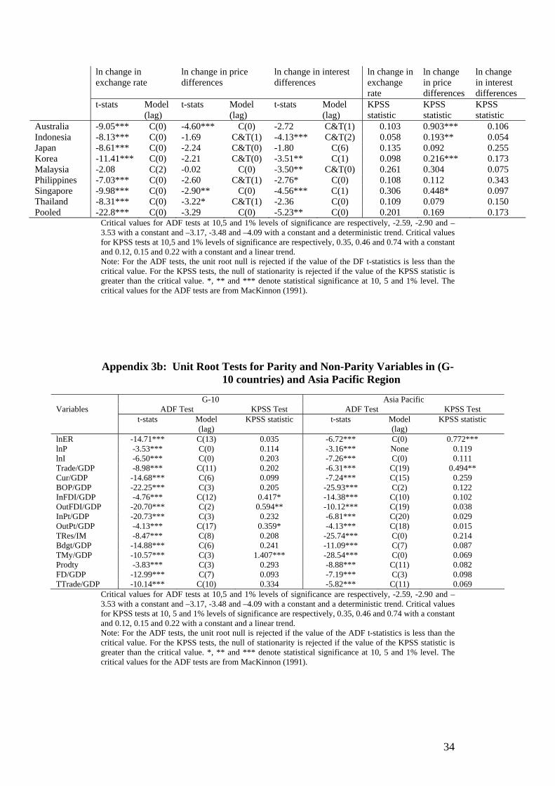
Appendix 3a: Unit Root Tests for Parity Variables in Asia Pacific

ADF Test KPSS Test

34

ln change in exchange rate

ln change in price differences

ln change in interest differences

ln change in exchange rate

ln change in price differences

ln change in interest differences

t-stats Model(lag)

t-stats Model (lag)

t-stats Model (lag)

KPSS statistic

KPSS statistic

KPSS statistic

Australia -9.05*** C(0) -4.60*** C(0) -2.72 C&T(1) 0.103 0.903*** 0.106 Indonesia -8.13*** C(0) -1.69 C&T(1) -4.13*** C&T(2) 0.058 0.193** 0.054 Japan -8.61*** C(0) -2.24 C&T(0) -1.80 C(6) 0.135 0.092 0.255 Korea -11.41*** C(0) -2.21 C&T(0) -3.51** C(1) 0.098 0.216*** 0.173 Malaysia -2.08 C(2) -0.02 C(0) -3.50** C&T(0) 0.261 0.304 0.075 Philippines -7.03*** C(0) -2.60 C&T(1) -2.76* C(0) 0.108 0.112 0.343 Singapore -9.98*** C(0) -2.90** C(0) -4.56*** C(1) 0.306 0.448* 0.097 Thailand -8.31*** C(0) -3.22* C&T(1) -2.36 C(0) 0.109 0.079 0.150 Pooled -22.8*** C(0) -3.29 C(0) -5.23** C(0) 0.201 0.169 0.173

Critical values for ADF tests at 10,5 and 1% levels of significance are respectively, -2.59, -2.90 and –3.53 with a constant and –3.17, -3.48 and –4.09 with a constant and a deterministic trend. Critical values for KPSS tests at 10,5 and 1% levels of significance are respectively, 0.35, 0.46 and 0.74 with a constant and 0.12, 0.15 and 0.22 with a constant and a linear trend. Note: For the ADF tests, the unit root null is rejected if the value of the DF t-statistics is less than the critical value. For the KPSS tests, the null of stationarity is rejected if the value of the KPSS statistic is greater than the critical value. *, ** and *** denote statistical significance at 10, 5 and 1% level. The critical values for the ADF tests are from MacKinnon (1991).

Appendix 3b: Unit Root Tests for Parity and Non-Parity Variables in (G-

10 countries) and Asia Pacific Region

G-10 Asia Pacific Variables ADF Test KPSS Test ADF Test KPSS Test t-stats Model

(lag) KPSS statistic t-stats Model

(lag) KPSS statistic

lnER -14.71*** C(13) 0.035 -6.72*** C(0) 0.772*** lnP -3.53*** C(0) 0.114 -3.16*** None 0.119 lnI -6.50*** C(0) 0.203 -7.26*** C(0) 0.111 Trade/GDP -8.98*** C(11) 0.202 -6.31*** C(19) 0.494** Cur/GDP -14.68*** C(6) 0.099 -7.24*** C(15) 0.259 BOP/GDP -22.25*** C(3) 0.205 -25.93*** C(2) 0.122 InFDI/GDP -4.76*** C(12) 0.417* -14.38*** C(10) 0.102 OutFDI/GDP -20.70*** C(2) 0.594** -10.12*** C(19) 0.038 InPt/GDP -20.73*** C(3) 0.232 -6.81*** C(20) 0.029 OutPt/GDP -4.13*** C(17) 0.359* -4.13*** C(18) 0.015 TRes/IM -8.47*** C(8) 0.208 -25.74*** C(0) 0.214 Bdgt/GDP -14.88*** C(6) 0.241 -11.09*** C(7) 0.087 TMy/GDP -10.57*** C(3) 1.407*** -28.54*** C(0) 0.069 Prodty -3.83*** C(3) 0.293 -8.88*** C(11) 0.082 FD/GDP -12.99*** C(7) 0.093 -7.19*** C(3) 0.098 TTrade/GDP -10.14*** C(10) 0.334 -5.82*** C(11) 0.069

Critical values for ADF tests at 10,5 and 1% levels of significance are respectively, -2.59, -2.90 and –3.53 with a constant and –3.17, -3.48 and –4.09 with a constant and a deterministic trend. Critical values for KPSS tests at 10, 5 and 1% levels of significance are respectively, 0.35, 0.46 and 0.74 with a constant and 0.12, 0.15 and 0.22 with a constant and a linear trend. Note: For the ADF tests, the unit root null is rejected if the value of the ADF t-statistics is less than the critical value. For the KPSS tests, the null of stationarity is rejected if the value of the KPSS statistic is greater than the critical value. *, ** and *** denote statistical significance at 10, 5 and 1% level. The critical values for the ADF tests are from MacKinnon (1991).