bond market intermediation and the role of repo · bond market intermediation and the role of repo...
TRANSCRIPT

Finance and Economics Discussion SeriesDivisions of Research & Statistics and Monetary Affairs
Federal Reserve Board, Washington, D.C.
Bond Market Intermediation and the Role of Repo
Yesol Huh and Sebastian Infante
2017-003
Please cite this paper as:Huh, Yesol, and Sebastian Infante (2017). “Bond Market Intermediation and the Role ofRepo,” Finance and Economics Discussion Series 2017-003. Washington: Board of Gover-nors of the Federal Reserve System, https://doi.org/10.17016/FEDS.2017.003.
NOTE: Staff working papers in the Finance and Economics Discussion Series (FEDS) are preliminarymaterials circulated to stimulate discussion and critical comment. The analysis and conclusions set forthare those of the authors and do not indicate concurrence by other members of the research staff or theBoard of Governors. References in publications to the Finance and Economics Discussion Series (other thanacknowledgement) should be cleared with the author(s) to protect the tentative character of these papers.

Bond Market Intermediation and the Role of Repo∗
Yesol Huh Sebastian Infante
Federal Reserve Board
December 12, 2016
Abstract
This paper models the important role that repurchase agreements (repos) play in bond
market intermediation. Not only do repos allow dealers to finance their activities, but they also
increase dealers’ ability to satisfy levered client demands without having to adjust their holdings
of risky assets. In effect, the ability to borrow specific assets for delivery allows dealers to source
large quantity of assets without taking ownership of them. Larger levered client orders imply
larger asset borrowing demands, thus increasing the borrowing cost for the asset (i.e., repo
specialness). Dealers pass on the higher intermediation cost to their clients in the form of
higher bid-ask spreads. Although this method of intermediation is optimal, the use of repos
significantly increases dealers’ balance sheets. Limiting one dealer’s balance sheet leverage,
leaving all else equal, reduces the affected dealer’s market making abilities and increases his
bid-ask spreads. The equilibrium effect of limiting all dealers’ balance sheet leverage on bid-
ask spreads is unclear, and depends on the intensity of clients’ demand and securities lenders’
sensitivity to repo specialness.
∗This paper was previously circulated under the title “Bond Market Liquidity and the Role of Repo.” We thank ErikHeitfield, Jean-David Sigaux, and participants at the 12th Annual Central Bank Conference on Market Microstructureof Financial Markets for their helpful feedback. The views of this paper are solely the responsibility of the authorsand should not be interpreted as reflecting the views of the Board of Governors of the Federal Reserve System orof any other person associated with the Federal Reserve System. Federal Reserve Board, 20th St. and ConstitutionAvenue, NW, Washington, DC, 20551. Please send comments to: [email protected].
1

1 Introduction
The perceived reduction in Treasury bond liquidity has become a highly debated topic among
market participants and policy makers. Many market participants have argued that regulations
such as the Supplementary Leverage Ratio (SLR) have made repurchase agreements (repos) more
expensive for dealers, and that this in turn has hurt liquidity in the cash Treasury market. While it
is well known that repos are widely used in cash market intermediation, especially for shorting, it is
not clear how limiting dealer leverage would translate to lower liquidity. Most market commentary
give matched book repos as an example of how leverage constraint would hurt the repo market.
However, given that funding is usually the driver of matched book repos, it is not clear whether it
should relate to cash market liquidity. In this paper, we aim to build a model that directly links
repo markets with cash market liquidity by modeling how dealers use repo to intermediate in the
cash market.
Repos give market makers the ability to finance and source assets without having to take
ownership of them. It has long been understood that dealers rely on repo as an important source
of funding, not only to finance their own positions, but also to finance counterparties’ activities. In
addition, repos, and more specifically, securities lending, play a critical role in enabling investors
to take short positions. In effect, a short sale requires a borrowed asset. This paper accounts
for these two roles that repo play, and also presents a third: to enable dealers to increase their
intermediation capacity without affecting their optimal portfolio choice. Figure 1 shows primary
dealers’ aggregate repo and trading volumes in the U.S. Treasury market. The high correlation
between these two series is suggestive of how important the repo market is for trading activity.
To show the above intuition, we present a two period model in which dealers service clients’
trading and financing needs by purchasing and borrowing a single risky asset. The model features
a continuum of dealers that intermediate for other investors, called clients, which seek to execute
trades. Each dealer is a monopolist to their clients, which submit levered long or short sale orders to
their dealer for execution. Client trade sizes are stochastic but depend on the bid/ask imposed by
the dealer: a larger markup lowers demand, reducing the probability of a larger order size. Dealers
trade in a centralized interdealer market to fill client orders, internalizing how trading affects their
2
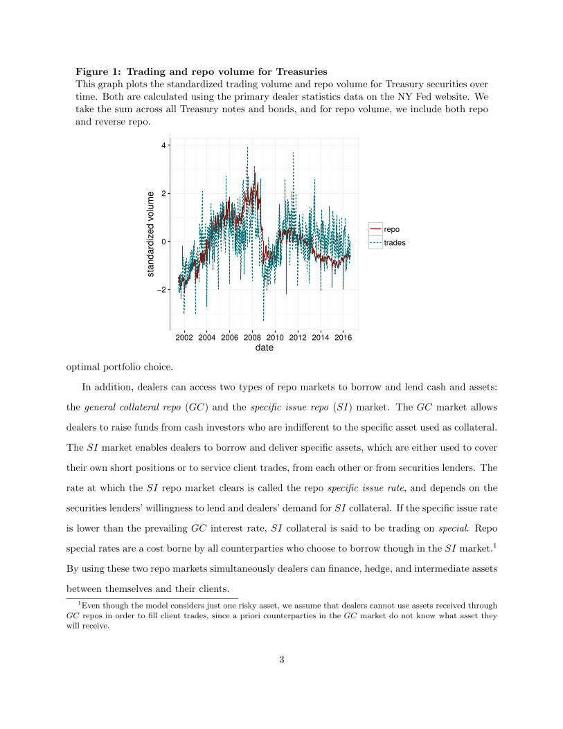
Figure 1: Trading and repo volume for TreasuriesThis graph plots the standardized trading volume and repo volume for Treasury securities overtime. Both are calculated using the primary dealer statistics data on the NY Fed website. Wetake the sum across all Treasury notes and bonds, and for repo volume, we include both repoand reverse repo.
−2
0
2
4
2002 2004 2006 2008 2010 2012 2014 2016
date
sta
ndard
ized v
olu
me
repo
trades
optimal portfolio choice.
In addition, dealers can access two types of repo markets to borrow and lend cash and assets:
the general collateral repo (GC) and the specific issue repo (SI) market. The GC market allows
dealers to raise funds from cash investors who are indifferent to the specific asset used as collateral.
The SI market enables dealers to borrow and deliver specific assets, which are either used to cover
their own short positions or to service client trades, from each other or from securities lenders. The
rate at which the SI repo market clears is called the repo specific issue rate, and depends on the
securities lenders’ willingness to lend and dealers’ demand for SI collateral. If the specific issue rate
is lower than the prevailing GC interest rate, SI collateral is said to be trading on special. Repo
special rates are a cost borne by all counterparties who choose to borrow though in the SI market.1
By using these two repo markets simultaneously dealers can finance, hedge, and intermediate assets
between themselves and their clients.
1Even though the model considers just one risky asset, we assume that dealers cannot use assets received throughGC repos in order to fill client trades, since a priori counterparties in the GC market do not know what asset theywill receive.
3
To satisfy client long or short demand, a dealer has to have the actual securities, either through
outright ownership or sourcing it via reverse repo. Dealers cannot write naked shorts or derivative-
like positions.2 This SI box constraint is a crucial friction in our model. In our model, clients do
fully levered long or short trades, that is, dealer will either sell the asset to the client and reverse
repo it in, or repo out the asset to the client and buy it back. Thus, the number of actual assets
that the dealer has in the box does not change after trading with the client. However, the SI box
constraint dictates that the dealer still has to have the asset in order to do this trade. Hence,
dealers may have to source in assets via the expensive SI repo market. The SI repo market
allows dealers to increase the amount of assets they can source—the amount of assets purchased
and borrowed—without compromising their risk adjusted return decision. That is, repos allow
dealers to maximize their market making ability, increasing market liquidity, while allowing them
to maintain an optimal risky asset position.
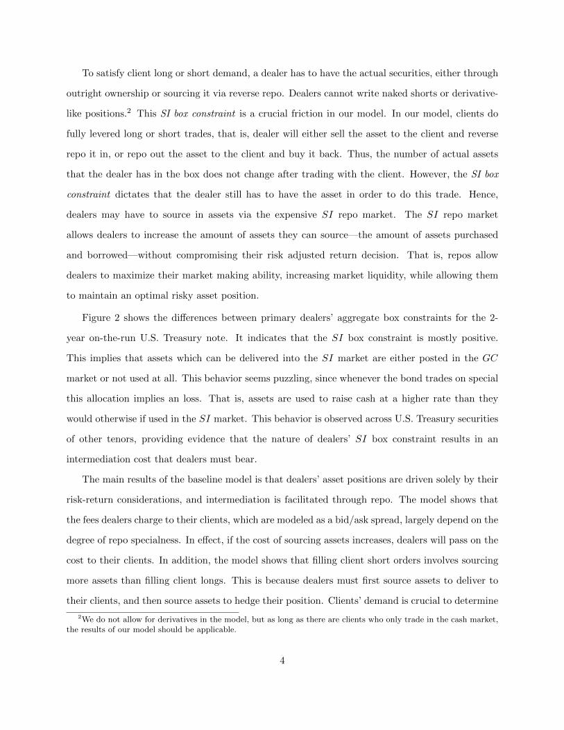
Figure 2 shows the differences between primary dealers’ aggregate box constraints for the 2-
year on-the-run U.S. Treasury note. It indicates that the SI box constraint is mostly positive.
This implies that assets which can be delivered into the SI market are either posted in the GC
market or not used at all. This behavior seems puzzling, since whenever the bond trades on special
this allocation implies an loss. That is, assets are used to raise cash at a higher rate than they
would otherwise if used in the SI market. This behavior is observed across U.S. Treasury securities
of other tenors, providing evidence that the nature of dealers’ SI box constraint results in an
intermediation cost that dealers must bear.
The main results of the baseline model is that dealers’ asset positions are driven solely by their
risk-return considerations, and intermediation is facilitated through repo. The model shows that
the fees dealers charge to their clients, which are modeled as a bid/ask spread, largely depend on the
degree of repo specialness. In effect, if the cost of sourcing assets increases, dealers will pass on the
cost to their clients. In addition, the model shows that filling client short orders involves sourcing
more assets than filling client longs. This is because dealers must first source assets to deliver to
their clients, and then source assets to hedge their position. Clients’ demand is crucial to determine
2We do not allow for derivatives in the model, but as long as there are clients who only trade in the cash market,the results of our model should be applicable.
4

0
4000
8000
12000
2013−07 2014−01 2014−07 2015−01 2015−07 2016−01 2016−07
date
Box (
in m
illio
n U
SD
)
A. 2yr Note
−5000
0
5000
10000
2013−07 2014−01 2014−07 2015−01 2015−07 2016−01 2016−07
date
Box (
in m
illio
n U
SD
)
B. 10yr Note
Global box SI box
Figure 2: SI box and global box for primary dealers.SI box and global box is calculated from FR 2004 data downloaded from NY Fed website. SIbox is defined as net position plus the reverse repo on specific issue minus the repo on specificissue. Global box is defined as SI box plus reverse repo on general collateral minus the repo ongeneral collateral. Panel A. calculates the SI box and global box for the 2 year Treasury note,and Panel B. calculates for the 10 year Treasury note.
5

the degree of asset specialness, the cost of intermediation, and ultimately market liquidity. We also
show that an increase in securities lenders’ willingness to lend decreases specialness and bid-ask
spreads.
Although this method of intermediation is optimal, it has its drawbacks. Specifically, it involves
engaging in various repos and reverse repos, which can substantially increase the size of a dealer’s
balance sheet. Motivated by the recent regulatory initiatives to limit the amount of leverage a large
bank holding company (BHC) can take, we impose an additional restriction that limits dealers’
balance sheet size. We show that this size limit reduces dealers’ incentives to intermediate large
trades, and dealers cap the amount of client orders they fill, thus limiting market depth. In the
partial equilibrium setting, dealers increase the bid-ask spread, although in the general equilibrium
setting the result is ambiguous since a cap on repo intermediation also puts downward pressure
on repo specialness, alleviating the direct cost of intermediation. Additionally, if the size limit
becomes tighter for a given dealer, it will increase the bid-ask spread that it quotes.
We do not attempt to make a statement about whether leverage restrictions are welfare im-
proving or deteriorating in this paper. Because we assume contract enforceability and no limited
liability, there are no negative consequences associated with large dealer balance sheets. Discussing
the benefits of leverage constraints is outside the scope of this paper; thus, the results that leverage
constraints decrease intermediation and potentionally market liquidity should be interpreted with
the above caveat in mind. We also do not include other possible sources of liquidity, such as high
frequency traders. However, to the extent that the intermediation in dealer-customer market in
Treasury securities are dominated by dealers, this omission is not a serious issue.
The paper is structured as follows. Section 2 reviews related literature, and Section 3 gives
some institutional background on the different repo markets in the United States and the role
dealers play. The following section describes the model setup, detailing the main agents and how
they interact. Section 5 presents the symmetric equilibrium and interpretation when dealer balance
sheets are unrestricted. Section 6 incorporates restrictions on the size of dealers’ balance sheet and
shows how this affects their markup decision.
6

2 Literature Review
Our paper is related to the literature on Treasury market liquidity. Using high frequency data
from the interdealer market, Fleming and Remolona (1999) studies how price and bid-ask spreads
change around macroeconomic announcements. Fleming (2003) compares different liquidity mea-
sures, and finds that bid-ask spread and price impact measures are more informative than other
liquidity measures such as quote size and on-the-run/off-the-run yield spreads. Mizrach and Neely
(2006) studies how liquidity changed when the Treasury interdealer market transitioned from voice
to electronic markets, and Fleming (1997) documents the intraday patterns of Treasury market
liquidity. Goldreich et al. (2005) relates the on-the-run/off-the-run price difference to the auction
cycle. These papers study the cash market without considering repo markets and focus on the
interdealer markets, as there is very little data on the over-the-counter dealer-customer markets.
More directly related to our paper are the studies on repos and their specialness, and the asset
pricing implications. First documented by Duffie (1996), repo specialness refers to a significantly
low repo rate paid to borrow a security that is in high demand. Duffie (1996) shows that the
degree of repo specialness depends on the demand for short positions and the supply of loanable
collateral, and provides a theoretical relationship between bond prices and repo specialness. Jordan
and Jordan (1997) document this pricing relationship empirically. Krishnamurthy (2002) studies
the spread between newly issued U.S. Treasuries (termed on-the-run) and existing securities of
similar characteristics (termed off-the-run). He shows that trading profits from shorting on-the-
run securities and buying existing securities are close to zero due to different repo financing costs:
on-the-run securities can trade on special implying a significant shorting cost. D’Amico et al.
(2015) studies the supply and demand factors that drive repo specialness, focusing on the Federal
Reserve’s purchase programs.
The on-the-run/off-the-run price or yield differences that are studied in these papers are often
used as a measure of liquidity in Treasury markets, as the price difference may be due to the liquidity
premium embedded in the more-liquid on-the-run security. To that extent, these papers can be
thought of as studying how repo markets affect cash market liquidity and vice versa. However, as
Krishnamurthy (2002) points out, the price difference may simply due to cost of arbitrage stemming
7

from repo specialness. Our main object of interest is the bid-ask spread, which is a more direct
measure of liquidity. We also allow price to change due to change in repo specialness, similar to
Krishnamurthy (2002); however, we only have one asset, so there is no arbitrage relationship, and
we do not model liquidity premium.
In terms of the model setup, our model is closest to the literature on how market makers’
inventory management affects their liquidity provision. In a setting where dealers are risk averse
or have constraints on the size of their inventory, dealers adjust their quotes to change order flow
so that they can bring the inventory size back to their optimal position. Amihud and Mendelson
(1986) model a monopolistic, risk-neutral dealer with inventory size constraints. Stoll (1978) model
a risk-averse monopolistic dealer, while Ho and Stoll (1983) model a market with multiple dealers.
In most of these models, while the prices that dealers quote will change the order arrival rate of
buy and sell trades, it is still probabilistic, and they have to wait until it arrives. In some models,
dealers may trade in the interdealer market to offset the inventory, as in Ho and Stoll (1983). Since
there is a finite number of dealers in that model, they behave strategically and may sometimes opt
to bear inventory risk instead of laying it off in the interdealer market.
Our model has some similarities and differences with other models in this literature. As in the
above papers, dealers are risk-averse and have to be compensated for deviating from their optimal
portfolio. Also, the bid and ask spreads set by the dealers affect customer demand, but in our
setup, dealer quotes alter the order size rather than the order arrival rate. Because our focus
is on the intersection of repo markets and market making, we simplify other dimensions relative
to the existing literature. We have a continuous mass of dealers and a frictionless interdealer
market, thus dealers can easily lay off inventory risk through the interdealer market. Frictionless
interdealer markets, and the ability to source assets through repo, allows dealers to intermediate
trades without compromising their optimal portfolio. For simplicity we assume each dealer has a
separate set of customers, therefore they do not compete to attract customer order flows. Another
crucial difference is that in our model, dealers first need to source the securities in order to facilitate
trade.
The paper is also related to the large literature on trading frictions in securities markets. In
8

particular, Bottazzi et al. (2012) show how asset and repo markets coexist in a stylized general
equilibrium framework. In that paper the authors underscore a particularly relevant restriction
that securities dealers must satisfy: the box constraint. This constraint forces intermediaries to
borrow a security whenever they want to short. Our paper focuses on a particular market structure,
where clients pay dealers to service trades, which allows us to gauge the degree of market liquidity
through dealer markups. We also consider two distinct repo markets for the same underlying
collateral, SI and GC repo markets, which are used either to source or to finance assets and are
subject to different box constraints.
Lastly, securities lenders are also play an important role in the repo market. Foley-Fisher et al.
(2015) argue that securities lenders are not merely responding to the demand to borrow securities,
but they also use securities lending as a way to finance long-term asset positions. To this end,
we model the supply of assets from securities lenders as not only responding to changes in repo
specialness, but also as having a free parameter which reflects their willingness to supply assets.
We look at how the equilibrium changes with their willingness parameter.
3 Institutional Setting
In the United States, there are two distinct repo markets. The most commonly known is the U.S.
tri-party repo market. This market is considered a wholesale funding market, where financial firms,
typically large broker-dealers, can raise short term secured debt from cash investors. In this repo
market, given a certain collateral class, borrowers have the flexibility to choose from a range of
assets that they may post as collateral. In effect, cash lenders in this market only value collateral
as a back-stop to a borrower default, implying a wide variety of collateral is acceptable. This
makes the tri-party market a GC repo market. The tri-party market’s collateral flexibility is also
valued by cash borrowers, who can manage their collateral holdings by exchanging assets within
a collateral class whenever different asset demands arise. In this market, a clearing agent stands
between cash borrowers and lenders, providing clearing services and extending intraday credit to
9

borrowers who may need to access their asset during the day.3
The second repo market is known as the bilateral repo market, where trades are made bilaterally
and can be tailored to accommodate specific needs. Importantly, trades in the bilateral market
can be against specific collateral, allowing investors to borrow a particular asset in order to short
sell or deliver to another counterparty. This makes the bilateral market an SI repo market. When
demand for borrowing a specific issue is high, the bilateral repo rate can be lower than the tri-
party repo rate. This incentivizes the original collateral owners to lend their securities to reap the
difference between GC and SI repo rates. It is important to note that bilateral repos are also an
important means of funding for investors who do not qualify to participate in the tri-party market.
These lower quality firms typically issue bilateral repos to large dealers, who in turn access the
tri-party market to raise funds for the initial repo; a process known as rehypothecation.
Dealers are the primary market participants who access both repo markets. They use the tri-
party market to raise funds and manage collateral, and use the bilateral market to source assets and
fill client demands. Dealer counterparties in the bilateral market are their client base who demand
trading and financing services, and securities lenders who effectively lend their securities to receive
cash at the special rate. Cash investors in the tri-party market are largely money market funds
and securities lenders who reinvest the cash received in their securities lending activities. Adrian
et al. (2013) have a more detailed overview on how these markets are related and the role securities
dealers play.
4 Model Setup
The model consists of 3 periods t ∈ {0, 1, 2}. In t = 0, dealers post their bid and ask to clients.
At t = 1, client orders are realized, and order sizes are smaller for larger bid/ask spreads. Dealers
receive both buy and sell orders, a fraction of which will be levered. That is, a portion of client
orders will be a cash and repo trade with the dealer simultaneously, establishing either levered long
or short positions. Throughout the model, we will assume SI repos will be trading special, which
3In recent years the tri-party market has been reformed to reduce the amount of intraday credit needed for dealersto access their assets. More information on tri-party reform can be found in http://www.newyorkfed.org/banking/
tpr_infr_reform.html.
10

t = 0
Dealers post bid/ask
t = 1
Client orders arriveDealers fill ordersInterdealer trade
t = 2
Asset uncertainty realizedCash flows distributed
Figure 3: Model Timeline
implies that dealers have to bear a cost to source a specific asset.
4.1 Assets & Contracts
The risky asset will have a final payoff given by v ∼ N(µ, σ). We assume that there is an unrestricted
secured lending market for GC repos with an exogenously specified one-period risk-free rate R. This
means there is an abundance of cash and GC assets from outside investors. Only secured debt is
allowed (i.e., repo) to raise funding.
The price of the risky asset p and the specific issue repo rate RS will be determined by market
clearing. We will consider settings where in equilibrium, the repo rate on SI repos are below the
risk free rate: RS < R. The main difference between SI and GC repos is that dealers can use SI
repos to establish short positions and deliver them to their clients.
For simplicity, we assume that repos do not have haircuts, yet are risk free, which happens
since we assume contract enforceability and no limited liability. This assumption simplifies the
analysis greatly and keeps the focus on dealers’ use of repo to borrow assets in order to deliver
them to clients. We can relax this assumption somewhat by incorporating haircuts to make GC
repos “virtually risk free”4 and by allowing dealers to charge different haircuts to their clients,
depending on whether they submit a levered long or short sale.5 Adding these features complicates
the analysis without significantly altering the results.6
The model’s state variables in t = 0 are dealers’ initial asset position D and dealers’ initial cash
holdings W . Although these initial variables are not crucial to the theoretical model, they allow us
to better interpret the data. In terms of notation, a repo using Q assets as collateral implies that
4The case of virtually risk free can be interpreted as repos with U.S. Treasuries that have a 2% haircut.5Infante (2015) shows that SI repo haircuts can be negative whenever investors need to source an asset.6The assumption on repos’ riskiness implies that the current version of the model is not well suited to study
systemic risks that come from rehypothecation.
11

the cash borrower receives pQ in funds and distributes Q in risky assets to the cash lender. On the
closing leg of the repo, the cash lender of a repo receives R × pQ or RS × pQ in cash, depending
on whether it was a GC or SI repo, and returns the asset back to the cash borrower. It is useful
to denote repo contracts by the amount of assets delivered as collateral rather than total amount
borrowed or lent since it underscores the impact of box constraint.
4.2 Agents
There are three types of agents in the economy: dealers, securities lenders, and clients. Each client
con only interact with one dealer; thus, there is no outright competition between dealers. Dealers
are endowed with an initial portfolio in t = 0, but will have the ability to rebalance their position
once a client order is received. Dealers service their client orders, which may be be buys or sales,
or levered long or short positions. Securities lenders are long-term investors who already hold their
optimal portfolio in t = 0, but have the ability to lend their securities to dealers.
4.2.1 Dealers
There is a continuum of dealers with CARA utility and risk aversion γ which consume the payoff
from their portfolio in the final period. Specifically, their final payoff consists of cash flows from their
risky investments, payoff from their repos, and fees in the form of bid/ask from clients. Therefore,
a dealer’s final wealth takes the following form:
W2 = (v − p)QD + (RS − 1)pQSR + (R− 1)pQGR
−(v − φLRSp)QL + (v − φSRSp)QS + (1− φL)pQL − (1− φS)pQS + apQL + bpQS
+vD +W
where QD is the dealer’s portfolio rebalancing in the cash market, QSR is the amount of assets
sourced through SI repos, and QGR the amount of assets received as collateral through GC repos
(i.e. cash lending); all are chosen in t = 1.7 Transactions with clients are not included in QD, QSR,
7Since our model is a one-shot trading game, there are no rollover risks. If there are multiple periods where repotrading happens, dealers face the risk that the cash borrower may not want to roll over the overnight repo, or roll
12

and QGR. The second line in expression (1) highlights the effect of clients’ orders on the dealer’s
portfolio. The size of a client’s buy and sale orders are given by QL and QS , of which a fraction
φL and φS are accompanied by repo orders, respectively. Note that a client buy order implies a
negative position for the dealer, thus it is associated with a −(v − p). D is the dealer’s initial
portfolio position and W is the amount of cash the dealer has initially. D and W characterize the
dealer’s initial portfolio endowment, and we assume W + pD > 0. Finally, apQL and bpQS are the
profits from the bid (b) and ask (a) spreads. The dealer chooses a and b at t = 0, and the tradeoff is
between spreads and intermediation quantity. Note that in this setup, dealers charge their clients
in the form of bid/ask spreads, but the model is equivalent to a case where dealers use other forms
of contracting arrangements to charge their clients, such as repo markups.
The main restrictions for dealers are their global and SI box constraint. The total amount
of assets (SI and GC) must always be non-negative, and the amount of SI assets the dealer can
access must be large enough to cover the clients’ levered orders. Specifically, we assume dealers’
SI box restriction is a function of levered orders: g(φQL, φQS) > 0. This assumption captures the
intuition that dealers need to, at least in part, access assets in order to establish client positions.8
Specifically, given client order sizes QL = QL and QS = QS , the dealer’s SI box constraint is given
by,
D +QD +QSR − (1− φL)QL + (1− φS)QS ≥ g(φQL, φSQS). (1)
That is, the total amount of SI assets the dealer can access—its initial holdings, its assets bought
in the interdealer market, assets source via SI repos, and unlevered buy/sell orders which alters
the dealer’s inventory—must be enough to deliver to its levered clients in the form of g. Note
that with levered long and short orders, the dealer will get back the asset it buys (sells) and lends
to (borrows from) their client, but we assume that the dealer must have g assets to facilitate
these levered trades. Without such an assumption, the dealer would be able to do infinitely many
levered trades with its clients.9 Although the presence of g implies a cost that dealers must bear to
over at unfavorable rates. This potentially may have a large effect.8In effect, if g = 0, dealers would be able to write “naked” shorts and longs with their clients.9This assumption incorporates a friction that will decouple the cash market from the SI repo market, similar to
13
intermediate levered trades, there is suggestive evidence that the friction exists. In effect, Figure
2 shows the right hand side of U.S primary dealers SI and GC box constraint for 2 and 10 year
on-the-run Treasury note. The difference between the two lines is the empirical counterpart of g,
which is almost always positive.10 Table 1 shows summary statistics on the size of the SI and GC
box constraint, and the fraction of the time where the former is greater than zero.
4.2.2 Securities Lenders
We model securities lenders in a reduce form to focus on dealer behavior. Securities lenders lend
assets through SI repos based on a reduced form supply function SL(R−RS ; η) with ∂SL∂(R−RS) > 0.
That is, the more the repo trades on special, the more securities lenders are willing to lend. We
also assume that the supply from securities lenders depends on η, which governs their willingness to
provide securities lending services. In effect, Foley-Fisher et al. (2015) show that securities lending
programs use funds from their activities to finance long dated assets, making their lending services
depend on factors beyond repo specialness. We capture these incentives in reduced form through
η, and assume ∂SL∂η > 0.
4.2.3 Clients
Client order sizes are stochastic and exogenously specified. Specifically, the size of client orders are
independent and distributed QL, QS ∼ Exp(λ(x)) (x ∈ {a, b}), where λ is a function of the dealer’s
bid/ask quote. We assume λ, λ′, and λ′′ ≥ c > 0 where c is an arbitrarily small constant. Clients
can be interpreted as liquidity traders, who can only access one dealer, and are price sensitive to
the dealer’s markup: their trade sizes depend on their dealer’s bid/ask quote.
Note that a levered client order is in fact two transactions: an asset purchase (sale) with a client
repo (reverse repo).
Krishnamurthy (2002).10Specifically, the difference shows the amount of on-the-run assets which are posted as collateral in the GC market,
which as we will show, constitutes an intermediation cost dealers must bear.
14
4.3 Market Structure Summary
To summarize our setup, Figure 4 illustrates how dealers distribute collateral between all three
markets: cash, SI repo, and GC repo; and the role securities lenders and clients play. Clients will
approach a dealer and submit buy (QL) and sell (QS) orders, a fraction φL and φS of which will
be accompanied by repos and reverse repos, respectively. After clients order flow is realized, the
dealer will access three markets. The cash market will serve to buy and sell securities for dealers to
rebalance their risky asset position. The GC repo market will allow dealers to raise or invest funds
at the GC repo rate. The SI repo market will allow dealers to either source assets to satisfy their
SI box constraint or deliver assets to raise relatively cheap funding. Finally, securities lenders will
provide assets to the SI repo market as a function of repo specialness and their willingness to lend
assets.
5 Optimal Strategies and Symmetric Equilibrium in Unrestricted
Case
In this section, we solve for dealers’ optimal strategies in t = 1. Here we shall assume that
dealers have no balance sheet restrictions. For simplicity, we characterize the resulting symmetric
equilibrium. We then turn to the optimal bid/ask which determines the order intensity.
5.1 Optimal Strategies & Equilibrium in Interdealer Market
Given an initial total position D,W and order size QL = QL and QS = QS , the dealer’s final payoff
takes the expression in equation (1). Therefore, the dealer solves the following problem,
max{QD,QSR,Q
GR}
E(u(W2)|QL = QL, QS = QS),
15

Figure 4: Model Market StructureD stands for dealer, C stands for a dealer’s client, Sec Lender stands for the securities lender.The dealer receives client long and sale ordersQL andQS , a fraction φL and φS are accompaniedby repos and reverse repos, respectively. GC Market stands for general collateral market, SIMarket stands for specific issue collateral market, and Cash Market stands for the underlyingasset market. Upon receiving client orders, a dealer chooses how much collateral to sourceor deliver to the GC market (QGR) and the SI market (QSR), and how much to buy or sell inthe cash market (QD). Positive QGR or QSR means that the dealer is engaging in reverse repos.Positive QD means that the dealer is buying the asset. Securities lenders supply SL assets tothe SI market. Only the asset movements (either through outright purchases and sales or asrepo collateral) are drawn. Straight arrows indicate outright sales, and curved arrows indicaterepo collateral movements.
D
Cash Market
GC Market
SI
Mar
ket
CQL −QS
φLQS
φSQSQD
QSR
QGR
Sec.Lender
SL
16
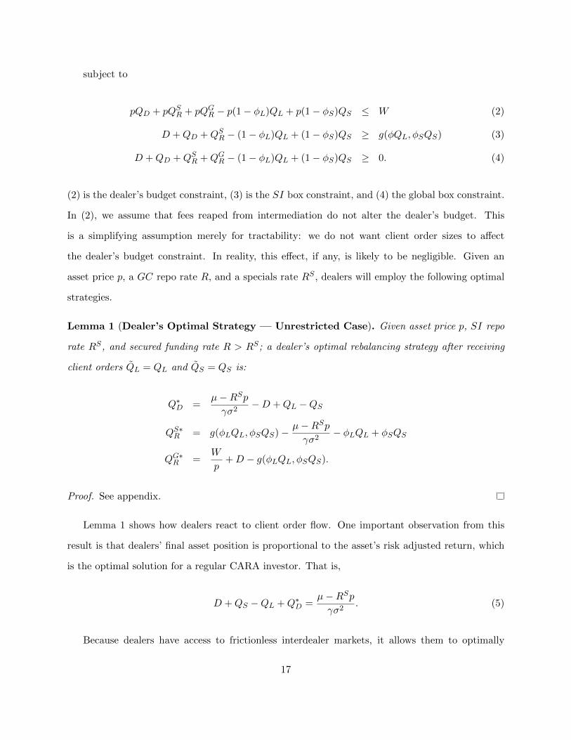
subject to
pQD + pQSR + pQGR − p(1− φL)QL + p(1− φS)QS ≤ W (2)
D +QD +QSR − (1− φL)QL + (1− φS)QS ≥ g(φQL, φSQS) (3)
D +QD +QSR +QGR − (1− φL)QL + (1− φS)QS ≥ 0. (4)
(2) is the dealer’s budget constraint, (3) is the SI box constraint, and (4) the global box constraint.
In (2), we assume that fees reaped from intermediation do not alter the dealer’s budget. This
is a simplifying assumption merely for tractability: we do not want client order sizes to affect
the dealer’s budget constraint. In reality, this effect, if any, is likely to be negligible. Given an
asset price p, a GC repo rate R, and a specials rate RS , dealers will employ the following optimal
strategies.
Lemma 1 (Dealer’s Optimal Strategy — Unrestricted Case). Given asset price p, SI repo
rate RS, and secured funding rate R > RS; a dealer’s optimal rebalancing strategy after receiving
client orders QL = QL and QS = QS is:
Q∗D =µ−RSpγσ2
−D +QL −QS
QS∗R = g(φLQL, φSQS)− µ−RSpγσ2
− φLQL + φSQS
QG∗R =W
p+D − g(φLQL, φSQS).
Proof. See appendix.
Lemma 1 shows how dealers react to client order flow. One important observation from this
result is that dealers’ final asset position is proportional to the asset’s risk adjusted return, which
is the optimal solution for a regular CARA investor. That is,
D +QS −QL +Q∗D =µ−RSpγσ2
. (5)
Because dealers have access to frictionless interdealer markets, it allows them to optimally
17
adjust their portfolio to accommodate their clients’ trades. Figure 5 shows how dealers rebalance
portfolio. To better show the intuition, we consider a simple example where the dealer only receives
a buy or sale order. That is, either (QL, QS) = (Q, 0) or (QL, QS) = (0, Q). Additionally, assume
φL = φS = 1
D =µ−RSpγσ2
g(QL, QS) = Q.
Then, if the dealer receives a client short order, its optimal strategy will be
Q∗D = −Q
QS∗R = 2Q−D
QG∗R =W
p+D −Q.
This is shown in Panel (a) of Figure 5. To maintain its optimal portfolio, the dealer wants to sell
Q of the risky assets in the interdealer market. However, to do so, it has to source an additional Q
assets from the SI repo market because of g; thus, it will source 2Q −D assets. Note that in the
client long scenario, this does not happen as the dealer buys Q from the interdealer market.
Aggregating all interdealer cash market trades gives the following market clearing condition for
the cash market. Here we denote each dealer’s demand with a subscript i to highlight that the
equilibrium price is determined by aggregating across all dealers.
∫iQDidi = 0. (6)
The SI repo market, which also incorporates securities lenders’ asset supply, clears through the
following equation, ∫iQSRidi = SL(R−RS ; η). (7)
Denoting by∫iDdi dealers’ aggregate position at the beginning of period t = 0, and assuming
18

Figure 5: Simple example
These diagrams show the dealer’s optimal solution in a simple case where W = 0, D = mu−RSpγσ2 ,
φL = φS = 1, and clients either submit a levered long order (panel (a)) or a short order (panel(b)). D stands for dealer, C stands for a dealer’s client, Sec Lender stands for the securitieslender. GC Market stands for general collateral market, SI Market stands for specific issuecollateral market, and Cash Market stands for the underlying asset market. Dealers optimallychoose how much collateral to source or deliver in the GC market, the SI market, and howmuch to buy or sell in the cash market. Only the asset movements (either through outrightpurchases and sales or as repo collateral) are drawn. Straight arrows indicate outright sales,and curved arrows indicate repo collateral movements. g stands for g(QL) in panel (a) andg(QS) in panel (b).
(a) Client Long
D C
Cash Market
GC Market
SI
Mar
ket
QL
QL
QL
QL +D − gg −D
(b) Client Short
D C
Cash Market
GC Market
SI
Mark
et
QS
QSQS
g +QS −D
g −D
19

symmetric strategies gives∫iDdi = D.
Proposition 1 (Interdealer Equilibrium — Unrestricted Case). Given dealers’ initial posi-
tion W and D, with W + pD > 0, GC repo rate of R, securities lending function sufficiently small
enough, and symmetric dealer bid and ask spreads a and b, dealers’ optimal strategies characterized
in Lemma 1 result in an asset price p and SI repo rate RS < R which solves the following system
of equations:
µ−RSpγσ2
= D − P(CL)
λ(a)+
P(CS)
λ(b)(8)
SL(R−RS ; η) = E(g(φLQL, φSQS))−D +(1− φL)P(CL)
λ(a)− (1− φS)P(CS)
λ(b)(9)
where P(CL) and P(CS) are the probability of a client long and short order, respectively.
Proof. The proof stems from considering dealers’ strategies in Lemma 1, imposing market clearing
conditions (6) and (7), and applying the law of large numbers for client orders.
Equation (8) shows how the price responds to client order flow: An increase in client longs
increases the price, whereas an increase in client shorts reduces the price. Equation (9) highlights
what drives repo specialness. Specifically, if there are larger frictions, namely if dealers need to hold
more assets to service levered longs and shorts, captured through a higher g, then dealers need to
source more assets in the SI market which puts upward pressure on repo specialness. In addition,
changes in φL orφS changes the amount of assets in the market due to unlevered client order flow;
giving a predictable effect on repo specialness.
It is interesting to note that considering the SI market clearing condition in isolation gives
SL(R−RS ; η) = E(g(φLQL, φSQS))−(µ−RSpγσ2
)− φLP(CL)
λ(a)+φSP(CS)
λ(b).
The above partial equilibrium equation highlights what market participants often comment regards
repo specialness: an increase in client short base increases repo specialness. In effect, if φS increases,
R−RS would need to increase to clear the market. But this observation neglects the effect of repo
specialness on the asset price. The general equilibrium solution in (9) shows that what matters
20
is the total amount of assets added and subtracted from the interdealer market, along with any
frictions associated with intermediating levered trades.
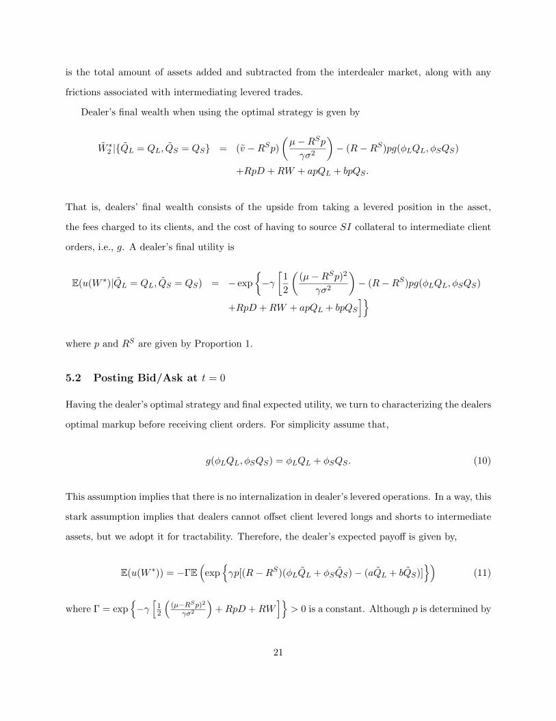
Dealer’s final wealth when using the optimal strategy is gven by
W ∗2 |{QL = QL, QS = QS} = (v −RSp)(µ−RSpγσ2
)− (R−RS)pg(φLQL, φSQS)
+RpD +RW + apQL + bpQS .
That is, dealers’ final wealth consists of the upside from taking a levered position in the asset,
the fees charged to its clients, and the cost of having to source SI collateral to intermediate client
orders, i.e., g. A dealer’s final utility is
E(u(W ∗)|QL = QL, QS = QS) = − exp
{−γ[
1
2
((µ−RSp)2
γσ2
)− (R−RS)pg(φLQL, φSQS)
+RpD +RW + apQL + bpQS
]}
where p and RS are given by Proportion 1.
5.2 Posting Bid/Ask at t = 0
Having the dealer’s optimal strategy and final expected utility, we turn to characterizing the dealers
optimal markup before receiving client orders. For simplicity assume that,
g(φLQL, φSQS) = φLQL + φSQS . (10)
This assumption implies that there is no internalization in dealer’s levered operations. In a way, this
stark assumption implies that dealers cannot offset client levered longs and shorts to intermediate
assets, but we adopt it for tractability. Therefore, the dealer’s expected payoff is given by,
E(u(W ∗)) = −ΓE(
exp{γp[(R−RS)(φLQL + φSQS)− (aQL + bQS)]
})(11)
where Γ = exp{−γ[12
((µ−RSp)2
γσ2
)+RpD +RW
]}> 0 is a constant. Although p is determined by
21

market clearing in t = 1, p is already known in t = 0. This is because dealer know all other dealers’
strategies, and also know the actual client order distribution due to the law of large numbers.
Integrating over QL and QS gives,
E(u(W ∗)) = −Γλ(a)
(λ(a) + γpa− γp(R−RS)φL)
λ(b)
λ(b) + γpb− γp(R−RS)φS)(12)
For the integral to exist, we need λ(a)+γpa−γp(R−RS)φL > 0 and λ(b)+γpb−γp(R−RS)φS > 0.
Recall that dealers do not internalize the effect of their optimal strategy on the price or specials
rate. This leads to the following Lemma on dealers’ optimal bid/ask.
Lemma 2 (Dealer’s Optimal Bid/Ask — Unrestricted Case). Given a dealer’s initial posi-
tion W and D, with W + pD > 0, GC repo rate of R, securities lending function sufficiently small
enough, and g as in (10); the dealer’s optimal bid and ask spread solve the following equations
λ′(a∗)a∗ − λ(a∗)− λ′(a∗)(R−RS)φL = 0
λ′(b∗)b∗ − λ(b∗)− λ′(b∗)(R−RS)φS = 0,
with a∗ > (R−RS)φL and b∗ > (R−RS)φS.
Proof. Taking the first order condition of expression (12), deduced from Proposition 1 with g as in
equation (10) gives the Lemma’s optimality conditions. In addition, note that a∗ > (R − RS)φL
and b∗ > (R−RS)φS because
∂E(u(W ∗))
∂a
∣∣∣a=(R−RS)φL
= −Γλ(b)
λ(b) + γpb− γp(R−RS)φS×
−λ((R−RS)φL)γp
(λ(a) + γpa− γp(R−RS)φL)2> 0,
implying a∗ > (R−RS)φL. The same argument holds for b∗.
Note that each individual dealer’s bid and ask spread is increasing in repo specialness. Because
dealers need to source g assets in order to intermediate, forcing them to bear the cost of repo
specialness, they pass on those costs to their clients. That is, from a partial equilibrium setting,
22
client’s market liquidity is decreasing in repo specialness.
Note that the optimal bid and ask in Lemma 2 do not depend on the underlying asset’s price.
This feature will be useful when characterizing how liquidity changes with securities lending activity.
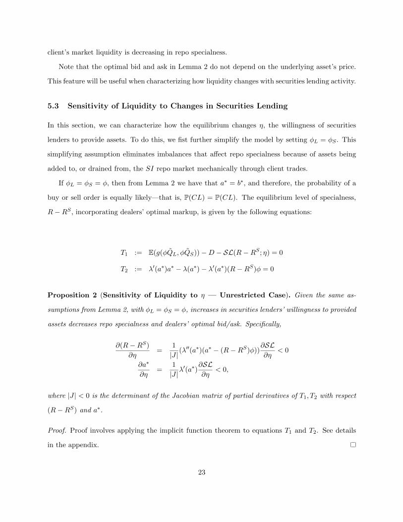
5.3 Sensitivity of Liquidity to Changes in Securities Lending
In this section, we can characterize how the equilibrium changes η, the willingness of securities
lenders to provide assets. To do this, we fist further simplify the model by setting φL = φS . This
simplifying assumption eliminates imbalances that affect repo specialness because of assets being
added to, or drained from, the SI repo market mechanically through client trades.
If φL = φS = φ, then from Lemma 2 we have that a∗ = b∗, and therefore, the probability of a
buy or sell order is equally likely—that is, P(CL) = P(CL). The equilibrium level of specialness,
R−RS , incorporating dealers’ optimal markup, is given by the following equations:
T1 := E(g(φQL, φQS))−D − SL(R−RS ; η) = 0
T2 := λ′(a∗)a∗ − λ(a∗)− λ′(a∗)(R−RS)φ = 0
Proposition 2 (Sensitivity of Liquidity to η — Unrestricted Case). Given the same as-
sumptions from Lemma 2, with φL = φS = φ, increases in securities lenders’ willingness to provided
assets decreases repo specialness and dealers’ optimal bid/ask. Specifically,
∂(R−RS)
∂η=
1
|J |(λ′′(a∗)(a∗ − (R−RS)φ))
∂SL∂η
< 0
∂a∗
∂η=
1
|J |λ′(a∗)
∂SL∂η
< 0,
where |J | < 0 is the determinant of the Jacobian matrix of partial derivatives of T1, T2 with respect
(R−RS) and a∗.
Proof. Proof involves applying the implicit function theorem to equations T1 and T2. See details
in the appendix.
23

Proposition 2 shows that as securities lenders provide more assets into the market through repos,
the amount of repo specialness and dealers’ markup decrease. Both of these changes are intuitive.
More assets to borrow reduces the degree of repo specialness. And because repo specialness is a
cost borne by dealers, they pass those savings onto their clients. This result highlights the tight link
between repo specialness and market liquidity. This also implies that not only would reverse repo
operations by the Federal Reserve decrease repo specialness (D’Amico et al. (2015)), but would
also increase liquidity in the cash Treasury market.
6 Optimal Strategies and Symmetric Equilibrium in Restricted
Balance Sheet Case
The analysis in Section 5 assumed that dealers had the liberty to alter the size of their balance
sheets to accommodate arbitrarily large client orders. But since the financial crisis, broker-dealers
affiliated with Bank Holding Companies (BHCs) are subject to a number of regulatory restrictions in
an effort to make these BHCs more resilient. One of these regulatory initiatives, the Supplementary
Leverage Ratio (SLR), restricts the amount of leverage a large BHC can take.
In the context of our model, the specific functional form of the leverage ratio restriction used
in the SLR would be difficult to model. But, assuming the the BHC has a fixed level of equity, a
leverage restriction can be translated into a size restriction on the dealer’s balance sheet. In order
to understand how this restriction may affect the dealer’s intermediation activities, we first have
to translate the model’s outcome onto a balance sheet.
Given the additional complexity of incorporating a limit on dealers’ balance sheet, this section
will adopt a number of simplifying assumptions relative to the general model presented in Section
4. First, we assume that each dealer receives only one levered long or short order.11 These orders
can still be arbitrarily large, but the focus is on how each of them affect the dealer’s ability to
intermediate. Given that each dealer will receive one client order, g will be a function of that
order’s size.
11This implies that φL = φS = 1.
24
Without loss of generality, we will assume that µ > RSp, which implies that dealers’ unrestricted
optimal asset position is positive. To simplify dealers’ initial size, we assume all dealers’ initial asset
position is D = 0, and their initial wealth W > 0 is arbitrarily small.
The innovation of this section is that dealers have an upper bound C on the size of their balance
sheet. Given that the dealer’s balance sheet composition is different for long and short orders, a
convenient form to express the constraint is to impose that total assets and liabilities must be
smaller than 2C. In addition, dealers have an additional choice variable: how much of the order to
intermediate QI . In its general form, the balance sheet restriction can be written as,
W
p+ |QD +QI(1CS − 1CL)|+ |QSR|+ |QGR|+QI ≤ 2C. (13)
Similar to the the assumption adopted for dealers’ budget constraint, we assume that dealers’
markups do not affect the size of their balance sheet. These cash flows are likely to be negligible
relative to the total size of a BHC’s balance sheet. In this notation 1CL is an indicator function that
equals 1 if the client order is a levered long and zero otherwise. 1CS is defined similarly for client
shorts. The five components of equation (13) are a dealer’s initial wealth, its final asset position,
its interdealer SI and GC repos, and finally the repo (or reverse repo) issued to its client.
6.1 Optimal Strategies & Equilibrium in Interdealer Market
Given a levered long order QL = 1CLQ or a levered short order QS = 1CSQ, the dealer’s final
payoff takes the expression in equation (1). Therefore, the dealer solves the following problem,
max{QD,QSR,Q
GR,QI}
E(u(W )|QL = 1CLQ, QS = 1CSQ)
25

subject to,
pQD + pQSR + pQGR ≤ W
QD +QSR ≥ g(QI)
QD +QSR +QGR ≥ 0
W
p+ |QD +QI(1CS − 1CL)|+ |QSR|+ |QGR|+QI ≤ 2C
QI ≤ Q
That is, the dealer’s problem is the same as Section 5 except now dealers face a balance sheet
restriction (equation (13)) and must also decide how much to intermediate (QI ≤ Q). The above
problem gives way to the following solution,
Lemma 3 (Dealer’s Optimal Strategy — Balance Sheet Restricted Case). Given an asset
price p, SI repo rate RS, secured funding rate R > RS, and µ > RSp, then upon receiving a client
long order Q = Q1CL the dealer’s optimal portfolio is equal to the solution of Lemma 1 with QI = Q
whenever Q < C − µ−RSpγσ2 := Q
L1 . If Q ≥ QL1 then the dealer’s optimal strategy is
Q∗D =µ−RSpγσ2
+QL1
QS∗R = g(Q∗I)−µ−RSpγσ2
−QL1
QG∗R =W
p− g(Q∗I)
Q∗I = min{Q,QL2 }
where QL2 solves Q
L2 = Q
L1 + ap−p(R−RS)g′(QL2 )
γσ2 .
Upon receiving a client short order Q = Q1CS, the dealer’s optimal portfolio is equal to the solution
of Lemma 1 with QI = Q whenever Q < QS
which solves g(QS
) + QS
= C. If Q ≥ QS
, then the
26

Figure 6: Client short with restricted balance sheet when W = 0
(a) Q < QS
Asset Liability
risky assetµ−RSpγσ2
SI rev repog(Q)
+Q− µ−RSpγσ2
client repoQ
GC repog(Q)
(b) Q+ ε ≤ QS
Asset Liability
risky assetµ−RSpγσ2
SI rev repog(Q+ ε)
+Q+ ε− µ−RSpγσ2
client repoQ+ ε
GC repog(Q+ ε)
dealer’s optimal strategy is,
Q∗D =µ−RSpγσ2
−QS
QS∗R = g(Q∗I)−µ−RSpγσ2
+QS
QG∗R =W
p− g(Q∗I)
Q∗I = QS.
Proof. See appendix.
The intuition for the dealer’s optimal response to a client short order is illustrated in Figure
6. For a relatively small order (Q < QS
), the dealer intermediates the trade as in the unrestricted
case. If the client order size increases by ε as in Panel (b), dealer has to increase the size of
his balance sheet in order to accommodate the increase. This expansion happens because of the
increase in repo it issues to its client and the increase in the amount needed to intermediate the
trade g(Q). The dealer can do this until the balance sheet size reaches the limit C, which happens
when g(Q) + Q = C, that is, when Q = QS
. Once the balance sheet limit is reached, the dealer
will only intermediate QS
.
27

Figure 7: Client long with restricted balance sheet when Q < QL1 and W = 0
(a) Q < QL
1
Asset Liability
risky assetµ−RSpγσ2
client rev repoQ
SI repoµ−RSpγσ2
+Q− g(Q)
GC repog(Q)
(b) Q+ ε ≤ QL1
Asset Liability
risky assetµ−RSpγσ2
client rev repoQ+ ε
SI repoµ−RSpγσ2 +Q+ ε
−g(Q+ ε)
GC repog(Q+ ε)
The difference in dealers’ intermediation of long orders stem from the assumption that the un-
restricted optimal portfolio is positive, i.e., µ > RSp. This implies that a dealer may accommodate
larger client orders without increasing its balance sheet by compromising its risky asset position.
As illustrated in Figure 7, if a client order is small (Q ≤ QL1 ), the dealer will intermediate trades as
in the unrestricted case. The dealer will increase its balance sheet size if client order size increases.
However, when the balance sheet reaches the size limit C when Q = QL1 , the dealer stops buying
more assets in the interdealer market. This can be seen through the optimal rebalancing of risky
assets in the interdealer market,
Q∗D =µ−RSpγσ2
+QL1 = C
For order sizes large than Q1L the dealer can still continue to intermediate client orders, but
it cannot be done by expanding the balance sheet. Instead, as outlined in Figure 8, the dealer
starts compromising its optimal asset position by decreasing its asset exposure to µ−RSpγσ2 +Q
L1 −Q
for Q ∈ (QL1 , Q
L2 ). The dealer is willing to alter its optimal position because it receives payments
through b for intermediating large orders. The dealer will stop intermediating more when the
28

Figure 8: Client long with restricted balance sheet when QL1 = Q < Q
L2 and W = 0
(a) Q = QL
1
Asset Liability
risky assetµ−RSpγσ2
client rev repo
QL1
SI repoµ−RSpγσ2 +Q
L1
−g(QL1 )
GC repo
g(QL1 )
(b) Q = QL
1 + ε < QL
2
Asset Liability
risky assetµ−RSpγσ2 − ε
client rev repo
QL1 + ε
SI repoµ−RSpγσ2 +Q
L1
−g(QL1 + ε)
GC repo
g(QL1 + ε)
benefit from doing so is equal to the cost of altering its portfolio. That is, when Q solves
(µ−RSp)− γσ2 (Q∗D −Q)︸ ︷︷ ︸Risky Asset Position
= ap− p(R−RS)g′(Q)
which defines QL2 .
For both client long and short, a constraint on dealer’s balance sheet limits the amount of orders
it can intermediate, which we will later show leads to an increase in the markup. But first, we
characterize the equilibrium in this setting.
As before, both the cash and SI repo market clears. To ensure that the µ > RSp, we will
assume there is an exogenous supply of assets, D > 0, provided to the interdealer market. This
can be thought of as U.S. Treasury issuance. Thus, the cash market clearing condition is
∫iQDidi = D. (14)
And the SI repo market clears though equation (7), just as in the previous section. This gives the
following interdealer equilibrium,
29

Proposition 3 (Interdealer Equilibrium — Balance Sheet Restricted Case). Given deal-
ers’ initial position W with W > 0 arbitrarily small, GC repo rate of R, securities lending function
sufficiently small enough, supply of assets in the cash market D sufficiently large enough, and sym-
metric dealer bid and ask spreads a and b; dealers’ optimal strategies characterized in Lemma 3
result in an asset price p and SI repo rate RS < R which solves the following system of equations:
µ−RSpγσ2
= −P(CL)
λ(a)[1− e−λ(a)Q
L1 ] +
P(CS)
λ(b)[1− e−λ(b)Q
S
] +D (15)
SL(R−RS ; η) +D = P(CL)
[∫ QL2
0g(q)λ(a)e−λ(a)qdq + g(Q
L2 )e−λ(a)Q
L2
]+
P(CS)
[∫ QS
0g(q)λ(b)e−λ(b)qdq + g(Q
S)e−λ(b)Q
S
](16)
where P(CL) and P(CS) are the probability of a client long and short order, respectively.
Proof. The proof stems from considering dealers’ strategies in Lemma 3, imposing market clearing
conditions (14) and (7), and applying the law of large numbers for client orders.
From Proposition 3, it can be appreciated how constraints on dealers’ balance sheet can have a
direct impact on the underlying asset’s price and repo specialness. On the one hand, given a fixed
bid and ask, limited dealer intermediation skews prices depending on whether QL1 is larger or smaller
than QS
. On the other hand, reducing dealers’ balance sheet reduces the demand for interdealer
repos, reducing repo specialness. This last effect depends on frictions in dealer intermediation given
by g.
6.2 Posting Bid at t = 0
As before, having characterized a dealer’s optimal strategy given clients’ order flow, we get the
expression for their final wealth. In this case, the calculation is slightly more involved since for
relatively large client long orders, the dealer alters its portfolio position, effectively changing its
expected payoff from its asset exposure.
Note that this does not occur for client shorts.12 In effect, for a client short we only have to be
12Recall the reason behind the asymmetry is µ > RSp.
30

concerned with dealer costs and benefits to intermediating more assets, rather than the effect of its
rebalancing on its portfolio. This gives,
E(u(W ∗)|QS = 1CSQS) =
−Γ exp{−γ[bQS − (R−RS)g(QS)
]p}
if QS < QS
−Γ exp{−γ[bQ
S − (R−RS)g(QS
)]p}
if QS ≥ QS
where in this case Γ = exp{−γ 1
2
((µ−RSp)2
γσ2
)}> 0 is as before, but with the section’s simplifying
assumption, and p and RS are given by Proportion 3. That is, the payoff is as in the unrestricted
balance sheet case, but it is capped at QS = QS
.
For tractability we will assume that g(Q) = g0Q, with g0 a constant between 0 and 1.13 Note
that in this case, from Lemma 3 we have QS
= C1+g0
. Integrating over QS gives,
E(u(W ∗)|CS) = −Γ
(∫ C1+g0
0λ(b) exp
{−γp[b− g0(R−RS)]q − λ(b)q
}dq+
∫ ∞C
1+g0
λ(b) exp
{−γp
[b− g0(R−RS)
] C
1 + g0− λ(b)q
}dq
)
= −Γ
(λ(b)
λ(b) + γp(b− g0(R−RS))+
γp(b− g0(R−RS))
λ(b) + γp(b− g0(R−RS))e−[λ(b)+γp(b−g0(R−RS))] C
1+g0
)
Defining w(b,Q) := e−[λ(b)+γp(b−g0(R−RS))]Q which is between 0 and 1, we have the following Lemma
for the restricted dealer’s optimal bid,
Lemma 4 (Dealer’s Optimal Bid — Balance Sheet Restricted Case). Given dealers’ initial
position W with W > 0 arbitrarily small, GC repo rate of R, securities lending function sufficiently
small enough for RS < R (from Proposition 3), supply of assets in the cash market D sufficiently
large enough for µ > pRS (from Proposition 3), and g(Q) = g0Q; dealer’s optimal bid solves the
13Assumption g′ ≤ 1 is to take into account that the dealer may not need the entire asset to intermediate a client’slevered order.
31

following equation
0 =(λ′(b∗)b∗ − λ′(b∗)g0(R−RS)− λ(b∗)
) [1− w
(b∗,
C
1 + g0
)](17)
−(b∗ − g0(R−RS))(λ(b∗) + γp(b∗ − g0(R−RS)))(λ′(b∗) + γp)
(C
1 + g0
)w
(b∗,
C
1 + g0
)
with b∗ > b∗∞ where b∗∞ is the optimal bid with any unrestricted balance sheet given prices (p,RS).
Proof. See Appendix
Lemma 4 shows how the balance sheet constraint affects a dealer’s decision when setting its
optimal bid. Equation (17) can be interpreted as a weighted average of two considerations. The
first is identical to the optimality condition of Lemma (2), which takes into account the tradeoff
between larger fees, adjusted for the cost of specialness, with smaller expected order flow. The
second highlights the limit on how much a dealer can intermediate. Note that that as C increases,
the second term disappears14, reducing the optimality condition to the unrestricted case. The
Lemma also shows that for the same pair of prices (p,RS), the optimal restricted markup is larger,
which we interpret as a less liquid market.
Turning to dealers’ expected payoff when intermediating a client long, the dealer must internalize
the distortion to its optimal portfolio whenever QL ≥ QL1 . We can obtain a relatively simple
expression of dealers’ expected payoff conditional on a client order size whenever g(Q) = g0Q,
E(u(W ∗)|QL = 1CLQL) =
−Γ exp
{−γ[(a− (R−RS)g0)pQL
]}if QL < Q
L1
−Γ exp{−γ[(a− (R−RS)g0)pQL − 1
2γσ2(Q
L1 −QL)2
]}if QL ∈ [Q
L1 , Q
L2 )
−Γ exp{−γ[(a− (R−RS)g0)pQ
L2 − 1
2γσ2(Q
L1 −Q
L2 )2]}
if QL ≥ QL2
That is, the payoff is similar to that of a client short, but for relatively large trades, dealers’ inter-
nalize the increased risk by altering their optimal portfolio position. Integrating over realizations
of QL gives dealers’ expected payoff in t = 0, which can then be used to characterize the optimal
14limC−→∞C
1+g0w(b∗, C
1+g0
)= 0.
32

ask.
6.3 Sensitivity of Liquidity to Changes in Balance Sheet Constraints
To understand the aggregate effects of balance sheet restrictions, we would like to see how the gen-
eral equilibrium changes with tighter balance sheet constraints. This analysis involves taking into
account how dealers’ optimal bid and ask change, as well as p and RS , which implies incorporating
the changes in market clearing conditions (15) and (16).15 To understand better how the balance
sheet constraint might work, we first characterize how individual dealer’s balance sheet constraint
affects its own bid decision. That is, we will only explore a partial equilibrium change. This gives
way to the following Lemma:
Lemma 5 (Sensitivity of Dealer’s Optimal Bid to Changes in Individual Restriction).
Given the assumptions of Lemma 4 with C sufficiently large enogh, a tightening of an individual
dealers balance sheet constraint leads to in increase in its optimal bid. That is,
∂b∗
∂C< 0.
Proof. See Appendix.
The result from Lemma 5 shows that—at least in a partial equilibrium setting—tighter balance
sheet constraints induce dealers to increase their markups, effectively reducing liquidity for its
clients. Intuitively, given that dealers are restricted from filling large client orders, they opt to
increase the revenue from filling smaller ones. This increases clients’ intermediation cost, making
the underlying cash market less liquid.
If balance sheet restrictions tighten for all dealers, that is, if C decreases for all dealers, it
is not clear whether bid/ask spreads will increase or decrease in equilibrium. On the one hand,
all else equal, a decrease in C will decrease QS
, QL1 , and Q
L2 , thus decreasing the amount of
intermediation that dealers do. This in turn will decrease the demand to borrow assets through
the SI repo market, thus decreasing specialness and in effect the cost of intermediation. This will
15And also, changes in the optimal ask.
33
induce dealers to decrease bid/ask spreads. On the other hand, decrease in QS
, QL1 , and Q
L2 means
that dealers cannot intermediate large orders, so they will increase bid/ask spreads to get more
revenue from small orders. The overall effect depends on the relative sensitivity of securities lenders
to repo specialness and clients sensitivity to dealers’ markups.
7 Concluding Remarks
This paper presents a model of dealers’ bond market making activities, specifically taking into
account the importance of repo markets, and shows how repo markets are closely linked to the
underlying asset market. Repos allow dealers to source and finance assets in order to fill client
orders. We show that filling client orders is balance sheet intensive. The fees dealers charge are
proportional to the cost of sourcing specific assets, which is captured by the repo special rate. This
explains why the dealers are seemingly willing take a loss by lending cash at the specials rate (i.e.
source assets) and borrow at the GC rate—satisfying the SI box constraint.
In addition, in a world where the size or the leverage of dealers’ balance sheet is limited, dealers
have reduced incentives to service large trade orders and increase the costs they pass onto their
clients. Balance sheet limits reduces dealers’ ability to intermediate large trades, reducing market
depth. In the partial equilibrium setting with fixed prices, reducing dealers’ balance sheet size
increases the bid-ask spreads that dealers charge, thus decreasing market liquidity. In the general
equilibrium, the effect on bid-ask spreads is less clear.
The potential negative externalities of large dealer balance sheets, which are what leverage
regulations aim to curb, are not modeled in this paper. Hence, discussing the optimal level of
leverage constraint or the overall social benefit and cost of leverage regulations are outside of the
scope of this paper. However, the negative effect of leverage constraints on intermediation and
market liquidity that we show in this paper should be weighed against the potential positive effect
on financial stability.
34

References
Adrian, T., Begalle, B., Copeland, A. and Martin, A. (2013), Repo and securities lending, in ‘Risk
Topography: Systemic Risk and Macro Modeling’, University of Chicago Press.
Amihud, Y. and Mendelson, H. (1986), ‘Asset pricing and the bid-ask spread’, Journal of Financial
Economics 17(2), 223–249.
Bottazzi, J.-M., Luque, J. and Pascoa, M. R. (2012), ‘Securities market theory: Possession, repo
and rehypothecation’, Journal of Economic Theory 147(2), 477–500.
D’Amico, S., Fan, R. and Kitsul, Y. (2015), ‘The scarcity value of treasury collateral: Repo market
effects of security-specific supply and demand factors’, Working Paper .
Duffie, D. (1996), ‘Special repo rates’, The Journal of Finance 51(2), 493–526.
Fleming, M. J. (1997), ‘The round-the-clock market for US treasury securities’, Economic Policy
Review 3(2).
Fleming, M. J. (2003), ‘Measuring treasury market liquidity’, Economic Policy Review (Sep), 83–
108.
Fleming, M. J. and Remolona, E. M. (1999), ‘Price formation and liquidity in the us treasury
market: The response to public information’, The Journal of Finance 54(5), 1901–1915.
Foley-Fisher, N., Narajabad, B. and Verani, S. (2015), ‘Securities lending as wholesale funding:
Evidence from the US life insurance industry’, Available at SSRN .
Goldreich, D., Hanke, B. and Nath, P. (2005), ‘The price of future liquidity: Time-varying liquidity
in the US treasury market’, Review of Finance 9(1), 1–32.
Ho, T. S. and Stoll, H. R. (1983), ‘The dynamics of dealer markets under competition’, The Journal
of Finance 38(4), 1053–1074.
Infante, S. (2015), ‘Liquidity windfalls: The consequences of repo rehypothecation’, FEDS: Finance
and Economics Discussion Series .
35
Jordan, B. D. and Jordan, S. D. (1997), ‘Special repo rates: An empirical analysis’, The Journal
of Finance 52(5), 2051–2072.
Krishnamurthy, A. (2002), ‘The bond/old-bond spread’, Journal of Financial Economics
66(2), 463–506.
Mizrach, B. and Neely, C. J. (2006), ‘The transition to electronic communications networks in the
secondary treasury market’, Federal Reserve Bank of St. Louis Review 88.
Stoll, H. R. (1978), ‘The supply of dealer services in securities markets’, The Journal of Finance
33(4), 1133–1151.
36
A Appendix
Proof of Lemma 1:
Given a realization QL = QL and QS = QS , the dealer’s optimization problem has the following Lagrangean,
L = γ[(µ− p)QD + (RS − 1)pQSR + (R− 1)pQGR
−(µ− φLRSp)QL + (µ− φLRSp)QS + (1− φL)pQL − (1− φS)pQS + apQL + bpQS
+µD +W ]
−1
2γ2σ2(QD +D −QL +QS)2
+λ
[W
p− {QD +QSR +QGR − (1− φL)QL + (1− φS)QS}
]+ξS [D +QD +QSR − (1− φL)QL + (1− φS)QS − g(φLQL, φSQS)]
+ξG[D +QD +QSR − (1− φL)QL + (1− φS)QS +QGR]
Giving the following FOC:
Q∗D : γ(µ− p)− γ2σ2(QD +D −QL +QS)− λ+ ξS + ξG = 0
QS∗R : γ(RS − 1)p− λ+ ξS + ξG = 0
QG∗R : γ(R− 1)p− λ+ ξG = 0
Using the 3rd FOC in the 2nd gives, ξS = γ(R−RS)p > 0, therefore the box constraint is binding. Directly from
the 3rd FOC we can note that λ > 0, implying that the budget constraint is binding. Finally, using the 2nd FOC in
the first gives an expression for the optimal portfolio. Therefore, the dealer has the following optimal strategies,
Q∗D =µ−RSpγσ2
−D +QL −QS
QS∗R = g(φLQL, φSQS)− µ−RSpγσ2
− φLQL + φSQS
QG∗R =W
p+D − g(φLQL, φSQS)
�
Proof of Proposition 2: The result is derived from applying the implicit function theorem. Consider the two equilib-
rium equations,
T1 =1
λ(a∗)−D − SL(R−RS ; η) = 0
T2 = λ′(a∗)a∗ − λ(a∗)− λ′(a∗)(R−RS)φ = 0
37
The sensitivities of T1 and T2 respect to equilibrium variables R−RS and a∗ are,
∂T1
∂(R−RS)= −∂SL(R−RS ; η)
∂(R−RS)
∂T1
∂a∗= − λ
′(a∗)
λ(a∗)2
∂T2
∂(R−RS)= λ′′(a∗)(a∗ − (R−RS)φ)
∂T2
∂a∗= −λ′(a∗)φ
Therefore, the determinant of the Jacobian is,
|J | =∂T1
∂(R−RS)
∂T2
∂a∗− ∂T1
∂a∗∂T2
∂(R−RS)
= −∂SL(R−RS ; η)
∂(R−RS)λ′′(a∗)(a∗ − (R−RS)φ)− (λ′(a∗))2
λ(a∗)2φ< 0
And the partial derivatives of T1 and T2 respect η are,
∂T1
∂η= −∂SL(R−RS ; η)
∂η
∂T2
∂η= 0
Applying the implicit function theorem gives the result.
�
Reminder: ∂(R−RS)∂η
∂a∗
∂η
= −
∂T1
∂(R−RS)∂T1∂a∗
∂T2
∂(R−RS)∂T2∂a∗
−1
︸ ︷︷ ︸:=J−1
∂T1∂η
∂T2∂η
Proof of Lemma 3:
Given a realization QL = 1CLQ or QS = 1CSQ, the dealer’s optimization problem has the following Lagrangean,
L = γ[(µ− p)QD + (RS − 1)pQSR + (R− 1)pQGR +W + (µ−RSp)QI(1CS − 1CL) + apQI
]−1
2γ2σ2(QD +QI(1CS − 1CL))2
+λ
[W
p− {QD +QSR +QGR}
]+ ξG[QD +QSR +QGR] + ξS [QD +QSR − g(QI)]
+ψ
[2C −
{W
p+ |QD +QI(1CS − 1CL)|+ |QSR|+ |QGR|+QI
}]+ ψm[Q−QI ]
38

Giving the following FOC:
QD : γ(µ− p)− γ2σ2(QD +QI(1CS − 1CL))− λ+ ξS + ξG − ψ sgn(QD +QI(1CS − 1CL)) = 0 (18)
QSR : γ(RS − 1)p− λ+ ξG + ξS − ψ sgn(QSR) = 0 (19)
QGR : γ(R− 1)p− λ+ ξG − ψ sgn(QGR) = 0 (20)
QI : γ(µ−RSp)(1CS − 1CL)− γ2σ2(QD +QI(1CS − 1CL)) sgn(1CS − 1CL) + γap
−ξSg′(QI)− ψ sgn(QD +QI(1CS − 1CL))(1CS − 1CL)− ψ − ψm = 0 (21)
where sgn(·) is the operator which is either 1 or -1 depending on whether the argument is positive or negative,
respectively. Note that whenever ψ = 0,then we have the original FOC which are characterized in Lemma 1.
Intuitively, given that a − (R − RS) > 0, the dealer would want to intermediate as much as possible, that is, from
the final FOC we have ψm > 0.
We separate the analysis between client longs and client shorts. In each case, the sign of dealers interdealer repos
will give different representations of the balance sheet constraint. It is reasonable to assume that the restricted model
will be some sort of “continuation” of the unrestricted case. Therefore, we assume that dealers will have the same
type of interdealer repo trade and verify that in fact it is an equilibrium.
Client Short
In the unrestricted model, dealers’ optimal strategies are,
QD =µ−RSpγσ2
−QI
QSR = QI + g(QI)−µ−RSpγσ2
QGR =W
p+D − g(QI)
QI = Q
Because we expect QI to be relatively large whenever the balance sheet constraint binds, it is natural to assume that
sgn(QGR) = −1, sgn(QSR) = 1. Also, because µ > RSp, we expect the dealer’s final cash position to be positive, that
is, sgn(QD + QI) = 1. We denote QS
as the maximum amount intermediated which is to be determined. In that
case, because sgn(QD +QI) = sgn(QSR) =, from FOC (18) and (19) we have,
Q∗D =µ−RSpγσ2
−QS .
Because sgn(QGR) = −1 FOC (20) implies that λ > 0, making the budget bind. In addition, because sgn(QGR) =
− sgn(QSR) = −1, FOC (19) and (20) imply that ξ = γ(R−RS)p+ 2φ > 0, making the SI box constraint bind. The
39

above observations imply,
QS∗R = g(Q∗I)−µ−RSpγσ2
+QS
QG∗R =W
p− g(Q∗I)
Finally, the total amount intermediated is Q∗I = QS
and is determined by the balance sheet constrain, which in this
case is,
W
p+Q∗D +Q∗I +QS∗R −QG∗R +Q
S= 2(Q∗I + g(Q∗I)) = 2C
pining down QS
, characterizing the optimal position.
Client Long
In the unrestricted model, dealers’ optimal strategies are,
QD =µ−RSpγσ2
+QI
QSR = g(QI)−µ−RSpγσ2
−QI
QGR =W
p− g(QI).
As before, because we expect QI to be relatively large whenever the balance sheet constraint binds. Because g′ ∈ (0, 1]
and µ > RSp it is natural to assume that sgn(QGR) = −1, sgn(QSR) = −1. And that the dealer’s final cash position to
be positive, that is, sgn(QD −QI) = 1
Using FOC (19) and (20) we have ξS = γ(R−RS)p and λ > 0, therefore both the SI box constraint and the budget
constraint bind.
QS∗R = g(Q∗I)−Q∗D
QG∗R =W
p− g(Q∗I)
In this case, the balance sheet restriction takes the following form,
W
p+Q∗D −Q∗I −QS∗R −QG∗R +Q∗I = 2Q∗D = 2C
that is, the total cash trades in the interdealer market is the total size of the balance sheet.
From FOC (21), and expressions for Q∗D and ξ we have,
−γ(µ−RSp) + γ2σ2(C −QI) + γap− γ(R−RS)g′(QI) = ψm.
Therefore, the optimal solution has Q∗D = µ−RSpγσ2 +Q, until Q∗D = C which defines Q
L
1 = C − µ−RSpγσ2 . For Q > Q
L
1
40
the optimal interdealer cash purchase stays constant at C, but the dealer keeps on intermediateing client orders,
altering SI and GC interdealer repos, until ψm = 0. That is,
γap− γ(R−RS)g′(QI) = γ(µ−RSp)− γ2σ2(C −QI)
which pins down QL
2 . For any Q > QL
2 the dealer just intermediates QL
2 . Therefore,
Q∗I = min{Q,QL2 }
characterizing the optimal position.
�
Proof of Lemma 4:
We first calculate the partial derivatives of w(b,Q),
wb = −(λ′(b) + γp)Qw
Equation (17) simply stems from taking the FOC of E(u(W ∗)|CS) with respect to b. To ensure that this equation
has a solution, consider the solution to limit of ∂E(u(W∗)|CS)
∂bwhen Q −→∞. That is, the solution of the unrestricted
balance sheet case, b∗∞.16 ∂E(u(W∗)|CS)∂b
evaluated in b = b∗∞ is negative, because the term associated with 1 − w is
zero and the remaining expression is strictly less than zero (b∗∞ > (R−RS)).
Because λ′′(b) > c > 0, λ′(b)b − λ′(b)(R − RS) − λ(b) strictly increases to infinity, implying there exists a b∗ > b∗∞
which solves equation (17).
�
Proof of Lemma 5
We first calculate the partial derivatives of w(b,Q),
wb = −(λ′(b) + γp)Qw
wQ = −(λ(b) + γp(b− (R−RS)))w
wbQ = (λ′(b) + γp)w + (λ′(b) + γp)(λ(b) + γp(b− (R−RS)))Qw
wbb = −λ′′(b)Qw + (λ′(b) + γp)2Q2w
Denoting H :=(λ′(b)(b− (R−RS))− λ(b)
)[1− w]+(b−(R−RS))(λ(b)+γp(b−(R−RS)))wb, from the implicit
16Note that limb−→∞(b−(R−RS))(λ(b)+γp(b−(R−RS)))wb(b,Q) = 0 where wb(b,Q) = −(λ′(b)+γp)Qw(b,Q) isthe partial derivative of w with respect to b, because the exponential term converges faster to zero than a polynomialto infinity.
41
function theorem we have that ∂b∗
∂Q= − ∂H
∂Q
/∂H∂b
. Therefore, we must sign H’s sensitivity to both Q and b. In effect,
∂H
∂Q= −
(λ′(b)(b− (R−RS))− λ(b)
)wQ(b,Q) +
(b− (R−RS))(λ(b) + γp(b− (R−RS)))wQb(b,Q)
where wQ(b,Q) is the partial derivative of w with respect to Q, and wQb is the partial derivative of wa with respect
to Q. Using the equilibrium expression for b∗, i.e., equation (17), we can solve for λ′(b∗)(b∗ − (R − RS)) − λ(b∗) =
− wb1−w [(b∗ − (R−RS))(λ(b∗) + γp(b∗ − (R−RS)))], we have the following equality,
∂H
∂Q= (b∗ − (R−RS))(λ(b∗) + γp(b∗ − (R−RS)))
[wb(b
∗, Q)wQ(b∗, Q)
1− w(b∗, Q)+ wQb(b
∗, Q)
]therefore the sign of ∂U
∂Qis equal to the sign of
wbwQ
1−w +wQb.17 That is, we have to sign wbwQ +wQb(1−w) which is
equal to
(λ′(b∗) + γp)w(b∗, Q)[w(b∗, Q) + (λ(b∗) + γp(b∗ − (R−RS)))Q− 1
].
The above expression is positive since the bracket term takes the form e−x + x− 1 which is positive whenever x > 0.
18
Turning to H’s sensitivity to b give,
∂H
∂b= λ′′(b)(b− (R−RS))(1− w(b,Q)) +
(λ(b) + γp(b− (R−RS)))[2wb(b,Q) + (b− (R−RS))wbb(b,Q)]
where wbb is the partial derivative of wb with respect to b. Note that wbb = −λ′′(b)Qw+ (λ′(b) +γp)2Q2w. Grouping
terms accompanying λ′′ gives
λ′′(b)(b− (R−RS))(1− w(b,Q)− (λ(b) + γp(b− (R−RS)))Qw(b,Q))
That is, the exponential term is 1− e−x − xe−x, which is positive for x > 0. Grouping the remaining terms gives,
(λ(b) + γp(b− (R−RS)))(λ′(b) + γp)Qw(b,Q)[(b− (R−RS))(λ′(b) + γp)Q− 2]
which holds for Q sufficiently large, by assumption.19
17Because b∗ > b∗∞ > (R−RS).18The expression is equal to zero for x = 0 and is strictly increasing for x > 0.19The intuition behind this condition is that if the restriction is small, by increasing the ask, more orders are
concentrated on the short end, increasing profitability. Mathematically, it depends on when the
42

Therefore, ∂H∂Q
and ∂H∂b
> 0 implying that ∂b∗
∂Q< 0. Finally, note that Q = Q
S= C
2, thus ∂b∗
∂C= ∂b∗
∂Q12, completing
the proof.
�
43

Table 1: Summary statistics of SI boxThis table shows summary statistics for SI box and global box for each tenor. SI box iscalculated as net position plus SI reverse repo position minus the SI repo position for theon-the-run treasury. Global box is calculated as SI box plus the reverse repo position in theGC market that uses the on-the-run security for the underlying, minus the repo position inthe GC market with the on-the-run as underlying collateral. Data is weekly, reported as ofend of Wednesday, from March 2007 to April 2015.
For each week, we calculate the average SI box and average global box across primary dealers.We then report the summary statistics for this time series data. Third and fourth columnreport the average SI box and global box, and the fifth column calculates what fraction of thetime SI box is positive.
Tenor N avg SI box avg global box % pos SI box
2 year 424 188.14 25.74 89%3 year 424 166.64 27.78 90%5 year 424 140.45 26.67 80%7 year 320 214.53 32.55 94%10 year 424 191.04 57.57 88%30 year 424 176.8 44.05 95%
44