boje: botswana journal of economics volume 5. n exchange

Exchange Rate Volatility, Inflation Uncertainty and Foreign Direct Investment in Nigeria

Elijah Udoh and Festus O. Egwaikhide

AbstractThis article examines the effect of exchange rate volatility and inflation uncertainty on foreign direct investment in Nigeria. The investigation covers the period between 1970 and 2005. Exchange rate volatility and inflation uncertainty were estimated using the GARCH model. Estimation results indicated that exchange rate volatility and inflation uncertainty exerted significant negative effect on foreign direct investment during the period. In addition, the results show that infrastructural development, appropriate size of the government sector and international competitiveness are crucial determinants of FDI inflow to the country. This enquiry supports the commitment of policymakers to exchange rate and macroeconomic stability as key to FDI boom in Nigeria.

1. IntroductionMacroeconomic volatility in Nigeria manifests in different forms ranging from

volatility in real growth rates, price inflation, investment per capita and government revenues per capita to fluctuations in terms of trade and real exchange rate. With a large proportion of the public spending funded by centrally controlled revenue from the oil sector, fiscal policy and budget management constitute the pivot of macroeconomic policy in Nigeria. In this wise, macroeconomic volatility closely reflects the movements in oil prices. Other prevalent features of the Nigerian federal system are fiscal imbalances (both horizontally and vertically) and lack of proper coordination of expenditures among the different layers of government.

There are numerous reasons why research into the effect of macroeconomic volatility on foreign direct investment (FDI) inflows is important for a developing resource-based economy like Nigeria. First, macroeconomic volatility represents a measure of the uncertainty that economic agents face about the future. In turn, uncertainty affects the future level of growth and investment. Second, government policy is often directed towards reducing volatility by smoothing out the fluctuations in the time path of income, price and investment, among others. Third, with regard to FDI, domestic instability affects the value of the host country’s currency thus, reducing the value of the investment as well as the future profits generated by the investment (Brada, et al, 2004). However, in a resources-based economy, the real impact of macroeconomic volatility is uncertain. The business environment may not be of paramount concern to foreign investment as the availability of resources. Moreover, investors would be indifferent if the increased costs owing to higher risk were compensated by lower costs of production due to a readily available and cheap input. Hence, an analysis of the real impact of macroeconomic volatility demands a thorough empirical analysis.

BOJE: Botswana Journal of Economics Volume 5. No 7, October, 2008

This article examines the effect of exchange rate volatility and inflation uncertainty on FDI Nigeria covering the period between 1970 and 2005. Exchange rate volatility and inflation uncertainty were computed using the GARCH model and the results showed that volatility was more persistent in exchange rate. Estimation results revealed that FDI responded adversely to exchange rate volatility and inflation uncertainty. These results prove that policymakers in Nigeria should pursue exchange rate and macroeconomic stability in order to increase FDI inflow into the country. The rest of the article is organised into five sections. Section II presents the trends and structure of FDI in Nigeria. Contained in section III is the literature review on the determinants of FDI, while section IV presents the model. Section V focuses on the empirical results and section VI concludes.

2. Foreign Direct Investment Inflow in NigeriaIn the 1960s and 1970s, when the dependency thesis flourished, FDI was viewed

as a vehicle for political and economic domination of Nigeria. Possibly influenced by this motive, the policy thrust of government was to limit foreign investment in the country through the Nigerian Enterprises Promotion Decree (NEPD) promulgated in 1972 (amended in 1977). The NEPD, otherwise known as the indigenisation policy, regulated FDI in Nigeria. Only a maximum of 60% foreign participation was allowed. This resulted in a decline in foreign investment and slowed down the pace of economic activities in all sectors of the economy.

The debt crisis and global shocks which followed in the 1980s set off a protracted period of macroeconomic instability with further drop in foreign capital inflows. In an attempt to create a suitable climate for investment and growth in the economy, the Nigerian Government introduced the Structural Adjustment Programme (SAP) in July 1986. The programme incorporated trade and exchange reforms reinforced by monetary and fiscal measures. These were geared towards diversifying the economy’s mono-export base. The supply side of the package sought to enhance aggregate output with special emphasis on agro/agro-allied and manufacturing sectors for which specific policy measures were designed. The implementation of SAP was expected to bring about some improvements in the economy. For instance, the sharp exchange rate depreciation was expected to discourage importation and make export-oriented multinationals gain on their investment. During this period, the economy recorded wide fluctuation in exchange rate and inflation rate uncertainty heightened as depicted in figure 1.

Figure 1: Inflation and Exchange rates Fluctuation in Nigeria, 1980-2005

Inflation and Nominal exchange rate in Nigeria, 1��0-200�

0

50

100

150

1980 1985 1990 1995 2000 2005

Inflation rate Exchange rate

Elijah Udoh & Festus Egwaikhide 1�

The era immediately after SAP was characterised by intense political conflicts that paralysed every sphere of the Nigerian economy. This development limited the achievements of the reform programme under SAP. The return to democracy on May 29 1999 raised hopes of redressing socio-economic damages of the military rule. The country then began a gradual progression towards creating a political and social environment supportive of Corporate Social Responsibility (CSR) and ultimately sustainable development. Institutions required for the creation of a market economy and suitable investment climate ranked very high on the policy agenda of the new civilian regime.

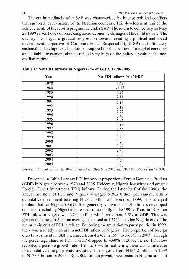
Table 1: Net FDI Inflows in Nigeria (% of GDP) 1970-2005

Year Net FDI Inflows % of GDP

1970 1.631980 -1.151985 1.211990 2.111991 2.151992 2.181993 2.721994 2.481995 2.411996 2.151997 4.251998 3.801999 4.242000 3.572001 4.272002 5.312003 5.632004 3.772005 4.60

Source: Computed from the World Bank Africa Database 2005 and CBN Statistical Bulletin 2005

Presented in Table 1 are net FDI inflows as proportion of gross Domestic Product (GDP) in Nigeria between 1970 and 2005. Evidently, Nigeria has witnessed greater Foreign Direct Investment (FDI) inflows. During the latter half of the 1990s, the annual net flow of FDI into Nigeria averaged N26.2 billion per annum, with a cumulative investment totalling N154.2 billion at the end of 1999. This is equal to about half of Nigeria’s GDP. It is generally known that FDI into less developed countries (including Nigeria) increased substantially in the 1990s. Thus, in 1998, net FDI inflow to Nigeria was N24.1 billion which was about 3.8% of GDP. This was greater than the sub-Saharan average that stood at 1.32%, making Nigeria one of the major recipients of FDI in Africa. Following the transition to party politics in 1999, there was a steady increase in net FDI inflow to Nigeria. The proportion of foreign direct investment in GDP increased from 4.24% in 1999 to 5.63% in 2003. Though the percentage share of FDI in GDP dropped to 4.60% in 2005, the net FDI flow recorded a positive growth rate of about 30%. In real terms, there was an increase in cumulative foreign private investment in Nigeria from N154.2 billion in 1999 to N178.5 billion in 2003. By 2005, foreign private investment in Nigeria stood at

BOJE: Botswana Journal of Economics1�

N269.8 billion, representing about 75% increase from 1999.Figure 2 shows the total inflow of FDI into the Nigerian economy, while Figure 3

shows the origin of the FDI inflows. The last (Figure 4) provides the data according to the sectors that attracted investment flows. Most of the FDI into Nigeria originated from UK, Western Europe and the US. Until the mid-1990s, FDI from the UK dominated the economy. This was followed by FDI from Western Europe. The US accounted for a small proportion of FDI. There was a significant change in the structure and origin of investment in the 1990s, with Western Europe and the US taking over a greater proportion of the FDI inflows in the latter part of the 1990s and in the maiden years of the new millennium (2000-2005).

An examination of the activity sectors that benefited from foreign private investment indicates that mining and quarrying, manufacturing and processing, and trading and business services received the highest amount in a descending order of importance. In the 1970s, the oil boom attracted tremendous FDI in the mining and quarrying sector. The import substitution industrialisation (ISI) strategy also encouraged investment in the manufacturing sector. The oil glut of the late 1970s and early 1980s together with the global economic recession significantly affected the flow of investment into all sectors. Despite the general decline, manufacturing sector benefited from FDI inflows as it accounted for the largest proportion of cumulative FDI for many years between 1978 and 1988. This dominance continued until the early 1990s when the rising share of the mining and quarrying sector again broke it. The dominance of the resource-based sector in attracting FDI is obvious.

Figure 2: Foreign Private investment inflows to Nigeria, 1970-2005

-5000

0

5000

10000

15000

20000

1970 1975 1980 1985 1990 1995 2000 2005

year

N' m

illio

n

FDI

Figure 3: Cumulative Foreign Private Investment By Country of Origin

-20

-10

0

10

20

30

40

50

60

70

80

1965 1970 1975 1980 1985 1990 1995 2000 2005 2010

Year

Perce

ntage

Mine Manuf trading Others


Figure 4: Cumulative Foreign Private Investment in Nigeria by Type of Activity

-100

0

100

200

300

400

500

600

1960 1970 1980 1990 2000 2010

year

percenta

ge

UK USA WE Others

3. Determinants of FDI in Developing CountriesThe flow of FDI to developing countries is influenced by numerous factors. These

factors are not only complex but also interrelated. From the growing literature, the widely discussed determinants can be grouped into two broad categories. These are the ‘push factors’ and the ‘pull factors’. Only a summary discussion of the literature on this theme is presented here.

Push factors. The push factor theory attributes the direction of capital flows to what happens on the international front such as a fall in international interest rates, business cycles in industrial countries and a rise in international diversification (Calvo and Reinhart, 1998 and Calvo, et al, 1996). In addition, increasing tax burdens of multinational corporations in their home countries has also been found to be a key push factor. The upsurge in capital flows to developing countries, particularly in the 1990s, has been attributed to the decline in interest rates in the US (Calvo et al, 1993; Fernandez-Arias, 1994). This development has important implications for the sustainability of foreign investment and hence, policy design. If it is lower interest rate that is the driving force for the upsurge in capital flows to developing countries, it means that a reversal in such rates would threaten the sustainability of capital flows.

Pull factors. The pull factors, on the other hand, trace the causes of capital flows to domestic factors. These include domestic factors such as autonomous increases in domestic money demand and increases in the domestic productivity of capital (Haque, Mathieson and Sharma, 1997), improvement in external creditor relations, adoption of sound fiscal and monetary policies and neighbourhood externalities (Calvo, et al, 1996). Among other domestic factors, macroeconomic performance, the investment environment, infrastructure and resources and the quality of institutions are paramount.

Many scholars have identified domestic economic reforms as the main attraction for capital flows to the developing countries in the 1990s. The core of their argument is that economic reforms in the form of privatisation of public enterprise, liberalisation of currency and capital accounts, coupled with stable macroeconomic environment have improved credit worthiness and expanded investment opportunities (Chuhan et al, 1994 and UI Haque, et al, 1996). Based on the evidence from some African success stories, Basu and Srinivasan (2002) posit that political and macroeconomic stability, well-designed structural reforms, and natural resources contributed to an increase in FDI to these countries. In addition, it has also been found that FDI tends to cluster in certain (particular) locations (the agglomeration effect) (Kamaly, 2002). Thus, FDI flows depend on a country’s past stock of FDI - countries that have been successful in attracting FDI in the past are more likely to do so in the future. In another study, Asiedu (2002) in the quest for explanations behind the small


proportion of FDI flows to African countries found trade restriction and poor policy as the major culprits. African countries tend to be less open than other emerging markets; are perceived as very risky and are characterised by poor policy environment relative to other developing countries. In collaboration with earlier studies, Rogoff and Reinhart (2003) found that high incidence of regional conflicts, high and volatile rates of inflation, and frequent currency crashes play an important role in explaining why African countries lag behind other regions in attracting FDI.

Macroeconomic volatility. FDI, like other forms of investment, also depends on non-economic factors such as risk, macroeconomic volatility and political instability. FDI is a forward-looking activity based on investors’ expectations regarding future returns and the confidence that they can place on these returns. These variables increase uncertainty and discourage investment. For instance, apart from intermittent disruption of production activity political instability in a host country can lead to destruction of the facility of the foreign investors. Fluctuating exchange rates have several disadvantages. First, if price elasticities are low, exchange rate depreciation effects could be perverse. Second, it is usually associated with uncertainty and exchange rate risks. Third, fluctuations in the exchange rate can result in significant reduction in the value of assets invested in the host country as well as the future profits generated by the investment. Lastly, speculation on the future course of exchange rate movements can be destabilising hence, imposing losses in economic efficiency and inducing potentially avoidable capital flights. In this respect, Chakrabarti (2001) reported a negative relationship between exchange rate volatility and FDI flows from the United States to twenty OECD countries.

With respect to African countries, the main factors inhibiting increased inflow of FDI are that most countries are regarded as high risk and are characterised by a lack of political and institutional stability, price instability, high level of corruption and stagnant markets (Rogoff and Reinhart (2003). A stable macroeconomic and political environment is therefore important for FDI because investors require as much certainty as possible about the direction of the economy (Hess, 2000).

Essentially, the review above suggests that apart from the pull and push factors widely acknowledged in the empirical and theoretical literature, macroeconomic volatility plays a key role in the decision of foreign investors to locate new FDI or expand existing ones in a country. However, in general, most of the existing empirical studies neglected this variable. Akinkugbe (2003) is closest in approach to the present study. He found inflation rate not significant in the empirical study of the determinants of FDI inflows to hitherto neglected developing countries. It is not certain whether the same finding would be obtained if inflation rate uncertainty was used instead of inflation rate itself. Though Chakrabarti (2001) reported a negative relationship between exchange rate volatility and FDI flows from the United States to twenty OECD countries, the countries involved in the study are not developing countries. Hence, it is doubtful if the findings obtained would be applicable in the context of a developing country like Nigeria with most of the FDI concentrated in the extractive industry. Whether macroeconomic volatility truly matters as determinant of FDI flow to a developing country is the empirical issue which this study attempts to explore using Nigeria as case study.

4. Some Theoretical IssuesTraditionally, the multiplier-accelerator model states that changes in capital stock or investment are determined mainly by income and interest rate. However, there are other factors that determine investment; these include risk, government policy and expected return or profitability of investment. The determinants of foreign


capital flows are more complicated. Several frameworks exist for analysing the determinants of foreign investment. The principal theoretical inspiration for this study is the portfolio allocation theory attributed to Fedderke (2002). According to the theory, foreign investment flows are determined by two factors; rates of return and risk. While foreign capital flows respond positively to rates of return, it is adversely affected by risk. In developing this model, Fedderke (2002) assume that investors seek to maximize the present value of their utility derived from net expected return on a portfolio of capital assets. Formally, individual investor maximizes the function:

dtRue t )(∫ − r (1)R is the net expected return on a portfolio of investment. It is assumed that there are two forms of investment, domestic and foreign. Gross return on each investment has to be adjusted against the respective transaction costs associated with adjusting each investment to desired level. Hence, R is made up of net return on domestic investment and net return on foreign investment. Let Rd and Rf denote net returns on domestic and foreign investment, respectively, then

cRf FFR −= (2)CRd DDR −= (3)

where DR and FR are expected returns on domestic and foreign investment, respectively; and DC and FC are the costs of adjustment of domestic and foreign investment holdings, respectively. Since foreign investment involves dealing in foreign currency, net expected returns on foreign investment must be weighted by probability of exchange rate fluctuation (in particular exchange rate depreciation). Let π represent the non-zero probability of exchange rate depreciation. Invoking the zero-arbitrage condition, the equilibrium condition can be specified as: df RR =− )1( por

CRCR DDFF −=−− )1)(( p (4)According to this condition, the investor will reach his equilibrium when net expected returns on foreign investment equals the net expected return on domestic investment holdings. In real term, foreign investment will be more attractive if the net expected return on foreign investment weighted by appropriate index of exchange rate fluctuation is greater than the net expected returns on domestic investment. Implicitly, equilibrium level of foreign investment flow associated with this condition (F*) is a function of the project level expected return going to all types of investment, the exchange rate and the adjustment costs. That is,

),,,,(** CCRR FDDFFF p= (5)Totally differentiating equation (5), holding domestic investment adjustment costs constant and approximating the derivatives by first differences gives

pp∆+∆+∆+∆=∆ ***** FFFDFFFF Cc

Rd

Rf (6)

Equation (6) states that short run changes in equilibrium foreign investment flows are due to changes in gross expected returns on foreign investment and domestic investment, adjustment costs associated with foreign investment as well as exchange rate uncertainty. However, returns to both types of investment themselves depend on other factors. Returns on foreign investment are functions of exogenous factors such as foreign interest rates, macroeconomic policies and the health of foreign economies (Schadler, et al. 1993). Returns on domestic investment, on the other hand, depend on such factors as domestic market structure and institutions, anticipated structural

BOJE: Botswana Journal of Economics20

reform, positive short-term macroeconomic policies and openness of the economy (Fernandez-Arias and Montiel, 1996). Studies by Hossain and Chowdhury (1998) and Reisen (1996) have shown that high investment yields, sustained growth as well as maintenance of macroeconomic stability attracted huge foreign investment to East Asian economies, particularly in the mid-80s and 90s.

5. The Model and Data SourcesArising from the empirical literature and theoretical framework above, the basic

model for the analysis is of the form:

(7)

where;

FDIGDP is foreign direct investment inflow over gross domestic product (GDP)RGDP is real growth of GDP TRADE is ratio of the trade to GDP INT is the international interest rate (US treasury bill rate is used as proxy)VOLINF is inflationary volatilityVOLEXC is exchange rate volatilityGCON is general government final consumption (% GDP)POLIST is political instabilityDOMCRGDP is domestic credit to the economy over GDPPHONE is telephones per 1,000 peopleREALINT is real domestic interest rate

The real growth of gross domestic product (GDPG) captures the size of the potential market for the foreign investors’ products. It serves as an index for measuring the level of development in a country and thus reflects the purchasing power of individual consumers. It is also a proxy for the comparative return on investing in different countries. It is believed that as economic growth rate increases, the real return to capital will rise and therefore raise net foreign direct investment. In addition, recent trend in FDI inflow to developing countries have shown that middle-income developing countries accounted for a substantial proportion of the flows relative to the low-income countries (Akinkugbe, 2003). The trade-to-GDP variable measures the openness (international competitiveness) of the country to international trade. A low value of this variable implies high tariff barriers, which would attract horizontal FDI, while a high value would indicate openness to trade, an incentive attractive to foreign investors (Caves, 1996).

The interest rate (INT) is a proxy for cost of capital. According to the neoclassical theory, an increase in the interest rate raises the cost of capital and therefore reduces the incentive to accumulate more capital. Similarly, a decrease in the interest rate reduces the cost of capital and stimulates investment. In respect of foreign investment, a decrease in international interest rate raises the amount of profit from

ma

aaaaa

aaaaaa

+++++−+

++++++=

REALINTDOMCRGDPPOLISTGCONFDIGDPPHONE

VOLEXCVOLINFINTTRADEGDPGFDIGDP

11

109876

543210

)1(

Elijah Udoh & Festus Egwaikhide 21

owning capital even in the foreign country and hence, stimulates foreign investment. In the case of foreign investment, two interest rates are vital to the decision to invest: the international interest rate (or the source-country rate) and the domestic interest rate (REALINT). The international interest rate represents the cost of fund to the foreign investors and is expected to have a negative effect on foreign investment. The real domestic interest rate, on the other hand, serves as an indicator of the rate of return on investment in the host country and it is therefore expected to have a positive effect on foreign direct investment.

The development of infrastructure (proxied by the variable telephones per 1,000 people) is expected to have a positive effect on foreign direct investment. Domestic credit to the private sector (DOMCRGDP) is used as an indicator of financial market development. It is expected to have a positive effect on foreign direct investment. An indicator of the size of government, the level of government final consumption expenditure (GCON), is expected to be positive.

The other additional variables are measures of macroeconomic as well as political instability. Foreign exchange rate volatility increases the uncertainty of demand for the product of export-oriented firms and may reduce the profitability of FDI (Kamaly, 2002). Inflation volatility is another source of uncertainty for foreign investors and is also expected to have adverse effect on FDI. Political instability leads to loss of investment as well as compounds inflation rate uncertainty and exchange rate volatility. Thus, the coefficients of the macroeconomic volatility and political condition variables are expected to be negative.

b. Data Sources and Estimation Techniques The data for this study were gathered from various publications of the Central

Bank of Nigeria including CBN Statistical Bulletin (2005). These were supplemented with data obtained from the World Bank African Database 2005 CD-ROM and World Development Indicator 2005. Prima facie, values for volatility in exchange rate and inflation uncertainty were estimated using the GARCH modelling technique. The estimation was done in two stages. First, the GARCH model was estimated using the relevant lags of the variables concerned. Second, the residuals were obtained. Volatility is captured by the variance of the residuals. A comprehensive set of estimation and testing procedures for GARCH models is available in Eviews 4.1.

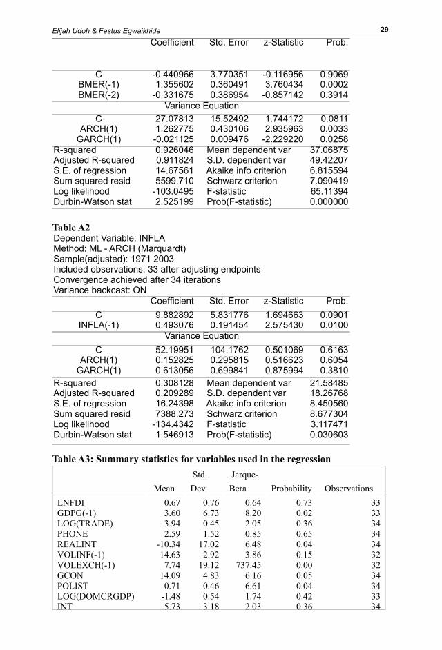
It is believed that the GARCH model can be relied upon to generate good estimates of exchange rate volatility and inflation uncertainty. The test results show that volatility in the exchange rate was not only significant but also persistent in Nigeria over the study period. On the other hand, volatility in inflation rate did not show persistence (see Tables A1 and A2 in the Appendix). As can be seen from Table A1, the sum of the coefficients of ARCH(1) and GARCH(1) is greater than 1, this suggests persistent volatility shocks in foreign exchange rate. However, a similar result could not be obtained in the case of inflation rate whose volatility tends to be less permanent.

BOJE: Botswana Journal of Economics22

6. The Empirical Results Presented in Table A3 (in Appendix) are the summary statistics of the variables

used in the estimation. The summary statistics show that there were wide fluctuations in some variables, namely; exchange rate, inflation rate, and trade openness. Most of the variables also failed the Jarque-Bera normality test.

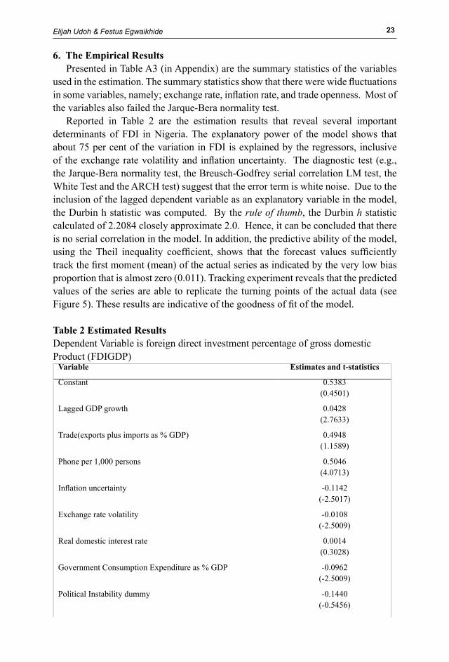
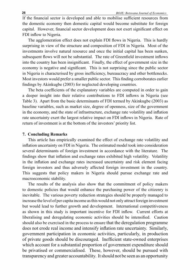
Reported in Table 2 are the estimation results that reveal several important determinants of FDI in Nigeria. The explanatory power of the model shows that about 75 per cent of the variation in FDI is explained by the regressors, inclusive of the exchange rate volatility and inflation uncertainty. The diagnostic test (e.g., the Jarque-Bera normality test, the Breusch-Godfrey serial correlation LM test, the White Test and the ARCH test) suggest that the error term is white noise. Due to the inclusion of the lagged dependent variable as an explanatory variable in the model, the Durbin h statistic was computed. By the rule of thumb, the Durbin h statistic calculated of 2.2084 closely approximate 2.0. Hence, it can be concluded that there is no serial correlation in the model. In addition, the predictive ability of the model, using the Theil inequality coefficient, shows that the forecast values sufficiently track the first moment (mean) of the actual series as indicated by the very low bias proportion that is almost zero (0.011). Tracking experiment reveals that the predicted values of the series are able to replicate the turning points of the actual data (see Figure 5). These results are indicative of the goodness of fit of the model.

Table 2 Estimated ResultsDependent Variable is foreign direct investment percentage of gross domestic Product (FDIGDP)

Variable Estimates and t-statistics

Constant 0.5383(0.4501)

Lagged GDP growth 0.0428(2.7633)

Trade(exports plus imports as % GDP) 0.4948(1.1589)

Phone per 1,000 persons 0.5046(4.0713)

Inflation uncertainty -0.1142(-2.5017)

Exchange rate volatility -0.0108(-2.5009)

Real domestic interest rate 0.0014(0.3028)

Government Consumption Expenditure as % GDP -0.0962(-2.5009)

Political Instability dummy -0.1440(-0.5456)


Domestic credit to the private sector as % GDP (log) -0.0903(-0.5686)

Foreign interest rate (US rate used as proxy) -0.0308(-0.8205)

Lagged foreign direct investment as % GDP (log) 0.0607(0.4002)

R-squared 0.8500Adjusted R-squared 0.7529Durbin-Watson stat 1.5985F-statistic 8.7575

Diagnostic Tests:Jarque-Bera = 1.2364[0.5389]: Test for normality of distribution of residuals (H0: normality)LM Breusch-Godfrey Test = 0.6197[0.5513]: Test for serial autocorrelation of residuals (H0: no autocorrelation)ARCH Test = 0.0262[0.9741]: Test for autocorrelation conditional heteroscedasticity (H0: no heteroscedasticityWhite Test (Xi*Xj) =1.5315[0. 2918]: Test for heteroscedasticity (H0: no Heteroscedasticity)Ramsey RESET = 1.0901[0.3856]: test for general misspecification of equation (H0: no misspecification).

Table 3 Relative Contribution of the FactorsExplanatory Variable Estimated Beta

CoefficientRanking

PHONE 1.0272 1

GCON 0.6555 2

VOLINF 0.4823 3

GDPG 0.3532 4

VOLEXC 0.3047 5

TRADE 0.2997 6

INT 0.1122 7

POLIST 0.0927 8

DOMCRGDP 0.0729 9

FDIGDP(-1) 0.0652 10

REALINT 0.0364 11


-2

-1

0

1

2

3

1975 1980 1985 1990 1995 2000

Actual Predicted

Figure 5: FDI (as % GDP) Forecasts and Actual Elijah Udoh & Festus Egwaikhide

Next are the interpretations of the model results. The effects of both exchange rate volatility and inflation rate uncertainty on FDI in Nigeria are negative. The statistically significant negative coefficient of the exchange rate volatility is not surprising. This is because exchange rate is a price and therefore its movements affect resource allocation in the economy. Thus, when the exchange rate is highly volatile and uncertain, as was the case in Nigeria (especially with the adoption of a market determined exchange rate since September 1986), it hinders the flow of transactions and the movement of financial assets and goods and services. Evidently, this result points to the fact that exchange rate stability is central to the flow of foreign capital into Nigeria. Also, inflation volatility adversely affects FDI, it is statistically significant at the 5 per cent level. A direct import of this is that expansionary macroeconomic policy that raises the inflation rate will deter FDI in Nigeria. The coefficient of the political instability dummy also has negative sign in all the regressions. As expected, the overall impact of the intermittent political unrests in the country over the sample period hindered FDI inflows into the country.

The results in Table 2 further indicate that foreign investors care a great deal about the state of infrastructural facility and the market size in a host economy. The infrastructure variable (PHONE) is positively related to foreign investment and statistically significant even at 1 per cent level of significance. The effect of growth rate of the economy on FDI flow is positive and significant, reinforcing the fact that increasing the rate of economic growth in the country would serve as incentive for FDI inflow.

The coefficient of the foreign interest rate is negative according to prior expectation, though not statistically significant. On the other hand, the effect of domestic interest rate on FDI flow is positive implying that higher real return on investment would encourage FDI flow into the country. However, this variable is not significant. The data on the real interest rate during the period under review show that the country recorded more negative than positive real interest rate. This is due to the regulated interest regime implemented during the period and the high inflation rate made inflation uncertainty more important in investment decision than the interest rate per se.

The results show that the effect of financial sector development proxied by domestic credit to the economy is negative. This is in accordance with the findings of other studies founded on the capital scarcity proposition. This proposition is built around the traditional notion that inadequate domestic capital due to the low saving capacity of developing countries is the main rationale for foreign capital flows.

2�

If the financial sector is developed and able to mobilise sufficient resources from the domestic economy then domestic capital would become substitute for foreign capital. However, financial sector development does not exert significant effect on FDI inflow to Nigeria.

The agglomeration effect does not explain FDI flows in Nigeria. This is hardly surprising in view of the structure and composition of FDI in Nigeria. Most of the investments involve natural resource and once the initial capital has been sunken, subsequent flows will not be substantial. The rate of Greenfield investment inflows into the country has been insignificant. Finally, the effect of government size in the economy is negative and significant. This is not surprising since the public sector in Nigeria is characterised by gross inefficiency, bureaucracy and other bottlenecks. Most investors would prefer a smaller public sector. This finding corroborates earlier findings by Akinkugbe (2003) for neglected developing countries.

The beta coefficients of the explanatory variables are computed in order to gain a deeper insight into their relative contributions to FDI inflows in Nigeria (see Table 3). Apart from the basic determinants of FDI termed by Akinkugbe (2003) as baseline variables, such as market size, degree of openness, size of the government in the economy, and the state of infrastructure, exchange rate volatility and inflation rate uncertainty exert the largest relative impact on FDI inflows in Nigeria. Rate of return of investment is at the bottom of the investors’ priority list.

7. Concluding RemarksThis article has empirically examined the effect of exchange rate volatility and

inflation uncertainty on FDI in Nigeria. The estimated model took into consideration several determinants of foreign investment in accordance with the literature. The findings show that inflation and exchange rates exhibited high volatility. Volatility in the inflation and exchange rates increased uncertainty and risk element facing foreign investors and thus adversely affected foreign investment in the country. This suggests that policy makers in Nigeria should pursue exchange rate and macroeconomic stability.

The results of the analysis also show that the commitment of policy makers to domestic policies that would enhance the purchasing power of the citizenry is inevitable. The various poverty reduction strategies should be properly managed to increase the level of per capita income as this would not only attract foreign investment but would lead to further growth and development. International competitiveness as shown in this study is important incentive for FDI inflow. Current efforts at liberalising and deregulating economic activities should be intensified. Caution should also be exercised in the process to ensure that the deregulation programme does not erode real income and intensify inflation rate uncertainty. Similarly, government participation in economic activities, particularly, in production of private goods should be discouraged. Inefficient state-owned enterprises which account for a substantial proportion of government expenditure should be privatised or commercialised. These, however, should be pursued with transparency and greater accountability. It should not be seen as an opportunity


to further worsen the inequality in the country making the wealthy elites richer and the poor masses poorer.

ReferencesAkinkugbe, O. (2003) “Flow of Foreign Direct Investment to Hitherto Neglected

Developing Countries”, WIDER Discussion Paper No. 2003/02, Helsinki: United Nations University.

Albuquerque, R. (2000) The Composition of International Capital flows: Risk Sharing through Foreign Direct Investment. New York: Cornell University Press.

Andersen, T. G., T. Bollerslev, P. F. Christoffersen and F. X. Diebold (2005) “Volatility Forecasting,” in Elliot, G., C. W. J. Granger and A. Timmermann (eds) Handbook of Economic Forecasting, forthcoming, Amsterdam: North Holland.

Anyanwu, J. C. and E. O. Erhijakpor (2004) “Trends and Determinants of Foreign Direct Investment in Africa”, West African Journal of Monetary and Economic Integration, vol. 4, no. 2, pp. 21-44.

Asiedu, E. (2002), “On the Determinants of Foreign Direct Investment to Developing Countries: Is Africa Different?”, World Development, vol. 30, 107-119.

Basu, A. and Srinivasan, K. (2002), “Foreign Direct Investment in Africa: Some Case Studies”, IMF Working Paper 02/61, IMF, Washington, DC.

Bohn, H and L. L. Tesar (1996), “US Equity Investment in Foreign Markets: Portfolio Rebalancing or Return-Chasing?”, American Economic Review, 86(1).

Bollerslev, T. (1986) “Generalized Autoregressive Conditional Heteroscedasticity”, Journal of Econometrics, Vol. 31, pp. 307-327.

Brada, J. C., A. Kutan and T. Yigit (2004) “The Effects of Transition and Political Instability on Foreign Direct Investment Inflows: Central Europe and the Balkan”, William, Davidson Working Paper No. 729

Calvo, G. A., L. Leiderman and C.M. Reinhart (1993) “Capital Flows and Real Exchange Appreciation in Latin America: The Role of External Factors”, IMF Staff Papers, Vol. 40, No. 1, Washington, DC

Calvo, G. A., L. Leiderman and C.M. Reinhart (1993) “Inflows of Capital to Developing Countries in the 1990s”, The Journal of Economic Perspectives, vol. 10, No. 2 (Spring)

Caves, R. (1996) Multinational Firms and Economic Analysis ( Cambridge University Press) 2nd edition,

Chakrabarti, A. (2001) “The Determinants of Foreign Direct Investment: Sensitivity Analyses of Cross-Country Regressions”, Kyklos, vol. 54, No.1, 89-114.

Chatterjee, P. and Shukayev, M. (2005) “Are Average Growth Rate and Volatility Related?”, University of Minnesota mimeo.

Chuhan, P., S. Claessens and N. Mamingi (1996) “International Capital Flows: Do Short-Term Investment and Direct Investment Differ?” The World Bank, Washington, DC

Chuhan, P., S. Claessens and N. Mamingi (1998) “Equity and Bond Flows to Latin America and Asia: The Role of Global and Country Factors”, Journal of Development Economics, vol. 55(April), 439-63.

Engle, R. F. (1982) “Autoregressive Conditional Heteroscedasticity with Estimates of the Variance of UK Inflation”, Econometrica, vol. 50, 987-1008.

Fedderke, J. W. (2002) “The Virtuous Imperative: Modelling Capital Flows in the Presence of Non-Linearity”, Economic Modelling, vol.19, 445-461.

Fernandez-Arias, E. (1994) “The New Wave of Private Inflows: Push or Pull?”, The Journal of Development Economics, vol. 48, 383-418

Fernandez-Arias, E. and P. J. Montiel (1996), “The Surge in Capital Flows to Developing Countries: An Analytical Overview”, The World Bank Economic Review, vol. 10, No.


1, 51-77.Greene, W. H. (2003) Econometric Analysis ( New York: Prentice Hall), 5th EditionHaynes, S. E. (1998) “Identification of Interest Rates and International Capital Flows”, The

Review of Economics and Statistics, vol. 70, No.1Hernandez, L., and H. Rudolph (1995), “Sustainability of Private Capital Flows to Developing

Countries: Is General Reversal Likely?”, PRE Working Paper, 1518, The World Bank, Washington, DC.

Hess, R. (2000) “Constraints on Foreign Direct Investment”, in C. Jenkins, J. Leape and L. Thomas (eds), Gaining from Trade in southern Africa: complementary Policies to Underpin the SADC Free Trade Area, Macmillan/Commonwealth Secretariat.

Hossain, A. and A. Chowdhury (1998) Open-Economy Macroeconomics for Developing Countries, (Massachusetts: Edward Elgar Publishing).

Johnston, J. and J. Dinardo (1997), Econometric methods, (Singapore: McGraw Hill Int.) 4th Edition,

Kamaly, A. (2002) “Behind the Surge in FDI flows to Developing Countries in the 1990s: an Empirical Investigation”, Unpublished: College Park, Maryland, University of Maryland.

Lastrapes, W. D. (1989) “Exchange Rate Volatility and US Monetary Policy: An ARCH Application,” Journal of Money, Credit and Banking, Vol. 21, 66-77

Maddala, G. S. (2002), Introduction to Econometrics (Wiley Publishers), 3rd EditionMarkusen, J. R., J. R. Melvin, W. H. Kaempfer and K. E. Maskus (1995) International

Trade: Theory and Evidence (Boston: McGraw-Hill).Montiel, P. J. and C. Reinhart (1997) “The Dynamics of Capital Movements to Emerging

Economies during the 1990s”, mimeo William’s College and University of Maryland, prepared for the UNU/WIDER Project on Short-Term Capital Movements and Balance of Payments Crises.

Ndebbio, J. E. U. and A. H. Ekpo (eds.) (1994) The Nigerian Economy at the Crossroads: Policies and their Effectiveness (Calabar: University of Calabar Press).

Reisen, H. (1996) “Managing Volatile Capital Inflows: The Experience of the 1990s”, Asian Development Review, Vol. 14, No.1, 72-96

Rich, R. and J. Tracy (2004) “Uncertainty and Labour Contract Durations”, Review of Economics and Statistics, Vol.86, 270-287.

Rogoff, K. and Reinhart, C. (2003) “FDI to Africa: The Role of Price Stability and Currency Instability”, IMF working Paper 03/10 IMF, Washington, DC.

Schadler, S., M. Carkovic, A. Bennett and R. Khan (1993) “Recent Experiences with Surges in Capital Inflows”, IMF Occasional Paper, 108, IMF, Washington, DC.

Taylor, M. P. and L. Sarno (1997) “Capital Flows to Developing Countries: Long-and Short Term Determinants”, World Bank Economic Review, Vol.11, No.3, Washington, DC.

Ul Haque, N., D. Mathieson and S. Sharma (1997) “Causes of Capital Inflows and Policy Responses to Them”, Finance and Development, Vol. 34, No.1.

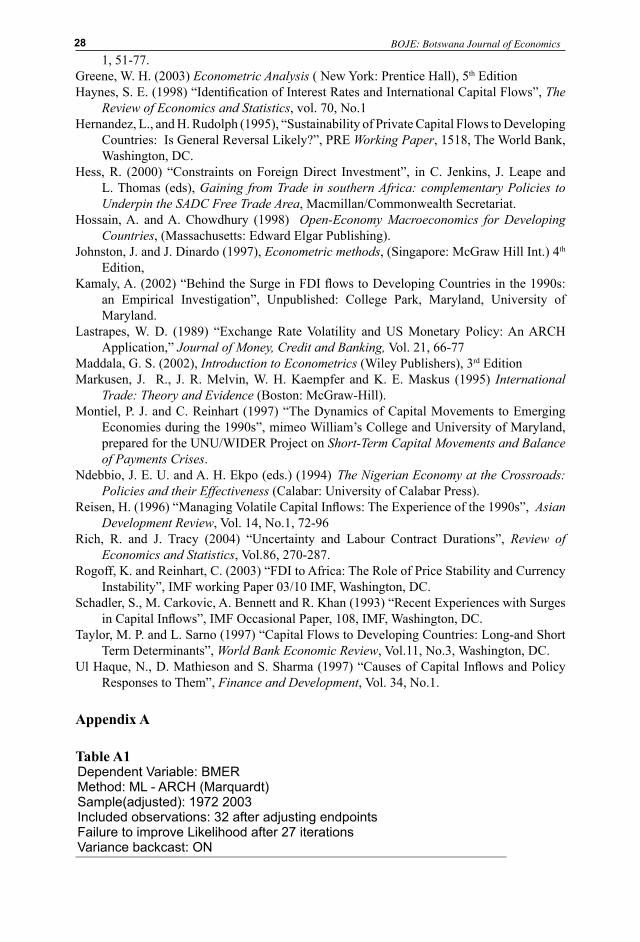
Appendix A

Table A1Dependent Variable: BMERMethod: ML - ARCH (Marquardt)Sample(adjusted): 1972 2003Included observations: 32 after adjusting endpointsFailure to improve Likelihood after 27 iterationsVariance backcast: ON


Coefficient Std. Error z-Statistic Prob.

C -0.440966 3.770351 -0.116956 0.9069BMER(-1) 1.355602 0.360491 3.760434 0.0002BMER(-2) -0.331675 0.386954 -0.857142 0.3914

Variance EquationC 27.07813 15.52492 1.744172 0.0811

ARCH(1) 1.262775 0.430106 2.935963 0.0033GARCH(1) -0.021125 0.009476 -2.229220 0.0258

R-squared 0.926046 Mean dependent var 37.06875Adjusted R-squared 0.911824 S.D. dependent var 49.42207S.E. of regression 14.67561 Akaike info criterion 6.815594Sum squared resid 5599.710 Schwarz criterion 7.090419Log likelihood -103.0495 F-statistic 65.11394Durbin-Watson stat 2.525199 Prob(F-statistic) 0.000000

Table A2Dependent Variable: INFLAMethod: ML - ARCH (Marquardt)Sample(adjusted): 1971 2003Included observations: 33 after adjusting endpointsConvergence achieved after 34 iterationsVariance backcast: ON

Coefficient Std. Error z-Statistic Prob. C 9.882892 5.831776 1.694663 0.0901

INFLA(-1) 0.493076 0.191454 2.575430 0.0100 Variance Equation

C 52.19951 104.1762 0.501069 0.6163ARCH(1) 0.152825 0.295815 0.516623 0.6054

GARCH(1) 0.613056 0.699841 0.875994 0.3810R-squared 0.308128 Mean dependent var 21.58485Adjusted R-squared 0.209289 S.D. dependent var 18.26768S.E. of regression 16.24398 Akaike info criterion 8.450560Sum squared resid 7388.273 Schwarz criterion 8.677304Log likelihood -134.4342 F-statistic 3.117471Durbin-Watson stat 1.546913 Prob(F-statistic) 0.030603

Table A3: Summary statistics for variables used in the regression

Mean Std. Dev.

Jarque-Bera

Probability Observations

LNFDI 0.67 0.76 0.64 0.73 33GDPG(-1) 3.60 6.73 8.20 0.02 33LOG(TRADE) 3.94 0.45 2.05 0.36 34PHONE 2.59 1.52 0.85 0.65 34REALINT -10.34 17.02 6.48 0.04 34VOLINF(-1) 14.63 2.92 3.86 0.15 32VOLEXCH(-1) 7.74 19.12 737.45 0.00 32GCON 14.09 4.83 6.16 0.05 34POLIST 0.71 0.46 6.61 0.04 34LOG(DOMCRGDP) -1.48 0.54 1.74 0.42 33INT 5.73 3.18 2.03 0.36 34


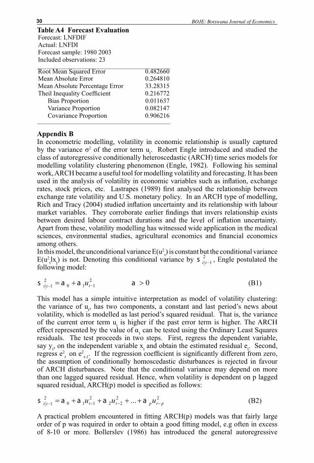
Table A4 Forecast EvaluationForecast: LNFDIFActual: LNFDIForecast sample: 1980 2003Included observations: 23

Root Mean Squared Error 0.482660Mean Absolute Error 0.264810Mean Absolute Percentage Error 33.28315Theil Inequality Coefficient 0.216772 Bias Proportion 0.011637 Variance Proportion 0.082147 Covariance Proportion 0.906216

Appendix BIn econometric modelling, volatility in economic relationship is usually captured by the variance σ2 of the error term ut. Robert Engle introduced and studied the class of autoregressive conditionally heteroscedastic (ARCH) time series models for modelling volatility clustering phenomenon (Engle, 1982). Following his seminal work, ARCH became a useful tool for modelling volatility and forecasting. It has been used in the analysis of volatility in economic variables such as inflation, exchange rates, stock prices, etc. Lastrapes (1989) first analysed the relationship between exchange rate volatility and U.S. monetary policy. In an ARCH type of modelling, Rich and Tracy (2004) studied inflation uncertainty and its relationship with labour market variables. They corroborate earlier findings that invers relationship exists between desired labour contract durations and the level of inflation uncertainty. Apart from these, volatility modelling has witnessed wide application in the medical sciences, environmental studies, agricultural economics and financial economics among others. In this model, the unconditional variance E(u2

t) is constant but the conditional variance E(u2

tlxt) is not. Denoting this conditional variance by 21−tts , Engle postulated the

following model:

2110

21 −− += ttt uaas 0>a (B1)

This model has a simple intuitive interpretation as model of volatility clustering: the variance of ut, has two components, a constant and last period’s news about volatility, which is modelled as last period’s squared residual. That is, the variance of the current error term ut is higher if the past error term is higher. The ARCH effect represented by the value of α1 can be tested using the Ordinary Least Squares residuals. The test proceeds in two steps. First, regress the dependent variable, say yt, on the independent variable xt and obtain the estimated residual et. Second, regress e2

t on e2t-1. If the regression coefficient is significantly different from zero,

the assumption of conditionally homoscedastic disturbances is rejected in favour of ARCH disturbances. Note that the conditional variance may depend on more than one lagged squared residual. Hence, when volatility is dependent on p lagged squared residual, ARCH(p) model is specified as follows:

2222

2110

21 ... ptptttt uuu −−−− ++++= aaaas (B2)

A practical problem encountered in fitting ARCH(p) models was that fairly large order of p was required in order to obtain a good fitting model, e.g often in excess of 8-10 or more. Bollerslev (1986) has introduced the general autoregressive

BOJE: Botswana Journal of Economics�0

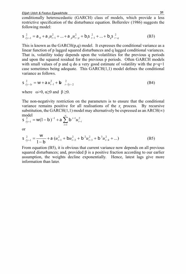
conditionally heteroscedastic (GARCH) class of models, which provide a less restrictive specification of the disturbance equation. Bollerslev (1986) suggests the following model:

2211

22110

21 ...... qtqtptpttt uu −−−−− ++++++= sbsbaaas (B3)

This is known as the GARCH(p,q) model. It expresses the conditional variance as a linear function of p lagged squared disturbances and q lagged conditional variances. That is, volatility today depends upon the volatilities for the previous q periods and upon the squared residual for the previous p periods. Often GARCH models with small values of p and q do a very good estimate of volatility with the p=q=1 case sometimes being adequate. This GARCH(1,1) model defines the conditional variance as follows.

221

21

21 −−−− ++= tttttt u bsaws (B4)

where ω>0, α≥0 and β ≥0.

The non-negativity restriction on the parameters is to ensure that the conditional variance remains positive for all realisations of the zt process. By recursive substitution, the GARCH(1,1) model may alternatively be expressed as an ARCH(∞) model

∑∞

=−

−−− +−=

1

21121 )1(

iit

itt ubabws

or

...)(1

24

323

222

21

21 +++++

−= −−−−− tttttt uuuu bbba

bw

s (B5)

From equation (B5), it is obvious that current variance now depends on all previous squared disturbances; and, provided β is a positive fraction according to our earlier assumption, the weights decline exponentially. Hence, latest lags give more information than later.

Elijah Udoh & Festus Egwaikhide �1

boje: botswana journal of economics volume 5. n exchange

Documents