boehme85

Acoustic backscattering at low grazing angles from the ocean bottom. Part I. Bottom backscattering strength

H. Boehme, N. P. Chotiros, L. D. Rolleigh, S. P. Pitt, A. L. Garcia, T. G. Goldsberry, and R.A. Lamb

Applied Research Laboratorie• The Universit• of Texas at Austin, P.O. Box 8029, Austin, Texas 78713-8029

(Received 21 June 1984; accepted for publication 2 October 1984}

Acoustic backscattering measurements on a sand bottom were made at grazing angles in the range of about 2•-10 ø in water depth of approximately 15.5 m near San Diego, California {reported by T. G. Goldsberry, S. P. Pitt, and R. A. Lamb, 104th Meeting of the Acoustical Society of America, Orlando, FL, 8--12 November 1982). Data from these measurements have been analyzed to determine the mean value and standard deviation of the bottom backscattering strength per square meter as a function of grazing angle, insonified area, transmit signal type, and frequency. A curved ray path proportional model and measured sound speed profiles were used to determine grazing angle versus time. The mean value followed Lainbert's law for the range of grazing angles measured and for all frequencies used. No significant differences in mean value were observed when the insonified area and transmit signal type were varied. The observed frequency dependenee of the bottom backscattering strength per square meter falls in the range fromf •.o to f•'• for this relatively fiat, sandy bottom.

PACS numbers: 43.30.Bp, 43.30.Gv, 92.10.Vz, 91.50.Ey

INTRODUCTION

Acoustic bottom backscattering measurements were made in May 1982 about I mi offshore from Mission Beach, California. The measurements were made using transducers mounted on a tripod assembly about 4 m tall that rested on the bottom. The horizontal and vertical orientation of the

transducers were controlled and monitored by test persound on a nearby oceanographic tower. The acoustic measurements were made over a range of grazing angles of 2 •-10 ø and a range of frequencies of 30-95 kHz. Details of the measurement system as well as the bottom backscattering measurements that were made have been presented previously. •

A preliminary objective of the bottom backscattering measurements was to provide data at low grazing angles from which backscattering strength values and reverberation statistics could be extracted. Several comprehensive reviews have been published which include bottom backscattering strength versus grazing angle in the 20-100 kI-Iz frequency range. 2-4 The most notable of these, by MeKinney and Anderson 2 and by Shultz, 3 are almost 20 years old; only a few measurements at grazing angles below 10 ø are included. The more recent review by Bunehuk and Zhitkovskii 4 includes information at low grazing angles. These reviews generally agree that bottom backscattering can be broadly categorized according to bottom composition, such as mud or silt, sand, and rock or gravel. However, relatively large variations within each general bottom type are common, with little or no correlation of bottom backscattering strength with mean particle size within each of the categor- ies. For grazing angles above about 2 ø, backscattering was reported to increase with grazing angle according to'sin t' 0, where 0 is the grazing angle and k is a number between 1 and 2. For sand sediments, backscattering was found by McKin- ney and Anderson • to increase with frequency while Bun-

chuk and Zhitkovskii 4 concluded that backscattering was independent of frequency, or at most only slightly dependent on frequency, for all bottom types.

The acoustic measurements made in shallow water near

San Diego were specifically planned to provide bottom backscattering data for low grazing angles over a relatively wide range of frequencies. The transmitted pulse waveforms were either cw (pulse lengths of 0.25-25 ms) or linear FM (1-25 ms pulses with 1-4 kHz bandwidths} and were generally transmitted on alternate pings until approximately 75 pings of each pulse type had been transmitted.

Physical oceanographic measurements were made by Naval Ocean Research and Development Activity (NORDA} during the same period of time that acoustic measurements were made. A report on the sediment geoacousti½ properties has been written and distributed?

I. DATA ANALYSIS DESCRIPTION

The acoustic measurement data were recorded on ana-

log magnetic tape records, converted to digital data records by use of general purlx)se analog-to-digital (A/D) eqhip- ment, and processed by use of analysis software written for a general purpose computer (CDC CYBER 171). The digital data record format w_as such that each transmitted pulse and subsequent reverberation period was identified by pulse type, frequency, time, and number of sequential samples composing the digital data record. An envelope was generated for each ping and was then smoothed by time averaging with a moving time window equal in length to the pulse du- ration.

A number of sequential ping cycles (usually 30 to 50) using the same pulse waveform were assembled to form an ensemble. Statistical tests were then performed in order to assure that the assembled envelope records constituted a val-

962 J. Acoust. Soc. Am. 77 (3), March 1985 0001-4966/85/030962-13500.80 ¸ 1985 Acoustical Society of America 962

id ensemble. An existing ray tracing computer program was used to relate time after initiation of the pulse transmission to path length, horizontal range, and grazing angle. A horizontally stratified water column based upon a measured sound speed profile was assumed within the ray tracing computations. A mean backscattering strength and a standard deviation from the mcan were calculated for the ensemble of

envelope data records. The mean backscattering strength BS, in dB/m 2, was

calculated according to the following equation:

BS --- RL -- SL -- 2TL -- 101og[A,D•o(O• •D•v(O 2)], (1)

where

RL = equivalent returned signal level on the hydrophone MRA in dB re: 1 pPa.

SL = acoustic projector on-axis source level in dB re:l pPa at I m,

2TL = two-way propagation loss, in dB, As = effective insonified area, in m 2,

2

Dm{O1) = vertical directivity function of the projector intensity as a function of 0 !. the angular separation bctwcen the maximum response axis (MRA) and the launch angle of the outward ray path, and

D•v(t•z} = vertical directivity function of the hydrophone as a function of 0z. the angular separation between the receive MRA and the termi-

nation angle of the return ray path. Since the returned signal level RL associated with each

path length, range, or grazing angle varies from ping to ping, the power-averaged value was used for backscattering strength computations. Thus, the ensemble average of the square of the envelope was computed and halved, and then the square root taken to obtain RL since narrow-band sig- nals were assumed.

In the assumed horizontally stratified medium with nonuniform sound speed versus depth, the spreading loss portion Ls of the propa•tion loss TL was computed by tracing two rays at slightly different vertical launch angles and determining theft separation at the points of bottom contact. In this manner, a correction factor Cs was determined which arises due to divergence or convergence of the sound rays. The correction factor Cs was the ratio of the actual area insonified perpendicular to the two adjacent rays to the ideal insonified area assuming spherical spreading at the same path length ! and within the same launch angle interval Then, Cs was iven by

Cs = r rd sin 0,/12 0. cos 0,, where

ß = average horizontal range to the points of bottom contact of the two adjacent rays,

rd = difference in horizontal range of the two points, 0, = average grazing angle of the two rays with the bot-

tom,

! = path length along an ideal straight line ray path, 0•d = difference in adjacent ray launch angles, and 0t = average launch angle of two rays with respect to the

horizontal.

HEIGHT ABOVE BO'l-rOM

Ais - Insonified area 8• - (8]•n + 8•n_1)/2

perpendicular to

- e•H0 •

HEIGHT Ol• d ABOVE A x BOTTOM

As BOTTOM

r d ,

A• Imonified area r

A x = Projection of A s rd - rn- rn-1 perpendicular to

FI•. 1. Spreading of rays at path length i, launch angle 0•. (n} Ideal case, (b) practical cas•

The one-way spreading loss Ls in dB was expressed as the ideal spherical spreading loss with the correction factor C s as follows:

L s = -- 20 log l -- 10 log Cs ß (3)

Large numerical values of Cs are indicative of shadow zones while small values are indicative of focusing.

The absorption loss part of the propagation loss was calculated by combining the ray-traced path length and the absorption coefficient (in dB/m), where the absorption coefficient was determined from the Shulkin and Marsh 6 equation. The total one-way propagation loss including absorption loss was expressed as

TL = -- 20 log 1 -- 10 log Cs -- al. (4) Calculation of the effective insonified area also made

use of the ray-tracing computer program. Figure 1 shows sketches of (a) the geometry for ideal (isovelocity) conditions and (b) the geometry used when the medium is assumed to be horizontally stratified with depth-dependent sound speed. When curved ray paths and low grazing angles are appropri- ate, the expression used for the-insonified area is as follows:

A, = o,] , where ß is the horizontal range, •. is the effective horizontal beamwidth of the projector and hydrophone array, Cb is the sound speed just above the bottom, •' is the pulse length, and O s is the grazing angle.

963 J. Acoust. Soc. Am,, Vol. 77, No. 3, March 1985 Boehme et al.: Acoustic backscatter'rig. Part I 963

AMBIENT NOISE SAMPLES

•) •z

u,•

T O T 1 T 2 T 3 RANGE OR TIME •

FIG. 2. Three-dimensional plot of an ensemble of sequential envelope records when propagation conditions were rdatively stable. Transmitted pulsewas0.2$-mscwandeventsontherange/timeaxisare T O: transmit, T. = acoustic target at 70-m range, T2: acoustic target at ] 10-m range, and T 3 = acousfic target at 210-m range.

The effective horizontal beamwidth •r of the projector and hydrophone array is approxitnated in terms of the -- 3 dB horizontal beamwidths of the hydrophone array •h and the l•rojector •, according to the following expression:

•t•1.065(•'2+•-2) -n/z, in radians, (6) where •, and •, are also expressed in radians and the numerical factor arises from an assumption that the mainlobes of the actual hydrophone and projector horizontal directivity functions are approximated by Gaussian functions.

The expression given in Eq. (5) for the insonified area assumes that grazing angle is a constant over the instantan- eous insonified area; this is an acceptable approximation only if the sound speed profile does not result in focusing or shadow zones within the acoustic measurement region of interest. Inaccuracies in grazing angle estimation are propa- gated to esthnates of the inson/fled area.

The acoustic projector on-ax/s source level {$L ) versus transm/t electrical current was determined by acoustic calibration at the Lake Travh Test Station {LTTS) calibration facility prior to making the acoustic backscattering measurements. The transmit current was monitored during the measurements and recorded on data log sheets.

The projector and hydrophone vertical directiv/ty functions were also measured and recorded on data log sheets at LTTS. The vertical direcfiv/ty functions were digitized and stored in a digital calibration data file which could be ac- cessed as needed during the analysis of measurement data.

II. DATA ANALYSIS RESULTS

The acoustic data were analyzed to dete•taine the behavior of bottom backscattering strength as a function of

T O T 1 T 2 T 3 RANGE OR TIME --

FIG. 3. Three-dimensional plot of an ensemble of sequential envelope records when propngation conditions were unstable. Transmitted pulse was 0.25-ms cw and events on the range/time axis are the same as those in Fig. 2.

grazing angle, effective horizontal beamwidth, transmit signal type, frequency, and bottom type. Since backscattering strength was calculated by averaging over an ensemble of envelope records, an attempt was made to select data repre- sentative of the characteristic being investigated over a time interval during which propagation conditions remained relatively stable. In addition to statistical tests used to indicate valid ensembles, three-dimensional plots were generated al- lowing visual indications of the stability of the medium. Fig- ure 2 is an example of such a plot, showing the envelope records of sequential pings of a particular pulse type when propagation conditions were relatively stable. Figure 3 is a similar plot showing unstable propagation conditions as evi- denced by the variation in amplitudes for adjacent ping cycles. The time between pings in both figures was 1 s.

A. Bottom backscattering strength versus grazing angle

Initialestimates ofbackscattering strength were carried out using theoretical estimates of the transducer beam patterns and assuming a constant sound speed versus depth profile. The results obtained were reliable only for ranges less than about 25 m, which corresponded to grazing angles of 10 ø or more. For lower grazing angles and correspondingly longer ranges, the sound speed profile was found to have a significant influence on the results. Examples are shown in Figs. 4 and 5, in which the estimated backscattering strengths as a function of grazing angle are presented. Figure 4 represents estimates based on a constant sound spe•d versus depth assumption, while Fig. 5 represents estimates based on a measured sound speed profile in conjunction with

964 J. Acoust. Soc. ,•m., Vol. 77, No. 3, March 1985 Boehme otal.: AcousMc backscattering. Part I 964

-10 - T - CALIBRATED TARGET

-60 f , I 0 ! 2 3

i I I i i I i

4 5 6 7 8 9 10

GRAZING ANGLE - deg

FIG. 4. An example of backscattering strength estimates as a function of grazing angle where a constant sound sl•ed versus depth was assumed. Frequency

a ray tracing computer program. The results shown in Fig. 4 indicate that grazing angles of 10ø-1 ø were being measured, while those of Fig. 5 indicate that, in reality, the downward refraction caused by the sound speed profile limited the grazing angles to values above about 2.5 ø.

Ray tracing was also used to determine the range, propagation delay, and grazing angle of a few key ray paths, such as the rays at the -- 3 clB points of the vertical beam patterns, and the rays from the center of the mainlobe and the sidelobes. The information was provided in the form of a printout which accompanies the graphical result. Some of this information is illustrated in Fig. 5.. The information is

particularly useful for checking anomalous features in the bottom backscattering strength estimates. Other propagation anomalies, including focusing and shadow zones, are also printed out as warning messages as they are detected.

In order to determine the sensitivity of grazing angle to input sound speed profile, a particular block of data was processed using sound speed profiles measured on two success/re days (:5-6 May) as inputs. The reverberation data used were recorded approximately 2 1/2 h after the sound speed profile was measured on 5 May. A comparison of backscattering strength versus grazing angle is shown in Fig. 6 for input sound speed profiles measured on 5-6 May. Since

-I0-

-40 -

•-50-

0

UPPER -3 dB LIMIT

I

BOOM-U.FACE i i

1 2

T = CALIBRATED TARGET

I UPPER SlOELOBE [ LOWER I HITS SURFACE MAIN LOSE -3 dB LIMIT

3 4 5 6 7 8 9 tO

GRAZING ANGLE - deg

FIG. 5. An example of backscattering strength estimates as a function of grnz- ing angle, with ray tracing and a measured sound speed profile. Frequency

965 J. Acoust. Sec. Am., VoL 77, No. 3, March 1985 goehrne eta/.: Acoustic backscattering. Part I 965

-10 -

== -3o- I

-r I--

z

=•'-4o-

z

n..

•--•. I--

T(b)

o ! 2 3

T{b)

!

1

ii ii ii

LEGEND:

FREQUENCY: 30 kHz

ARRAY: STAVE 5, LF

PULSE: 0.40 ms cw

AZIMUTH: 26.60 ø VERTICAL: -5.0 ø DATE: 5 MAY 1982

TIME: 13:04:57

4 5 6 7 8 9 I0

GRAZING ANGLE - deg

FIG.. 6. An example of backscattering strength v•sus • a•sle estimated b• upon the sam• data set and two different sound speed profile• Curve (a)

input sound speed profile measured proximately 2 h before the acoustic men-

mate8 made with a sound speed profile measured app•x•mntely one day later

the same reverberation data were used for both plots in Fig. 6, the two input sound speed profiles used cause differences of less than 0.5 ø in grazing andes for corresponding bottom features (and calibrated acoustic targets, as indicated).

The bottom backscattering measurements were intend- ed to provide information at grazing angles below about 1 $o. The low grazing angle limit, corresponding to longer ranges, was observed to depend upon the propagation conditions existing at the time the particular backscattering measure- meats were made. In particular, the sound speed profile was such that downward refraction prevented meaningful measurements below about 2 ø, since energy backscattered from the bottom became cont:amipated by energy backscattered from the sea surface at the longer ranges.

The surface reverberation contribution resulted from a

direct stirface path as well as a bottom bounce to surface path with the same two-way travel time as the direct bottom path for bottom backscattering at longer ranges. The sketch in Fig. 7 is helpful in describing the relationship between bottom and surface backscattering. At shorter ranges the bottom-surface and direct surface paths (solid lines) with the same two-way travel time as the direct bottom path are asso-

ciated with the sidelobe region of the projector and receiver vertical beam patterns. The surface reverberation levels are not sufficient to seriously affect the bottom reverberation level. However, at longer ranges, the bottom surface and direct surface paths (dashed lines) are associated with beam pattern regions that are migrating toward the beam MRA. The direct bottom path, conversely, is associated with beam pattern regions that are migrating away from the beam MRA as the range increases. At some range, depending upon existing propagation conditions and sea surface conditions, the surface reverberation level can become compara- ble with or greater than the bottom reverberation Icyel. This condition imposes a lower grazing angle limit on the analyses of bottom backscattering strength.

To confirm that the background noise level associated with low grazing angles was indeed contaminated by surface reverberation, the background levels were first compared with measured ambient noise levels. The observed back-

ground levels were significantly above ambient noise levels and were observed to depend upon transmitted signal pulse length. The observed background level at the longer ranges was also found to be correlated with wind speed. On occa-

SURFACE

BOTTOM

FIG. 7. Cont, mi•t/on at longer ranges of bottom backscatterin• meaattrement• by surface bac•.atterins.

966 d. Acoust. Soc. Am., VoL 77, No. 3, March 1985 Boehrne eta/.: Acoustic backscatter'ng. Part I 966

-10 ÷

o i

FREQUENCY: 45 kHz

T PULSE TYPE: 0 5 mscw

T - RETURNS FROM FLUID-FILLED SPHERES

T

LIMITING GRAZING

ANGLE

GRAZING ANGLE - deg

IO

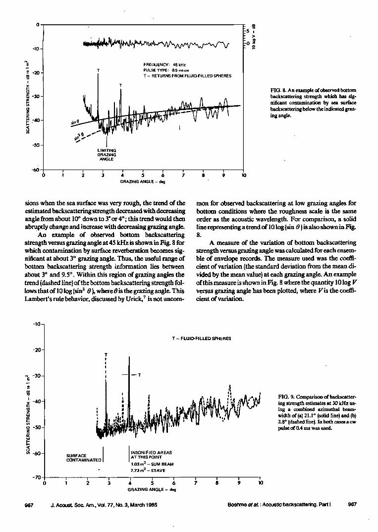
FIG. 8. An example ofob•.Tved bottom backsc•tterin$ strength wMch nificant contnmin=tion by

ing angle.

sions when the sea surface was ve• rough, the trend of the estimated backscattering strength decreased with decreasing angle from about 10 ø down to 3' or 4 ø; this trend would then abruptly change and increase with decreasing grazing angle.

An example of observed bottom backscattering strength versus grazing angle at 45 kHz is shown'in Fig. 8 for which contamination by surface reverberation becomes significant at about 3 ø grazing angle. Thus, the useful range of bottom backscattering strength information lies between about 3 ø and 9.5 ø. Within this region of grazing angles the trend (dashed line) of the bottom backscattering stren•h fol- lowsthat of 10log(sin 2 0), where 0is the grazing angle. This Lambert's rule behavior, discussed by Urick, ? is not uncom-

mon for observed backscattering at low grazing angles for bottom conditions where the roughness scale is the same order as the acoustic wavelength. For comparison, a solid line representing a trend of 10 log (sin 0 } is also shown in Fig. 8.

A measure of the variation of bottom backscattering strength versus grazing .angle was calculated for each ensemble of envelope records. The measure used was the coefficient of variation (the standard deviation from the mean di- vided by the mean value} at each grazing angle. An example of this measure is shown in Fig. 8 where the quantity 10 log V versus grazing angle has been plotted, where Vii the coefficient of variation.

-10-

-70 0

T -- FLUID-FILLED SPHERES

SURFACE I CONTAMINATED

INSONIFIED AREAS AT THIS PONT 1.03 m 2 -- SUM BEAM 7.73 m 2 -- STAVE

2 3 4 5 6

GRAZING ANGLE--d•

I I I I

7 8 9 1o

FIG. 9. Comparison. of backscattering •trength estimates at 30 kHz ing a combined n•imuthal width of(a) 21.1 ø (solid line) and (b) 2.8 ø (ch•hed line). In both cases a cw pulse of 0.4 ms was used.

967 J. Acoust. Soc. Am., Vol. 77, No. 3, March 1985 Boehmo ota/.: Acoustic backscattering. Part I 967

-10-

T

SURFACE CONTAMINATED

T - FLUID-FILLED SPHERES

INSONIFIED AREAS AT THIS POINT

0.92 m 2 - SUM BEAM 6.5 m 2 -- STAVE

-70 I 0 i 2 3 4 5 6 7 8 9

GRAZING ANGLE -cleg

FIG. 10. Comparison of backscattering strength estimates at 45 kl-[z using a combined n•imuthal beamwidth of (a) 14.2 ø {solid line) and (b) 2.0 ø (dashed •ne). In both cases a O.5-ms cw pulse was used.

B. Beamwidth dependence of bottom backscattering strength

Both sum • and 'individual receivin s array stave outputs were recorded during the experiments. Figures 9-13 show comparisons of estimated backscattering strength for the beafnwidths of the sum beams and staves of the receiving arrays for frequencies of 30-95 kHz. The corresponding insonified areas are indicated at a common range point of 70 m on all the figures. For the examples shown, and for other pulse types analyzed, there was no observed dependence of mean bottom backscattering strength on beamwidth. (Minor differences noted in the reverberation statistics are given in

an accompanying paper.) In all cases the variation of the curves from the general trend with grazing angle was notice- ably less for the larger beamwidths associated with the staves than for the beamwidths associated with the sum beams. The

general trend with grazing angle for both stave and sum beam results at all frequencies was observed to follow Lam- bert's rule, as shown in Fig. $.

C. Pulse type dependence

The average bottom backscattering strength versus grazing angle exhibited no dependence upon pulse type or pulse length. Examples of results Obtained using the sum

-I0-

-50 - SURFACE CONTAMINATED


-60 • 0 ! • 3

; j'•' ,.ql•i •V 1;¾ -' • - ,, , 1,•


1.05 m 2 - SUM BEAM 8.1 m 2 - STAVE

I I I I I

4 5 b 7 8

GRAZING ANGLE - deg

I I

9 10

FIG. 11. Comparison of backscattering strength estimates at 60 kHz using a combined n•dmuthal beamwidth of (a• 17.7 ø (•olid Line} and (b) 2.3 ø (dashed line). In both cases a 0.5-ms cw pulse was used.

968 J. Acoust. Soc, Am., Vol. 77, No. 3, March 1985 Boehme et al.: Acoustic backscattering. Part I 968

-10-

SURFACE CONTAM NATED


1.56 m 2 - SUM BEAM 12.1 m 2 - STAVE

-70 i I I [ I I 0 1 2 3 4 5 6

GRAZING ANGLE -- deg


7 8 9 !0

FIG. 12. Comparison of backscattering strength estimates at 80 kHz using a combined azimuthal beamwidth of (a) 13.2 ø (soLid line) • (b) 1.7 ø (c:L•hcd t•_½). In both cases a O.•-ms cw pulse was used.

beam outputs are shown in Figs. 14-18 for frequencies of 30- 95 kHz. In each ease, it can be seen that the bottom backscattering strength associated with each pulse type tended to vary randomly about the same mean value. The results for the FM slide pulse types, with a time-bandwidth product greater than unity, were smoother; all the data have been smoothed by averaging over the pulse length.

D. Frequency dependence

The bottom backscattering strength as a function'of grazing angle was found to fit Lambert's rule fairly well for all frequencies and pulse types used. Therefore the backscattering strength B, may be expressed as

-10 -

B, = 101oBp + 10 log(sin • 0), (7) where 0 = grazing angle and 10 log/t = backscattering strength in dB at normal incidence if Lainbert's rule were valid at nomml incidence.

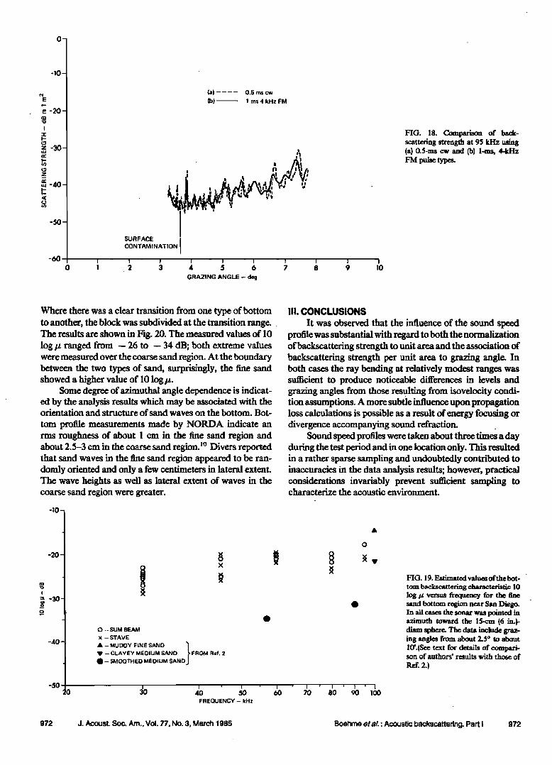
A sin 2 0 function was fitted to each backscattering strength versus grazing angle curve and the value of 101ogH was estimated. The quantity 101ogp was then plotted as a function of frequency; the results are shown in Fig. 19.

Within the particular bottom region for which Fig. 19 applies (fine sand} and over the frequency range considered here, an increase in bottom backscattering strength with frequency was observed. Due to the scatter in the data points, a frequency dependence of 10 logf n, where 1 <n< 1.$, can be

I -r I-

• -40-

z

•_ -5o-

SURFACE CONTAMINATED



1.37 m 2 -- SUM BEAM 10.2 m 2 - STAVE

-•0 I i i i i i ' i 0 1 2 3 4 5 6 7


FIG. 13. Comparison of backscattering strength c•timatca at 95 kHz using a combincd n•m•ltha.! beamwidth of (a) 11.1 ø (solid line) and {b) ].•ø Idashed Une). •n both cases a 0.S-ms cw pulse was used.

i i i

8 9 10

969 J. Acoust. Soc. Am., Vol. 77, No. 3, March 1985 Boehmeetal.:Acou•cbackscattering. Partl 969

-10-

,,z, -40- i=.

z

i,=,

-60 - SURFACE CONTAMINATION

(a) .......... 0.25 ms cw

(b) ....... 0.5 ms cw

(c) .... I ms 4 kHz FM

(d)• 5ms4kHzFM

'70 I I I I I [ I I I ;0 o I 2 3 4 5 6 7 8 9

GRAZING ANGLE - deg

F[O. 14. Compadson of backscattering strength at •0 kHz using (a} 0.25-ms cw, (b) 0.5-ms cw, (½) l- ms, 4-kHz FM, and (d} 5-ms, 4-kl-Iz FM pulse typc•

ß inferred. This frequency dependence is consistent with that reported by McKiuney and Anderson (Ref. 2) of approximately 10 1ogf L6 for field measurements in sand bottom regions. Two points are also shown in Fig. 19 at 100 kHz that were estimated from data below 10 ø grazing angle 2 for sand of about the same particle size as reported in Ref. 5. These points compare very well with data plotted at 95 kHz from the current measurements.

Data reported by Wong and Chesterman s for measurements at low grazing angle in a silty sand region at 48 kHz are 15-20 dB higher than data plotted at 45 kHz from the current measurements. The observed values of 10 1ogp for 30 and 45 kHz shown in Fig. 19 are also substantially lower

than results reported by Crisp et aL 9 at 30 and 48 kHz for two sites in the Puget Sound. No particular frequency dependence was observed in the results from the Puget Sound mca- surements (at 20 ø grazing angl e9).

Bottom backscattering measurements were reported 2 for a water/sand boundary where the sand had been careful- ly smoothed. Values of 10 log/t for grazing angles from about 3ø--10 ø and frequencies of 57 and 90 kHz were deduced from Ref. 2, and are shown in Fig. 19. A straight line through these two points indicates a frequency dependence of 10 log f Le, in good agreement with tl•e current measurements. The level of the backscattering from smooth sand is 10-12 dB below that observed in the current measurements. The high-

-10-

z -40- uJ

z

F- F-

(a) .... 0.5 ms cw

lb)-- lms2kHzFM

-'70 I f i i I I I 'l [ I 0 0 ! 2 3 4 5 6 7 8 9 1


FIG. 15. Comparison of backscattering strength at 45 kI-tz using {a) 0.5-ms cw and (b) 1-ms, 2-kHz FM pulse types.

970 J. Acoust. Soc. Am., VoL 77, No. 3, March 1985 Boehme etat: Acouslic backscattering. Part I 970

-10-

-50-

(a) .......... {3.25 ms cw (b! ....... 0.5 rn• cw (c)-- lms4kHzFM

SURFACE CONTAMINATION

-60- • i I I - I I I I I I 0 1 2 3 4 5 6 7 8 9 !0

GRAZING ANGLE - deg

FIO. 16. Comparison of b•ck- scattering strength at 60 kHz using (a) 0.25-ms cw, (b) 0.5-ms cw, and (c] l-ms, 4-kHz P'M pulse types. [Note: Curves (a) and (c) olXained with ver- ficul tilt angle of -- 3 ø while curve (hi obtained with vertical tilt angle of -- •o.]

er values observed in the current measurements are un-

doubtedly due to the interface relief which was purposely missing in the smooth sand measurements.

E. Azimuth dependence

For the purpose of measuring azimuth dependence, a set of data was taken at 30 kHz in which the sonar beam was

slowly scanned over a large sector of the bottom. The bottom may be separated into two regions--free sand and coarse sand regions•with a discernible boundary between them. s The scan data included measurements in both regions. The sonar beam was tilted vertically at a depression angle of 5 ø. At this depression angie, the bottom reverberation returns

started at a range of about 25 m, at a grazing angle of 10 ø. Unfortunately, due to strong surface activity at the time of the experiment, the bottom backscattering data, beyond a range of about 70 m, were severely contaminated by surface backscatter; therefore only data corresponding to range.• between 25-70 m were used.

The backscatter data appeared to follow Lambert's rule except where there was a transition from one type of sand to another. The data were blocked into nine groups often pings each which, at a scan rate of 1.7 ø between adjacent pings, would correspond to 17 ø sectors. The total sector covered was 153 ø . Within each block, the average Lambert normal incidence backscattering strength 10 log p was estimated.

-10-

-50-

(a} .... 0.5 ms cw

(b) ! ms 2 kHz FM

4 i II

I Ill f

I SURFACE CONTAMINATION

-diDO I I I I r I I [ I I 0 I 2 3 4 5 6 7 8 9 10

GRAZING ANGLE - deg

FIG. 17. Comparison of backscattering strength at 80 kHz using (a) 0.5-ms cw and (b) 1-ms, 2-kHz FM pulse types.

971 J. Acoust. Soc. Am., VOL 77, No. 3, March 1985 Boehrne eta/.: Acoustic backscattering. Part I 971

-10 -

{a! .... 0.5 ms cw

{b}• lms4kHzFM

SURFACE CONTAMINATION

'60 I I I ] I [ o I .2 3 4 5 6


i i I l

7 8 9 I0

FTG. 18. Co• of back- scatterlag streagth at •$ kI• (a) O.$-ms cw and (b) l-ms, FM puhe types.

Where there was a clear transition from one type of bottom to another, the block was subdivided at the transition range. The results are shown in Fig. 20. The measured values of 10 log/z ranged from -- 26 to -- 34 dB; both extreme values were measured over the coarse sand region. At the boundary between the two types of sand, surprisingly, the fine sand showed a higher value of 101ogp.

Some degree of azimuthal angle dependence is indicated by the analysis results which may be associated with the orientation and structure of sand waves on the bottom. Bot-

tom profile measurements made by NORDA indicate an rms roughness of about I cm in the fine sand region and about 2.5-3 cm in the coarse sand region. Iø Divers reported that sand waves in the fine sand region appeared to be randomly oriented and only a few centimeters in lateral extent. The wave heights as well as lateral extent of waves in the coarse sand region were greater.

-10-

-40-

-5O

O -- SUM BEAM

X -- STAVE

ß - MUDDY FINE SAND ß -- CLAYEY MEDIUM SAND •, FROM Ref. 2 ß --SMOOTHED MEDIUM SAND.,)

I I

4O 5O FREQUENCY -- kHz

Ill. CONCLUSIONS

ß It was observed that the influence of the sound speed profile was substantial with regard to both the normalization of backscattering strength to unit area and the association of backscattering strength per unit area to grazing angle. In both cases the ray bending at relatively modest ranges was sufficient to produce noticeable differences in levels and grazing angles from those resulting from isovelocity condition assumptions. A more subtle influence upon propagation loss calculations is possible as a result of energy focusing or divergence accompanying sound refraction.

Sound speed profiles were taken about three time• a day during the test period and in one location only. This resulted in a rather sparse sampling and undoubtedly contributed to inaccuracies in the data analysis results; however, practical considerations invariably prevent sufficient sampling to characterize the acoustic environment.

ß

o

I I I I ' I 60 •0 80 9O tO0

FIG. 19. Estimated value• of the bot-

tom ba•cs•a•g •craoto'i• 1o log/• versus frequency for the free •md bottom regina near San Diego•

azimuth toward the 15-cm {6 in.)- diam sphere. The data include grazing angle• from about 2.5 ø to about 10'.(See text for details of comparison of authors' reaults with those of

972 J. Acoust. Soc. Am., VoL 77, No. 3, March 1985 Boehme oral.: Acoustic backscattering. Part I 972

FINE SAND BOUNDARY COARSE SAND

- 29 dB

- 28 dB

-29 dB

-26dB

FIG. 20. Measured values of Bo from a slow azimuthal scan of the bottom.

Groups of ten pings, which span sectors of 17 ø, w•'e blacked and averaged. The measurements were made at 30 kHz

with a system beamwidth of 2.8 ø. The scanned area covo-ed both fine and

coarse sand regions, with mean grn/n sizes 9 X 10-sin and 5X 10-4 m, respec - tivcly.

N S

BOUNDARY

The lack of an independent measure of propagation loss is believed to have contributed to the scatter of the data at

each frequency. Although fluid-filled spherical acoustic targets were calibrated under free-field conditions and de- ployed in the bottom measurement region, the deployment geometry, environment, and system parameters combined to prevent the use of this information ,to help reduce uncer- tainties in propagation loss. The acoustic targets were very useful as reference points in range and bearing during data acquisition and again during data analyses efforts.

The estimated bottom backscattering strength versus grazing angle plots were often observed to increase with decreasing grazing angle below about 3 ø as has been reported. 2 The observed background levels at the lower grazing angles were found to depend upon pulse length, to be above ambient noise levels, and to correlate with wind speed. The ranges involved when background levels were observed to increase with decreasing grazing angle were consistent with backscattering from the air-water surface. The spatial and tem- poral correlations of data from long ranges and low grazing angles were different from similar correlations at shorter ranges and higher grazing angles. The authors feel that the observed behavior at low grazing angles is a result of energy backscattered from the water surface during these acoustic measurements, and that it is not an anomalous characteristic of bottom backscattering.

The bottom backscattering strength was observed to be independent of beamwidth and pulse lengths at all frequencies used in the acoustic measurements.

The frequency dependence of the bottom backscattering strength over the range of frequencies used was observed to follow a 101ogf n, where n was between I and 1.5. This observed behavior is consistent with results reported in Ref. 2.

An azimuthal dependence was observed in the bottom backscattering strength. The acoustic measurement equip- ment was located near a transition region between fine and coarse sand; data were taken in both regions as the sonar was scanned in azimuth. The highest variability in backscattering strength was observed in the coarse sand region where divers reported larger sand waves than in the fine sand region. Analyses results on bottom roughness are limited at this time; however, the bottom backscattering results observed are expected to be attributable to sand waves and, particularly, to their orientation.

ACKNOWLEDGMENTS

The work was supported by NAVSEA, Code 63R, and NORDA, Code 113. The authors also wish to acknowledge the support of NOSC for the use of the oceanographic tower during the acoustic measurements. We wish also to acknowledge the consultation provided by Dr. John M. Huck- abay, Dr. C. Robert Culbertson, and Garland R. Barnard during all phases of this work, and the efforts provided by Paula Taylor and Delores Higdon in the preparation of the manuscript.

'T. O. Goldsberry, S. P. Pitt, and R. A. Lamb, "Acoustic Backscatter from the Ocean .Bottom," preented at The Acoustical Society of Ame•.a Meeting, Orlando, Florida, 9-12 November 1982. [Copies of this paper are available from ARL:UT and may be obtained by requesting document number ARL-TP-82-46.] ZC. M. McKinney and C. D. Anderson, "Measurements of Backscattering of Sound from the Ocean Bottom," J. Acoust. Soc. Am. 36, 158-163 (1964).

•T. L Schultz, "Undersca Revcrberation (U)," Bolt Beranek and Newman, Rep. 4081255 (December 1965), confidential.

973 J. Acoust. Soc. Am., VoL 77, No. 3, March 1985 Boehme etal.: Acousõc backscattering. Part I 973

4A. V. Bunchult and ¾. Y. Zhitkovskii, "Sound Scattering by the Ocean Bottom in Shallow-Wat• Regions (ReviewL" Soy. Phys. Acoust. 26, 363- 370

SM. D. Richardson, D. K. Yom• and R. I. Ray, "Environmmtal Support for High Frequency Acoustic Measurements at NOSC Oceanographic Tower, 26 April-7 May 1982; Pa•t. I: Sediment Geoacoustic Properties," NORDA Tech. Note 219, Naval Ocean Research and Development Ac- tivity, NSTL Station, Mi•i,•ipl• [tune 1983}.

6H. ScbulUi,• and H. W. Marsh, "Sound Absorption in S•awater." Acousc Soc. Am. 34, 864-S65 {1962}.

•L I. Uri•k, PrinCll•!es of •ndenoager Sound (McCn'aw-Hill, New York,

sH.-I• Wong and W. D. Chesterman, "Bottom Backscattering Near Graz- ing Incidence in Shallow Water,*' I. Acoust. Scc. Am. 44, 1713-1718 0968•

9I. I. Cl'•l• Y. Ii, ara•hi, and D. R. Jackson, "Ftrst Annual Report on •rCP Bottom Scattering Measurements," The Technical Cooperation Program, Subgroup O {June 1980}.

*øM.D. Richsrdson, Naval Ocean Research and Development Activity (p•vate communication}.

974 J. Acoust Soc. Am., Vol. 77, No. 3, March 1985 Boehrne et •.: Acoustic backscattering. Part I 974