block ciphers { focus on the linear layer (feat. · block ciphers { focus on the linear layer...

Block Ciphers – Focus On The Linear Layer(feat. PRIDE)?

Full Version

Martin R. Albrecht1??, Benedikt Driessen2? ? ?, Elif Bilge Kavun3†,Gregor Leander3‡, Christof Paar3, Tolga Yalcın4? ? ?

1 Information Security Group, Royal Holloway, University of London, UK2 Infineon AG, Neubiberg, Germany

3 Horst Gortz Institute for IT Security, Ruhr-Universitat Bochum, Germany4 University of Information Science and Technology, Ohrid, Macedonia

Abstract. The linear layer is a core component in any substitution-permutation network block cipher. Its design significantly influences boththe security and the efficiency of the resulting block cipher. Surprisingly,not many general constructions are known that allow to choose trade-offsbetween security and efficiency. Especially, when compared to Sboxes, itseems that the linear layer is crucially understudied. In this paper, wepropose a general methodology to construct good, sometimes optimal,linear layers allowing for a large variety of trade-offs. We give severalinstances of our construction and on top underline its value by presentinga new block cipher. PRIDE is optimized for 8-bit micro-controllers andsignificantly outperforms all academic solutions both in terms of codesize and cycle count.Keywords: block cipher, linear layer, wide-trail, embedded processors.

1 Introduction

Block ciphers are one of the most prominently used cryptographic primitivesand probably account for the largest portion of data encrypted today. This wasfacilitated by the introduction of Rijndael as the Advanced Encryption Standard(AES) [2], which was a major step forward in the field of block cipher design. Notonly does AES offer strong security, but its structure also inspired many cipherdesigns ever since. One of the merits of AES (and its predecessor SQUARE [20])was demonstrating that a well-chosen linear layer is not only crucial for thesecurity (and efficiency) of a block cipher, but also allows to argue in a simpleand thereby convincing way about its security.

? Corresponding author, [email protected]?? Most of this work was done while the author was at the Technical University of

Denmark? ? ? Most of this work was done while the authors were at Ruhr-Universitat Bochum.

† The research was supported in part by the DFG Research Training Group GRK1817/1.

‡ The research was supported in part by the BMBF Project UNIKOPS (01BY1040).

There are two main design strategies that can be identified for block ciphers:Sbox-based constructions and constructions without Sboxes, most prominentlythose using addition, rotation, and XORs (ARX designs). Furthermore, Sbox-based designs can be split into Feistel-ciphers and substitution-permutation net-works (SPN). Both concepts have been successfully used in practice, the mostprominent example of an SPN cipher being AES and the most prominent Feistel-cipher being the former Data Encryption Standard (DES) [22].

It is also worth mentioning that the concept of SPN has not only been usedin the design of block ciphers but also for designing cryptographic permutations,most prominently for the design of several sponge-based hash functions includingSHA-3 [11]. In SP networks, the round function consists of a non-linear layercomposed of small Sboxes working in parallel on small chunks of the state anda linear layer that mixes those chunks. Thus, designing an SPN block cipheressentially reduces to choosing one (or several) Sboxes and a linear layer.

A lot of research has been devoted to the study of Sboxes. All Sboxes ofsize up to 4 bits have been classified (indeed, more than once – cf. [14,38,48]).Moreover, Sboxes with optimal resistance against differential and linear attackshave been classified up to dimension 5 [17]. In general, several constructions areknown for good and optimal Sboxes in arbitrary dimensions. Starting with thework of Nyberg [45], this has evolved into its own field of research in which thosefunctions are studied in great detail. A nice survey of the main results of thisline of study is provided by Carlet [18].

The situation for the other main design part, the linear layer, is less clear.

1.1 The Linear Layer

For the design of the linear layer, two general approaches can be identified.One still widely-used method is to design the linear layer in a rather ad-hocfashion, without following general design guidelines. While this might lead tovery secure and efficient algorithms (cf. Serpent [3] and SHA-3 as prominentexamples), it is not very satisfactory from a scientific point-of-view. The secondgeneral design strategy is the wide-trail strategy introduced by Daemen in [19](see also [21]). Especially for the security against linear [43] and differential [12]attacks, the wide-trail strategy usually results in simple and strong securityarguments. It is therefore not surprising that this concept has found its way inmany recent designs (e.g. Khazad [9], Anubis [8], Grøstl [27], PHOTON [31],LED [32], PRINCE [16], mCrypton [41] to name but a few). In a nutshell, themain idea of the wide-trail strategy is to link the number of active Sboxes forlinear and differential cryptanalysis to the minimal distance of a certain linearcode associated with the linear layer of the cipher. In turn, choosing a good code(with some additional constraints) results in a large number of active Sboxes.

While the wide-trail strategy does provide a powerful tool for arguing aboutthe security of a cipher, it does not help in actually designing an efficient linearlayer (or the corresponding linear code) with a suitable number of active Sboxes.Here, with the exception of early designs in [19] and later PRINCE and mCryp-ton, most ciphers following the wide-trail strategy simply choose an MDS matrix

as the core component. This might guarantee an (partially) optimal number ofactive Sboxes, but usually comes at the price of a less efficient implementation.The only exception here is that, in the case of MDS matrices, the authors ofPHOTON and LED made the observation that implementing such matrices in aserialized fashion improves hardware-efficiency. This idea was further generalizedin [49,56], and more recently in [5].

It is our belief that, in many cases, it is advantageous to use a near-MDSmatrix (or in general a matrix with a sub-optimal branch number) for the over-all design. Furthermore, it is, in our opinion, utmost surprising that there arevirtually no general constructions or guidelines that would allow an SPN designto benefit from security vs. efficiency trade-offs. This is in particular importantwhen it comes to ciphers where specific performance characteristics are crucial,e.g. in lightweight cryptography.

1.2 The Current State of Lightweight Cryptography

In recent years, the field of lightweight cryptography has attracted a lot of at-tention from the cryptographic community. In particular, designing lightweightblock ciphers has been a very active field for several years now. The dominantmetric according to which the vast majority of lightweight ciphers have been op-timized was and still is the chip area. While this is certainly a valid optimizationobjective, its relevance to real-world applications is limited. Nowadays, there areseveral interesting and strong proposals available that feature a very small areabut simultaneously neglect other, important real-world constraints. Moreover,recent proposals achieve the goal of a small chip area by sacrificing executionspeed to such an extent that even in applications where speed is supposedlyuncritical, the ciphers are getting too slow1.

Note that software solutions, i.e. low-end embedded processors, actually dom-inate the world of embedded systems and dedicated hardware is a comparablysmall fraction. Considering this fact, it is quite puzzling that efficiency on low-cost processors was disregarded for so long. Certainly, there were a few ex-ceptions: Several theoretical and practical studies have already been done inthis field. Practical examples include several proposals for instruction set ex-tensions [40,44,50,39]. Among these, the Intel AES instruction set [33] is themost well-known and practically relevant one. There have also been attemptsto come up with ciphers that are (partially) tailored for low-cost processors[54,53,57,28,10,34]. Of these, execution times of both SEA and ITUbee are ratherhigh, mostly due to the high number of rounds. Furthermore, ITUbee uses 8-bitSboxes, which occupy a vast amount of program memory storage. SPECK, onthe other hand, seems to be an excellent lightweight software cipher in terms ofboth speed and program memory.

It is obvious that there are quite some challenges to be overcome in thisrelatively untouched area of lightweight software cryptography. The softwarecipher for embedded devices of the future should not only be compact in terms

1 See also [37] asking “Is lightweight = light + wait?”

of program memory, but also be relatively fast in execution time. It should clearlybe secure and, preferably, its security should be easily analysed and verified. Thelatter can possibly be achieved by building on conservative structures, which areconventionally costly in software implementation, thereby posing even harderchallenges.

One major component influencing all or at least most of those criteria out-lined above is the linear layer. Thus, it is important to have general constructionsfor linear layers that allow to explore and make optimal use of the possible trade-offs.

1.3 Our Contribution

In this paper, we take steps towards a better understanding of possible trade-offsfor linear layers. After introducing necessary concepts and notation in Section 2,we give a general construction that allows to combine several strong linear map-pings on a few number of bits into a strong linear layer for a larger number ofbits (cf. Section 3). From a coding theory perspective, this construction corre-sponds to a construction known as block-interleaving (see [42], pages 131-132).While this idea is rather simple, its applicability is powerful. Implicitly, a spe-cific instance of our construction is already implemented in AES. Furthermore,special instances of this construction are recently used in [7] and [30].

We illustrate our approach by providing several linear layers with an optimalor almost optimal trade-off between hardware-efficiency and number of activeSboxes in Section 4. Along similar lines, we present a classification of all linearlayers fulfilling the criteria of the block cipher PRINCE in Appendix C. Thoseexamples show in particular that the construction given in Section 3 allowsthe construction of non-equivalent codes even when starting from equivalentones. Secondly, we show that our construction also leads to very strong linearlayers with respect to efficiency on embedded 8-bit micro-controllers. For this, weadopt a search strategy from [55] to find the most efficient linear layer possiblewithin our constraints. We implemented this search on an FPGA platform toovercome the big computational effort involved and to have the advantage ofreconfigurability. Details are described in Section 5.1.

With this, and as a second main contribution of our paper, we make use ofour construction to design a new block cipher named PRIDE that significantlyoutperforms all existing block ciphers of similar key-sizes, with the exception ofSIMON and SPECK [10]. One of the key-points here is that our construction ofstrong linear layers is nicely in line with a bit-sliced implementation of the Sboxlayer. Our cipher is comparable, both in speed and memory size, to the newNSA block ciphers SIMON and SPECK, dedicated for the same platform. Weconclude the paper in Section 6 with some open problems and pressing topics forfurther investigation. Finally, we note that while in this paper we focus on SPNciphers, most of the results translate to the design of Feistel ciphers as well.

2 Notation and Preliminaries

In this section, we fix the basic notation and furthermore recall the ideas of thewide-trail strategy.

We deal with SPN block ciphers where the Sbox layer consist of n Sboxes ofsize b each. Thus the block size of the cipher is n × b. The linear layer will beimplemented by applying k binary matrices in parallel.

We denote by F2 the field with two elements and by Fn2 the n-dimensional

vector space over F2. Note that any finite extension field F2b over F2 can beviewed as the vector space Fb

2 of dimension b. Along these lines, the vector space(F2b)n can be viewed as the (nested) vector space

(Fb2

)n.

Given a vector x = (x1, . . . , xn) ∈(Fb2

)nwhere each xi ∈ Fb

2 we define itsweight2 as

wtb(x) = |{1 ≤ i ≤ n | xi 6= 0}|.

Following [21], given a linear mapping L : (Fb2)n → (Fb

2)n its differentialbranch number is defined as

Bd(L) := min{wtb(x) + wtb(L(x)) | x ∈(Fb2

)n, x 6= 0}.

The cryptographic significance of the branch number is that the branch numbercorresponds to the minimal number of active Sboxes in any two consecutiverounds. Here an Sbox is called active if it gets a non-zero input difference in itsinput.

Given an upper bound p on the differential probability for a single Sboxalong with a lower bound of active Sboxes immediately allows to deduce anupper bound for any differential characteristic3 using

average probability for any non-trivial characteristic ≤ p#active Sboxes.

For linear cryptanalysis, the linear branch number is defined as

Bl(L) := min{wtb(x) + wtb(L∗(x)) | x ∈

(Fb2

)n, x 6= 0}

where L∗ is the adjoint linear mapping. That is, with respect to the standardinner product, L∗ corresponds to the transposed matrix of L.

In terms of correlation (cf., for example, [19]), an upper bound c on theabsolute value of the correlation for a single Sbox results in a bound for anylinear trail (or linear characteristic, linear path) via

absolute correlation for a trail ≤ c#active Sboxes.

The differential branch number corresponds to the minimal distance of theF2-linear code C over Fb

2 with generator matrix

G = [I | LT ]

2 Of course(Fb2

)nis isomorphic to Fnb

2 , but the weight is defined differently on each.3 Averaging over all keys, assuming independent round keys.

where I is the n × n identity matrix. The length of the code is 2n and itsdimension is n (here dimension corresponds to log2b(|C|) as it is not necessarilya linear code). Thus, C is a (2n, 2n) additive code over Fb

2 with minimal distanced = Bd(L).

The linear branch number corresponds in the same way to the minimal dis-tance of the F2-linear code C⊥ with generator matrix

G∗ = [L | I].

Note that C⊥ is the dual code of C and in general the minimal distances of C⊥

and C do not need to be identical.Finally, given linear maps L1 and L2, we denote by L1 × L2 the direct sum

of the mappings, i.e.

(L1 × L2)(x, y) := (L1(x), L2(y)).

3 The Interleaving Construction

Following the wide-trail strategy, we construct linear layers by constructing a(2n, 2n) additive codes with minimal distance d over Fb

2. The code needs to havea generator matrix G in standard form, i.e.

G = [I | LT ]

where the submatrix L is invertible, and corresponds to the linear layer we areusing.

Hence, the main question is how to construct “efficient” matrices L with agiven branch number. Our construction allows to combine small matrices intobigger ones. We hereby drastically reduce the search-space of possible linearlayers. This in turn makes it possible to construct efficient linear layers for varioustrade-offs, as demonstrated in the following sections.

As mentioned above, the construction described in [21] can be seen as aspecial case of our construction. The main difference (except the generalization)is that we shift the focus of the construction in [21] from the 4 round super-boxview to a 2 round-view. While Daemen and Rijmen focused on the bounds for 4rounds, we make use of their ideas to actually construct linear layers. Moreover, aparticular instance of the general construction we elaborate on here, was alreadyused in the linear layer of the hash function Whirlwind [7]. There, several smallMDS matrices are used to construct a larger one.

We give a simple illustrative example of our approach in Appendix A.

3.1 The General Construction

We are now ready to give a formal description of our approach. First define thefollowing isomorphism

Pnb1,...bk

:(Fb12 × Fb2

2 × · · · × Fbk2

)n→(Fb12

)n×(Fb22

)n× · · · ×

(Fbk2

)n(x1, . . . , xn) 7→

((x(1)1 , . . . , x(1)

n

), . . . ,

(x(k)1 , . . . , x(k)

n

))

where xi =(x(1)i , . . . , x

(k)i

)with x

(j)i ∈ Fbj

2 .

This isomorphism performs the transformation of mapping Sbox outputs to oursmall linear layers Li. For example, in Appendix A, we considered individualbits (i.e. b1, . . . , bk = 1) from 4 (i.e., k = 4) 4-bit Sboxes (i.e n = 4).

Note that, for our purpose, there are in fact many possible choices for P . Inparticular, we may permute the entries within (Fbi

2 )n. Given this isomorphismwe can now state our main theorem. The construction of P follows the idea of adiffusion-optimal mapping as defined in [21, Definition 5].

Theorem 1. Let Gi = [I | LTi ] be the generator matrix for an F2-linear (2n, 2n)

code with minimal distance di over Fbi2 for 0 ≤ i < k. Then the matrix G =

[I | LT ] with

L =(Pnb1,...bk

)−1 ◦ (L0 × L1 × · · · × Lk−1) ◦ Pnb1,...bk

is the generator matrix of an F2-linear (2n, 2n) code with minimal distance dover Fb

2 where

d = mini

di and b =∑i

bi.

Proof. Since Pnb1,...bk

and(Pnb1,...bk

)−1are permutation matrices, by construction

L has full rank. To see that wtb(w) + wtb(v) ≥ mini di for any v ∈ Fb2 \ {0} and

w = L · v, observe that wtb(w) + wtb(v) is minimal when all entries in v are zeroexcept those mapped to the positions acted on by Lj where Lj is the matrixwith the minimal branch number. ut

Remark 1. The interleaving construction allows to construct non-equivalent codeseven when starting with equivalent Li’s. This is shown in a particular case in Ap-pendix C, where different choices of (equivalent) Li’s lead to different numbersof minimum-weight codewords.

A special case of the construction above is implicitly already used in AES.In the case of AES, it is used to construct a [8, 4, 5] code over F32

2 from 4 copiesof the [8, 4, 5] code over F8

2 given by the MixColumn operation. In the Superboxview on AES, the ShiftRows operation plays the role of the mapping P (and itsinverse) and MixColumns corresponds to the mappings Li.

4

In the following, we use this construction to design efficient linear layers.Besides the differential and linear branch number, we hereby focus mainly onthree criteria:

– Maximize the diffusion (cf. Section 3.3)– Minimize the density of the matrix (cf. Section 4)

4 Note that the cipher PRINCE implicitly uses the construction twice. Once for gen-erating the matrix M as in Appendix A and second for the improved bound on 4rounds, just like in AES.

– Software-efficiency (cf. Section 5)

The strategy we employ is as follows. We first find candidates for L0, i.e.,(2n, 2n) additive codes with minimal distance d0 over F2b0 . In this stage, weensure that the branch number is d0 and our efficiency constraints are satisfied.We then apply permutations to L0 to produce Li for i > 0. This stage maximizesdiffusion.

3.2 Searching for L0

The following lemma (which is a rather straightforward generalization of Theo-rem 4 in [56]) gives a necessary and sufficient condition that a given matrix Lhas branch number d over Fb

2.

Lemma 1. Let L be a bn× bn binary matrix, decomposed into b× b submatricesLi,j.

L =

L0,0 L0,1 . . . L0,n−1L1,0 L1,1 . . . L1,n−1

......

. . ....

Ln−1,0 Ln−1,1 . . . Ln−1,n−1

(1)

Then, L has differential branch number d over Fb2 if and only if all i×(n−d+i+1)

block submatrices of L have full rank for 1 ≤ i < d− 1. Moreover, L has linearbranch number d if and only if all (n− d+ i+ 1)× i block submatrices of L havefull rank for 1 ≤ i < d− 1.

Based on Lemma 1 we may instantiate various search algorithms which wewill describe in Section 4 and Section 5. In our search we focus on cyclic ma-trices, i.e. matrices where row i > 0 is constructed by cyclic shifting row 0 byi indices. These matrices have the advantage of being efficient both in softwareand hardware. Furthermore, since these matrices are symmetric, considering thedual code C⊥ to C = [I | LT ] is straightforward.

3.3 Ensuring High Dependency

In this section, we assume we are given a matrix L0 and wish to construct

L1, . . . , Lk−1 that maximize the diffusion of the map L =(Pnb1,...bk

)−1◦ (L0 ×

L1 × · · · × Lk−1) ◦ Pnb1,...bk

.Given an bn × bn binary matrix L decomposed as in Eq. (1), we define its

support as the n× n binary matrix Supp(L) where

Supp(L)i,j =

{1 if Li,j 6= 00 else

Now assume that Supp(L0) has a zero entry at index i′, j′. If we apply the sameLi in all k positions this means that the outputs from the i′th Sbox have no

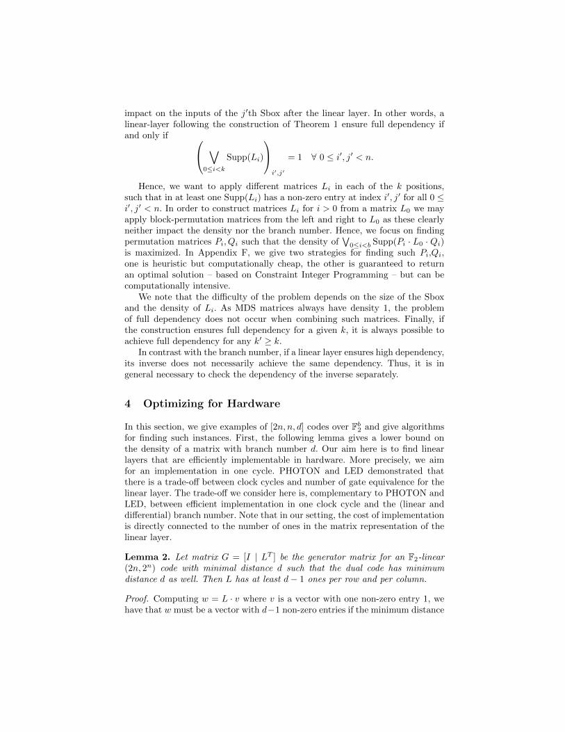
impact on the inputs of the j′th Sbox after the linear layer. In other words, alinear-layer following the construction of Theorem 1 ensure full dependency ifand only if ∨

0≤i<k

Supp(Li)

i′,j′

= 1 ∀ 0 ≤ i′, j′ < n.

Hence, we want to apply different matrices Li in each of the k positions,such that in at least one Supp(Li) has a non-zero entry at index i′, j′ for all 0 ≤i′, j′ < n. In order to construct matrices Li for i > 0 from a matrix L0 we mayapply block-permutation matrices from the left and right to L0 as these clearlyneither impact the density nor the branch number. Hence, we focus on findingpermutation matrices Pi, Qi such that the density of

∨0≤i<b Supp(Pi · L0 · Qi)

is maximized. In Appendix F, we give two strategies for finding such Pi,Qi,one is heuristic but computationally cheap, the other is guaranteed to returnan optimal solution – based on Constraint Integer Programming – but can becomputationally intensive.

We note that the difficulty of the problem depends on the size of the Sboxand the density of Li. As MDS matrices always have density 1, the problemof full dependency does not occur when combining such matrices. Finally, ifthe construction ensures full dependency for a given k, it is always possible toachieve full dependency for any k′ ≥ k.

In contrast with the branch number, if a linear layer ensures high dependency,its inverse does not necessarily achieve the same dependency. Thus, it is ingeneral necessary to check the dependency of the inverse separately.

4 Optimizing for Hardware

In this section, we give examples of [2n, n, d] codes over Fb2 and give algorithms

for finding such instances. First, the following lemma gives a lower bound onthe density of a matrix with branch number d. Our aim here is to find linearlayers that are efficiently implementable in hardware. More precisely, we aimfor an implementation in one cycle. PHOTON and LED demonstrated thatthere is a trade-off between clock cycles and number of gate equivalence for thelinear layer. The trade-off we consider here is, complementary to PHOTON andLED, between efficient implementation in one clock cycle and the (linear anddifferential) branch number. Note that in our setting, the cost of implementationis directly connected to the number of ones in the matrix representation of thelinear layer.

Lemma 2. Let matrix G = [I | LT ] be the generator matrix for an F2-linear(2n, 2n) code with minimal distance d such that the dual code has minimumdistance d as well. Then L has at least d− 1 ones per row and per column.

Proof. Computing w = L · v where v is a vector with one non-zero entry 1, wehave that w must be a vector with d−1 non-zero entries if the minimum distance

of [I | LT ] is d. Hence, there must be at least d− 1 ones per row. Applying thesame argument to w = LT ·v = v ·L shows that at least d−1 entries per columnmust be non-zero. ut

The main merit of the above lemma is that it allows to determine the opti-mal solutions in terms of efficiency. This is in contrast to the case for softwareimplementation, where the optimal solution is unknown.

Lemmas 1 and 2 give rise to various search strategies for finding (2n, 2n)additive codes with minimal distance d over Fb

2. We discuss those strategies inAppendix B and present results of those strategies next.

4.1 Hardware-Optimal Examples

Below we give some examples for our construction. We hereby focus on [2n, n, d]codes over F2, i.e. we use bi = 1.5 Note that this naturally limits the achievablebranch number. For binary linear codes the optimal minimal distance is knownfor small length (cf. [29] for more information). We give a small abridgement ofthe known bounds on the minimal distance for linear [2n, n] codes over F2,F4,and F8 in Appendix E. As can be seen in this table, in order to achieve a highbranch number, it might be necessary to consider linear codes over F2m , or (moregeneral) additive codes over Fm

2 for some small m > 1.

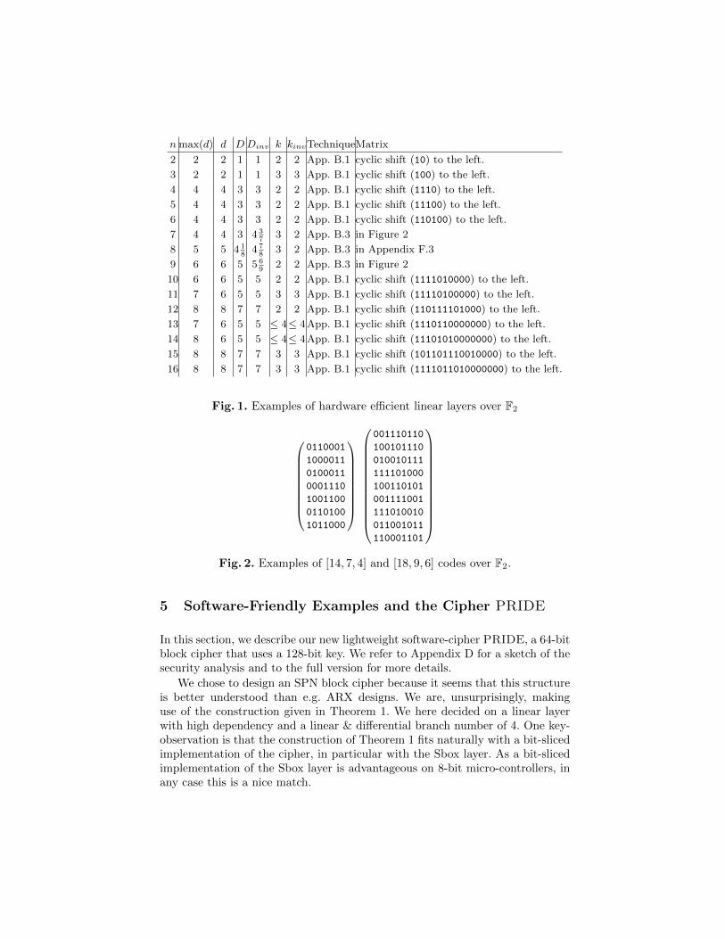
The examples in Figure 1 are optimal in the sense that they achieve the bestpossible branch number (both linear and differential) for the given length (withthe exception of n = 11, 13, and 14) with the least possible number of ones inthe matrix (cf. Lemma 2). The number D corresponds to the average number ofones per row/column and Dinv to the average number of ones per row/columnof the inverse matrix. The only candidate which does not satisfy D = d − 1 isn = 8. This candidate was found using the approach from Appendix B.3, whichguarantees to return the optimal solution. Hence, we conclude that 4 1

8 is indeedthe lowest density possible. That is, there is no 8× 8 binary matrix with branchnumber 5 with only 32 ones, but the best we can do is 33 ones.

For each example we list the dimension (i.e the number of Sboxes), theachieved branch number and the minimal k such that it is possible to achieve fulldependency with two Sbox layers interleaved with one linear layer. These valueswere found using the CIP approach in Section 3.3. Note that in this case (i.e.bi = 1) the value k actually corresponds to the minimal Sbox size that allowsfull dependency. Finally, kinv is the minimum Sbox size to achieve full diffusionfor the inverse matrix. Note that for all these examples, the corresponding codeis actually equivalent to its dual. In particular this implies that the linear anddifferential branch number are equal.

5 We refer to Appendix C for an exemplary comparison of the set of linear layersconstructed by Theorem 1 and the entire space with the same criteria for [8, 4, 4]codes over F4

2.

n max(d) d DDinv k kinvTechniqueMatrix

2 2 2 1 1 2 2 App. B.1 cyclic shift (10) to the left.





7 4 4 3 4 37

3 2 App. B.3 in Figure 2

8 5 5 4 18

4 78

3 2 App. B.3 in Appendix F.3

9 6 6 5 5 69

2 2 App. B.3 in Figure 2




13 7 6 5 5 ≤ 4≤ 4 App. B.1 cyclic shift (1110110000000) to the left.

14 8 6 5 5 ≤ 4≤ 4 App. B.1 cyclic shift (11101010000000) to the left.



Fig. 1. Examples of hardware efficient linear layers over F2

0110001

1000011

0100011

0001110

1001100

0110100

1011000

001110110

100101110

010010111

111101000

100110101

001111001

111010010

011001011

110001101

Fig. 2. Examples of [14, 7, 4] and [18, 9, 6] codes over F2.

5 Software-Friendly Examples and the Cipher PRIDE

In this section, we describe our new lightweight software-cipher PRIDE, a 64-bitblock cipher that uses a 128-bit key. We refer to Appendix D for a sketch of thesecurity analysis and to the full version for more details.

We chose to design an SPN block cipher because it seems that this structureis better understood than e.g. ARX designs. We are, unsurprisingly, makinguse of the construction given in Theorem 1. We here decided on a linear layerwith high dependency and a linear & differential branch number of 4. One key-observation is that the construction of Theorem 1 fits naturally with a bit-slicedimplementation of the cipher, in particular with the Sbox layer. As a bit-slicedimplementation of the Sbox layer is advantageous on 8-bit micro-controllers, inany case this is a nice match.

The target platform of PRIDE is Atmel’s AVR micro-controller [4], as itis dominating the market along with PIC [46] (see [47]). Furthermore, manyimplementations in literature are also implemented in AVR, we therefore opt forthis platform to provide a better comparison to other ciphers (including SIMONand SPECK [10]). However, the reconfigurable nature of our search architecture(cf. Section 5.1) to find the basic layers of the cipher allows us to extend thesearch to various platforms in the future.

5.1 The Search for The Linear Layer

A natural choice in terms of Theorem 1 is to choose k = 4 and b1 = b2 = b3 =b4 = 1. Thus, the task reduces to find four 16× 16 matrices forming one 64× 64matrix (to permute the whole state) of the following form:

L0 0 0 00 L1 0 00 0 L2 00 0 0 L3

Each of these four 16×16 matrices should provide branch number 4 and togetherachieve high dependency with the least possible number of instructions. Insteadof searching for an efficient implementation for a given matrix, we decided tosearch for the most efficient solution fulfilling our criteria.

To find such matrices (Li) that could be implemented very efficiently giventhe AVR instruction set, we performed an extensive and hardware-aided treesearch. Our search engine was optimized to look for AVR assembly code seg-ments utilizing a limited set of instructions that would result in linear behaviourat matrix level. These are namely CLC, EOR, MOV, MOVW, CLR, SWAP,ASR, ROR, ROL, LSR, and LSL instructions. As we are looking for 16 × 16matrices, the state to be multiplied with each Li is stored in two 8-bit registers,which we call X and Y . We also allowed utilization of four temporary regis-ters, namely T0, T1, T2, and T3. We designed and optimized our search engineaccording to these registers. Our search engine checks the resulting matrix Li

after N instructions to see if it provides the desired characteristics. While tryingto reach instruction N , we try all possible instruction-register combinations ineach step. This of course comes with an impractical time complexity, especiallywhen N is increased further. To deal with this time complexity, we came upwith several optimizations. As a first step, we limited the utilization of certaininstruction-register combinations. For example, we excluded CLC and CLR in-structions from the combinations for the first and last instructions. Also, EORis not considered in the first instruction. Again, for the first and last instruc-tions, SWAP, ASR, ROR, ROL, LSR, and LSL instructions are only used withX and Y . Furthermore, we did not allow temporary registers as the destinationwhile trying MOV and MOVW instructions in the last instruction and X − Yregisters as the destination while trying MOV and MOVW instructions in thefirst instruction.

However, such optimizations were not enough to reduce the time complexity.We therefore applied further optimizations, i.e., when the matrices of all registersdo not give full rank, we stop the search as we know that we cannot find aninvertible linear layer any more.

In the end, we found matrices that fulfil all of our criteria starting from 7instructions.

We implemented our search architecture on a Xilinx ML605 (Virtex-6 FPGA)evaluation board. The reconfigurable nature of the FPGA allowed us to changeeasily between different parameters, i.e. the number of instructions. The detailsof this search engine can be found in [35].

5.2 An Extremely Efficient Linear Layer

As a result of the search explained in Section 5.1, we achieved an extremely effi-cient linear layer. The cheapest solution provided by our search needed 36 cyclesfor the complete linear layer, which is what we opted for. The optimal matricesforming the linear layer are given in the Appendix G. Of these four matrices,L0 and L3 are involutions with the cost of 7 instructions (in turn, clock cycles),while L1 and L2 require 11 and 13 instructions for true and inverse matrices,respectively. The assembly codes are given in Appendix H to show the claimednumber of instructions.

Comparing to linear layers of other SPN-based ciphers clearly demonstratedthe benefit of our approach. Note however, that these comparisons have to betaken with care as not all linear layers operate on the same state size and do notoffer the same security level. The linear layer of the ISO-standard lightweightcipher PRESENT [15] costs 144 cycles (derived from the total cycle count givenin [25]). MixColumns operation of NIST-standard AES6 costs 117 instructions(but 149 cycles because of 3-cycle data load instruction utilizations, as Mix-Columns constants are implemented as look-up table – which means additional256 bytes of memory, too) [6]. Note that ShiftRows operation was merged withthe look-up table of Sbox in this implementation, so we take only MixColumnscost as the linear layer cost. The linear layer of another ISO-standard lightweightcipher CLEFIA [51] (again 128-bit cipher) costs 146 instructions and 668 cycles.Bit-sliced oriented design Serpent (AES finalist, 128-bit cipher) linear layer costs155 instructions and 158 cycles. Other lightweight proposals, KLEIN [28] andmCrypton linear layers cost 104 instructions (100 cycles) and 116 instructions(342 cycles), respectively [24]. Finally, the linear layer cost of PRINCE is 357 in-structions and 524 cycles7, which is even worse than AES. One of the reasons forthis high cost is the non-cyclic 4×4 matrices forming the linear layer. The otherreason is the ShiftRows operation applied on 4-bit state words, which makescoding much more complex than that of AES on an 8-bit micro-controller.

6 It is of course not fair to compare a 128-bit cipher with a 64-bit cipher. However, weprovide AES numbers as a reference due to the fact that it is a widely-used standardcipher and its cost is much better compared to many lightweight ciphers.

7 We implemented this cipher on AVR, as we could not find any AVR implementationsin the literature.

5.3 Sbox Selection

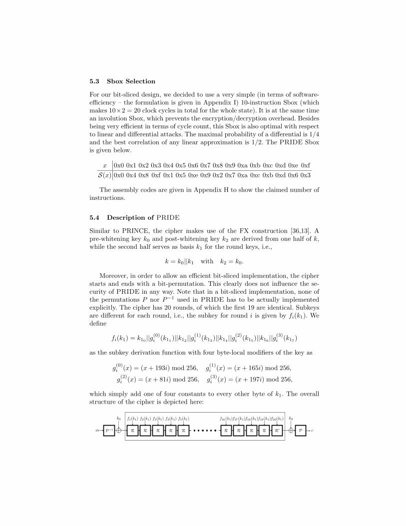
For our bit-sliced design, we decided to use a very simple (in terms of software-efficiency – the formulation is given in Appendix I) 10-instruction Sbox (whichmakes 10×2 = 20 clock cycles in total for the whole state). It is at the same timean involution Sbox, which prevents the encryption/decryption overhead. Besidesbeing very efficient in terms of cycle count, this Sbox is also optimal with respectto linear and differential attacks. The maximal probability of a differential is 1/4and the best correlation of any linear approximation is 1/2. The PRIDE Sboxis given below.

x 0x0 0x1 0x2 0x3 0x4 0x5 0x6 0x7 0x8 0x9 0xa 0xb 0xc 0xd 0xe 0xf

S(x) 0x0 0x4 0x8 0xf 0x1 0x5 0xe 0x9 0x2 0x7 0xa 0xc 0xb 0xd 0x6 0x3

The assembly codes are given in Appendix H to show the claimed number ofinstructions.

5.4 Description of PRIDE

Similar to PRINCE, the cipher makes use of the FX construction [36,13]. Apre-whitening key k0 and post-whitening key k2 are derived from one half of k,while the second half serves as basis k1 for the round keys, i.e.,

k = k0||k1 with k2 = k0.

Moreover, in order to allow an efficient bit-sliced implementation, the cipherstarts and ends with a bit-permutation. This clearly does not influence the se-curity of PRIDE in any way. Note that in a bit-sliced implementation, none ofthe permutations P nor P−1 used in PRIDE has to be actually implementedexplicitly. The cipher has 20 rounds, of which the first 19 are identical. Subkeysare different for each round, i.e., the subkey for round i is given by fi(k1). Wedefine

fi(k1) = k10 ||g(0)i (k11)||k12 ||g

(1)i (k13)||k14 ||g

(2)i (k15)||k16 ||g

(3)i (k17)

as the subkey derivation function with four byte-local modifiers of the key as

g(0)i (x) = (x + 193i) mod 256, g

(1)i (x) = (x + 165i) mod 256,

g(2)i (x) = (x + 81i) mod 256, g

(3)i (x) = (x + 197i) mod 256,

which simply add one of four constants to every other byte of k1. The overallstructure of the cipher is depicted here:

The round functionR of the cipher shows a classical substitution-permutationnetwork: The state is XORed with the round key, fed into 16 parallel 4-bit Sboxesand then permuted and processed by the linear layer.

The difference between R and R′ is that in the latter no more diffusion isnecessary, therefore the last round ends after the substitution layer. With thesoftware-friendly matrices we have found as described above, the linear layer isdefined as follows (cf. Theorem 1 and Appendix G):

L := P−1 ◦ (L0 × L1 × L2 × L3) ◦ P where P := P 161,1,1,1.

The test vectors for the cipher are provided in the Appendix J.

5.5 Performance Analysis

As depicted above, one round of our proposed cipher PRIDE consists of a linearlayer, a substitution layer, a key addition, and a round constant addition (keyupdate). In a software implementation of PRIDE on a micro-controller, we alsoperform branching in each round of the cipher in addition to the previously listedlayers. Adding up all these costs gives us the total implementation cost for oneround of the cipher. The total cost can roughly be calculated by multiplying thenumber of rounds with the cost of each round. Note that we should subtractthe cost of one linear layer from the overall cost, as PRIDE has no linear layerin the last round. The software implementation cost of the round function ofPRIDE on Atmel AVR ATmega8 8-bit micro-controller [4] is presented in thefollowing:

Key

up

dat

e

Key

add

itio

n

Sb

oxL

ayer

Lin

ear

Lay

er

Tot

al

Time (cycles) 4 8 20 36 68

Size (bytes) 8 16 40 72 136

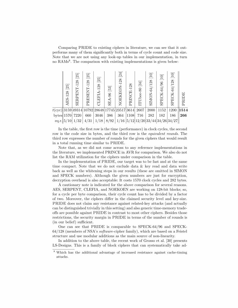
Comparing PRIDE to existing ciphers in literature, we can see that it out-performs many of them significantly both in terms of cycle count and code size.Note that we are not using any look-up tables in our implementation, in turnno RAMs8. The comparison with existing implementations is given below:

AE

S-1

28[2

5]

SE

RP

EN

T-1

28[2

5]

PR

ES

EN

T-1

28[2

5]

CL

EF

IA-1

28[2

5]

SE

A-9

6[5

3]

NO

EK

EO

N-1

28[2

4]

PR

INC

E-1

28

ITU

bee

-80

[34]

SIM

ON

-64/12

8[1

0]

SP

EC

K-6

4/96

[10]

SP

EC

K-6

4/128

[10]

PRID

E

t(cyc) 3159 49314 10792 28648 17745 23517 3614 2607 2000 1152 1200 1514

bytes 1570 7220 660 3046 386 364 1108 716 282 182 186 266

eq.r. 5/10 1/32 4/31 1/18 8/92 1/16 5/12 12/20 33/44 34/26 34/27

In the table, the first row is the time (performance) in clock cycles, the secondrow is the code size in bytes, and the third row is the equivalent rounds. Thethird row expresses the number of rounds for the given ciphers that would resultin a total running time similar to PRIDE.

Note that, as we did not come across to any reference implementations inthe literature, we implemented PRINCE in AVR for comparison. We also do notlist the RAM utilization for the ciphers under comparison in the table.

In the implementation of PRIDE, our target was to be fast and at the sametime compact. Note that we do not exclude data & key read and data writeback as well as the whitening steps in our results (these are omitted in SIMONand SPECK numbers). Although the given numbers are just for encryption,decryption overhead is also acceptable: It costs 1570 clock cycles and 282 bytes.

A cautionary note is indicated for the above comparison for several reasons.AES, SERPENT, CLEFIA, and NOEKOEN are working on 128-bit blocks; so,for a cycle per byte comparison, their cycle count has to be divided by a factorof two. Moreover, the ciphers differ in the claimed security level and key-size.PRIDE does not claim any resistance against related-key attacks (and actuallycan be distinguished trivially in this setting) and also generic time-memory trade-offs are possible against PRIDE in contrast to most other ciphers. Besides thoserestrictions, the security margin in PRIDE in terms of the number of rounds is(in our belief) sufficient.

One can see that PRIDE is comparable to SPECK-64/96 and SPECK-64/128 (members of NSA’s software-cipher family), which are based on a Feistelstructure and use modular additions as the main source of non-linearity.

In addition to the above table, the recent work of Grosso et al. [30] presentsLS-Designs. This is a family of block ciphers that can systematically take ad-

8 Which has the additional advantage of increased resistance against cache-timingattacks.

vantage of bit-slicing in a principled manner. In this paper, the authors makeuse of look-up tables. Therefore, a direct comparison with PRIDE is not fair asthe use of look-up tables does not minimize the linear layer cost. However, tohave an idea, we can try to estimate the cost of the 64-bit case of this family.They suggest two options: The first uses 4-bit Sbox with 16-bit Lbox, and thesecond uses 8-bit Sbox with 8-bit Lbox. The first option has 8 rounds, whichresults in 64 non-linear operations, 128 XORs, and 128 table look-ups in total.The second one has 6 rounds, which takes 72 non-linear operations, 144 XORs,and 48 table look-ups. For linear layer cost, we consider the XOR cost togetherwith table look-ups. Unfortunately, it is not easy to estimate the overall cost ofthe given two options on AVR platform as the table look-ups take more thanone cycle compared to the non-linear and linear operations. Another importantpoint here to mention is that the use of look-up tables result in a huge memoryutilization.

Finally, we note that, despite its target being software implementations,PRIDE is also efficient in hardware. It can be considered a hardware-friendlydesign, due to its cheap linear and Sbox layers.

6 Conclusion

In this work, we have presented a framework for constructing linear layers forblock ciphers which allows to trade security against efficiency. For a given se-curity level, in our case we focused on the branch number, we demonstratedtechniques to find very efficient linear layers satisfying this security level. Us-ing this framework, we presented a family of linear layers that are efficient inhardware. Furthermore, we presented a new cipher PRIDE dedicated for 8-bitmicro-controllers that offers competitive performance due to our new techniquesfor finding linear layers.

One important question is on the optimality of a given construction for alinear layer. In particular, in the case of our construction, the natural ques-tion is if the reduction of the search space excludes optimal solutions and onlysub-optimal solutions remain. For the hardware-friendly examples presented inSection 4 and Appendix C, it is easy to argue that those constructions are opti-mal. Thus, in this case the reduction of the search space clearly did not have anegative influence on the results. In general, and for the linear layer constructedin Section 5 in particular, the situation is less clear. The main reason is that,again, the construction of linear layers is understudied and hence we do nothave enough prior work to answer this question satisfactorily at the moment.Instead we view the PRIDE linear layer as a strong benchmark for efficientlinear layers with the given parameters and encourage researchers to try to beatits performance.

Along these lines, we see this work as a step towards a more rigorous designprocess for linear layers. Our hope is that this framework will be extended infuture. In particular, we would like to mention the following topic for furtherinvestigations. It seems that using an Sbox with a non-trivial branch number

has the potential to significantly increase the number of active Sboxes whencombined with a linear layer based on Theorem 1. Finding ways to easily provesuch a result is worth investigating.

Finally, regarding PRIDE, we obviously encourage further cryptanalysis.

References

1. Tobias Achterberg. Constraint Integer Programming. PhD thesis, TU Berlin, 2007.

2. AES. Advanced Encryption Standard. FIPS PUB 197, Federal Information Pro-cessing Standards Publication, 2001.

3. Ross Anderson, Eli Biham, and Lars Knudsen. Serpent: A Proposal for the Ad-vanced Encryption Standard, 1998.

4. Atmel AVR. ATmega8 Datasheet. http://www.atmel.com/images/doc8159.pdf.

5. Daniel Augot and Matthieu Finiasz. Direct Construction of Recursive MDS Dif-fusion Layers using Shortened BCH Codes. In Fast Software Encryption (FSE),LNCS. Springer, 2014, to appear.

6. AVRAES: The AES block cipher on AVR controllers. http://point-at-infinity.org/avraes/.

7. Paulo S. L. M. Barreto, Ventzislav Nikov, Svetla Nikova, Vincent Rijmen, andElmar Tischhauser. Whirlwind: A New Cryptographic Hash Function. Des. CodesCryptography, 56(2-3):141–162, 2010.

8. Paulo S.L.M. Barreto and Vincent Rijmen. The Anubis Block Cipher. Submissionto the NESSIE project, 2001.

9. Paulo S.L.M. Barreto and Vincent Rijmen. The Khazad Legacy-level Block Cipher.Submission to the NESSIE project, 2001.

10. Ray Beaulieu, Douglas Shors, Jason Smith, Stefan Treatman-Clark, Bryan Weeks,and Louis Wingers. The SIMON and SPECK Families of Lightweight Block Ci-phers. IACR Cryptology ePrint Archive, 2013:414, 2013.

11. Guido Bertoni, Joan Daemen, Michael Peeters, and Gilles Van Assche. KeccakSpecifications, 2009.

12. Eli Biham and Adi Shamir. Differential Cryptanalysis of DES-like Cryptosystems.In CRYPTO, volume 537 of LNCS, pages 2–21. Springer, 1990.

13. Alex Biryukov. DES-X (or DESX). In Encyclopedia of Cryptography and Security(2nd Ed.), page 331. Springer, 2011.

14. Alex Biryukov, Christophe De Canniere, An Braeken, and Bart Preneel. A Toolboxfor Cryptanalysis: Linear and Affine Equivalence Algorithms. In EUROCRYPT,volume 2656 of LNCS, pages 33–50. Springer, 2003.

15. Andrey Bogdanov, Lars R. Knudsen, Gregor Leander, Christof Paar, AxelPoschmann, Matthew J. B. Robshaw, Yannick Seurin, and Charlotte Vikkelsø.PRESENT: An Ultra-Lightweight Block Cipher. In Cryptographic Hardware andEmbedded Systems - CHES 2007, volume 4727 of LNCS, pages 450–466. Springer,2007.

16. Julia Borghoff, Anne Canteaut, Tim Guneysu, Elif Bilge Kavun, MiroslavKnezevic, Lars R. Knudsen, Gregor Leander, Ventzislav Nikov, Christof Paar,Christian Rechberger, Peter Rombouts, Søren S. Thomsen, and Tolga Yalcın.PRINCE - A Low-Latency Block Cipher for Pervasive Computing Applications- Extended Abstract. In ASIACRYPT, volume 7658 of LNCS, pages 208–225.Springer, 2012.

17. Marcus Brinkmann and Gregor Leander. On the Classification of APN FunctionsUp to Dimension Five. Des. Codes Cryptography, 49(1–3):273–288, 2008.

18. Claude Carlet. Boolean Methods and Models, chapter Vectorial Boolean Functionsfor Cryptography. Cambridge University Press, 2010.

19. Joan Daemen. Cipher and Hash Function Design, Strategies Based On Linear andDifferential Cryptanalysis. PhD thesis, Katholieke Universiteit Leuven, 1995.

20. Joan Daemen, Lars Knudsen, and Vincent Rijmen. The Block Cipher SQUARE.In Fast Software Encryption (FSE), LNCS. Springer, 1997.

21. Joan Daemen and Vincent Rijmen. The Wide Trail Design Strategy. In IMA Int.Conf., volume 2260 of LNCS, pages 222–238. Springer, 2001.

22. DES. Data Encryption Standard. FIPS PUB 46, Federal Information ProcessingStandards Publication, 1977.

23. Stefan Dodunekov and Ivan Landgev. On near-MDS codes. Journal of Geometry,54(1):30–43, 1995.

24. Thomas Eisenbarth, Zheng Gong, Tim Guneysu, Stefan Heyse, Sebastiaan In-desteege, Stephanie Kerckhof, Francois Koeune, Tomislav Nad, Thomas Plos,Francesco Regazzoni, Francois-Xavier Standaert, and Loic van Oldeneel tot Olden-zeel. Compact Implementation and Performance Evaluation of Block Ciphersin ATtiny Devices. In AFRICACRYPT, volume 7374 of LNCS, pages 172–187.Springer, 2012.

25. Susanne Engels, Elif Bilge Kavun, Hristina Mihajloska, Christof Paar, and TolgaYalcın. A Non-Linear/Linear Instruction Set Extension for Lightweight BlockCiphers. In ARITH’21: 21st IEEE Symposium on Computer Arithmetics. IEEEComputer Society, 2013.

26. Jean-Charles Faugere. A New Efficient Algorithm for Computing Grobner Basis(F4). Journal of Pure and Applied Algebra, 139(1-3):61–88, 1999.

27. P. Gauravaram, L. Knudsen, K. Matusiewicz, F. Mendel, C. Rechberger,M. Schlaer, and S. Thomsen. Grøstl. SHA-3 Final-round Candidate, 2009.

28. Zheng Gong, Svetla Nikova, and Yee Wei Law. KLEIN: A New Family ofLightweight Block Ciphers. In RFID Security and Privacy (RFIDSec), volume7055 of LNCS, pages 1–18. Springer, 2011.

29. Markus Grassl. Bounds On the Minimum Distance of Linear Codes and QuantumCodes. Online available at http://www.codetables.de , 2007.

30. Vincent Grosso, Gaetan Leurent, Francois-Xavier Standaert, and Kerem Varıcı.LS-Designs: Bitslice Encryption for Efficient Masked Software Implementations.In Fast Software Encryption (FSE), LNCS. Springer, 2014, to appear.

31. Jian Guo, Thomas Peyrin, and Axel Poschmann. The PHOTON Family ofLightweight Hash Functions. In Advances in Cryptology - CRYPTO 2011, vol-ume 6841 of LNCS, pages 222–239. Springer, 2011.

32. Jian Guo, Thomas Peyrin, Axel Poschmann, and Matthew J. B. Robshaw. TheLED Block Cipher. In Cryptographic Hardware and Embedded Systems (CHES),pages 326–341, 2011.

33. Intel. Advanced Encryption Standard Instructions. (Intel AES-NI), 2008.34. Ferhat Karakoc, Huseyin Demirci, and Emre Harmancı. ITUbee: A Software Ori-

ented Lightweight Block Cipher. In Second International Workshop on LightweightCryptography for Security and Privacy (LightSec), 2013.

35. Elif Bilge Kavun, Gregor Leander, and Tolga Yalcın. A Reconfigurable Architecturefor Searching Optimal Software Code to Implement Block Cipher PermutationMatrices. In International Conference on ReConFigurable Computing and FPGAs(ReConFig). IEEE Computer Society, 2013.

http://www.codetables.de

36. Joe Kilian and Phillip Rogaway. How to Protect DES Against Exhaustive KeySearch (An Analysis of DESX). J. Cryptology, 14(1):17–35, 2001.

37. Miroslav Knezevic, Ventzislav Nikov, and Peter Rombouts. Low-Latency Encryp-tion - Is ”Lightweight = Light + Wait”? In CHES, volume 7428 of LNCS, pages426–446. Springer, 2012.

38. Gregor Leander and Axel Poschmann. On the Classification of 4 Bit S-Boxes. InWAIFI, volume 4547 of LNCS, pages 159–176. Springer, 2007.

39. Ruby B. Lee, Murat Fıskıran, Michael Wang, Yedidya Hilewitz, and Yu-YuanChen. PAX: A Cryptographic Processor with Parallel Table Lookup and WordsizeScalability. Princeton University Department of Electrical Engineering TechnicalReport CE-L2007-010, 2007.

40. Ruby B. Lee, Zhijie Shi, and Xiao Yang. Efficient Permutation Instructions forFast Software Cryptography. IEEE Micro, 21(6):56–69, 2001.

41. Chae Lim and Tymur Korkishko. mCrypton – A Lightweight Block Cipher for Se-curity of Low-Cost RFID Tags and Sensors. In Information Security Applications,volume 3786 of LNCS, pages 243–258. Springer, 2006.

42. Shu Lin and Daniel J. Costello, editors. Error Control Coding (2nd Edition).Prentice Hall, 2004.

43. Mitsuru Matsui. Linear Cryptoanalysis Method for DES Cipher. In EUROCRYPT,volume 765 of LNCS, pages 386–397. Springer, 1993.

44. John Patrick McGregor and Ruby B. Lee. Architectural Enhancements for FastSubword Permutations with Repetitions in Cryptographic Applications. In 19thInternational Conference on Computer Design (ICCD 2001), pages 453–461, 2001.

45. Kaisa Nyberg. Differentially Uniform Mappings for Cryptography. In EURO-CRYPT, volume 765 of LNCS, pages 55–64. Springer, 1993.

46. PIC. 12-Bit Core Instruction Set.

47. PIC vs. AVR. http://www.ladyada.net/library/picvsavr.html.

48. Markku-Juhani O. Saarinen. Cryptographic Analysis of All 4 × 4-Bit S-Boxes.In Selected Areas in Cryptography (SAC), volume 7118 of LNCS, pages 118–133.Springer, 2011.

49. Mahdi Sajadieh, Mohammad Dakhilalian, Hamid Mala, and Pouyan Sepehrdad.Recursive Diffusion Layers for Block Ciphers and Hash Functions. In Fast SoftwareEncryption (FSE), volume 7549 of LNCS, pages 385–401. Springer, 2012.

50. Zhijie Jerry Shi, Xiao Yang, and Ruby B. Lee. Alternative Application-SpecificProcessor Architectures for Fast Arbitrary Bit Permutations. IJES, 3(4):219–228,2008.

51. Taizo Shirai, Kyoji Shibutani, Toru Akishita, Shiho Moriai, and Tetsu Iwata. The128-bit Block Cipher CLEFIA (Extended Abstract). In Fast Software Encryption(FSE), volume 4593 of LNCS, pages 181–195. Springer, 2007.

52. Mate Soos. CryptoMiniSat 2.9.6. https://github.com/msoos/cryptominisat, 2013.

53. Francois-Xavier Standaert, Gilles Piret, Neil Gershenfeld, and Jean-JacquesQuisquater. SEA: a Scalable Encryption Algorithm for Small Embedded Applica-tions. In Workshop on Lightweight Crypto, 2005.

54. Tomoyasu Suzaki, Kazuhiko Minematsu, Sumio Morioka, and Eita Kobayashi.TWINE: A Lightweight Block Cipher for Multiple Platforms. In Selected Areas inCryptography (SAC), volume 7707 of LNCS, pages 339–354. Springer, 2012.

55. Markus Ullrich, Christophe De Canniere, Sebastiaan Indesteege, Ozgul Kucuk,Nicky Mouha, and Bart Preneel. Finding Optimal Bitsliced Implementations of4× 4-Bit S-boxes. In Symmetric Key Encryption Workshop, 2011.

56. Shengbao Wu, Mingsheng Wang, and Wenling Wu. Recursive Diffusion Layers for(Lightweight) Block Ciphers and Hash Functions. In Selected Areas in Cryptogra-phy (SAC), volume 7707 of LNCS, pages 355–371. Springer, 2012.

57. Wenling Wu and Lei Zhang. LBlock: A Lightweight Block Cipher. In ACNS,volume 6715 of LNCS, pages 327–344. Springer, 2011.

Appendices

A An Example for the Interleaving Construction

Our example takes its cue from the cipher PRINCE. Assume we want to con-struct a linear layer L working on 4 chunks of 4 bits with linear- and differentialbranch number 4. That is, we want to construct an (8, 24) additive code withminimal distance 4 over F4

2 such that the dual code has minimum distance 4 aswell. As a further requirement in this example, we want to focus on the hardware-efficiency, i.e. we would like to reduce the number of ones in the correspondingmatrix to a minimum. Lastly, we also would like to ensure good diffusion. Moreprecisely, after two Sbox layers interleaved with one linear layer we require thateach bit of the output depends on each bit of the input.

It is not hard to see that (as a matrix) L needs to have at least 3 ones ineach row and column (cf. Lemma 2 in Section 4). We thus face the problem offinding an invertible 16 × 16 binary matrix with branch number 4 and exactly3 ones in each row and column9. As there are 2256 16× 16 matrices, the searchspace is a priori huge.

The basic idea of our construction (depicted below) is simply to first re-groupthe output bits of the Sbox layer.

We collect all first output bits of each Sbox, all second bits, all third bits,and all fourth bits. Next, we apply independently 4 linear mappings on 4 bits,i.e. we multiply each 4-bit chunk with a 4×4 binary matrix. Afterwards the bitsare again re-grouped, and the process is repeated.

The key point (cf. Theorem 1 for the general statement) is that the linear(resp. differential) branch number of the entire linear layer (using wt4) equals theminimal linear (resp. differential) branch number of the 4 small binary matrices(using wt1). Moreover, the number of ones in each row and column in the entirelinear layer is the same as in the small matrices. Thus an optimal solution forthe small binary matrices extends to an optimal solution for the entire linearlayer.

This simple observation allows us to focus on 4×4 binary matrices instead of16×16 matrices. As there are only 216 such matrices (and clearly only 4! of them

9 As a side-note, it is easy to see that no 4×4 matrix over F16 fulfills our requirementsone the number of ones per row and column.

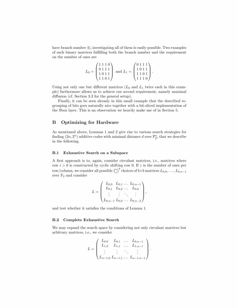
have branch number 4), investigating all of them is easily possible. Two examplesof such binary matrices fulfilling both the branch number and the requirementon the number of ones are

L0 =

1 1 1 00 1 1 11 0 1 11 1 0 1

and L1 =

0 1 1 11 0 1 11 1 0 11 1 1 0

.

Using not only one but different matrices (L0 and L1 twice each in this exam-ple) furthermore allows us to achieve our second requirement, namely maximaldiffusion (cf. Section 3.3 for the general setup).

Finally, it can be seen already in this small example that the described re-grouping of bits goes naturally nice together with a bit-sliced implementation ofthe Sbox layer. This is an observation we heavily make use of in Section 5.

B Optimizing for Hardware

As mentioned above, Lemmas 1 and 2 give rise to various search strategies forfinding (2n, 2n) additive codes with minimal distance d over Fn

2b that we describein the following.

B.1 Exhaustive Search on a Subspace

A first approach is to, again, consider circulant matrices, i.e., matrices whererow i > 0 is constructed by cyclic shifting row 0. If z is the number of ones per

row/column, we consider all possible(nz

)bchoices of b×b matrices L0,0, . . . , L0,n−1

over F2 and consider

L =

L0,0 L0,1 . . . L0,n−1L0,1 L0,2 . . . L0,0

......

. . ....

L0,n−1 L0,0 . . . L0,n−2

,

and test whether it satisfies the conditions of Lemma 1.

B.2 Complete Exhaustive Search

We may expand the search space by considering not only circulant matrices butarbitrary matrices, i.e., we consider

L =

L0,0 L0,1 . . . L0,n−1L1,0 L1,1 . . . L1,n−1

......

. . ....

Ln−1,0 Ln−1,1 . . . Ln−1,n−1

.

and check whether the conditions of Lemma 1 are satisfied. Indeed, the searchspace can be reduced by prunning search trees. This is because of the requirementthat many small submatrices (such as 1 × (n − d)) must have full rank, rulingout many candidates and allowing search trees based on them to be cut.

B.3 System Solving Approaches

Instead of exhaustively searching over (all) possible matrices M to construct(2n, 2n) additive codes with minimal distance d over Fb

2 given by the generatormatrix G = [I | LT ] where L has at most z ones per column and row, we mayexpress the constraints on L as multivariate polynomials or integer constraintsand use off-the-shelf solvers to find matrices satisfying them.

Polynomial System Solving We consider a matrix

L =

L0,0 L0,1 . . . L0,n−1L1,0 L1,1 . . . L1,n−1

......

. . ....

Ln−1,0 Ln−1,1 . . . Ln−1,n−1

with Li,j =

ì,j,0,0 . . . ì,j,0,b−1ì,j,1,0 . . . ì,j,1,b−1

.... . .

...ì,j,b−1,0 . . . ì,j,b−1,b−1

where ì,j,i′,j′ for 0 ≤ i, j < n and 0 ≤ i′, j′ < b are variables over F2. Weconstruct an equation system in the variables ì,j,i′,j′ with equations to enforcethe following three conditions:

1. By Lemma 1 we require that all i × (n − d + i + 1) block submatrices ofL have full rank for 1 ≤ i < d − 1. This is equivalent to requiring thatat least one of the min(i, n − d + i + 1) × min(i, n − d + i + 1) minorsmust have determinant 1. Hence, if t0, . . . , ts represent the determinants ofall min(i, n − d + i + 1) × min(i, n − d + i + 1) minors, we require that

0 =∏s−1

i=0 (ti + 1).

2. We require that L has full rank by requiring that det(L) = 1 is one.

3. Given a target number of ones per row/column z, we require that any prod-uct of z + 1 variables in one row/column is zero.

We may then use any polynomial system solver to recover a solution if it existsor to recover a proof that no such matrix exists. Since we expect that manysolutions exist SAT solvers, such as CryptoMiniSat [52], appear to be moreappropriate solvers when compared with Grobner basis algorithms such as F4[26] that recover an algebraic description of all solutions.

Optimization – Constraint Integer Programming We may also expressthe problem as a Constraint Integer Program. A first approach is simply using aMIP solver to solve systems arising as in Section B.3. However, here we describe

a different approach. We again consider the matrix

L =

L0,0 L0,1 . . . L0,n−1L1,0 L1,1 . . . L1,n−1

......

. . ....

Ln−1,0 Ln−1,1 . . . Ln−1,n−1

with Li,j =

ì,j,0,0 . . . ì,j,0,b−1ì,j,1,0 . . . ì,j,1,b−1

.... . .

...ì,j,b−1,0 . . . ì,j,b−1,b−1

where 0 ≤ ì,j,i′,j′ ≤ 1 for 0 ≤ i, j < n and 0 ≤ i′, j′ < b are boolean variables. Weconstruct a Constraint Integer Program minimizing

∑0≤i′,j′<b,0≤i,j<n ì,j,i′,j′ ,

i.e., we are minimising the density subject to the following constraints

1. d − 1 ≤∑

`j∈L(i)`j ≤ z, i.e., that at most z and at least d − 1 entries per

row are one.2. d − 1 ≤

∑`j∈LT

(i)`j ≤ z, i.e., that at most z and at least d − 1 entries per

column are one.3. For all w = L · v for all v ∈ Fnb

2 , we model the relation between active inputand output blocks. First, denote by 0 < ia ≤ n the number of active inputblocks (of size b) and let

zi,v =∨

0≤i′<b

w(i·b+i′) =∨

0≤i′<b

(L · v)(i·b+i′)

be a binary variable indicating that a given output block is active under L·v.We then require that n− d + ia− 1 ≤

∑0≤i<n zi,v if ia < d− 1.

4. For all w = L·v for all v ∈ Fnb2 \{0}, we require that

∑0≤i<n,0≤i′<b w(ib+i′) ≥

1 to enforce that L has full rank.

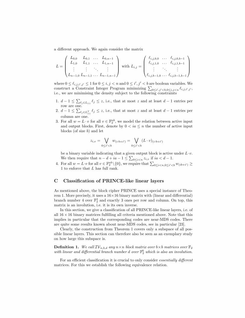
C Classification of PRINCE-like linear layers

As mentioned above, the block cipher PRINCE uses a special instance of Theo-rem 1. More precisely, it uses a 16×16 binary matrix with (linear and differential)branch number 4 over F4

2 and exactly 3 ones per row and column. On top, thismatrix is an involution, i.e. it is its own inverse.

In this section, we give a classification of all PRINCE-like linear layers, i.e. ofall 16× 16 binary matrices fulfilling all criteria mentioned above. Note that thisimplies in particular that the corresponding codes are near-MDS codes. Thereare quite some results known about near-MDS codes, see in particular [23].

Clearly, the construction from Theorem 1 covers only a subspace of all pos-sible linear layers. This section can therefore also be seen as an exemplary studyon how large this subspace is.

Definition 1. We call IVn,b,d any n×n block matrix over b×b matrices over F2

with linear and differential branch number d over Fb2 which is also an involution.

For an efficient classification it is crucial to only consider essentially differentmatrices. For this we establish the following equivalence relation.

Lemma 3. Let A be IVn,b,d. Then,

B = P ·Q ·A ·QT · PT

is also IVn,b,d for P being a block permutation matrix – permuting b× b blocksas units – and Q being a block diagonal matrix of n× n permutation matrices.

Definition 2. We call two IVn,m,d matrices A and B equivalent if B = P ·Q ·A ·QT · PT for P,Q as in Lemma 3.

Finally, we need to pick a representative for each family. For this the definitionof a normal forms is helpful.

Definition 3. We call a matrix in IVn,b,k normal form< under < iff A

1. is IVn,b,k, and

2. is the smallest matrix under < satisfying these conditions.

There are many choices for the ordering < used in this definition. For imple-mentation reasons we picked an ordering which essentially is the natural orderingon an 256-bit integer representation of the binary matrices.

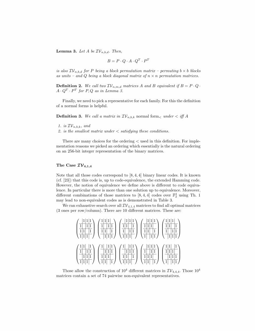
The Case IV4,1,4

Note that all those codes correspond to [8, 4, 4] binary linear codes. It is known(cf. [23]) that this code is, up to code-equivalence, the extended Hamming code.However, the notion of equivalence we define above is different to code equiva-lence. In particular there is more than one solution up to equivalence. Moreover,different combinations of those matrices to [8, 4, 4] codes over F4

2 using Th. 1may lead to non-equivalent codes as is demonstrated in Table 3.

We ran exhaustive search over all IV4,1,4 matrices to find all optimal matrices(3 ones per row/column). There are 10 different matrices. These are:

1 1 11 1 11 1 11 1 1

1 1 11 1 11 1 1

1 1 1

1 1 11 1 11 1 11 1 1

1 1 11 1 11 1 11 1 1

1 1 11 1 11 1 1

1 1 1

1 1 11 1 1

1 1 11 1 1

1 1 11 1 1

1 1 11 1 1

1 1 11 1 1

1 1 11 1 1

1 1 11 1 11 1 11 1 1

1 1 11 1 1

1 1 11 1 1

Those allow the construction of 104 different matrices in IV4,4,4. Those 104

matrices contain a set of 74 pairwise non-equivalent representatives.

The Case IV4,2,4

We then ran exhaustive search over all IV4,2,4 to find all optimal matrices (3ones per row/column). There are 220 different matrices satisfying the conditions.

Again, those matrices allow the construction of 2202 different matrices inIV4,4,4. The above mentioned equivalence relation reduced those to 470 essen-tially different matrices in IV4,4,4.

The Case IV4,4,4

Finally, we then ran exhaustive search on 16 × 16 matrices pruning any searchtree not satisfying the conditions of Lemma 1. Moreover, taking the equivalencerelation into account allows further pruning of search trees, resulting in a signif-icant speed up. In total, the whole search took less than one day on a standardPC.

There are 739 IV4,4,4 normal forms. Of those, 74 are composed of IV4,1,4

matrices and 470 are composed of IV4,2,4 matrices. The remaining 196 matricesare either not composed of IV4,i,4 matrices for i < 4 or are composed of IV4,3,4

and IV4,1,4 matrices.

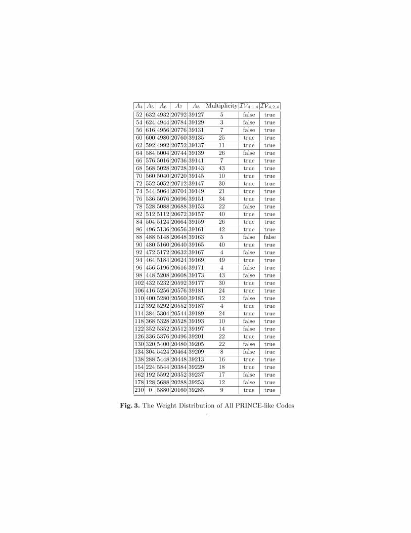
The Weight Distribution of IV4,4,4

One of the benefits of our classification is that the a-priori huge number of choicesfor a PRINCE-like linear layer is reduced to a much more manageable amount.This in particular allows to not only focus on the linear and differential branchnumber, but more detailed one the exact weight distribution of the correspondingadditive codes. While this does not improve the (directly) provable bounds onthe probabilities of linear and differential trails it has an impact on the numberof trails with optimal bias resp. probability. Note that, as proven in [23], theweight distribution of the code and its dual are identical. Moreover, given thenumber of code-words with minimal weight, the whole weight distribution isfixed (cf. [23, Theorem 4.1]).

Below we give an exhaustive list of the possible weight distributions for all739 PRINCE-like linear layers. Ai denotes the number of words with weight i. Wealso give the multiplicity, i.e. how many of the 739 cases lead to the given weightdistribution. We furthermore note which of the possible weight distributionsoccur for linear layers constructed via Theorem 1 either by combining IV4,1,4 orIV4,2,4 matrices. As can be seen, there is a rather big variance in the number ofcode words with minimal weight, ranging from 52 up to 210. While intuitively itseems beneficial to select a code with a minimal number of code words of smallweight, the exact benefits of a specific choice depend on cipher details outsidethe scope of this paper.

D Security Analysis of PRIDE

Due to following the interleaving construction it is straightforward to bound theprobability of differential characteristics and the absolute bias of linear trails.

A4 A5 A6 A7 A8 Multiplicity IV4,1,4 IV4,2,4

52 632 4932 20792 39127 5 false true

54 624 4944 20784 39129 3 false true

56 616 4956 20776 39131 7 false true

60 600 4980 20760 39135 25 true true

62 592 4992 20752 39137 11 true true

64 584 5004 20744 39139 26 false true

66 576 5016 20736 39141 7 true true

68 568 5028 20728 39143 43 true true

70 560 5040 20720 39145 10 true true

72 552 5052 20712 39147 30 true true

74 544 5064 20704 39149 21 true true

76 536 5076 20696 39151 34 true true

78 528 5088 20688 39153 22 false true

82 512 5112 20672 39157 40 true true

84 504 5124 20664 39159 26 true true

86 496 5136 20656 39161 42 true true

88 488 5148 20648 39163 5 false false

90 480 5160 20640 39165 40 true true

92 472 5172 20632 39167 4 false true

94 464 5184 20624 39169 49 true true

96 456 5196 20616 39171 4 false true

98 448 5208 20608 39173 43 false true

102 432 5232 20592 39177 30 true true

106 416 5256 20576 39181 24 true true

110 400 5280 20560 39185 12 false true

112 392 5292 20552 39187 4 true true

114 384 5304 20544 39189 24 true true

118 368 5328 20528 39193 10 false true

122 352 5352 20512 39197 14 false true

126 336 5376 20496 39201 22 true true

130 320 5400 20480 39205 22 false true

134 304 5424 20464 39209 8 false true

138 288 5448 20448 39213 16 true true

154 224 5544 20384 39229 18 true true

162 192 5592 20352 39237 17 false true

178 128 5688 20288 39253 12 false true

210 0 5880 20160 39285 9 true true

Fig. 3. The Weight Distribution of All PRINCE-like Codes.

We also investigated in detail if there is a significant linear-hull or differentialeffect.

Here, we justify our assumption of the resistance of PRIDE against classicalanalysis techniques, such as linear and differential cryptanalysis.

Classical Cryptanalysis. As mentioned above the differential and linear branchnumbers of L0 to L3 are all 4. Thus, it follows by Theorem 1 that the same holdsfor the entire linear layer L. This means we have –at least– 4 active Sboxes pertwo rounds and thus 32 in 16 rounds. For the Sboxes we selected, the best non-zero differential has probability 1/4. Thus, assuming independent round keys,there is no single differential trail for 16 rounds of PRIDE with average proba-bility better than (1/4)

32= 2−64, which is too small to be usable for an attack

even when using the full code-book. Similarly, for linear cryptanalysis, we canupper-bound the absolute correlation for any single trail by (1/2)

32= 2−32.

Again, this is too small to be of use in an attack.

We have computationally generated all optimal characteristics and trails forsix rounds of PRIDE. We found 15 871 differentials with probability 2−24 and5 632 trails with the expected absolute correlation of 2−12. Each optimal char-acteristic (resp. trail) has a unique pair of input and output difference (resp.mask). In other words, there is no clustering of neither optimal characteristicsnor optimal trails.

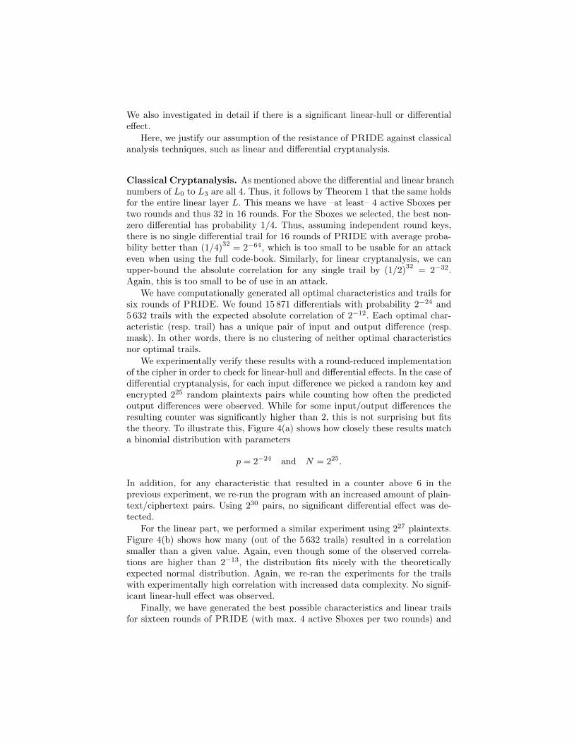
We experimentally verify these results with a round-reduced implementationof the cipher in order to check for linear-hull and differential effects. In the case ofdifferential cryptanalysis, for each input difference we picked a random key andencrypted 225 random plaintexts pairs while counting how often the predictedoutput differences were observed. While for some input/output differences theresulting counter was significantly higher than 2, this is not surprising but fitsthe theory. To illustrate this, Figure 4(a) shows how closely these results matcha binomial distribution with parameters

p = 2−24 and N = 225.

In addition, for any characteristic that resulted in a counter above 6 in theprevious experiment, we re-run the program with an increased amount of plain-text/ciphertext pairs. Using 230 pairs, no significant differential effect was de-tected.

For the linear part, we performed a similar experiment using 227 plaintexts.Figure 4(b) shows how many (out of the 5 632 trails) resulted in a correlationsmaller than a given value. Again, even though some of the observed correla-tions are higher than 2−13, the distribution fits nicely with the theoreticallyexpected normal distribution. Again, we re-ran the experiments for the trailswith experimentally high correlation with increased data complexity. No signif-icant linear-hull effect was observed.

Finally, we have generated the best possible characteristics and linear trailsfor sixteen rounds of PRIDE (with max. 4 active Sboxes per two rounds) and

0 2 4 6 8 100

500

1000

1500

2000

2500

3000

3500

4000

# of occurences

# o

f ch

ara

cte

ristics

binomial distribution

experiment

(a) Occurences of differential characteris-tics

0 −15−14 −13 −12 −110

1000

2000

3000

4000

5000

log2(correlation)

# o

f tr

ails

normal distribution

experiment

(b) Correlation of linear trails

Fig. 4. Experimental results for differential and linear cryptanalysis over sixrounds of PRIDE

found that there is no clustering of those optimal trails/characteristics. Ad-ditionally, our program shows that the bounds we have established are tight.However, PRIDE has 20 rounds; and in our belief, it should be sufficient.

Other Attacks. We also considered advanced variants of linear and differen-tial attacks. Higher-order differentials, truncated differentials, impossible differ-entials, and zero-correlation attacks do not seem to pose a threat on PRIDE.It seems that the bit-wise structure of the linear-layer limit the applicability ofthese attacks.

Finally, we have considered algebraic attacks, but did not find any seriousissues.

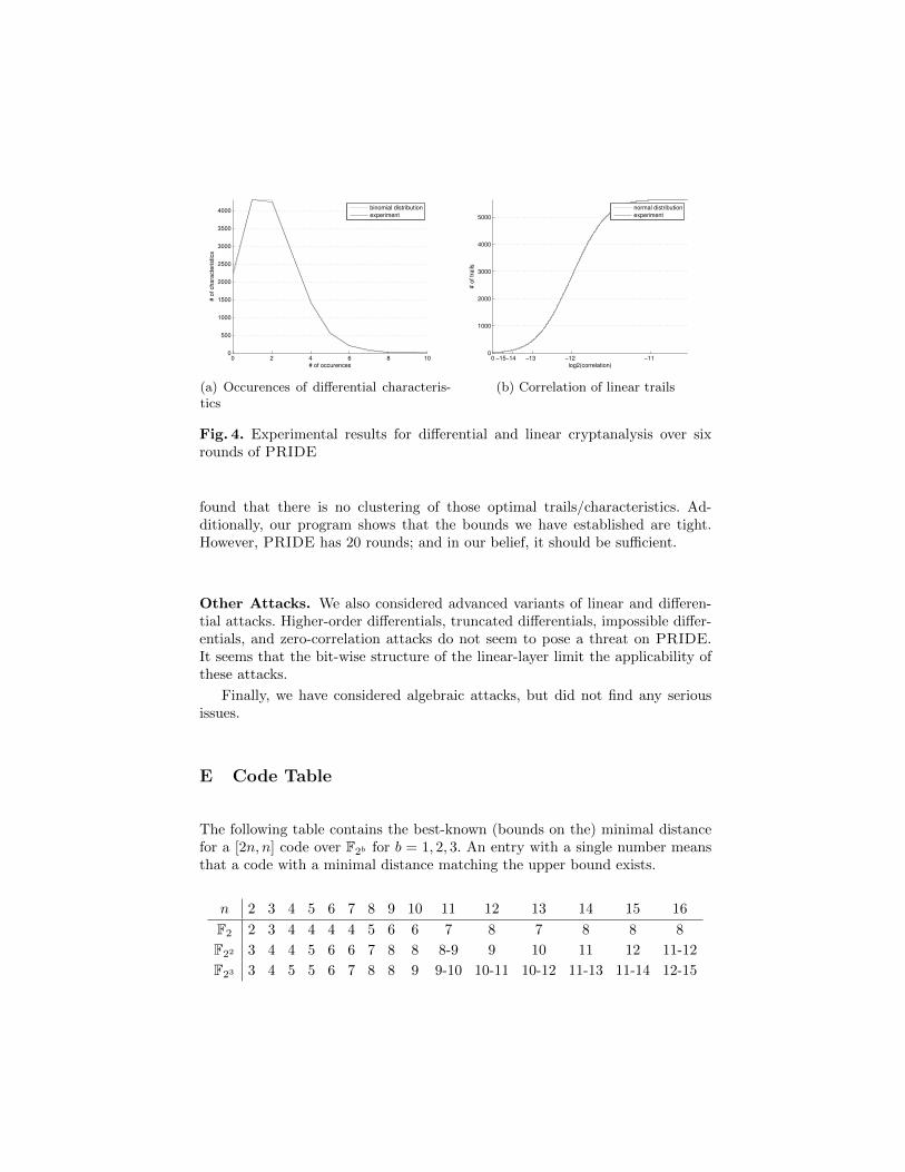
E Code Table

The following table contains the best-known (bounds on the) minimal distancefor a [2n, n] code over F2b for b = 1, 2, 3. An entry with a single number meansthat a code with a minimal distance matching the upper bound exists.

n 2 3 4 5 6 7 8 9 10 11 12 13 14 15 16

F2 2 3 4 4 4 4 5 6 6 7 8 7 8 8 8

F22 3 4 4 5 6 6 7 8 8 8-9 9 10 11 12 11-12

F23 3 4 5 5 6 7 8 8 9 9-10 10-11 10-12 11-13 11-14 12-15

F Algorithms for Finding Permutations MaximizingDependencies

F.1 Heuristic

We represent the permutations P,Q as integer vectors (p0, . . . , pn−1) with i′ ≤pi′ < n. This format is also known as LAPACK-style permutations and allowsto apply permutations to matrices in place. This format is interpreted by loop-ing over 0 ≤ i′ < n in increasing order and swapping row/column at index i′

with row/column at index pi′ . Our first algorithm simply finds local optima andcombines them. It fixes P0, Q0 to the identity (without loss of generality) anditerates over 1 ≤ i < b. For each level it proceeds index-wise. That is, for eachindex i′, it tries all possible values for p′i and q′i in Pi and Qi and keeps the valuewhich maximizes fill-in locally. It then proceeds to the next index.

F.2 Complete – Constraint Integer Program

We consider matrices

Pi =

pi,0,0 pi,0,1 . . . pi,0,n−1pi,1,0 pi,1,1 . . . pi,1,n−1

......

. . ....

pi,n−1,0 pi,n−1,1 . . . pi,n−1,n−1

, Qi =

qi,0,0 qi,0,1 . . . qi,0,n−1qi,1,0 qi,1,1 . . . qi,1,n−1

......

. . ....

qi,n−1,0 qi,n−1,1 . . . qi,n−1,n−1

.

and denote p`qi,0,0 p`qi,0,1 . . . p`qi,0,n−1p`qi,1,0 p`qi,1,1 . . . p`qi,1,n−1

......

. . ....

p`qi,n−1,0 p`qi,n−1,1 . . . p`qi,n−1,n−1

= Pi · L0 ·Qi.

1. We add quadratic constraints expressing p`qi′,i,j in terms of Pi′ · L0 ·Qi′ .

2. We add linear constraints expressing that all rows and columns of Pi′ andQi′ have exactly one 1 per row/column.

3. We add OR constraints vi,j =(∨

0≤i′<b paqi′,i,j

).

4. We add a linear constraint 1 ≤∑

vi,j ≤ b · (∑

0≤i,j<n ci) to encode that weonly have a limited number of ones to use for fill-in.

We then maximize∑

vi,j using an off-the-shelf CIP solver such as SCIP [1].

F.3 Example

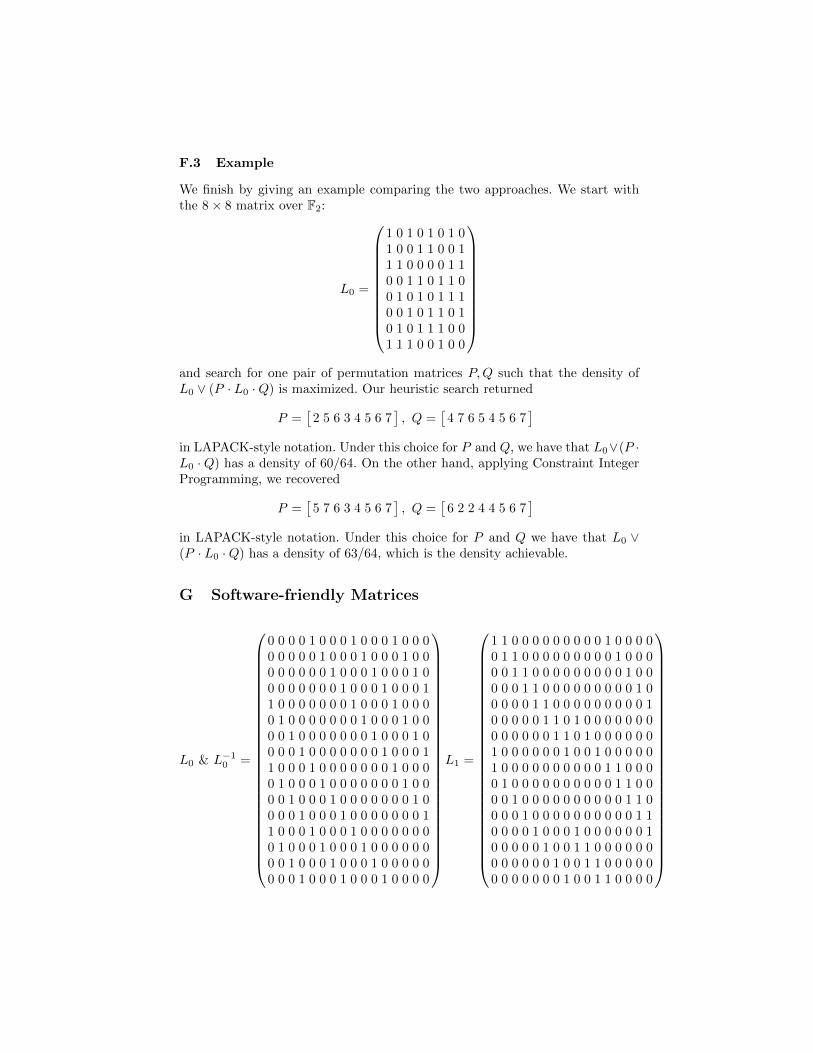
We finish by giving an example comparing the two approaches. We start withthe 8× 8 matrix over F2:

L0 =

1 0 1 0 1 0 1 01 0 0 1 1 0 0 11 1 0 0 0 0 1 10 0 1 1 0 1 1 00 1 0 1 0 1 1 10 0 1 0 1 1 0 10 1 0 1 1 1 0 01 1 1 0 0 1 0 0

and search for one pair of permutation matrices P,Q such that the density ofL0 ∨ (P · L0 ·Q) is maximized. Our heuristic search returned

P =[

2 5 6 3 4 5 6 7], Q =

[4 7 6 5 4 5 6 7

]in LAPACK-style notation. Under this choice for P and Q, we have that L0∨(P ·L0 ·Q) has a density of 60/64. On the other hand, applying Constraint IntegerProgramming, we recovered

P =[

5 7 6 3 4 5 6 7], Q =

[6 2 2 4 4 5 6 7

]in LAPACK-style notation. Under this choice for P and Q we have that L0 ∨(P · L0 ·Q) has a density of 63/64, which is the density achievable.

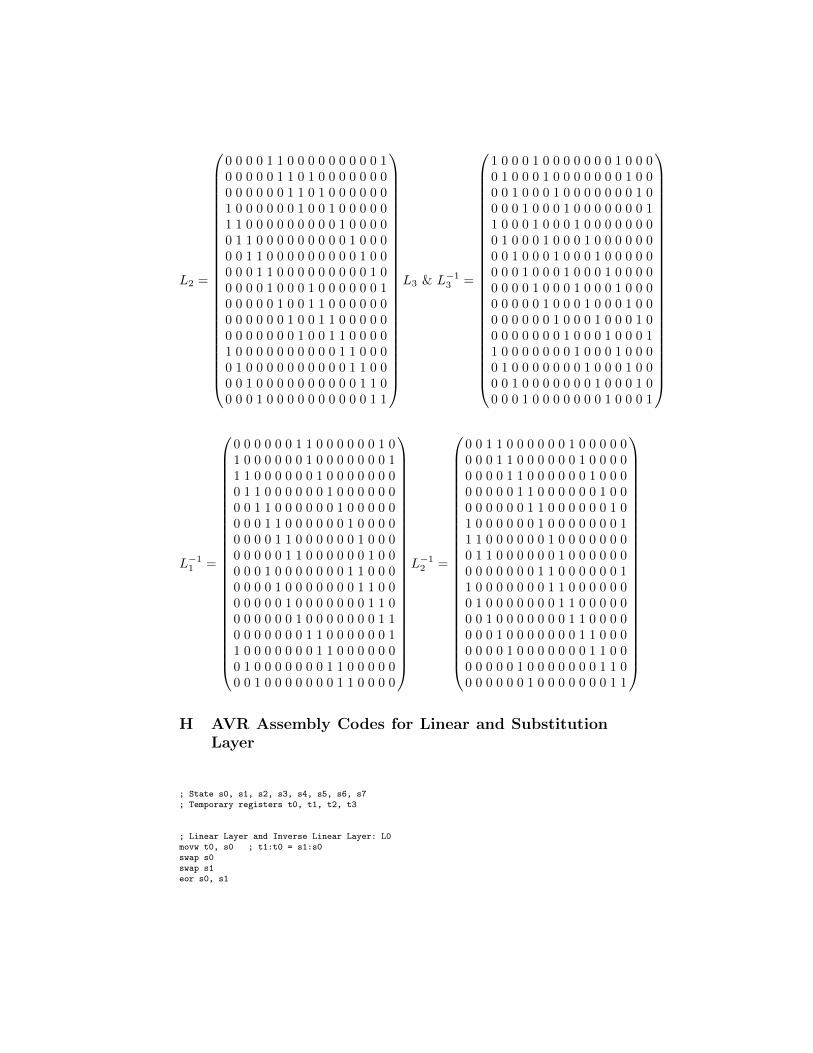
G Software-friendly Matrices

L0 & L−10 =

0 0 0 0 1 0 0 0 1 0 0 0 1 0 0 00 0 0 0 0 1 0 0 0 1 0 0 0 1 0 00 0 0 0 0 0 1 0 0 0 1 0 0 0 1 00 0 0 0 0 0 0 1 0 0 0 1 0 0 0 11 0 0 0 0 0 0 0 1 0 0 0 1 0 0 00 1 0 0 0 0 0 0 0 1 0 0 0 1 0 00 0 1 0 0 0 0 0 0 0 1 0 0 0 1 00 0 0 1 0 0 0 0 0 0 0 1 0 0 0 11 0 0 0 1 0 0 0 0 0 0 0 1 0 0 00 1 0 0 0 1 0 0 0 0 0 0 0 1 0 00 0 1 0 0 0 1 0 0 0 0 0 0 0 1 00 0 0 1 0 0 0 1 0 0 0 0 0 0 0 11 0 0 0 1 0 0 0 1 0 0 0 0 0 0 00 1 0 0 0 1 0 0 0 1 0 0 0 0 0 00 0 1 0 0 0 1 0 0 0 1 0 0 0 0 00 0 0 1 0 0 0 1 0 0 0 1 0 0 0 0

L1 =

1 1 0 0 0 0 0 0 0 0 0 1 0 0 0 00 1 1 0 0 0 0 0 0 0 0 0 1 0 0 00 0 1 1 0 0 0 0 0 0 0 0 0 1 0 00 0 0 1 1 0 0 0 0 0 0 0 0 0 1 00 0 0 0 1 1 0 0 0 0 0 0 0 0 0 10 0 0 0 0 1 1 0 1 0 0 0 0 0 0 00 0 0 0 0 0 1 1 0 1 0 0 0 0 0 01 0 0 0 0 0 0 1 0 0 1 0 0 0 0 01 0 0 0 0 0 0 0 0 0 0 1 1 0 0 00 1 0 0 0 0 0 0 0 0 0 0 1 1 0 00 0 1 0 0 0 0 0 0 0 0 0 0 1 1 00 0 0 1 0 0 0 0 0 0 0 0 0 0 1 10 0 0 0 1 0 0 0 1 0 0 0 0 0 0 10 0 0 0 0 1 0 0 1 1 0 0 0 0 0 00 0 0 0 0 0 1 0 0 1 1 0 0 0 0 00 0 0 0 0 0 0 1 0 0 1 1 0 0 0 0

L2 =

0 0 0 0 1 1 0 0 0 0 0 0 0 0 0 10 0 0 0 0 1 1 0 1 0 0 0 0 0 0 00 0 0 0 0 0 1 1 0 1 0 0 0 0 0 01 0 0 0 0 0 0 1 0 0 1 0 0 0 0 01 1 0 0 0 0 0 0 0 0 0 1 0 0 0 00 1 1 0 0 0 0 0 0 0 0 0 1 0 0 00 0 1 1 0 0 0 0 0 0 0 0 0 1 0 00 0 0 1 1 0 0 0 0 0 0 0 0 0 1 00 0 0 0 1 0 0 0 1 0 0 0 0 0 0 10 0 0 0 0 1 0 0 1 1 0 0 0 0 0 00 0 0 0 0 0 1 0 0 1 1 0 0 0 0 00 0 0 0 0 0 0 1 0 0 1 1 0 0 0 01 0 0 0 0 0 0 0 0 0 0 1 1 0 0 00 1 0 0 0 0 0 0 0 0 0 0 1 1 0 00 0 1 0 0 0 0 0 0 0 0 0 0 1 1 00 0 0 1 0 0 0 0 0 0 0 0 0 0 1 1

L3 & L−13 =

1 0 0 0 1 0 0 0 0 0 0 0 1 0 0 00 1 0 0 0 1 0 0 0 0 0 0 0 1 0 00 0 1 0 0 0 1 0 0 0 0 0 0 0 1 00 0 0 1 0 0 0 1 0 0 0 0 0 0 0 11 0 0 0 1 0 0 0 1 0 0 0 0 0 0 00 1 0 0 0 1 0 0 0 1 0 0 0 0 0 00 0 1 0 0 0 1 0 0 0 1 0 0 0 0 00 0 0 1 0 0 0 1 0 0 0 1 0 0 0 00 0 0 0 1 0 0 0 1 0 0 0 1 0 0 00 0 0 0 0 1 0 0 0 1 0 0 0 1 0 00 0 0 0 0 0 1 0 0 0 1 0 0 0 1 00 0 0 0 0 0 0 1 0 0 0 1 0 0 0 11 0 0 0 0 0 0 0 1 0 0 0 1 0 0 00 1 0 0 0 0 0 0 0 1 0 0 0 1 0 00 0 1 0 0 0 0 0 0 0 1 0 0 0 1 00 0 0 1 0 0 0 0 0 0 0 1 0 0 0 1

L−11 =

0 0 0 0 0 0 1 1 0 0 0 0 0 0 1 01 0 0 0 0 0 0 1 0 0 0 0 0 0 0 11 1 0 0 0 0 0 0 1 0 0 0 0 0 0 00 1 1 0 0 0 0 0 0 1 0 0 0 0 0 00 0 1 1 0 0 0 0 0 0 1 0 0 0 0 00 0 0 1 1 0 0 0 0 0 0 1 0 0 0 00 0 0 0 1 1 0 0 0 0 0 0 1 0 0 00 0 0 0 0 1 1 0 0 0 0 0 0 1 0 00 0 0 1 0 0 0 0 0 0 0 1 1 0 0 00 0 0 0 1 0 0 0 0 0 0 0 1 1 0 00 0 0 0 0 1 0 0 0 0 0 0 0 1 1 00 0 0 0 0 0 1 0 0 0 0 0 0 0 1 10 0 0 0 0 0 0 1 1 0 0 0 0 0 0 11 0 0 0 0 0 0 0 1 1 0 0 0 0 0 00 1 0 0 0 0 0 0 0 1 1 0 0 0 0 00 0 1 0 0 0 0 0 0 0 1 1 0 0 0 0

L−12 =

0 0 1 1 0 0 0 0 0 0 1 0 0 0 0 00 0 0 1 1 0 0 0 0 0 0 1 0 0 0 00 0 0 0 1 1 0 0 0 0 0 0 1 0 0 00 0 0 0 0 1 1 0 0 0 0 0 0 1 0 00 0 0 0 0 0 1 1 0 0 0 0 0 0 1 01 0 0 0 0 0 0 1 0 0 0 0 0 0 0 11 1 0 0 0 0 0 0 1 0 0 0 0 0 0 00 1 1 0 0 0 0 0 0 1 0 0 0 0 0 00 0 0 0 0 0 0 1 1 0 0 0 0 0 0 11 0 0 0 0 0 0 0 1 1 0 0 0 0 0 00 1 0 0 0 0 0 0 0 1 1 0 0 0 0 00 0 1 0 0 0 0 0 0 0 1 1 0 0 0 00 0 0 1 0 0 0 0 0 0 0 1 1 0 0 00 0 0 0 1 0 0 0 0 0 0 0 1 1 0 00 0 0 0 0 1 0 0 0 0 0 0 0 1 1 00 0 0 0 0 0 1 0 0 0 0 0 0 0 1 1

H AVR Assembly Codes for Linear and Substitution

Layer

; State s0, s1, s2, s3, s4, s5, s6, s7; Temporary registers t0, t1, t2, t3

; Linear Layer and Inverse Linear Layer: L0movw t0, s0 ; t1:t0 = s1:s0swap s0swap s1eor s0, s1

eor t0, s0mov s1, t0eor s0, t1

; Linear Layer: L1swap s3movw t0, s2 ; t1:t0 = s3:s2movw t2, s2 ; t3:t2 = s3:s2lsl t0rol t2lsr t1ror t3eor s2, t3mov t0, s2eor s2, t2eor s3, t0

; Inverse Linear Layer: L1movw t0, s2 ; t1:t0 = s3:s2movw t2, s2 ; t3:t2 = s3:s2lsr t0ror t2lsr t1ror t3eor t3, t2eor s3, t3swap s3mov s2, t3lsr t3ror s2eor s2, t2

; Linear Layer: L2swap s4movw t0, s4 ; t1:t0 = s5:s4movw t2, s4 ; t3:t2 = s5:s4lsl t0rol t2lsr t1ror t3eor s4, t3mov t0, s4eor s4, t2eor s5, t0

; Inverse Linear Layer: L2movw t0, s4 ; t1:t0 = s5:s4movw t2, s4 ; t3:t2 = s5:s4lsr t0ror t2lsr t1ror t3eor t3, t2eor s5, t3mov s4, t3lsr t3ror s4eor s4, t2swap s4

; Linear Layer and Inverse Linear Layer: L3movw t0, s6 ; t1:t0 = s7:s6swap s6swap s7eor s6, s7eor t1, s6mov s7, t1eor s6, t0

; Substitution Layermovw t0, s0movw t2, s2and s0, s2eor s0, s4and s2, s4eor s2, s6and s1, s3eor s1, s5and s3, s5eor s3, s7movw s4, s0movw s6, s2and s4, s6eor s4, t0and s6, s4eor s6, t2and s5, s7eor s5, t1and s7, s5eor s7, t3

I Sbox Formulation

A = c⊕ (a&b)

B = d⊕ (b&c)

C = a⊕ (A&B)

D = b⊕ (B&C)

J Testvectors for PRIDE

Plaintext k0 k1 Ciphertext

0000000000000000 0000000000000000 0000000000000000 82b4109fcc70bd1f

ffffffffffffffff 0000000000000000 0000000000000000 d70e60680a17b956

0000000000000000 ffffffffffffffff 0000000000000000 28f19f97f5e846a9

0000000000000000 0000000000000000 ffffffffffffffff d123ebaf368fce62

0123456789abcdef 0000000000000000 fedcba9876543210 d1372929712d336e

block ciphers { focus on the linear layer (feat. · block ciphers { focus on the linear layer...

Documents