blindsourceseparationbasedonjoint … · journal of statistical software 3 2....

JSS Journal of Statistical SoftwareJanuary 2017 Volume 76 Issue 2 doi 1018637jssv076i02

Blind Source Separation Based on JointDiagonalization in R The Packages JADE

and BSSasymp

Jari MiettinenUniversity of Jyvaskyla

Klaus NordhausenUniversity of Turku

Sara TaskinenUniversity of Jyvaskyla

Abstract

Blind source separation (BSS) is a well-known signal processing tool which is used tosolve practical data analysis problems in various fields of science In BSS we assume thatthe observed data consists of linear mixtures of latent variables The mixing system andthe distributions of the latent variables are unknown The aim is to find an estimate of anunmixing matrix which then transforms the observed data back to latent sources In thispaper we present the R packages JADE and BSSasymp The package JADE offers severalBSS methods which are based on joint diagonalization Package BSSasymp containsfunctions for computing the asymptotic covariance matrices as well as their data-basedestimates for most of the BSS estimators included in package JADE Several simulatedand real datasets are used to illustrate the functions in these two packages

Keywords independent component analysis multivariate time series nonstationary sourceseparation performance indices second order source separation

1 IntroductionThe blind source separation (BSS) problem is in its most simple form the following Assumethat observations x1 xn are p-variate vectors whose components are linear combinationsof the components of p-variate unobservable zero mean vectors z1 zn If we consider p-variate vectors x and z as row vectors (to be consistent with the programming language R RCore Team 2016) the BSS model can be written as

x = zAgt + micro (1)

where A is an unknown full rank p times p mixing matrix and micro is a p-variate location vectorThe goal is then to estimate an unmixing matrix W = Aminus1 based on the ntimes p data matrix

2 JADE and BSSasymp Blind Source Separation in R

X = [xgt1 xgtn ]gt such that zi = (xi minus micro)Wgt i = 1 n Notice that BSS can also beapplied in cases where the dimension of x is larger than that of z by applying a dimensionreduction method as a first stage In this paper we however restrict to the case where A isa square matrixThe unmixing matrix W cannot be estimated without further assumptions on the modelThere are three major BSS models which differ in their assumptions made upon z In inde-pendent component analysis (ICA) which is the most popular BSS approach it is assumedthat the components of z are mutually independent and at most one of them is GaussianICA applies best to cases where also z1 zn are independent and identically distributed(iid) The two other main BSS models the second order source separation (SOS) modeland the second order nonstationary source separation (NSS) model utilize temporal or spa-tial dependence within each component In the SOS model the components are assumed tobe uncorrelated weakly (second-order) stationary time series with different time dependencestructures The NSS model differs from the SOS model in that the variances of the time seriescomponents are allowed to be nonstationary All these three models will be defined in detaillater in this paperNone of the three models has a unique solution This can be seen by choosing any p times pmatrix C from the set

C = C each row and column of C has exactly one non-zero element (2)

Then C is invertible Alowast = ACminus1 is of full rank the components of zlowast = zCgt are uncorrelated(and independent in ICA) and the model can be rewritten as x = zlowastAlowast

gt Thus the ordersigns and scales of the source components cannot be determined This means that for anygiven unmixing matrix W also W lowast = CW with C isin C is a solutionAs the scales of the latent components are not identifiable one may simply assume thatCOV(z) = Ip Let then Σ = COV(x) = AAgt denote the covariance matrix of x and furtherlet Σminus12 be the symmetric matrix satisfying Σminus12Σminus12 = Σminus1 Then for the standardizedrandom variable xst = (xminus micro)Σminus12 we have that z = xstU

gt for some orthogonal U (Mietti-nen Taskinen Nordhausen and Oja 2015b Theorem 1) Thus the search for the unmixingmatrix W can be separated into finding the whitening (standardization) matrix Σminus12 andthe rotation matrix U The unmixing matrix is then given by W = UΣminus12In this paper we describe the R package JADE (Nordhausen Cardoso Miettinen Oja Ollilaand Taskinen 2017) which offers several BSS methods covering all three major BSS modelsIn all of these methods the whitening step is performed using the regular covariance matrixwhereas the rotation matrix U is found via joint diagonalization The concepts of simul-taneous and approximate joint diagonalization are recalled in Section 2 and several ICASOS and NSS methods based on diagonalization are described in Sections 3 4 and 5 respec-tively As performance indices are widely used to compare different BSS algorithms we definesome popular indices in Section 6 We also introduce the R package BSSasymp (MiettinenNordhausen Oja and Taskinen 2017) which includes functions for computing the asymptoticcovariance matrices and their data-based estimates for most of the BSS estimators in thepackage JADE Section 7 describes the R packages JADE and BSSasymp and in Section 8we illustrate the use of these packages via simulated and real data examples

Journal of Statistical Software 3

2 Simultaneous and approximate joint diagonalization

21 Simultaneous diagonalization of two symmetric matrices

Let S1 and S2 be two symmetric p times p matrices If S1 is positive definite then there is anonsingular ptimes p matrix W and a diagonal ptimes p matrix D such that

WS1Wgt = Ip and WS2W

gt = D

If the diagonal values of D are distinct the matrix W is unique up to a permutation andsign changes of the rows Notice that the requirement that either S1 or S2 is positive definiteis not necessary there are more general results on simultaneous diagonalization of two sym-metric matrices see for example Golub and Van Loan (2002) However for our purposes theassumption of positive definiteness is not too strongThe simultaneous diagonalizer can be solved as follows First solve the eigenvalueeigenvectorproblem

S1Vgt = V gtΛ1

and define the inverse of the square root of S1 as

Sminus121 = V gtΛminus12

1 V

Next solve the eigenvalueeigenvector problem

(Sminus121 S2(Sminus12

1 )gt)Ugt = UgtΛ2

The simultaneous diagonalizer is then W = USminus121 and D = Λ2

22 Approximate joint diagonalization

Exact diagonalization of a set of symmetric ptimes p matrices S1 SK K gt 2 is only possibleif all matrices commute As shown later in Sections 3 4 and 5 in BSS this is however notthe case for finite data and we need to perform approximate joint diagonalization that iswe try to make WSKW

gt as diagonal as possible In practice we have to choose a measureof diagonality M a function that maps a set of p times p matrices to [0infin) and seek W thatminimizes

Ksumk=1

M(WSkWgt)

Usually the measure of diagonality is chosen to be

M(V ) = off(V )2 =sumi 6=j

(V )2ij

where off(V ) has the same off-diagonal elements as V and the diagonal elements are zeroIn common principal component analysis for positive definite matrices Flury (1984) used themeasure

M(V ) = log det(diag(V ))minus log det(V )

where diag(V ) = V minus off(V )


Obviously the sum of squares criterion is minimized by the trivial solution W = 0 The mostpopular method to avoid this solution is to diagonalize one of the matrices then transformthe rest of the Kminus1 matrices and approximately diagonalize them requiring the diagonalizerto be orthogonal To be more specific suppose that S1 is a positive definite p times p matrixThen find S

minus121 and denote Slowastk = S

minus121 Sk(Sminus12

1 )gt k = 2 K Notice that in classicalBSS methods matrix S1 is usually the covariance matrix and the transformation is calledwhitening Now if we measure the diagonality using the sum of squares of the off-diagonalelements the approximate joint diagonalization problem is equivalent to finding an orthogonalptimes p matrix U that minimizes

Ksumk=2off(USlowastkUgt)2 =

Ksumk=2

sumi 6=j

(USlowastkUgt)2ij

Since the sum of squares remains the same when multiplied by an orthogonal matrix we mayequivalently maximize the sum of squares of the diagonal elements

Ksumk=2diag(USlowastkUgt)2 =

Ksumk=2

psumi=1

(USlowastkUgt)2ii (3)

Several algorithms for orthogonal approximate joint diagonalization have been suggestedand in the following we describe two algorithms which are given in the R package JADEFor examples of nonorthogonal approaches see R package jointDiag (Gouy-Pailler 2009) andreferences therein as well as Yeredor (2002)The rjd algorithm uses Givenrsquos (or Jacobi) rotations to transform the set of matrices toa more diagonal form two rows and two columns at a time (Clarkson 1988) The Givensrotation matrix is given by

G(i j θ) =

1 middot middot middot 0 middot middot middot 0 middot middot middot 0

0 middot middot middot cos(θ) middot middot middot minus sin(θ) middot middot middot 0

0 middot middot middot sin(θ) middot middot middot cos(θ) middot middot middot 0


In the rjd algorithm the initial value for the orthogonal matrix U is Ip First the valueof θ is computed using the elements (Slowastk)11 (Slowastk)12 and (Slowastk)22 k = 2 K and matricesU Slowast2 S

lowastK are then updated by

U larr UG(1 2 θ) and Slowastk larr G(1 2 θ)SlowastkG(1 2 θ) k = 2 K

Similarly all pairs i lt j are gone through When θ = 0 the Givens rotation matrix is theidentity and no more rotation is done Hence the convergence has been reached when θ issmall for all pairs i lt j Based on vast simulation studies it seems that the solution of therjd algorithm always maximizes the diagonality criterion (3)In the deflation based joint diagonalization (djd) algorithm the rows of the joint diagonalizerare found one by one (Nordhausen Gutch Oja and Theis 2012) Following the notations


above assume that Slowast2 SlowastK K ge 2 are the symmetric p times p matrices to be jointlydiagonalized by an orthogonal matrix and write the criterion (3) as


psumj=1

Ksumk=2

(ujSlowastkugtj )2 (4)

where uj is the jth row of U The sum (4) can then be approximately maximized by solvingsuccessively for each j = 1 pminus 1 uj that maximizes

Ksumk=2


under the constraint urugtj = δrj r = 1 j minus 1 Recall that δrj = 1 if r = j and zerootherwiseThe djd algorithm in the R package JADE is based on gradients and to avoid stopping atlocal maxima the initial value for each row is chosen from a set of random vectors so thatcriterion (5) is maximized in that set The djd function also has an option to choose the initialvalues to be the eigenvectors of the first matrix Slowast2 which makes the function faster but doesnot guarantee that the global maximum is reached Recall that even if the algorithm finds theglobal maximum in every step the solution only approximately maximizes the criterion (4)In the djd function also criteria of the form

Ksumk=2|ujSlowastkugtj |r r gt 0

can be used instead of (5) and if all matrices are positive definite also

Ksumk=2

log(ujSlowastkugtj )

The joint diagonalization plays an important role is BSS In the next sections we recall thethree major BSS models and corresponding separation methods which are based on the jointdiagonalization All these methods are included in the R package JADE

3 Independent component analysisThe independent component model assumes that the source vector z in model (1) has mutuallyindependent components Based on this assumption the mixing matrix A in (1) is not well-defined therefore some extra assumptions are usually made Common assumptions on thesource variable z in the IC model are

(IC1) the source components are mutually independent

(IC2) E(z) = 0 and E(zgtz) = Ip

(IC3) at most one of the components is Gaussian and


(IC4) each source component is independent and identically distributed

Assumption (IC2) fixes the variances of the components and thus the scales of the rowsof A Assumption (IC3) is needed as for multiple normal components independence anduncorrelatedness are equivalent Thus any orthogonal transformation of normal componentspreserves the independenceClassical ICA methods are often based on maximizing the non-Gaussianity of the componentsThis approach is motivated by the central limit theorem which roughly speaking says that thesum of random variables is more Gaussian than the summands Several different methods toperform ICA are proposed in the literature For general overviews see for example HyvaumlrinenKarhunen and Oja (2001) Comon and Jutten (2010) Oja and Nordhausen (2012) Yu Huand Xu (2014)In the following we review two classical ICA methods FOBI and JADE which utilize jointdiagonalization when estimating the unmixing matrix As the FOBI method is a special caseof ICA methods based on two scatter matrices with so-called independence property (OjaSirkiauml and Eriksson 2006) we will first recall some related definitions

31 Scatter matrix and independence propertyLet Fx denote the cumulative distribution function of a p-variate random vector x A matrixvalued functional S(Fx) is called a scatter matrix if it is positive definite symmetric andaffine equivariant in the sense that S(FAx+b) = AS(Fx)Agt for all x full rank ptimes p matricesA and all p-variate vectors bOja et al (2006) noticed that the simultaneous diagonalization of any two scatter matri-ces with the independence property yields the ICA solution The issue was further studiedin Nordhausen Oja and Ollila (2008a) A scatter matrix S(Fx) with the independence prop-erty is defined to be a diagonal matrix for all x with independent components An exampleof a scatter matrix with the independence property is the covariance matrix but when itcomes to most scatter matrices they do not possess the independence property (for moredetails see Nordhausen and Tyler 2015) However it was noticed in Oja et al (2006) that ifthe components of x are independent and symmetric then S(Fx) is diagonal for any scattermatrix Thus a symmetrized version of a scatter matrix Ssym(Fx) = S(Fx1minusx2) where x1 andx2 are independent copies of x always has the independence property and can be used tosolve the ICA problemThe affine equivariance of the matrices which are used in the simultaneous diagonalization andapproximate joint diagonalization methods implies the affine equivariance of the unmixingmatrix estimator More precisely if the unmixing matrices W and W lowast correspond to x andxlowast = xBgt respectively then xWgt = xlowastW lowast

gt (up to sign changes of the components) for allp times p full rank matrices B This is a desirable property of an unmixing matrix estimatoras it means that the separation result does not depend on the mixing procedure It is easyto see that the affine equivariance also holds even if S2 SK K ge 2 are only orthogonalequivariant

32 FOBIOne of the first ICA methods FOBI (fourth order blind identification) introduced by Cardoso(1989) uses simultaneous diagonalization of the covariance matrix and the matrix based on


the fourth moments

S1(Fx) = COV(x) and S2(Fx) = 1p+ 2E[Sminus12

1 (xminus E(x))2(xminus E(x))gt(xminus E(x))]

respectively Notice that both S1 and S2 are scatter matrices with the independence propertyThe unmixing matrix is the simultaneous diagonalizer W satisfying

WS1(Fx)Wgt = Ip and WS2(Fx)Wgt = D

where the diagonal elements of D are the eigenvalues of S2(Fz) given by E[z4i ] + p minus 1

i = 1 p Thus for a unique solution FOBI requires that the independent componentshave different kurtosis values The statistical properties of FOBI are studied in IlmonenNevalainen and Oja (2010a) and Miettinen et al (2015b)

33 JADE

The JADE (joint approximate diagonalization of eigenmatrices) algorithm (Cardoso andSouloumiac 1993) can be seen as a generalization of FOBI since both of them utilize fourthmoments For a recent comparison of these two methods see Miettinen et al (2015b) Con-trary to FOBI the kurtosis values do not have to be distinct in JADE The improvement isgained by increasing the number of matrices to be diagonalized as follows Define for anyptimes p matrix M the fourth order cumulant matrix as

C(M) = E[(xstMxgtst)xgtstxst ]minusM minusMgt minus tr(M)Ip

where xst is a standardized variable Notice that C(Ip) is the matrix based on the fourthmoments used in FOBI Write then Eij = egti ej i j = 1 p where ei is a p-vector with theith element one and others zero In JADE (after the whitening) the matrices C(Eij) i j =1 p are approximately jointly diagonalized by an orthogonal matrix The rotation matrixU thus maximizes the approximate joint diagonalization criterion

psumi=1

psumj=1diag(UC(Eij)Ugt)2

JADE is affine equivariant even though the matrices C(Eij) i j = 1 p are not orthog-onal equivariant If the eighth moments of the independent components are finite then thevectorized JADE unmixing matrix estimate has a limiting multivariate normal distributionFor the asymptotic covariance matrix and a detailed discussion about JADE see Miettinenet al (2015b)The JADE estimate jointly diagonalizes p2 matrices Hence its computational load growsquickly with the number of components Miettinen Nordhausen Oja and Taskinen (2013)suggested a quite similar but faster method called k-JADE which is computationally muchsimpler The k-JADE method whitens the data using FOBI and then jointly diagonalizes

C(Eij) i j = 1 p with |iminus j| lt k

The value k le p can be chosen by the user and corresponds basically to the guess of thelargest multiplicity of identical kurtosis values of the sources If k is larger or equal to thelargest multiplicity then k-JADE and JADE seem to be asymptotically equivalent


4 Second order source separationIn second order source separation (SOS) model the source vectors compose a p-variate timeseries z = (zt)t=0plusmn1plusmn2 that satisfies

(SOS1) E(zt) = 0 and E(zgtt zt) = Ip and

(SOS2) E(zgtt zt+τ ) = Dτ is diagonal for all τ = 1 2

Above assumptions imply that the components of z are weakly stationary and uncorrelatedtime series In the following we will shortly describe two classical (SOS) methods which yieldaffine equivariant unmixing matrix estimatesThe AMUSE (algorithm for multiple unknown signals extraction Tong Soon Huang andLiu 1990) uses the method of simultaneous diagonalization of two matrices In AMUSE thematrices to be diagonalized are the covariance matrix and the autocovariance matrix withchosen lag τ that is

S0(Fx) = COV(x) and Sτ (Fx) = E[(xt minus E(xt))gt(xt+τ minus E(xt))]

The unmixing matrix Wτ then satisfies

WτS0(Fx)Wgtτ = Ip and WτSτ (Fx)Wgtτ = Dτ

The requirement for distinct eigenvalues implies that the autocorrelations with the chosenlag need to be unequal for the source components Notice that as the population quantitySτ (Fx) is symmetric the estimate Wτ is obtained by diagonalizing the sample covariancematrix and the symmetrized autocovariance matrix with lag τ The sample autocovariancematrix with lag τ is given by

Sτ (X) = 1nminus τ

nminusτsumt=1

(Xt minus Xt)gt(Xt+τ minus Xt)

and the symmetrized autocovariance matrix with lag τ

SSτ (X) = 12(Sτ (X) + Sτ (X)gt)

respectivelyIt has been shown that the choice of the lag has a great impact on the performance of theAMUSE estimate (Miettinen Nordhausen Oja and Taskinen 2012) However without anypreliminary knowledge of the uncorrelated components it is difficult to choose the best lag forthe problem at hand Cichocki and Amari (2002) simply recommend to start with τ = 1 andcheck the diagonal elements of the estimate D If there are two almost equal values anothervalue for τ should be chosenBelouchrani Abed-Meraim Cardoso and Moulines (1997) provide a natural approximatejoint diagonalization method for the SOS model In SOBI (second order blind identifica-tion) the data is whitened using the covariance matrix S0(Fx) = COV(x) The K ma-trices for rotation are then autocovariance matrices with distinct lags τ1 τK that isSτ1(Fx) SτK (Fx) The use of different joint diagonalization methods yields estimates


with different properties For details about the deflation-based algorithm (djd) in SOBI seeMiettinen Nordhausen Oja and Taskinen (2014) and for details about SOBI using therjd algorithm see Miettinen Illner Nordhausen Oja Taskinen and Theis (2016) Generalagreement seems to be that in most cases the use of rjd in SOBI is preferableThe problem of choosing the set of lags τ1 τK for SOBI is not as important as thechoice of lag τ for AMUSE Among the signal processing community K = 12 and τk = kfor k = 1 K are conventional choices Miettinen et al (2014) argue that when thedeflation-based joint diagonalization is applied one should rather take too many matricesthan too few The same suggestion applies to SOBI using the rjd If the time series arelinear processes the asymptotic results in Miettinen et al (2016) provide tools to choose theset of lags see also Example 2 in Section 8

5 Nonstationary source separationThe SOS model assumptions are sometimes considered to be too strong The NSS model isa more general framework for cases where the data are ordered observations In addition tothe basic BSS model (1) assumptions the following assumptions on the source componentsare made

(NSS1) E(zt) = 0 for all t

(NSS2) E(zgtt zt) is positive definite and diagonal for all t

(NSS3) E(zgtt zt+τ ) is diagonal for all t and τ

Hence the source components are uncorrelated and they have a constant mean Howeverthe variances are allowed to change over time Notice that this definition differs from theblock-nonstationary model where the time series can be divided into intervals so that theSOS model holds for each intervalNSS-SD NSS-JD and NSS-TD-JD are algorithms that take into account the nonstationarityof the variances For the description of the algorithms define

STτ (Fx) = 1|T | minus τ

sumtisinT

E[(xt minus E(xt))gt(xt+τ minus E(xt))]

where T is a finite time interval and τ isin 0 1 The NSS-SD unmixing matrix simultaneously diagonalizes ST10(Fx) and ST20(Fx) whereT1 T2 sub [1 n] are separate time intervals T1 and T2 should be chosen so that ST10(Fx) andST20(Fx) are as different as possibleThe corresponding approximate joint diagonalization method is called NSS-JD The data iswhitened using the covariance matrix S[1n]0(Fx) computed from all the observations Af-ter whitening the K covariance matrices ST10(Fx) STK 0(Fx) related to time intervalsT1 TK are diagonalized with an orthogonal matrixBoth NSS-SD and NSS-JD algorithms ignore the possible time dependence Assume that thefull time series can be divided into K time intervals T1 TK so that in each interval theSOS model holds approximately Then the autocovariance matrices within the intervals makesense and the NSS-TD-JD algorithm is applicable Again the covariance matrix S[1n]0(Fx)


whitens the data Now the matrices to be jointly diagonalized are STiτj (Fx) i = 1 K j =1 L When selecting the intervals one should take into account the lengths of the intervalsso that the random effect is not too large when the covariances and the autocovariances arecomputed A basic rule among the signal processing community is to have 12 intervals ifthe data is large enough or K lt 12 intervals such that each interval contains at least 100observations Notice that NSS-SD and NSS-JD (as well as AMUSE and SOBI) are specialcases of NSS-TD-JD Naturally NSS-SD NSS-JD and NSS-TD-JD are all affine equivariantFor further details on NSS methods see for example Choi and Cichocki (2000ba) ChoiCichocki and Belouchrani (2001) Nordhausen (2014) Notice that asymptotic results are notyet available for any of these NSS methods

6 BSS performance criteriaThe performance of different BSS methods using real data is often difficult to evaluate sincethe true unmixing matrix is unknown In simulations studies however the situation is dif-ferent and in the literature many performance indices have been suggested to measure theperformance of different methods For a recent overview see Nordhausen Ollila and Oja(2011) for exampleThe package JADE contains several performance indices but in the following we will onlyintroduce two of them Both performance indices are functions of the so-called gain matrixG which is a product of the unmixing matrix estimate W and the true mixing matrix thatis G = WA Since the order the signs and the scales of the source components cannot beestimated the gain matrix of an optimal estimate does not have to be identity but equivalentto the identity in the sense that G = C for some C isin C where C is given in (2)The Amari error (Amari Cichocki and Yang 1996) is defined as

AE(G) = 12p(pminus 1)

psumi=1

psumj=1

|gij |maxh |gih|

minus 1

+psumj=1

( psumi=1

|gij |maxh |ghj |

minus 1)

where gij denotes the ijth element of G The range of the Amari error values is [0 1] anda small value corresponds to a good separation performance The Amari error is not scaleinvariant Therefore when different algorithms are compared the unmixing matrices shouldbe scaled in such a way that the corresponding rows of different matrices are of equal lengthThe minimum distance index (Ilmonen Nordhausen Oja and Ollila 2010b) is defined as

MD(G) = 1radicpminus 1 inf

CisinCCGminus Ip

where middot is the matrix (Frobenius) norm and C is defined in (2) Also the MD index isscaled to have a maximum value 1 and MD(G) = 0 if and only if G isin C The MD indexis affine invariant The statistical properties of the index are thoroughly studied in Ilmonenet al (2010b) and Ilmonen Nordhausen Oja and Ollila (2012)A feature that makes the minimum distance index especially attractive in simulation studiesis that its value can be related to the asymptotic covariance matrix of an estimator W IfW rarr Aminus1 and

radicn vec(WAminusIp)rarr Np2(0Σ) which is for example the case for FOBI JADE


AMUSE and SOBI then the limiting distribution of n(pminus 1)MD(G)2 has as expected value

tr((Ip2 minusDpp)Σ(Ip2 minusDpp)

) (6)

where Dpp = sumpi=1 e

gti ei otimes egti ei with otimes denoting the Kronecker product and ei a p-vector

with ith element one and others zeroNotice that tr

((Ip2 minusDpp)Σ(Ip2 minusDpp)

)is the sum of the off-diagonal elements of Σ and

therefore a natural measure of the variation of the unmixing matrix estimate W We willmake use of this relationship later in one of our examples

7 Functionality of the packagesThe package JADE is freely available from the Comprehensive R Archive Network (CRAN)at httpCRANR-projectorgpackage=JADE and comes under the GNU General PublicLicense (GPL) 20 or higherThe main functions of the package implement the blind source separation methods describedin the previous sections The function names are self explanatory being FOBI JADE andk_JADE for ICA AMUSE and SOBI for SOS and NSSSD NSSJD and NSSTDJD for NSS Allfunctions usually take as an input either a numerical matrix X or as alternative a multivariatetime series object of class lsquotsrsquo The functions have method appropriate arguments like forexample which lags to choose for AMUSE and SOBIAll functions return an object of the S3 class lsquobssrsquo which contains at least an object W whichis the estimated unmixing matrix and S containing the estimated (and centered) sourcesDepending on the chosen function also other information is stored The methods availablefor the class are

bull print which prints basically all information except the sources S

bull coef which extracts the unmixing matrix W

bull plot which produces a scatter plot matrix of S using pairs for ICA methods anda multivariate time series plot using the plot method for lsquotsrsquo objects for other BSSmethods

To extract the sources S the helper function bsscomponents can be usedThe functions which use joint approximate diagonalization of several matrices provide theuser an option to choose the method for joint diagonalization from the list below

bull djd for deflation-based joint diagonalization

bull rjd for joint diagonalization using Givens rotations

bull frjd which is basically the same as rjd but has less options and is much faster becauseit is implemented in C

From our experience the function frjd when appropriate seems to obtain the best results


In addition the JADE package provides two other functions for joint diagonalization Thefunction FG is designed for diagonalization of real positive-definite matrices and cjd is thegeneralization of rjd to the case of complex matrices For details about all functions for jointdiagonalization see also their help pages More functions for joint diagonalization are alsoavailable in the R package jointDiagTo evaluate the performance of BSS methods using simulation studies performance indicesare needed The package provides for this purpose the functions amari_error ComonGAP MDand SIR Our personal favorite is the MD function which implements the minimum distanceindex described in Section 6 For further details on all the functions see their help pages andthe references thereinFor ICA many alternative methods are implemented in other R packages Examples in-clude fastICA (Marchini Heaton and Ripley 2013) fICA (Miettinen Nordhausen Oja andTaskinen 2015a) mlica2 (Teschendorff 2012) PearsonICA (Karvanen 2009) and ProDenICA(Hastie and Tibshirani 2010) None of these ICA methods uses joint diagonalization in esti-mation Two slightly overlapping packages with JADE are ICS (Nordhausen Oja and Tyler2008b) which provides a generalization of the FOBI method and ica (Helwig 2015) whichincludes the JADE algorithm In current practice JADE and fastICA (implemented for exam-ple in the packages fastICA and fICA) seem to be the most often used ICA methods Othernewer ICA methods as for example ICA via product density estimation as provided in thepackage ProDenICA are often computationally very intensive as the sample size is usuallyhigh in typical ICA applications To the best of our knowledge there are currently no otherR packages for SOS or NSS availableMany methods included in the JADE package are also available in the MATLAB (The Math-Works Inc 2014) toolbox ICALAB (Cichocki Amari Siwek Tanaka Phan and others 2014)which accompanies the book of Cichocki and Amari (2002) A collection of links to JADE im-plementations for real and complex values in different languages like MATLAB C and Pythonas well as some joint diagonalization functions for MATLAB are available on J-F Cardosorsquoshomepage (httppersotelecom-paristechfr~cardosoguidesepsouhtml)The package BSSasymp is freely available from the Comprehensive R Archive Network (CRAN)at httpsCRANR-projectorgpackage=BSSasymp and comes under the GNU GeneralPublic License (GPL) 20 or higherThere are two kinds of functions in the package The first set of functions compute theasymptotic covariance matrices of the vectorized mixing and unmixing matrix estimates underdifferent BSS models The others estimate the covariance matrices based on a data matrixThe package BSSasymp includes functions for several estimators implemented in packageJADE These are FOBI and JADE in the IC model and AMUSE deflation-based SOBIand regular SOBI in the SOS model The asymptotic covariance matrices for FOBI andJADE estimates are computed using the results in Miettinen et al (2015b) For the limitingdistributions of AMUSE and SOBI estimates see Miettinen et al (2012) and Miettinen et al(2016) respectivelyFunctions ASCOV_FOBI and ASCOV_JADE compute the theoretical values for covariance matri-ces The argument sdf is the vector of source density functions standardized to have meanzero and variance equal to one supp is a two column matrix whose rows give the lowerand the upper limits used in numerical integration for each source component and A is themixing matrix The corresponding functions ASCOV_SOBIdefl and ASCOV_SOBI in the SOS


model take as input the matrix psi which gives the MA coefficients of the source time seriesthe vector of integers taus for the lags a matrix of fourth moments of the innovations Beta(default value is for Gaussian innovations) and the mixing matrix AFunctions ASCOV_FOBI_est ASCOV_JADE_est ASCOV_SOBIdefl_est and ASCOV_SOBI_estcan be used for approximating the covariance matrices of the estimates They are based onasymptotic results and therefore the sample size should not be very small Argument X canbe either the observed data or estimated source components When argument mixed is set toTRUE X is considered as observed data and the unmixing matrix is first estimated using themethod of interest The estimation of the covariance matrix of the SOBI estimate is also basedon the assumption that the time series are stationary linear processes If the time series areGaussian then the asymptotic variances and covariances depend only on the autocovariancesof the source components Argument M gives the number of autocovariances to be used in theapproximation of the infinite sums of autocovariances Thus M should be the largest lag forwhich any of the source time series has non-zero autocovariance In the non-Gaussian case thecoefficients of the linear processes need to be computed In functions ASCOV_SOBIdefl_estand ASCOV_SOBI_est ARMA parameter estimation is used and arguments arp and maq fixthe order of ARMA series respectively There are also faster functions ASCOV_SOBIdefl_estNand ASCOV_SOBI_estN which assume that the time series are Gaussian and do not estimatethe MA coefficients The argument taus is to define the lags of the SOBI estimateAll functions for the theoretical asymptotic covariance matrices return lists with five com-ponents A and W are the mixing and unmixing matrices and COV_A and COV_W are thecorresponding asymptotic covariance matrices In simulations studies where the MD index isused as performance criterion the sum of the variance of the off-diagonal values is of interest(recall Section 6 for details) This sum is returned as object EMD in the listThe functions for the estimated asymptotic covariance matrices return similar lists as theirtheoretic counterparts excluding the component EMD

8 ExamplesIn this section we provide four examples to demonstrate how to use the main functions inthe packages JADE and BSSasymp In Section 81 we show how different BSS methodscan be compared using an artificial data set Section 82 demonstrates how the packageBSSasymp can help in selecting the best method for the source separation In Section 83 weshow how a typical simulation study for the comparison of BSS estimators can be performedusing the packages JADE and BSSasymp and finally in Section 84 a real data example isconsidered In these examples the dimension of the data is relatively small but for examplein Joyce Gorodnitsky and Kutas (2004) SOBI has been successfully applied to analyzeEEG data where the electrical activity of the brain is measured by 128 sensors on the scalpAs mentioned earlier computation of the JADE estimate for such high-dimensional data isdemanding because of the large number of matrices and the use of k-JADE is recommendedthenIn the examples we use the option options(digits = 4) in R 332 together with the packagesJADE 20-0 BSSasymp 12-0 and tuneR 131 (Ligges Krey Mersmann and Schnackenberg2016) for the output Random seeds (when applicable) are provided for reproducibility ofexamples


81 Example 1

A classical example of the application of BSS is the so-called cocktail party problem Toseparate the voices of p speakers we need p microphones in different parts of the roomThe microphones record the mixtures of all p speakers and the goal is then to recover theindividual speeches from the mixtures To illustrate the problem the JADE package containsin its subfolder datafiles three audio files which are often used in BSS1 For demonstrationpurpose we mix the audio files and try to recover the original sounds again The cocktailparty problem data can be created using the packages

Rgt library(JADE)Rgt library(tuneR)

and loading the audio files as follows

Rgt S1 lt- readWave(systemfile(datafilessource5wav package = JADE))Rgt S2 lt- readWave(systemfile(datafilessource7wav package = JADE))Rgt S3 lt- readWave(systemfile(datafilessource9wav package = JADE))

We attach a noise component in the data scale the components to have unit variancesand then mix the sources with a mixing matrix The components of a mixing matrix weregenerated from a standard normal distribution

Rgt setseed(321)Rgt NOISE lt- noise(white duration = 50000)Rgt S lt- cbind(S1left S2left S3left NOISEleft)Rgt S lt- scale(S center = FALSE scale = apply(S 2 sd))Rgt St lt- ts(S start = 0 frequency = 8000)Rgt p lt- 4Rgt A lt- matrix(runif(p^2 0 1) p p)Rgt A

[1] [2] [3] [4][1] 01989 0066042 07960 04074[2] 03164 0007432 04714 07280[3] 01746 0294247 03068 01702[4] 07911 0476462 01509 06219

Rgt X lt- tcrossprod(St A)Rgt Xt lt- asts(X)

Note that the mixed sound signal data X is for convenience also provided as the data setCPPdata in the JADE packageFigures 1 and 2 show the original sound sources and mixed sources respectively These areobtained using the code

1The files are originally downloaded from httpresearchicsaaltofiicacocktailcocktail_encgi and the authors are grateful to Docent Ella Bingham for giving the permission to use the audio files


Figure 1 Original sound and noise signals

Rgt plot(St main = Sources)Rgt plot(Xt main = Mixtures)

The package tuneR can play wav files directly from R if a media player is initialized using thefunction setWavPlayer Assuming that this has been done the four mixtures can be playedusing the code

Rgt x1 lt- normalize(Wave(left = X[ 1] samprate = 8000 bit = 8)+ unit = 8)Rgt x2 lt- normalize(Wave(left = X[ 2] samprate = 8000 bit = 8)+ unit = 8)Rgt x3 lt- normalize(Wave(left = X[ 3] samprate = 8000 bit = 8)+ unit = 8)Rgt x4 lt- normalize(Wave(left = X[ 4] samprate = 8000 bit = 8)+ unit = 8)Rgt play(x1)Rgt play(x2)Rgt play(x3)Rgt play(x4)


Figure 2 Mixed sound signals

To demonstrate the use of BSS methods assume now that we have observed the mixture ofunknown source signals plotted in Figure 2 The aim is then to estimate the original soundsignals based on this observed data The question is then which method to use Based onFigure 2 the data are neither iid nor second order stationary Nevertheless we first applyJADE SOBI and NSSTDJD with their default settings

Rgt jade lt- JADE(X)Rgt sobi lt- SOBI(Xt)Rgt nsstdjd lt- NSSTDJD(Xt)

All three objects are then of class lsquobssrsquo and for demonstration purposes we look at the outputof the call to SOBI

Rgt sobi

W [1] [2] [3] [4]

[1] 1931 -09493 -02541 -008017[2] -2717 11377 58263 -114549


[3] -3093 29244 47697 -270582[4] -2709 33365 24661 -119771

k [1] 1 2 3 4 5 6 7 8 9 10 11 12

method [1] frjd

The SOBI output tells us that the autocovariance matrices with the lags listed in k have beenjointly diagonalized with the method frjd yielding the unmixing matrix estimate W Ifhowever another set of lags would be preferred this can be achieved as follows

Rgt sobi2 lt- SOBI(Xt k = c(1 2 5 10 20))

In such an artificial framework where the mixing matrix is available one can compute theproduct WA in order to see if it is close to a matrix with only one non-zero element per rowand column

Rgt round(coef(sobi) A 4)

[1] [2] [3] [4][1] -00241 00075 09995 00026[2] -00690 09976 -00115 00004[3] -09973 -00683 -00283 -00025[4] 00002 00009 -00074 10000

The matrix WA has exactly one large element on each row and column which expresses thatthe separation was successful A more formal way to evaluate the performance is to use aperformance index We now compare all four methods using the minimum distance index

Rgt c(jade = MD(coef(jade) A) sobi = MD(coef(sobi) A)+ sobi2 = MD(coef(sobi2) A) nsstdjd = MD(coef(nsstdjd) A))

jade sobi sobi2 nsstdjd007505 006072 003372 001388

MD indices show that NSSTDJD performs best and that JADE is the worst method hereThis result is in agreement with how well the data meets the assumptions of each methodThe SOBI with the second set of lags is better than the default SOBI In Section 82 we showhow the package BSSasymp can be used to select a good set of lagsTo play the sounds recovered by NSSTDJD one can use the function bsscomponents toextract the estimated sources and convert them back to audio

Rgt Znsstdjd lt- bsscomponents(nsstdjd)Rgt NSSTDJDwave1 lt- normalize(Wave(left = asnumeric(Znsstdjd[ 1])+ samprate = 8000 bit = 8) unit = 8)


Rgt NSSTDJDwave1 lt- normalize(Wave(left = asnumeric(Znsstdjd[ 2])+ samprate = 8000 bit = 8) unit = 8)Rgt NSSTDJDwave1 lt- normalize(Wave(left = asnumeric(Znsstdjd[ 3])+ samprate = 8000 bit = 8) unit = 8)Rgt NSSTDJDwave1 lt- normalize(Wave(left = asnumeric(Znsstdjd[ 4])+ samprate = 8000 bit = 8) unit = 8)Rgt play(NSSTDJDwave1)Rgt play(NSSTDJDwave2)Rgt play(NSSTDJDwave3)Rgt play(NSSTDJDwave4)

82 Example 2

We continue with the cocktail party data of Example 1 and show how the package BSSasympcan be used to select the lags for the SOBI method The asymptotic results of Miettinen et al(2016) are utilized in order to estimate the asymptotic variances of the elements of the SOBIunmixing matrix estimate W with different sets of lags Our choice for the objective functionto be minimized with respect to the set of lags is the sum of the estimated variances (seealso Section 6) The number of different sets of lags is practically infinite In this example weconsider the following seven sets

(i) 1 (AMUSE)

(ii) 1ndash3

(iii) 1ndash12

(iv) 1 2 5 10 20

(iv) 1ndash50

(v) 1ndash20 25 30 100

(vi) 11ndash50

For the estimation of the asymptotic variances we assume that the time series are stationarylinear processes Since we are not interested in the exact values of the variances but wish torank different estimates based on their performance measured by the sum of the limiting vari-ances we select the function ASCOV_SOBI_estN which assumes Gaussianity of the time seriesNotice also that the effect of the non-Gaussianity seems to be rather small see Miettinenet al (2012) Now the user only needs to choose the value of M the number of autocovari-ances to be used in the estimation The value of M should be such that all lags with non-zeroautocovariances are included and the estimation of such autocovariances is still reliable Wechoose M = 1000

Rgt library(BSSasymp)Rgt ascov1 lt- ASCOV_SOBI_estN(Xt taus = 1 M = 1000)Rgt ascov2 lt- ASCOV_SOBI_estN(Xt taus = 13 M = 1000)Rgt ascov3 lt- ASCOV_SOBI_estN(Xt taus = 112 M = 1000)


Rgt ascov4 lt- ASCOV_SOBI_estN(Xt taus = c(1 2 5 10 20) M = 1000)Rgt ascov5 lt- ASCOV_SOBI_estN(Xt taus = 150 M = 1000)Rgt ascov6 lt- ASCOV_SOBI_estN(Xt taus = c(120 (520) 5) M = 1000)Rgt ascov7 lt- ASCOV_SOBI_estN(Xt taus = 1150 M = 1000)

The estimated asymptotic variances of the first estimate are now the diagonal elements ofascov1$COV_W Since the true mixing matrix A is known it is also possible to use the MDindex to find out how well the estimates perform We can thus check whether the minimizationof the sum of the limiting variances really yields a good estimate

Rgt SumVar lt- cbind((i) = sum(diag(ascov1$COV_W))+ (ii) = sum(diag(ascov2$COV_W)) (iii) = sum(diag(ascov3$COV_W))+ (iv) = sum(diag(ascov4$COV_W)) (v) = sum(diag(ascov5$COV_W))+ (vi) = sum(diag(ascov6$COV_W)) (vii) = sum(diag(ascov7$COV_W)))Rgt MDs lt- cbind((i) = MD(ascov1$W A) (ii) = MD(ascov2$W A)+ (iii) = MD(ascov3$W A) (iv) = MD(ascov4$W A)+ (v) = MD(ascov5$W A) (vi) = MD(ascov6$WA )+ (vii) = MD(ascov7$W A))Rgt SumVar

(i) (ii) (iii) (iv) (v) (vi) (vii)[1] 363 01282 01362 008217 00756 006798 01268

Rgt MDs

(i) (ii) (iii) (iv) (v) (vi) (vii)[1] 0433 003659 006072 003372 001242 001231 00121

The variance estimates indicate that the lag one alone is not sufficient Sets (iv) (v) and (vi)give the smallest sums of the variances The minimum distance index values show that (i)really is the worst set here and that set (vi) whose estimated sum of asymptotic varianceswas the smallest is a good choice here even though set (vii) has slightly smaller minimumdistance index value Hence in a realistic data only situation where performance indicescannot be computed the sum of the variances can provide a way to select a good set of lagsfor the SOBI method

83 Example 3

In simulation studies usually several estimators are compared and it is of interest to studywhich of the estimators performs best under the given model and also how fast the estimatorsconverge to their limiting distributions In the following we will perform a simulation studysimilar to that of Miettinen et al (2016) and compare the performances of FOBI JADE and1-JADE using the package BSSasympConsider the ICA model where the three source component distributions are exponentialuniform and normal distributions all of them centered and scaled to have unit variancesDue to the affine equivariance of the estimators the choice of the mixing matrix does notaffect the performances and we can choose A = I3 for simplicity


We first create a function ICAsim which generates the data and then computes the MDindices using the unmixing matrices estimated with the three ICA methods The argumentsin ICAsim are a vector of different sample sizes (ns) and the number of repetitions (repet)The function then returns a data frame with the variables N fobi jade and kjade whichincludes the used sample size and the obtained MD index value for each run and for the threedifferent methods

Rgt library(JADE)Rgt library(BSSasymp)Rgt ICAsim lt- function(ns repet) + M lt- length(ns) repet+ MDfobi lt- numeric(M)+ MDjade lt- numeric(M)+ MD1jade lt- numeric(M)+ A lt- diag(3)+ row lt- 0+ for (j in ns) + for (i in 1repet) + row lt- row + 1+ x1 lt- rexp(j) - 1+ x2 lt- runif(j -sqrt(3) sqrt(3))+ x3 lt- rnorm(j)+ X lt- cbind(x1 x2 x3)+ MDfobi[row] lt- MD(coef(FOBI(X)) A)+ MDjade[row] lt- MD(coef(JADE(X)) A)+ MD1jade[row] lt- MD(coef(k_JADE(X k = 1)) A)+ + + RES lt- dataframe(N = rep(ns each = repet) fobi = MDfobi+ jade = MDjade kjade = MD1jade)+ RES+

For each of the sample sizes 250 500 1000 2000 4000 8000 16000 and 32000 we thengenerate 2000 repetitions Notice that this simulation will take a while

Rgt setseed(123)Rgt N lt- 2^((-2)5) 1000Rgt MDs lt- ICAsim(ns = N repet = 2000)

Besides the finite sample performances of different methods we are interested in seeing howquickly the estimators converge to their limiting distributions The relationship between theminimum distance index and the asymptotic covariance matrix of the unmixing matrix esti-mate was described in Section 6 To compute (6) we first compute the asymptotic covariancematrices of the unmixing matrix estimates W Since all three independent components inthe model have finite eighth moments all three estimates have a limiting multivariate normaldistribution (Ilmonen et al 2010a Miettinen et al 2015b) The functions ASCOV_FOBI and


ASCOV_JADE compute the asymptotic covariance matrices of the corresponding unmixing ma-trix estimates W and the mixing matrix estimates Wminus1 As arguments one needs the sourcedensity functions standardized so that the expected value is zero and the variance equals toone and the support of each density function The default value for the mixing matrix is theidentity matrix

Rgt f1 lt- function(x) exp(-x - 1) Rgt f2 lt- function(x) rep(1 (2 sqrt(3)) length(x)) Rgt f3 lt- function(x) exp(-(x)^2 2) sqrt(2 pi) Rgt support lt- matrix(c(-1 -sqrt(3) -Inf Inf sqrt(3) Inf) nrow = 3)Rgt fobi lt- ASCOV_FOBI(sdf = c(f1 f2 f3) supp = support)Rgt jade lt- ASCOV_JADE(sdf = c(f1 f2 f3) supp = support)

Let us next look at the simulation results concerning the FOBI method in more detail Firstnotice that the rows of the FOBI unmixing matrices are ordered according to the kurtosisvalues of resulting independent components Since the source distributions f1 f2 and f3 arenot ordered accordingly the unmixing matrix fobi$W is different from the identity matrix

Rgt fobi$W

[1] [2] [3][1] 1 0 0[2] 0 0 1[3] 0 1 0

Object fobi$COV_W is the asymptotic covariance matrix of the vectorized unmixing matrixestimate vec(W )

Rgt fobi$COV_W

[1] [2] [3] [4] [5] [6] [7] [8] [9][1] 2 0000 0000 0000 0000 00 0000 00 0000[2] 0 6189 0000 0000 0000 00 -4689 00 0000[3] 0 0000 4217 -3037 0000 00 0000 00 0000[4] 0 0000 -3037 3550 0000 00 0000 00 0000[5] 0 0000 0000 0000 11151 00 0000 00 2349[6] 0 0000 0000 0000 0000 02 0000 00 0000[7] 0 -4689 0000 0000 0000 00 5189 00 0000[8] 0 0000 0000 0000 0000 00 0000 05 0000[9] 0 0000 0000 0000 2349 00 0000 00 10151

The diagonal elements of fobi$COV_W are the asymptotic variances of (W )11(W )22 (W )pprespectively and the value minus3037 for example in fobi$COV_W is the asymptotic covarianceof (W )31 and (W )12To make use of the relationship between the minimum distance index and the asymptoticcovariance matrices we need to extract the asymptotic variances of the off-diagonal elementsof such WA that converges to I3 In fact these variances are the second third fourth fifthseventh and ninth diagonal element of fobi$COV_W but there is also an object fobi$EMDwhich directly gives the sum of the variances as given in (6)


Rgt fobi$EMD

[1] 4045

The corresponding value for JADE can be obtained as follows

Rgt jade$EMD

[1] 2303

Based on these results we can conclude that for this ICA model the theoretically best sepa-ration method is JADE The value n(pminus 1)MD(G)2 for JADE should converge to 2303 andthat for FOBI to 4045 Since all three components have different kurtosis values 1-JADE isexpected to have the same limiting behavior as JADETo compare the theoretical values to their finite sample counterparts we next compute theaverage values of n(p minus 1)MD(G)2 for each sample size and each estimator and plot themtogether with their limiting expected values in Figure 3

Rgt meanMDs lt- aggregate(MDs[ 24]^2 list(N = MDs$N) mean)Rgt MmeansMDs lt- 2 meanMDs[ 1] meanMDs[ 24]Rgt ylabel lt- expression(paste(n(p-1)ave (hat(D)^2)))Rgt par(mar = c(4 5 0 0) + 01)Rgt matplot(N MmeansMDs pch = c(15 17 16) ylim = c(0 60)+ ylab = ylabel log = x xlab = n cex = c(15 16 12)+ col = c(1 2 4) xaxt = n)Rgt axis(1 N)Rgt abline(h = fobi$EMD lty = 1 lwd = 2)Rgt abline(h = jade$EMD lty = 2 col = 4 lwd = 2)Rgt legend(topright c(FOBI JADE 1-JADE) lty = c(1 2 0)+ pch = 1517 col = c(1 4 2) bty = n ptcex = c(15 12 16)+ lwd = 2)

Figure 3 supports the fact that JADE and 1-JADE are asymptotically equivalent For smallsample sizes the finite sample performance of JADE is slightly better than that of 1-JADEThe average of squared minimum distance values of JADE seem to converge faster to itsexpected value than those of FOBI

84 Example 4

So far we have considered examples where the true sources and the mixing matrix have beenknown In our last example we use a real data set which includes electrocardiography (ECG)recordings of a pregnant woman ECG measures the electrical potential generated by theheart muscle from the body surface The electrical activity produced by the heart beats of afetus can then be detected by measuring the potential on the motherrsquos skin As the measuredsignals are mixtures of the fetusrsquos and the motherrsquos heart beats the goal is to use the BSSmethod to separate these two heart beats as well as some possible artifacts from each otherIn this context it is useful to know that a fetusrsquos heart is supposed to beat faster than that of


010

2030

4050

60

n

n(pminus

1)av

e(D

2 )

250 500 1000 2000 4000 8000 16000 32000

FOBIJADE1minusJADE

Figure 3 Simulation results based on 2000 repetitions The dots give the average values ofn(pminus 1)MD(G)2 for each sample size and the horizontal lines are the expected values of thelimiting of the limiting distributions of n(p minus 1)MD(G)2 for the FOBI method and the twoJADE methods

the mother For a more detail discussion on the data and of the use of BSS in this contextsee De Lathauwer De Moor and Vandewalle (1995)In this ECG recording eight sensors have been placed on the skin of the mother the firstfive in the stomach area and the other three in the chest area The data was obtainedas foetal_ecgdat from httphomesesatkuleuvenbe~smcdaisydaisydatahtmland is also provided in the supplementary files (with kind permission from Prof Lieven DeLathauwer)We first load the data assuming it is in the working directory and plot it in Figure 4

Rgt library(JADE)Rgt library(BSSasymp)Rgt dataset lt- matrix(scan(foetal_ecgdat) 2500 9 byrow = TRUE)

Read 22500 items

Rgt X lt- dataset[ 29]Rgt plotts(X nc = 1 main = Data)

Figure 4 shows that the motherrsquos heartbeat is clearly the main element in all of the signalsThe heart beat of the fetus is visible in some signals ndash most clearly in the first oneWe next scale the components to have unit variances to make the elements of the unmixingmatrix larger Then the JADE estimate is computed and resulting components are plottedin Figure 5


minus4

02

4

Ser

ies

1

minus2

02

46

Ser

ies

2

minus6

minus2

02

Ser

ies

3

minus6

minus2

02

Ser

ies

4

minus6

minus2

02

Ser

ies

5

minus6

minus2

02

Ser

ies

6

minus2

02

46

Ser

ies

7

minus2

02

46

0 500 1000 1500 2000 2500

Ser

ies

8

Time

Data

Figure 4 Electrocardiography recordings of a pregnant woman

Rgt scale(X center = FALSE scale = apply(X 2 sd))Rgt jade lt- JADE(X)Rgt plotts(bsscomponents(jade) nc = 1 main = JADE solution)

In Figure 5 it can be seen that the first three components are related to the motherrsquos heartbeatand the fourth component is related to the fetusrsquos heartbeat Since we are interested in the


minus8

minus4

02

IC1

minus10

minus6

minus2

2

IC2

minus2

02

46

IC3

minus4

02

4

IC4

minus4

02

46

IC5

minus6

minus2

02

IC6

minus3

minus1

13

IC7

minus3

minus1

13

0 500 1000 1500 2000 2500

IC8

Time

JADE solution

Figure 5 The independent components estimated with the JADE method

fourth component we pick up the corresponding coefficients from the fourth row of theunmixing matrix estimate For demonstration purposes we also derive their standard errorsin order to see how much uncertainty is included in the results These would be useful forexample when selecting the best BSS method in a case where estimation accuracy of onlyone component is of interest as opposed to Example 2 where the whole unmixing matrix wasconsidered


Rgt ascov lt- ASCOV_JADE_est(X)Rgt Vars lt- matrix(diag(ascov$COV_W) nrow = 8)Rgt Coefs lt- coef(jade)[4 ]Rgt SDs lt- sqrt(Vars[4 ])Rgt Coefs

[1] 058797 074451 -191649 -001493 335648 -026278 078499 018756

Rgt SDs

[1] 007210 015221 010519 003859 014785 009713 026431 017951

Furthermore we can test for example whether the recordings from the motherrsquos chest areacontribute to the estimate of the fourth component (fetusrsquos heartbeat) ie whether the lastthree elements of the fourth row of the unmixing are non-zero Since the JADE estimateis asymptotically multivariate normal we can compute the Wald test statistic related tothe null hypothesis H0 ((W )46 (W )47 (W )48) = (0 0 0) Notice that ascov$COV_W isthe covariance matrix estimate of the vector built from the columns of the unmixing matrixestimate Therefore we create the vector w and hypothesis matrix L accordingly The sixthseventh and eighth element of the fourth row of the 8 times 8 matrix are the 5 middot 8 + 4 = 44th6 middot 8 + 4 = 52nd and 7 middot 8 + 4 = 60th elements of w respectively

Rgt w lt- asvector(coef(jade))Rgt V lt- ascov$COV_WRgt L1 lt- L2 lt- L3 lt- rep(0 64)Rgt L1[5 8 + 4] lt- L2[6 8 + 4] lt- L3[7 8 + 4] lt- 1Rgt L lt- rbind(L1 L2 L3)Rgt Lw lt- L wRgt T lt- t(Lw) solve(L tcrossprod(V L) Lw)Rgt T

[1][1] 898

Rgt formatpval(1 - pchisq(T 3))

[1] lt2e-16

The very small p value suggests that not all of the three elements are zero

9 ConclusionsIn this paper we have introduced the R packages JADE and BSSasymp which contain severalpractical tools for blind source separationPackage JADE provides methods for three common BSS models The functions allow the userto perform blind source separation in cases where the source signals are (i) independent and


identically distributed (ii) weakly stationary time series or (iii) time series with nonstationaryvariance All BSS methods included in the package utilize either simultaneous diagonalizationof two matrices or approximate joint diagonalization of several matrices In order to makethe package self-contained we have included in it several algorithms for joint diagonalizationTwo of the algorithms deflation-based joint diagonalization and joint diagonalization usingGivens rotations are described in detail in this paperPackage BSSasymp provides tools to compute the asymptotic covariance matrices as well astheir data-based estimates for most of the BSS estimators included in the package JADEThe functions allow the user to study the uncertainty in the estimation either in simulationstudies or in practical applications Notice that package BSSasymp is the first R package sofar to provide such variance estimation methods for practitionersWe have provided four examples to introduce the functionality of the packages The examplesshow in detail (i) how to compare different BSS methods using artificial example (cocktail-party problem) or simulated data (ii) how to select a best method for the problem at handand (iii) how to perform blind source separation with real data (ECG recording)

AcknowledgmentsWe wish to thank the reviewers the associate editor and the editor Achim Zeileis for theirhelpful comments and advice Furthermore would we like to express our sincere gratitude toDocent Ella Bingham and Prof Lieven De Lathauwer for making the data used in this paperavailable This research was supported by the Academy of Finland (grants 251965 256291and 268703)

References

Amari SI Cichocki A Yang HH (1996) ldquoA New Learning Algorithm for Blind Source Sepa-rationrdquo In Advances in Neural Information Processing Systems 8 pp 757ndash763 MIT PressCambridge

Belouchrani A Abed-Meraim K Cardoso JF Moulines E (1997) ldquoA Blind Source SeparationTechnique Using Second-Order Statisticsrdquo IEEE Transactions on Signal Processing 45(2)434ndash444 doi10110978554307

Cardoso JF (1989) ldquoSource Separation Using Higher Order Momentsrdquo In Proceedings of theIEEE International Conference on Accoustics Speech and Signal Processing pp 2109ndash2112Glasgow

Cardoso JF Souloumiac A (1993) ldquoBlind Beamforming for Non Gaussian Signalsrdquo IEEProceedings F (Radar and Signal Processing) 140(6) 362ndash370 doi101049ip-f-219930054

Choi S Cichocki A (2000a) ldquoBlind Separation of Nonstationary and Temporally CorrelatedSources from Noisy Mixturesrdquo In Proceedings of the 2000 IEEE Signal Processing SocietyWorkshop on Neural Networks for Signal Processing X pp 405ndash414 IEEE doi101109NNSP2000889432


Choi S Cichocki A (2000b) ldquoBlind Separation of Nonstationary Sources in Noisy MixturesrdquoElectronics Letters 36(9) 848ndash849 doi101049el20000623

Choi S Cichocki A Belouchrani A (2001) ldquoBlind Separation of Second-Order Nonstation-ary and Temporally Colored Sourcesrdquo In Proceedings of the 11th IEEE Signal ProcessingWorkshop on Statistical Signal Processing 2001 pp 444ndash447 IEEE

Cichocki A Amari S (2002) Adaptive Blind Signal and Image Processing Learning Algo-rithms and Applications John Wiley amp Sons Cichester

Cichocki A Amari S Siwek K Tanaka T Phan AH others (2014) ICALAB Toolboxes URLhttpwwwbspbrainrikenjpICALAB

Clarkson DB (1988) ldquoRemark AS R71 A Remark on Algorithm AS 211 The F-G Diag-onalization Algorithmrdquo Journal of the Royal Statistical Society C 37(1) 147ndash151 doi1023072347513

Comon P Jutten C (2010) Handbook of Blind Source Separation Independent ComponentAnalysis and Applications Academic Press Amsterdam

De Lathauwer L De Moor B Vandewalle J (1995) ldquoFetal Electrocardiogram Extraction bySource Subspace Separationrdquo In IEEE SPAthos Workshop on Higher-Order Statistics pp134ndash138 IEEE

Flury B (1984) ldquoCommon Principal Components in k Groupsrdquo Journal of the AmericanStatistical Association 79(388) 892ndash898 doi1023072288721

Golub GH Van Loan CF (2002) Matrix Computations Johns Hopkins University PressBaltimore

Gouy-Pailler C (2009) jointDiag Joint Approximate Diagonalization of a Set of Square Ma-trices R package version 02 URL httpsCRANR-projectorgpackage=jointDiag

Hastie T Tibshirani R (2010) ProDenICA Product Density Estimation for ICA Using TiltedGaussian Density Estimates R package version 10 URL httpsCRANR-projectorgpackage=ProDenICA

Helwig NE (2015) ica Independent Component Analysis R package version 10-1 URLhttpsCRANR-projectorgpackage=ica

Hyvaumlrinen A Karhunen J Oja E (2001) Independent Component Analysis John Wiley ampSons New York

Ilmonen P Nevalainen J Oja H (2010a) ldquoCharacteristics of Multivariate Distributions andthe Invariant Coordinate Systemrdquo Statistics and Probability Letters 80(23ndash24) 1844ndash1853doi101016jspl201008010

Ilmonen P Nordhausen K Oja H Ollila E (2010b) ldquoA New Performance Index for ICAProperties Computation and Asymptotic Analysisrdquo In V Vigneron V Zarzoso E MoreauR Gribonval E Vincent (eds) Latent Variable Analysis and Signal Separation ndash 9th Inter-national Conference LVAICA 2010 St Malo France September 27ndash30 2010 Proceed-ings volume 6365 of Lecture Notes in Computer Science pp 229ndash236 Springer-Verlag


Ilmonen P Nordhausen K Oja H Ollila E (2012) ldquoOn Asymptotics of ICA Estimators andTheir Performance Indicesrdquo arXiv12123953 [statME] URL httparxivorgabs12123953

Joyce CA Gorodnitsky IF Kutas M (2004) ldquoAutomatic Removal of Eye Movement andBlink Artifacts from EEG Data Using Blind Component Separationrdquo Psychophysiology41 313ndash325

Karvanen J (2009) PearsonICA Independent Component Analysis Using Score Functionsfrom the Pearson System R package version 12-4 URL httpsCRANR-projectorgpackage=PearsonICA

Ligges U Krey S Mersmann O Schnackenberg S (2016) tuneR Analysis of Music andSpeech R package version 131 URL httpsCRANR-projectorgpackage=tuneR

Marchini JL Heaton C Ripley BD (2013) fastICA FastICA Algorithms to Perform ICAand Projection Pursuit R package version 12-0 URL httpsCRANR-projectorgpackage=fastICA

Miettinen J Illner K Nordhausen K Oja H Taskinen S Theis FJ (2016) ldquoSeparation ofUncorrelated Stationary Time Series Using Autocovariance Matricesrdquo Journal of TimeSeries Analysis 37(3) 337ndash354 doi101111jtsa12159

Miettinen J Nordhausen K Oja H Taskinen S (2012) ldquoStatistical Properties of a BlindSource Separation Estimator for Stationary Time Seriesrdquo Statistics and Probability Letters82(11) 1865ndash1873 doi101016jspl201206025

Miettinen J Nordhausen K Oja H Taskinen S (2013) ldquoFast Equivariant JADErdquo In Proceed-ings of 38th IEEE International Conference on Acoustics Speech and Signal Processing(ICASSP 2013) pp 6153ndash6157 IEEE doi101109icassp20136638847

Miettinen J Nordhausen K Oja H Taskinen S (2014) ldquoDeflation-Based Separation of Un-correlated Stationary Time Seriesrdquo Journal of Multivariate Analysis 123 214ndash227 doi101016jjmva201309009

Miettinen J Nordhausen K Oja H Taskinen S (2015a) fICA Classic Reloaded and Adap-tive FastICA Algorithms R package version 10-3 URL httpsCRANR-projectorgpackage=fICA

Miettinen J Nordhausen K Oja H Taskinen S (2017) BSSasymp Asymptotic CovarianceMatrices of Some BSS Mixing and Unmixing Matrix Estimates R package version 12-0URL httpsCRANR-projectorgpackage=BSSasymp

Miettinen J Taskinen S Nordhausen K Oja H (2015b) ldquoFourth Moments and IndependentComponent Analysisrdquo Statistical Science 30(3) 372ndash390 doi10121415-sts520

Nordhausen K (2014) ldquoOn Robustifying Some Second Order Blind Source SeparationMethods for Nonstationary Time Seriesrdquo Statistical Papers 55(1) 141ndash156 doi101007s00362-012-0487-5


Nordhausen K Cardoso JF Miettinen J Oja H Ollila E Taskinen S (2017) JADE BlindSource Separation Methods Based on Joint Diagonalization and Some BSS PerformanceCriteria R package version 20-0 URL httpsCRANR-projectorgpackage=JADE

Nordhausen K Gutch HW Oja H Theis FJ (2012) ldquoJoint Diagonalization of Several ScatterMatrices for ICArdquo In FJ Theis A Cichocki A Yeredor M Zibulevsky (eds) Latent VariableAnalysis and Signal Separation ndash 10th International Conference LVAICA 2012 Tel AvivIsrael March 12ndash15 2012 Proceedings volume 7191 of Lecture Notes in Computer Sciencepp 172ndash179 Springer-Verlag

Nordhausen K Oja H Ollila E (2008a) ldquoRobust Independent Component Analysis Basedon Two Scatter Matricesrdquo Austrian Journal of Statistics 37(1) 91ndash100

Nordhausen K Oja H Tyler DE (2008b) ldquoTools for Exploring Multivariate Data ThePackage ICSrdquo Journal of Statistical Software 28(6) 1ndash31 doi1018637jssv028i06

Nordhausen K Ollila E Oja H (2011) ldquoOn the Performance Indices of ICA and BlindSource Separationrdquo In Proceedings of 2011 IEEE 12th International Workshop on SignalProcessing Advances in Wireless Communications (SPAWC 2011) pp 486ndash490 IEEE

Nordhausen K Tyler DE (2015) ldquoA Cautionary Note on Robust Covariance Plug-In Meth-odsrdquo Biometrika 102(3) 573ndash588 doi101093biometasv022

Oja H Nordhausen K (2012) ldquoIndependent Component Analysisrdquo In AH El-ShaarawiW Piegorsch (eds) Encyclopedia of Environmetrics 2nd edition pp 1352ndash1360 JohnWiley amp Sons Chichester

Oja H Sirkiauml S Eriksson J (2006) ldquoScatter Matrices and Independent Component AnalysisrdquoAustrian Journal of Statistics 35(2ndash3) 175ndash189

R Core Team (2016) R A Language and Environment for Statistical Computing R Founda-tion for Statistical Computing Vienna Austria URL httpswwwR-projectorg

Teschendorff A (2012) mlica2 Independent Component Analysis Using Maximum LikelihoodR package version 21 URL httpsCRANR-projectorgpackage=mlica2

The MathWorks Inc (2014) MATLAB ndash The Language of Technical Computing VersionR2014b Natick Massachusetts URL httpwwwmathworkscomproductsmatlab

Tong L Soon VC Huang YF Liu R (1990) ldquoAMUSE A New Blind Identification AlgorithmrdquoIn Proceedings of the IEEE International Symposium on Circuits and Systems 1990 pp1784ndash1787 IEEE

Yeredor A (2002) ldquoNon-Orthogonal Joint Diagonalization in the Leastsquares Sense withApplication in Blind Source Separationrdquo IEEE Transactions on Signal Processing 50(7)1545ndash1553 doi101109tsp20021011195

Yu X Hu D Xu J (2014) Blind Source Separation ndash Theory and Practise John Wiley ampSons Singapore doi1010029781118679852


AffiliationJari Miettinen Sara TaskinenDepartment of Mathematics and StatisticsUniversity of Jyvaskyla40014 University of Jyvaskyla FinlandE-mail jaripmiettinenjyufi saraltaskinenjyufi

Klaus NordhausenDepartment of Mathematics and StatisticsUniversity of Turku20014 University of Turku FinlandE-mail klausnordhausenutufi

Journal of Statistical Software httpwwwjstatsoftorgpublished by the Foundation for Open Access Statistics httpwwwfoastatorg

January 2017 Volume 76 Issue 2 Submitted 2014-06-30doi1018637jssv076i02 Accepted 2015-10-01

Introduction

Simultaneous and approximate joint diagonalization

Simultaneous diagonalization of two symmetric matrices

Approximate joint diagonalization

Independent component analysis

Scatter matrix and independence property

FOBI

JADE

Second order source separation

Nonstationary source separation

BSS performance criteria

Functionality of the packages

Examples

Example 1

Example 2

Example 3

Example 4

Conclusions


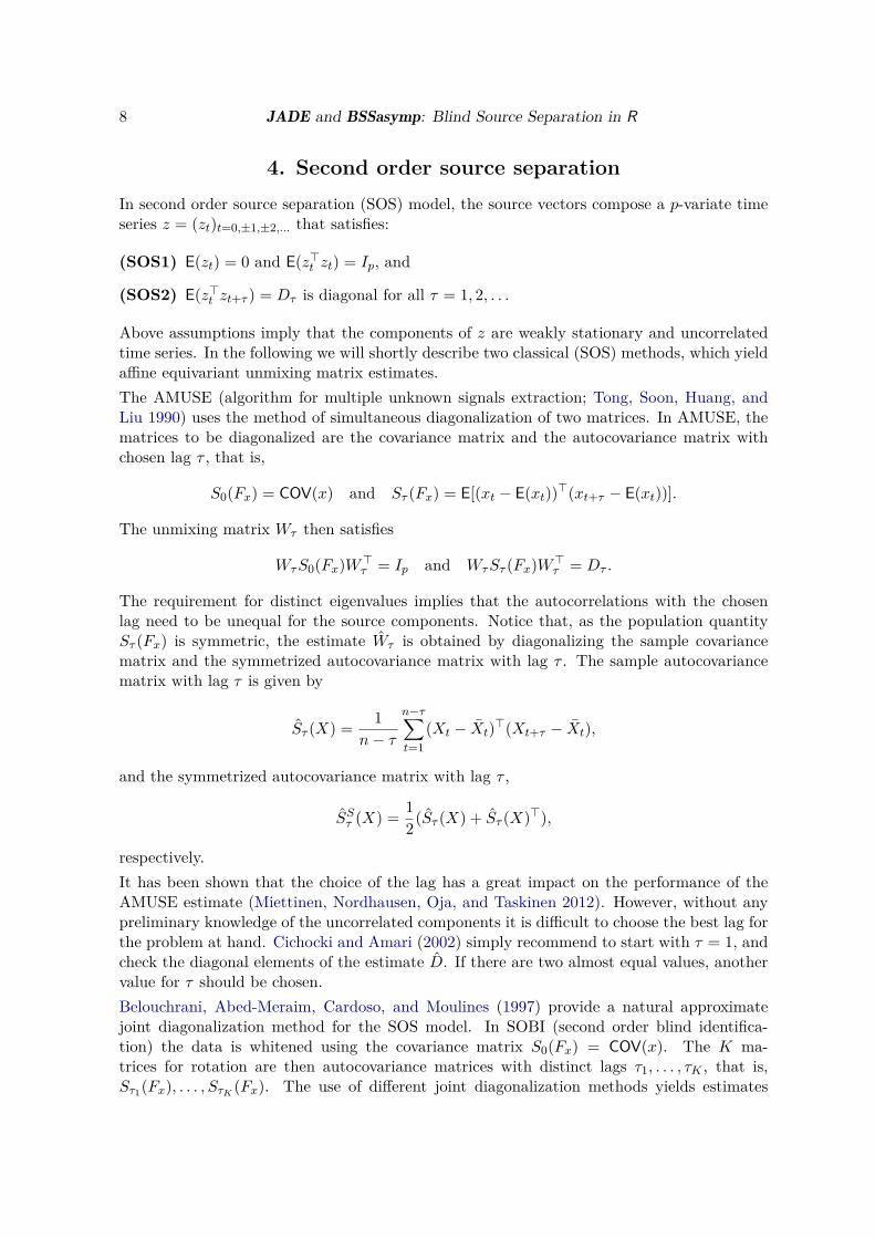
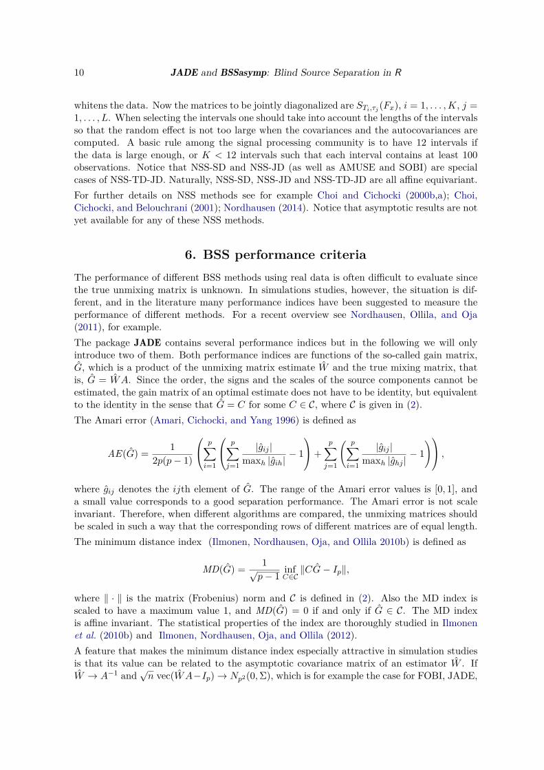
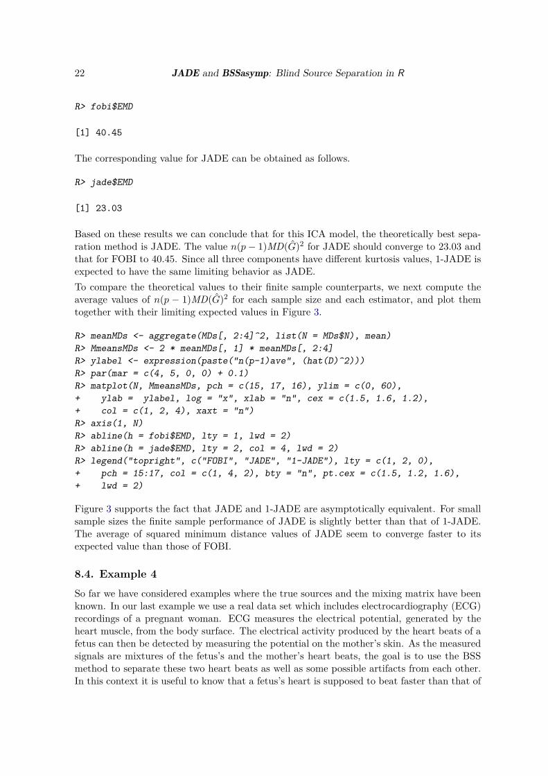
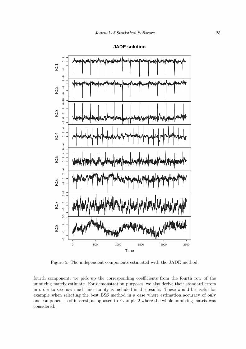X = [xgt1 xgtn ]gt such that zi = (xi minus micro)Wgt i = 1 n Notice that BSS can also beapplied in cases where the dimension of x is larger than that of z by applying a dimensionreduction method as a first stage In this paper we however restrict to the case where A isa square matrixThe unmixing matrix W cannot be estimated without further assumptions on the modelThere are three major BSS models which differ in their assumptions made upon z In inde-pendent component analysis (ICA) which is the most popular BSS approach it is assumedthat the components of z are mutually independent and at most one of them is GaussianICA applies best to cases where also z1 zn are independent and identically distributed(iid) The two other main BSS models the second order source separation (SOS) modeland the second order nonstationary source separation (NSS) model utilize temporal or spa-tial dependence within each component In the SOS model the components are assumed tobe uncorrelated weakly (second-order) stationary time series with different time dependencestructures The NSS model differs from the SOS model in that the variances of the time seriescomponents are allowed to be nonstationary All these three models will be defined in detaillater in this paperNone of the three models has a unique solution This can be seen by choosing any p times pmatrix C from the set

C = C each row and column of C has exactly one non-zero element (2)

Then C is invertible Alowast = ACminus1 is of full rank the components of zlowast = zCgt are uncorrelated(and independent in ICA) and the model can be rewritten as x = zlowastAlowast

gt Thus the ordersigns and scales of the source components cannot be determined This means that for anygiven unmixing matrix W also W lowast = CW with C isin C is a solutionAs the scales of the latent components are not identifiable one may simply assume thatCOV(z) = Ip Let then Σ = COV(x) = AAgt denote the covariance matrix of x and furtherlet Σminus12 be the symmetric matrix satisfying Σminus12Σminus12 = Σminus1 Then for the standardizedrandom variable xst = (xminus micro)Σminus12 we have that z = xstU

gt for some orthogonal U (Mietti-nen Taskinen Nordhausen and Oja 2015b Theorem 1) Thus the search for the unmixingmatrix W can be separated into finding the whitening (standardization) matrix Σminus12 andthe rotation matrix U The unmixing matrix is then given by W = UΣminus12In this paper we describe the R package JADE (Nordhausen Cardoso Miettinen Oja Ollilaand Taskinen 2017) which offers several BSS methods covering all three major BSS modelsIn all of these methods the whitening step is performed using the regular covariance matrixwhereas the rotation matrix U is found via joint diagonalization The concepts of simul-taneous and approximate joint diagonalization are recalled in Section 2 and several ICASOS and NSS methods based on diagonalization are described in Sections 3 4 and 5 respec-tively As performance indices are widely used to compare different BSS algorithms we definesome popular indices in Section 6 We also introduce the R package BSSasymp (MiettinenNordhausen Oja and Taskinen 2017) which includes functions for computing the asymptoticcovariance matrices and their data-based estimates for most of the BSS estimators in thepackage JADE Section 7 describes the R packages JADE and BSSasymp and in Section 8we illustrate the use of these packages via simulated and real data examples






gt = D


S1Vgt = V gtΛ1



1 V



1 )gt)Ugt = UgtΛ2





Ksumk=1

M(WSkWgt)



(V )2ij










Ksumk=2

sumi 6=j

(USlowastkUgt)2ij



Ksumk=2

psumi=1



G(i j θ) =












psumj=1

Ksumk=2



Ksumk=2





Ksumk=2














the fourth moments







33 JADE




psumi=1















nminusτsumt=1



SSτ (X) = 12(Sτ (X) + Sτ (X)gt)










sumtisinT







psumi=1

psumj=1

|gij |maxh |gih|

minus 1

+psumj=1

( psumi=1

|gij |maxh |ghj |

minus 1)



CisinCCGminus Ip






) (6)






















81 Example 1







[1] [2] [3] [4][1] 01989 0066042 07960 04074[2] 03164 0007432 04714 07280[3] 01746 0294247 03068 01702[4] 07911 0476462 01509 06219














Rgt sobi

W [1] [2] [3] [4]

[1] 1931 -09493 -02541 -008017[2] -2717 11377 58263 -114549


[3] -3093 29244 47697 -270582[4] -2709 33365 24661 -119771

k [1] 1 2 3 4 5 6 7 8 9 10 11 12

method [1] frjd





[1] [2] [3] [4][1] -00241 00075 09995 00026[2] -00690 09976 -00115 00004[3] -09973 -00683 -00283 -00025[4] 00002 00009 -00074 10000








82 Example 2


(i) 1 (AMUSE)

(ii) 1ndash3

(iii) 1ndash12

(iv) 1 2 5 10 20

(iv) 1ndash50

(v) 1ndash20 25 30 100

(vi) 11ndash50







(i) (ii) (iii) (iv) (v) (vi) (vii)[1] 363 01282 01362 008217 00756 006798 01268

Rgt MDs

(i) (ii) (iii) (iv) (v) (vi) (vii)[1] 0433 003659 006072 003372 001242 001231 00121


83 Example 3












Rgt fobi$W

[1] [2] [3][1] 1 0 0[2] 0 0 1[3] 0 1 0


Rgt fobi$COV_W

[1] [2] [3] [4] [5] [6] [7] [8] [9][1] 2 0000 0000 0000 0000 00 0000 00 0000[2] 0 6189 0000 0000 0000 00 -4689 00 0000[3] 0 0000 4217 -3037 0000 00 0000 00 0000[4] 0 0000 -3037 3550 0000 00 0000 00 0000[5] 0 0000 0000 0000 11151 00 0000 00 2349[6] 0 0000 0000 0000 0000 02 0000 00 0000[7] 0 -4689 0000 0000 0000 00 5189 00 0000[8] 0 0000 0000 0000 0000 00 0000 05 0000[9] 0 0000 0000 0000 2349 00 0000 00 10151



Rgt fobi$EMD

[1] 4045


Rgt jade$EMD

[1] 2303




84 Example 4



010

2030

4050

60

n

n(pminus

1)av

e(D

2 )

250 500 1000 2000 4000 8000 16000 32000

FOBIJADE1minusJADE




Read 22500 items




minus4

02

4

Ser

ies

1

minus2

02

46

Ser

ies

2

minus6

minus2

02

Ser

ies

3

minus6

minus2

02

Ser

ies

4

minus6

minus2

02

Ser

ies

5

minus6

minus2

02

Ser

ies

6

minus2

02

46

Ser

ies

7

minus2

02

46

0 500 1000 1500 2000 2500

Ser

ies

8

Time

Data





minus8

minus4

02

IC1

minus10

minus6

minus2

2

IC2

minus2

02

46

IC3

minus4

02

4

IC4

minus4

02

46

IC5

minus6

minus2

02

IC6

minus3

minus1

13

IC7

minus3

minus1

13

0 500 1000 1500 2000 2500

IC8

Time

JADE solution





[1] 058797 074451 -191649 -001493 335648 -026278 078499 018756

Rgt SDs

[1] 007210 015221 010519 003859 014785 009713 026431 017951



[1][1] 898


[1] lt2e-16






References
























































Introduction






FOBI

JADE





Examples

Example 1

Example 2

Example 3

Example 4

Conclusions






gt = D


S1Vgt = V gtΛ1



1 V



1 )gt)Ugt = UgtΛ2





Ksumk=1

M(WSkWgt)



(V )2ij










Ksumk=2

sumi 6=j

(USlowastkUgt)2ij



Ksumk=2

psumi=1



G(i j θ) =












psumj=1

Ksumk=2



Ksumk=2





Ksumk=2














the fourth moments







33 JADE




psumi=1















nminusτsumt=1



SSτ (X) = 12(Sτ (X) + Sτ (X)gt)










sumtisinT







psumi=1

psumj=1

|gij |maxh |gih|

minus 1

+psumj=1

( psumi=1

|gij |maxh |ghj |

minus 1)



CisinCCGminus Ip






) (6)






















81 Example 1







[1] [2] [3] [4][1] 01989 0066042 07960 04074[2] 03164 0007432 04714 07280[3] 01746 0294247 03068 01702[4] 07911 0476462 01509 06219














Rgt sobi

W [1] [2] [3] [4]

[1] 1931 -09493 -02541 -008017[2] -2717 11377 58263 -114549


[3] -3093 29244 47697 -270582[4] -2709 33365 24661 -119771

k [1] 1 2 3 4 5 6 7 8 9 10 11 12

method [1] frjd





[1] [2] [3] [4][1] -00241 00075 09995 00026[2] -00690 09976 -00115 00004[3] -09973 -00683 -00283 -00025[4] 00002 00009 -00074 10000








82 Example 2


(i) 1 (AMUSE)

(ii) 1ndash3

(iii) 1ndash12

(iv) 1 2 5 10 20

(iv) 1ndash50

(v) 1ndash20 25 30 100

(vi) 11ndash50







(i) (ii) (iii) (iv) (v) (vi) (vii)[1] 363 01282 01362 008217 00756 006798 01268

Rgt MDs

(i) (ii) (iii) (iv) (v) (vi) (vii)[1] 0433 003659 006072 003372 001242 001231 00121


83 Example 3












Rgt fobi$W

[1] [2] [3][1] 1 0 0[2] 0 0 1[3] 0 1 0


Rgt fobi$COV_W

[1] [2] [3] [4] [5] [6] [7] [8] [9][1] 2 0000 0000 0000 0000 00 0000 00 0000[2] 0 6189 0000 0000 0000 00 -4689 00 0000[3] 0 0000 4217 -3037 0000 00 0000 00 0000[4] 0 0000 -3037 3550 0000 00 0000 00 0000[5] 0 0000 0000 0000 11151 00 0000 00 2349[6] 0 0000 0000 0000 0000 02 0000 00 0000[7] 0 -4689 0000 0000 0000 00 5189 00 0000[8] 0 0000 0000 0000 0000 00 0000 05 0000[9] 0 0000 0000 0000 2349 00 0000 00 10151



Rgt fobi$EMD

[1] 4045


Rgt jade$EMD

[1] 2303




84 Example 4



010

2030

4050

60

n

n(pminus

1)av

e(D

2 )

250 500 1000 2000 4000 8000 16000 32000

FOBIJADE1minusJADE




Read 22500 items




minus4

02

4

Ser

ies

1

minus2

02

46

Ser

ies

2

minus6

minus2

02

Ser

ies

3

minus6

minus2

02

Ser

ies

4

minus6

minus2

02

Ser

ies

5

minus6

minus2

02

Ser

ies

6

minus2

02

46

Ser

ies

7

minus2

02

46

0 500 1000 1500 2000 2500

Ser

ies

8

Time

Data





minus8

minus4

02

IC1

minus10

minus6

minus2

2

IC2

minus2

02

46

IC3

minus4

02

4

IC4

minus4

02

46

IC5

minus6

minus2

02

IC6

minus3

minus1

13

IC7

minus3

minus1

13

0 500 1000 1500 2000 2500

IC8

Time

JADE solution





[1] 058797 074451 -191649 -001493 335648 -026278 078499 018756

Rgt SDs

[1] 007210 015221 010519 003859 014785 009713 026431 017951



[1][1] 898


[1] lt2e-16






References
























































Introduction






FOBI

JADE





Examples

Example 1

Example 2

Example 3

Example 4

Conclusions







Ksumk=2

sumi 6=j

(USlowastkUgt)2ij



Ksumk=2

psumi=1



G(i j θ) =












psumj=1

Ksumk=2



Ksumk=2





Ksumk=2














the fourth moments







33 JADE




psumi=1















nminusτsumt=1



SSτ (X) = 12(Sτ (X) + Sτ (X)gt)










sumtisinT







psumi=1

psumj=1

|gij |maxh |gih|

minus 1

+psumj=1

( psumi=1

|gij |maxh |ghj |

minus 1)



CisinCCGminus Ip






) (6)






















81 Example 1







[1] [2] [3] [4][1] 01989 0066042 07960 04074[2] 03164 0007432 04714 07280[3] 01746 0294247 03068 01702[4] 07911 0476462 01509 06219














Rgt sobi

W [1] [2] [3] [4]

[1] 1931 -09493 -02541 -008017[2] -2717 11377 58263 -114549


[3] -3093 29244 47697 -270582[4] -2709 33365 24661 -119771

k [1] 1 2 3 4 5 6 7 8 9 10 11 12

method [1] frjd





[1] [2] [3] [4][1] -00241 00075 09995 00026[2] -00690 09976 -00115 00004[3] -09973 -00683 -00283 -00025[4] 00002 00009 -00074 10000








82 Example 2


(i) 1 (AMUSE)

(ii) 1ndash3

(iii) 1ndash12

(iv) 1 2 5 10 20

(iv) 1ndash50

(v) 1ndash20 25 30 100

(vi) 11ndash50







(i) (ii) (iii) (iv) (v) (vi) (vii)[1] 363 01282 01362 008217 00756 006798 01268

Rgt MDs

(i) (ii) (iii) (iv) (v) (vi) (vii)[1] 0433 003659 006072 003372 001242 001231 00121


83 Example 3












Rgt fobi$W

[1] [2] [3][1] 1 0 0[2] 0 0 1[3] 0 1 0


Rgt fobi$COV_W

[1] [2] [3] [4] [5] [6] [7] [8] [9][1] 2 0000 0000 0000 0000 00 0000 00 0000[2] 0 6189 0000 0000 0000 00 -4689 00 0000[3] 0 0000 4217 -3037 0000 00 0000 00 0000[4] 0 0000 -3037 3550 0000 00 0000 00 0000[5] 0 0000 0000 0000 11151 00 0000 00 2349[6] 0 0000 0000 0000 0000 02 0000 00 0000[7] 0 -4689 0000 0000 0000 00 5189 00 0000[8] 0 0000 0000 0000 0000 00 0000 05 0000[9] 0 0000 0000 0000 2349 00 0000 00 10151



Rgt fobi$EMD

[1] 4045


Rgt jade$EMD

[1] 2303




84 Example 4



010

2030

4050

60

n

n(pminus

1)av

e(D

2 )

250 500 1000 2000 4000 8000 16000 32000

FOBIJADE1minusJADE




Read 22500 items




minus4

02

4

Ser

ies

1

minus2

02

46

Ser

ies

2

minus6

minus2

02

Ser

ies

3

minus6

minus2

02

Ser

ies

4

minus6

minus2

02

Ser

ies

5

minus6

minus2

02

Ser

ies

6

minus2

02

46

Ser

ies

7

minus2

02

46

0 500 1000 1500 2000 2500

Ser

ies

8

Time

Data





minus8

minus4

02

IC1

minus10

minus6

minus2

2

IC2

minus2

02

46

IC3

minus4

02

4

IC4

minus4

02

46

IC5

minus6

minus2

02

IC6

minus3

minus1

13

IC7

minus3

minus1

13

0 500 1000 1500 2000 2500

IC8

Time

JADE solution





[1] 058797 074451 -191649 -001493 335648 -026278 078499 018756

Rgt SDs

[1] 007210 015221 010519 003859 014785 009713 026431 017951



[1][1] 898


[1] lt2e-16






References
























































Introduction






FOBI

JADE





Examples

Example 1

Example 2

Example 3

Example 4

Conclusions




psumj=1

Ksumk=2



Ksumk=2





Ksumk=2














the fourth moments







33 JADE




psumi=1















nminusτsumt=1



SSτ (X) = 12(Sτ (X) + Sτ (X)gt)










sumtisinT







psumi=1

psumj=1

|gij |maxh |gih|

minus 1

+psumj=1

( psumi=1

|gij |maxh |ghj |

minus 1)



CisinCCGminus Ip






) (6)






















81 Example 1







[1] [2] [3] [4][1] 01989 0066042 07960 04074[2] 03164 0007432 04714 07280[3] 01746 0294247 03068 01702[4] 07911 0476462 01509 06219














Rgt sobi

W [1] [2] [3] [4]

[1] 1931 -09493 -02541 -008017[2] -2717 11377 58263 -114549


[3] -3093 29244 47697 -270582[4] -2709 33365 24661 -119771

k [1] 1 2 3 4 5 6 7 8 9 10 11 12

method [1] frjd





[1] [2] [3] [4][1] -00241 00075 09995 00026[2] -00690 09976 -00115 00004[3] -09973 -00683 -00283 -00025[4] 00002 00009 -00074 10000








82 Example 2


(i) 1 (AMUSE)

(ii) 1ndash3

(iii) 1ndash12

(iv) 1 2 5 10 20

(iv) 1ndash50

(v) 1ndash20 25 30 100

(vi) 11ndash50







(i) (ii) (iii) (iv) (v) (vi) (vii)[1] 363 01282 01362 008217 00756 006798 01268

Rgt MDs

(i) (ii) (iii) (iv) (v) (vi) (vii)[1] 0433 003659 006072 003372 001242 001231 00121


83 Example 3












Rgt fobi$W

[1] [2] [3][1] 1 0 0[2] 0 0 1[3] 0 1 0


Rgt fobi$COV_W

[1] [2] [3] [4] [5] [6] [7] [8] [9][1] 2 0000 0000 0000 0000 00 0000 00 0000[2] 0 6189 0000 0000 0000 00 -4689 00 0000[3] 0 0000 4217 -3037 0000 00 0000 00 0000[4] 0 0000 -3037 3550 0000 00 0000 00 0000[5] 0 0000 0000 0000 11151 00 0000 00 2349[6] 0 0000 0000 0000 0000 02 0000 00 0000[7] 0 -4689 0000 0000 0000 00 5189 00 0000[8] 0 0000 0000 0000 0000 00 0000 05 0000[9] 0 0000 0000 0000 2349 00 0000 00 10151



Rgt fobi$EMD

[1] 4045


Rgt jade$EMD

[1] 2303




84 Example 4



010

2030

4050

60

n

n(pminus

1)av

e(D

2 )

250 500 1000 2000 4000 8000 16000 32000

FOBIJADE1minusJADE




Read 22500 items




minus4

02

4

Ser

ies

1

minus2

02

46

Ser

ies

2

minus6

minus2

02

Ser

ies

3

minus6

minus2

02

Ser

ies

4

minus6

minus2

02

Ser

ies

5

minus6

minus2

02

Ser

ies

6

minus2

02

46

Ser

ies

7

minus2

02

46

0 500 1000 1500 2000 2500

Ser

ies

8

Time

Data





minus8

minus4

02

IC1

minus10

minus6

minus2

2

IC2

minus2

02

46

IC3

minus4

02

4

IC4

minus4

02

46

IC5

minus6

minus2

02

IC6

minus3

minus1

13

IC7

minus3

minus1

13

0 500 1000 1500 2000 2500

IC8

Time

JADE solution





[1] 058797 074451 -191649 -001493 335648 -026278 078499 018756

Rgt SDs

[1] 007210 015221 010519 003859 014785 009713 026431 017951



[1][1] 898


[1] lt2e-16






References
























































Introduction






FOBI

JADE





Examples

Example 1

Example 2

Example 3

Example 4

Conclusions








the fourth moments







33 JADE




psumi=1















nminusτsumt=1



SSτ (X) = 12(Sτ (X) + Sτ (X)gt)










sumtisinT







psumi=1

psumj=1

|gij |maxh |gih|

minus 1

+psumj=1

( psumi=1

|gij |maxh |ghj |

minus 1)



CisinCCGminus Ip






) (6)






















81 Example 1







[1] [2] [3] [4][1] 01989 0066042 07960 04074[2] 03164 0007432 04714 07280[3] 01746 0294247 03068 01702[4] 07911 0476462 01509 06219














Rgt sobi

W [1] [2] [3] [4]

[1] 1931 -09493 -02541 -008017[2] -2717 11377 58263 -114549


[3] -3093 29244 47697 -270582[4] -2709 33365 24661 -119771

k [1] 1 2 3 4 5 6 7 8 9 10 11 12

method [1] frjd





[1] [2] [3] [4][1] -00241 00075 09995 00026[2] -00690 09976 -00115 00004[3] -09973 -00683 -00283 -00025[4] 00002 00009 -00074 10000








82 Example 2


(i) 1 (AMUSE)

(ii) 1ndash3

(iii) 1ndash12

(iv) 1 2 5 10 20

(iv) 1ndash50

(v) 1ndash20 25 30 100

(vi) 11ndash50







(i) (ii) (iii) (iv) (v) (vi) (vii)[1] 363 01282 01362 008217 00756 006798 01268

Rgt MDs

(i) (ii) (iii) (iv) (v) (vi) (vii)[1] 0433 003659 006072 003372 001242 001231 00121


83 Example 3












Rgt fobi$W

[1] [2] [3][1] 1 0 0[2] 0 0 1[3] 0 1 0


Rgt fobi$COV_W

[1] [2] [3] [4] [5] [6] [7] [8] [9][1] 2 0000 0000 0000 0000 00 0000 00 0000[2] 0 6189 0000 0000 0000 00 -4689 00 0000[3] 0 0000 4217 -3037 0000 00 0000 00 0000[4] 0 0000 -3037 3550 0000 00 0000 00 0000[5] 0 0000 0000 0000 11151 00 0000 00 2349[6] 0 0000 0000 0000 0000 02 0000 00 0000[7] 0 -4689 0000 0000 0000 00 5189 00 0000[8] 0 0000 0000 0000 0000 00 0000 05 0000[9] 0 0000 0000 0000 2349 00 0000 00 10151



Rgt fobi$EMD

[1] 4045


Rgt jade$EMD

[1] 2303




84 Example 4



010

2030

4050

60

n

n(pminus

1)av

e(D

2 )

250 500 1000 2000 4000 8000 16000 32000

FOBIJADE1minusJADE




Read 22500 items




minus4

02

4

Ser

ies

1

minus2

02

46

Ser

ies

2

minus6

minus2

02

Ser

ies

3

minus6

minus2

02

Ser

ies

4

minus6

minus2

02

Ser

ies

5

minus6

minus2

02

Ser

ies

6

minus2

02

46

Ser

ies

7

minus2

02

46

0 500 1000 1500 2000 2500

Ser

ies

8

Time

Data





minus8

minus4

02

IC1

minus10

minus6

minus2

2

IC2

minus2

02

46

IC3

minus4

02

4

IC4

minus4

02

46

IC5

minus6

minus2

02

IC6

minus3

minus1

13

IC7

minus3

minus1

13

0 500 1000 1500 2000 2500

IC8

Time

JADE solution





[1] 058797 074451 -191649 -001493 335648 -026278 078499 018756

Rgt SDs

[1] 007210 015221 010519 003859 014785 009713 026431 017951



[1][1] 898


[1] lt2e-16






References
























































Introduction






FOBI

JADE





Examples

Example 1

Example 2

Example 3

Example 4

Conclusions











nminusτsumt=1



SSτ (X) = 12(Sτ (X) + Sτ (X)gt)










sumtisinT







psumi=1

psumj=1

|gij |maxh |gih|

minus 1

+psumj=1

( psumi=1

|gij |maxh |ghj |

minus 1)



CisinCCGminus Ip






) (6)






















81 Example 1







[1] [2] [3] [4][1] 01989 0066042 07960 04074[2] 03164 0007432 04714 07280[3] 01746 0294247 03068 01702[4] 07911 0476462 01509 06219














Rgt sobi

W [1] [2] [3] [4]

[1] 1931 -09493 -02541 -008017[2] -2717 11377 58263 -114549


[3] -3093 29244 47697 -270582[4] -2709 33365 24661 -119771

k [1] 1 2 3 4 5 6 7 8 9 10 11 12

method [1] frjd





[1] [2] [3] [4][1] -00241 00075 09995 00026[2] -00690 09976 -00115 00004[3] -09973 -00683 -00283 -00025[4] 00002 00009 -00074 10000








82 Example 2


(i) 1 (AMUSE)

(ii) 1ndash3

(iii) 1ndash12

(iv) 1 2 5 10 20

(iv) 1ndash50

(v) 1ndash20 25 30 100

(vi) 11ndash50







(i) (ii) (iii) (iv) (v) (vi) (vii)[1] 363 01282 01362 008217 00756 006798 01268

Rgt MDs

(i) (ii) (iii) (iv) (v) (vi) (vii)[1] 0433 003659 006072 003372 001242 001231 00121


83 Example 3












Rgt fobi$W

[1] [2] [3][1] 1 0 0[2] 0 0 1[3] 0 1 0


Rgt fobi$COV_W

[1] [2] [3] [4] [5] [6] [7] [8] [9][1] 2 0000 0000 0000 0000 00 0000 00 0000[2] 0 6189 0000 0000 0000 00 -4689 00 0000[3] 0 0000 4217 -3037 0000 00 0000 00 0000[4] 0 0000 -3037 3550 0000 00 0000 00 0000[5] 0 0000 0000 0000 11151 00 0000 00 2349[6] 0 0000 0000 0000 0000 02 0000 00 0000[7] 0 -4689 0000 0000 0000 00 5189 00 0000[8] 0 0000 0000 0000 0000 00 0000 05 0000[9] 0 0000 0000 0000 2349 00 0000 00 10151



Rgt fobi$EMD

[1] 4045


Rgt jade$EMD

[1] 2303




84 Example 4



010

2030

4050

60

n

n(pminus

1)av

e(D

2 )

250 500 1000 2000 4000 8000 16000 32000

FOBIJADE1minusJADE




Read 22500 items




minus4

02

4

Ser

ies

1

minus2

02

46

Ser

ies

2

minus6

minus2

02

Ser

ies

3

minus6

minus2

02

Ser

ies

4

minus6

minus2

02

Ser

ies

5

minus6

minus2

02

Ser

ies

6

minus2

02

46

Ser

ies

7

minus2

02

46

0 500 1000 1500 2000 2500

Ser

ies

8

Time

Data





minus8

minus4

02

IC1

minus10

minus6

minus2

2

IC2

minus2

02

46

IC3

minus4

02

4

IC4

minus4

02

46

IC5

minus6

minus2

02

IC6

minus3

minus1

13

IC7

minus3

minus1

13

0 500 1000 1500 2000 2500

IC8

Time

JADE solution





[1] 058797 074451 -191649 -001493 335648 -026278 078499 018756

Rgt SDs

[1] 007210 015221 010519 003859 014785 009713 026431 017951



[1][1] 898


[1] lt2e-16






References
























































Introduction






FOBI

JADE





Examples

Example 1

Example 2

Example 3

Example 4

Conclusions









sumtisinT







psumi=1

psumj=1

|gij |maxh |gih|

minus 1

+psumj=1

( psumi=1

|gij |maxh |ghj |

minus 1)



CisinCCGminus Ip






) (6)






















81 Example 1







[1] [2] [3] [4][1] 01989 0066042 07960 04074[2] 03164 0007432 04714 07280[3] 01746 0294247 03068 01702[4] 07911 0476462 01509 06219














Rgt sobi

W [1] [2] [3] [4]

[1] 1931 -09493 -02541 -008017[2] -2717 11377 58263 -114549


[3] -3093 29244 47697 -270582[4] -2709 33365 24661 -119771

k [1] 1 2 3 4 5 6 7 8 9 10 11 12

method [1] frjd





[1] [2] [3] [4][1] -00241 00075 09995 00026[2] -00690 09976 -00115 00004[3] -09973 -00683 -00283 -00025[4] 00002 00009 -00074 10000








82 Example 2


(i) 1 (AMUSE)

(ii) 1ndash3

(iii) 1ndash12

(iv) 1 2 5 10 20

(iv) 1ndash50

(v) 1ndash20 25 30 100

(vi) 11ndash50







(i) (ii) (iii) (iv) (v) (vi) (vii)[1] 363 01282 01362 008217 00756 006798 01268

Rgt MDs

(i) (ii) (iii) (iv) (v) (vi) (vii)[1] 0433 003659 006072 003372 001242 001231 00121


83 Example 3












Rgt fobi$W

[1] [2] [3][1] 1 0 0[2] 0 0 1[3] 0 1 0


Rgt fobi$COV_W

[1] [2] [3] [4] [5] [6] [7] [8] [9][1] 2 0000 0000 0000 0000 00 0000 00 0000[2] 0 6189 0000 0000 0000 00 -4689 00 0000[3] 0 0000 4217 -3037 0000 00 0000 00 0000[4] 0 0000 -3037 3550 0000 00 0000 00 0000[5] 0 0000 0000 0000 11151 00 0000 00 2349[6] 0 0000 0000 0000 0000 02 0000 00 0000[7] 0 -4689 0000 0000 0000 00 5189 00 0000[8] 0 0000 0000 0000 0000 00 0000 05 0000[9] 0 0000 0000 0000 2349 00 0000 00 10151



Rgt fobi$EMD

[1] 4045


Rgt jade$EMD

[1] 2303




84 Example 4



010

2030

4050

60

n

n(pminus

1)av

e(D

2 )

250 500 1000 2000 4000 8000 16000 32000

FOBIJADE1minusJADE




Read 22500 items




minus4

02

4

Ser

ies

1

minus2

02

46

Ser

ies

2

minus6

minus2

02

Ser

ies

3

minus6

minus2

02

Ser

ies

4

minus6

minus2

02

Ser

ies

5

minus6

minus2

02

Ser

ies

6

minus2

02

46

Ser

ies

7

minus2

02

46

0 500 1000 1500 2000 2500

Ser

ies

8

Time

Data





minus8

minus4

02

IC1

minus10

minus6

minus2

2

IC2

minus2

02

46

IC3

minus4

02

4

IC4

minus4

02

46

IC5

minus6

minus2

02

IC6

minus3

minus1

13

IC7

minus3

minus1

13

0 500 1000 1500 2000 2500

IC8

Time

JADE solution





[1] 058797 074451 -191649 -001493 335648 -026278 078499 018756

Rgt SDs

[1] 007210 015221 010519 003859 014785 009713 026431 017951



[1][1] 898


[1] lt2e-16






References
























































Introduction






FOBI

JADE





Examples

Example 1

Example 2

Example 3

Example 4

Conclusions





psumi=1

psumj=1

|gij |maxh |gih|

minus 1

+psumj=1

( psumi=1

|gij |maxh |ghj |

minus 1)



CisinCCGminus Ip






) (6)






















81 Example 1







[1] [2] [3] [4][1] 01989 0066042 07960 04074[2] 03164 0007432 04714 07280[3] 01746 0294247 03068 01702[4] 07911 0476462 01509 06219














Rgt sobi

W [1] [2] [3] [4]

[1] 1931 -09493 -02541 -008017[2] -2717 11377 58263 -114549


[3] -3093 29244 47697 -270582[4] -2709 33365 24661 -119771

k [1] 1 2 3 4 5 6 7 8 9 10 11 12

method [1] frjd





[1] [2] [3] [4][1] -00241 00075 09995 00026[2] -00690 09976 -00115 00004[3] -09973 -00683 -00283 -00025[4] 00002 00009 -00074 10000








82 Example 2


(i) 1 (AMUSE)

(ii) 1ndash3

(iii) 1ndash12

(iv) 1 2 5 10 20

(iv) 1ndash50

(v) 1ndash20 25 30 100

(vi) 11ndash50







(i) (ii) (iii) (iv) (v) (vi) (vii)[1] 363 01282 01362 008217 00756 006798 01268

Rgt MDs

(i) (ii) (iii) (iv) (v) (vi) (vii)[1] 0433 003659 006072 003372 001242 001231 00121


83 Example 3












Rgt fobi$W

[1] [2] [3][1] 1 0 0[2] 0 0 1[3] 0 1 0


Rgt fobi$COV_W

[1] [2] [3] [4] [5] [6] [7] [8] [9][1] 2 0000 0000 0000 0000 00 0000 00 0000[2] 0 6189 0000 0000 0000 00 -4689 00 0000[3] 0 0000 4217 -3037 0000 00 0000 00 0000[4] 0 0000 -3037 3550 0000 00 0000 00 0000[5] 0 0000 0000 0000 11151 00 0000 00 2349[6] 0 0000 0000 0000 0000 02 0000 00 0000[7] 0 -4689 0000 0000 0000 00 5189 00 0000[8] 0 0000 0000 0000 0000 00 0000 05 0000[9] 0 0000 0000 0000 2349 00 0000 00 10151



Rgt fobi$EMD

[1] 4045


Rgt jade$EMD

[1] 2303




84 Example 4



010

2030

4050

60

n

n(pminus

1)av

e(D

2 )

250 500 1000 2000 4000 8000 16000 32000

FOBIJADE1minusJADE




Read 22500 items




minus4

02

4

Ser

ies

1

minus2

02

46

Ser

ies

2

minus6

minus2

02

Ser

ies

3

minus6

minus2

02

Ser

ies

4

minus6

minus2

02

Ser

ies

5

minus6

minus2

02

Ser

ies

6

minus2

02

46

Ser

ies

7

minus2

02

46

0 500 1000 1500 2000 2500

Ser

ies

8

Time

Data





minus8

minus4

02

IC1

minus10

minus6

minus2

2

IC2

minus2

02

46

IC3

minus4

02

4

IC4

minus4

02

46

IC5

minus6

minus2

02

IC6

minus3

minus1

13

IC7

minus3

minus1

13

0 500 1000 1500 2000 2500

IC8

Time

JADE solution





[1] 058797 074451 -191649 -001493 335648 -026278 078499 018756

Rgt SDs

[1] 007210 015221 010519 003859 014785 009713 026431 017951



[1][1] 898


[1] lt2e-16






References
























































Introduction






FOBI

JADE





Examples

Example 1

Example 2

Example 3

Example 4

Conclusions




) (6)






















81 Example 1







[1] [2] [3] [4][1] 01989 0066042 07960 04074[2] 03164 0007432 04714 07280[3] 01746 0294247 03068 01702[4] 07911 0476462 01509 06219














Rgt sobi

W [1] [2] [3] [4]

[1] 1931 -09493 -02541 -008017[2] -2717 11377 58263 -114549


[3] -3093 29244 47697 -270582[4] -2709 33365 24661 -119771

k [1] 1 2 3 4 5 6 7 8 9 10 11 12

method [1] frjd





[1] [2] [3] [4][1] -00241 00075 09995 00026[2] -00690 09976 -00115 00004[3] -09973 -00683 -00283 -00025[4] 00002 00009 -00074 10000








82 Example 2


(i) 1 (AMUSE)

(ii) 1ndash3

(iii) 1ndash12

(iv) 1 2 5 10 20

(iv) 1ndash50

(v) 1ndash20 25 30 100

(vi) 11ndash50







(i) (ii) (iii) (iv) (v) (vi) (vii)[1] 363 01282 01362 008217 00756 006798 01268

Rgt MDs

(i) (ii) (iii) (iv) (v) (vi) (vii)[1] 0433 003659 006072 003372 001242 001231 00121


83 Example 3












Rgt fobi$W

[1] [2] [3][1] 1 0 0[2] 0 0 1[3] 0 1 0


Rgt fobi$COV_W

[1] [2] [3] [4] [5] [6] [7] [8] [9][1] 2 0000 0000 0000 0000 00 0000 00 0000[2] 0 6189 0000 0000 0000 00 -4689 00 0000[3] 0 0000 4217 -3037 0000 00 0000 00 0000[4] 0 0000 -3037 3550 0000 00 0000 00 0000[5] 0 0000 0000 0000 11151 00 0000 00 2349[6] 0 0000 0000 0000 0000 02 0000 00 0000[7] 0 -4689 0000 0000 0000 00 5189 00 0000[8] 0 0000 0000 0000 0000 00 0000 05 0000[9] 0 0000 0000 0000 2349 00 0000 00 10151



Rgt fobi$EMD

[1] 4045


Rgt jade$EMD

[1] 2303




84 Example 4



010

2030

4050

60

n

n(pminus

1)av

e(D

2 )

250 500 1000 2000 4000 8000 16000 32000

FOBIJADE1minusJADE




Read 22500 items




minus4

02

4

Ser

ies

1

minus2

02

46

Ser

ies

2

minus6

minus2

02

Ser

ies

3

minus6

minus2

02

Ser

ies

4

minus6

minus2

02

Ser

ies

5

minus6

minus2

02

Ser

ies

6

minus2

02

46

Ser

ies

7

minus2

02

46

0 500 1000 1500 2000 2500

Ser

ies

8

Time

Data





minus8

minus4

02

IC1

minus10

minus6

minus2

2

IC2

minus2

02

46

IC3

minus4

02

4

IC4

minus4

02

46

IC5

minus6

minus2

02

IC6

minus3

minus1

13

IC7

minus3

minus1

13

0 500 1000 1500 2000 2500

IC8

Time

JADE solution





[1] 058797 074451 -191649 -001493 335648 -026278 078499 018756

Rgt SDs

[1] 007210 015221 010519 003859 014785 009713 026431 017951



[1][1] 898


[1] lt2e-16






References
























































Introduction






FOBI

JADE





Examples

Example 1

Example 2

Example 3

Example 4

Conclusions







81 Example 1







[1] [2] [3] [4][1] 01989 0066042 07960 04074[2] 03164 0007432 04714 07280[3] 01746 0294247 03068 01702[4] 07911 0476462 01509 06219














Rgt sobi

W [1] [2] [3] [4]

[1] 1931 -09493 -02541 -008017[2] -2717 11377 58263 -114549


[3] -3093 29244 47697 -270582[4] -2709 33365 24661 -119771

k [1] 1 2 3 4 5 6 7 8 9 10 11 12

method [1] frjd





[1] [2] [3] [4][1] -00241 00075 09995 00026[2] -00690 09976 -00115 00004[3] -09973 -00683 -00283 -00025[4] 00002 00009 -00074 10000








82 Example 2


(i) 1 (AMUSE)

(ii) 1ndash3

(iii) 1ndash12

(iv) 1 2 5 10 20

(iv) 1ndash50

(v) 1ndash20 25 30 100

(vi) 11ndash50







(i) (ii) (iii) (iv) (v) (vi) (vii)[1] 363 01282 01362 008217 00756 006798 01268

Rgt MDs

(i) (ii) (iii) (iv) (v) (vi) (vii)[1] 0433 003659 006072 003372 001242 001231 00121


83 Example 3












Rgt fobi$W

[1] [2] [3][1] 1 0 0[2] 0 0 1[3] 0 1 0


Rgt fobi$COV_W

[1] [2] [3] [4] [5] [6] [7] [8] [9][1] 2 0000 0000 0000 0000 00 0000 00 0000[2] 0 6189 0000 0000 0000 00 -4689 00 0000[3] 0 0000 4217 -3037 0000 00 0000 00 0000[4] 0 0000 -3037 3550 0000 00 0000 00 0000[5] 0 0000 0000 0000 11151 00 0000 00 2349[6] 0 0000 0000 0000 0000 02 0000 00 0000[7] 0 -4689 0000 0000 0000 00 5189 00 0000[8] 0 0000 0000 0000 0000 00 0000 05 0000[9] 0 0000 0000 0000 2349 00 0000 00 10151



Rgt fobi$EMD

[1] 4045


Rgt jade$EMD

[1] 2303




84 Example 4



010

2030

4050

60

n

n(pminus

1)av

e(D

2 )

250 500 1000 2000 4000 8000 16000 32000

FOBIJADE1minusJADE




Read 22500 items




minus4

02

4

Ser

ies

1

minus2

02

46

Ser

ies

2

minus6

minus2

02

Ser

ies

3

minus6

minus2

02

Ser

ies

4

minus6

minus2

02

Ser

ies

5

minus6

minus2

02

Ser

ies

6

minus2

02

46

Ser

ies

7

minus2

02

46

0 500 1000 1500 2000 2500

Ser

ies

8

Time

Data





minus8

minus4

02

IC1

minus10

minus6

minus2

2

IC2

minus2

02

46

IC3

minus4

02

4

IC4

minus4

02

46

IC5

minus6

minus2

02

IC6

minus3

minus1

13

IC7

minus3

minus1

13

0 500 1000 1500 2000 2500

IC8

Time

JADE solution





[1] 058797 074451 -191649 -001493 335648 -026278 078499 018756

Rgt SDs

[1] 007210 015221 010519 003859 014785 009713 026431 017951



[1][1] 898


[1] lt2e-16






References
























































Introduction






FOBI

JADE





Examples

Example 1

Example 2

Example 3

Example 4

Conclusions











Rgt sobi

W [1] [2] [3] [4]

[1] 1931 -09493 -02541 -008017[2] -2717 11377 58263 -114549


[3] -3093 29244 47697 -270582[4] -2709 33365 24661 -119771

k [1] 1 2 3 4 5 6 7 8 9 10 11 12

method [1] frjd





[1] [2] [3] [4][1] -00241 00075 09995 00026[2] -00690 09976 -00115 00004[3] -09973 -00683 -00283 -00025[4] 00002 00009 -00074 10000








82 Example 2


(i) 1 (AMUSE)

(ii) 1ndash3

(iii) 1ndash12

(iv) 1 2 5 10 20

(iv) 1ndash50

(v) 1ndash20 25 30 100

(vi) 11ndash50







(i) (ii) (iii) (iv) (v) (vi) (vii)[1] 363 01282 01362 008217 00756 006798 01268

Rgt MDs

(i) (ii) (iii) (iv) (v) (vi) (vii)[1] 0433 003659 006072 003372 001242 001231 00121


83 Example 3












Rgt fobi$W

[1] [2] [3][1] 1 0 0[2] 0 0 1[3] 0 1 0


Rgt fobi$COV_W

[1] [2] [3] [4] [5] [6] [7] [8] [9][1] 2 0000 0000 0000 0000 00 0000 00 0000[2] 0 6189 0000 0000 0000 00 -4689 00 0000[3] 0 0000 4217 -3037 0000 00 0000 00 0000[4] 0 0000 -3037 3550 0000 00 0000 00 0000[5] 0 0000 0000 0000 11151 00 0000 00 2349[6] 0 0000 0000 0000 0000 02 0000 00 0000[7] 0 -4689 0000 0000 0000 00 5189 00 0000[8] 0 0000 0000 0000 0000 00 0000 05 0000[9] 0 0000 0000 0000 2349 00 0000 00 10151



Rgt fobi$EMD

[1] 4045


Rgt jade$EMD

[1] 2303




84 Example 4



010

2030

4050

60

n

n(pminus

1)av

e(D

2 )

250 500 1000 2000 4000 8000 16000 32000

FOBIJADE1minusJADE




Read 22500 items




minus4

02

4

Ser

ies

1

minus2

02

46

Ser

ies

2

minus6

minus2

02

Ser

ies

3

minus6

minus2

02

Ser

ies

4

minus6

minus2

02

Ser

ies

5

minus6

minus2

02

Ser

ies

6

minus2

02

46

Ser

ies

7

minus2

02

46

0 500 1000 1500 2000 2500

Ser

ies

8

Time

Data





minus8

minus4

02

IC1

minus10

minus6

minus2

2

IC2

minus2

02

46

IC3

minus4

02

4

IC4

minus4

02

46

IC5

minus6

minus2

02

IC6

minus3

minus1

13

IC7

minus3

minus1

13

0 500 1000 1500 2000 2500

IC8

Time

JADE solution





[1] 058797 074451 -191649 -001493 335648 -026278 078499 018756

Rgt SDs

[1] 007210 015221 010519 003859 014785 009713 026431 017951



[1][1] 898


[1] lt2e-16






References
























































Introduction






FOBI

JADE





Examples

Example 1

Example 2

Example 3

Example 4

Conclusions


[3] -3093 29244 47697 -270582[4] -2709 33365 24661 -119771

k [1] 1 2 3 4 5 6 7 8 9 10 11 12

method [1] frjd





[1] [2] [3] [4][1] -00241 00075 09995 00026[2] -00690 09976 -00115 00004[3] -09973 -00683 -00283 -00025[4] 00002 00009 -00074 10000








82 Example 2


(i) 1 (AMUSE)

(ii) 1ndash3

(iii) 1ndash12

(iv) 1 2 5 10 20

(iv) 1ndash50

(v) 1ndash20 25 30 100

(vi) 11ndash50







(i) (ii) (iii) (iv) (v) (vi) (vii)[1] 363 01282 01362 008217 00756 006798 01268

Rgt MDs

(i) (ii) (iii) (iv) (v) (vi) (vii)[1] 0433 003659 006072 003372 001242 001231 00121


83 Example 3












Rgt fobi$W

[1] [2] [3][1] 1 0 0[2] 0 0 1[3] 0 1 0


Rgt fobi$COV_W

[1] [2] [3] [4] [5] [6] [7] [8] [9][1] 2 0000 0000 0000 0000 00 0000 00 0000[2] 0 6189 0000 0000 0000 00 -4689 00 0000[3] 0 0000 4217 -3037 0000 00 0000 00 0000[4] 0 0000 -3037 3550 0000 00 0000 00 0000[5] 0 0000 0000 0000 11151 00 0000 00 2349[6] 0 0000 0000 0000 0000 02 0000 00 0000[7] 0 -4689 0000 0000 0000 00 5189 00 0000[8] 0 0000 0000 0000 0000 00 0000 05 0000[9] 0 0000 0000 0000 2349 00 0000 00 10151



Rgt fobi$EMD

[1] 4045


Rgt jade$EMD

[1] 2303




84 Example 4



010

2030

4050

60

n

n(pminus

1)av

e(D

2 )

250 500 1000 2000 4000 8000 16000 32000

FOBIJADE1minusJADE




Read 22500 items




minus4

02

4

Ser

ies

1

minus2

02

46

Ser

ies

2

minus6

minus2

02

Ser

ies

3

minus6

minus2

02

Ser

ies

4

minus6

minus2

02

Ser

ies

5

minus6

minus2

02

Ser

ies

6

minus2

02

46

Ser

ies

7

minus2

02

46

0 500 1000 1500 2000 2500

Ser

ies

8

Time

Data





minus8

minus4

02

IC1

minus10

minus6

minus2

2

IC2

minus2

02

46

IC3

minus4

02

4

IC4

minus4

02

46

IC5

minus6

minus2

02

IC6

minus3

minus1

13

IC7

minus3

minus1

13

0 500 1000 1500 2000 2500

IC8

Time

JADE solution





[1] 058797 074451 -191649 -001493 335648 -026278 078499 018756

Rgt SDs

[1] 007210 015221 010519 003859 014785 009713 026431 017951



[1][1] 898


[1] lt2e-16






References
























































Introduction






FOBI

JADE





Examples

Example 1

Example 2

Example 3

Example 4

Conclusions



82 Example 2


(i) 1 (AMUSE)

(ii) 1ndash3

(iii) 1ndash12

(iv) 1 2 5 10 20

(iv) 1ndash50

(v) 1ndash20 25 30 100

(vi) 11ndash50







(i) (ii) (iii) (iv) (v) (vi) (vii)[1] 363 01282 01362 008217 00756 006798 01268

Rgt MDs

(i) (ii) (iii) (iv) (v) (vi) (vii)[1] 0433 003659 006072 003372 001242 001231 00121


83 Example 3












Rgt fobi$W

[1] [2] [3][1] 1 0 0[2] 0 0 1[3] 0 1 0


Rgt fobi$COV_W

[1] [2] [3] [4] [5] [6] [7] [8] [9][1] 2 0000 0000 0000 0000 00 0000 00 0000[2] 0 6189 0000 0000 0000 00 -4689 00 0000[3] 0 0000 4217 -3037 0000 00 0000 00 0000[4] 0 0000 -3037 3550 0000 00 0000 00 0000[5] 0 0000 0000 0000 11151 00 0000 00 2349[6] 0 0000 0000 0000 0000 02 0000 00 0000[7] 0 -4689 0000 0000 0000 00 5189 00 0000[8] 0 0000 0000 0000 0000 00 0000 05 0000[9] 0 0000 0000 0000 2349 00 0000 00 10151



Rgt fobi$EMD

[1] 4045


Rgt jade$EMD

[1] 2303




84 Example 4



010

2030

4050

60

n

n(pminus

1)av

e(D

2 )

250 500 1000 2000 4000 8000 16000 32000

FOBIJADE1minusJADE




Read 22500 items




minus4

02

4

Ser

ies

1

minus2

02

46

Ser

ies

2

minus6

minus2

02

Ser

ies

3

minus6

minus2

02

Ser

ies

4

minus6

minus2

02

Ser

ies

5

minus6

minus2

02

Ser

ies

6

minus2

02

46

Ser

ies

7

minus2

02

46

0 500 1000 1500 2000 2500

Ser

ies

8

Time

Data





minus8

minus4

02

IC1

minus10

minus6

minus2

2

IC2

minus2

02

46

IC3

minus4

02

4

IC4

minus4

02

46

IC5

minus6

minus2

02

IC6

minus3

minus1

13

IC7

minus3

minus1

13

0 500 1000 1500 2000 2500

IC8

Time

JADE solution





[1] 058797 074451 -191649 -001493 335648 -026278 078499 018756

Rgt SDs

[1] 007210 015221 010519 003859 014785 009713 026431 017951



[1][1] 898


[1] lt2e-16






References
























































Introduction






FOBI

JADE





Examples

Example 1

Example 2

Example 3

Example 4

Conclusions





(i) (ii) (iii) (iv) (v) (vi) (vii)[1] 363 01282 01362 008217 00756 006798 01268

Rgt MDs

(i) (ii) (iii) (iv) (v) (vi) (vii)[1] 0433 003659 006072 003372 001242 001231 00121


83 Example 3












Rgt fobi$W

[1] [2] [3][1] 1 0 0[2] 0 0 1[3] 0 1 0


Rgt fobi$COV_W

[1] [2] [3] [4] [5] [6] [7] [8] [9][1] 2 0000 0000 0000 0000 00 0000 00 0000[2] 0 6189 0000 0000 0000 00 -4689 00 0000[3] 0 0000 4217 -3037 0000 00 0000 00 0000[4] 0 0000 -3037 3550 0000 00 0000 00 0000[5] 0 0000 0000 0000 11151 00 0000 00 2349[6] 0 0000 0000 0000 0000 02 0000 00 0000[7] 0 -4689 0000 0000 0000 00 5189 00 0000[8] 0 0000 0000 0000 0000 00 0000 05 0000[9] 0 0000 0000 0000 2349 00 0000 00 10151



Rgt fobi$EMD

[1] 4045


Rgt jade$EMD

[1] 2303




84 Example 4



010

2030

4050

60

n

n(pminus

1)av

e(D

2 )

250 500 1000 2000 4000 8000 16000 32000

FOBIJADE1minusJADE




Read 22500 items




minus4

02

4

Ser

ies

1

minus2

02

46

Ser

ies

2

minus6

minus2

02

Ser

ies

3

minus6

minus2

02

Ser

ies

4

minus6

minus2

02

Ser

ies

5

minus6

minus2

02

Ser

ies

6

minus2

02

46

Ser

ies

7

minus2

02

46

0 500 1000 1500 2000 2500

Ser

ies

8

Time

Data





minus8

minus4

02

IC1

minus10

minus6

minus2

2

IC2

minus2

02

46

IC3

minus4

02

4

IC4

minus4

02

46

IC5

minus6

minus2

02

IC6

minus3

minus1

13

IC7

minus3

minus1

13

0 500 1000 1500 2000 2500

IC8

Time

JADE solution





[1] 058797 074451 -191649 -001493 335648 -026278 078499 018756

Rgt SDs

[1] 007210 015221 010519 003859 014785 009713 026431 017951



[1][1] 898


[1] lt2e-16






References
























































Introduction






FOBI

JADE





Examples

Example 1

Example 2

Example 3

Example 4

Conclusions











Rgt fobi$W

[1] [2] [3][1] 1 0 0[2] 0 0 1[3] 0 1 0


Rgt fobi$COV_W

[1] [2] [3] [4] [5] [6] [7] [8] [9][1] 2 0000 0000 0000 0000 00 0000 00 0000[2] 0 6189 0000 0000 0000 00 -4689 00 0000[3] 0 0000 4217 -3037 0000 00 0000 00 0000[4] 0 0000 -3037 3550 0000 00 0000 00 0000[5] 0 0000 0000 0000 11151 00 0000 00 2349[6] 0 0000 0000 0000 0000 02 0000 00 0000[7] 0 -4689 0000 0000 0000 00 5189 00 0000[8] 0 0000 0000 0000 0000 00 0000 05 0000[9] 0 0000 0000 0000 2349 00 0000 00 10151



Rgt fobi$EMD

[1] 4045


Rgt jade$EMD

[1] 2303




84 Example 4



010

2030

4050

60

n

n(pminus

1)av

e(D

2 )

250 500 1000 2000 4000 8000 16000 32000

FOBIJADE1minusJADE




Read 22500 items




minus4

02

4

Ser

ies

1

minus2

02

46

Ser

ies

2

minus6

minus2

02

Ser

ies

3

minus6

minus2

02

Ser

ies

4

minus6

minus2

02

Ser

ies

5

minus6

minus2

02

Ser

ies

6

minus2

02

46

Ser

ies

7

minus2

02

46

0 500 1000 1500 2000 2500

Ser

ies

8

Time

Data





minus8

minus4

02

IC1

minus10

minus6

minus2

2

IC2

minus2

02

46

IC3

minus4

02

4

IC4

minus4

02

46

IC5

minus6

minus2

02

IC6

minus3

minus1

13

IC7

minus3

minus1

13

0 500 1000 1500 2000 2500

IC8

Time

JADE solution





[1] 058797 074451 -191649 -001493 335648 -026278 078499 018756

Rgt SDs

[1] 007210 015221 010519 003859 014785 009713 026431 017951



[1][1] 898


[1] lt2e-16






References
























































Introduction






FOBI

JADE





Examples

Example 1

Example 2

Example 3

Example 4

Conclusions


Rgt fobi$EMD

[1] 4045


Rgt jade$EMD

[1] 2303




84 Example 4



010

2030

4050

60

n

n(pminus

1)av

e(D

2 )

250 500 1000 2000 4000 8000 16000 32000

FOBIJADE1minusJADE




Read 22500 items




minus4

02

4

Ser

ies

1

minus2

02

46

Ser

ies

2

minus6

minus2

02

Ser

ies

3

minus6

minus2

02

Ser

ies

4

minus6

minus2

02

Ser

ies

5

minus6

minus2

02

Ser

ies

6

minus2

02

46

Ser

ies

7

minus2

02

46

0 500 1000 1500 2000 2500

Ser

ies

8

Time

Data





minus8

minus4

02

IC1

minus10

minus6

minus2

2

IC2

minus2

02

46

IC3

minus4

02

4

IC4

minus4

02

46

IC5

minus6

minus2

02

IC6

minus3

minus1

13

IC7

minus3

minus1

13

0 500 1000 1500 2000 2500

IC8

Time

JADE solution





[1] 058797 074451 -191649 -001493 335648 -026278 078499 018756

Rgt SDs

[1] 007210 015221 010519 003859 014785 009713 026431 017951



[1][1] 898


[1] lt2e-16






References
























































Introduction






FOBI

JADE





Examples

Example 1

Example 2

Example 3

Example 4

Conclusions


010

2030

4050

60

n

n(pminus

1)av

e(D

2 )

250 500 1000 2000 4000 8000 16000 32000

FOBIJADE1minusJADE




Read 22500 items




minus4

02

4

Ser

ies

1

minus2

02

46

Ser

ies

2

minus6

minus2

02

Ser

ies

3

minus6

minus2

02

Ser

ies

4

minus6

minus2

02

Ser

ies

5

minus6

minus2

02

Ser

ies

6

minus2

02

46

Ser

ies

7

minus2

02

46

0 500 1000 1500 2000 2500

Ser

ies

8

Time

Data





minus8

minus4

02

IC1

minus10

minus6

minus2

2

IC2

minus2

02

46

IC3

minus4

02

4

IC4

minus4

02

46

IC5

minus6

minus2

02

IC6

minus3

minus1

13

IC7

minus3

minus1

13

0 500 1000 1500 2000 2500

IC8

Time

JADE solution





[1] 058797 074451 -191649 -001493 335648 -026278 078499 018756

Rgt SDs

[1] 007210 015221 010519 003859 014785 009713 026431 017951



[1][1] 898


[1] lt2e-16






References
























































Introduction






FOBI

JADE





Examples

Example 1

Example 2

Example 3

Example 4

Conclusions


minus4

02

4

Ser

ies

1

minus2

02

46

Ser

ies

2

minus6

minus2

02

Ser

ies

3

minus6

minus2

02

Ser

ies

4

minus6

minus2

02

Ser

ies

5

minus6

minus2

02

Ser

ies

6

minus2

02

46

Ser

ies

7

minus2

02

46

0 500 1000 1500 2000 2500

Ser

ies

8

Time

Data





minus8

minus4

02

IC1

minus10

minus6

minus2

2

IC2

minus2

02

46

IC3

minus4

02

4

IC4

minus4

02

46

IC5

minus6

minus2

02

IC6

minus3

minus1

13

IC7

minus3

minus1

13

0 500 1000 1500 2000 2500

IC8

Time

JADE solution





[1] 058797 074451 -191649 -001493 335648 -026278 078499 018756

Rgt SDs

[1] 007210 015221 010519 003859 014785 009713 026431 017951



[1][1] 898


[1] lt2e-16






References
























































Introduction






FOBI

JADE





Examples

Example 1

Example 2

Example 3

Example 4

Conclusions


minus8

minus4

02

IC1

minus10

minus6

minus2

2

IC2

minus2

02

46

IC3

minus4

02

4

IC4

minus4

02

46

IC5

minus6

minus2

02

IC6

minus3

minus1

13

IC7

minus3

minus1

13

0 500 1000 1500 2000 2500

IC8

Time

JADE solution





[1] 058797 074451 -191649 -001493 335648 -026278 078499 018756

Rgt SDs

[1] 007210 015221 010519 003859 014785 009713 026431 017951



[1][1] 898


[1] lt2e-16






References
























































Introduction






FOBI

JADE





Examples

Example 1

Example 2

Example 3

Example 4

Conclusions



[1] 058797 074451 -191649 -001493 335648 -026278 078499 018756

Rgt SDs

[1] 007210 015221 010519 003859 014785 009713 026431 017951



[1][1] 898


[1] lt2e-16






References
























































Introduction






FOBI

JADE





Examples

Example 1

Example 2

Example 3

Example 4

Conclusions




References
























































Introduction






FOBI

JADE





Examples

Example 1

Example 2

Example 3

Example 4

Conclusions



















































Introduction






FOBI

JADE





Examples

Example 1

Example 2

Example 3

Example 4

Conclusions

blindsourceseparationbasedonjoint … · journal of statistical software 3 2....

Documents