blind test of methods for obtaining 2-d near-surface seismic

Blind Test of Methods for Obtaining 2-D Near-Surface Seismic Velocity Models fromFirst-Arrival Traveltimes

Colin A. Zelt1, Seth Haines2, Michael H. Powers3, Jacob Sheehan4, Siegfried Rohdewald5, Curtis Link6,Koichi Hayashi7, Don Zhao8, Hua-wei Zhou9, Bethany L. Burton3, Uni K. Petersen10, Nedra D. Bonal11

and William E. Doll12

1Department of Earth Science, Rice University, MS 126, 6100 Main St., Houston, TX 77005

Email: [email protected] States Geological Survey, Central Energy Resources Science Center, MS 939, Denver Federal Center, Denver,

CO 80225

Email: [email protected] States Geological Survey, Crustal Geophysics & Geochemistry Science Center, P.O. Box 25046, MS 964,

Denver, CO 80225

Email: [email protected], [email protected] International, Inc., 7721 West 6th Ave., Lakewood, CO 80214

Email: [email protected] Resources Inc., 757 West Hastings St., Vancouver, BC V6C 1A1, Canada

Email: [email protected] of Geophysical Engineering, Montana Tech, 1300 W. Park St., Butte, MT 59701

Email: [email protected], 2190 Fortune Dr., San Jose, CA 95131

Email: [email protected] Technology Corp., 1600, 144-4Ave. SW, Calgary, AB T2P 3N4, Canada

Email: [email protected] of Earth & Atmospheric Sciences, 312 Science & Research 1, University of Houston, Houston, TX 77204

Email: [email protected] Earth and Energy Directorate, Brekkutun 1, P.O. Box 3059, FO 110 Torshavn, Faroe Islands

Email: [email protected] National Laboratories, Geophysics & Atmospheric Sciences, 1515 Eubank SE, Albuquerque, NM 87123

Email: [email protected], 100A Donner Dr., Oak Ridge, TN 37830

Email: [email protected]

ABSTRACT

Seismic refraction methods are used in environmental and engineering studies to image the

shallow subsurface. We present a blind test of inversion and tomographic refraction analysis

methods using a synthetic first-arrival-time dataset that was made available to the community in

2010. The data are realistic in terms of the near-surface velocity model, shot-receiver geometry

and the data’s frequency and added noise. Fourteen estimated models were determined by ten

participants using eight different inversion algorithms, with the true model unknown to the

participants until it was revealed at a session at the 2011 SAGEEP meeting. The estimatedmodels are generally consistent in terms of their large-scale features, demonstrating the

robustness of refraction data inversion in general, and the eight inversion algorithms in

particular. When compared to the true model, all of the estimated models contain a smooth

expression of its two main features: a large offset in the bedrock and the top of a steeply dipping

low-velocity fault zone. The estimated models do not contain a subtle low-velocity zone and

other fine-scale features, in accord with conventional wisdom. Together, the results support

confidence in the reliability and robustness of modern refraction inversion and tomographic

methods.

183

JEEG, September 2013, Volume 18, Issue 3, pp. 183–194 DOI: 10.2113/JEEG18.3.183

Dow

nloa

ded

10/0

1/13

to 1

28.4

2.20

2.15

0. R

edis

trib

utio

n su

bjec

t to

SEG

lice

nse

or c

opyr

ight

; see

Ter

ms

of U

se a

t http

://lib

rary

.seg

.org

/

Introduction

Seismic refraction methods are commonly used to

characterize the near-surface in environmental and

engineering studies (e.g., Pelton, 2005). There are many

different methods for obtaining a velocity model from

seismic refraction first-arrival times, ranging from

forward modeling to analytic and geometrical methods

to inverse and tomographic methods (e.g., Palmer, 1980;

Zelt and Smith, 1992; Sheehan et al., 2005; Ellefsen

2009). Near-surface P- and S-wave velocity models

provide essential constraints in applications ranging

from hydrologic characterization to site hazard evalu-

ation (e.g., Deen and Gohl, 2002; Asten et al., 2005; Zelt

et al., 2006; Powers et al., 2007; Martı et al., 2008;

Yordkayhun et al., 2009), but often these models in-

clude little or no quantitative estimation of uncertainty,

resolution or non-uniqueness. Furthermore, it is seldom

possible to know the true velocity model that is being

sought, thereby leaving open the question of how robust

these methods are and how confident we can be in the

results. Using surface wave data to obtain near-surface

velocity models has recently become popular (e.g.,

Gabriels, et al., 1987; Park et al., 1999; Moro et al.,

2007); however, the lateral resolution of these methods

is inherently poor compared to body-wave methods.

We present the results of a blind test of 2-D first-

arrival-time inversion and tomographic methods using a

synthetic dataset derived from a feasible modern seismic

refraction survey of a realistic near-surface target. The

first two authors provided the community with a set of

P-wave first-arrival times and the next 10 co-authors,

ranging from seismic practitioners to algorithm devel-

opers, presented their estimated models at a session of

the 2011 SAGEEP meeting before they knew the true

model. This paper presents a comparison of the true

model with 14 estimated models. The results provide an

opportunity to ‘‘ground truth’’ 8 different algorithms

using data from a known model, and thereby demon-

strating some of their characteristic strengths and

weaknesses. More importantly, the results as a whole

show the level of model robustness that can be expected

from first-arrival-time inversion/tomography of near-

surface data.

True Model and Data

The true velocity model (Fig. 1(a)) represents a

geologic setting consisting of unconsolidated sediment

overlying faulted bedrock. It includes several features

that might be targeted in near-surface seismic surveys,

including a thin low-velocity layer in the sediments (5-m

deep between approximately 12.5 m and 112.5 m lateral

position), a bedrock offset (centered at 95 m), and a

steeply-dipping low-velocity fault zone in the bedrock

(centered at 185 m at 20-m depth with ,35u dip). The

model has zero surface topography. Velocities represent

realistic P-wave velocities for unsaturated, unconsoli-

dated sediments and clastic sedimentary or weathered

metamorphic/igneous bedrock. The water table is not

apparent, thus the geologic setting could be an arid

region, or an area where the water table is deep.

Although this model is not based on karst-type geology,

the basic features are similar to what would be targeted

in a survey of an epikarst system, i.e., an uneven

bedrock surface with a high velocity contrast relative to

overlying sediments. The model does not include other

karst features such as blocks of limestone within the

sediment and large voids in the bedrock.

The synthetic traveltimes correspond to P-wave

first arrivals that were calculated assuming a 100 Hz

wave using the method of Lomax (1994) adapted to a

2-D eikonal solver by Zelt et al. (2011). This method

averages the velocity across roughly one wavelength

centered on, and perpendicular to, the ray path

(Fig. 2(a)). Uncorrelated Gaussianly-distributed noise

with a mean of zero and a standard deviation of 1 ms

was added to the synthetic data. The resulting set of

traveltimes is referred to as the ‘‘true’’ data in this paper.

There are 101 shots at locations from 0 to 300 m, and

100 receivers at locations from 1.5 to 298.5 m with shot

and receiver spacings of 3 m. The total number of

traveltimes is 10,100 (Fig. 2(b)).

Modeling Approaches

A brief description of the key modeling steps and

assumptions used to derive the 14 estimated models

(Fig. 3) are described in this section. All of the models

are presented as submitted by the co-authors before

the true model was known to them, except as described

below in order to present them in a uniform format. A

complete description of the eight algorithms used can be

found in the cited references and web pages listed in

Table 1. The root-mean-square (RMS) of the misfit

between the data predicted by each estimated model and

the true data is also listed in Table 1. Given that the true

data contain uncorrelated, Gaussianly-distributed noise

with a standard deviation of 1 ms, the RMS misfits,

ranging from 1.05 to 1.72 ms, are reasonable (the RMS

misfits are equal to the standard deviation of the

residuals, assuming the mean is 0). Table 1 also lists

four measures of comparison between each estimated

model and the true model: the mean and standard

deviation of the difference (estimated velocity minus

true velocity) and the mean and standard deviation of

184

Journal of Environmental and Engineering Geophysics

Dow

nloa

ded

10/0

1/13

to 1

28.4

2.20

2.15

0. R

edis

trib

utio

n su

bjec

t to

SEG

lice

nse

or c

opyr

ight

; see

Ter

ms

of U

se a

t http

://lib

rary

.seg

.org

/

the relative difference, where the relative difference in

percentage equals:

Dvrel~vestimated{vtrueð Þ

vtrue

� �|100:

The mean and standard deviations in Table 1 are

calculated over a portion of the model that is

constrained in most of the estimated models as

determined using the following procedure (this portion

of the model is illustrated in Figs. 1(b-d)). The 14 final

models were not all parameterized using the same

horizontal and vertical node spacing. In addition, 8 of

the 14 models are defined only at nodes where there is

ray coverage. Those models that are not already

parameterized on a grid of nodes positioned at X 5 0,

1, 2, etc. and Z 5 0, 1, 2, etc. meters, were re-sampled to

conform to this consistent parameterization. There are

three pairs of models (3 and 4, 5 and 6, and 7 and 8) that

were derived by the same author using the same

algorithm (Table 1). For the purpose of calculating the

average of the estimated models and to define the

constrained portion of the models, the two models in

each of these three pairs were averaged to yield 3

models, defined only where there are nodes available in

both of the models in the pair. The resulting set of 11models was then averaged at each node that is

constrained in at least 9 of the 11 models (Fig. 1(b)).

To show the amount of variation across the models, the

standard deviation of the difference and relative

difference of these 11 models with respect to the average

model was also calculated at the same set of nodes

(Figs. 1(c-d)).

Model 1

This model was created using GeoCT-II version

3.1, a software product of GeoTomo, LLC, based on the

algorithm described by Zhang and Toksoz (1998). A

three-layer model with horizontal interfaces was used

to start, determined by fitting an averaged traveltime

curve. For all iterations, velocities were constrained to

lie between 250 and 6,000 m/s. The first 30 iterationsused minimal model smoothing. This output was used as

input to an inversion of 20 more iterations with the

smoothing increased by a factor of ten. An additional

Figure 1. a) True model. White contours correspond to 500 and 2,000 m/s. b) Average of the estimated models. Black

contours correspond to 500 and 2,000 m/s. White contours are from the true model for comparison. c) Standard deviation

of the estimated models. d) Relative standard deviation of the estimated models.

185

Zelt et al.: Blind Test of First-Arrival Traveltime Inversion Methods

Dow

nloa

ded

10/0

1/13

to 1

28.4

2.20

2.15

0. R

edis

trib

utio

n su

bjec

t to

SEG

lice

nse

or c

opyr

ight

; see

Ter

ms

of U

se a

t http

://lib

rary

.seg

.org

/

run of 20 more iterations with moderate smoothing

resulted in the final model.

Model 2

This model was created using RayfractH software

version 3.16, the software package available through

Intelligent Resources Inc. based on the wavepath

eikonal traveltime (WET) inversion method of Schuster

and Quintus-Bosz (1993). WET inversion uses the

fresnel volume approach to model propagation of

first-break energy in a physically meaningful way and

the tomographic step assumes that the subsurface

velocity varies smoothly. Sharp velocity contrasts are

blurred and imaged with gradients (Sheehan et al.,

2005). Fresnel volume tomography models finite-fre-

quency effects such as diffraction, resulting in ‘‘fat

rays.’’ A minimum-structure starting model was ob-

tained using the Delta-t-V method (Gebrande and

Miller, 1985; Gibson et al., 1979) on common-midpoint

gathers of the traveltime data with the subsequent 1-D

velocity-depth profiles combined to create a smooth 2-D

starting model. The inversion was constrained by a

maximum velocity of 6,000 m/s with the option for

‘‘minimal smoothing’’ after each of the 100 iterations.

Models 3 and 4

These models were created using a smooth

inversion method with RayfractH software version 3.18

from Intelligent Resources Inc. First, this approach

automatically determines a 1-D initial model directly

from the traveltimes by horizontally averaging the

Delta-t-V method output (Sheehan et al., 2005). This

Figure 2. a) Ray paths through true model. For clarity, every 5th path from every 10th shot is shown. The 2,000 m/s

velocity contour is shown. b) Traveltimes from true model for every 10th shot.

186


Dow

nloa

ded

10/0

1/13

to 1

28.4

2.20

2.15

0. R

edis

trib

utio

n su

bjec

t to

SEG

lice

nse

or c

opyr

ight

; see

Ter

ms

of U

se a

t http

://lib

rary

.seg

.org

/

Fig

ure

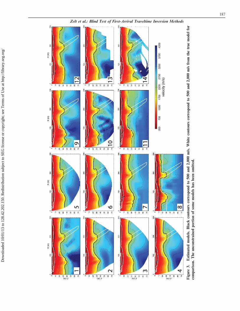
3.

Est

ima

ted

mo

del

s.B

lack

con

tou

rsco

rres

po

nd

to5

00

an

d2

,00

0m

/s.

Wh

ite

con

tou

rsco

rres

po

nd

to5

00

an

d2

,00

0m

/sfr

om

the

tru

em

od

elfo

r

com

pa

riso

n.

Th

eu

nco

nst

rain

edp

ort

ion

of

som

em

od

els

ha

sb

een

om

itte

d.

187


Dow

nloa

ded

10/0

1/13

to 1

28.4

2.20

2.15

0. R

edis

trib

utio

n su

bjec

t to

SEG

lice

nse

or c

opyr

ight

; see

Ter

ms

of U

se a

t http

://lib

rary

.seg

.org

/

1-D initial model is then iteratively refined with 2-D

WET inversion (Schuster and Quintus-Bosz, 1993). For

Model 3, a smooth Rayfract inversion was run with

default parameters and 999 WET iterations. For Model

4, all velocities higher than 3,000 m/s were reset to

3,000 m/s in the initial Delta-t-V 1-D model, and WET

was rerun using this modified starting model. The final

models were obtained after the same number of WET

iterations, using both the default and modified Delta-t-V

initial models.

The two WET tomograms are very similar, despite

the missing higher velocities in the modified Delta-t-V

initial model. Also, these tomograms show minimum

correlation with horizontal layering artifacts of the 1-D

initial model, and agree with a wavefront refraction

interpretation in which the first breaks were mapped

interactively to assumed refractors and the layer-based

wavefront refraction method of Ali Ak (1990) applied.

Models 5 and 6

These models were also generated using RayfractHsoftware that uses the WET tomography approach.

Default parameter values were used with the following

exceptions: the iteration count was increased to 200

and the wavepath width (percent of one period) was

decreased to 4 percent. The effect of smoothing the

noisy first arrival times and using a 1-D versus 2-D

starting velocity model were investigated.

To obtain both final models the traveltimes were

smoothed with a polynomial filter of degree two and a

window size of 127 samples. The RMS difference for the

filtered and raw times was 0.048ms. Model 5 used a 1-D

initial velocity model and Model 6 used the 2-D Delta-t-

V initial model. These two models were compared with

the models obtained using the same parameters and

unfiltered (unsmoothed) traveltimes; the comparison

reveals only small velocity differences in both cases,

typically 10–20 m/s. The difference between the final

models from the 1-D and 2-D starting models are only

significant near the model edges, but are on the order of

5% or less elsewhere.

Models 7 and 8

These models were created using the SeisImager/2-

D software available from Geometrics. The intent was

to show an example of model non-uniqueness associated

with the initial model by using two different starting

velocity models. For Model 7, the starting model was a

simple 1-D velocity model in which velocity increases

with depth. For Model 8, the starting model was a 2-D

two-layer velocity model obtained through the delay

time method; the velocities of the second layer were

Table 1. Algorithms, fits and statistical comparisons with the true model for each estimated model.

Model Algorithm Reference TRMS (ms)

Difference Relative difference

Mean1 (m/s) Std. dev. (m/s) Mean1 (%) Std. dev. (%)

1 GeoTomo Zhang and

Toksoz (1998)

1.3 2237 564 29.3 24.0

2 Rayfract rayfract.com 1.08 2208 466 23.2 23.4





7 Geometrics SeisImager/2-D geometrics.com2 1.11 2223 479 23.0 24.8

8 Geometrics SeisImager/2-D geometrics.com2 1.40 216 524 +7.1 37.9

9 Geogiga DW Tomo geogiga.com3 1.72 2166 522 21.5 26.4

10 Geogiga DW Tomo geogiga.com3 1.13 2111 469 20.6 22.1

11 DLT (Deformable layer

tomography)

Zhou (2006) 1.05 2141 449 21.2 24.6

12 Phase Inversion Ellefsen (2009) 1.2 2152 439 21.3 22.2

13 WARRP Ditmar et al.

(2009)

1.32 2173 571 21.4 26.3

14 Tomog Preston et al.

(2007)

1.59 293 675 +0.4 27.7

1vestimated -vtrue2http://www.geometrics.com/geometrics-products/seismographs/download-seismograph-software3http://geogiga.com/en/dwtomo.php

188


Dow

nloa

ded

10/0

1/13

to 1

28.4

2.20

2.15

0. R

edis

trib

utio

n su

bjec

t to

SEG

lice

nse

or c

opyr

ight

; see

Ter

ms

of U

se a

t http

://lib

rary

.seg

.org

/

manually determined from plots of the data using a

reducing velocity. Although the two final models show

some significant differences, their large-scale features

are similar.

Model 9

This model was created using the software DW

Tomo 6.0 developed by Geogiga Technology Corp. This

method employs a gridded model, the graph method

(also known as the shortest path method) to calculate

traveltimes and raypaths, and a smoothing-regularized

inverse approach to iteratively update the model. A

velocity gradient model was used as the starting model

with the surface velocity set to 400 m/s, the bottom

velocity set to 5,000 m/s, and the maximum depth set to

100 m. The model’s horizontal and vertical grid spacing is

1.5 m and 1.0 m. The smoothing lengths are 7.5 m 3 5 m.

The final model was obtained from the 10th iteration.

Model 10

This model was also created using the DW Tomo

6.0 software. For the model parameterization, a horizon-

tal and vertical node spacing of 1 meter was used. The

default smoothing parameters of 15 m horizontally and

3.75 m vertically resulted in a smooth model with an

RMS misfit of 1.91 ms. This is the model that would most

likely have been chosen to submit to a client if this was

real field data. However, to explore the range of models

between those with very little detail and few artifacts and

those with a high level of detail, but also some artifacts,

the smoothing was decreased to 6 m horizontally and

2.5 m vertically. The resulting final model has more detail

and an RMS misfit of 1.13 ms, but it contains some

inversion artifacts. However, the bedrock surface is

imaged better using the lower smoothing parameters,

suggesting that the lower smoothing could aid in

interpretation, as long as the artifacts are recognized as

such and not included in the interpretation.

Model 11

This model was created using the deformable layer

tomography (DLT) method of Zhou (2006). The DLT

method parameterizes the model with a number of

thickness-varying layers, and each layer’s velocity

function can be constant, a gradient, or laterally

varying. The method is able to invert for either the

layer geometry, or layer velocity functions, or both

simultaneously. A multi-scale scheme is employed to

regularize the inversion for layer geometry and velocity

functions. There is no smoothing of the model during or

after the inversion process. However, prior information

was incorporated in the form of a no-low-velocity-zone

assumption such that the velocity is forced to increase

with depth at each X position.

The DLT method was carried out in three steps.

First, a long-wavelength model was built by inverting

for the layer geometry of 12 constant-velocity layers;

this 12-layer model reduced the RMS misfit to 1.99 ms.

Second, the model was divided into 34 layers and the

inversion for layer geometry resulted in an RMS misfit

of 1.17 ms. Finally, both the layer geometries and

velocities were inverted for, yielding an RMS misfit of

1.05 ms. The non-low-velocity-zone assumption ensured

a stable solution, although it precluded the ability to

resolve low-velocity zones.

Model 12

This model was created using a wave-based, phase-

inversion method that is the frequency-domain equivalent

of traveltime inversion initially developed by Min and

Shin (2006) for large-scale seismic studies. The observed

traveltimes are transformed to their frequency-domain

equivalents, which are the observed phases. The calcu-

lated phases are obtained from the solution of the scalar

Helmholtz equation. The model is updated using a

backpropagation method that is based on Rytov wave-

paths. Ellefsen (2009) modified the phase inversion method

for application to near-surface data, including the param-

eterization of the model, corrections to the observed

phases, and selection of an appropriate complex frequency.

The model for the modified inversion is isotropic and it is

parameterized using the natural logarithm of the slowness.

A smooth starting model was generated using a

separate time-domain method that provided an RMS

misfit of less than 10 ms. For the phase inversion, a

complex frequency of 20+i80 Hz was chosen that

satisfies the criterion in Ellefsen (2009). Because the

current implementation of phase inversion requires

significant computer memory, only the traveltimes from

every fourth shot were used, for a total of 26 shots,

yielding a final RMS misfit of 1.2 ms. A forward

calculation of all 101 shots using the final model also

yields an RMS misfit of 1.2 ms, implying that the model

structure estimated using 26 shots is sufficient to fit the

data from all 101 shots.

Model 13

This model was created using the WARRP (Wide

Aperture Reflection/Refraction Profiling) algorithm

(Ditmar et al., 1999). Both interface geometries and

the velocity distribution in layers are determined. The

intensity of model smoothing is applied as a frac-

tional change of velocities determined by the user. The

inversion was done sequentially layer by layer, to a total

of four layers, by first inverting to obtain a velocity

profile and then establishing the position of the next

interface by gather analyses. The model grid spacing was

10.2 m vertically and horizontally. Finally, ray density

189


Dow

nloa

ded

10/0

1/13

to 1

28.4

2.20

2.15

0. R

edis

trib

utio

n su

bjec

t to

SEG

lice

nse

or c

opyr

ight

; see

Ter

ms

of U

se a

t http

://lib

rary

.seg

.org

/

distribution analysis was used to exclude parts of the

model with little ray coverage.

Model 14

This model was created using the tomographic

program of Preston et al. (2007) in which an iterative

inverse procedure is used to find incremental changes inmodel parameters to optimally fit travel-time residuals

(observed minus calculated), subject to velocity struc-

ture smoothing constraints using a Laplacian operator

that can accommodate different degrees of smoothing in

the vertical and horizontal directions. Ray paths are

calculated by following the finite-difference (eikonal)

traveltime gradient from a receiver to the source. Model

slowness perturbations are solved for by a conjugate-gradient least-squares approach.

A rough initial velocity model (two layers over a

half space) was developed using an average of all shot

records. Model grid node spacing is 1 m. Model

roughness, initially set low (very smooth), was allowed

to increase with successive iterations until the traveltime

residuals did not decrease sufficiently relative to model

roughness increases.

Results

Figures 4 and 5 show horizontal and vertical

profiles, respectfully, from the 14 estimated models, as

well as the true model and the average of the estimated

models. These profiles, along with Figs. 1(c-d), show

that the variation between the models generally increas-

es with depth. This illustrates the greater level of model

uncertainty and non-uniqueness in the deeper parts ofmodels derived from refraction data using first-arrival

times caused by the decreasing number of rays and

range of ray angles sampling the model as depth

Figure 4. Comparison of horizontal slices through the true model (thick gray line), average estimated model (thick

dashed line) and each estimated model at Z = 5, 25 and 40 m.

190


Dow

nloa

ded

10/0

1/13

to 1

28.4

2.20

2.15

0. R

edis

trib

utio

n su

bjec

t to

SEG

lice

nse

or c

opyr

ight

; see

Ter

ms

of U

se a

t http

://lib

rary

.seg

.org

/

increases. The majority of the constrained model region

has a variation among the estimated models with a

standard deviation of less than 200 m/s (Fig. 1(c)) or less

than 10% (Fig. 1(d)). Other than near the edges of the

constrained model region, the location with the greatest

variation among the estimated models is at the top ofthe basement between lateral positions 90 and 170 m,

i.e., between the basement offset and the dipping fault

zone (Figs. 4 and 5). This may be because most of the

modeling approaches seek a smooth model and have

performed differently in how they handle this segment

of the basement that is a sharp feature in the true model,

both vertically and horizontally.

The RMS misfit between the true and predicteddata for the 14 models varies from 1.05 to 1.72 ms

(Table 1). One would expect that the models with the

Figure 5. Comparison of vertical slices through the true model (thick gray line), average estimated model (thick dashed

line) and each estimated model at X = 65, 135, 185 and 235 m.

191


Dow

nloa

ded

10/0

1/13

to 1

28.4

2.20

2.15

0. R

edis

trib

utio

n su

bjec

t to

SEG

lice

nse

or c

opyr

ight

; see

Ter

ms

of U

se a

t http

://lib

rary

.seg

.org

/

lowest RMS misfits (models 11, 2 and 7) would contain

the most structure and that the models with the highest

RMS misfits (models 9, 14 and 8) would contain the

least amount of structure. However, this trend is not

observed, suggesting that the amount of structure in the

estimated models is controlled by the particular

algorithm used and assumptions made, rather than the

fit between the true and predicted data. The mean of the

difference between the estimated and true velocities

shows that the estimated models are biased toward low

velocities, averaging 160 m/s lower than the true velocity

(Table 1). The standard deviation of the difference

between the estimated and true velocities is quite

consistent and surprisingly high, averaging ,500 m/s.

The mean of the relative difference between the

estimated and true velocities is generally quite small,

averaging ,1.7%. Also, the standard deviation of the

relative difference between the estimated and true

velocities is quite consistent, averaging ,25%. The

reason the mean is large by comparison to the relative

mean is that the velocities in the model vary by a factor

of about 15, and the mean is dominated by the

differences in the high velocity regions. Overall, the

two measures of velocity difference are surprisingly

similar for all the estimated models, despite the fact that

the models are quite different (Fig. 3), suggesting these

differences are dependent on the model and the data,

not the algorithm used or assumptions made.

The average estimated model includes a smooth

approximation of the large-scale structure of the true

model (Fig. 1), although the shallow low-velocity zone

at ,5-m depth between X 5 12.5 and 125 m is absent in

the average estimated model, and in all of the individual

estimated models (Fig. 5). This confirms the long-

identified inability of conventional first-arrival-time

methods to image a low-velocity zone unless it is large

in size and/or magnitude. The offset in the bedrock

centered at X 5 95 m is smoothly represented in the

average model, and all of the estimated models, as is the

top of the dipping low-velocity fault zone centered at X

5 185 m. The expression of the dipping fault zone is

consistent, albeit very smooth, in the estimated models,

reflected in the low relative standard deviation of the

models of ,5% at the fault location (Fig. 1(d)). The

fault zone anomaly fades away near the base of ray

coverage at about 50-m depth in the average model. The

average estimated model, and the majority of the

individual estimated models, overestimate the basement

velocity below ,40-m depth on the left side of the

model. Exceptions to this are models 2, 5, 7, 8, 11 and

12. This is likely because of the reduced lateral

resolution caused by predominantly sub-horizontal ray

coverage at this depth (Fig. 2), and/or an overestimation

of velocity in the starting models at this depth, and/or a

velocity-depth tradeoff related to the failure to image

the shallow low-velocity zone, the offset in the basement

at X 5 95 m, and the dipping low-velocity zone on the

right side of the basement. A comparison between the

white and black 2,000 m/s velocity contours in Fig. 3, a

rough proxy for the bedrock contact in this case, shows

that most of the estimated models predict this contour

to be deeper than the true contour; exceptions are

models 8, 10 and 11. This is likely because of the way in

which a sharp boundary is represented in a smooth

tomographic model.

Discussion and Conclusions

The model(s) derived using any particular algo-

rithm in this paper cannot be expected to fully represent

all the advantages and disadvantages of that algorithm.

The final models are as much a consequence of the

subjective modeling choices made by a particular author

as they are a function of the software used. Therefore,

the main contribution of this paper is in providing a

sense of the range of models that can result from

different people using different algorithms analyzing the

same set of first-arrival traveltime data, as opposed to a

determination of the best or worst algorithm.

Overall, the 14 models are consistent in terms of

their large-scale features (Fig. 3) and they show the

large-scale features of the true model, making the case

that refraction inversion and tomography is robust. This

is especially significant when considering that the

eight algorithms used vary significantly in their model

parameterization (i.e., fine grid versus layered), forward

and inverse modeling approaches, and prior information

(i.e., amount of model smoothing or lack there of).

However, model differences only reflect the algorithms

used and assumptions made, they do not reflect

differences in first-arrival picking, which would occur

with different people picking the same set of real data.

All methods used in this paper, except the multi-

scale approach of the DLT method (model 11), use some

form of model smoothing constraint to seek a smooth

model. This is a common methodological aspect of

seismic tomography and it is intended to deal with

model non-uniqueness and to keep the model smooth in

accordance with the assumptions of ray theory. It is also

used to honor Occam’s principle, which states that the

simplest, i.e., minimum-structure, solution is the best

(Constable et al., 1987). However, enforcing model

smoothness must be considered when interpreting a final

model and assessing its geological reasonableness. For

example, if a relatively sharp boundary is believed to

exist, then its position and shape in a smooth model will

be indicated by the velocity contour that corresponds to

a value that is roughly midway between the velocities

192


Dow

nloa

ded

10/0

1/13

to 1

28.4

2.20

2.15

0. R

edis

trib

utio

n su

bjec

t to

SEG

lice

nse

or c

opyr

ight

; see

Ter

ms

of U

se a

t http

://lib

rary

.seg

.org

/

above and below the actual boundary (Zelt et al., 2003).

In the case of the 14 estimated models in this paper,

all of them are smooth, but all of them contain an

expression of two of the most prominent features in

the true model, that is, the bedrock offset centered at

X 5 95 m, and the dipping low-velocity fault zone

starting at X 5 185 m at 20-m depth. Furthermore, if

these models were derived from real data, and if there

were some prior knowledge of the study area

suggesting that either of these features might be

present somewhere in the subsurface, an interpretation

of any of these models would accurately locate the

lateral position of these two features. On the other

hand, the depth of the bedrock surface is typically

overestimated by a few meters (,10% of the depth)

using the 2,000 m/s contour as a proxy in the smooth

models. Also, none of the estimated models contain an

expression of the shallow low-velocity zone on the left

side in the true model, presumably because it is

relatively small in size and weak in magnitude (no

more than ,200 m/s).

The type of survey needed to acquire the true

data–101 shots recorded by a static array of 100

geophones–is realistic for modern refraction surveys

(e.g., Powers et al., 2007). The results of using the phase

inversion method to derive model 12 suggest that as few

as 26 shots could yield a sufficiently accurate model in

terms of the large-scale features. This shows that the

time, equipment and human resources needed to carry

out a successful 2-D refraction survey are relatively

modest compared to a typical seismic reflection survey.

In addition, the seismograms from a refraction survey

can be exploited further than just using the first-arrival

times. For example, some modeling algorithms allow

later refracted and reflected arrivals to be used to

provide additional model constraint, in particular, on

the geometry of layer boundaries, such as the bedrock

surface in this study. Finally, refraction data can be

amenable to conventional multi-channel reflection

processing to yield a low-fold stack, as well as 2-D full

waveform inversion (e.g., Gao et al., 2007; Smithyman

et al., 2009).

Acknowledgements

Karl J. Ellefsen (U.S. Geological Survey) and Leiph A.

Preston (Sandia National Laboratories) helped to develop

models 12 and 14, respectively. The review of the manuscript

by Karl J. Ellefsen is gratefully acknowledged. CZ acknowl-

edges support from DOE grant DE-FG02-03ER63662. Sandia

National Laboratories is a multi-program laboratory operated

by Sandia Corporation, a wholly owned subsidiary of Lock-

heed Martin company, for the U.S. Department of Energy’s

National Nuclear Security Administration under contract DE-

AC04-94AL85000. References to any specific commercial

product, process, or service by trade name, trademark,

manufacturer, or otherwise does not constitute or imply its

endorsement, recommendation, or favoring by the United

States Government or any agency thereof.

References

Ali Ak, M., 1990, An analytical raypath approach to the

refraction wavefront method: Geophysical Prospecting,

38, 971–982.

Asten, M.W., Stephenson, W.R., and Davenport, P.N., 2005,

Shear-wave velocity profile for Holocene sediments

measured from microtremor array studies, SCPT, and

seismic refraction: Journal of Environmental and

Engineering Geophysics, 10, 235–242.

Constable, S.C., Parker, R.L., and Constable, C.G., 1987,

Occam’s inversion: a practical algorithm for generating

smooth models from electromagnetic sounding data:

Geophysics, 52, 289–300.

Deen, T., and Gohl, K., 2002, 3-D tomographic seismic

inversion of a paleochannel system in central New South

Wales, Australia: Geophysics, 67(5) 1364–1371.

Ditmar, P., Penopp, J., Kasig, R., and Makris, J., 1999,

Interpretation of shallow refraction seismic data by

reflection/refraction tomography: Geophysical Pro-

specting, 47, 871–901.

Ellefsen, K.J., 2009, A comparison of phase inversion and

traveltime tomography for processing near-surface re-

fraction traveltimes: Geophysics, 74(6) WCB11–WCB24.

Gabriels, P., Snieder, R., and Nolet, G., 1987, In situ

measurements of shear-wave velocity in sediments with

higher-mode Rayleigh waves: Geophysical Prospecting,

35, 187–196.

Gao, F., Levander, A., Pratt, R.G., Zelt, C.A., and Fradelizio,

G.-L., 2007, Waveform tomography at a ground water

contamination site: Surface reflection data: Geophysics,

72, G45–G55.

Gebrande, H., and Miller, H., 1985, Refraktionsseismik (in

German) in Angewandte Geowissenschaften II, Bender,

F. (ed.), Ferdinand Enke, Stuttgart, 226–260.

Gibson, B.S., Odegard, M.E., and Sutton, G.H., 1979,

Nonlinear least-squares inversion of traveltime data

for a linear velocity-depth relationship: Geophysics, 44,

185–194.

Lomax, A., 1994, The wavelength-smoothing method for

approximating broad-band wave propagation through

complicated velocity structures: Geophysical Journal

International, 117, 313–334.

Martı, D., Carbonell, R., Flecha, I., Palomeras, I., Font-Capo,

J., Vazquez-Sune, E., and Perez-Estaun, A., 2008, High-

resolution seismic characterization in an urban area:

Subway tunnel construction in Barcelona, Spain:

Geophysics, 73(2) B41–B50.

Min, D.J., and Shin, C., 2006, Refraction tomography using a

waveform-inversion back-propagation technique: Geo-

physics, 71(3) R21–R30.

Moro, G.D., Pipan, M., and Gabrielli, P., 2007, Rayleigh wave

dispersion curve inversion via genetic algorithms and

193


Dow

nloa

ded

10/0

1/13

to 1

28.4

2.20

2.15

0. R

edis

trib

utio

n su

bjec

t to

SEG

lice

nse

or c

opyr

ight

; see

Ter

ms

of U

se a

t http

://lib

rary

.seg

.org

/

marginal posterior probability density estimation: Jour-

nal of Applied Geophysics, 61, 39–55.

Palmer, D., 1980. The generalized reciprocal method of seismic

refraction interpretation, Society of Exploration Geo-

physics, Tulsa, OK, 104 pp.

Park, C.B., Miller, R.D., and Xia, J., 1999, Multi-channel

analysis of surface waves: Geophysics, 64, 800–808.

Pelton, J.R., 2005, Near-surface seismology: Surface-based

methods in Near-Surface Geophysics, Butler, D. (ed.),

Society of Exploration Geophysics, Tulsa, OK, 219–263.

Powers, M.H., Haines, S., and Burton, B.L., 2007, Compres-

sional and shear wave seismic refraction tomography at

Success Dam, Porterville, California: in Proceedings of

the Symposium on the Application of Geophysics to

Engineering and Environmental Problems, 20, 31–40.

Preston, L., Smith, K., and von Seggern, D., 2007, P wave

velocity structure in the Yucca Mountain, Nevada

region: Journal of Geophysical Research, 112, B11305,

doi: 10.1029/2007JB005005.

Schuster, G.T., and Quintus-Bosz, A., 1993, Wavepath eikonal

traveltime inversion-Theory: Geophysics, 58(9) 1314–

1323.

Sheehan, J.R., Doll, W.E., and Mandell, W., 2005, An

evaluation of methods and available software for seismic

refraction tomography analysis: Journal of Environ-

mental and Engineering Geophysics, 10(1) 21–34.

Smithyman, B., Pratt, R.G., Hayles, J., and Wittebolle, R.,

2009, Detecting near-surface objects with seismic wave-

form tomography: Geophysics, 74, WCC119–WCC127.

Yordkayhun, S., Tryggvason, A., Norden, B., Juhlin, C., and

Bergman, B., 2009, 3D seismic traveltime tomography

imaging of the shallow subsurface at the CO2SINK project

site, Ketzin, Germany: Geophysics, 74(1) G1–G15.

Zelt, C.A., Azaria, A., and Levander, A., 2006, 3D seismic

refraction traveltime tomography at a groundwater

contamination site: Geophysics, 71(5) H67–H78.

Zelt, C.A., Liu, H., and Chen, J., 2011. Frequency-dependent

traveltime tomography for near-surface seismic data:

Sensitivity kernels and synthetic and real data examples,

Abstract NS41A-05, Fall Meeting, AGU, San Fran-

cisco, CA.

Zelt, C.A., Sain, K., Naumenko, J.V., and Sawyer, D.S., 2003,

Assessment of crustal velocity models using seismic

refraction and reflection tomography: Geophysical

Journal International, 153, 609–626.

Zelt, C.A., and Smith, R.B., 1992, Seismic traveltime inversion

for 2-D crustal velocity structure: Geophysical Journal

International, 108, 16–34.

Zhang, J., and Toksoz M, N., 1998, Nonlinear refraction

traveltime tomography: Geophysics, 63, 1726–1737.

Zhou, H., 2006, Multiscale deformable-layer tomography:

Geophysics, 71, R11–R19.

194


Dow

nloa

ded

10/0

1/13

to 1

28.4

2.20

2.15

0. R

edis

trib

utio

n su

bjec

t to

SEG

lice

nse

or c

opyr

ight

; see

Ter

ms

of U

se a

t http

://lib

rary

.seg

.org

/

blind test of methods for obtaining 2-d near-surface seismic

Documents