International Journal of Bioelectromagnetism www/ijbem.org Vol. 6, No. 1, pp. xx - xx, 2004

Blind Signal Processing Methods for Analyzing Multichannel Brain Signals

Andrzej Cichocki Laboratory for Adavnced Brain Signal Processing, RIKEN, Brain Science Japan

Correspondence: Dr. A. Cichocki , Laboratory for Advanced Brain Signal Processing, Brain Science Institute, Riken 2-1 Hirosawa, Wako-shi, Saitama 351-0198, E-mail: cia@brain.riken.jp , Tel. +81 (0)48 467 9668, Fax. +81 (0)48 467 9686

JAPAN Abstract. A great challenge in neurophysiology is to asses non-invasively the physiological changes occurring in different parts of the brain. These activation can be modeled and measured often as neuronal brain source signals that indicate the function or malfunction of various physiological sub-systems. To extract the relevant information for diagnosis and therapy, expert knowledge is required not only in medicine and neuroscience but also statistical signal processing. Besides classical signal analysis tools (such as adaptive supervised filtering, parametric or non-parametric spectral estimation, time-frequency analysis, and higher-order statistics), new and emerging blind signal processing (BSP) methods, especially, generalized component analysis (GCA) including fusion (integration) of independent component analysis (ICA), sparse component analysis (SCA), time-frequency component analyzer (TFCA) and nonnegative matrix factorization (NMF) can be used for analyzing brain data, especially for noise reduction and artefacts elimination, enhancement, detection and estimation of neuronal brain source signals. The recent trends in the BSP is to consider problems in the framework of matrix factorization or more general signals decomposition with probabilistic generative and tree structured graphical models and exploit a priori knowledge about true nature and structure of latent (hidden) variables or brain sources such as spatio-temporal decorrelation, statistical independence, sparseness, smoothness or lowest complexity in the sense e.g., of best linear predictability. The goal of BSP can be considered as estimation of sources and parameters of a mixing system or more generally as finding a new reduced or hierarchical and structured representation for the observed brain data that can be interpreted as physically meaningful coding or blind source estimation. The key issue is to find such transformation or coding (linear or nonlinear) which has true neurophysiological and neuroanatomical meaning and interpretation. In this paper, we briefly discuss how some novel blind signal processing techniques such as blind source separation, blind source extraction and various blind source separation and signal decomposition methods can be applied for analysis and processing EEG data. We discuss also a promising application of BSP to early detection of Alzheimer disease (AD) using only EEG recordings. Keywords: Blind Source Separation (BSS), Independent Component Analysis (ICA), Sparse Compoent , Analysis (SCA), Nonnegative Matrix Factorization (NMF), Time Frequency Component Analyzer.

1. Introduction The nervous systems of humans and animals must encode and process sensory information within the context of noise and interference, and the signals which are encode (the images, sounds, smell, odors, etc.) have very specific statistical properties. One of the challenging tasks is how to detect, enhance and localize and classify superimposed and overlapping, multidimensional brain source signals corrupted by noise and other interferences. To understand human neurophysiology, we currently rely on several types of non-invasive neuroimaging techniques. These techniques include electroencephalography (EEG) and magnetoencephalography (MEG). In recent years, an increasing interest has been observed in applying high density array EEG/MEG systems with more than one hundreds channels to analyze patterns and imaging of the human brain, where EEG/MEG have desirable property of excellent time resolution [Babiloni et al., 2004, Makeig et al., 2004, Malmivuo and Plonsey, 1995]. This property combined with other systems such as eye tracking,

ECG (electrocardiography) and EMG (electromyography) systems with relatively low cost of instrumentations makes it attractive for investigating the some higher cognitive mechanisms in the brain or mental states (such as emotion, stress, attention, fatigue) and opens a unique window to investigate the dynamics of human brain functions as they are able to follow changes in neural activity on a millisecond time-scale. In comparison, the other functional imaging modalities positron emission tomography (PET) and functional magnetic resonance imaging (fMRI) are limited in temporal resolution to time scales on the order of, at best, one second by physiological and signal-to-noise considerations. Determining active regions of the brain, given EEG/MEG measurements on the scalp is an important problem. A more accurate and reliable solution to such a problem can give information about higher brain functions and patient-specific cortical activity. However, estimating the location and distribution of electric current sources within the brain from EEG/MEG recording is an ill-posed problem, since there is no unique solution and the solution does not depend continuously on the data. The ill-posedness of the problem and distortion of sensor signals by large noise sources makes finding a correct solution a challenging analytic and computational problem [Babiloni et al., 2004, Cichocki and Amari, 2003].

1.1. Why Blind Sources Separation and Signal Decomposition ? In order to understand the higher order functioning of the brain, it is necessary to develop new

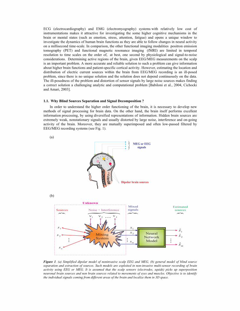
methods of signal processing for brain data. On the other hand, the brain itself performs excellent information processing, by using diversified representations of information. Hidden brain sources are extremely weak, nonstationary signals and usually distorted by large noise, interference and on-going activity of the brain. Moreover, they are mutually superimposed and often low-passed filtered by EEG/MEG recording systems (see Fig. 1).

(a)

Dipolar brain sources

} MEG or EEGsignals

(b)

NeuralNetworkModel

MixingSystem

1s

2s

1� k�2�

1x

2x 1s

ms

2s

{ { {

Estimatedsources{Mixed

signalsNoise + InterferenceSources

Unknown

mx

ns

Figure 1. (a) Simplified dipolar model of noninvasive scalp EEG and MEG, (b) general model of blind source separation and extraction of sources. Such models are exploited in non-invasive multi-sensor recording of brain activity using EEG or MEG. It is assumed that the scalp sensors (electrodes, squids) picks up superposition neuronal brain sources and non brain sources related to movements of eyes and muscles. Objective is to identify the individual signals coming from different areas of the brain and localize them in 3D space.

2. Simple Linear Models

The mixing and filtering processes of the unknown input sources may have different mathematical or physical models, depending on the specific applications [Hyvarinen et al., 2001; Amari and Cichocki, 1998]. Most of linear BSS models in the simplest forms can be expressed algebraically as some specific problems of matrix factorization: Given observation (often called sensor or data) matrix X perform the matrix factorization:

X = H S + V (1)

where:

X = [ x(1), x(2), ..., x(N)] -- available sensor signals, S = [ s(1), s(2), ..., s(N) ] -- unknown source signals,

V = [ v(1), v(2), ..., v(N) ] -- unknown noise,

V is matrix representing the additive noise (see Table 1).

(a)

H W�)( ks )(ky)(kx

m nn

Unknown

v( )k

(b)

Unknownprimarysources

Unknownmatrix

Observablemixedsignals

Neural network

Separatedoutputsignals

�+

+

�+

+

+

�

+

�+

+

s k( ) x k( )

x k( )

y k( )

y k( )

( )k

( )k

s k( )

LearningAlgorithm

111 111 1

1

n m

m

mn

1n

m1

1m

n1

nmn

h

h

h

h

w

w

w

w

v

v

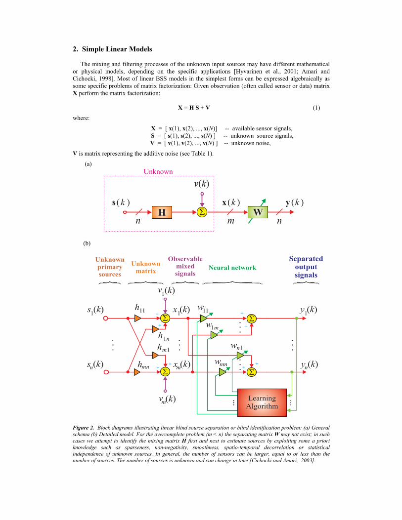
Figure 2. Block diagrams illustrating linear blind source separation or blind identification problem: (a) General schema (b) Detailed model. For the overcomplete problem (m < n) the separating matrix W may not exist; in such cases we attempt to identify the mixing matrix H first and next to estimate sources by exploiting some a priori knowledge such as sparseness, non-negativity, smoothness, spatio-temporal decorrelation or statistical independence of unknown sources. In general, the number of sensors can be larger, equal to or less than the number of sources. The number of sources is unknown and can change in time [Cichocki and Amari, 2003].

Alternatively, the process can be described in on-line form as (see Fig. 2)

x(k) = H s(k) + v(k), k = 1, 2, ..., N (2)

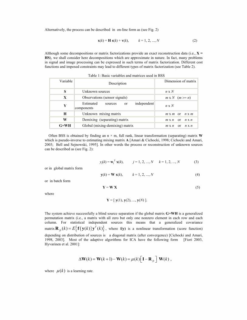
Although some decompositions or matrix factorizations provide an exact reconstruction data (i.e., X = HS), we shall consider here decompositions which are approximate in nature. In fact, many problems in signal and image processing can be expressed in such terms of matrix factorization. Different cost functions and imposed constraints may lead to different types of matrix factorization (see Table 2).

Table 1: Basic variables and matrices used in BSS

Variable Description Dimension of matrix

S Unknown sources n x N X Observations (sensor signals) m x N (m >= n)

Y Estimated sources or independent components n x N

H Unknown mixing matrix m x m or n x m W Demixing (separating) matrix m x n or n x n

G=WH Global (mixing-demixing) matrix m x n or n x n Often BSS is obtained by finding an n × m, full rank, linear transformation (separating) matrix W which is pseudo-inverse to estimating mixing matrix A [Amari & Cichocki, 1998; Cichocki and Amari, 2003; Bell and Sejnowski, 1995]. In other words the process or reconstruction of unknown sources can be described as (see Fig. 2):

yj(k) = wjT x(k), j = 1, 2, ..., N k = 1, 2, ..., N (3)

or in global matrix form

y(k) = W x(k), k = 1, 2, ..., N (4)

or in batch form

Y = W X (5)

where

Y = [ y(1), y(2), ..., y(N) ].

The system achieve successfully a blind source separation if the global matrix G=WH is a generalized permutation matrix (i.e., a matrix with all zero but only one nonzero element in each row and each column. For statistical independent sources this means that a generalized covariance matrix ( ){ }( ) ( ) ( )T

fy k E k k=R f y y , where f(y) is a nonlinear transformation (score function)

depending on distribution of sources is a diagonal matrix (after convergence) [Cichocki and Amari, 1998, 2003]. Most of the adaptive algorithms for ICA have the following form [Fiori 2003, Hyvarinen et al. 2001]:

( ) ( 1) ( ) ( ) ( ) ,fyk k k k kµ ∆ = + − = − W W W I R W

where ( )kµ is a learning rate.

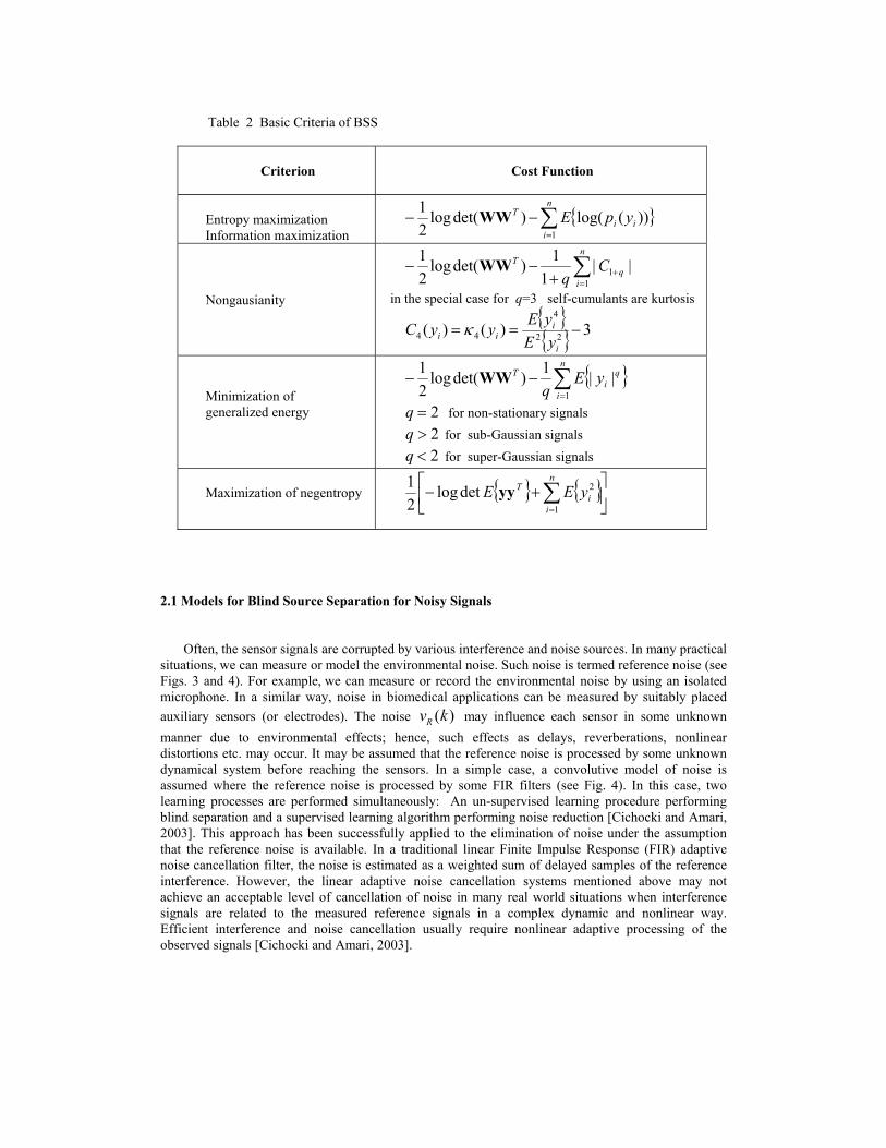
Table 2 Basic Criteria of BSS

Criterion

Cost Function

Entropy maximization Information maximization

{ }∑=

−−n

iii

T ypE1

))(log()det(log21 WW

Nongausianity

∑=

++−−

n

iq

T Cq 1

1 ||1

1)det(log21 WW

in the special case for q=3 self-cumulants are kurtosis { }{ } 3)()( 22

4

44 −==i

iii yE

yEyyC κ

Minimization of generalized energy

{ }∑=

−−n

i

qi

T yEq 1

||1)det(log21 WW

2=q for non-stationary signals 2>q for sub-Gaussian signals 2<q for super-Gaussian signals

Maximization of negentropy { } { }

+− ∑

=

n

ii

T yEE1

2detlog21 yy

2.1 Models for Blind Source Separation for Noisy Signals

Often, the sensor signals are corrupted by various interference and noise sources. In many practical situations, we can measure or model the environmental noise. Such noise is termed reference noise (see Figs. 3 and 4). For example, we can measure or record the environmental noise by using an isolated microphone. In a similar way, noise in biomedical applications can be measured by suitably placed auxiliary sensors (or electrodes). The noise ( )Rv k may influence each sensor in some unknown manner due to environmental effects; hence, such effects as delays, reverberations, nonlinear distortions etc. may occur. It may be assumed that the reference noise is processed by some unknown dynamical system before reaching the sensors. In a simple case, a convolutive model of noise is assumed where the reference noise is processed by some FIR filters (see Fig. 4). In this case, two learning processes are performed simultaneously: An un-supervised learning procedure performing blind separation and a supervised learning algorithm performing noise reduction [Cichocki and Amari, 2003]. This approach has been successfully applied to the elimination of noise under the assumption that the reference noise is available. In a traditional linear Finite Impulse Response (FIR) adaptive noise cancellation filter, the noise is estimated as a weighted sum of delayed samples of the reference interference. However, the linear adaptive noise cancellation systems mentioned above may not achieve an acceptable level of cancellation of noise in many real world situations when interference signals are related to the measured reference signals in a complex dynamic and nonlinear way. Efficient interference and noise cancellation usually require nonlinear adaptive processing of the observed signals [Cichocki and Amari, 2003].

+

_�

(Nonlinear)Adaptive

Filter

LearningAlghorithm

s( )k

Desiredsignal

PrimarySensor

Primarysignal

d( ) = s( ) + ( )k k k�

e( ) = s( )k k

^

^

Referencenoise or signal

Referencesensor

�( ) - Interferencek

�R( )k

�( )k

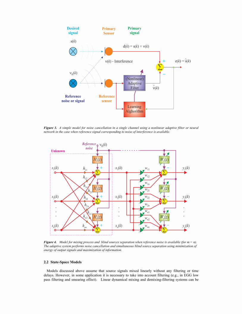
Figure 3. A simple model for noise cancellation in a single channel using a nonlinear adaptive filter or neural network in the case when reference signal corresponding to noise of interference is available.

+

+

+

_

_

_

H z1( )

H z2( )

H zn( )

W z1( )

W z2( )

W zn( )

s k1( ) x k1( ) y k1( )

s k2( ) x k2( ) y k2( )

s kn( ) x kn( ) y kn( )

Referencenoise

Unknown

�R( )k

11h

12h

nh1

21h

22h

nh2

1nh

2nh

nnh

w11

w12

w1n

w21

w22

w2n

wn1

wn2

wnn

Figure 4. Model for mixing process and blind sources separation when reference noise is available (for m = n). The adaptive system performs noise cancellation and simultaneous blind source separation using minimization of energy of output signals and maximization of information. 2.2 State-Space Models Models discussed above assume that source signals mixed linearly without any filtering or time delays. However, in some application it is necessary to take into account filtering (e.g., in EGG low pass filtering and smearing effect). Linear dynamical mixing and demixing-filtering systems can be

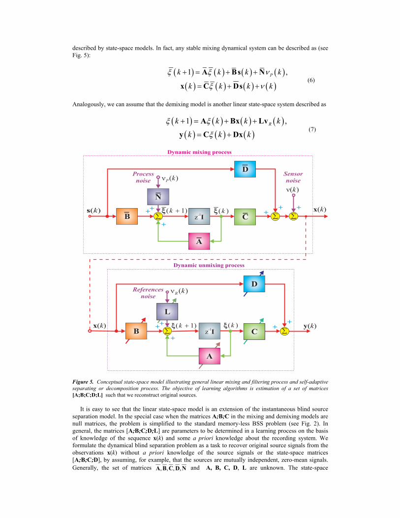
described by state-space models. In fact, any stable mixing dynamical system can be described as (see Fig. 5):

( ) ( ) ( ) ( )

( ) ( ) ( ) ( )1 ,Pk k k k

k k k k

ξ ξ ν

ξ ν

+ = + +

= + +

A Bs N

x C Ds (6)

Analogously, we can assume that the demixing model is another linear state-space system described as

( ) ( ) ( ) ( )

( ) ( ) ( )1 ,Rk k k k

k k k

ξ ξ

ξ

+ = + +

= +

A Bx Lv

y C Dx (7)

z-1I

Dynamic unmixing process

Dynamic mixing process

�x( )ks( )k

��

D

B C

N

A

Processnoise

Sensornoise

+

+

+

+

+

+

++

z-1I

y( )kx( )k��

D

B C

CL

A

C

Referencesnoise

+

+

+

)(kP�

)(k�

)(kR�

)(k�)1( �k�

)1( �k� )(k�� �

��

Figure 5. Conceptual state-space model illustrating general linear mixing and filtering process and self-adaptive separating or decomposition process. The objective of learning algorithms is estimation of a set of matrices [A;B;C;D;L] such that we reconstruct original sources. It is easy to see that the linear state-space model is an extension of the instantaneous blind source separation model. In the special case when the matrices A;B;C in the mixing and demixing models are null matrices, the problem is simplified to the standard memory-less BSS problem (see Fig. 2). In general, the matrices [A;B;C;D;L] are parameters to be determined in a learning process on the basis of knowledge of the sequence x(k) and some a priori knowledge about the recording system. We formulate the dynamical blind separation problem as a task to recover original source signals from the observations x(k) without a priori knowledge of the source signals or the state-space matrices [A;B;C;D], by assuming, for example, that the sources are mutually independent, zero-mean signals. Generally, the set of matrices , , , ,A B C D N and A, B, C, D, L are unknown. The state-space

description [Zhang and Cichocki, 2001, Cichocki and Amari, 2003] allows us to divide the variables into two types: The internal state variable ( )kξ , which produces the dynamics of the system, and

the external variables x(k) and y(k), which represent the input and output of the demixing/filtering system, respectively. The vector ( )kξ is known as the state of the dynamical system, which summarizes all the information about the past behavior of the system that is needed to uniquely predict its future behavior. The linear state-space model plays a critical role in the mathematical formulation of a dynamical system. It also allows us to realize the internal structure of the system and to define the controllability and observability of the system. The parameters in the state equation of the separating/filtering system are referred to as internal representation parameters (or simply internal parameters), and the parameters in the output equation as external ones. Such a partition enables us to estimate the demixing model in two stages: Estimation of the internal dynamical representation and the output (memoryless) demixing system. The first stage involves a batch or adaptive on-line estimation of the state space and input parameters represented by the set of matrices A;B, such that the systems would be stable and have possibly sparse and lowest dimensions. The second stage involves fixing the internal parameters and estimating the output (external) parameters represented by the set of matrices C;D by employing suitable batch or adaptive algorithms [see Cichocki and Amari, 2003 and Zhang and Cichocki, 2001]. It should be noted that for any feed-forward dynamical model, the internal parameters represented by the set of matrices [A;B] are fixed and they can be explicitly determined on the basis of the assumed model. In such a case, the problem is reduced to the estimation of external (output) parameters but the dynamical (internal) part of the system can be established and fixed in advance. In fact, the separating matrix W= [C;D] can be estimated by any learning algorithm for ICA or BSS. Usually we estimate or identify these matrices in two-step procedure. In the first step are design matrices A and B to provide a suitable filtering properties (typically high or band pass filtering) and ensure stability of the system. In the next step, we estimate output matrices C and D on basis of suitable criteria such as independence, sparseness, smoothness spatio-temporal decorrelation. 3. Basic Principles and Approaches for Blind Signal Processing

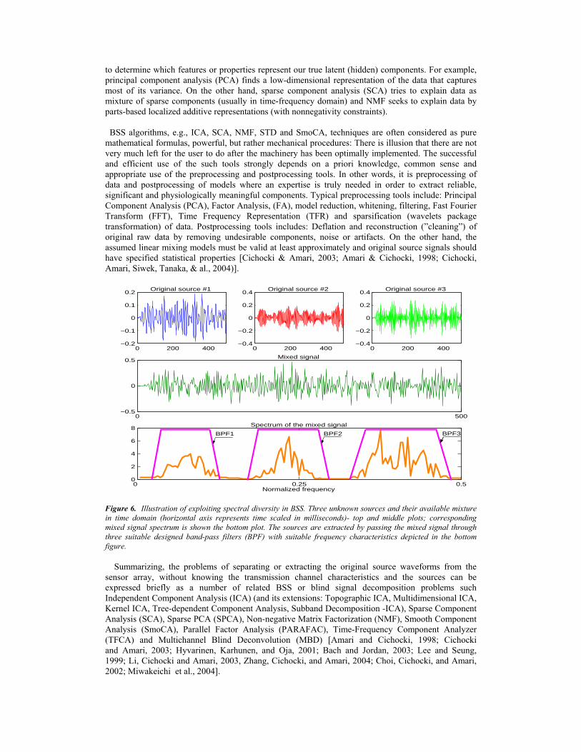
Although many different source separation and multichannel signal decomposition algorithms are available, their principles are generally speaking based on various criteria (See Table 2) and diversities of signals, typically, time, frequency, (spectral or “time coherence”) and/or time-frequency diversities, or more generally, joint space-time-frequency (STF) diversity (see Figs. 6, 7 and 13). For example time frequency diversity leads to concept of Time-Frequency Component Analyzer (TFCA) [Belouchrani & Amin, 1996, Cichocki and Amari, 2003]. TFCA decomposes the signal into specific components in the time-frequency domain and computes the time frequency representations (TFRs) of the individual components. Usually components are interpreted here as localized, sparse and structured signals in the time-frequency plain (spectrogram). In other words, in TFCA components are estimated by analyzing the time-frequency distribution of the observed signals. TFCA provides an elegant and promising solution to suppression of some artifacts and interference via masking and/or filtering of undesired - components. Moreover, estimated components S or Y represent usually unknown source signals with specific statistical properties or temporal structures. The matrices (see Eq. (1)) have usually clear statistical properties and meanings. For example, the rows of the matrix S that represent estimated sources or components should be as sparse as possible for sparse component analysis (SCA) or statistically mutually independent as possible for independent component analysis (ICA). Often it is required that the estimated components are piecewise smooth for smooth component analysis (SmoCA) or take only nonnegative values for nonnegative matrix factorization (NMF) or values with specific constraints [Lee and Seung, 1999; Cichocki and Georgiev, 2003]. More sophisticated or advanced approaches use combinations or integration of various criteria such as independence, sparsity, smoothness, decorrelation and principles based on second order statistics, nonstationarity, higher order statistics, nongaussianity etc. in order to separate or extract sources with various statistical properties and to reduce the influence of noise and undesirable interference. The all above mentioned BSS methods belongs to a wide class of unsupervised learning algorithms. Unsupervised learning techniques try to discover a structure underlying a data set, extraction of meaningful features and finding useful representations of the given data [Li, Cichocki and Amari, 2002, 2003]. Since data can be always interpreted in many different ways, some knowledge is needed

to determine which features or properties represent our true latent (hidden) components. For example, principal component analysis (PCA) finds a low-dimensional representation of the data that captures most of its variance. On the other hand, sparse component analysis (SCA) tries to explain data as mixture of sparse components (usually in time-frequency domain) and NMF seeks to explain data by parts-based localized additive representations (with nonnegativity constraints). BSS algorithms, e.g., ICA, SCA, NMF, STD and SmoCA, techniques are often considered as pure mathematical formulas, powerful, but rather mechanical procedures: There is illusion that there are not very much left for the user to do after the machinery has been optimally implemented. The successful and efficient use of the such tools strongly depends on a priori knowledge, common sense and appropriate use of the preprocessing and postprocessing tools. In other words, it is preprocessing of data and postprocessing of models where an expertise is truly needed in order to extract reliable, significant and physiologically meaningful components. Typical preprocessing tools include: Principal Component Analysis (PCA), Factor Analysis, (FA), model reduction, whitening, filtering, Fast Fourier Transform (FFT), Time Frequency Representation (TFR) and sparsification (wavelets package transformation) of data. Postprocessing tools includes: Deflation and reconstruction (”cleaning”) of original raw data by removing undesirable components, noise or artifacts. On the other hand, the assumed linear mixing models must be valid at least approximately and original source signals should have specified statistical properties [Cichocki & Amari, 2003; Amari & Cichocki, 1998; Cichocki, Amari, Siwek, Tanaka, & al., 2004)].

0 0.25 0.50

2

4

6

8Spectrum of the mixed signal

Normalized frequency

0 200 400−0.2

−0.1

0

0.1

0.2Original source #1

0 200 400−0.4

−0.2

0

0.2

0.4Original source #2

0 200 400−0.4

−0.2

0

0.2

0.4Original source #3

0 500−0.5

0

0.5Mixed signal

BPF3 BPF2 BPF1

Figure 6. Illustration of exploiting spectral diversity in BSS. Three unknown sources and their available mixture in time domain (horizontal axis represents time scaled in milliseconds)- top and middle plots; corresponding mixed signal spectrum is shown the bottom plot. The sources are extracted by passing the mixed signal through three suitable designed band-pass filters (BPF) with suitable frequency characteristics depicted in the bottom figure. Summarizing, the problems of separating or extracting the original source waveforms from the sensor array, without knowing the transmission channel characteristics and the sources can be expressed briefly as a number of related BSS or blind signal decomposition problems such Independent Component Analysis (ICA) (and its extensions: Topographic ICA, Multidimensional ICA, Kernel ICA, Tree-dependent Component Analysis, Subband Decomposition -ICA), Sparse Component Analysis (SCA), Sparse PCA (SPCA), Non-negative Matrix Factorization (NMF), Smooth Component Analysis (SmoCA), Parallel Factor Analysis (PARAFAC), Time-Frequency Component Analyzer (TFCA) and Multichannel Blind Deconvolution (MBD) [Amari and Cichocki, 1998; Cichocki and Amari, 2003; Hyvarinen, Karhunen, and Oja, 2001; Bach and Jordan, 2003; Lee and Seung, 1999; Li, Cichocki and Amari, 2003, Zhang, Cichocki, and Amari, 2004; Choi, Cichocki, and Amari, 2002; Miwakeichi et al., 2004].

(a)

0 75 150 225 300 375 450 525 600−4

−2

0

2

4Mixed signal

0 300 600−1

−0.5

0

0.5

1Original source #3

0 300 600−1

−0.5

0

0.5

1Original source #1

0 300 600−1

−0.5

0

0.5

1Original source #2

(b)

Figure 7. Illustration of a basic principle of the Time-Frequency Component Analyzer (TFCA): Exploiting time-frequency diversity in BSS. (a) Original unknown source signals and available mixed signal (horizontal axis represents time scaled in milliseconds). (b) 3-D Time frequency representation of the mixed signal. Due to non-overlapping time-frequency signatures of the sources by masking and synthesis (inverse transform), we are able to extract the desired sources.

4. Deflation and Filtering of Multidimensional Signals After extracting the independent components or performing blind separation of signals (from the mixture), we can examine the effects of discarding some of components by reconstructing the sensor signals from the remaining components. This procedure is called deflation or reconstruction, and allows us to remove unnecessary (or undesirable) components that are hidden in the mixture (superimposed or overlapped data). In other words, the deflation procedure allows us to extract and remove one or more components (or estimated sources) from the mixture x(k).

The deflation procedure is carried out in two steps.

1. In the first step, the selected algorithm to estimate the demixing (separating or decomposition) matrix W and then performs the decomposition of observations into components by y(k) = W x(k).

2. In the second step, the deflation algorithm eliminates one or more components from the vector y(k) and then performs the back-propagation xr = W+ yr(k), where xr is a vector of reconstructed sensor signals, W+ = Hestim is a generalized pseudo inverse matrix of the estimated demixing matrix W, and yr (k) is the vector obtained from the vector y(k) after removal of all the undesirable components (i.e., by replacing them with zeros). In the special case, when the number of sources is equal to the number of sensors and the number of outputs, we can use the standard inverse matrix W-1 instead of the pseudo-inverse W+.

In batch format, the reconstruction procedure can be written as

Xr = W+ Yr (8)

where

Xr = [ xr(1), xr(2), ..., xr(N) ] - reconstructed sensor signals,

Yr = [ yr(1), yr(2), ..., yr(N) ] - reduced (selected or filtered) independent components.

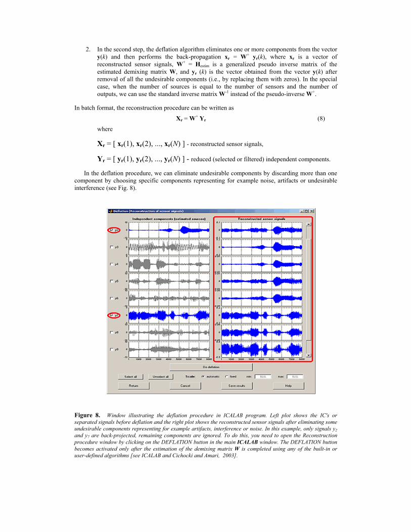
In the deflation procedure, we can eliminate undesirable components by discarding more than one component by choosing specific components representing for example noise, artifacts or undesirable interference (see Fig. 8).

Figure 8. Window illustrating the deflation procedure in ICALAB program. Left plot shows the IC's or separated signals before deflation and the right plot shows the reconstructed sensor signals after eliminating some undesirable components representing for example artifacts, interference or noise. In this example, only signals y2 and y7 are back-projected, remaining components are ignored. To do this, you need to open the Reconstruction procedure window by clicking on the DEFLATION button in the main ICALAB window. The DEFLATION button becomes activated only after the estimation of the demixing matrix W is completed using any of the built-in or user-defined algorithms [see ICALAB and Cichocki and Amari, 2003].

(a)

1x

Wny ��

mxmx

2x

1y

2y 2x

1x

�W

SensorSignals

DemixingSystem

BSS/ICA

InverseSystem

ReconstructedSensorsSignals

ExpertDecision

�

Hardswitches

0 or 1

(b)

(c)

1x

Wny ��

mxmx

2x

1y

2y 2x

1x1y

2y

ny

�W

SensorSignals

DemixingSystem

BSS/ICA

OptionalNonlinearAdaptive

Filters

InverseSystem

ReconstructedSensorsSignals

NAF

NAF

NAF

DecisionBlocks

�

On-lineswitching

0 or 1

1~y

2~y

ny~

W�� �

�W

SensorSignals

ICADemixing

System

Soft SwitchesAdaptive Nonlinearities

InverseSystem

ReconstructedSensorsSignals

SoftDecision

B

-B-B

B

-B

B

Typical Adaptive Nonlinearities

�

x1 y1

x2 y2

xm yn

y1~

y2~

yn~

mx

2x

1x

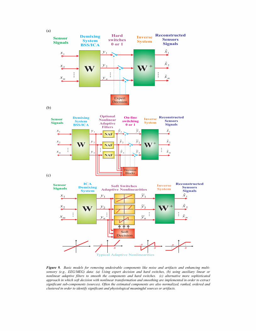
Figure 9. Basic models for removing undesirable components like noise and artifacts and enhancing multi-sensory (e.g., EEG/MEG) data: (a) Using expert decision and hard switches, (b) using auxiliary linear or nonlinear adaptive filters to smooth the components and hard switches. (c) alternative more sophisticated approach in which soft decision with nonlinear transformation and smoothing are implemented in order to extract significant sub-components (sources). Often the estimated components are also normalized, ranked, ordered and clustered in order to identify significant and physiological meaningful sources or artifacts.

The deflation (reconstruction) procedure is illustrated in Fig. 8 for ICALAB package [Cichocki et al 2002]. In this figure, almost all (from 10) components yi are reset to zero except the components y2 and y7 that are projected back to sensor levels (as xr(k) = pinv(W) yr (k) = W+yr(k), where W+ (10x10) means pseudo-inverse of demixing matrix W and yr(k) = [ 0, y2(k), 0, 0, 0, 0, y7(k), 0, 0, 0 ]T). The results are shown on right-side plot in Fig. 8. In many cases the estimated components must be at first filtered or smoothed in order to identify all significant components.

In addition to the denoising and artifacts removal, BSS techniques can be used to decompose EEG/MEG data into individual components, each representing a physiologically distinct process or brain source. The main idea here is to apply localization and imaging methods to each of these components in turn. The decomposition is usually based on the underlying assumption of sparsity and/or statistical independence between the activation of different cell assemblies involved. Alternative criteria for the decomposition are spatio-temporal decorrelation, temporal predictability or smoothness of components. The BSS or more general BSP approaches are promising methods for the blind extraction of useful signals from the EEG/MEG data. The EEG/MEG data can be first decomposed into useful signal and noise subspaces using standard techniques PCA, SPCA or Factor Analysis (FA) and standard filtering. Next, we apply BSS algorithms to decompose the observed signals (signal subspace) into specific components. The BSS approaches enable us to project each component (localized “brain source”) onto an activation map at the skull level. For each activation map, we can apply an EEG/MEG source localization procedure, looking only for a single dipole (or brain source) per map. By localizing multiple sources independently, we can dramatically reduce the computational complexity and increase the likelihood of efficiently converging to the correct and reliable solution.

One of the biggest strength of BSS approach is that it offers a variety of powerful and efficient algorithms that are able to estimate various kinds of sources (sparse, independent, spatio-temporally decorrelated, smooth etc.). Some of the algorithms, e.g., AMUSE or TICA [Cichocki & Amari, 2003; Cruces & Cichocki, 2003; Choi, Cichocki, & Amari, 1998a], are able to automatically rank and order the component according to their complexity or sparseness measures. Some algorithms are very robust in respect to noise (e.g., SOBI or SONS) [Choi et al., 2002, 2002; Choi, Cichocki, & Amari, 1998b]. In some cases, it is recommended to use algorithms in cascade (multiple) or parallel mode in order to extract components with various features and statistical properties [Hyvarinen, Karhunen and Oja, 2001, Cichocki and Amari, 2003].

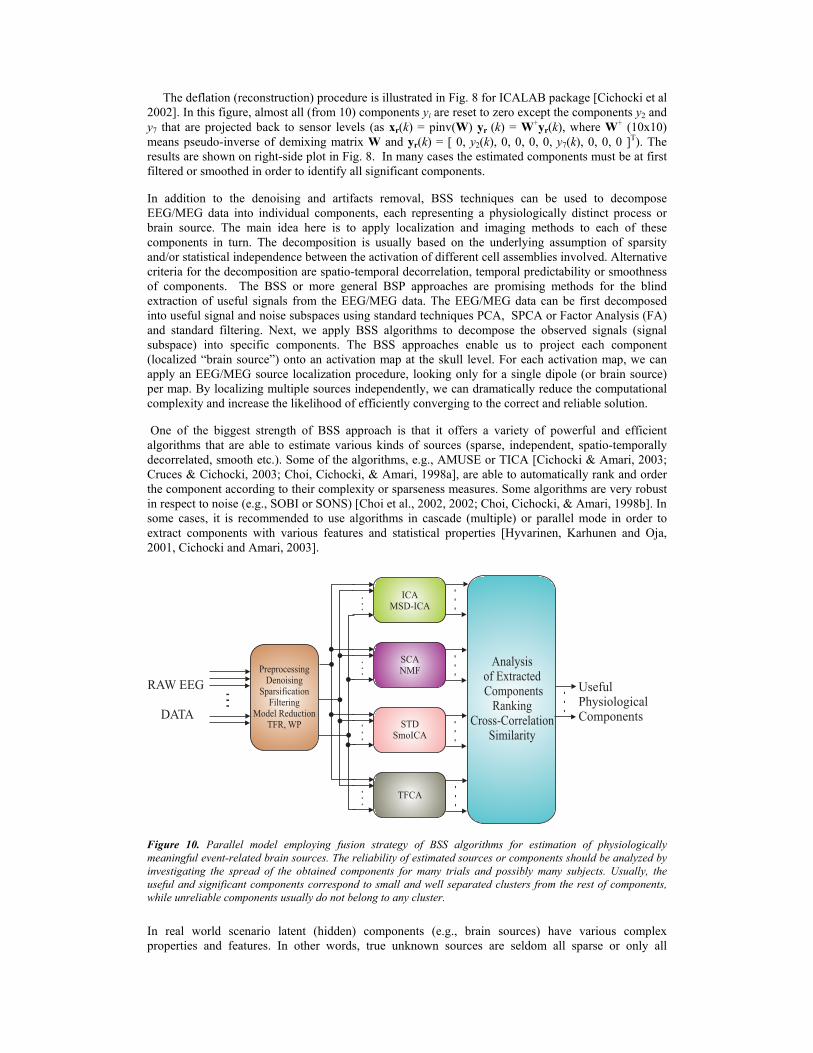
Figure 10. Parallel model employing fusion strategy of BSS algorithms for estimation of physiologically meaningful event-related brain sources. The reliability of estimated sources or components should be analyzed by investigating the spread of the obtained components for many trials and possibly many subjects. Usually, the useful and significant components correspond to small and well separated clusters from the rest of components, while unreliable components usually do not belong to any cluster.

In real world scenario latent (hidden) components (e.g., brain sources) have various complex properties and features. In other words, true unknown sources are seldom all sparse or only all

statistically independent, or all spatio-temporally decorrelated. Thus, if we apply only one single technique like ICA or SCA or STD we usually fail to extract all hidden components. We need rather to apply fusion strategy or combination of several criteria and associated algorithms to extract all desired sources. We may apply here two possible approaches. The most promising approach is a sequential blind extraction in which we extract components one by one in each stage applying different criterion. (e.g., statistical independence, sparseness. smoothness etc). In this way, we can extract sequentially different components with various properties. In alternative approach, after suitable preprocessing, we perform simultaneously (in parallel way) several BSS methods (ICA, SCA, STD, TFCA). Next the estimated components are normalized, ranked, clustered and compared to each other using some similarity measures (see Fig. 10). Furthermore, the components are back projected to scalp level and brain sources are localized on basis of clusters of subcomponents. In this way, on basis of a priori knowledge (e.g., information about external stimuli for event related brain sources), we can identify components with some electrophysiological meaning and specific localizations.

In summary, blind source separation and generalized component analysis (BSS/GCA) algorithms allows:

1. Extract and remove artifacts and noise from raw EEG/MEG data. 2. Recover neuronal brain sources activated in cortex (especially, in auditory, visual, somato-

sensory, motoric and olfactory cortex). 3. Improve the signal-to-noise ratio (SNR) of evoked potentials (EP’s), especially AEP, VEP

and SEP. 4. Improve spatial resolution of EEG and reduce level of subjectivity involved in the brain

source localization. 5. Extract features and hidden brain patterns and classify them.

Applications of BSS show special promise in the areas of non-invasive human brain imaging techniques to delineate the neural processes that underlie human cognition and sensoro-motor functions. These approaches lead to interesting and exciting new ways of investigating and analyzing brain data and develop new hypotheses how the neural assemblies communicate and process information. This is actually an extensive and potentially promising research area. However, these techniques and methods still remain to be validated at least experimentally to obtain full gain of the presented approach. The fundamental problems here are: What are the system’s real properties and how can we get information about them? What is valuable information in the observed data and what is only noise or interference? How can the observed (sensor) data be transformed into features characterizing the brain sources in a reasonable way? 5. Early Detection of Alzheimer Disease using Blind Signal Decomposition Finding electro-physiological signal or neuroimaging markers of different diseases and psychiatric disorders is generating increasing interest [Jeong, 2004; Petersen et al., 2001, Babiloni et al..Aug. 2004]. The prevalence of dementia, a clinical disorder associated with Alzheimer’s disease (AD) and other kind of dementia such vascular dementia, is steadily increasing. Recent advances in drug treatment for dementia, particularly the acetylcholinesterase inhibitors for Alzheimer’s disease (AD), are most effective in early stages which are difficult to accurately diagnosis. Therefore, accurate early diagnosis is needed to ensure effective pharmacological interventions in dementia cases [Musha et al., 2002; Petersen, 2003]. Alzheimer disease (AD) is one of the most frequent dementia among the elderly population [Petersen, 2003; Jeong, 2004; DeKosky & Marek, 2003]. Recent studies have demonstrated that AD has a presymptomatic phase, likely lasting years, during which neuronal degeneration is occurring but clinical symptoms are not clearly observable. This makes preclinical discrimination between people who will and will not ultimately develop AD very important and critical for early treatment of the disease which could prevent or at least slow down the onset of clinical manifestations of disease. A diagnostic method should be inexpensive to make possible screening of many individuals who are at risk of developing this dangerous disease. The electroencephalogram (EEG) is one of the most promising candidates to become such a method since it is cheap, portable and noninvasive recording of EEG data is relatively simple. However, while quite many signal processing techniques have been already applied for revealing pathological changes in EEG associated with AD (see [Jeong, 2004; Petersen, 2003; Cichocki et al., 2004], for review), the EEG-based detection of AD

at its most early stages is still not sufficiently reliable and further improvements are necessary. Moreover, the efficiency of early detection of AD is lower for standard EEG comparing to modern neuroimaging techniques (fMRI, PET, SPECT) and it is considered only as an additional diagnostic tool [Wagner, 2000; DeKosky & Marek, 2003]. This is why a number of more sophisticated or more advanced multistage data analysis approaches with optimization should be applied for this problem. There is still some variety of unexplored and more advanced blind signal and image processing methods to find more data oriented and, thus, better discriminating approaches and to our best knowledge, no study till now investigated the application of BSS and ICA methods as preprocessing tools in AD diagnosis [Cichocki et al, 2005]. Generally speaking, in our novel approach, we first decompose EEG data into suitable components (e.g., independent, sparse, smooth and/or spatio-temporal decorrelated), next we rank them according to some measures (such as linear predictability/increasing complexity or sparseness) and then we project to the scalp level only some significant very specific ranked components, possibly of physiological origin that could be apparently the brain signal markers for dementia, and more specifically, for Alzheimer disease. We believe that BSS/ICA are promising methods for discrimination dementia due the following reasons (see Fig. 11):

1) First of all, ICA and BSS algorithms allow us to extract and eliminate various artifacts and high frequency noise and interference.

2) Second, novel BSS algorithms, especially these with equivariant and nonholonomic properties

allow us to extract extremely weak brain sources [Cichocki et al., 1994; Cichocki & Amari, 2003], probably corresponding to the brain sources located deep in the brain like, e.g., in the hippocampus.

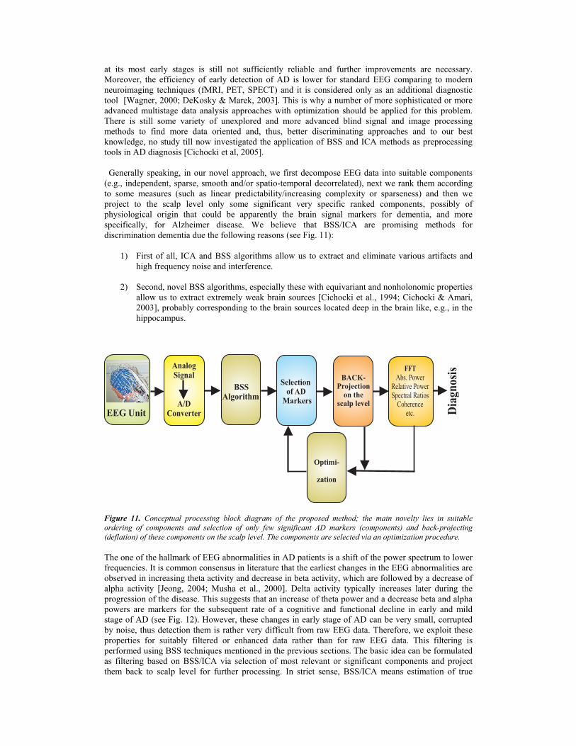
Figure 11. Conceptual processing block diagram of the proposed method; the main novelty lies in suitable ordering of components and selection of only few significant AD markers (components) and back-projecting (deflation) of these components on the scalp level. The components are selected via an optimization procedure. The one of the hallmark of EEG abnormalities in AD patients is a shift of the power spectrum to lower frequencies. It is common consensus in literature that the earliest changes in the EEG abnormalities are observed in increasing theta activity and decrease in beta activity, which are followed by a decrease of alpha activity [Jeong, 2004; Musha et al., 2000]. Delta activity typically increases later during the progression of the disease. This suggests that an increase of theta power and a decrease beta and alpha powers are markers for the subsequent rate of a cognitive and functional decline in early and mild stage of AD (see Fig. 12). However, these changes in early stage of AD can be very small, corrupted by noise, thus detection them is rather very difficult from raw EEG data. Therefore, we exploit these properties for suitably filtered or enhanced data rather than for raw EEG data. This filtering is performed using BSS techniques mentioned in the previous sections. The basic idea can be formulated as filtering based on BSS/ICA via selection of most relevant or significant components and project them back to scalp level for further processing. In strict sense, BSS/ICA means estimation of true

(original) neuronal brain sources, though exactly the same procedure can be used for separation of two or more subspaces of the signal without estimation of true sources. One procedure currently becoming popular in EEG analysis is removing artifact-related BSS components and back projection of components originating from brain [Jung et al., 2000; Vorobyov & Cichocki, 2002]. In this procedure, components of brain origin are not required to be separated from each other exactly, because they are mixed again by back projection after removing artifact-related components. But by the similar procedure, we can filter the on going ”brain noise” also in wider sense, improving the signal to noise ratio (SNR). In one of our simplest developed procedure, we do not attempt to identify individual brain sources or physiologically meaningful components but rather identify the whole group or cluster of significant for AD components. In other words, we divide the available EEG data into two subspaces: brain signal subspace and “brain noise” subspace. Finding fundamental mechanism or principle for identification of significant and not significant components is critical in our approach and, in general, may require extensive studies. We attempt to differentiate clusters or subspaces of components with similar properties or features. In this simple approach the estimation of all individual components corresponding to separate and meaningful brain sources is not required, unlike in other applications of BSS to EEG processing (including its most popular variant, employing standard ICA)). The use of clusters of components could be especially beneficial when the data from different subjects are compared: similarities among individual components in different subjects are usually low, while subspaces formed by similar components are more likely to be sufficiently consistent. Differentiation of subspaces with high and low amount of diagnostically useful information can be made easier if components are separated and sorted according to some criteria which, at least to some extent, correlate with the diagnostic value of components. For this reason we have applied AMUSE BSS algorithm which provides automatic ordering of components according to decreasing variance and decreasing their linear predictability.

AMUSE [Tong et al., 1991, 1993; Szupiluk and Cichocki, 2001; Cichocki and Amari, 2003] is a BSS algorithm which arranges components not only in the order of decreasing variance (that is typical for the use of singular value decomposition (SVD) which is implemented within the algorithm), but also in the order of their decreased linear predictability. Low values for both characteristics can be specific for many of EEG components related to high frequency artifacts, especially electromyographic signal (which cannot be sufficiently removed by usual filtering in frequency domain. Thus, a first attempt of selection of diagnostically important components can be made by removing a range of components separated with AMUSE (below referred to as "AMUSE components") with the lowest linear predictability. Automatic sorting of components by this algorithm makes it possible to do this simply by removing components with indices higher than some chosen value.

5.1 AMUSE Algorithm and its Properties AMUSE algorithm belongs to the group of second-order-statistics spatio-temporal decorrelation (SOS-STD) BSS algorithms. It provides similar decomposition as the well known and popular SOBI algorithms [Belouchrani et al., 1997; Tang et al. 2002]. AMUSE algorithm uses simple principles that the estimated components should be spatio-temporally decorrelated and be less complex (i.e., have better linear predictability) than any mixture of those sources. The components are ordered according to decreasing values of singular values of a time-delayed covariance matrix. As in PCA (Principal Component Analysis) and unlike in many ICA algorithms, all components estimated by AMUSE are uniquely defined (i.e., any run of algorithms on the same data will always produce the same components) and consistently ranked.

AMUSE algorithm can be considered as two consecutive PCAs: First, PCA is applied to input data; secondly, PCA (SVD) is applied to the time-delayed covariance matrix of the output of previous stage. In the first step standard or robust prewhitening (sphering) is applied as a linear transformation

z(t) = Qx(t), where 12

x−=Q R of the standard covariance matrix ( ) ( ){ }T

x t t=R x xE and x(t) is a

vector of observed data for time instant t. Next, SVD is applied to a time-delayed covariance matrix of pre-whitened data: ( ) ( ){ }1T T

z t t= − = ΣR z z U VE , where Σ is a diagonal matrix with

decreasing singular values and U, V are matrices of eigenvectors. Then, an demixing (separating) matrix is estimated as 1ˆ T−= =W H U Q or ˆ T=H Q U .

AMUSE algorithm is much faster than the vast majority of BSS algorithms (its processing speed is mainly defined by the PCA processing within it) and is very easy to use, because no parameters are required. It is implemented as a part of package "ICALAB for signal processing" [Cichocki et al.,

online] freely available online and can be called also from current version of EEGLAB toolbox [Delorme and Makeig, 2004) (which is freely available online at http://www.sccn.ucsd.edu/eeglab/) if both toolboxes are installed.

5.2. Preliminary Results

The main advantage of AMUSE over other BSS algorithms was highly reproducible components in respect to their ranking or ordering and also across subjects belonging to the same of group of patients. This allows us to identify significant components and optimize their number. (a) (b)

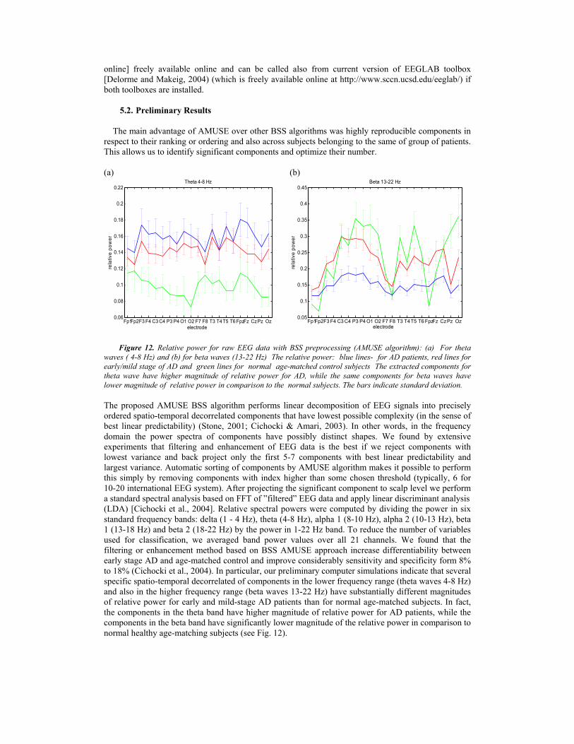
Figure 12. Relative power for raw EEG data with BSS preprocessing (AMUSE algorithm): (a) For theta waves ( 4-8 Hz) and (b) for beta waves (13-22 Hz) The relative power: blue lines- for AD patients, red lines for early/mild stage of AD and green lines for normal age-matched control subjects The extracted components for theta wave have higher magnitude of relative power for AD, while the same components for beta waves have lower magnitude of relative power in comparison to the normal subjects. The bars indicate standard deviation. The proposed AMUSE BSS algorithm performs linear decomposition of EEG signals into precisely ordered spatio-temporal decorrelated components that have lowest possible complexity (in the sense of best linear predictability) (Stone, 2001; Cichocki & Amari, 2003). In other words, in the frequency domain the power spectra of components have possibly distinct shapes. We found by extensive experiments that filtering and enhancement of EEG data is the best if we reject components with lowest variance and back project only the first 5-7 components with best linear predictability and largest variance. Automatic sorting of components by AMUSE algorithm makes it possible to perform this simply by removing components with index higher than some chosen threshold (typically, 6 for 10-20 international EEG system). After projecting the significant component to scalp level we perform a standard spectral analysis based on FFT of ”filtered” EEG data and apply linear discriminant analysis (LDA) [Cichocki et al., 2004]. Relative spectral powers were computed by dividing the power in six standard frequency bands: delta (1 - 4 Hz), theta (4-8 Hz), alpha 1 (8-10 Hz), alpha 2 (10-13 Hz), beta 1 (13-18 Hz) and beta 2 (18-22 Hz) by the power in 1-22 Hz band. To reduce the number of variables used for classification, we averaged band power values over all 21 channels. We found that the filtering or enhancement method based on BSS AMUSE approach increase differentiability between early stage AD and age-matched control and improve considerably sensitivity and specificity form 8% to 18% (Cichocki et al., 2004). In particular, our preliminary computer simulations indicate that several specific spatio-temporal decorrelated of components in the lower frequency range (theta waves 4-8 Hz) and also in the higher frequency range (beta waves 13-22 Hz) have substantially different magnitudes of relative power for early and mild-stage AD patients than for normal age-matched subjects. In fact, the components in the theta band have higher magnitude of relative power for AD patients, while the components in the beta band have significantly lower magnitude of the relative power in comparison to normal healthy age-matching subjects (see Fig. 12).

Fp1Fp2F3 F4 C3 C4 P3 P4 O1 O2 F7 F8 T3 T4T5 T6 FpzFz Cz Pz Oz0.06

0.08

0.1

0.12

0.14

0.16

0.18

0.2

0.22Theta 4-8 Hz

electrode

rela

tive

pow

er

Fp1Fp2F3 F4 C3 C4 P3 P4 O1 O2 F7 F8 T3 T4T5 T6 FpzFz Cz Pz Oz0.05

0.1

0.15

0.2

0.25

0.3

0.35

0.4

0.45Beta 13-22 Hz

electrode

rela

tive

pow

er

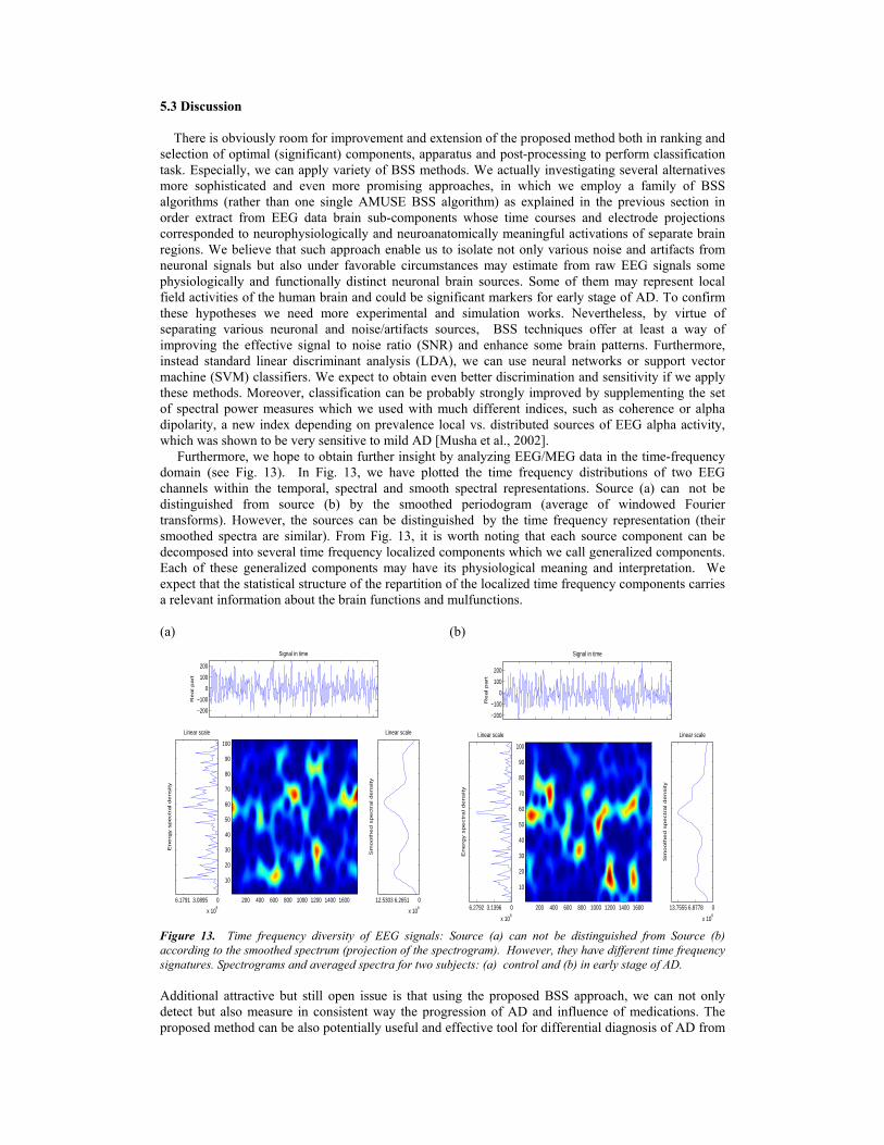
5.3 Discussion There is obviously room for improvement and extension of the proposed method both in ranking and selection of optimal (significant) components, apparatus and post-processing to perform classification task. Especially, we can apply variety of BSS methods. We actually investigating several alternatives more sophisticated and even more promising approaches, in which we employ a family of BSS algorithms (rather than one single AMUSE BSS algorithm) as explained in the previous section in order extract from EEG data brain sub-components whose time courses and electrode projections corresponded to neurophysiologically and neuroanatomically meaningful activations of separate brain regions. We believe that such approach enable us to isolate not only various noise and artifacts from neuronal signals but also under favorable circumstances may estimate from raw EEG signals some physiologically and functionally distinct neuronal brain sources. Some of them may represent local field activities of the human brain and could be significant markers for early stage of AD. To confirm these hypotheses we need more experimental and simulation works. Nevertheless, by virtue of separating various neuronal and noise/artifacts sources, BSS techniques offer at least a way of improving the effective signal to noise ratio (SNR) and enhance some brain patterns. Furthermore, instead standard linear discriminant analysis (LDA), we can use neural networks or support vector machine (SVM) classifiers. We expect to obtain even better discrimination and sensitivity if we apply these methods. Moreover, classification can be probably strongly improved by supplementing the set of spectral power measures which we used with much different indices, such as coherence or alpha dipolarity, a new index depending on prevalence local vs. distributed sources of EEG alpha activity, which was shown to be very sensitive to mild AD [Musha et al., 2002]. Furthermore, we hope to obtain further insight by analyzing EEG/MEG data in the time-frequency domain (see Fig. 13). In Fig. 13, we have plotted the time frequency distributions of two EEG channels within the temporal, spectral and smooth spectral representations. Source (a) can not be distinguished from source (b) by the smoothed periodogram (average of windowed Fourier transforms). However, the sources can be distinguished by the time frequency representation (their smoothed spectra are similar). From Fig. 13, it is worth noting that each source component can be decomposed into several time frequency localized components which we call generalized components. Each of these generalized components may have its physiological meaning and interpretation. We expect that the statistical structure of the repartition of the localized time frequency components carries a relevant information about the brain functions and mulfunctions. (a) (b)

Figure 13. Time frequency diversity of EEG signals: Source (a) can not be distinguished from Source (b) according to the smoothed spectrum (projection of the spectrogram). However, they have different time frequency signatures. Spectrograms and averaged spectra for two subjects: (a) control and (b) in early stage of AD. Additional attractive but still open issue is that using the proposed BSS approach, we can not only detect but also measure in consistent way the progression of AD and influence of medications. The proposed method can be also potentially useful and effective tool for differential diagnosis of AD from

−200

−100

0

100

200

Re

al p

art

Signal in time

03.08956.1791

x 108

Linear scale

En

erg

y s

pe

ctr

al d

en

sity

200 400 600 800 1000 1200 1400 1600

10

20

30

40

50

60

70

80

90

100

06.265112.5303

x 106

Linear scale

Sm

oo

the

d s

pe

ctr

al d

en

sity

−200

−100

0

100

200

Real part

Signal in time

03.13966.2792

x 108

Linear scale

Energ

y s

pectr

al density

200 400 600 800 1000 1200 1400 1600

10

20

30

40

50

60

70

80

90

100

06.877813.7555

x 106

Linear scale

Sm

ooth

ed s

pectr

al density

other types of dementia, and possibly for diagnosis of other diseases. Particularly, the possibility of differential diagnosis of AD from vascular dementia (VaD) will be very important. Other areas of EEG analysis can be also possible field for the application of our preprocessing technique. For these purposes, more studies would be needed to asses the impact of the available and future blind source separation methods for enhancement/filtering and extraction of the EEG/MEG, fMRI signals of interest.

6. Conclusion In this paper we have discussed briefly several linear models for blind source separation and emerging signal decomposition approaches in application to analysis and preprocessing of EEG and MEG data. These techniques are potentially useful not only for noise reduction and artifacts removal, but also in source localization and improving spatial resolution of EEG. Furthermore, we have discussed the BSS approach for blind extraction from raw EEG data specific components in order to improve sensitivity and specificity of early detection of Alzheimer’s disease. The basic principle is to order and cluster automatically of the estimated components and next project back to the scalp level only the suitable group of components which are significant electrophysiological markers of Alzheimer disease. The suboptimal selection of indexes and the number of ordered components has been performed by extensive computer simulation and optimization procedure. References Amari, S., & Cichocki, A. (1998). Adaptive blind signal processing - neural network approaches. Proceedings IEEE, 86, 1186–1187.

Amari, S., Hyvarinem, A., Lee, S., Lee, T., & Sanchez, V. (2002). Blind signal separation and independent component analysis. Neurocomputing, 49 (12), 1-5.

Babiloni C., Miniussi C. , Moretti D., Vecchio F., Salinari S. , Frisoni G. and Rossini P.M., Cortical Networks Generating Movement-Related EEG Rhythms in Alzheimer's Disease: An EEG Coherence Study, Behavioral Neuroscience, Volume 118, Issue 4, Aug. 2004, 698-706. Babiloni, F., Babiloni, C., Carducci, F., Romani, G.L., Rossini, P.M., Angelone, L.M., and Cincotti, F. (2004). Multimodal Integration of EEG and MEG data: A Simulation Study with Variable Signal to Noise Ratio and Number of Sensors. Human Brain Mapping 22: 52-64.

Bach, F., & Jordan, M. (2003). Beyond independent components: trees and clusters. Journal of Machine Learning Research, 4, 1205-1233.

Barros, A. K., & Cichocki, A. (2001). Extraction of specific signals with temporal structure. Neural Computation, 13 (9), 1995-2000.

Bell, A., & Sejnowski, T. (1995). An information maximization approach to blind separation and blind deconvolution. Neural Computation, 7, no. 6, 1129-1159.

Belouchrani, A., Abed-Meraim, K., Cardoso, J.-F., & Moulines, ´E. (1997). A blind source separation technique using second-order statistics. IEEE Trans. Signal Processing, 45 (2), 434-444.

Belouchrani, A., & Amin, M. (1996). A new approach for blind source separation using timefrequency distributions. Proc. SPIE, 2846, 193-203.

Belouchrani, A., & Cichocki, A. (2000). Robust whitening procedure in blind source separation context. Electronics Letters, 36 (24), 2050-2053.

Choi, S., Cichocki, A., & Amari, S. (2002). Equivariant nonstationary source separation. Neural Networks, 15, 121–130.

Choi, S., Cichocki, A., & Belouchrani, A. (2002). Second order nonstationary source separation. Journal of VLSI Signal Processing, 32 (1–2), 93–104.

Cichocki, A., & Amari, S. (2003). Adaptive Blind Signal and Image Processing (new revised and improved edition). New York: John Wiley.

Cichocki, A., Amari, S. M., Siwek, K., Tanaka, T., & al. et. (2004). ICALAB toolboxes for signal and image processing available on lline www.bsp.brain.riken.go.jp. JAPAN.

Cichocki, A., & Belouchrani, A. (2001). Sources separation of temporally correlated sources from noisy data using bank of band-pass filters. In Third International Conference on Independent Component Analysis and Signal Separation (ICA-2001) (pp. 173–178). San Diego, USA.

Cichocki, A., Bogner, R., Moszczynski, L., & Pope, K. (1997). Modified H´erault-Jutten algorithms for blind separation of sources. Digital Signal Processing, 7 (2), 80 - 93.

Cichocki, A., & Georgiev, P. (2003). Blind source separation algorithms with matrix constraints. IEICE Transactions on Fundamentals of Electronics, Communications and Computer Sciences, E86-A(1), 522–531.

Cichocki, A., Kasprzak, W., & Skarbek, W. (1996). Adaptive learning algorithm for principal component analysis with partial data. In R. Trappl (Ed.), Cybernetics and systems ’96. thirteenth european meeting on cybernetics and systems research (Vol. 2, pp. 1014–1019). Austrian Society for Cybernetic Studies, Vienna.

Cichocki, A., Li, Y., Georgiev, P. G., & Amari, S. (2004). Beyond ICA: Robust sparse signal representations. In Proceedings of 2004 IEEE International Symposium on Circuits and Systems (ISCAS2004) (Vol. V, pp. 684–687). Vancouver, Canada.

Cichocki, A., Rutkowski, T. M., & Siwek, K. (2002). Blind signal extraction of signals with specified frequency band. In Neural Networks for Signal Processing XII: Proceedings of the 2002 IEEESignal Processing Society Workshop (pp. 515–524). Martigny, Switzerland: IEEE.

Cichocki, A., Shishkin, S., Musha, T., Leonowicz, Z., Asada, T., & Kurachi, T. (2005). EEG filtering based on blind source separation (BSS) for early detection of Alzheimer disease. In Clinical Neurophysiology (p. (in press)).

Cichocki, A., & Thawonmas, R. (2000). On-line algorithm for blind signal extraction of arbitrarily distributed, but temporally correlated sources using second order statistics. Neural Processing Letters, 12 (1), 91-98.

Cichocki, A., Thawonmas, R., & Amari, S. (1997). Sequential blind signal extraction in order specified by stochastic properties. Electronics Letters, 33 (1), 64-65.

Cichocki, A., & Unbehauen, R. (1993). Robust estimation of principal components in real time.Electronics Letters, 29 (21), 1869–1870.

Cichocki, A., & Unbehauen, R. (1994). Neural Networks for Optimization and Signal Processing (new revised and improved edition). New York: John Wiley & Sons.

Cichocki, A., & Unbehauen, R. (1996). Robust neural networks with on-line learning for blind identification and blind separation of sources. IEEE Trans. Circuits and Systems I : Fundamentals Theory and Applications, 43 (11), 894-906.

Cichocki, A., Unbehauen, R., & Rummert, E. (1994). Robust learning algorithm for blind separation of signals. Electronics Letters, 30 (17), 1386-1387.

Cruces, S., Cichocki, A., & Castedo, L. (2000). An iterative inversion approach to blind source separation. IEEE Trans. on Neural Networks, 11 (6), 1423-1437.

Cruces, S. A., Castedo, L., & Cichocki, A. (2002). Robust blind source separation algorithms using cumulants. Neurocomputing, 49, 87–118.

Cruces, S. A., & Cichocki, A. (2003). Combining blind source extraction with joint approximate diagonalization: Thin algorithms for ICA. In Proceedings of 4th International Symposium on Independent Component Analysis and Blind Signal Separation (ICA2003) (pp. 463–468). Kyoto, Japan: ICA.

DeKosky, S., & Marek, K. (2003). Looking backward to move forward: Early detection of neurodegenerative disorders. Science, 302 (5646), 830-834.

Delorme, A., & Makeig, S. (2004). EEGLAB: an open source toolbox for analysis of single-trial EEG dynamics. J. Neuroscience Methods, 134:9-21, 2004, 134, 9-21.

Donoho, D. L., & Elad, M. (2004). Representation via l1 minimization. The Proc. National Academy of Science, 100, 2197-2202.

Fiori, S. (2003). A fully multiplicative orthoghonal-group ICA neural algorithm. Electronics Letters, 39 (24), 1737-1738.

Georgiev, P. G., & Cichocki, A. (2004). Sparse component analysis of overcomplete mixtures by improved basis pursuit method. In Proceedings of 2004 IEEE International Symposium on Circuits and Systems (ISCAS2004) (Vol. V, pp. 37–40). Vancouver, Canada.

Gharieb, R. R., & Cichocki, A. (2003). Second-order statistics based blind source separation using a bank of subband filters. Digital Signal Processing, 13, 252–274.

Himberg, J., Hyvarinen, A., & Esposito, F. (2004). Validating the independent components of neuroimaging time series via clustering and visualization. NeuroImage, 22 (3), 1214-1222.

Hyvarinen, A., Karhunen, J., & Oja, E. (2001). Independent Component Analysis. New York: John Wiley.

Jahn, O., Cichocki, A., Ioannides, A., & Amari, S. (1999). Identification and elimination of artifacts from MEG signals using efficient independent components analysis. In Proc. of th 11th Int. Conference on Biomagentism BIOMAG-98 (p. 224-227). Sendai, Japan.

Jelic, V., Johansson, S., Almkvist, O., Shigeta, M., Julin, P., Nordberg, A., Winblad, B., & Wahlund, L. (2000). Quantitative electroencephalography in mild cognitive impairment: longitudinalchanges and possible prediction of Alzheimer’s disease. Neurobiological Aging, 21 (4), 533-540.

Jeong, J. (2004). EEG dynamics in patients with Alzheimer’s disease. Clinical Neurophysiology,115 (7), 1490-1505.

Jung, H.-Y., & Lee, S.-Y. (2000). On the temporal decorrelation of feature parameters for noiserobustspeech recognition. IEEE Transactions on Speech and Audio Processing, 8 (7), 407-416.

Jung, T., Makeig, S., Humphries, C., Lee, T.-W., McKeown, M., Iragui, V., & Sejnowski, T. (2000). Removing electroencephalographic artifacts by blind source separation. Psychophysiology, 37, 167-178.

Kreutz-Delgado, K., Murray, J. F., Rao, B. D., Engan, K., Lee, T.-W., & Sejnowski, T. J. (2003). Dictionary learning algorithms for sparse representation. Neural Computation, 15 (2), 349-396.

Lee, D. D., & Seung, H. S. (1999). Learning of the parts of objects by non-negative matrix factorization. Nature, 401, 788-791.

Li, Y., Cichocki, A., & Amari, S. (2004). Analysis of sparse representation and blind source separation. Neural Computation, 16 (6), 1193–1204.

Li, Y., Cichocki, A., Amari, S., Shishkin, S., Cao, J., & Gu, F. (2003). Sparse representation and its applications in blind source separation. In Seventeenth Annual Conference on Neural Information Processing Systems (NIPS-2003). Vancouver.

Mainecke, F., Ziehe, A., Kawanabe, M., & M¨uller, K.-R. (2002). A resampling approach to estimate the stability of one dimensional or multidimensional independent components. NeuroImage, 49 (13), 1514-1525.

Makeig, S., Debener, S., Onton, J., & Delorme, A. (2004). Mining event-related brain dynamics. Trends in Cognitive Science, 8, 204-210.

Makeig, S., Delorme, A., M., M. W., Townsend, J., Courchense, E., & Sejnowski, T. (2004). Electroencephalographic brain dynamics following visual targets requiring manual responses. PLOS Biology, (in press).

Malmivuo J, Plonsey R. Bioelectromagnetism: Principles and Application of Bioelectric and Biomagnetic Fields. Oxford University Press, New York, 1995.

Matsuoka, K., Ohya, M., & Kawamoto, M. (1995). A neural net for blind separation of nonstationarysignals. Neural Networks, 8 (3), 411-419.

Miwakeichi, F., Martnez-Montes, E., Valds-Sosa, P. A., Nishiyama, N., Mizuhara, H., & Yamaguchi, Y. (2004). Decomposing EEG data into space-time-frequency components using Parallel Factor Analysis. NeuroImage, 22 (3), 1035-1045.

Molgedey, L., & Schuster, H. (1994). Separation of a mixture of independent signals using time delayed correlations. Physical Review Letters, 72 (23), 3634-3637.

Musha, T., Asada, T., Yamashita, F., T., T. K., Chen, Z., Matsuda, H., Uno, M., & Shankle, W. (2002). A new EEG method for estimating cortical neuronal impairment that is sensitive to early stage Alzheimer’s disease. Clinical Neurophysiology, 113 (7), 1052-1508.

Petersen, R. (2003). Mild Cognitive Impairment: Aging to Alzheimers Disease. New York: Oxford University Press.

Petersen, R., Stevens, J., Ganguli, M., Tangalos, E., Cummings, J., & DeKosky, S. (2001). Practice parameter: Early detection of dementia: Mild cognitive impairment (an evidence-based review). Neurology, 56, 1133-1142.

Rosipal, R., Girolami, M., Trejo, L. J., & Cichocki, A. (2001). Kernel PCA for feature extraction and de-noising in nonlinear regression. Neural Computing & Applications, 10, 231–243.

Sajda, P., Du, S., & Parra, L. (2003). Recovery of constituent spectra using non-negative matrix factorization. In Proceedings of SPIE – volume 5207) (p. 321-331). Wavelets: Applications in Signal and Image Processing.

Stone, J. (2001). Blind source separation using temporal predictability. Neural Computation, 13 (7), 1559-1574. Szupiluk R, Cichocki A. Blind signal separation using second order statistics. Proc. of SPETO 2001, pp. 485-488. Tanaka, T., & Cichocki, A. (2004). Subband decomposition independent component analysis and new performance criteria. In Proceedings of International Conference on Acoustics, Speech, and Signal Processing (ICASSP2004) (Vol. V, pp. 541–544). Montreal, Canada. Theis, F. J., Georgiev, P. G., & Cichocki, A. (2004). Robust overcomplete matrix recovery for sparse sources using a generalized Hough transform. In Proceedings of 12th European Symposium on Artificial Neural Networks (ESANN2004) (p. 223-232). Bruges, Belgium.

Tong, L., Liu, R.-W., Soon, V.-C., & Huang, Y.-F. (1991). Indeterminacy and identifiability of blind identification. IEEE Trans. on Circuits and Systems, 38 (5), 499-509. Tong L, Inouye Y, Liu R. Waveform-preserving blind estimation of multiple independent sources. IEEE Trans. on Signal Processing. 1993;41(7):2461-2470. Vorobyov, S., & Cichocki, A. (2002). Blind noise reduction for multisensory signals using ICA and subspace filtering, with application to EEG analysis. Biological Cybernetics, 86 (4), 293–303.

Wagner, A. (2000). Early detection of Alzheimer’s disease: An fMRI marker for people at risk? Nature Neuroscience, 10 (3), 973-974.

Zhang L. and Cichocki A. (2000), Blind deconvolution of dynamical systems: A state-space approach. Journal of Signal Processing, vol. 4, no. 2, 111-130.

Zhang, L., Cichocki, A., & Amari, S. (2004). Multichannel blind deconvolution of nonminimumphase systems using filter decomposition. IEEE Transactions on Signal Processing, 52 (5), 1430–1442.

Zibulevsky, M., Kisilev, P., Zeevi, Y., & Pearlmutter, B. (2002). Blind source separation via multinode sparse representation. In Advances in Neural Information Processing Systems, (NIPS2001) (p. 185-191). Morgan Kaufmann.

Ziehe, A., M¨uller, K.-R., Nolte, G., Mackert, B.-M., & Curio, G. (2000). Artifact reduction in biomagnetic recordings based on time-delayed second order correlations. IEEE Trans. on Biomedical Engineering, 47, 75-87.