bitcoin volatility forecasting with a glimpse into buy and ... · to develop probabilistic models...
TRANSCRIPT

arX
iv:1
802.
0406
5v3
[st
at.M
L]
6 F
eb 2
019
Bitcoin Volatility Forecasting with a Glimpse into
Buy and Sell Orders
Tian Guo
ETH, Zurich, Switzerland
Email: [email protected]
Albert Bifet
Telecom ParisTech, France
Email: [email protected]
Nino Antulov-Fantulin
ETH, Zurich, Switzerland
Email: [email protected]
Abstract—Bitcoin is one of the most prominent decentralizeddigital cryptocurrencies, currently having the largest marketcapitalization among cryptocurrencies. Ability to understand
which factors drive the fluctuations of the Bitcoin price andto what extent they are predictable is interesting both fromtheoretical and practical perspective. In this paper, we studythe problem of the Bitcoin short-term volatility forecasting byexploiting volatility history and order book data. Order book,consisting of buy and sell orders over time, reflects the intentionof the market and is closely related to the evolution of volatility.We propose temporal mixture models capable of adaptivelyexploiting both volatility history and order book features forshort-term volatility forecasting. By leveraging rolling and in-cremental learning and evaluation procedures, we demonstratethe prediction performance of our model as well as studying therobustness, in comparison to a variety of statistical and machinelearning baselines. Meanwhile, our temporal mixture modelenables to decipher time-varying effect of order book featureson the volatility. It demonstrates the prospect of our temporalmixture model as an interpretable forecasting framework overheterogeneous Bitcoin data.
I. INTRODUCTION
Bitcoin (BTC) is a digital currency system which functions
without central governing authority [1]. It originated from a
decentralized peer-to-peer payment platform through the In-
ternet. When new transactions are announced on this network,
they have to be verified by network nodes and recorded in
a public distributed ledger called the blockchain. Bitcoins
are created as a reward in the verification competition in
which users offer their computing power to verify and record
transactions into the blockchain.
Bitcoins can also be exchanged for other currencies, prod-
ucts, and services. The exchange of the Bitcoins with other
currencies is done in the exchange office, where ”buy” or
”sell” orders are stored on the order book [1], [2]. ”Buy” or
”bid” orders represent an intention to buy a certain amount of
Bitcoins at some maximum price while ”sell” or ”ask” orders
represent an intention to sell a certain amount of Bitcoins
at some minimum price. The exchange is done by matching
orders by price from the order book into a trade transaction
between buyers and sellers.
Due to Bitcoin’s growing popular appeal, numerous stud-
ies have been conducted recently to identify statistical or
economical properties and characterizations of Bitcoin. For
instance, these research focus on statistical properties [3],
bubbles in Bitcoin [4], [5], insight into the market crash [6],
the relationship between Bitcoin and web information, such
as Google Trends and Wikipedia [7], and wavelet analysis
of Bitcoin [8]. However, there are few papers analyzing the
Bitcoin processes in terms of prediction performance from
order book data.
To this end, in this paper, we focus on studying the
predictive performance of Bitcoin price short-term volatility
using both volatility history and order book data. Though
Bitcoin is the largest of its kind in terms of total market
capitalization value, it still suffers from a volatile price.
Volatility as a measure of price fluctuations [9], [10] has a
significant impact on trade strategies, investment decisions
[11] as well as systemic risk [12]. Meanwhile, order book data
carrying fined-grained information about price movement and
market intentions is proven to be closely related to volatility
[2] and influences Bitcoin market with variation over time [6].
Therefore, it is of great interest to data mining and machine
learning community to be able to develop predictive models
for Bitcoin volatility as well as characterizing the time-varying
impact of order book on the volatility evolution. Note that this
paper has no intention to produce another financial models of
volatility [9], [10] or the limit order book dynamics itself [13].
0 25 50 75 100 125 150 175 200
Tim e offset [hour]
0.02
0.04
0.06
0.08
0.10
0.12
0.14
0.16
Vo
lati
lty
va
lue
Sep. 1st , 2015
Ask Bid
Fig. 1: Intuitive illustration of Bitcoin orders in an exchange
office. Users announce buy or sell orders to the exchange
office, which are recorded in the order book. Orders reflect
the intention of the market and influence the volatility. Bitcoin
transactions to or from the exchange office are broadcast to
miners for verification.
Specifically, the main contributions are: (1) we formulate the
Bitcoin volatility forecasting problem as learning predictive
models over volatility history and features extracted from order

book; (2) we propose probabilistic temporal mixture models
to capture autoregressive dependence in volatility history as
well as the dynamical effect of order book features on the
volatility evolution; (3) with the rolling and incremental eval-
uation methodologies, we not only demonstrate the superior
prediction performance of our temporal mixture model in
comparison to a variety of statistical and machine learning
baselines but also study the robustness of each approach
w.r.t. the look-back horizon of training data. Our experiments
provide a comprehensive evaluation of prediction models for
Bitcoin volatility; (4) by visualizing the gate value and impor-
tant features over time obtained in the temporal mixture model,
we detect regimes when order book presents high impact on
volatility and provide intuitive interpretation. Note that by
adding component models specific to additional data sources,
for instance, Blockchain data [14], social media [15], different
exchange offices, etc, our temporal mixture model is able to
serve as a unified framework for forecasting and studying the
effect of different data sources on volatility. However, they are
out of the scope of current work and are left for future work.
The remainder of the paper is structured as follows. In
Section II, we give an overview of the related work. Section
III gives the detailed description of Bitcoin data and problem
formulation. Section IV and V explain the proposed temporal
mixture model and associated learning and evaluation method-
ology. Finally, in section VI, we report the experimental
results, followed by the conclusion VII.
II. RELATED WORK
Different studies have tried to explain various aspects of the
Bitcoin such as its price formation, volatility, systems dynam-
ics and economic value. From the economic perspective, main
studies [3], [4] were focused on understanding the fundamental
and speculative value of Bitcoin. [5] exploited autoregression
techniques to identify positive feedback loops leading to price
bubbles. In data mining and machine learning models areas,
[16], [17] used the historical price time series for price predic-
tion and trading strategies. [15], [18] utilized social informa-
tion like the sentiment, comments, and replies on forums to
forecast price fluctuations. [14] explored the predictive ability
of Blockchain information for Bitcoin price. As for volatility
prediction, [19] evaluated the performance of GARCH models
on Bitcoin. However, volatility forecasting using order book
information of Bitcoin is still under-researched. In this paper,
we develop predictive models consuming volatility history and
order book information.
Meanwhile, numerous studies have been done for fore-
casting stock price, return and fluctuation by using different
data sources, e.g. price history or social media data. [20]–
[23] developed machine learning and recurrent neural network
based approaches using price historical time series. [24]–
[26] extracted sentiment and event features from Twitter and
news for stock market prediction. Some recent work attempted
to exploit heterogeneous historical price and social media
data via feature concatenation [27] or joint feature learning
[28] for stock prediction. When such feature fusion methods
are applied to the problem of forecasting volatility with the
assistance of order book data in this paper, they overlook
the time-varying environment of the market [6]–[8] as well
as weakening the interpretability of order book features [29].
Instead, in this paper, we propose interpretable temporal
mixture models, which are aimed at improving prediction
performance as well as exhibiting the time-varying interaction
between volatility and Bitcoin orders. Compared to recurrent
neural network based methods, our model has well-defined
data flows and architecture to capture time-varying effect in
data.
Another line of related research is about mixture models
in various classification and regression problems. Proposed by
[30], mixture models or the mixture of experts is a learning
paradigm that divides one task into a subset of distinct tasks
(i.e., expert), and then utilizes a gating function to weight
the output of individual tasks [31]. [32] presented dynamic
mixture models for online pattern discovery in time series.
[29] developed mixture models to analyze behavioral data of
customers for demographics prediction. In this paper, we en-
hance the mixture model by developing temporal gate function
and hinge regularizations. To the best of our knowledge, this is
the first work to exploit mixture models for predicting Bitcoin
volatility.
III. VOLATILITY HISTORY AND ORDER BOOK
In this paper, we collect the realized volatility history of
Bitcoin, which refers to the standard deviation of returns
within a short time interval [10]. The return is defined as the
relative change in consecutive prices of BTC. This dataset
contains time series of hourly volatility spanning more than
one year from the OKCoin, which is an exchange office
platform providing trading services between fiat currencies
(USD, EUR, CNY) and cryptocurrencies. During the period
of the collected data, trading volume of BTC at the OKCoin
exchange office was approximately 40% of the total traded
BTC volume, which implies that our data source (OkCoin)
can be used as a good proxy.
In addition, we have the order book data from OKCoin
over the same period of volatility. It was collected through
the exchange API with the granularity of one minute, with
negligible missing values due to the API downtime or com-
munication errors. Each order contains the amount of Bitcoins
customers intend to buy or sell at corresponding price. For
instance, the middle panel of Fig. 2 shows two snapshots of
buy and sell orders. The green and red areas respectively show
the accumulated amount on the ask and bid sides w.r.t. the
prices. This figure is commonly used to interpret the market
intention and potential movement.
The volatility series outlines the long-term fluctuation of
Bitcoin price over time, while order book data provides fine-
grained selling and buying information characterizing the
instantaneous local behavior of the market. Therefore, for
forecasting the volatility it is highly desirable to develop a
systematical way to model the complementary dependencies
in volatility history and orders. Intuitively, our idea is to first

229 230 231 232 233
Price [USD]
0
100
200
300
400
Accu
mu
late
d a
mo
un
t
Ask
Bid
229 230 231 232 233
Price [USD]
0
100
200
300
400
Accu
mu
late
d a
mo
un
t
Ask
Bid
0 5 10 15 20 25 30
Tim e offset [m inute]
� 1000
� 500
0
500
1000
Fe
atu
re v
alu
es
13:30, Sep. 1st , 2015
0 1 2 3 4 5 6 7 8 9 10 11 12 13 14 15 16 17 18 19 20 21 22 23 24 25 26 27 28 29
Tim e offset [hour]
0.00
0.02
0.04
0.06
0.08
0.10
0.12
0.14
Vo
lati
lty
va
lue
Sep. 1st , 2015
Fig. 2: Volatility observations with order book features. Top
panel: volatility series on time offset in hours w.r.t. 00:00AM,
September 1st, 2015. Middle panel: order book snapshots on
minutes within hour 13. Bottom panel: order book snapshots
are transformed to series of features.
transform order book data into features over time and then
to develop probabilistic models over volatility and order book
features.
Concretely, from each snapshot of order book data, we
extract the order book features [13] such as: volume, depth,
spread and slope for bid and ask sides.
• spread is the difference between the highest price that a
buyer is willing to pay for a BTC (bid) and the lowest
price that a seller is willing to accept (ask).
• Ask/Bid Depth is the number of orders on the bid or ask
side.
• Depth difference is the difference between ask and bid
depth.
• Ask/Bid Volume is the number of BTCs on the bid or ask
side.
• Volume difference is the difference between ask and bid
volume.
• Weighted spread is the difference between cumulative
price over 10% of bid depth and the cumulative price
over 10% of ask depth.
• Ask/bid Slope is estimated as the volume until δ price
offset from the current traded price, where δ is estimated
by the ask (or bid) price at the order that has at least 10%of orders with the higher ask (or bid) price.
For instance, Fig. 2 illustrates how volatility observations
and the associated order book features are organized. The
shaded area in the top panel demonstrates time period cor-
responding to volatility v13. The bottom panel shows that the
order book data at each snapshot within the time range of the
shaded area are transformed into feature series, which will be
fed into prediction models.
We formulate the problem to resolve in this paper as
follows. Given a series of volatility observations {v0, . . . , vH},
the h-th observation is denoted by vh ∈ R+. The features
of the order book at each snapshot are denoted by a vector
xm ∈ Rn, where n is the dimension of the feature vector. We
define an index mapping function i(·) to map the time index
h of a volatility observation to the last time index of order
book snapshot before h. For instance, in our present dataset,
volatility and order book snapshot are respectively hourly and
minutely data. Thus, for h = 1, i(h) = 60. Now order book
features associated with a volatility observation vh is denoted
by a matrix X[i(h) ,−lb] = (xi(h), . . . ,xi(h)−lb−1) ∈ Rn×lb ,
where lb is the time horizon. Likewise, a set of historical
volatility observations w.r.t. vh is denoted by v[h ,−lv] =(vh−1, . . . , vh−lv ) ∈ R
lv . Given historical volatility observa-
tions v[h ,−lv] and order book features X[i(h) ,−lb], we aim
to predict the D-step ahead volatility vh+D . In addition, the
proposed model should be interpretable, in the sense that it
enables to observe how such two types of data interact to
drive the evolution of volatility.
IV. MODELS
Time series model is the natural choice for volatility history
observations. It can be modeled via the classical autoregressive
and integrated moving average model (ARIMA). As for the
order book features, they can be incorporated as exogenous
variables into ARIMA by adding regression terms on the fea-
tures [33]. This gives rise to ARIMAX model, which assumes
a static relation between order book features and the volatility
via the regression terms. However, the following proposed
temporal mixture model is aimed at adaptively exploiting
volatility history and order book features for forecasting as
well as characterizing the impact of order book over time.
A. Temporal mixture model
A mixture model is a weighted sum of component models
[31]. Individual component models specialize on the different
part of the data. The weights dependent on input data enable
the model to adapt to non-stationary data [30], [31].
Our temporal mixture model starts with building a joint
probabilistic density function of volatility observations condi-
tional on order book features as follows:
p(v1, . . . , vH | {xm}; Θ) =∑
z1
· · ·∑
zH
p(v1, . . . , vH , z1, . . . , zH | {xm}; Θ) =
∏
h
[
p(vh , zh = 0 |v[h,−lv] , X[i(h),−lb])
+ p(vh , zh = 1 |v[h,−lv] , X[i(h),−lb])]
.
(1)
In Eq. 1, we introduce a binary random latent variable
zh ∈ {0, 1} for each observation, which corresponds to two
cases of the density of vh conditional on historical volatility
and order book feature (i.e. v[h,−lv] and X[i(h),−lb]). zh = 0corresponds to the case when volatility is driven by the
historical data, while zh = 1 stands for the dependence
on order book features. Then, the joint density function of
(v1, . . . , vH , z1, . . . , zH) is decomposed into the product of the

Fig. 3: Graphical representation of the temporal mixture
model.
density of individual observations. Θ is the set of parameters,
which is shown below.
Concretely, by defining the conditional probability of latent
variable zh as gh, Eq. 1 is rewritten as:
p(v1, . . . , vH | {xm}; Θ) =∏
h
[
p(vh |v[h ,−lv ], zh = 0) · gh
+ p(vh |X[i(h),−lb], zh = 1) · (1− gh)]
,
(2)
where gh := P (zh = 0 |v[h ,−lv], X[i(h),−lb]). The
mixture components p(vh |v[h ,−lv], zh = 0) and
p(vh |X[i(h),−lb], zh = 1) define individual density functions
of vh respectively conditional on volatility history and order
book features.
Through the gate function gh, latent variable zh governs
the generation of vh based on v[h ,−lv] and X[i(h),−lb]. In
particular, gh represents the weight for the volatility history
component, where vh is driven solely by its history i.e.
p(vh |v[h ,−lv ], zh = 0), while 1 − gh is the weight for the
order book component p(vh |X[i(h),−lb], zh = 1). As a result,
data dependent gh adaptively adjusts the contribution from
history and order book to vh. Note that if there are additional
data sources fed into the temporal mixture model, it can simply
accommodate them by expanding the domain of zh and adding
corresponding component models.
In the inference phase, two component models derive mean
value conditioned on their respective input. The weighted
combination of their means by gh is taken as the prediction of
the mixture model. Moreover, this temporal mixture model is
interpretable in the sense that by observing the gate values, we
can understand when and to what extent order book contributes
to the evolution of volatility. We demonstrate this in the
experiment section.
Considering the characteristics of volatility data, we de-
scribe two realizations of the temporal mixture model based
on Gaussian and log-normal distributions as follows.
B. Gaussian temporal mixture model
In this part, we choose the Gaussian distribution to model
the conditional density of vh under different states of latent
variable zh. Specifically, they are represented as:
vh | {v[h ,−lv] , zh = 0} ∼ N (vh|µh,0 , σ2h,0)
vh | {X[i(h) ,−lb] , zh = 1} ∼ N (vh|µh,1, σ2h,1),
(3)
where µh,· and σ2h,· are the mean and variance of individual
Gaussian distributions.
µh,0 =∑
φjvh−j
µh,1 = U⊤X[i(h) :−lb]V,
(4)
where φi ∈ R, U ∈ Rn and V ∈ R
lb are the parameters to
learn.
In Eq. 4, we use an autoregressive model to capture the
dependence of vh on historical volatility. Order book features
are organized as a matrix with temporal and feature dimen-
sions. Therefore we make use of bilinear regression, where
parameters U and V respectively capture the temporal and
feature dependence. As a result, feature importance can be
interpreted with ease, which is illustrated in the experiment
section. The variance term σ2h,· in each component is obtained
by performing linear regression on the input of that component
or set to constant.
Then, the gate function gh is defined by the softmax
function
gh :=exp(
∑θjvh−j )
exp(∑
θjvh−j ) + exp(A⊤X[i(h) ,−lb]B ), (5)
where θi ∈ R, A ∈ Rn and B ∈ R
lb are the parameters
to learn. Likewise, we utilize autoregression and bilinear
regression, thereby facilitating the understanding of the feature
importance in determining the contribution of volatility history
and order book features.
During the inference, the conditional mean of the mixture
distribution is taken as the predicted value vh :
vh = E(vh|v[h ,−lv] , X[i(h) ,−lb]
)
= gh · µh,0 + (1− gh) · µh,1.(6)
We define Θ := {φi, U, V, θi, A,B} as the entire set of
parameters in the mixture model. We present the loss functions
for learning Θ and in the next section we describe the detailed
learning algorithm.
In learning the parameters in the Gaussian temporal mixture
model, the loss function to minimize is defined as:
O(Θ) :=− Lg + λ ‖Θ‖22 +
α∑
h
[max(0 , δ − µh,0) + max(0 , δ − µh,1)]
︸ ︷︷ ︸
Non-negative mean regularization
,
(7)
where
Lg =∑
h log[
ghN (vh |µh,0, σ2h,0) + (1− gh)N (vh |µh,1, σ
2h,1)
]
is the log likelihood of volatility observations. In addition to
the L2 regularization over Θ for preventing over-fitting, we
introduce two hinge terms to regularize the predictive mean
of each component model, i.e. µh,0 and µh,1. This is because

the value of volatility lies in the non-negative domain of
real values and we impose hinge loss on the mean of each
component model to penalize negative values. The parameter
δ is the margin parameter, which is empirically set to zero in
experiments.
C. Log-normal temporal mixture model
Instead of enforcing the non-negative mean of a component
model by regularization, in this part, we present the temporal
mixture model using log-normal distribution, which naturally
fits non-negative values [9].
Specifically, for a random non-negative variable of log-
normal distribution, the logarithm of this variable is normally
distributed. Thus, by assuming vh is log-normally distributed,
we represent component models of the temporal mixture
model as:
log(vh) | {v[h ,−lv] , zh = 0} ∼ N (log(vh)|µh,0 , σ2h,0)
log(vh) | {X[i(h) ,−lb] , zh = 1} ∼ N (log(vh)|µh,1, σ2h,1).
(8)
The conditional mean of vh in such component models be-
comes E(vh |·) = exp(µ + 0.5σ). Regarding the function gh,
we use the same form as in Eq. 5. In the loss function, we
can safely get rid of the non-negative regularization, due to the
non-negative nature of E(vh |·) and obtain the loss function as:
O(Θ) :=− Llog + λ ‖Θ‖2 , (9)
where Llog is the log likelihood of volatility observations
defined by the log-normal distribution, i.e. Llog =∑
h log[
gh · p(vh |µh,0, σ2h,0) + (1− gh) · p(vh |µh,1, σ
2h,1)
]
.
p(vh | ·) is the density function of log-normal. Due to
the limitation of pages, we skip the details of log-normal
distribution.
V. MODEL LEARNING AND EVALUATION
In this section, we describe the learning algorithm for the
temporal mixture models as well as the evaluation scheme.
A. Learning methods
Our mixture model involves both latent states and coupled
parameters and thus we iteratively minimize the objective
function defined in Eq.7 and Eq.9 [31]. We use the Gaussian
temporal mixture model to illustrate the algorithm, while
the same methodology is applied to the log-normal temporal
mixture model as well.
Specifically, the learning algorithm consists of two main
steps. First, fix all component model parameters and update
the parameters of the gate function gh, by using a gradient
descent method [34]. Due to the page limitation, We present
the gradients of certain parameters w.r.t. the objective function
below. The rest can be derived analogously.
∂O
∂θi= −
∑
h
[ 1
a(vh |Θ)ghvh−i(1− gh)N (vh |v[h,−lv] )
− ghvh−i(1− gh)N (vh |X[i(h),−lb])]
+ 2λθi,
(10)
where a(vh |Θ) denotes ghN (vh |µh,0, σ2h,0) + (1 −
gh)N (vh |µh,1, σ2h,1). For simplicity, in the following
formulas, we ignore the value of zh in the conditions.
For the coupled parameters of bilinear regression, it can
be broken into two convex tasks, where we individually learn
parameters as follows [35]:
∂O
∂A= −
∑
h
X[i(h) ,−lb]B
a(vh |Θ)
[ (gh − 1)ghexp(
∑θivh−i )
N (vh |v[h,−lv ])
−(gh − 1)gh
exp(∑
θivh−i )N (vh |X[i(h),−lb])
]
+ 2λA.
(11)
Second, fix the gate function and update the parameters in
component models: P (vh | v[h ,−lv] , zh = 0) and
P (vh |X[i(h) ,−lb] , zh = 1).
∂O
∂φi
=−∑
h
2gh · N (vh |v[h,−lv])
a(vh |Θ)σ2h,0
∑
j
φjvh−j − vh
vh−i
+ 2λφi + α∑
h
1>0{max(0 , δ − µh,0)}(−vh−i).
(12)
∂O
∂V= +2λV + α
∑
h
1>0{max(0 , δ − µh,1)}(−X⊤
[i(h),−lb]U)
−∑
h
2(1− gh) · N (vh |X[i(h),−lb])
a(vh |Θ)σ2h,1
(U⊤
X[i(h),−lb]V − vh)
·X⊤
[i(h),−lb]U.
(13)
B. Evaluation procedure
The standard procedure of learning and evaluating time
series models is to split the entire time series at a certain time
step. Then the front part is taken as training and validation
data, while the rest is used as testing data [36], [37]. Bitcoin
data is non-stationary in the sense that old data could differ
from the recent one in terms of statistical characteristics
[16], [19]. As a result, the aforementioned learning process
using all the data preceding to the testing period has to
compromise the non-stationarity in data and leads to degraded
prediction performance. Therefore, we adopt a rolling strategy
to learn and evaluate models [14], [16]. It enables to study the
performance of models on different time periods of the data.
Time
Fig. 4: Top panel: rolling procedure. Bottom panel: incremen-
tal procedure.

The process of rolling learning and evaluation is as
follows. We divide the whole time range of data into non-
overlapping intervals, for instance, each interval corresponds
to one month (see Figure 4). We perform the following two
steps repeatedly over each interval: (i) we take data within
one interval as the testing set and the data in the previous
N intervals as the training and validation set, (ii) each time
that the testing data is built from a new interval, the model
is retrained and evaluated on the current training and testing
data. Eventually, we obtain the model prediction performance
on each testing interval. Fig. 4 provides a toy example. In the
top panel, data in interval A and B is sequentially selected as
the testing set. Given that N = 2, the shadow areas show the
temporal range of their corresponding training and validation
sets.
For comparison, we also use an incremental evaluation
procedure, which amounts to always use all the data preceding
to the current testing set for training and validation. By
comparing the prediction performance of models under rolling
and incremental procedures, we are able to investigate the
robustness of models w.r.t. the look-back time horizon of the
training data. Ideally, robust models are able to adapt to the
variation in data, thereby leading to comparable performance
under different procedures. Previous work using rolling eval-
uation did not conduct such investigation about the model
robustness [14]. In particular, the testing set is iteratively
selected the same way as the rolling procedure, while the
training data is incrementally enlarged by adding the expired
test set. The bottom panel in Fig. 4 demonstrates the process
of incremental evaluation.
VI. EXPERIMENTS
In this section, we present a comprehensive evaluation and
reasoning behind the results of the approaches.
A. Dataset
We have collected volatility and order book data ranging
from September 2015 to April 2017. It consists of 13730hourly volatility observations and 701892 order book snap-
shots. Each order book snapshot contains several hundreds of
ask and bid orders. The maximum number of ask and bid or-
ders in each snapshot are 1021 and 965. For the volatility time
series, Augmented Dickey-Fuller (AD-Fuller) test is rejected at
1% significance level and therefore there is no unit root and no
need of differencing [38]. Meanwhile, Kwiatkowski-Phillips-
Schmidt-Shin (KPSS) test is rejected at 1% significance level
as well, which indicates that volatility is non-stationary and
could contain local variation [38], [39]. Seasonal patterns of
volatility series are examined via periodogram and the result
shows no existence of strong seasonality.
B. Baselines
The first category of statistics baselines is only trained
either on volatility or return time series.
EWMA represents the exponential weighted moving aver-
age approach, which simply predicts volatility by performing
moving average over historical ones [23], [33].
GARCH refers to generalized autoregressive conditional
heteroskedasticity model and is widely used to estimate the
volatility of returns and prices in stock and cryptocurrencies
[10], [19].
BEGARCH represents the Beta-t-EGARCH model [40].
It extends upon GARCH models by letting conditional log-
transformed volatility dependent on past values.
STR is the structural time series model [39]. It is formulated
in terms of unobserved components via the state space method
and used to capture local trend variation in non-stationary time
series.
Under this category, we also have plain ARIMA model [38].
The second category of machine learning baselines learns
volatility and order book features simultaneously.
RF refers to random forests. It is an ensemble learning
method consisting of several decision trees for classification,
regression and other tasks [41]. Recently it is used in analyzing
financial price data [22].
XGT refers to the extreme gradient boosting [42], which
is the application of boosting methods to regression trees. It
trains a sequence of simple regression trees and then adds
together the prediction of individual trees. [17] recently uses
XGT to model cryptocurrency market.
ENET represents elastic-net, which is a regularized regres-
sion method combining both L1 and L2 penalties of the lasso
and ridge methods [43].
GP stands for the Gaussian process based regression, which
has been successfully applied to volatility estimation [44],
[45]. It is a supervised learning method which provides a
Bayesian nonparametric approach to smoothing and interpo-
lation.
LSTMs models volatility history and order book features
by two long short-term memory recurrent neural networks
(LSTM) and then uses the joint hidden representations to
perform volatility forecasting with the ReLU activation [14],
[17].
As it is still nontrivial to decipher variable importance of
multi-variable time series from neural network models [46]–
[48], we do not take into account implementing our temporal
mixture models based on deep neural networks in the present
paper. The aim of the current work is the first step towards
fundamentally understanding the data using models with good
interpretability.
STRX is the STR method augmented by adding regression
terms on external features, similar to the way of ARIMAX.
Meanwhile, aforementioned ARIMAX in Sec. IV falls
under this category as well.
For RF, XGT, ENET, and GP methods, input feature vectors
are built by concatenating volatility history and order book
features [27]. They lack the ability to adaptively use data
from different sources as well as charactering the time varying
interaction. Our proposed Gaussian and log-normal temporal
mixture are respectively denoted by TM-G and TM-LOG 1.
1The code and data will be public after the paper is accepted.
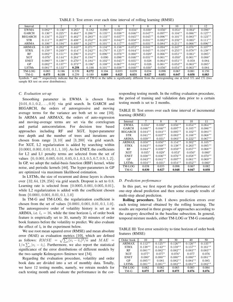
TABLE I: Test errors over each time interval of rolling learning (RMSE)
Interval 1 2 3 4 5 6 7 8 9 10 11 12
EWMA 0.082∗∗ 0.136∗ 0.265∗ 0.182 0.096∗ 0.027∗ 0.034∗ 0.030∗ 0.056∗ 0.054∗ 0.064∗ 0.096∗
GARCH 0.136∗∗ 0.225∗∗ 0.464∗∗ 0.286∗∗ 0.135∗∗ 0.038∗∗ 0.046∗∗ 0.047∗∗ 0.097∗∗ 0.104∗∗ 0.086∗∗ 0.127∗∗
BEGARCH 0.134∗∗ 0.223∗∗ 0.462∗∗ 0.283∗∗ 0.133∗∗ 0.037∗∗ 0.045∗∗ 0.045∗∗ 0.096∗∗ 0.101∗∗ 0.083∗∗ 0.123∗∗
STR 0.111∗∗ 0.207∗∗ 0.408∗∗ 0.252∗∗ 0.105∗∗ 0.042∗∗ 0.058∗∗ 0.031∗∗ 0.082∗∗ 0.232∗∗ 0.065∗ 0.111∗∗
ARIMA 0.106∗∗ 0.194∗∗ 0.409∗∗ 0.247∗∗ 0.101∗∗ 0.117∗∗ 0.037∗∗ 0.031∗∗ 0.084∗∗ 0.211∗∗ 0.066∗∗ 0.096∗∗
ARIMAX 0.126∗∗ 0.282∗∗ 0.443∗∗ 0.271∗∗ 0.134∗∗ 0.156∗∗ 0.072∗∗ 0.041∗∗ 0.094∗∗ 0.247∗∗ 0.076∗∗ 0.107∗∗
STRX 0.159∗∗ 0.249∗∗ 0.414∗∗ 0.242∗∗ 0.176∗∗ 0.125∗∗ 0.044∗∗ 0.045∗∗ 0.104∗∗ 0.255∗∗ 0.078∗∗ 0.138∗∗
RF 0.082∗∗ 0.151∗∗ 0.296∗∗ 0.212∗∗ 0.096∗∗ 0.076∗∗ 0.060∗∗ 0.029∗ 0.066∗∗ 0.051∗∗ 0.061∗ 0.085∗
XGT 0.076∗ 0.144∗∗ 0.264∗∗ 0.194∗∗ 0.090 0.096∗∗ 0.046∗∗ 0.031∗∗ 0.061∗∗ 0.050∗ 0.061∗∗ 0.088∗
ENET 0.080∗∗ 0.138∗∗ 0.270∗∗ 0.184∗∗ 0.102∗∗ 0.045∗∗ 0.035∗∗ 0.028 0.064∗∗ 0.051∗∗ 0.059 0.084
GP 0.082∗∗ 0.137∗∗ 0.373∗∗ 0.196∗ 0.108∗∗ 0.067∗∗ 0.042∗∗ 0.028 0.061∗∗ 0.053∗∗ 0.063∗∗ 0.085∗
LSTMs 0.081∗∗ 0.133∗∗ 0.258 0.190 0.101∗∗ 0.038∗∗ 0.040∗∗ 0.030∗ 0.056∗ 0.054∗∗ 0.063∗∗ 0.084
TM-LOG 0.083 0.186 0.339 0.172 0.104 0.033 0.039 0.034 0.098 0.067 0.081 0.150TM-G 0.075 0.118 0.259 0.189 0.089 0.025 0.031 0.027 0.051 0.047 0.058 0.083
Symbols * and ** respectively indicate that the error of TM-G in the table is significantly different from the corresponding one at level 5% and 1% (twosample KS test on error distributions).
C. Evaluation set-up
Smoothing parameter in EWMA is chosen from
{0.01, 0.1, 0.2, . . . , 0.9} via grid search. In GARCH and
BEGARCH, the orders of autoregressive and moving
average terms for the variance are both set to one [10].
In ARIMA and ARIMAX, the orders of auto-regression
and moving-average terms are set via the correlogram
and partial autocorrelation. For decision tree based
approaches including RF and XGT, hyper-parameter
tree depth and the number of trees and iterations are
chosen from range [3, 10] and [3, 200] via grid search.
For XGT, L2 regularization is added by searching within
{0.0001, 0.001, 0.01, 0.1, 1, 10}. As for ENET, the coefficients
for L2 and L1 penalty terms are selected from the set of
values {0, 0.001, 0.005, 0.01, 0.05, 0.1, 0.3, 0.5, 0.7, 0.9, 1, 2}.
In GP, we adopt the radial-basis function (RBF) kernel, white
noise, and periodic kernels [44]. The hyper-parameters in GP
are optimized via maximum likelihood estimation.
In LSTMs, the size of recurrent and dense layers is chosen
over {32, 64, 128, 256} via grid search. Dropout is set to 0.8.
Learning rate is selected from {0.0005, 0.001, 0.005, 0.01},
while L2 regularization is added with the coefficient chosen
from {0.0001, 0.001, 0.01, 0.1, 1.0}In TM-G and TM-LOG, the regularization coefficient is
chosen from the set of values {0.0001, 0.001, 0.01, 0.1, 1.0}.
The autoregressive order of volatility history is set as in
ARIMA, i.e. lv = 16, while the time horizon lb of order book
feature is empirically set to 30, namely 30 minutes of order
book features before the volatility to predict. We also evaluate
the effect of lb in the experiment below.
We use root mean squared error (RMSE) and mean absolute
error (MAE) as evaluation metrics [10], which are defined
as follows: RMSE =√∑
i(vi − vi)2/n and MAE =1/n
∑
i |vi − vi|. Furthermore, we also report the statistical
significance of the error distributions of different models by
the two-sample Kolmogorov-Smirnov test [34].
Regarding the evaluation procedure, volatility and order
book data are divided into a set of monthly data. Totally,
we have 12 testing months, namely, we retrain models for
each testing month and evaluate the performance in the cor-
responding testing month. In the rolling evaluation procedure,
the period of training and validation data prior to a certain
testing month is set to 3 months.
TABLE II: Test errors over each time interval of incremental
learning (RMSE)
Internal 7 8 9 10 11
EWMA 0.034∗ 0.030∗ 0.056∗∗ 0.054∗∗ 0.064∗∗
GARCH 0.046∗∗ 0.046∗∗ 0.097∗∗ 0.105∗∗ 0.086∗∗
BEGARCH 0.044∗∗ 0.044∗∗ 0.095∗∗ 0.102∗∗ 0.084∗∗
STR 0.041∗∗ 0.037∗∗ 0.083∗∗ 0.188∗∗ 0.068∗∗
ARIMA 0.039∗∗ 0.031∗ 0.083∗∗ 0.222∗∗ 0.067∗∗
ARIMAX 0.058∗∗ 0.050∗∗ 0.154∗∗ 0.302∗∗ 0.105∗∗
STRX 0.043∗∗ 0.048∗∗ 0.138∗∗ 0.263∗∗ 0.095∗∗
RF 0.044∗∗ 0.039∗∗ 0.059∗∗ 0.057∗∗ 0.068∗∗
XGT 0.035∗ 0.029∗ 0.053∗ 0.050∗ 0.060∗
ENET 0.038∗∗ 0.036∗∗ 0.076∗∗ 0.058∗∗ 0.070∗∗
GP 0.043∗∗ 0.041∗∗ 0.097∗∗ 0.061∗∗ 0.069∗∗
LSTMs 0.034∗∗ 0.031∗ 0.054∗∗ 0.052∗∗ 0.060∗
TM-LOG 0.038 0.033 0.098 0.067 0.082TM-G 0.030 0.027 0.048 0.047 0.058
D. Prediction performance
In this part, we first report the prediction performance of
one-step ahead prediction and then some example results of
multi-step ahead prediction.
Rolling procedure. Tab. I shows prediction errors over
each testing interval obtained by the rolling learning. The
results are reported in three groups of approaches according to
the category described in the baseline subsection. In general,
temporal mixture models, either TM-LOG or TM-G constantly
TABLE III: Test error sensitivity to time horizon of order book
features (RMSE)
Order book 10 20 30 40 50
ARIMAX 0.112∗∗ 0.125∗∗ 0.126∗∗ 0.126∗∗ 0.135∗∗
STRX 0.138∗∗ 0.142∗∗ 0.159∗∗ 0.157∗∗ 0.161∗∗
RF 0.081∗∗ 0.082∗∗ 0.082∗∗ 0.083∗∗ 0.083∗∗
XGT 0.077∗ 0.077∗ 0.076∗ 0.077 0.076
ENET 0.080∗ 0.080∗∗ 0.080∗∗ 0.080∗∗ 0.081∗∗
GP 0.095∗∗ 0.081 0.082∗∗ 0.084∗∗ 0.085
LSTMs 0.081∗∗ 0.081∗∗ 0.082∗∗ 0.081∗∗ 0.082∗∗
TM-LOG 0.082 0.082 0.083 0.083 0.084TM-G 0.075 0.075 0.075 0.076 0.076

0 20 40 60 80 100
Tim e offs e t [hour]
0
1
2
3
4
5
Vo
lati
lity
00:00AM, June , 20th, 2016Truth
Prediction
0 20 40 60 80 100
Tim e offs e t [hour]
0
1
2
3
4
5
Vo
lati
lity
08:00PM, July, 15th, 2016Truth
Prediction
0 20 40 60 80 100
Tim e offs e t [hour]
0
1
2
3
4
5
Vo
lati
lity
08:00PM, Dec., 17th, 2016Truth
Prediction
0 20 40 60 80 100
Tim e offs e t [hour]
0.0
0.2
0.4
0.6
0.8
1.0
Ga
te v
alu
e
0 20 40 60 80 100
Tim e offs e t [hour]
0.0
0.2
0.4
0.6
0.8
1.0
Ga
te v
alu
e
0 20 40 60 80 100
Tim e offs e t [hour]
0.0
0.2
0.4
0.6
0.8
1.0
Ga
te v
alu
e
0 20 40 60 80 100
Tim e offs e t [hour]
0
2
4
6
8
10
Sp
re
ad
0 20 40 60 80 100
Tim e offs e t [hour]
0
100
200
300
400
500
As
k s
lop
e
0 20 40 60 80 100
Tim e offs e t [hour]
0
100
200
300
400
500
As
k s
lop
e0 20 40 60 80 100
Tim e offs e t [hour] (a)
1000
500
0
500
1000
De
pth
dif
f.
0 20 40 60 80 100
Tim e offs e t [hour] (b )
0
100
200
300
400
500
Bid
slo
pe
0 20 40 60 80 100
Tim e offs e t [hour] (c)
0
100
200
300
400
500
Bid
slo
pe
Fig. 5: Temporal Mixture model visualization. Each column of figures represents the results from the mixture model on a
sample testing period, where the time offset is measured in hours w.r.t. to (a) 00:00AM, June, 20th, 2016, (b) 08:00PM, July,
15th, 2016 and (c) 08:00PM, December, 17th, 2016. Top panel: prediction and true values of three sample periods. Second
panel: mixture gate value gh (in yellow color for the weight of volatility history) and 1− gh (in gray color for the weight of
order book component model) over time. Bottom two panels: order book feature values over time. (Best viewed in color.)
TABLE IV: Test errors of 5-step ahead prediction (RMSE)
Interval 7 8 9 10 11
EWMA 0.036 0.035∗ 0.077∗∗ 0.069∗∗ 0.067∗
GARCH 0.049∗∗ 0.046∗∗ 0.101∗∗ 0.111∗∗ 0.089∗∗
BEGARCH 0.048∗∗ 0.044∗∗ 0.103∗∗ 0.107∗∗ 0.087∗∗
STR 0.051∗∗ 0.037∗∗ 0.088∗∗ 0.194∗∗ 0.069∗∗
ARIMA 0.049∗∗ 0.033∗ 0.089∗∗ 0.232∗∗ 0.071∗∗
ARIMAX 0.062∗∗ 0.050∗∗ 0.161∗∗ 0.303∗∗ 0.109∗∗
STRX 0.049∗∗ 0.048∗∗ 0.142∗∗ 0.268∗∗ 0.098∗∗
RF 0.040∗∗ 0.033 0.075∗∗ 0.060∗∗ 0.067
XGT 0.058∗ 0.033 0.068∗ 0.063∗ 0.069∗
ENET 0.039∗∗ 0.033 0.079∗∗ 0.057∗ 0.067∗
GP 0.048∗∗ 0.049∗∗ 0.101∗∗ 0.061∗∗ 0.069∗
LSTMs 0.046∗∗ 0.033 0.075∗∗ 0.068∗∗ 0.072∗∗
TM-LOG 0.039 0.038 0.101 0.069 0.095TM-G 0.035 0.032 0.064 0.054 0.065
outperform others. Basically, approaches using both volatility
and order book features perform better than those using only
volatility or return series, however, the simple EWMA can beat
many others except for temporal mixture models and LSTMs
in some intervals. Particularly, in the middle group of Tab. I,
ARIMAX and STRX using both volatility and order book data
fail to outperform their counterparts, i.e. ARIMA and STR in
the top group. It suggests that simply adding features from
order book does not necessarily improve the performance.
Ensemble and regularized regression perform better, e.g. XGT
and ENET perform the best in most of the cases, within this
group.
Gaussian temporal mixture, i.e. TM-G model outperforms
other approaches in most of the cases. Specifically, it can
achieve 50% less errors at most. LSTMs has comparable
performance as TM-G in some intervals. Although the volatil-
ity lies only on non-negative range of values, surprisingly
TM-LOG is still inferior to TM-G. One possible explana-
tion is that on the short time scales the random variables
vh | {v[h ,−lv] , zh = 0} and vh | {X[i(h) ,−lb] , zh = 1} are
better explained with the Gaussian since the variations in short
time scale cannot lead to the heavy-tail of the log-normal
distribution.
Incremental procedure. Tab. II shows the prediction errors

obtained by the incremental procedure. By comparing the
errors in Tab. II and Tab. I w.r.t. a certain model and interval,
we study the robustness of each model. The errors in the front
few intervals are comparable to the ones in Tab. I, because
the look-back horizon of training data in the incremental
procedure is wider than that in the rolling procedure and
the growing size of training data benefits the model training.
However, when the horizon further increases, it is interesting
to find that such trend changes. Due to the page limitation, we
list the results from interval 7 to 11 in Tab. II.
For the models in the top group which do not ingest order
book features, the errors of EWMA, GARCH, BEGARCH,
and STR are close to the corresponding ones in Tab. I,
though for ARIMA, the errors in interval 10 and 11 present
little ascending pattern. In the middle group, models except
LSTMs exhibit decreasing and then increasing error pattern,
compared with their counterparts in Tab. I. This suggests
that too old data in the training set begins to deteriorate
the prediction performance instead. LSTMs presents robust
performance because of the gate and memory mechanism, i.e.
errors are comparable over all intervals in Tab. II and Tab.
I. Due to the adaptive weighting mechanism over order book
features, TM-G and TM-LOG are robust to increasing amount
of training data as well. Above observations in Tab. I and Tab.
II apply to MAE results below as well.
Time horizon of order book feature. Tab. III demonstrates
the effect of time horizon (i.e. lb) of order book features on
the prediction performance of models using order book. The
results are obtained by evaluating each model on the interval 1with increasing size of lb. It exhibits that short-term order book
features are sufficient for most of the models and furthermore
data, e.g. 40 and 50 minutes of order book features, leads to no
improvement. In particular, models like ARIMAX and STRX
are prone to overfit by redundant data of long horizon, while
our mixture models, LSTMs, XGT, and ENET are relatively
insensitive to the horizon.
Multi-step ahead prediction. In Tab. IV, we demonstrate
the performance of multi-step-ahead prediction by example
results of 5-step ahead prediction obtained by the rolling
procedure. Full results will be presented in the future work due
to the page limitation. Basically, in 5-step ahead prediction
all the models present higher errors in comparison to one
step ahead prediction in Tab. I. TM-G constantly outperforms
baselines.
E. Model interpretation
In this part, we provide insights into the data by analyzing
the components of the model. Specifically, in Fig. 5 each
column of figures corresponds to a sample period from the
testing month. The top panel shows the model prediction and
true values of the period. The second panel demonstrates the
distribution of gate values in the mixture model corresponding
to the top panel. The dark area corresponds to the gate values
1 − gh of the component model w.r.t. the order book at each
time step. The sum of dark and light areas at each time step
is equal to one and therefore the lower the dark area reaches,
the higher gate value is assigned to the component model of
the order book. The time evolution of the inferred gate values
gh and 1 − gh in our mixture model explains the dynamical
importance and interplay of the order book features for high
volatility regimes. Thus, it implies that the order book features
can encode the future short-term price fluctuations from the
trade orders.
The bottom two panels exhibit two order book features
with high coefficients in the mixture model. It demonstrates
the correspondence between feature and gate values over
time. Recall that each hourly volatility observation has the
associated order book features over a time horizon lb and
therefore the value range within lb of each feature at each hour
is shown in the figures. If we look at column (a) the large
price fluctuations at the offset of 20 hours from 2016 June,
20th, 00:00 am are mostly driven by the negative market depth
feature (panel four) which implies larger buying demand for
the Bitcoins coupled together with the larger spread between
bid and ask price (panel three). Similarly, the large volatility
around the offset of 40 hours from 2016 July, 15th, 08:00 pm
in panel (b) is driven by the large bid slope i.e. buying demand
near the currently traded price w.r.t. much smaller ask slope
i.e. selling offer near the current traded price. In contrast, in
panel (c) at the offset of around 60 hours from 2016 December,
17th, 08:00 pm the medium price fluctuations are driven by
larger selling offer near the current traded price. These three
cases show the interpretability of the dynamical effects in our
temporal mixture model to learn the future short-term volatility
from the order book.
VII. CONCLUSION
In this paper, we study the short-term volatility of Bitcoin
market by realized volatility observations and order book
snapshots. We propose temporal mixture models to capture
the dynamical effect of order book features on the volatility
evolution for improved prediction and interpretable results.
We performed comprehensive experiments to compare with
numerous statistical and machine learning baselines. The pro-
posed temporal mixture models have four favorable properties
as: (i) it is more accurate in most of the cases than the
conventional way of learning data from different sources,
which trains models on fused features or learns joint features
for prediction. (ii) by visualizing the mixture gate values and
important features over time, it enables to interpret the effect
of order book on the volatility. (iii) by comparing the pre-
diction performance under rolling and incremental evaluation
procedures, we found out that our temporal mixture model is
robust and adaptive w.r.t. time-varying data. (iv) it can also
serve as a flexible and generic framework for Bitcoin data
forecasting and interpretation by adding component models
specific to different data sources.
ACKNOWLEDGEMENT
The work of T.G. and N.A.-F. has been funded by the EU
Horizon 2020 SoBigData project under grant agreement No.
654024.

TABLE V: Test errors over each time interval of rolling learning (MAE)
Interval 1 2 3 4 5 6 7 8 9 10 11 12
EWMA 0.047 0.063 0.158∗ 0.075∗ 0.050 0.018∗∗ 0.018 0.019∗ 0.026∗ 0.030∗ 0.032∗ 0.040∗
GARCH 0.099∗∗ 0.133∗∗ 0.333∗∗ 0.147∗∗ 0.091∗∗ 0.019∗∗ 0.029∗∗ 0.035∗∗ 0.054∗∗ 0.075∗∗ 0.057∗∗ 0.084∗∗
BEGARCH 0.096∗∗ 0.131∗∗ 0.330∗∗ 0.142∗∗ 0.087∗∗ 0.016∗ 0.027∗∗ 0.033∗∗ 0.052∗∗ 0.071∗∗ 0.053∗∗ 0.079∗∗
STR 0.065∗∗ 0.105∗∗ 0.254∗∗ 0.141∗∗ 0.051 0.028∗∗ 0.040∗∗ 0.022∗∗ 0.036∗∗ 0.220∗∗ 0.034∗ 0.065∗∗
ARIMA 0.059∗∗ 0.091∗∗ 0.255∗∗ 0.123∗∗ 0.053∗ 0.045∗∗ 0.020∗∗ 0.022∗∗ 0.037∗∗ 0.204∗∗ 0.032∗∗ 0.051∗∗
ARIMAX 0.083∗∗ 0.172∗∗ 0.295∗∗ 0.140∗∗ 0.092∗∗ 0.050∗∗ 0.027∗∗ 0.030∗∗ 0.045∗∗ 0.236∗∗ 0.042∗∗ 0.062∗∗
STRX 0.103∗∗ 0.152∗∗ 0.219∗∗ 0.163∗∗ 0.105∗∗ 0.038∗∗ 0.047∗∗ 0.023∗∗ 0.051∗∗ 0.175∗∗ 0.403∗∗ 0.063∗∗
RF 0.052∗∗ 0.089∗∗ 0.174∗∗ 0.095∗∗ 0.060∗∗ 0.071∗∗ 0.031∗∗ 0.018 0.031∗∗ 0.031∗∗ 0.037∗∗ 0.040∗
XGT 0.047∗ 0.077∗∗ 0.159∗∗ 0.080 0.057∗∗ 0.051∗∗ 0.031∗∗ 0.020∗∗ 0.029∗∗ 0.031∗∗ 0.034∗∗ 0.041∗
ENET 0.052∗∗ 0.074∗∗ 0.166∗∗ 0.093∗∗ 0.064∗∗ 0.036∗∗ 0.024∗∗ 0.017 0.028∗∗ 0.030∗∗ 0.032∗∗ 0.035∗
GP 0.050∗∗ 0.070∗∗ 0.216∗∗ 0.084∗ 0.069∗∗ 0.055∗∗ 0.025∗∗ 0.018 0.028∗∗ 0.034∗∗ 0.037∗∗ 0.035∗
LSTMs 0.048∗ 0.073∗∗ 0.154 0.084∗ 0.059∗∗ 0.022∗∗ 0.030∗∗ 0.022∗ 0.030∗∗ 0.032∗∗ 0.031∗ 0.036∗
TM-LOG 0.053 0.078 0.176 0.070 0.061 0.018 0.024 0.041 0.037 0.037 0.103 0.053TM-G 0.044 0.063 0.153 0.079 0.050 0.014 0.017 0.017 0.024 0.026 0.029 0.032
.
TABLE VI: Test errors over each time interval of incremental
learning (MAE)
Interval 7 8 9 10 11
EWMA 0.018 0.019∗ 0.026∗ 0.030∗ 0.032∗
GARCH 0.028∗∗ 0.035∗∗ 0.054∗∗ 0.075∗∗ 0.057∗
BEGARCH 0.025∗∗ 0.032∗∗ 0.051∗∗ 0.071∗∗ 0.053∗
STR 0.022∗ 0.030∗∗ 0.037∗∗ 0.179∗∗ 0.032∗
ARIMA 0.020∗ 0.021∗ 0.037∗∗ 0.215∗∗ 0.032∗
ARIMAX 0.037∗∗ 0.037∗∗ 0.078∗∗ 0.291∗∗ 0.064∗∗
STRX 0.048∗∗ 0.043∗∗ 0.064∗∗ 0.195∗∗ 0.077∗∗
RF 0.034∗∗ 0.031∗∗ 0.039∗∗ 0.041∗∗ 0.048∗∗
XGT 0.023∗∗ 0.021∗ 0.032∗∗ 0.030∗ 0.032∗
ENET 0.026∗∗ 0.025∗∗ 0.041∗∗ 0.038∗∗ 0.052∗∗
GP 0.028∗∗ 0.028∗∗ 0.050∗∗ 0.039∗∗ 0.040∗
LSTMs 0.025∗∗ 0.023∗∗ 0.029∗∗ 0.033∗∗ 0.032∗
TM-LOG 0.025 0.039 0.038 0.037 0.104TM-G 0.017 0.017 0.024 0.027 0.030
REFERENCES
[1] S. Nakamoto, “Bitcoin: A peer-to-peer electronic cash system,” 2008.[Online]. Available: http://bitcoin.org/bitcoin.pdf
[2] R. Næs and J. A. Skjeltorp, “Order book characteristics and the vol-ume–volatility relation: Empirical evidence from a limit order market,”Journal of Financial Markets, vol. 9, pp. 408–432, 2006.
[3] J. Chu, S. Nadarajah, and S. Chan, “Statistical analysis of the exchangerate of bitcoin,” PLOS ONE, vol. 10, no. 7, pp. 1–27, 2015.
[4] E.-T. Cheah and J. Fry, “Speculative bubbles in bitcoin markets? an em-pirical investigation into the fundamental value of bitcoin,” Economics
Letters, vol. 130, pp. 32–36, 2015.
[5] D. Garcia, C. J. Tessone, P. Mavrodiev, and N. Perony, “The digitaltraces of bubbles: feedback cycles between socio-economic signals inthe bitcoin economy,” Journal of The Royal Society Interface, vol. 11,no. 99, pp. 20 140 623–20 140 623, 2014.
[6] J. Donier and J.-P. Bouchaud, “Why do markets crash? bitcoin dataoffers unprecedented insights,” PLOS ONE, vol. 10, pp. 1–11, 2015.
[7] L. Kristoufek, “Bitcoin meets google trends and wikipedia: Quantifyingthe relationship between phenomena of the internet era,” Scientific
reports, vol. 3, p. 3415, 2013.
[8] L. a. Kristoufek, “What are the main drivers of the bitcoin price?evidence from wavelet coherence analysis,” PloS one, vol. 10, no. 4,p. e0123923, 2015.
[9] T. G. Andersen, T. Bollerslev, F. X. Diebold, and P. Labys, “Modelingand forecasting realized volatility,” Econometrica, vol. 71, pp. 579–625,2003.
[10] P. R. Hansen and A. Lunde, “A forecast comparison of volatility models:does anything beat a GARCH(1, 1)?” Journal of Applied Econometrics,vol. 20, pp. 873–889, 2005.
[11] J. Fleming, C. Kirby, and B. Ostdiek, “The economic value of volatilitytiming using “realized” volatility,” Journal of Financial Economics,vol. 67, pp. 473–509, 2003.
[12] M. Piskorec, N. Antulov-Fantulin, P. K. Novak, I. Mozetic, M. Grcar,I. Vodenska, and T. Smuc, “Cohesiveness in financial news and itsrelation to market volatility,” Scientific Reports, vol. 4, 2014.
[13] M. D. Gould, M. A. Porter, S. Williams, M. McDonald, D. J. Fenn,and S. D. Howison, “Limit order books,” Quantitative Finance, vol. 13,no. 11, pp. 1709–1742, 2013.
[14] H. Jang and J. Lee, “An empirical study on modeling and predictionof bitcoin prices with bayesian neural networks based on blockchaininformation,” IEEE Access, vol. 6, pp. 5427–5437, 2018.
[15] Y. B. Kim, J. G. Kim, W. Kim, J. H. Im, T. H. Kim, S. J. Kang, andC. H. Kim, “Predicting fluctuations in cryptocurrency transactions basedon user comments and replies,” PloS one, vol. 11, 2016.
[16] M. Amjad and D. Shah, “Trading bitcoin and online time seriesprediction,” in NIPS 2016 Time Series Workshop, 2017, pp. 1–15.
[17] L. Alessandretti, A. ElBahrawy, L. M. Aiello, and A. Baronchelli,“Machine learning the cryptocurrency market,” arXiv preprint
arXiv:1805.08550, 2018.
[18] T. R. Li, A. S. Chamrajnagar, X. R. Fong, N. R. Rizik, andF. Fu, “Sentiment-based prediction of alternative cryptocurrency pricefluctuations using gradient boosting tree model,” arXiv preprint
arXiv:1805.00558, 2018.
[19] P. Katsiampa, “Volatility estimation for bitcoin: A comparison ofGARCH models,” Economics Letters, vol. 158, pp. 3–6, 2017.
[20] L. Zhang, C. Aggarwal, and G.-J. Qi, “Stock price prediction viadiscovering multi-frequency trading patterns,” in SIGKDD. ACM, 2017,pp. 2141–2149.
[21] A. M. Rather, A. Agarwal, and V. Sastry, “Recurrent neural networkand a hybrid model for prediction of stock returns,” Expert Systems
with Applications, vol. 42, pp. 3234–3241, 2015.
[22] Y. Jiao and J. Jakubowicz, “Predicting stock movement direction withmachine learning: An extensive study on s&p 500 stocks,” in Big Data
(Big Data), 2017 IEEE International Conference on. IEEE, 2017, pp.4705–4713.
[23] J. Y. Campbell and S. B. Thompson, “Predicting excess stock returnsout of sample: Can anything beat the historical average?” The Review
of Financial Studies, vol. 21, no. 4, pp. 1509–1531, 2007.
[24] J. Si, A. Mukherjee, B. Liu, Q. Li, H. Li, and X. Deng, “Exploiting topicbased twitter sentiment for stock prediction,” in Proceedings of the 51st
Annual Meeting of the Association for Computational Linguistics, vol. 2,2013, pp. 24–29.
[25] Z. Hu, W. Liu, J. Bian, X. Liu, and T.-Y. Liu, “Listening to chaoticwhispers: A deep learning framework for news-oriented stock trendprediction,” arXiv preprint arXiv:1712.02136, 2017.
[26] X. Ding, Y. Zhang, T. Liu, and J. Duan, “Deep learning for event-drivenstock prediction.” in IJCAI, 2015, pp. 2327–2333.
[27] T. H. Nguyen and K. Shirai, “Topic modeling based sentiment analysison social media for stock market prediction,” in Proceedings of the 53rd
Annual Meeting of the Association for Computational Linguistics, vol. 1,2015, pp. 1354–1364.
[28] Y. Xu and S. B. Cohen, “Stock movement prediction from tweets andhistorical prices,” in Proceedings of the 2014 Conference on Empirical
Methods in Natural Language Processing (EMNLP), 2018.
[29] M. Oyamada and S. Nakadai, “Relational mixture of experts: Explain-able demographics prediction with behavioral data,” in 2017 IEEE

International Conference on Data Mining (ICDM). IEEE, 2017, pp.357–366.
[30] M. I. Jordan and R. A. Jacobs, “Hierarchical mixtures of experts andthe em algorithm,” Neural computation, vol. 6, pp. 181–214, 1994.
[31] S. E. Yuksel, J. N. Wilson, and P. D. Gader, “Twenty years of mixture ofexperts,” IEEE transactions on neural networks and learning systems,vol. 23, pp. 1177–1193, 2012.
[32] X. Wei, J. Sun, and X. Wang, “Dynamic mixture models for multipletime-series.” in IJCAI, vol. 7, 2007, pp. 2909–2914.
[33] R. J. Hyndman and G. Athanasopoulos, Forecasting: principles and
practice. OTexts, 2014.[34] K. P. Murphy, Machine learning: a probabilistic perspective. MIT
press, 2012.[35] J. V. Shi, Y. Xu, and R. G. Baraniuk, “Sparse bilinear logistic regres-
sion,” arXiv preprint arXiv:1404.4104, 2014.[36] B. Hooi, S. Liu, A. Smailagic, and C. Faloutsos, “Beatlex: Summarizing
and forecasting time series with patterns,” in ECML/PKDD. Springer,2017, pp. 3–19.
[37] N. Laptev, J. Yosinski, L. E. Li, and S. Smyl, “Time-series extremeevent forecasting with neural networks at uber,” in ICML, 2017.
[38] G. Kirchgassner and J. Wolters, Introduction to modern time series
analysis. Springer Science & Business Media, 2007.[39] S. L. Scott and H. R. Varian, “Predicting the present with bayesian
structural time series,” International Journal of Mathematical Modelling
and Numerical Optimisation, vol. 5, pp. 4–23, 2014.[40] A. C. Harvey and T. Chakravarty, “Beta-t-(e) garch,” 2008.[41] A. Liaw, M. Wiener et al., “Classification and regression by randomfor-
est,” R news, vol. 2, pp. 18–22, 2002.[42] T. Chen and C. Guestrin, “Xgboost: A scalable tree boosting system,”
in SIGKDD. ACM, 2016, pp. 785–794.[43] Y. Liu, A. Niculescu-Mizil, A. C. Lozano, and Y. Lu, “Learning temporal
causal graphs for relational time-series analysis,” in ICML, 2010, pp.687–694.
[44] S. Brahim-Belhouari and A. Bermak, “Gaussian process for nonstation-ary time series prediction,” Computational Statistics & Data Analysis,vol. 47, pp. 705–712, 2004.
[45] Y. Wu, J. M. Hernandez-Lobato, and Z. Ghahramani, “Gaussian processvolatility model,” in NIPS, 2014, pp. 1044–1052.
[46] T. Guo and T. Lin, “Multi-variable lstm neural network for autoregres-sive exogenous model,” arXiv preprint arXiv:1806.06384, 2018.
[47] T. Guo, T. Lin, and Y. Lu, “An interpretable lstm neural network forautoregressive exogenous model,” in workshop track at International
Conference on Learning Representations, 2018.[48] Y. Qin, D. Song, H. Cheng, W. Cheng, G. Jiang, and G. W. Cottrell,
“A dual-stage attention-based recurrent neural network for time seriesprediction,” in IJCAI’17. AAAI Press, 2017, pp. 2627–2633.