bitcoin price prediction based on other cryptocurrencies
TRANSCRIPT
1
Bitcoin Price Prediction Based on Other Cryptocurrencies Using Machine Learning and
Time Series Analysis
Negar Malekia, Alireza Nikoubina, Masoud Rabbania,, Yasser Zeinalib
a. School of Industrial Engineering, College of Engineering, University of Tehran, P.O. Box: 11155-
4563, Tehran, Iran.
b. School of Industrial Engineering, Sharif University of Technology, Tehran, Iran.
Abstract
Cryptocurrencies, which the Bitcoin is the most remarkable one, have allured substantial
awareness up to now, and they have encountered enormous instability in their price. While some
studies utilize conventional statistical and econometric ways to uncover the driving variables of
Bitcoin's prices, experimentation on the advancement of predicting models to be used as decision
support tools in investment techniques is rare. There are many different predicting
cryptocurrencies' price methods that cover various purposes, such as forecasting a one-step
approach that can be done through time series analysis, neural networks, and machine learning
algorithms. Sometimes realizing the trend of a coin in a long run period is needed. In this paper,
some machine learning algorithms are applied to find the best ones that can forecast Bitcoin price
based on three other famous coins. Second, a new methodology is developed to predict Bitcoin's
worth, this is also done by considering different cryptocurrencies prices (Ethereum, Zcash, and
Litecoin). The results demonstrated that Zcash has the best performance in forecasting Bitcoin's
price without any data on Bitcoin's fluctuations price among these three cryptocurrencies.
Keywords: Cointegration, Time Series Models, Machine Learning, Bitcoin, Price Prediction
1. Introduction
Time series prediction can be used in different areas, such as predicting climate changes,
population variations, the demand for any staff, and financial markets [1]. Economic time series is
one of the most exciting and practical branches which can give a brilliant insight into financial
markets. There are many different financial time series data, such as stocks and bond prices, energy
prices, etc. Time series models, other processes, and their changes can be tracked to recognize
what has happened and what will happen in the future. In financial fields, many various digital
currencies are having been analyzed through different aspects.
A cryptocurrency is an advanced resource intended to function as a trade mechanism that
utilizes solid cryptography to verify monetary exchanges; every unit of it can be controlled through
different applications. Cryptographic forms of money use decentralized control rather than
incorporated computerized cash and focal financial systems [2]. The decentralized control of every
digital currency works through circulated record innovation, ordinarily, a blockchain, that fills in
as an open budgetary exchange database. Bitcoin, first discharged as open-source programming in
Corresponding author
Tel.: +9821 88350642
Fax: +9821 88350642
E-mail addresses: [email protected] (N. Maleki): +989128934891, [email protected] (A. Nikoubin):
+989375610269, [email protected] (M. Rabbani): +989121403975, [email protected] (Y. Zeinali):
+989013075085
2
2009, is commonly viewed as the principal decentralized digital money. Since Bitcoin's arrival,
more than 4,000 different digital currencies have been made, such as Ethereum, Litecoin, Zcash,
etc. Bitcoin has become one of the most popular assets in the cryptocurrency market. Unlike
traditional credit currencies, Bitcoin allows people to transfer money or purchase commodities via
a peer-to-peer payment network without a centralized regulatory body [3].
Cryptocurrencies have means, variances, and covariances that change over time, which is
called non-stationary. Non-stationary behaviors can be random walks, trends, cycles, or
combinations of the three. Non-stationary data are unpredictable and cannot be modeled or
forecasted [4]. The results obtained by using non-stationary time series may be spurious in that
they may indicate a relationship between two variables where one does not exist. The non-
stationary data needs to be transformed into stationary data to receive reliable results. In contrast
to the non-stationary process with a variable variance and a mean that does not remain near, or
returns to a long-run mean over time, the stationary process reverts around a constant long-term
mean and has a constant variance independent of time. Using non-stationary time series data
produces unreliable and spurious results and leads to poor understanding and forecasting in
financial models. The solution to the problem is to transform the time series data so that it becomes
stationary [5].
There are a few sorts of motivation for time series which are fitting for various purposes.
For example curve fitting, is the way toward developing a curve, or mathematical function that has
the best fit to a series of information focuses [6], function approximation, choose a function among
a very much characterized class that intently coordinates ("approximates") an objective function
in an errand explicit manner, prediction, and forecasting, etc. Prediction and forecasting in time
series are developed by various models like Autoregressive (AR), Moving Average (MA),
Autoregressive Moving Average (ARMA), Autoregressive Integrated Moving Average (ARIMA),
Autoregressive Conditional Heteroskedasticity (ARCH), Generalized Autoregressive Conditional
Heteroskedasticity (GARCH), Adaptive Neuro-Fuzzy Inference System (ANFIS), and Artificial
Neural Networks (ANN) are used as artificial intelligence models for analyzing the time series
data.
This paper's main contribution is around forecasting the price of cryptocurrencies using a
new approach based on the cointegration of different currencies to make them stationary for being
predictable and determine the best coordination of cryptocurrencies. Analyzing the cointegration
has two steps; first, we regress the dependent variable on the independent variable. The statistical
tests should be run on equations to test null-hypothesis that is the condition in which both
currencies are cointegrated. Following the first contribution, the second one estimates the best lag
of models based on different performance criteria.
The rest of this paper is organized as follows. Section 2 reviews different estimating models
of digital currency time series found in the literature. Section 3 exhibits the outline of what is done
in this study and its methods to make them clear and understandable. Section 4 depicts the
recommended approaches and their scenarios in foreseeing prices. The best empirical construction
demonstrates in Section 5. The study is concluded, and the outcomes of the suggested model and
other instability foreseeing models are introduced and discussed in Section 6. Finally, future work
was presented.
3
2. Literature Review
Autoregressive Integrated Moving Average (ARIMA) and lagged forward price modeling
were used to forecast the price of lead and zinc prices. Dooley and Lenihan [7] have indicated that
both methods can be useful for price prediction in mine industries. Concerning zinc, there was no
definitive proof to propose that one model was better than the other in its forecasting ability. On
account of lead, it was discovered that the ARIMA model works better. In this investigation, Ediger
and Akar [8] used the ARIMA and regular ARIMA (SARIMA) techniques to assess Turkey's
future essential energy demand request from 2005 to 2020. Khashei and Bijari [9] utilized a hybrid
methodology that combines ANN and ARIMA for forecasting time series. They have compared
their model to different methods such as ARIMA, ANN, and Zhang's hybrid model, and they
achieved better performance. Their model's mean Square Error (MSE) was considerably smaller
than utilizing only the Artificial Neural Networks (ANN) or ARIMA models in prediction. Their
forecast horizon was 1, 6, 12 months, and the one-step-ahead forecast had the smallest MSE.
Khashei and Bijari [10] utilized ARIMA models' exceptional capacity in linear displaying
to distinguish and amplify the current linear structure in the information. Afterward, a Multilayer
Perceptron (MLP) was utilized to decide a model to catch the basic information, create process,
and forecast the future, using preprocessed information. Experimental outcomes with three
understood genuine informational collections demonstrate that the proposed model can be a rugged
path to yield a broader and more precise model than Zhang's hybrid model, and both of the
component models utilized independently, consequently, can be used as an elective determining
apparatus for anticipating time series. Another research introduces an adaptable calculation
dependent on ANN and Fuzzy Regression to adapt to excellent long-time oil value in unsure and
complex conditions [11]. Analysis of variance (ANOVA) and Duncan's Multiple Range Test
(DMRT) was connected to test the hugeness of the conjectures obtained from ANN and FR models.
It was presumed that the chose ANN models significantly beat the FR models as far as Mean
Absolute Percentage Error (MAPE). Besides, the Spearman relationship test was connected to
checking and approving the results. The proposed adaptable ANN– FR algorithm might be
effectively changed to be connected to other complexes, non-linear, and questionable datasets [12].
Khandelwal, Adhikari, and Verma [13] developed a new approach using Discrete Wavelet
Transform (DWT) to improve the time series determining exactness. DWT is utilized to break
down the in-test preparing dataset of the time series into the two parts: linear and non-linear.
Therefore, the ARIMA and ANN models independently perceived and predicted the remaining
estimated parts individually. The experimental outcomes with four certifiable time series exhibit
that the proposed technique has yielded prominently and preferred figures over ARIMA, ANN,
and Zhang's hybrid model. Buncic and Moretto [14] has utilized data from the London Metal
Exchange (LME) to estimate month to month copper prices using the newcomer proposed
Dynamic Model Averaging and Selection (DMA/DMS) structure and also eighteen predictor
variables were used, including different financial series. Their data covered an out-of-sample
period of about ten years, engaging standard statistical measurement criteria and demonstrating
that R square of DMA can be as high as 18.5 percent.
In another research, a proposed methodology for addressing the problem of predicting
minimum and maximum day stock prices for Brazilian distribution companies based on feature
selection and ANN is applied [15]. They concluded that it is vital to determine what kinds of
features should be in the database when working with time series for prediction. Therefore,
4
considering different attributes, companies' stocks can be influenced differently. Fan, Wang, and
Li [16] established an MLP network model to predict short terms after recognizing coal cost's
disorganized qualities. The model performance was evaluated using four different MAPE, Root
Mean Square Error (RMSE), direction statistic, and Theil index. They indicated the MLP, which
they applied to their data, had better performance than the ARIMA model. Gangopadhyay, Jangir,
and Sensarma [17] have built up a model to clarify and conjecture gold prices in India, utilizing a
vector error correction model. They recognize speculation choice and inflation support as prime
stimuli of their information. This can be valuable with the end goal of portfolio decision making
for financial specialists. An essential step for the strategy was gotten from the Reserve Bank of
India's site. The model showed that the gold price has a long-term relationship with the stock
market index, oil price, exchange rate, and oil price.
Pradeepkumar and Ravi [18] claimed that their proposed Particle Swarm Optimization
trained Quantile Regression Neural Network (PSOQRNN) can be utilized as a feasible option in
anticipating unpredictability. They contrasted the adequacy of PSOQRNN and the conventional
instability anticipating models, i.e., GARCH and a few ANNs. They found that their model
overcame these models as far as MSE, on a larger part of the eight money related time series. In
this paper, Long-Short Term Memory (LSTM) networks were connected to a vast scale monetary
market forecast mission on the S&P 500, from December 1992 until October 2015. It exhibited
that an LSTM network can successfully remove significant data from money related time-series
information. Contrasted with irregular timberlands, standard profound nets, and calculated relapse,
it was the technique for a decision concerning predicational precision and regarding day by day
returned after exchange costs [19].
In another research, a system for managing time series displaying a typical example was
proposed. The technique was connected with regarding time series estimation utilizing k-Nearest
Neighbor (kNN) regression. The critical thought is to gauge each extraordinary season using an
alternate particular kNN learner. Every learner was individual since its preparation set contains
models whose objectives have a place with the season that can be conjectured. Sezer and
Ozbayoglu [20] proposed an arrangement that dissected financial time-series information and
changed it into 2-D pictures. In this investigation, they endeavored to predict passage and leave
purposes of the time series values as "Buy," "Sell," and "Hold" marks for beneficial exchanges.
They utilized Dow Jones 30 stock costs and ETFs as their money related time-series information.
The outcomes show, this new methodology executes significantly better versus Buy and Hold and
different models over extensive stretches of out-of-test trials.
In another paper, the Economic Policy Uncertainty (EPU) forecast on the day by day scale
is done based on Bitcoin prices that were restored from the date 18th July 2010 to 15th November
2017. By utilizing the Bayesian Graphical Structural Vector Autoregressive (BGSVA) model just
as the Ordinary Least Squares (OLS) and the Quantile-on-Quantile Regression (QQR) is evaluated
to assess the results. At that point, it noticed that the EPU has a prescient power on the Bitcoin
restores. Primarily, the Bitcoin restores were contrarily connected with the adjustments in the EPU.
In any case, Bitcoin can be utilized as a supporting instrument versus vulnerability in outrageous
occasions of exposure since we likewise discovered that the impact is specific and noteworthy at
the higher quantities [21].
Chou and Tran [22] offered an extensive revision and examination of a few time-series
anticipating procedures for foreseeing the energy utilization of structures one-day ahead of time.
5
Numerous investigations had been completed utilizing five Artificial Intelligence (AI) methods
(namely ANN, SVR, CART, LR, etc.) with data on constructions' energy utilization. A general
analogy illustrated that using hybrid models is more effective than using single ones. LSTM can
be combined with some different time series methods. Furthermore, Kim and Won [23] used
LSTM with GARCH to forecast stock market volatility. Then they compared the results of their
hybrid model with single models and achieved a better outcome.
Investigating the price explosion through Phillips, Shi, and Yu [24] approach, in [25],
allows capturing extreme price movements in cryptocurrencies and expands limited knowledge of
short- and long-term price behavior Bitcoin and other cryptocurrencies. Bouri, Shahzad, and
Roubaud [25] stated that Bitcoin, in particular, was found to be more subject to long-lived
explosivity. Logistic regression analysis showed that the probability of explosion periods in a
cryptocurrency generally depends on an explosion in other cryptocurrencies and is towards a
simultaneous explosion that does not necessarily depend on the size of any cryptocurrency.
Bouri, Gupta, and Roubaud [26] examine herding behavior in the cryptocurrency market
and the outcome of mass collaboration and imitation. Conducting a window-rolling analysis on
the data series illustrated a significant herding behavior that changed over time. Besides, using
logistic regression showed that herding behavior occurs with increasing uncertainty. They claimed
that their findings provide useful insights into portfolio and risk management, trading strategies,
and market efficiency.
In [27], a set of measures to examine connectedness via return and volatility spillovers
across six large cryptocurrencies was applied. The results showed that Bitcoin and Litecoin were
at the center of the connected network of returns. The shocks arising from these two
cryptocurrencies had the most significant effect on other ones. Connectedness via positive returns
was not as strong as positive ones, and as far as the volatility spillovers were concerned, Bitcoin
was the most influential cryptocurrency. Further analyses illustrated that trading volumes, global
financial, and uncertainty effects were determinants of net directional spillovers.
A proposed methodology based on feature selection and machine learning methods is
applied to the Bitcoin exchange rates, and it provides better results compared to the previous
studies. Mallqui and Fernandes [28] utilized feature selection methods to find the most relevant
attributes, then by analyzing the best attributes, they explain the behavior of the daily variation of
exchange rate.
Alameer, Elaziz, Ewees et al. [29] did Long-term gold price forecasting. They considered
a new metaheuristic method named Whale Optimization Algorithm (WOA) for training the Neural
Network (NN), and the result was compared with the other metaheuristic optimization methods
such as GA, PSO, and grey wolf, then they applied to an ARIMA model. The results have shown
that the hybrid WOA-NN was superior to the other mixed methods. The proposed WOA–NN
displays progress in the foreseeing precision acquired from the NN, PSO–NN, GA–NN, GWO–
NN, and ARIMA models by 41.25%, 24.19%, 25.40%, 25.40%, and 85.84% was diminishing in
MSE, individually.
To improve the exactness of the stock market costs anticipating, two-hybrid anticipating
models are recommended, incorporating the two sorts of Empirical Mode Decomposition (EMD)
with the LSTM [30]. Atsalakis, Atsalaki, Pasiouras et al. [31] utilized a complex neuro-fuzzy
technique to forecast the direction of the Bitcoin price changes and compared the result with the
6
simple approach of neuro-fuzzy and ANN method and realized that the efficiency of their method
was 71.21% higher than the other techniques which applied in their paper.
Bouri, Roubaud, and Shahzad [32] focus on the cryptocurrency market that intrigues
investment communities, not least because of its substantial price spikes and slippage. The results
proposed that the event of a jump in one cryptocurrency increments with a jump in other
cryptocurrencies. Moreover, the discoveries infer the need to incorporate jumps and co-jumps
when modeling cryptocurrencies' volatility dynamics within multivariate models.
In [33], correlations were found between the volatility surprises of eight prominent
cryptocurrencies. To address the communications, they are based on the concept of volatility
surprises and examine the causal relationships between the volatility of leading cryptocurrencies
through the frequency-domain testing, distinguishing between transient and permanent causes. The
results showed evidence of causality among volatility surprises that did not necessarily come from
the largest cryptocurrency. It is suggested that the unexpected volatility of other cryptocurrencies
in the heterogeneous cryptocurrency market is significant. The fact that the causes are different
between short-term and long-term for some cryptocurrencies indicates the importance of low- and
high-frequency causes when considering integration. It also suggests predicting the volatility
surprise at specific frequencies, meaning that crypto-traders should monitor other cryptocurrencies
when trading a cryptocurrency.
This study investigates the multi-scale dependence and market relationship with the five
leading cryptocurrencies [34]. Using wavelet-based techniques that cover both time and frequency,
the top results show that the cryptocurrency market's unstable trends coincide with high
frequencies, and the period 2016-2018 shows the continuation of market contagions.
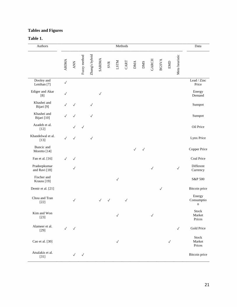
The comparison table of literature review is shown in Table 1. The main objectives of this paper
are as follows:
Checking the cointegration of Bitcoin with three other popular coins, to determining a coin
which has the highest ability to be used as a predictor of Bitcoin price, especially in a
situation that there is little information about Bitcoin;
Forecasting the Bitcoin price based on other coins, using machine learning algorithms such
as Linear Regression (LR), Gradient Boosting Regressor (GBR), Support Vector Regressor
(SVR), Random Forest Regressor (RFR);
Utilizing Time Series Analysis Models to recognize which coin fits the historical data
better than others in the cointegration process.
3. Methodology
This section is divided into several parts that explain the fundamental of the techniques
used in this paper and the description of the data of four well-known cryptocurrencies. Then, we
clarify the new approach that may give us more insight into the price of Bitcoin based on the other
digital currencies, so these parts will be as follows:
3.1. Data Description
For the practical application, four-digital coins were collected from
coinmarketcap.com from 1st April 2018 to 31st March 2019. These are as follows:
7
Bitcoin
Bitcoin (₿ ) is a digital currency, a type of electronic money. It is decentralized advanced
cash without a national bank or single chairman that can be sent from client to client on the shared
Bitcoin arrange without middle people's requirement.
Exchanges are checked by system hubs through cryptography and recorded in an open
disseminated record called a blockchain. Bitcoin was designed by an obscure individual or
gathering of individuals utilizing the name Satoshi Nakamoto and discharged as open-source
programming in 2009. Bitcoins are made as a fee for an operation known as mining. They can be
dealt with for various fiscal structures, things, and organizations. Research delivered by the
University of Cambridge gauges that in 2017, there were 2.9 to 5.8 million remarkable clients
using a digital currency wallet, the vast majority of them utilizing Bitcoin.
Ethereum
Another type of cryptocurrency is Ethereum, which is founded in 2015. It is based on a
modified version of Nakamoto’s theory. Ethereum was suggested in late 2013 by Vitalik Buterin,
a digital cash specialist and programmer. Ethereum is the pioneer for blockchain-based smart
contracts. Smart contracts take into account code to be run precisely as customized with no
plausibility of downtime, control, and deceit or outsider impedance on the blockchain. The worth
of the Ethereum token developed more than 13,000 percent in 2017, to over $1400. By September
2018, it had decreased to $200.
Litecoin
Litecoin (LTC or Ł) is a distributed digital money and open-source programming project
discharged under the MIT/X11 license. The creation and exchange of coins depend on an open-
source cryptographic convention and aren't overseen by any focal expert. Litecoin was an early
Bitcoin spinoff or altcoin, beginning in October 2011. In specialized subtleties, Litecoin is about
indistinguishable to Bitcoin.
Zcash
Zcash is a digital currency gone for utilizing cryptography to improve its clients' security
contrasted with other digital money, such as Bitcoin. Zcash has a total fixed supply of 21 million
units. Exchanges can be "transparent" and like Bitcoin exchanges, in which case a t-addr constrains
them, or can be a kind of zero-learning verification called zk-SNARKs; the exchanges are then
said to be "shielded" and are constrained by a z-addr.
3.2. Statistical Models and Artificial Intelligence Methods
This part explains some conventional statistical models like AR, MA, ARIMA, and ANFIS
as intelligent methods that combine both fuzzy and artificial neural networks.
3.2.1. Autoregressive (AR)
An autoregressive model illustrates a sort of random process; all things considered, it is
used to define time-fluctuating procedures in nature, financial aspects, etc. In machine learning,
an AR model gains from a series of timed steps and accepts estimations from past activities as
inputs for a regression model to foresee the next time step's value. AR models exploit how time-
series information is successive – it's essential to preserve the order or sequence of the data to
8
make exact forecasts. The forecasts for autoregressive models are regressed on previous
observations in the time series. These models use weighted sums of past values to figure future
values. The notation AR(p) shows an autoregressive model of order p. It is characterized as:
1
p
t i t i t
i
X c X
(1)
Where 𝜑𝑖 is the parameter of the model, c is a constant, and 𝜀𝑡 is white noise – A white noise
process is one with a mean zero and no correlation between its values at different times.
Once the above equation's parameters have been estimated, the autoregression can be used
to forecast an arbitrary number of periods into the future.
3.2.2. Moving Average (MA)
In time series analysis, the Moving Average model (MA model), moreover called moving-
average procedure, is a typical methodology for displaying univariate time series. The moving-
average model determines that the upshot variable depends directly on the present and different
past values of a stochastic (imperfectly forecastable) term. A moving average model of order q
(i.e., MA(q)) is characterized as follows:
1 1 ...t t t q t qX (2)
where 𝜇 is the mean of the series, 1,..., q are the parameters of the model and the ,...,t t q
are white noise error terms.
3.2.3. Autoregressive Integrated Moving Average (ARIMA)
ARIMA models are, in principle, the broadest class of models for anticipating a time series
which can be made to be "stationary" by subtracting (if essential), may be related to nonlinear
changes, for example, logging or deflating (if necessary), an ARIMA model is speculation of an
autoregressive and moving average models. Both of these models are fitted to time series
information either to all the more likely comprehend the information or to predict future points in
the series. The AR part of ARIMA specifies that the interest's evolving variable is regressed on its
own lagged values. The MA part denotes that the regression fault is a linear compound of fault
terms whose values coincided at various times in the past. The "I" shows that the data values have
been altered with the diversity between their values and the olden values. Every one of these
attributes aims to fit the model throughout the data beyond what many would consider possible.
ARIMA models are commonly ARIMA(p, d, q) where parameters p, d, and q are positive
integers, p is the order of the autoregressive model, d is the level of subtracting, and q is the order
of the moving average model. This model as follows:
1 1
(1 )(1 ) (1 )d
p qi i
i t i t
i i
L L X L
(3)
3.2.4. Machine Learning (ML)
One of Artificial Intelligence applications is machine learning, which gives systems the
capability to learn and make better from experience without any definitive program spontaneously.
9
Computer programs have developed by accessing data and utilizing it for learning themselves in
machine learning.
The way toward learning starts with perceptions or information to search for patterns in
data and settle on better choices, later on, depending on the precedents. The essential point is to
permit the PCs to adapt naturally without human mediation or help and change activities in like
manner. Machine learning algorithms refer to the type of targets that can divide into regression
models, classification models, clustering models, etc.
3.3. Cointegration
Cointegration is a statistical measurement of a collection (X1, X2, ..., Xk) of time series
variables. If at least two series are exclusively coordinated. In any case, some linear compound has
a lower order of integration; at that point, the series is said to be cointegrated. The three primary
techniques for testing cointegration are:
- Engle-Granger two-step method
- Johansen test
- Phillips–Ouliaris cointegration test
Several types of data are cointegrated; some of them are as follows:
Economic substitutes as heating oil and natural gas, platinum and palladium, corn and
wheat, corn and sugar, etc.
3.4. Our proposal framework
In this part, we provide a brief discussion of the theoretical procedure of the experiment.
Firstly, we analyze the data of the changing price of four different digital currencies to realize the
main trends and figure out if they are stationary or not. As said before, the first purpose of this
paper is to forecast the price of Bitcoin based on the other digital currencies. It is assumed that
price fluctuations in each digital currency follow the random walk process. Therefore, it cannot be
predicted. As it is nonstationary, there are many various ways to make a time series of information
stationery. Several statistical tests determine whether a process is a random walk or not, such as
Dickey-Fuller (DF) test, the Augment Dickey-Fuller (ADF) test, Ng-Perron test, DF-GLS test,
ERS-point optimal test, and Phillips-Perron test. In this paper, we try to make a process (daily
price of Bitcoin) stationary by subtracting the other process. Cointegration was checked to use
different models.
Checking the cointegration of two processes have two steps, we regress the first variable
(Y) on the second variable, so the equation will be Y-bX, and the Augmented Dickey-Fuller test
or any other statistical test should be run on it to check if it is still random walk or not. Estimating
the regression line for checking the cointegration can be executed through the following methods:
1.Ordinary Least Squares (OLS)
2.Fully Modified Ordinary Least Squares (FMOLS)
3.Dynamic Ordinary Least Squares (DOLS)
10
After checking the stationarity condition, statistical time series models as AR, MA,
ARIMA, and neuro-fuzzy model that are categorized as AI models that can be applied on it, also
we try to run a code to tune the parameters based on the performance criteria such as Akaike
Information Criterion (AIC) and Bayesian Information Criterion. Then we try to cover all of the
performance criteria to evaluate each method, such as:
1. Mean Square Error (MSE)
2. Mean Absolute Percentage Error (MAPE)
3. Mean Absolute Error (MAE)
4. Akaike Information Criterion (AIC)
5. Bayesian Information Criterion
4. Data Analysis and Models Deployment
In this section, the behavior of cryptocurrencies’ prices, time series plots, models’
execution, and evaluation criteria are discussed in detail. Then the cointegration between Bitcoin,
as a fixed part, is checked with the other ones.
4.1. Time Series Plots
As mentioned before, cryptocurrencies’ datasets indicated daily price changes throughout
the year. The most crucial application of analyzing time series plot is to determine whether the
process is stationary or not, along with this part. Also, autocorrelation function (ACF) can be a
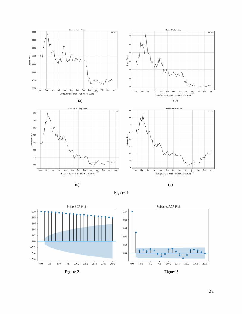
useful method to figure it out. To gain this information, time series are plotted (Figure 1).
As shown in Figure 1, the price fluctuations reach the pick in May and gradually fall until
December. It shows that they are full of changes, making forecasting complex because the price
of cryptocurrencies like stocks is random walks. Hence, they are not predictable, which makes us
use another attribute to forecast them. This attribute is recognized as “return,” which is a
differencing that make the process stationary. In the following figures, firstly, the prices and
returns’ ACF are shown. Secondly, their returns are plotted to make sure differencing works as
what we are expected.
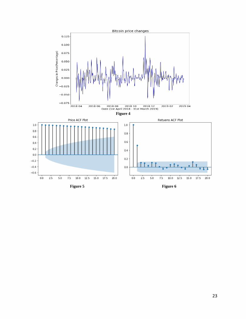
The above figures (Figures 2, 3, and 4) are plotted to show the difference between the
autocorrelation in Bitcoin price and Bitcoin price returns. As shown in Bitcoin prices’ ACF, the
Bitcoin price's ACF plot is not stationary, but we can see that the returns are entirely stationary.
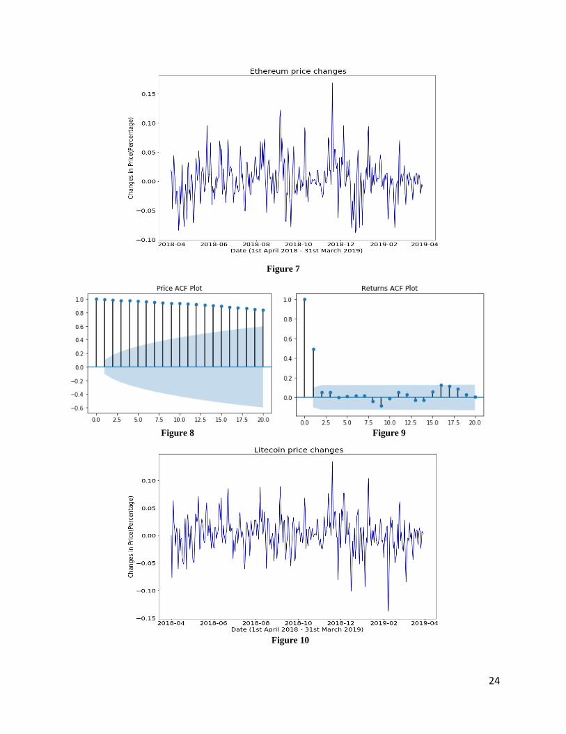
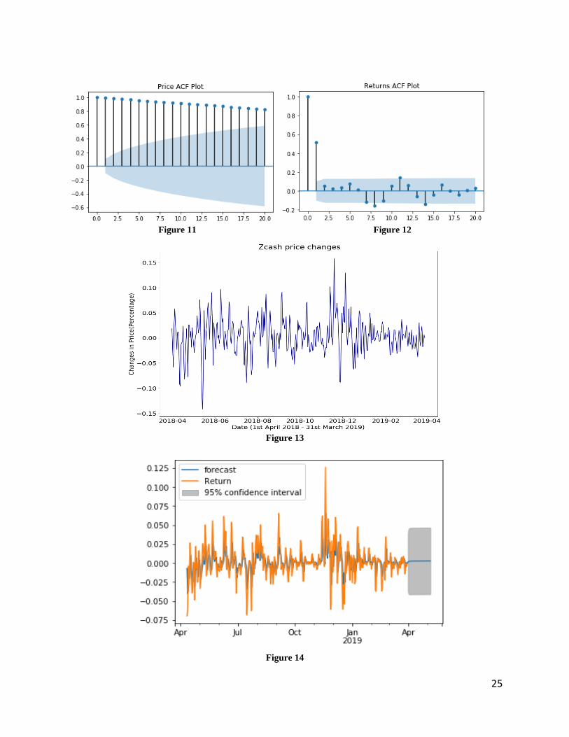
As shown in the following figures (Figures 5, 6, 7, 8, 9, 10, 11, 12, 13), Ethereum,
Litecoin, and Zcash also have the same Bitcoin condition. Their price fluctuations are not
stationary, but we notice that they are stationary if we examine their price returns.
4.2. MA, AR and ARIMA Models for Price Returns
First of all, we apply the ARIMA models to each of the cryptocurrencies’ price returns to
predict a step forecast. We use ARIMA because these models include MA and AR models inside
of it as we apply ARIMA (0, 0, q) and ARIMA (p, 0, 0), respectively. According to the previous
section, all the returns were stationary; thus, they are ready to get models on them to forecast. The
11
ACF plots have shown that returns are not so simple, and we cannot execute a pure AR or MA
model on them. The following graphs contain real values, fitted values, and also the forecasting
part simultaneously. As usual, the confidence interval is about 95% percent. The graphs are as
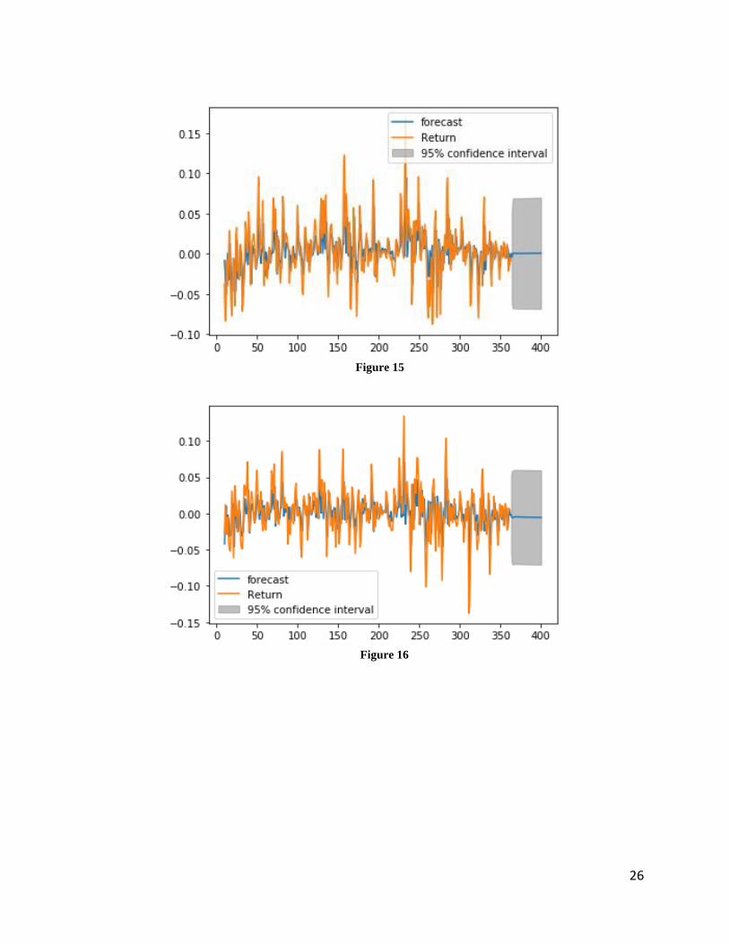
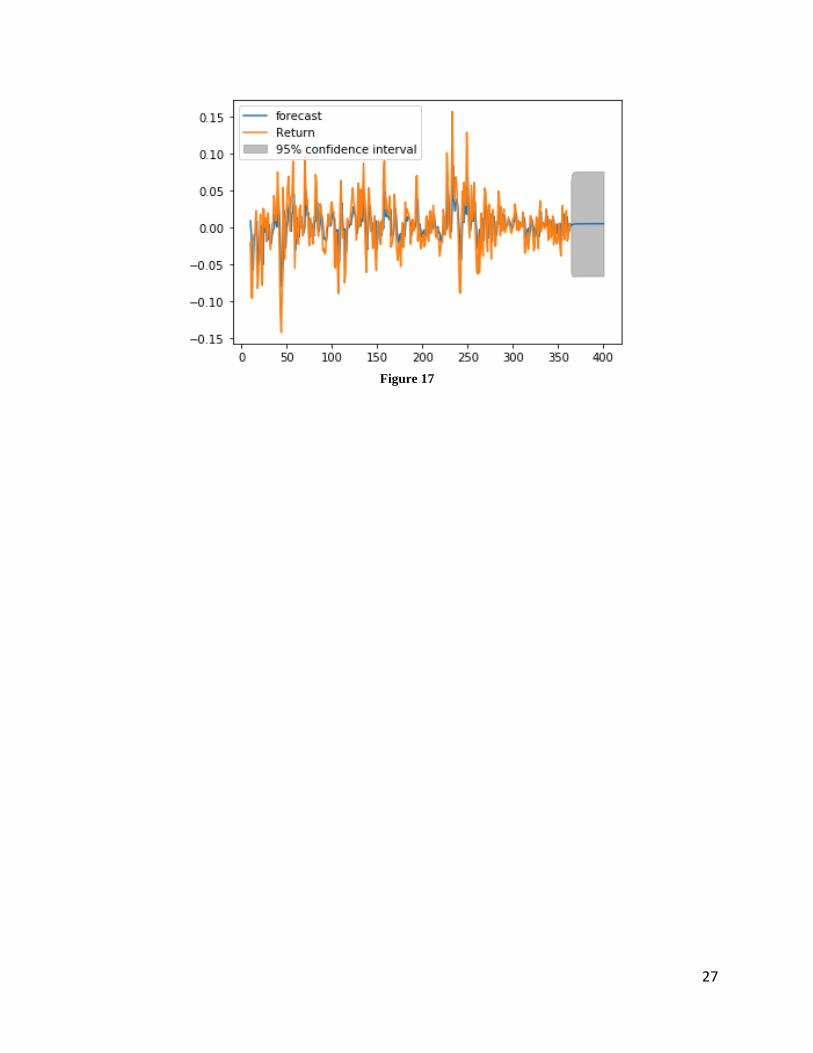
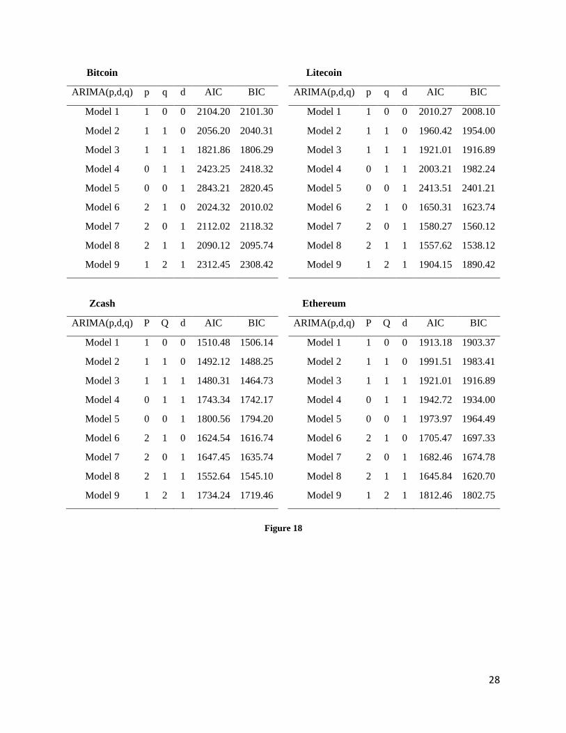
follows (Figures 14, 15, 16, and 17):
Different parameter values have been tested on Bitcoin returns, and the best outcome was
p=1 and q=1 with one difference.
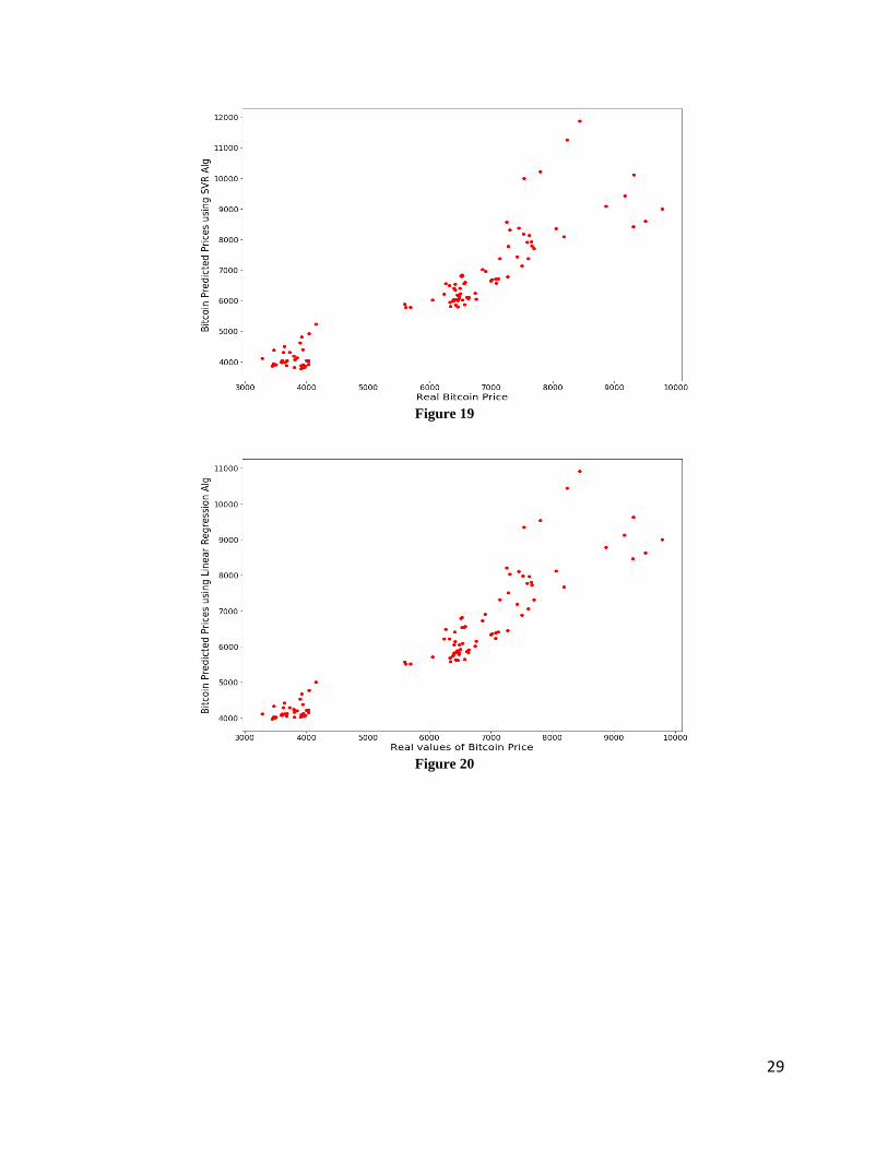
These figures are based on the ARIMA models, and the best values for parameters were
gained using different programs that were coded to achieve the best performance rates. After the
tuning process, we plotted the final results to show the function of the best models. Figure 18
shows the quick results of the programs. The same processes as Bitcoin have been executed for
the rest of them, and the best model for each one is ARIMA(2, 1, 1), ARIMA(2, 1, 1), and
ARIMA(1, 1, 1) for Ethereum, Litecoin, and Zcash, respectively (Figure 18).
4.3. Machine learning prediction
Machine learning algorithms are utilized to predict the Bitcoin price and realize which
cryptocurrencies (Ethereum, Zcash, and Litecoin) impact Bitcoin’s price changes. To use different
ML algorithms, firstly, we need to set a dataset that contains Ethereum’s, Zcash’s, and Litecoin’s
prices as independent variables and Bitcoin’s price as the dependent variable. Then ML algorithms
are applied to find out which cryptocurrencies can forecast the Bitcoin’s price changes without
any data on the trend of the Bitcoin’s price.
Regression methods are one of the forecasting algorithms in machine learning, which
Linear Regression algorithm, Gradient Boosting Regressor algorithm (GBR), Support Vector
Regressor algorithm (SVR), Lasso Regression algorithm, and Random Forest Regressor algorithm
(RFR) are used in this paper to achieve referred goals.
In all of these methods, 80 percent of data assigns to the training part, and the rest of 20 percent
gives it to the testing part. After utilizing methods, MSE is calculated for each of them as an
evaluation criterion. The MSE formula is as follow:
2
1
1ˆ( )
n
i i
i
MSE y yn
(4)
4.3.1. Support Vector Regressor algorithm
Support Vector Machines algorithm (SVM) as an ML method, divided into two parts:
1.Classification and 2.Regression. According to our goal, SVR is utilized with “Linear” kernel,
MSE is calculated, and a comparison figure between real Bitcoin’s price values and predicted ones
by SVR is shown (Figure 19).
MSE = 516804.797833455
4.3.2. Linear Regression algorithm
The linear Regression algorithm is one of the simplest methods among machine learning
algorithms that can produce appropriate answers. The MSE value shows that this method has better
performance in comparison with SVR. The following figure (Figure 20) illustrates the real
Bitcoin’s price values and predicted ones by LR.
12
MSE = 421034.06468415906
4.3.3. Random Forest Regressor algorithm
Another ML algorithm is Random Forest Regression (RFR), an ensemble method formed
by a few Decision Tree methods. RFR can be used in both classifiers and regression forms. This
method's parameter is determined by their users, which the optimal one in this paper achieved
experimentally, 207 trees. According to the MSE value, it shows that this method performs strictly
better than two previous methods (Figure 21).
MSE = 23365.60049452004
4.3.4. Gradient Boosting Regressor algorithm
Another ensemble method as a famous ML algorithm is the Gradient Boosting Regression
(GBR), which contains some parameters. The best state of this method is coming forward when
the number of estimators equal to 100, the learning rate equals 0.12, and the subsample equals 0.6.
By comparing the MSE result of this method with previous methods, GBR is the most appropriate
method to estimate Bitcoin’s price. It is also understandable from the estimated line in the
following figure (Figure 22):
MSE = 18359.190867996942
4.3.5. Lasso Regression algorithm
To gain the second goal, determine the most effective cryptocurrency for predicting
Bitcoin’s price without any information, the Lasso Regression algorithm is applied. The basis of
this method is the data’s variance changing. According to Figure 23, it can be realized that Zcash’s
price trend has the most capability to predict Bitcoin’s price.
As a summary of all applied algorithms, Table 2 gathers the applied method with some
other evaluation criteria. The results shown that the Gradient Boosting Algorithm has the best
accuracy and minimum mean square error.
4.4. Cointegration, our proposal method
In this section, the cointegration between Bitcoin and the other cryptocurrencies check
through two steps. Adding this part can help us predict Bitcoin, as well-known crypto, one step
ahead without any information about its previous trend. We recognize the relation between Bitcoin
and other cryptos to use the best of them for foreseeing Bitcoin price.
As mentioned before, the first step is to regress Bitcoin’s prices on other cryptos. Then we
try to execute the augmented Dickey-Fuller test on them as the second part to figure out whether
they are cointegrated or not. As the residuals are not stationary, first-order differencing is done for
being compatible with ARIMA models. The whole process can be executed via this algorithm in
python environment:
13
Pseudo code:
After applying time series models on residuals, it is necessary to evaluate each model and
decide the appropriate model based on these evaluation criteria. There are different measurements.
Bayesian Information Criterion and Akaike Information Criterion are employed to assess the
models.
2
1 2
T
t
t
ep
AIC LnT T
(5)
2
1 ( )
T
t
t
epLn T
BIC LnT T
(6)
T: number of periods
p: number of estimated parameters
et: residuals
The following graphs (Figure 24) tell about the forms and order of models, the first
condition assigned to cointegration between Bitcoin and Ethereum and ARIMA execution with
the order of p=1, d=1, and q=2:
The regression line is (Equation 7):
_ Pr 3510.527428 7.9343 _ PrBitcoin ice Ethereum ice (7)
P_value of the ADF-test:
3.018049e-05
AIC and BIC of their cointegration:
start
{
Add constant value to a crypto [1];
Result = Ordinary Least Square model (Bitcoin, crypto(x))
Bitcoin = regression_coeff * crypto[1] + residuals
residuals = (Bitcoin - regression_coeff * crypto(x))
Dickey fuller test on residuals
test result
}
end
14
AIC = 4087.4245922612673
BIC = 4192.7285924245916
The second condition assigned to cointegration between Bitcoin and Litecoin and ARIMA
execution with the order of p=0, d=0, and q=2 (it is MA(2)) (Figure 25):
The regression line is (Equation 8):
_ Pr 3120.255075 39.973767 _ PrBitcoin ice Litecoin ice (8)
P_value of the ADF-test:
9.4400204e-05
AIC and BIC of their cointegration:
AIC = 4151.424592183152
BIC = 4166.728592612673
The third condition assigned to cointegration between Bitcoin and Zcash and ARIMA
execution with the order of p=1, d=1, and q=2 (Figure 26):
The regression line is (Equation 9):
_ Pr 3053.563308 20.661674 _ PrBitcoin ice Zcash ice (9)
P_value of the ADF-test:
1.1552e-08
AIC and BIC of their cointegration:
AIC = 3978.591052327704
BIC = 3997.706281805119
The experimental results show that Zcash price can be the best predictor of the Bitcoin
price among two other cryptos as it has the minimum value in AIC and BIC (shown in Table 3).
5. Sensitivity Analysis
There are many different ways to determine the best values of models' parameters.
Sensitivity analysis in time series models refers to changing models' order. For instance, in MA
models, we can change the number of periods that give the trend's smooth shape.
To achieve the best order in these models, we developed an algorithm that iterates different
rankings and results preferred based on the models' evaluation criteria. The following plots (Figure
27) related to some of the time series models which was utilized above:
As shown in regression line estimation by RFR figure, the evaluation criteria, especially BIC,
were calculated using different orders to reach the optimum value (minimum). In the left graph, d
and q were constant (=1), but p iterates and got the optimal order, the same processes have been
15
done for each of the parameters, so as it has done in the right one (p and d are constant). These
procedures have been done for the whole model through the paper.
6. Discussions and Conclusions
Nowadays, many people mine and trade different kinds of cryptocurrencies in a wide range.
As their popularity increased daily, the demands of them enhanced simultaneously. Price
prediction and asset speculation is a high-risk venture. Therefore, the importance of finding an
appropriate way to predict their future values is undeniable. Because of their price volatility, it is
too complicated to apply a stable model for forecasting. Thus, we decided to search for some
features that can help us to predict their price. To find these features and their volatility are mean
reverting, we used to gain the price returns. As an open market determines a cryptocurrency's
value, this presents unique challenges around volatility that most currencies do not face. While
cryptocurrency price prediction is an ever-moving target, market literacy is essential for getting
the most value out of their participation in the crypto economy.
In this paper, Bitcoin's cointegration is checked with three other popular coins to determine
a currency that has the highest ability to be used as a predictor of Bitcoin price, especially when
there is little information about Bitcoin. The Bitcoin price based on other coins is forecasted by
using machine learning algorithms such as Linear Regression (LR), Gradient Boosting Regressor
(GBR), Support Vector Regressor (SVR), and Random Forest Regressor (RFR). Time series
analysis models are applied to recognize which coin fits the historical data better than others in the
cointegration process.
Therefore, at first, the relations among cryptocurrencies have been checked fundamentally
by machine learning algorithms to ensure they have any connections. Then, each cryptocurrency's
price trend had analyzed and plotted daily during a year to realize how they were acting by different
kinds of time series models. After all, a finding of which two cryptocurrencies, Bitcoin as the
stable base, had the most similarity, coming to the main contribution. The importance of finding
the most similarity among three well-known cryptos showed itself when there is no/rare
information on crypto (in this paper, worked on Bitcoin). Using the other crypto can predict what
may happen one step forward. The cointegration between cryptocurrencies is suggested for the
first time in the literature. According to the paper's goal, the cointegration between Bitcoin and
three other cryptocurrencies was studied in four following stages:
1. Bitcoin's price regression on three other cryptos' prices.
2. Execution of ADF-test.
3. ARIMA model implementation on their residuals.
4. Criteria measurement's evaluation.
As a result, among the three cryptocurrencies (Ethereum, Zcash, and Litecoin), Zcash had
the most trend's similarity toward Bitcoin. We also had seen this result by executing the Lasso
Regression algorithm as an ML's method. In other words, as the information on Bitcoin price was
less, the Zcash price information can be used to forecast the Bitcoin price one step forward.
As future work, we intend to work on more cryptocurrencies in a more extended period to
receive more accuracy. Moreover, we plan to apply variate models on the cointegration's estimated
equation. Another common way to predict the price of cryptocurrencies is to utilize deep learning
16
and its algorithms, which, due to their complexity, they are expected to predict prices more
accurately. We plan to implement these algorithms to analyze their performances too.
Nomenclature
𝑋𝑡 model variable in time t
𝑐 constant number of the model
𝜑𝑖 parameter of the model
𝜀𝑡 white noise error
𝜇 mean of the series
𝜃𝑖 parameter of the model
𝑝 the order of the AR model
𝑑 the level of subtracting of ARIMA model
𝑞 the order of the MA model
∅𝑖 parameter of the model
L lag operator for period i
𝑦𝑖 real value of independent variable
𝑦�� estimated value of independent variable
𝑇 number of periods
p number of estimated parameters
𝑒𝑡 residuals error
𝑛 number of observations
Superscript
𝑖 lag index
Subscript
𝑡 time index
17
References
1. Bhattacharya, D., Mukhoti, J., and Konar, A. “Learning regularity in an economic time-
series for structure prediction”, Applied Soft Computing Journal, 76, pp. 31-44 (2019). 2. Corbet, S., Lucey, B., Urquhart, A., and Yarovaya, L. “Cryptocurrencies as a financial asset:
A systematic analysis”, International Review of Financial Analysis, 62, pp. 182-199 (2019). 3. Yang, B., Sun, Y., and Wang, S. “A novel two-stage approach for cryptocurrency analysis”,
International Review of Financial Analysis, 72, (2020). 4. Fryzlewicz, P., Bellegem, S., and Sachs, R. “Forecasting non-stationary time series by
wavelet process modelling”, Annals of the Institute of Statistical Mathematics, 55, pp. 737-764 (2003).
5. Hossain, Z., Rahman, A., Hossain, M., and Karami, J. “Over-Differencing and Forecasting with Non-Stationary Time Series Data”, Dhaka University Journal of Science, 67, pp. 21-26 (2019).
6. Arlinghaus, S.L. “PHB Practical Handbook of Curve Fitting”, In CRC Press, (1994). 7. Dooley, G. and Lenihan, H. “An assessment of time series methods in metal price
forecasting”, Resources Policy, 30(3), pp. 208-217 (2005). 8. Ediger, V., and Akar, S. “ARIMA forecasting of primary energy demand by fuel in Turkey”,
Energy Policy, 35(3), pp. 1701-1708 (2007). 9. Khashei, M. and Bijari, M. “An artificial neural network (p, d, q) model for timeseries
forecasting”, Expert Systems with applications, 37(1), pp. 479-489 (2010). 10. Khashei, M. and Bijari, M. “A novel hybridization of artificial neural networks and ARIMA
models for time series forecasting”, Applied Soft Computing, 11(2), pp. 2664-2675 (2011).
11. Martinez, F., Frias, M., Perez-Godoy, M., and Rivera, A. “Dealing with seasonality by narrowing the training set in time series forecasting with kNN”, Expert Systems With Applications, 103, pp. 38-48 (2018).
12. Azadeh, A. , Moghaddam, M., Khakzad, M., and Ebrahimipour V. “A flexible neural network-fuzzy mathematical programming algorithm for improvement of oil price estimation and forecasting”, Computers & Industrial Engineering, 62(2), pp. 421-430 (2012).
13. Khandelwal, I., Adhikari, R., and Verma, G. “Time Series Forecasting using Hybrid ARIMA and ANN Models based on DWT Decomposition”, Procedia Computer Science, 48(1), pp. 173-179 (2015).
14. Buncic, D. and Moretto, C. “Forecasting copper prices with dynamic averaging and selection models”, North American Journal of Economics and Finance, 33, pp. 1-38 (2015).
15. Laboissiere, L., Fernandes, R., and Lage, G. “Maximum and minimum stock price forecasting of Brazilian power distribution companies based on artificial neural networks”, Applied Soft Computing Journal, 35, pp. 66-74 (2015).
16. Fan, X., Wang, L., and Li, S. “Predicting chaotic coal prices using a multi-layer perceptron network model”, Resources Policy, 50, pp. 86-92 (2016).
18
17. Gangopadhyay, K., Jangir, A., and Sensarma, R. “Forecasting the price of gold: An error correction approach”, IIMB management review, 28(1), pp. 6-12 (2016).
18. Pradeepkumar, D. and Ravi, V. “Forecasting financial time series volatility using particle swarm optimization trained quantile regression neural network”, Applied Soft Computing, 58, pp. 35-52 (2017).
19. Fischer, T. and Krauss, C. “Deep learning with long short-term memory networks for financial market predictions”, European Journal of Operational Research, 270(2), pp. 654-669 (2018).
20. Sezer, O.B. and Ozbayoglu, A.M. “Algorithmic financial trading with deep convolutional neural networks: Time series to image conversion approach”, Applied Soft Computing, 70, pp. 525-538 (2018).
21. Demir, D., Gozgor, G., Lau, C.K.M., and Vigne, S.A. “Does economic policy uncertainty predict the Bitcoin returns? An T empirical investigation”, Finance Research Letters, 26, pp. 145-149 (2018).
22. Chou, JS. and Tran, DS. “Forecasting energy consumption time series using machine learning techniques based on usage patterns of residential householders”, Energy, 165, pp. 709-726 (2018).
23. Kim, H.Y. and Won, C.H. “Forecasting the volatility of stock price index: A hybrid model integrating LSTM with multiple GARCH-type models”, Expert Systems with Applications, 103, pp. 25-37 (2018).
24. Phillips, P., Shi, S., and Yu, J. “Testing for Multiple Bubbles: Historical Episodes of Exuberance and Collapse in the S&P 500”, International economic review, 56(4), pp. 1043-1078 (2013).
25. Bouri, E., Shahzad, J., and Roubaud, D. “Co-Explosivity in the Cryptocurrency Market”, Finance Research Letters, 29, pp. 178-183 (2018).
26. Bouri, E., Gupta, R., and Roubaud, D. “Herding behaviour in cryptocurrencies”, Finance Research Letters, 29, pp. 216-221 (2018).
27. Ji, Q., Bouri, E., Lau, C.K., and Roubaud, D. “Dynamic connectedness and integration in cryptocurrency markets”, International Review of Financial Analysis, 63, pp. 257-272 (2018).
28. Mallqui, D.C. and Fernandes, R.A. “Predicting the direction, maximum, minimum and closing prices of daily Bitcoin exchange rate using machine learning techniques”, Applied Soft Computing, 75, pp. 596-606 (2019).
29. Alameer, Z., Elaziz, M., Ewees, A., Ye, H., and Jianhua, Z. “Forecasting gold price fluctuations using improved multilayer perceptron neural network and whale optimization algorithm”, Resources Policy, 61, pp. 250-260 (2019).
30. Cao, J., Li, Z., and Li, J. “Financial time series forecasting model based on CEEMDAN and LSTM”, Physica A: Statistical Mechanics and its Applications, 519, pp. 127-139 (2019).
31. Atsalakis, G. S., Atsalaki, I. G., Pasiouras, F., Zopounidis, C. “Bitcoin price forecasting with neuro-fuzzy techniques”, European Journal of Operational Research, 276, pp. 770-780 (2019).
32. Bouri, E., Roubaud, D., and Shahzad, J. “Do Bitcoin and other cryptocurrencies jump together?”, The Quarterly Review of Economics and Finance, 76, pp. 396-409 (2019).

19
33. Bouri, E., Lucey, B., and Roubaud, D. “The volatility surprise of leading cryptocurrencies: Transitory and permanent linkages”, Finance Research Letters, 33 (2020).
34. Qureshi, S., Aftab, M., Bouri, E., and Saeed, T. “Dynamic interdependence of cryptocurrency markets: An analysis across time and frequency”, Physica A: Statistical Mechanics and its Applications, 559, (2020).
20
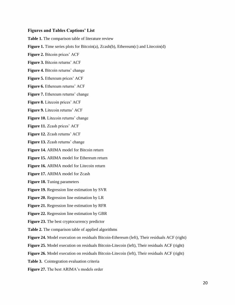
Figures and Tables Captions’ List
Table 1. The comparison table of literature review
Figure 1. Time series plots for Bitcoin(a), Zcash(b), Ethereum(c) and Litecoin(d)
Figure 2. Bitcoin prices’ ACF
Figure 3. Bitcoin returns’ ACF
Figure 4. Bitcoin returns’ change
Figure 5. Ethereum prices’ ACF
Figure 6. Ethereum returns’ ACF
Figure 7. Ethereum returns’ change
Figure 8. Litecoin prices’ ACF
Figure 9. Litecoin returns’ ACF
Figure 10. Litecoin returns’ change
Figure 11. Zcash prices’ ACF
Figure 12. Zcash returns’ ACF
Figure 13. Zcash returns’ change
Figure 14. ARIMA model for Bitcoin return
Figure 15. ARIMA model for Ethereum return
Figure 16. ARIMA model for Litecoin return
Figure 17. ARIMA model for Zcash
Figure 18. Tuning parameters
Figure 19. Regression line estimation by SVR
Figure 20. Regression line estimation by LR
Figure 21. Regression line estimation by RFR
Figure 22. Regression line estimation by GBR
Figure 23. The best cryptocurrency predictor
Table 2. The comparison table of applied algorithms
Figure 24. Model execution on residuals Bitcoin-Ethereum (left), Their residuals ACF (right)
Figure 25. Model execution on residuals Bitcoin-Litecoin (left), Their residuals ACF (right)
Figure 26. Model execution on residuals Bitcoin-Litecoin (left), Their residuals ACF (right)
Table 3. Cointegration evaluation criteria
Figure 27. The best ARIMA’s models order
21
Tables and Figures
Table 1.
Authors Methods Data
A
RIM
A
AN
N
Fu
zzy
met
hod
Zh
ang's
hy
bri
d
SA
RIM
A
SV
R
LS
TM
CA
RT
DM
A
DM
S
GA
RC
H
BG
SV
A
EM
D
Met
a h
euri
stic
Dooley and Lenihan [7]
✓ Lead / Zinc
Price
Ediger and Akar [8]
✓ ✓ Energy
Demand
Khashei and Bijari [9]
✓ ✓ ✓ Sunspot
Khashei and Bijari [10]
✓ ✓ ✓ Sunspot
Azadeh et al. [12]
✓ ✓ Oil Price
Khandelwal et al.
[13] ✓ ✓ ✓ Lynx Price
Buncic and
Moretto [14] ✓ ✓ Copper Price
Fan et al. [16] ✓ ✓ Coal Price
Pradeepkumar and Ravi [18]
✓ ✓ ✓ Different Currency
Fischer and Krauss [19]
✓ S&P 500
Demir et al. [21] ✓ Bitcoin price
Chou and Tran [22]
✓ ✓ ✓ ✓ Energy
Consumption
Kim and Won
[23] ✓ ✓
Stock
Market
Prices
Alameer et al.
[29] ✓ ✓ ✓ Gold Price
Cao et al. [30] ✓ ✓ Stock
Market Prices
Atsalakis et al. [31]
✓ ✓ Bitcoin price
22
(a) (b)
(c) (d)
Figure 1
Figure 2 Figure 3
23
Figure 4
Figure 5 Figure 6
24
Figure 7
Figure 8 Figure 9
Figure 10
25
Figure 11 Figure 12
Figure 13
Figure 14
26
Figure 15
Figure 16
27
Figure 17
28
Bitcoin Litecoin
ARIMA(p,d,q) p q d AIC BIC ARIMA(p,d,q) p q d AIC BIC
Model 1 1 0 0 2104.20 2101.30 Model 1 1 0 0 2010.27 2008.10
Model 2 1 1 0 2056.20 2040.31 Model 2 1 1 0 1960.42 1954.00
Model 3 1 1 1 1821.86 1806.29 Model 3 1 1 1 1921.01 1916.89
Model 4 0 1 1 2423.25 2418.32 Model 4 0 1 1 2003.21 1982.24
Model 5 0 0 1 2843.21 2820.45 Model 5 0 0 1 2413.51 2401.21
Model 6 2 1 0 2024.32 2010.02 Model 6 2 1 0 1650.31 1623.74
Model 7 2 0 1 2112.02 2118.32 Model 7 2 0 1 1580.27 1560.12
Model 8 2 1 1 2090.12 2095.74 Model 8 2 1 1 1557.62 1538.12
Model 9 1 2 1 2312.45 2308.42 Model 9 1 2 1 1904.15 1890.42
Zcash Ethereum
ARIMA(p,d,q) P Q d AIC BIC ARIMA(p,d,q) P Q d AIC BIC
Model 1 1 0 0 1510.48 1506.14 Model 1 1 0 0 1913.18 1903.37
Model 2 1 1 0 1492.12 1488.25 Model 2 1 1 0 1991.51 1983.41
Model 3 1 1 1 1480.31 1464.73 Model 3 1 1 1 1921.01 1916.89
Model 4 0 1 1 1743.34 1742.17 Model 4 0 1 1 1942.72 1934.00
Model 5 0 0 1 1800.56 1794.20 Model 5 0 0 1 1973.97 1964.49
Model 6 2 1 0 1624.54 1616.74 Model 6 2 1 0 1705.47 1697.33
Model 7 2 0 1 1647.45 1635.74 Model 7 2 0 1 1682.46 1674.78
Model 8 2 1 1 1552.64 1545.10 Model 8 2 1 1 1645.84 1620.70
Model 9 1 2 1 1734.24 1719.46 Model 9 1 2 1 1812.46 1802.75
Figure 18
29
Figure 19
Figure 20
30
Figure 21
Figure 22
31
Figure 23
Table 2.
Algorithms Name MSE R2 R2 adjusted
SVR 516804.797833455 0.8345 0.8391
LR 421034.06468415906 0.8652 0.8689
RFR 23365.60049452004 0.9925 0.9927
GBR 18359.190867996942 0.994 0.9942
Figure 24
32
Figure 25
Figure 26
Table 3.
Cryptocurrencies Cointegration AIC BIC
Bitcoin-Ethereum 4087.4245922612673 4192.7285924245916
Bitcoin-Litecoin 4151.424592183152 4166.728592612673
Bitcoin-Zcash 3978.591052327704 3997.706281805119
33
Figure 27
Authors’ Technical Biography:
Negar Maleki: Negar Maleki has a master's degree in Industrial Engineering from the University of Tehran.
Her main research interests are Machine Learning, Data Analysis, Statistical Inferences, Optimization, and
Biomedical Data.
Alireza Nikoubin: Alireza Nikoubin has a master's degree in industrial engineering and is a research
assistant at the University of Tehran. His main research interests are in financial markets and systems
optimization. He is currently working on a method for portfolio optimization using data mining techniques.
Masoud Rabbani: Masoud Rabbani is Professor of Industrial Engineering in the School of Industrial and
Systems Engineering at the University of Tehran. He has published more than 250 papers in international
journals. His research interests include production planning, Maintenance planning, Mixed model assembly
lines planning, inventory management systems, and applied graph theory.
Yasser Zeinali: Yasser Zeinali is a Ph.D. student at University of Alberta school of business. His research
interests are data analytics, machine learning algorithms and its applications in business and healthcare.