Biomolecular Interaction Analysis Using BSA Anti-BSA: Surface Plasmon Resonance Overview: This experiment determines the kinetics and equilibrium constant for a simple bi-molecular protein/protein interaction. Bovine Serum Albumin (BSA), the ligand, is amine coupled to a gold coated surface. The analyte is Anti-BSA Immunoglobulin G (IgG ) which is injected over the surface at a range of concentrations.

Surface Plasmon Resonance Details aside, surface plasmon resonance, SPR, is a very sensitive and convenient method for the determination of the index of refraction of surface bound layers. The index of refraction of a surface bound layer is proportional to the concentration of bound molecules. Any method that gives a signal proportional to concentration can be the basis for thermodynamic or kinetic studies. For example, UV/visible absorption, fluorescence, NMR intensity, NMR chemical shift, reaction enthalpy, radioactivity, and index of refraction can all be used essentially interchangeably. Therefore, SPR is just one of many techniques that can determine the kinetic on and off rates for the interaction of a biomolecule with a ligand. SPR is distinguished by its generality and high sensitivity. The only condition is that one of the binding pair must be attached to a gold-coated surface. Many techniques are available for attaching small molecules, proteins, and oligonucleotides to surfaces, so SPR is an important new technique that is applicable to the study of binding interactions in a wide range of biological systems. SPR is particularly useful in Biological Interaction Analysis, BIA, in immunology. The index of refraction of a substance is given by the ratio of the speed of light in the sample compared to the speed of light in vacuum, n = ν(sample)/ν(vacuum). The index of refraction of a substance is directly related to the molecular polarizability, which in turn depends in large part on molecular size. Therefore, the index of refraction is a completely general property of any molecule. Thus, SPR can be applied to any system. However, the sensitivity increases greatly with molecular size. SPR uses a nice trick to enhance the sensitivity of index of refraction measurements. Under suitable conditions, shining a light beam at a high incidence angle on a thin film of a metal causes the absorption of light and the production of a surface plasmon. The surface plasmon is a collective motion of the electrons near the surface of the metal. The effect is to create electron density waves that propagate along the surface. A useful analogy is to compare the motion of the electrons to the propagation of sound waves. In sound the energy of the wave is propagated in regions of high and low molecule density. Surface plasmons are similar, but with free electrons at the surface. The effect of the plasmon is to create a very strong oscillating electric field near the surface, which is called the evanescent wave. This electric field is greater than would have been produced by the original light beam. This enhanced electric field can interact with any molecules that are adsorbed to the surface, changing the effective propagation speed. A diagram of the geometry for the measurement is given in Figure 1. The heart of the sample cell is a thin, 50-nm, gold film that has been deposited on a glass slide. A prism bends a monochromatic laser beam so that the beam strikes the gold film at a large incidence angle (measured from the normal to the surface). The light is absorbed, propagates along the gold surface as a plasmon, and then is reemitted. The light emerging from the prism has a strong dependence of intensity with angle. Light emitted at the resonance angle undergoes strong

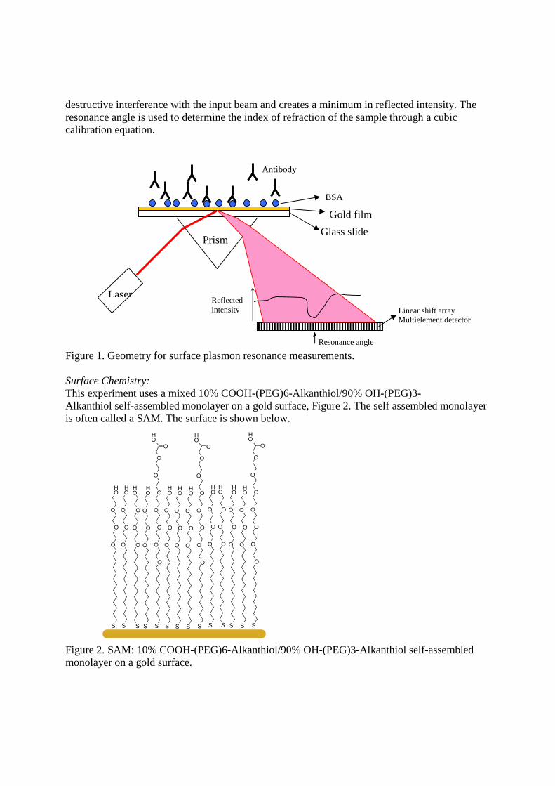
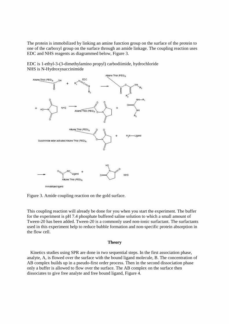
destructive interference with the input beam and creates a minimum in reflected intensity. The resonance angle is used to determine the index of refraction of the sample through a cubic calibration equation. Figure 1. Geometry for surface plasmon resonance measurements. Surface Chemistry: This experiment uses a mixed 10% COOH-(PEG)6-Alkanthiol/90% OH-(PEG)3- Alkanthiol self-assembled monolayer on a gold surface, Figure 2. The self assembled monolayer is often called a SAM. The surface is shown below.

S

O

O

O

OH

S

O

O

O

OH

S

O

O

O

OH

S

O

O

O

OH

S

O

O

O

O

O

O

O

OH

O

S

O

O

O

OH

S

O

O

O

OH

S

O

O

O

OH

S

O

O

O

O

O

O

O

OH

O

S

O

O

O

OH

S

O

O

O

OH

S

O

O

O

OH

S

O

O

O

OH

S

O

O

O

O

O

O

O

OH

O

Figure 2. SAM: 10% COOH-(PEG)6-Alkanthiol/90% OH-(PEG)3-Alkanthiol self-assembled monolayer on a gold surface.

Laser

Prism Glass slide

Gold film

Reflected intensity

BSA

Antibody

Resonance angle

Linear shift array Multielement detector

The protein is immobilized by linking an amine function group on the surface of the protein to one of the carboxyl group on the surface through an amide linkage. The coupling reaction uses EDC and NHS reagents as diagrammed below, Figure 3. EDC is 1-ethyl-3-(3-dimethylamino propyl) carbodiimide, hydrochloride NHS is N-Hydroxysuccinimide

Figure 3. Amide coupling reaction on the gold surface. This coupling reaction will already be done for you when you start the experiment. The buffer for the experiment is pH 7.4 phosphate buffered saline solution to which a small amount of Tween-20 has been added. Tween-20 is a commonly used non-ionic surfactant. The surfactants used in this experiment help to reduce bubble formation and non-specific protein absorption in the flow cell.

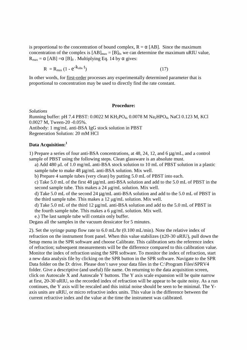
Theory Kinetics studies using SPR are done in two sequential steps. In the first association phase, analyte, A, is flowed over the surface with the bound ligand molecule, B. The concentration of AB complex builds up in a pseudo-first order process. Then in the second dissociation phase only a buffer is allowed to flow over the surface. The AB complex on the surface then dissociates to give free analyte and free bound ligand, Figure 4.

Figure 4. Kinetic time course for one value of the analyte concentration, [A]0. Let [B] be the concentration of the bound molecule and [A] be the solution concentration of the analyte. The surface concentration of bound complex is [AB]. In this experiment, B is bound bovine serum albumin, BSA, and A is the anti-BSA IgG antibody. The association reaction:

A + B

ka

→←

kd

AB (1)

has association rate constant ka and dissociation rate constant kd. The equilibrium constant for the association reaction is KA = ka/kd . Conversely, written as a dissociation the reaction is:

AB

kd

→←

ka

A + B (2)

The equilibrium constant for the dissociation reaction is KD = kd/ka. Assuming the association reaction, Eq. 1, is first order in each reactant and the dissociation reaction is first order in complex gives the overall rate law:

d[AB]

dt = ka [A][B] – k d[AB] (3)

Association Phase: The integrated rate law for the association phase will now be determined. In this experiment during the association phase, the analyte concentration is held constant by flowing the analyte solution over the surface. Therefore, [A] = [A]0, which is the concentration of the antibody sample for each individual run. [A]0 is varied over several separate experiments. Let the total surface concentration of bound protein be [B]0. Then mole balance gives:

[B]0 = [B] + [AB] (4)

where [B] is the concentration of free [B]. Solving for [AB] from Eq. 4 gives the concentration of complex by difference

[AB] = [B] 0 – [B] (5)

Buffer only

Association phase: Analyte, [A]0

Dissociation phase: Buffer only

Inject start Inject end

A + B →← AB AB → A + B

R (uRIU)

Time (sec)

Substitution of Eq. 5 into the rate law gives:

d[AB]

dt = ka [A] 0 [B] – kd([B]0 – [B]) (6)

Collecting terms in [B] gives:

d[AB]

dt = (ka [A] 0 + kd ) [B] – kd[B]0 (7)

Substituting Eq. 5 into the rate derivative gives the rate in terms of the concentration of free B sites:

d[AB]

dt = d([B]0 – [B])

dt = -d[B]dt (8)

which can be substituted into Eq. 7

-d[B]dt = (ka [A] 0 + kd ) [B] – kd[B]0 (9)

At this point several approaches may be taken. For this experiment, kd << ka ; in other words, BSA is a high affinity ligand for the anti-BSA antibody. With this approximation, the second term in Eq. 9 is negligible giving:

-d[B]dt = (ka [A] 0 + kd ) [B] (10)

The constants in Eq. 10 can be grouped to give an effective observed first order rate constant,

kobs = ka [A] 0 + kd. (11)

Then Eq. 10 is seen to be a simple first order rate law:

-d[B]dt = kobs [B] (12)

The integrated rate law gives normal first order decay for the reactant, B:

[B] = [B] 0 e-kobs t (13)

and first order growth for the products:

[AB] = [B] 0 (1 - e-kobs t) (14)

The observed association phase rate constant is determined for a series of analyte concentrations by fitting the kinetic time course for each concentration to Eq. 14. A plot of kobs verses [A]0 then gives a straight line with slope ka and intercept kd, Eq. 11.

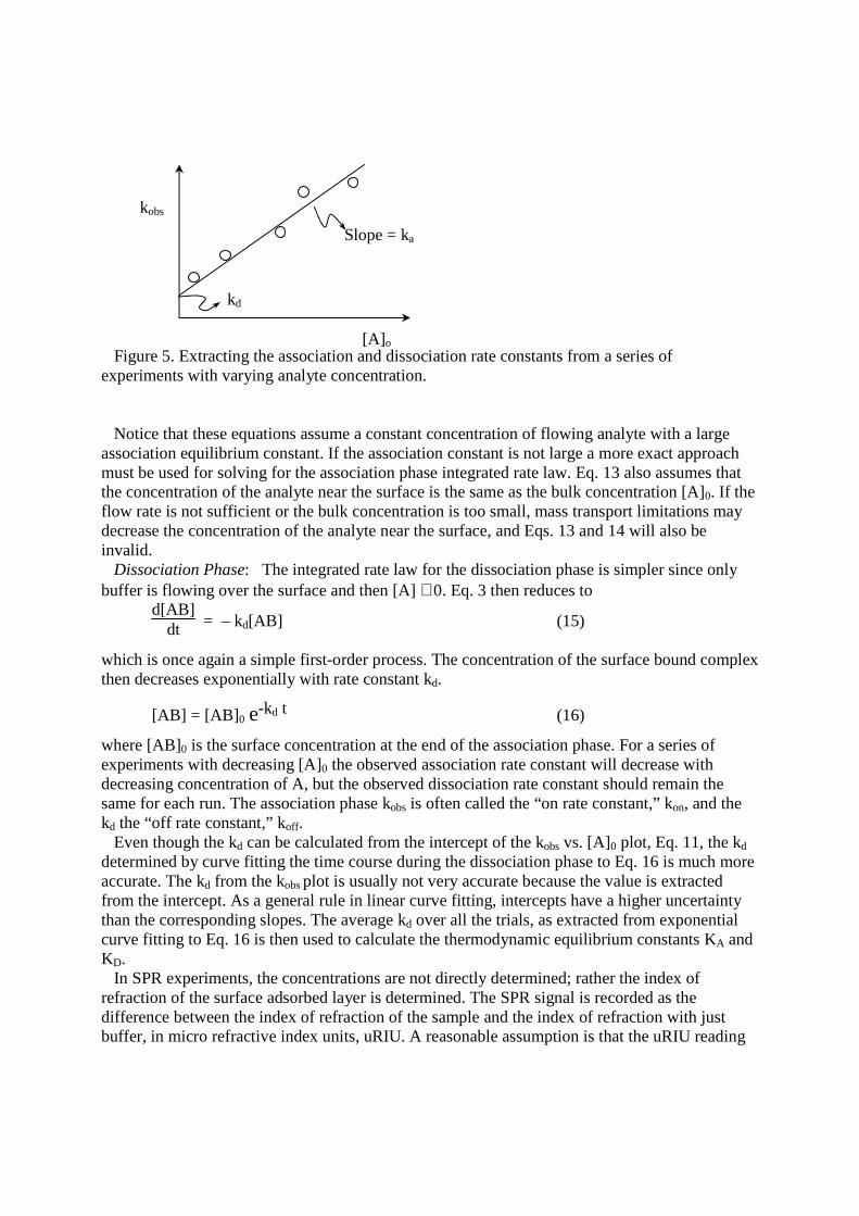
Figure 5. Extracting the association and dissociation rate constants from a series of experiments with varying analyte concentration. Notice that these equations assume a constant concentration of flowing analyte with a large association equilibrium constant. If the association constant is not large a more exact approach must be used for solving for the association phase integrated rate law. Eq. 13 also assumes that the concentration of the analyte near the surface is the same as the bulk concentration [A]0. If the flow rate is not sufficient or the bulk concentration is too small, mass transport limitations may decrease the concentration of the analyte near the surface, and Eqs. 13 and 14 will also be invalid. Dissociation Phase: The integrated rate law for the dissociation phase is simpler since only buffer is flowing over the surface and then [A] ≅ 0. Eq. 3 then reduces to

d[AB]

dt = – kd[AB] (15)

which is once again a simple first-order process. The concentration of the surface bound complex then decreases exponentially with rate constant kd.

[AB] = [AB] 0 e-kd t (16)

where [AB]0 is the surface concentration at the end of the association phase. For a series of experiments with decreasing [A]0 the observed association rate constant will decrease with decreasing concentration of A, but the observed dissociation rate constant should remain the same for each run. The association phase kobs is often called the “on rate constant,” kon, and the kd the “off rate constant,” koff. Even though the kd can be calculated from the intercept of the kobs vs. [A]0 plot, Eq. 11, the kd determined by curve fitting the time course during the dissociation phase to Eq. 16 is much more accurate. The kd from the kobs plot is usually not very accurate because the value is extracted from the intercept. As a general rule in linear curve fitting, intercepts have a higher uncertainty than the corresponding slopes. The average kd over all the trials, as extracted from exponential curve fitting to Eq. 16 is then used to calculate the thermodynamic equilibrium constants KA and KD. In SPR experiments, the concentrations are not directly determined; rather the index of refraction of the surface adsorbed layer is determined. The SPR signal is recorded as the difference between the index of refraction of the sample and the index of refraction with just buffer, in micro refractive index units, uRIU. A reasonable assumption is that the uRIU reading

Slope = ka

kobs

[A] o

kd

is proportional to the concentration of bound complex, R = α [AB]. Since the maximum concentration of the complex is [AB]max = [B]0, we can determine the maximum uRIU value, Rmax = α [AB] =α [B]0 . Multiplying Eq. 14 by α gives:

R = Rmax (1 - e-kobs t) (17)

In other words, for first-order processes any experimentally determined parameter that is proportional to concentration may be used to directly find the rate constant.

Procedure: Solutions Running buffer: pH 7.4 PBST: 0.0022 M KH2PO4, 0.0078 M Na2HPO4, NaCl 0.123 M, KCl 0.0027 M, Tween-20 -0.05%. Antibody: 1 mg/mL anti-BSA IgG stock solution in PBST Regeneration Solution: 20 mM HCl Data Acquisition:1

1) Prepare a series of four anti-BSA concentrations, at 48, 24, 12, and 6 µg/mL, and a control sample of PBST using the following steps. Clean glassware is an absolute must.

a) Add 480 µL of 1.0 mg/mL anti-BSA stock solution to 10 mL of PBST solution in a plastic sample tube to make 48 µg/mL anti-BSA solution. Mix well. b) Prepare 4 sample tubes (very clean) by putting 5.0 mL of PBST into each. c) Take 5.0 mL of the first 48 µg/mL anti-BSA solution and add to the 5.0 mL of PBST in the second sample tube. This makes a 24 µg/mL solution. Mix well. d) Take 5.0 mL of the second 24 µg/mL anti-BSA solution and add to the 5.0 mL of PBST in the third sample tube. This makes a 12 µg/mL solution. Mix well. d) Take 5.0 mL of the third 12 µg/mL anti-BSA solution and add to the 5.0 mL of PBST in the fourth sample tube. This makes a 6 µg/mL solution. Mix well. e.) The last sample tube will contain only buffer.

Degass all the samples in the vacuum dessicator for 5 minutes.

2). Set the syringe pump flow rate to 6.0 mL/hr (0.100 mL/min). Note the relative index of refraction on the instrument front panel. When this value stabilizes (±20-30 uRIU), pull down the Setup menu in the SPR software and choose Calibrate. This calibration sets the reference index of refraction; subsequent measurements will be the difference compared to this calibration value. Monitor the index of refraction using the SPR software. To monitor the index of refraction, start a new data analysis file by clicking on the SPR button in the SPR software. Navigate to the SPR Data folder on the D: drive. Please don’t save your data files in the C:\Program Files\SPRV4 folder. Give a descriptive (and useful) file name. On returning to the data acquisition screen, click on Autoscale X and Autoscale Y buttons. The Y axis scale expansion will be quite narrow at first, 20-30 uRIU, so the recorded index of refraction will be appear to be quite noisy. As a run continues, the Y axis will be rescaled and this initial noise should be seen to be minimal. The Y-axis units are uRIU, or micro refractive index units. This value is the difference between the current refractive index and the value at the time the instrument was calibrated.

3) Each association/dissociation curve represents a different concentration of anti-BSA. Use the same protocol for each concentration injection. A typical series of runs is shown below. Use your buffer blank as your first sample so that you can practice your injection technique.

Figure 6. A typical SPR run. Note all the association/dissociation curves are taken in the same data file. Instead of 20 mM NaOH, this experiment will use 20 mM HCl to regenerate the surface between runs.

a) Turn the Inject valve in load position (counter clockwise). b) Do an air purge, a PBST wash, and an air purge of the sample loop. c) Fill the injection syringe with 2.5 mL of one of the sample solutions. Invert the syringe, pull the barrel down a small amount to empty the needle, tap the syringe to dislodge any bubbles, and carefully expel the bubbles from the syringe needle. Fill the sample loop with the one of the anti-BSA solutions until it comes out of the inject waste port. Don’t’ push the syringe barrel all the way in to avoid injecting bubbles. Leave the syringe in the injection port, to avoid introducing bubbles. d) On the first run, only, start a new data analysis file by clicking on the SPR button in the SPR software. Give a descriptive (and useful) file name. On returning to the data acquisition screen, click on Autoscale X and Autoscale Y buttons. Wait for a minute or two to establish a baseline. e) Turn the inject valve to inject position. Note the time. Mark the Inject time by clicking the Inject button in the SPR software. As the anti-BSA IgG binds to the surface immobilized BSA, the response will increase with time. Let run 7.00 minutes (420 sec). f) Switch the inject valve to load position. Note the time. Mark the dissociation start time by clicking the Buffer button in the SPR software. Anti-BSA IgG will slowly dissociate showing a slow decrease in response. Let run 7 minutes (420 sec). g) Fill the loop with 2 ml of 20 mM HCL. It is not necessary to do an air purge of the loop. h) Turn inject valve to inject and let run at least 4 minutes.

i) Turn the inject valve to load. j) Base line should return to the PBST level as all the anti-BSA IgG is removed. k) Check the amount of PBST buffer in the eluant syringe. Each run requires at least 2 mL of buffer. Do not disconnect the syringe. If necessary, fill the eluant syringe by pulling on the barrel. There are two one-way valves in the eluant lines that allow the syringe to be filled simply by pulling on the syringe barrel. This procedure helps to avoid bubbles. Stop the syringe pump and restart. Note that the arrow on the left-hand side of the pump display screen will be blinking when eluant is flowing. If you refill the syringe, check the cell waste line to ensure that the flow is reestablished. l) Repeat from step (a) above for each concentration of BSA. The plot above shows what you can expect to see as you run the samples.

4). Press the Stop button to finish data acquisition after the last dissociation period. 5). Make sure to do the last HCl regeneration step and then allow PBST to run through the system for about 15 minutes. Replace the PBST eluant reservoir with freshly degassed reagent grade water. Flush the system for about 30 minutes to clean out the cell. Turn off the pump. Ask your instructor to set the prism temperature to 6 °C to preserve the BSA surface for the next laboratory. During these cleaning steps you should continue with the data analysis. Data Analysis:1,2,3

The first step is to align all the data curves for each sample in the SPR data acquisition program. Then the data is fit using least squares analysis to extract the association and dissociation rate constants in the Scrubber program. To verify the Scrubber results and to ensure that you know the details of the data analysis, you will also work up the data in Excel. In Excel the observed rate constants are plotted according to Eq. 11 to determine the forward rate constant. Finally the dissociation and association equilibrium constant are determined. The step by step procedure is as follows. Align and Overlay4

Pull down the Post Process menu and choose "Load File and Align…" TheLoad and Align form will be displayed.

a.) Pull down the File menu and choose Open to load your “.TXT” Stripchart File into the upper fixed plot.

b) Scale the plot by clicking AutoX and AutoY, or by typing in axis limit numbers (and pressing REFRESH) or by left mouse dragging as discussed for the main form.

c.) Select each trace (data segment) to overlay by clicking the right mouse button and dragging to the right. Vertical red bars will appear to define the edges of the grabbed region. Once a sufficient number of points is grabbed, the region between the vertical red bars will be highlighted in yellow. Release the mouse button and the ADD button should become enabled. If the ADD button is not enabled and is grayed out, too few or too many points have been grabbed.

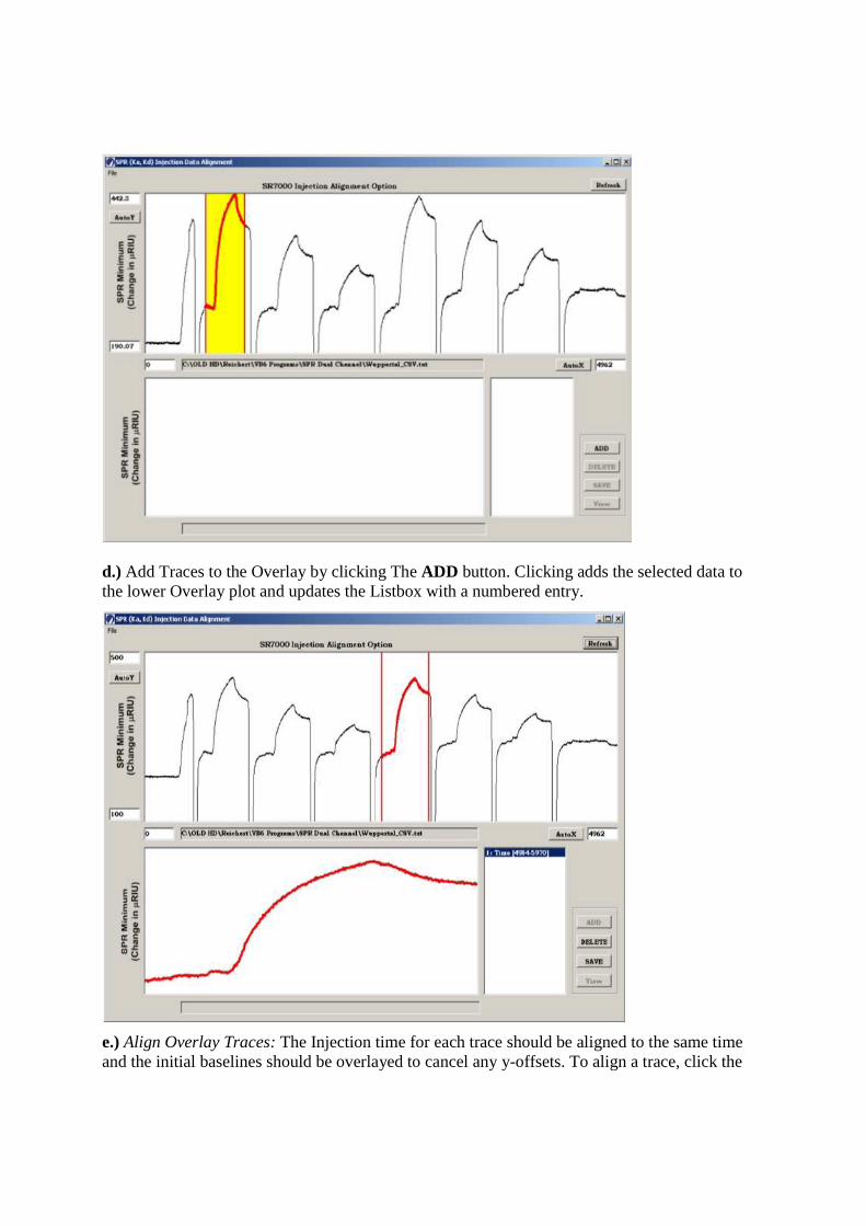
d.) Add Traces to the Overlay by clicking The ADD button. Clicking adds the selected data to the lower Overlay plot and updates the Listbox with a numbered entry.

e.) Align Overlay Traces: The Injection time for each trace should be aligned to the same time and the initial baselines should be overlayed to cancel any y-offsets. To align a trace, click the

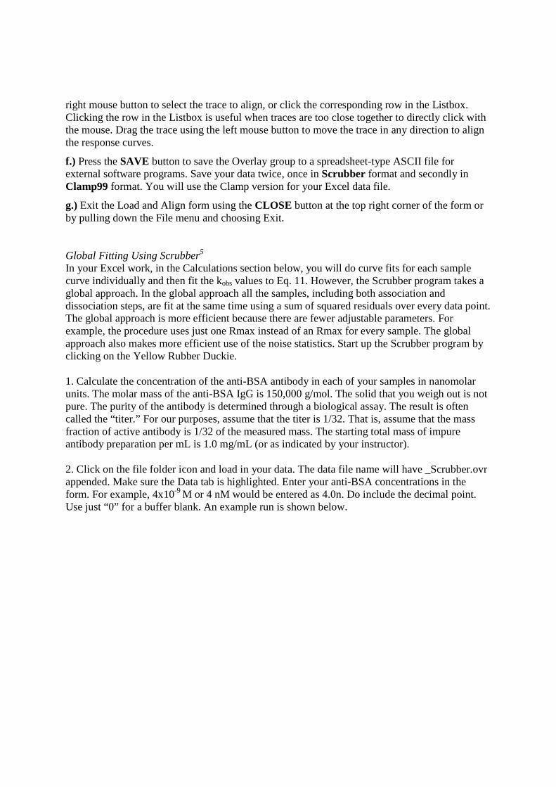
right mouse button to select the trace to align, or click the corresponding row in the Listbox. Clicking the row in the Listbox is useful when traces are too close together to directly click with the mouse. Drag the trace using the left mouse button to move the trace in any direction to align the response curves.

f.) Press the SAVE button to save the Overlay group to a spreadsheet-type ASCII file for external software programs. Save your data twice, once in Scrubber format and secondly in Clamp99 format. You will use the Clamp version for your Excel data file.

g.) Exit the Load and Align form using the CLOSE button at the top right corner of the form or by pulling down the File menu and choosing Exit. Global Fitting Using Scrubber5

In your Excel work, in the Calculations section below, you will do curve fits for each sample curve individually and then fit the kobs values to Eq. 11. However, the Scrubber program takes a global approach. In the global approach all the samples, including both association and dissociation steps, are fit at the same time using a sum of squared residuals over every data point. The global approach is more efficient because there are fewer adjustable parameters. For example, the procedure uses just one Rmax instead of an Rmax for every sample. The global approach also makes more efficient use of the noise statistics. Start up the Scrubber program by clicking on the Yellow Rubber Duckie. 1. Calculate the concentration of the anti-BSA antibody in each of your samples in nanomolar units. The molar mass of the anti-BSA IgG is 150,000 g/mol. The solid that you weigh out is not pure. The purity of the antibody is determined through a biological assay. The result is often called the “titer.” For our purposes, assume that the titer is 1/32. That is, assume that the mass fraction of active antibody is 1/32 of the measured mass. The starting total mass of impure antibody preparation per mL is 1.0 mg/mL (or as indicated by your instructor). 2. Click on the file folder icon and load in your data. The data file name will have _Scrubber.ovr appended. Make sure the Data tab is highlighted. Enter your anti-BSA concentrations in the form. For example, 4x10-9 M or 4 nM would be entered as 4.0n. Do include the decimal point. Use just “0” for a buffer blank. An example run is shown below.

3. Click on the Zero tab. This section adjusts the initial baseline for each of the kinetics runs. Positions the green and red lines to include the flat portion of the baseline before the injection. Drag the lines using the left mouse button. Click on the Zero box. The pre-injection baselines should be set to zero.

You can zoom in on a region of a plot by first drawing a box around an area of interest using the left mouse button (click+drag). You can drag only within the plot axes. Then right click in the plot area and choose Zoom In. To return to the automatic scaling, right click and choose Zoom Out.

4. Click on the Crop tab. This section adjusts the total time interval for each of the kinetics runs. Position the red and blue lines to include the useful portion of the kinetic traces. Do include the pre-injection baselines. Click on the Crop box.

5. Click on the Align tab. This section adjusts the injection times so that they are all equal. Position the red and blue lines to include the inject time for all the traces. Click on the Align box.

Zoom in on the curves around the injection time to verify that the alignment was done correctly. With appropriate time limits, most (if not all) curves should align to zero at the base of their steepest slopes. However, some curves with ambiguous start times may misalign. Choose the data trace to adjust by clicking on the up and down arrow keys in the Set Injection time box. Manually align individual curves by clicking the left and right arrow keys.

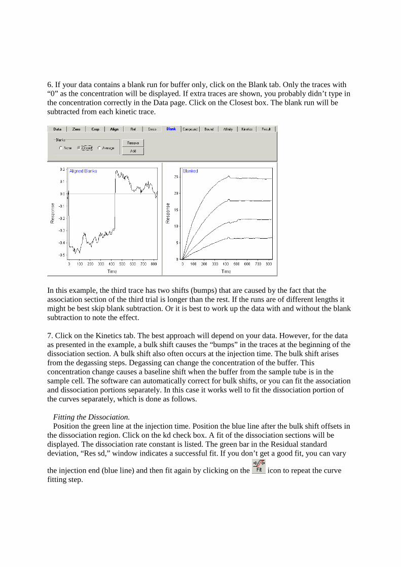
6. If your data contains a blank run for buffer only, click on the Blank tab. Only the traces with “0” as the concentration will be displayed. If extra traces are shown, you probably didn’t type in the concentration correctly in the Data page. Click on the Closest box. The blank run will be subtracted from each kinetic trace.

In this example, the third trace has two shifts (bumps) that are caused by the fact that the association section of the third trial is longer than the rest. If the runs are of different lengths it might be best skip blank subtraction. Or it is best to work up the data with and without the blank subtraction to note the effect. 7. Click on the Kinetics tab. The best approach will depend on your data. However, for the data as presented in the example, a bulk shift causes the “bumps” in the traces at the beginning of the dissociation section. A bulk shift also often occurs at the injection time. The bulk shift arises from the degassing steps. Degassing can change the concentration of the buffer. This concentration change causes a baseline shift when the buffer from the sample tube is in the sample cell. The software can automatically correct for bulk shifts, or you can fit the association and dissociation portions separately. In this case it works well to fit the dissociation portion of the curves separately, which is done as follows. Fitting the Dissociation. Position the green line at the injection time. Position the blue line after the bulk shift offsets in the dissociation region. Click on the kd check box. A fit of the dissociation sections will be displayed. The dissociation rate constant is listed. The green bar in the Residual standard deviation, “Res sd,” window indicates a successful fit. If you don’t get a good fit, you can vary

the injection end (blue line) and then fit again by clicking on the icon to repeat the curve fitting step.

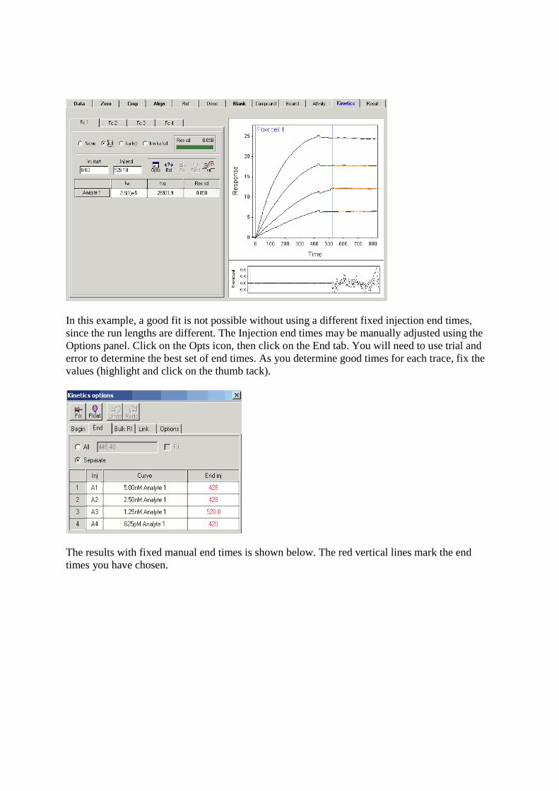
In this example, a good fit is not possible without using a different fixed injection end times, since the run lengths are different. The Injection end times may be manually adjusted using the Options panel. Click on the Opts icon, then click on the End tab. You will need to use trial and error to determine the best set of end times. As you determine good times for each trace, fix the values (highlight and click on the thumb tack).

The results with fixed manual end times is shown below. The red vertical lines mark the end times you have chosen.

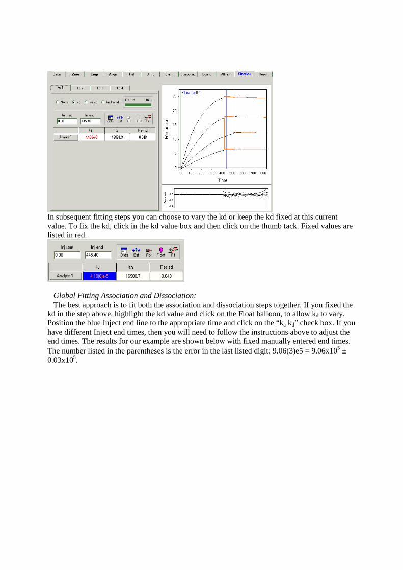
In subsequent fitting steps you can choose to vary the kd or keep the kd fixed at this current value. To fix the kd, click in the kd value box and then click on the thumb tack. Fixed values are listed in red.

Global Fitting Association and Dissociation: The best approach is to fit both the association and dissociation steps together. If you fixed the kd in the step above, highlight the kd value and click on the Float balloon, to allow kd to vary. Position the blue Inject end line to the appropriate time and click on the “ka kd” check box. If you have different Inject end times, then you will need to follow the instructions above to adjust the end times. The results for our example are shown below with fixed manually entered end times. The number listed in the parentheses is the error in the last listed digit: 9.06(3)e5 = 9.06x105 ± 0.03x105.

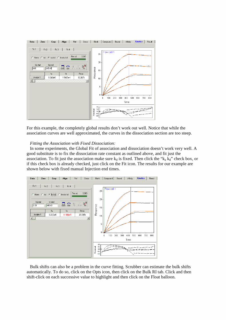
For this example, the completely global results don’t work out well. Notice that while the association curves are well approximated, the curves in the dissociation section are too steep. Fitting the Association with Fixed Dissociation: In some experiments, the Global Fit of association and dissociation doesn’t work very well. A good substitute is to fix the dissociation rate constant as outlined above, and fit just the association. To fit just the association make sure kd is fixed. Then click the “ka kd” check box, or if this check box is already checked, just click on the Fit icon. The results for our example are shown below with fixed manual Injection end times.

Bulk shifts can also be a problem in the curve fitting. Scrubber can estimate the bulk shifts automatically. To do so, click on the Opts icon, then click on the Bulk RI tab. Click and then shift-click on each successive value to highlight and then click on the Float balloon.

In this specific example, the automatic Bulk RI corrections don’t work out well at all. If the automatic fitting doesn’t determine appropriate bulk shifts, you can manually enter values and fix them (highlight each and click on the thumb tack). By trial and error a reasonable bulk shift was manually set for this example.

The resulting fit with fixed kd, Injection end times, and bulk shifts is given below. The results are still not great, but the fits do have an overall smallish residual standard deviation.

Notice that the inclusion of bulk shifts hasn’t helped the final fit residual standard deviation. The value of 0.502 is greater than the 0.369 value obtained above. For our specific example, it might

be better to take the fit values without the bulk shift correction. However, doing the fitting in different ways helps to get realistic estimates of the fit uncertainties. Certainly, the ka value in this example is not known to better than 5% or worse, even though the value, without bulk shift corrections is listed as 9.23(3)e5, indicating 0.1% precision (0.001/9.233x100).

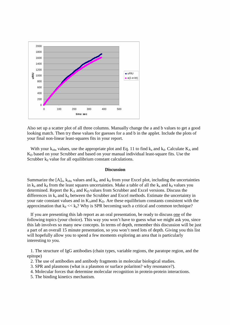
Calculations Having Scrubber do all the calculations is statistically efficient, however, the true uncertainty of the results are not easily revealed. Using the Clamp version of your data file, import the data into Excel. Find the association portion of each run in the data file. Cut and paste the time and uRIU data for each run into a separate area of your spreadsheet. Make sure to set the injection time as time 0. Then use the nonlinear Web applet from the PChem home page: http://www.colby.edu/chemistry/PChem/scripts/lsfitpl.html to find the kobs values for each run. Non-linear curve fitting is not an automatic procedure; guesses must be input for the fit parameters. If the guesses are close enough, the procedure will converge to the best fit results. If the guesses aren’t close enough, the procedure may not converge. Use the Rmax from Scrubber to make a good guess for the “a” parameter. Reasonable guesses for kobs are in the 0.0005 to 0.005 s-1 range. If your curve fit does not converge, try the following two tricks: Trick 1: Scroll down in the text box in the applet to find the final fit parameters. Even though the curve fit didn’t converge, these results are probably better guesses for the a and b parameters than you started with. Try using these final, unconverged values for the initial guesses and try fitting again. Trick 2: For noisy data, trick 1 may not help. In that case a little graphing in Excel will help to narrow in on a better guess. In your Excel spreadsheet, make a column alongside your refractive index column for trial values of a*(1-exp(-b*t)). Here are the first few rows of such a spreadsheet:

vary these

a= 2564 b= 0.002914 t uRIU a(1-e-bt)

0 0 0 2 25.5 14.89953 4 33.5 29.71248 6 45.1 44.43936 8 60.4 59.08065

10 75.4 73.63686 12 93.3 88.10849 14 107.5 102.496 16 122 116.7999 18 135.5 131.0207 20 148.5 145.1589 22 161.4 159.2149 24 174.8 173.1892

0

200

400

600

800

1000

1200

1400

1600

1800

2000

0 100 200 300 400 500

time sec

uR

IU uRIU

a(1-e-bt)

Also set up a scatter plot of all three columns. Manually change the a and b values to get a good looking match. Then try these values for guesses for a and b in the applet. Include the plots of your final non-linear least-squares fits in your report. With your kobs values, use the appropriate plot and Eq. 11 to find ka and kd. Calculate KA and KD based on your Scrubber and based on your manual individual least-square fits. Use the Scrubber kd value for all equilibrium constant calculations.

Discussion Summarize the [A]o, kobs values and ka, and kd from your Excel plot, including the uncertainties in ka and kd from the least squares uncertainties. Make a table of all the ka and kd values you determined. Report the KA and KD values from Scrubber and Excel versions. Discuss the differences in ka and kd between the Scrubber and Excel methods. Estimate the uncertainty in your rate constant values and in KAand KD. Are these equilibrium constants consistent with the approximation that kd << ka? Why is SPR becoming such a critical and common technique?

If you are presenting this lab report as an oral presentation, be ready to discuss one of the following topics (your choice). This way you won’t have to guess what we might ask you, since this lab involves so many new concepts. In terms of depth, remember this discussion will be just a part of an overall 15 minute presentation, so you won’t need lots of depth. Giving you this list will hopefully allow you to spend a few moments exploring an area that is particularly interesting to you. 1. The structure of IgG antibodies (chain types, variable regions, the paratope region, and the epitope) 2. The use of antibodies and antibody fragments in molecular biological studies. 3. SPR and plasmons (what is a plasmon or surface polariton? why resonance?). 4. Molecular forces that determine molecular recognition in protein-protein interactions. 5. The binding kinetics mechanism.

6. The relationships among index of refraction, relative permittivity, polarizability, and molecular size. 7. Other typical SPR based biological interaction analysis studies and why specifically SPR was used. 8. Typical uses of SPR in studies of thin films, especially in non-biological studies. 9. The potential for the use of SPR as a portable chemical sensor in the detection of weapons of mass destruction or environmental areas. Literature Cited: 1. P. Schuck, “Reliable determination of binding affinity and kinetics using plasmon surface resonance biosensors,” Curr. Opin. Biotechnol, 1997, 8(4), 498. 2. D. G. Myszka, “Kinetic, equilibrium, and thermodynamic analysis of macromolecular interactions with BIACORE,” Methods in enzymology, 2000, 323, 325-40. 3. Myszka, D. G.; Rich, R. L., “Implementing surface plasmon resonance biosensors in drug discovery,” Pharmaceutical Science & Technology Today, 2000, 3(9), 310-317. 4. SPR Data Acquistion Software Manual, Reichert, Inc., Buffalo, N. Y. 2006. 5. D. G. Myszka, “Scrubber-2 Manual,” Center for Biomolecular Interaction Analysis, University of Utah, Salt Lake City, Utah, 2005.