biomolecular applications of poisson-boltzmann...

CHAPTER 5

Biomolecular Applications ofPoisson–Boltzmann Methods

Nathan A. Baker

Department of Biochemistry and Molecular Biophysics, Centerfor Computational Biology, Washington University in St. Louis,School of Medicine, 700 S. Euclid Ave., Campus Box 8036,St. Louis, MO, 63110

INTRODUCTION TO BIOMOLECULARELECTROSTATICS

Throughout the 1990s, biomolecular simulation has become increasinglycommonplace in biology and has gained acceptance as an important biophy-sical method for understanding molecular structure, dynamics, and function.The energetic properties of a biomolecule are determined by a combination ofboth short- and long-range forces. Short-range forces include several compo-nents, such as van der Waals, bonding forces, angular forces, and torsionalinteractions. Long-range forces, on the other hand, are typically dominatedby electrostatic interactions. Because of their slow decay over distance, electro-statics cannot be neglected or truncated in biomolecular modeling; these forcescontribute significantly to molecular interactions at all length scales. As such,methods that enable the accurate and efficient modeling of these interactionsare of central importance in molecular simulation.

The exact behavior of electrostatic interactions in a simulation is gener-ally determined by four factors: molecular charge distributions, solute atomicradii, mobile ionic species, and solvent. Molecular charge distributions are

Reviews in Computational Chemistry, Volume 21edited by Kenny B. Lipkowitz, Raima Larter, and Thomas R. Cundari

Copyright � 2005 John Wiley & Sons, Inc., ISBN: 047168239X

349

often determined by fitting electronic distributions (as obtained from quantummechanical calculations) to static point charges located at the atom centers.1,2

However, several groups have demonstrated that static point charge distribu-tions are not sufficient for the accurate modeling of electrostatics—polarizablemodels with higher order charge distribution moments are often necessaryto reproduce molecular energetics.3,4 Regardless of the charge model details,the molecular charge distribution is intimately connected with the steric para-meters chosen for the solute atoms. Together, charges and radii determinemany of the solvation properties of the molecule. Several good references dis-cuss the various issues associated with charge and radius parameterization of asolute.5–7

This chapter focuses on the various ways the aqueous environment sur-rounding a molecule can be treated during a simulation. Specifically, we willexamine a popular class of models for ions and solvent around a molecule andthe description of electrostatic interactions in the context of these models.Treatments of the ions and solvent around a biomolecule are typically dividedinto two classes: explicit and implicit. As their names imply, these models dif-fer by their treatment of solvent and mobile ions as either explicit particles orimplicitly through some type of continuum model. In general, explicit modelsoffer the greatest detail and potential for accuracy in molecular simulation.However, explicit solvent and ions often account for 90–95% of the atomsin a simulation and can, therefore, severely increase the computational timerequired for determining kinetic and thermodynamic properties with any pre-cision. Implicit solvent methods sacrifice the molecular details of the solvent inreturn for far fewer degrees of freedom to be sampled in the simulation. Theresult is a substantial decrease in the computational resources required toobtain converged simulation observables. Because of this decrease in compu-tational requirements, implicit solvent methods often enable much better sam-pling of larger systems than do traditional explicit solvent approaches.However, this increase in length and size of molecular simulations comes atthe cost of a simplistic treatment of water and ions that does not performwell under all circumstances.

This chapter will focus on the applications of implicit solvent methodsand the tools available for employing these techniques in computational chem-istry and biology. Additionally, some potential pitfalls associated with thesemethods will be described in an effort to help users avoid problems causedby overzealous application. Given its place as a benchmark for many implicitsolvent methods, particular emphasis will be placed on the Poisson–Boltzmann(PB) equation. This chapter is designed to supplement the excellent review ofPB theory by Gene Lamm, which recently appeared in this series.8 Readersare strongly encouraged to read Lamm’s chapter as preparation for thepresent discussion of the algorithms and applications associated with the PBequation.

350 Biomolecular Applications of Poisson–Boltzmann Methods

SIMPLIFYING THE SYSTEM: IMPLICIT SOLVENTMETHODS

As mentioned, implicit solvent methods are approximations designed tosimplify the description of the aqueous environment around molecules andthereby reduce the degrees of freedom in a simulation. This section outlinesthe various methods by which solvent-mediated polar and apolar interactionsare described in an implicit solvent setting.

Before discussing the various implicit solvent methods, it is useful tobriefly mention the circumstances in which an explicit description of solventstructure is desirable. In general, explicit solvent methods should be used bychemists where the detailed interactions between solvent and solute are impor-tant. Some example of such situations include solvent finite size effects in ionchannels,9 strong solvent-solute interactions,10 strong solvent coordination ofionic species,11 and saturation of solvent polarization near membranes.12 Like-wise, implicit descriptions of mobile ions are also inappropriate under somecircumstances (cf. See Holm et al.13 for an excellent review), including highion valency or strong solvent coordination, specific ion-solute interactions,and high local ion densities. Potential users of implicit solvent methods areadvised to keep in mind the underlying physics when employing these meth-ods. Although implicit solvent techniques can substantially accelerate biomo-lecular modeling, the ability to quickly compute the wrong answer does littleto help the simulator.

Polar Interactions

Although numerous methods exist for computing polar interactions in animplicit solvent setting, this section gives only a brief overview of some of themost popular methods available. Interested readers should refer to the reviewsby Simonson14 and Roux15 for a more comprehensive overview of availableimplicit solvent methods.

The Debye–Huckel Law:16

f xð Þ ¼ qe�kkx�x0k

e k x � x0 k

provides the simplest description of the electrostatic potential fðxÞ because ofa point charge of magnitude q located at position x0 in a homogeneous polar-izable medium of dielectric constant e. The ionic strength of the solution(determined by the concentration of mobile ion species) is represented bythe screening parameter

k2 ¼ 8pI

1000eRT

Simplifying the System: Implicit Solvent Methods 351

where I is the ionic strength (in molarity, M), R is the gas constant, and T isthe temperature (in Kelvin). The Debye–Huckel law reduces to Coulomb’s lawat zero ionic strength ðk ! 0Þ, providing a description of charges at infinitedilution in a polarizable continuum. Debye–Huckel or Coulombic potentialsobey superposition principles, i.e., the potential caused by a sum of chargesis equivalent to the sum of the potentials because of the isolated charges.

Unfortunately, most biological systems of interest cannot be described asa homogeneous dielectric medium—biomolecular interiors often have signifi-cantly lower polarizabilities than their aqueous surroundings. Therefore, bio-molecular electrostatics typically cannot be modeled by Debye–Huckel orCoulomb equations. However, because of their simplicity and relative easeof evaluation, such equations are attractive bases for the modeling of biomo-lecular electrostatics. Therefore, it is not surprising that these equations werethe starting points for early algorithms that described the inhomogeneous nat-ure of biomolecular systems.

These simpler early models include distance-dependent dielectric func-tions,6,17 reaction field treatments,18–21 and generalized Born (GB) mod-els.22–27 Of these, GB models are arguably the most popular. GB methodswere introduced by Still et al. in 199023 and have been progressively refinedby several other researchers.24–27 GB methods are based on the Born ion, acanonical electrostatics model describing the electrostatic potential and solva-tion energy of a spherical ion28 (see also the later section on solvation-freeenergies). With the GB method, we use an analytical expression based onthe Born ion model to approximate the electrostatic potential and solvationenergy of small molecules. Although it fails to capture all of the details ofmolecular structure and ion distributions provided by more rigorous mod-els,27,29–31 such as the Poisson–Boltzmann equation, it has gained popularityand continues to be vigorously developed, as it is a very rapid method for eval-uating approximate forces and energies for solvated molecules. Recently, anexcellent critical comparison of GB and PB methods was presented by Feiget al.;32 interested readers should refer to this review for relative speeds andaccuracies of GB and PB techniques.

Poisson–Boltzmann methods offer a compromise between faster, butmore approximate models such as GB, and more detailed explicit solventand integral equation techniques.33 The remainder of this chapter is devotedto discussion of the implementation and application of PB and relatedmethods.

Nonpolar Interactions

An important aspect of implicit solvent models is their ability to treatapolar energetics originating from solvent-mediated interactions. In general,apolar methods have been developed separately from their polar counterparts;none of the methods described in the previous section requires a specific apolar


treatment. The apolar term plays an important role in electrostatic force cal-culations; solvation energies/forces obtained from more detailed implicit sol-vent methods (PB and GB) calculations work to maximize the solvent–soluteboundary surface area, thereby providing the maximum solvation for the bio-molecule. Apolar interactions, on the other hand, tend to bias the systemtoward conformations with minimum surface area. The net effect of the polarand apolar solvation terms is a balance of opposing forces determined by thedetails of the molecular structure.

Apolar interactions are generally modeled by either scaled-particle theo-ry methods34,35 or solvent-accessible surface area techniques,36–40 althoughmore rigorous methods have been suggested.41–43 Scaled-particle theories(SPTs) provide apolar interactions in terms of the work required to insert aspherical cavity into a liquid; the resulting energies are usually given as a func-tion of the solute radius and surface area. Solvent-accessible surface area-based models (see Figure 1) are, in essence, a simpler version of scaled-particletheories. Solvent-accessible surface area (SASA) methods relate apolar energiesand forces by one or more ‘‘surface tension’’ constants of proportionality thatare either chosen globally36–38 or for specific atom types.39,40 However,because of the delicate balance between polar and apolar interactions and theirimpact on the results of the simulation, the choice of surface tension constants

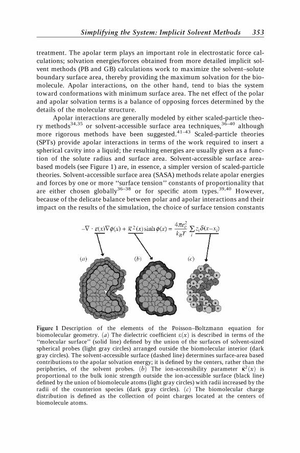
Figure 1 Description of the elements of the Poisson–Boltzmann equation forbiomolecular geometry. ðaÞ The dielectric coefficient eðxÞ is described in terms of the‘‘molecular surface’’ (solid line) defined by the union of the surfaces of solvent-sizedspherical probes (light gray circles) arranged outside the biomolecular interior (darkgray circles). The solvent-accessible surface (dashed line) determines surface-area basedcontributions to the apolar solvation energy; it is defined by the centers, rather than theperipheries, of the solvent probes. ðbÞ The ion-accessibility parameter �kk2ðxÞ isproportional to the bulk ionic strength outside the ion-accessible surface (black line)defined by the union of biomolecule atoms (light gray circles) with radii increased by theradii of the counterion species (dark gray circles). ðcÞ The biomolecular chargedistribution is defined as the collection of point charges located at the centers ofbiomolecule atoms.

Simplifying the System: Implicit Solvent Methods 353

for SASA methods is still more art than science and often depends on the par-ticular system under consideration.

POISSON–BOLTZMANN THEORY: A BRIEFOVERVIEW

This section provides a brief overview of PB theory; however, the inter-ested reader is urged to read the much more comprehensive treatmentprovided by Gene Lamm in vol. 19 of this series.8 As mentioned, thePoisson–Boltzmann equation is obtained from a continuum description ofthe solvent and counterions surrounding a biomolecule.13,44-46 Althoughnumerous derivations of the PB equation are based on statistical mechanics,13,33

the simplest begins with Poisson’s equation:47

�r � eðxÞrjðxÞ ¼ rðxÞ ½1

for x 2 �, the basic equation for describing the electrostatic potential jðxÞgenerated by a charge distribution rðxÞ in a continuum model of a polarizablesolvent with dielectric constant eðxÞ. This equation is generally solved in afinite domain � with the potential specified as gðxÞ on the domain boundaryq�:

jðxÞ ¼ gðxÞ ½1b

for x 2 q�. This Dirichlet boundary condition usually employs an analytic,asymptotically correct form of the potential (Coulomb’s law or Debye–Huckel) for gðxÞ. Therefore, to ensure the applicability of the boundarycondition, the domain must be sufficiently large and the boundaries reasonablydistant (usually a few Debye or Bjerrum lengths) from the biomolecule.

To obtain the PB equation from the Poisson equation, we need to con-sider the two types of charge distributions present in biomolecular systems.First, the partial atomic charges are usually modeled as a ‘‘fixed’’ charge dis-tribution:

rf ðxÞ ¼4pe2

c

kT

XM

i¼1

Qidðx � xiÞ ½2

which describes the M atomic partial charges of the biomolecule as delta func-tions dðx � xiÞ located at the atom centers fxig with magnitudes fQig. Thescaling coefficients ensure the dimensionless form of the potential and includeec, the charge of an electron, and kT, the thermal energy of the system. Addi-tionally, the contributions of counterions are modeled as a continuous ‘‘charge


cloud’’ described by a Boltzmann distribution, giving rise to the ‘‘mobile’’charge distribution

rmðxÞ ¼4pe2

c

kT

Xm

j¼1

cjqj exp �qjjðxÞ � VjðxÞ� �

½3

for m counterion species with charges fqjg, bulk concentrations fcjg, andsteric potentials fVjg (i.e., potentials that prevent biomolecule-counterionoverlap). In the case of a monovalent electrolyte such as NaCl, Eq. [3] reduces to

rmðxÞ ¼ ��kk2ðxÞ sinhjðxÞ ½4

where the coefficient �kk2ðxÞ describes both ion accessibility (via exp½�VðxÞ)and bulk ionic strength. Combining the expressions for the charge distribu-tions (Eqs. [2] and [4]) with Poisson’s equation (Eq. [1]) gives the Poisson–Boltzmann equation for a 1-to-1 electrolyte:

�r � eðxÞrjðxÞ þ �kk2ðxÞ sinhjðxÞ ¼ 4pe2c

kT

XM

i¼1

Qidðx � xiÞ ½5

for x 2 �, where jðxÞ ¼ gðxÞ for x 2 q�. As described, details of the biomo-lecular structure enter into the coefficients of the PB equation (see Figure 1).The dielectric function eðxÞ has been represented by a variety of models,48–52

which typically involve a relatively abrupt change in the dielectric coefficientnear the molecular surface.

The ‘‘full’’ or nonlinear form of the problem given in Eq. [5] is often sim-plified to the linearized PB equation by replacing the sinhjðxÞ term with itsfirst-order approximation, sinhjðxÞ � jðxÞ, to give:

�r � eðxÞrjðxÞ þ �kk2ðxÞjðxÞ ¼ 4pe2c

kT

XM

i¼1

Qidðx � xiÞ ½6

with the same boundary conditions as Eq. [5]. However, this linearization isonly appropriate at small potential values where the nonlinear contributionsto Eq [5] (the sinh term) are negligible.

Solutions to the PB equation generally calculate either energies or forces.Electrostatic free energies are obtained by integration of solutions to the PBequation over the domain of interest:53–55

G½j ¼ð�

rfj� e2

reð Þ2��kk2 coshj� 1ð Þh i

dx ½7

Poisson–Boltzmann Theory: A Brief Overview 355

The first term of Eq. [7] is the energy of inserting the protein charges into theelectrostatic potential and can be interpreted as the interaction energy betweencharges. However, unlike analytic representations of charge–charge interac-tions, this energy also includes large ‘‘self-energy’’ terms associated with theinteraction of a particular charge with itself. These self-energy terms are highlydependent on the discretization of the problem; as the mesh spacing increases,these terms become larger. In general, self-energies are treated as artifacts ofthe calculation and are removed by a reference calculation with the same dis-cretization (see the section on applications). The second term of Eq. [7] can beinterpreted as the energy of polarization for the dielectric medium. Finally, thethird term is the energy of the mobile counterion distribution. Both the dielec-tric and mobile ion energies do not include self-energy terms and therefore donot need to be corrected by reference calculations.

As with the PB equation, the energy can be linearized by notingcoshjðxÞ � 1 � j2ðxÞ=2 for small jðxÞ to give the simplified expression. Aforce expression can be obtained by differentiating the energy functionalwith respect to the atomic coordinates:50,56

Fi ¼ �ð�

jqrf

qyi

� �� rjð Þ2

2

qeqyi

� �� coshj� 1ð Þ q�kk2

qyi

� �" #dx ½8

where Fi is the force on atom i and q=qyi denotes the derivative with respect todisplacements of atom i. The first term of Eq. [8] represents the force densityfor displacements of atom i in the potential; it can also be rewritten in the clas-sic form qirj for a charged particle in an electrostatic field. The second termis the dielectric boundary pressure; i.e., the force exerted on the biomoleculeby the high dielectric solvent surrounding the low-dielectric interior. Finally,the third term is equivalent to the osmotic pressure or the force exerted on thebiomolecule by the surrounding counterions.

It is worthwhile noting that the PB equation (nonlinear or linearized) isan approximate theory and therefore cannot be applied to all biomolecularsystems. Specifically, the PB equation is derived from mean-field or saddle-point treatments of the electrolyte system and therefore neglects counterioncorrelations and fluctuations that can affect the energetics of highly chargedbiomolecular systems such as DNA, RNA, and some protein systems. Agood review of the scope and impact of these deviations from PB theory canbe found in the chapter by Lamm8 and the text of Holm et al.13 In short, Poisson–Boltzmann theory gives reasonable quantitative results for biomolecules withlow linear charge density in monovalent symmetric salt solutions; however, PBtheory can be qualitatively incorrect for highly charged biomolecules or moreconcentrated multivalent solutions. Therefore, application of PB theory andsoftware requires some discretion on the part of the user.


SOLVING THE POISSON–BOLTZMANN EQUATION

Because of the complicated nature of biomolecular geometries andcharge distributions, the PB equation (PBE) is usually solved numerically bya variety of computational methods. These methods typically discretize the(exact) continuous solution to the PBE via a finite-dimensional set of basisfunctions. In the case of the linearized PBE, the resulting discretized equationstransform the partial differential equation into a linear matrix-vector formthat can be solved directly. However, the nonlinear equations obtained fromthe full PBE require more specialized techniques, such as Newton methods, todetermine the solution to the discretized algebraic equation.57

Discretization Methods

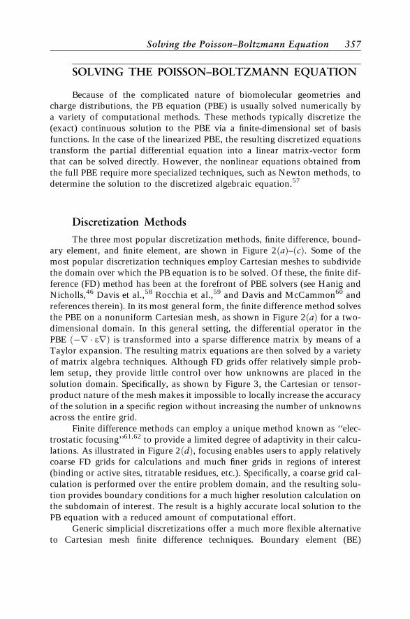
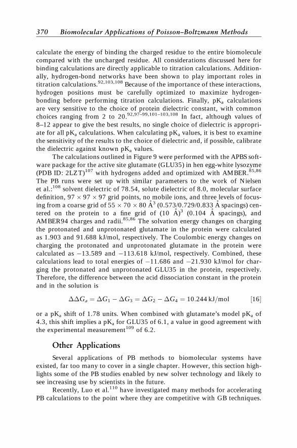
The three most popular discretization methods, finite difference, bound-ary element, and finite element, are shown in Figure 2ðaÞ–ðcÞ. Some of themost popular discretization techniques employ Cartesian meshes to subdividethe domain over which the PB equation is to be solved. Of these, the finite dif-ference (FD) method has been at the forefront of PBE solvers (see Hanig andNicholls,46 Davis et al.,58 Rocchia et al.,59 and Davis and McCammon60 andreferences therein). In its most general form, the finite difference method solvesthe PBE on a nonuniform Cartesian mesh, as shown in Figure 2ðaÞ for a two-dimensional domain. In this general setting, the differential operator in thePBE ð�r � erÞ is transformed into a sparse difference matrix by means of aTaylor expansion. The resulting matrix equations are then solved by a varietyof matrix algebra techniques. Although FD grids offer relatively simple prob-lem setup, they provide little control over how unknowns are placed in thesolution domain. Specifically, as shown by Figure 3, the Cartesian or tensor-product nature of the mesh makes it impossible to locally increase the accuracyof the solution in a specific region without increasing the number of unknownsacross the entire grid.

Finite difference methods can employ a unique method known as ‘‘elec-trostatic focusing’’61,62 to provide a limited degree of adaptivity in their calcu-lations. As illustrated in Figure 2ðdÞ, focusing enables users to apply relativelycoarse FD grids for calculations and much finer grids in regions of interest(binding or active sites, titratable residues, etc.). Specifically, a coarse grid cal-culation is performed over the entire problem domain, and the resulting solu-tion provides boundary conditions for a much higher resolution calculation onthe subdomain of interest. The result is a highly accurate local solution to thePB equation with a reduced amount of computational effort.

Generic simplicial discretizations offer a much more flexible alternativeto Cartesian mesh finite difference techniques. Boundary element (BE)

Solving the Poisson–Boltzmann Equation 357

Figure 3 Adaptive refinement for finite different (left) and finite element (right)methods. Shading denotes successive levels of refinement. See color insert.

Figure 2 Popular discretization schemes for numerical solution of the Poisson–Boltzmann equation. The solid black line and circles denote a model protein; other linesdenote the mesh on which the system is discretized. ðaÞ Finite difference. ðbÞ Boundaryelement. ðcÞ Finite Element. ðdÞ Focusing on finite difference grids. See color insert.


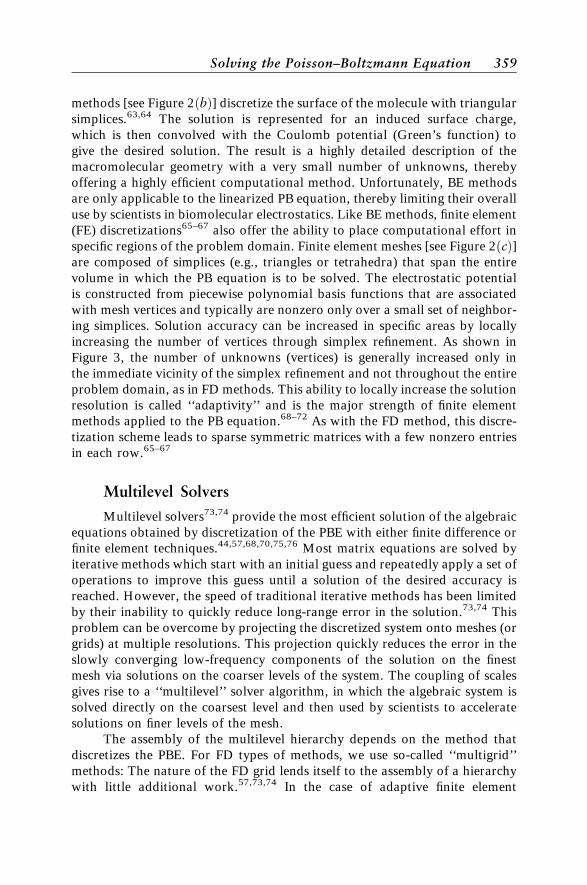
methods [see Figure 2ðbÞ] discretize the surface of the molecule with triangularsimplices.63,64 The solution is represented for an induced surface charge,which is then convolved with the Coulomb potential (Green’s function) togive the desired solution. The result is a highly detailed description of themacromolecular geometry with a very small number of unknowns, therebyoffering a highly efficient computational method. Unfortunately, BE methodsare only applicable to the linearized PB equation, thereby limiting their overalluse by scientists in biomolecular electrostatics. Like BE methods, finite element(FE) discretizations65–67 also offer the ability to place computational effort inspecific regions of the problem domain. Finite element meshes [see Figure 2ðcÞ]are composed of simplices (e.g., triangles or tetrahedra) that span the entirevolume in which the PB equation is to be solved. The electrostatic potentialis constructed from piecewise polynomial basis functions that are associatedwith mesh vertices and typically are nonzero only over a small set of neighbor-ing simplices. Solution accuracy can be increased in specific areas by locallyincreasing the number of vertices through simplex refinement. As shown inFigure 3, the number of unknowns (vertices) is generally increased only inthe immediate vicinity of the simplex refinement and not throughout the entireproblem domain, as in FD methods. This ability to locally increase the solutionresolution is called ‘‘adaptivity’’ and is the major strength of finite elementmethods applied to the PB equation.68–72 As with the FD method, this discre-tization scheme leads to sparse symmetric matrices with a few nonzero entriesin each row.65–67

Multilevel Solvers

Multilevel solvers73,74 provide the most efficient solution of the algebraicequations obtained by discretization of the PBE with either finite difference orfinite element techniques.44,57,68,70,75,76 Most matrix equations are solved byiterative methods which start with an initial guess and repeatedly apply a set ofoperations to improve this guess until a solution of the desired accuracy isreached. However, the speed of traditional iterative methods has been limitedby their inability to quickly reduce long-range error in the solution.73,74 Thisproblem can be overcome by projecting the discretized system onto meshes (orgrids) at multiple resolutions. This projection quickly reduces the error in theslowly converging low-frequency components of the solution on the finestmesh via solutions on the coarser levels of the system. The coupling of scalesgives rise to a ‘‘multilevel’’ solver algorithm, in which the algebraic system issolved directly on the coarsest level and then used by scientists to acceleratesolutions on finer levels of the mesh.

The assembly of the multilevel hierarchy depends on the method thatdiscretizes the PBE. For FD types of methods, we use so-called ‘‘multigrid’’methods: The nature of the FD grid lends itself to the assembly of a hierarchywith little additional work.57,73,74 In the case of adaptive finite element

Solving the Poisson–Boltzmann Equation 359

discretizations, ‘‘algebraic multigrid’’ methods70,75 are employed. For FEmeshes, the most natural multiscale representation is constructed by refine-ment of an initial mesh that typically constitutes the coarsest level of the hier-archy (see Figure 3).

Parallel Methods

Regardless of the scalability of the numerical algorithm that solves thePB equation, some systems are simply too large to be solved sequentially(i.e., on one processor). For example, although small- to medium-sized proteinsystems (100–1000 residues) are amenable to sequential calculations, anincreasing interest exists in macromolecular assemblages with tens to hun-dreds of thousands of residues (e.g., microtubules, entire viral capsids, ribo-somes, polymerases, etc.). Studies of these large systems are not feasible onmost sequential platforms; instead, they require multiprocessor computingplatforms to solve the PB equation in a parallel fashion. However, recent pro-gress in parallel solution methods75,77 has extended the applicability of PBtheory to these large biomolecular systems. Parallel methods have been appliedto both finite element70 and finite difference76 discretizations of the PBequation.

Software for Computational Electrostatics

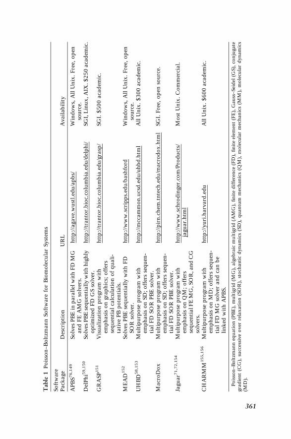
Table 1 presents a list of the major software that currently solves thePoisson–Boltzmann equation for biomolecular systems. A variety of such pro-grams exist, ranging from multipurpose computational biology packages (e.g.,CHARMM, Jaguar, UHBD, and MacroDox) to specialized PB solvers (e.g.,APBS, MEAD, and DelPhi).

In addition to the traditional ‘‘stand-alone’’ software packages listed inTable 1, web-based services are becoming available for solving the PB equa-tion. Such services have the advantage of removing the troublesome detailsof software installation from the user. Quite often, web services also simplifyand/or automate the process of setting up calculations. One example of suchweb-based packages is the APBS Web Portal (https://gridport.npaci.edu/apbs/),a service for preparing, submitting, and organizing electrostatics calculationson supercomputing platforms. This web portal is aimed at quantitative elec-trostatics calculations and currently does not offer substantial analysis orvisualization options. On the other hand, the GRASP (http://trantor.bioc.columbia.edu/) web service supports qualitative electrostatics calculationswith extensive visualization capabilities. GRASP allows users to easily calcu-late and visualize electrostatic potentials and other properties with uploadedstructures or PDB entries. Finally, the MolSurfer (http://projects.villa-bosch.de/dbase/molsurfer/) service also offers qualitative analysis of the electrostaticproperties of biomolecules with specific attention to surface-based quantities.


Table

1Pois

son–B

olt

zmann

Soft

ware

for

Bio

mole

cula

rSyst

ems

Soft

ware

Pack

age

Des

crip

tion

UR

LA

vail

abil

ity

APB

S76,1

49

Solv

esPB

Ein

para

llel

wit

hFD

MG

and

FE

AM

Gso

lver

s.htt

p:/

/agave.

wust

l.ed

u/a

pbs/

Win

dow

s,A

llU

nix

.Fre

e,open

sourc

e.D

elPhi5

9,1

50

Solv

esPB

Ese

quen

tiall

yw

ith

hig

hly

opti

miz

edFD

GS

solv

er.

htt

p:/

/tra

nto

r.bio

c.co

lum

bia

.edu/d

elphi/

SG

I,L

inux,A

IX.$250

aca

dem

ic.

GR

ASP

151

Vis

uali

zati

on

pro

gra

mw

ith

emphasi

son

gra

phic

s;off

ers

sequen

tial

calc

ula

tion

of

quali

-ta

tive

PB

pote

nti

als

.

htt

p:/

/tra

nto

r.bio

c.co

lum

bia

.edu/g

rasp

/SG

I.$500

aca

dem

ic.

ME

AD

152

Solv

esPB

Ese

quen

tiall

yw

ith

FD

SO

Rso

lver

.htt

p:/

/ww

w.s

crip

ps.

edu/b

ash

ford

Win

dow

s,A

llU

nix

.Fre

e,open

sourc

e.U

HB

D58,1

53

Mult

ipurp

ose

pro

gra

mw

ith

emphasi

son

SD

;off

ers

sequen

-ti

al

FD

SO

RPB

Eso

lver

.

htt

p:/

/mcc

am

mon.u

csd.e

du/u

hbd.h

tml

All

Unix

.$300

aca

dem

ic.

Macr

oD

ox

Mult

ipurp

ose

pro

gra

mw

ith

emphasi

son

SD

;off

ers

sequen

-ti

al

FD

SO

RPB

Eso

lver

.

htt

p:/

/pir

n.c

hem

.tnte

ch.e

du/m

acr

odox.h

tml

SG

I.Fre

e,open

sourc

e.

Jaguar7

1,7

2,1

54

Mult

ipurp

ose

pro

gra

mw

ith

emphasi

son

QM

;off

ers

sequen

tialF

EM

G,S

OR

,and

CG

solv

ers.

htt

p:/

/ww

w.s

chro

din

ger

.com

/Pro

duct

s/ja

guar.

htm

lM

ost

Unix

.C

om

mer

cial.

CH

AR

MM

155,1

56

Mult

ipurp

ose

pro

gra

mw

ith

emphasi

son

MD

;off

ers

sequen

-ti

al

FD

MG

solv

erand

can

be

linked

wit

hA

PB

S.

htt

p:/

/yuri

.harv

ard

.edu

All

Unix

.$600

aca

dem

ic.

Pois

son–B

olt

zmann

equati

on

(PB

E),

mult

igri

d(M

G),

alg

ebra

icm

ult

igri

d(A

MG

),finit

edif

fere

nce

(FD

),finit

eel

emen

t(F

E),

Gau

ss–Sei

del

(GS),

conju

gate

gra

die

nt

(CG

),su

cces

sive

over

rela

xati

on

(SO

R),

stoch

ast

icdynam

ics

(SD

),quantu

mm

echanic

s(Q

M),

mole

cula

rm

echanic

s(M

M),

mole

cula

rdynam

ics

(MD

).

361

APPLYING POISSON–BOLTZMANN METHODS

The purpose of this section is to illustrate the application of PB methodsto various molecular and biomolecular problems. Where feasible, the pro-blems are described in sufficient detail to allow readers to further investigatethese systems with any of the software packages listed in Table 1. Addition-ally, these examples are included in the APBS software package distribution(http://agave.wustl.edu/apbs/)76 and are freely available for download.

Solvation Free Energies

One of the simplest PB calculations is the solvation-free energy. Thesetypes of problems consider the energy of transferring a solute from a uniformdielectric continuum (of permittivity ep) to an inhomogeneous medium withbulk dielectric ðesÞ equal to that of the solvent (see Figure 4). To evaluate sol-vation energies, two PB calculations are performed: (1) Calculate the energyG1 of the system with a constant dielectric ep, and (2) calculate the energyG2 of the system with solute dielectric ep and solvent dielectric es. The solva-tion energy is then the difference of these two calculations: �Gsolv ¼ G2 � G1.One aspect of this procedure that should immediately be questioned is Step (1).If we are using a homogeneous dielectric, why do we need to perform a numer-ical PB calculation; why not just use Coulomb’s law? The reasons for thisapparently superfluous calculation are twofold. First, PB energies include‘‘self-interaction’’ terms, i.e., the energy of a charge distribution interactingwith itself. For point charges, an exact solution to the PB equation shouldgive infinite self-interaction terms. The finite (but large!) nature of these

Figure 4 Schematic of a solvation energy calculation. The initial state treats the solute ina homogeneous dielectric material with both solvent and solute dielectric coefficients setto solute value ep. The final state involves an inhomogeneous dielectric coefficient withsolute value ep and bulk solvent value es.


components for numerical solutions is caused by the finite discretizationapplied in FD and FE methods. Second, these terms are extremely sensitiveto the discretization scheme that solves the PB equation. In other words, smallchanges in grid spacing or the location of these charges on the grid gives rise tovery large changes in the self-interaction terms. For these reasons, self-interac-tions are always removed from PB calculations—energies obtained from a sin-gle PB calculation are meaningless.

The Born ion28 is the simplest model of solvation: It considers the solva-tion energy of a spherical, nonpolarizable ðep ¼ 1Þ solute of radius R with asingle point charge of magnitude z at its center. In this case, an analyticalexpression is available for the solvation energy:

�GBorn ¼ � z2e2c

8pe0R1 � 1

ee

� �½9

This simple model reproduces many of the basic characteristics we wouldexpect from ion solvation; the solvation energy decreases with the ion size,increases with the charge magnitude, and is roughly independent of the chargesign. In fact, the Born model performs very well at describing the solvationproperties of low charge-density ions (large and/or monovalent) but fails forhigher charge systems where dielectric saturation and solvent electrostrictionbecome significant.

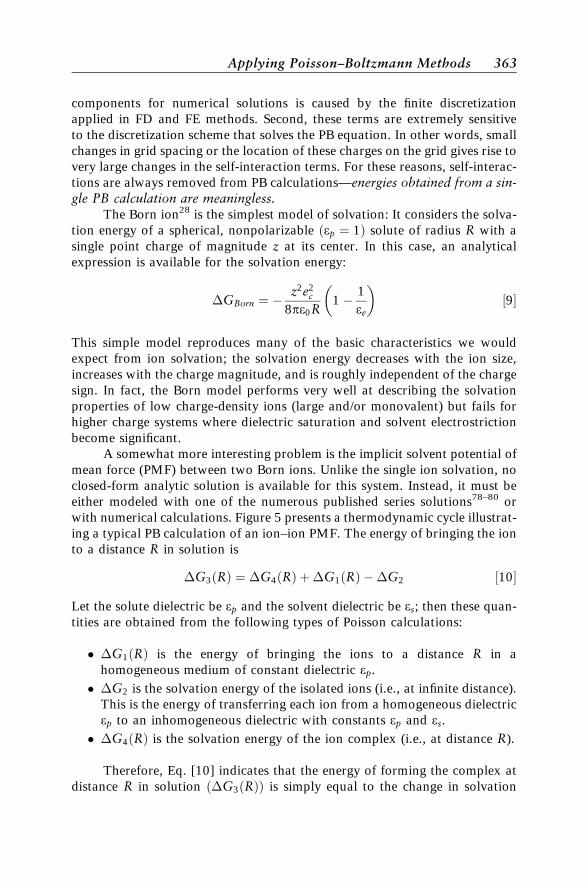
A somewhat more interesting problem is the implicit solvent potential ofmean force (PMF) between two Born ions. Unlike the single ion solvation, noclosed-form analytic solution is available for this system. Instead, it must beeither modeled with one of the numerous published series solutions78–80 orwith numerical calculations. Figure 5 presents a thermodynamic cycle illustrat-ing a typical PB calculation of an ion–ion PMF. The energy of bringing the ionto a distance R in solution is

�G3ðRÞ ¼ �G4ðRÞ þ�G1ðRÞ ��G2 ½10

Let the solute dielectric be ep and the solvent dielectric be es; then these quan-tities are obtained from the following types of Poisson calculations:

� �G1ðRÞ is the energy of bringing the ions to a distance R in ahomogeneous medium of constant dielectric ep.

� �G2 is the solvation energy of the isolated ions (i.e., at infinite distance).This is the energy of transferring each ion from a homogeneous dielectricep to an inhomogeneous dielectric with constants ep and es.

� �G4ðRÞ is the solvation energy of the ion complex (i.e., at distance R).

Therefore, Eq. [10] indicates that the energy of forming the complex atdistance R in solution ð�G3ðRÞÞ is simply equal to the change in solvation

Applying Poisson–Boltzmann Methods 363

energy ð�G4ðRÞ ��G2Þ—or desolvation energy—plus the Coulombic inter-action energy of the solutes in a homogeneous dielectric ð�G1ðRÞÞ.

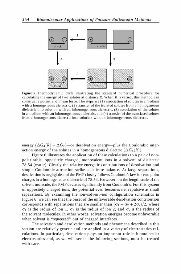
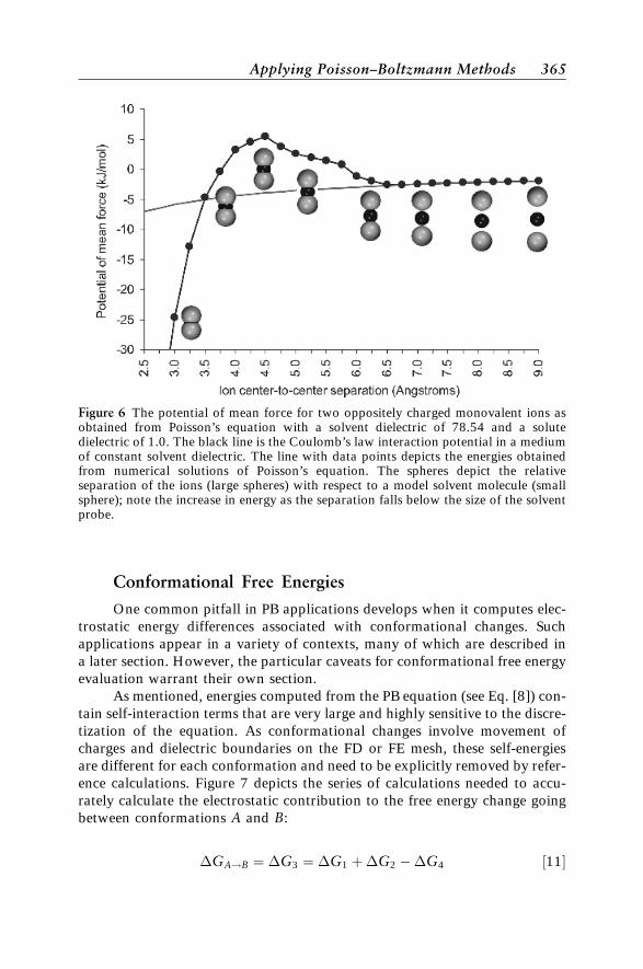
Figure 6 illustrates the application of these calculations to a pair of non-polarizable, oppositely charged, monovalent ions in a solvent of dielectric78.54 (water). Clearly the relative energetic contributions of desolvation andsimple Coulombic attraction strike a delicate balance. At large separations,desolvation is negligible and the PMF closely follows Coulomb’s law for two pointcharges in a homogeneous dielectric of 78.54. However, on the length scale of thesolvent molecule, the PMF deviates significantly from Coulomb’s. For this systemof oppositely charged ions, the potential even becomes net repulsive at smallseparations. By examining the ion–solvent–ion configuration schematics inFigure 6, we can see that the onset of the unfavorable desolvation contributioncorresponds with separations that are smaller than ðs1 þ s2 þ 2ssÞ=2, wheres1 is the radius of ion 1, s2 is the radius of ion 2, and ss is the radius ofthe solvent molecules. In other words, solvation energies become unfavorablewhen solvent is ‘‘squeezed’’ out of charged interfaces.

The solvation and desolvation methods and phenomena described in thissection are relatively generic and are applied in a variety of electrostatics cal-culations. In particular, desolvation plays an important role in biomolecularelectrostatics and, as we will see in the following sections, must be treatedwith care.

Figure 5 Thermodynamic cycle illustrating the standard numerical procedure forcalculating the energy of two solutes at distance R. When R is varied, this method canconstruct a potential of mean force. The steps are (1) association of solutes in a mediumwith a homogeneous dielectric, (2) transfer of the isolated solutes from a homogeneousdielectric into solution with an inhomogeneous dielectric, (3) association of the solutesin a medium with an inhomogeneous dielectric, and (4) transfer of the associated solutesfrom a homogeneous dielectric into solution with an inhomogeneous dielectric.


Conformational Free Energies

One common pitfall in PB applications develops when it computes elec-trostatic energy differences associated with conformational changes. Suchapplications appear in a variety of contexts, many of which are described ina later section. However, the particular caveats for conformational free energyevaluation warrant their own section.

As mentioned, energies computed from the PB equation (see Eq. [8]) con-tain self-interaction terms that are very large and highly sensitive to the discre-tization of the equation. As conformational changes involve movement ofcharges and dielectric boundaries on the FD or FE mesh, these self-energiesare different for each conformation and need to be explicitly removed by refer-ence calculations. Figure 7 depicts the series of calculations needed to accu-rately calculate the electrostatic contribution to the free energy change goingbetween conformations A and B:

�GA!B ¼ �G3 ¼ �G1 þ�G2 ��G4 ½11

Figure 6 The potential of mean force for two oppositely charged monovalent ions asobtained from Poisson’s equation with a solvent dielectric of 78.54 and a solutedielectric of 1.0. The black line is the Coulomb’s law interaction potential in a mediumof constant solvent dielectric. The line with data points depicts the energies obtainedfrom numerical solutions of Poisson’s equation. The spheres depict the relativeseparation of the ions (large spheres) with respect to a model solvent molecule (smallsphere); note the increase in energy as the separation falls below the size of the solventprobe.


The self-energies are explicitly removed in the calculation of the change in sol-vation energy ð�G4 ��G2Þ association with the conformational change. Aswith the ion–ion PMF example, solvation energies strive to expose polar sur-faces and generally oppose the association of any charged molecular surfaces.For the toy example shown in Figure 7, polar solvation forces would beexpected to favor conformation A. Finally, the remaining term in Eq. [11]ð�G1Þ denotes the usual Coulombic contribution to the electrostatic energy;it is the change in internal electrostatic energy (for a homogeneous dielectric ofep) caused by the conformational change.

Unlike the ion–ion PMF case, substantial apolar surface area is oftenburied during biomolecular conformational changes and/or complex forma-tion. Therefore, we must also consider the apolar solvation energies discussedin a previous section. For the current example, a constant apolar coefficientmethod would provide an additional term for the conformational change:

�Gapolar ¼ g�A ½12

where g is the apolar coefficient and �A is the difference in surface area causedby the conformational change. As g � 0, this term favors the burial of mole-cular surfaces and therefore counteracts the polar solvation forces. In practice,apolar and polar energy terms strike a tenuous balance in stabilizing biomole-cular complexes and conformations.

Figure 7 Thermodynamic cycle illustrating the standard numerical procedure forcalculating the electrostatic energy of a conformational change in a molecule. The stepsare (1) conformational change in a homogeneous dielectric, (2) transfer of conformationB from a homogeneous dielectric into solution with an inhomogeneous dielectric, (3)conformational change in an inhomogeneous dielectric, and (4) transfer of conforma-tion A from a homogeneous dielectric into solution with an inhomogeneous dielectric.


Binding Free Energies

The calculation of binding free energies is arguably the most commonapplication of PB methods. As described earlier, PB methods provide the elec-trostatic energies and are often supplemented with additional terms represent-ing apolar and other interactions. These calculations are performed on a widevariety of complexes ranging from small molecule–protein interactions81 toprotein–membrane interactions82 and the energy of supramolecular assem-bly.83

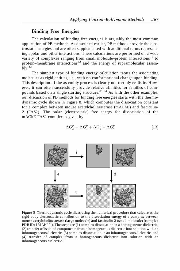
The simplest type of binding energy calculation treats the associatingmolecules as rigid entities, i.e., with no conformational change upon binding.This description of the assembly process is clearly not terribly realistic. How-ever, it can often successfully provide relative affinities for families of com-pounds based on a single starting structure.81,84 As with the other examples,our discussion of PB methods for binding free energies starts with the thermo-dynamic cycle shown in Figure 8, which computes the dissociation constantfor a complex between mouse acetylcholinesterase (mAChE) and fasciculin-2 (FAS2). The polar (electrostatic) free energy for dissociation of themAChE-FAS2 complex is given by

�Gp3 ¼ �Gp

1 þ�Gp2 ��Gp

4 ½13

Figure 8 Thermodynamic cycle illustrating the numerical procedure that calculates therigid-body electrostatic contribution to the dissociation energy of a complex betweenmouse acetylcholinesterase (large molecule) and fasciculin-2 (small molecule) (complexPDB ID: 1MAH157). The steps are (1) complex dissociation in a homogeneous dielectric,(2) transfer of isolated components from a homogeneous dielectric into solution with aninhomogeneous dielectric, (3) complex dissociation in an inhomogeneous dielectric, and(4) transfer of complex from a homogeneous dielectric into solution with aninhomogeneous dielectric.


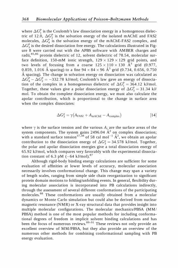
where �Gp1 is the Coulomb’s law dissociation energy in a homogenous dielec-

tric of 12.0, �Gp2 is the solvation energy of the isolated mAChE and FAS2

molecules, �Gp4 is the solvation energy of the mAChE-FAS2 complex, and

�Gp3 is the desired dissociation free energy. The calculations illustrated in Fig-

ure 8 were carried out with the APBS software with AMBER charges andradii,85,86 protein dielectric of 12, solvent dielectric of 78.54, molecular sur-face definition, 150-mM ionic strength, 129 � 129 � 129 grid points, andtwo levels of focusing from a coarse 125 � 110 � 130 A3 grid (0.977,0.859, 1.016 A spacing) to a fine 94 � 84 � 96 A3 grid (0.734, 0.656, 0.750A spacing). The change in solvation energy on dissociation was calculated as�Gp

4 ��Gp2 ¼ �332:78 kJ/mol; Coulomb’s law gave an energy of dissocia-

tion of the complex in a homogeneous dielectric of �Gp1 ¼ 364:12 kJ/mol.

Together, these values give a polar dissociation energy of �Gp3 ¼ 31:34 kJ/

mol. To obtain the complete dissociation energy, we must also calculate theapolar contribution, which is proportional to the change in surface areawhen the complex dissociates:

�Ga3 ¼ g AFAS2 þ AmAChE � Acomplex

� �½14

where g is the surface tension and the various Ai are the surface areas of thesystem components. The system gains 2496.04 A2 on complex dissociation;with a standard surface tension37,38 of 58 cal mol�1 A2, we obtain an apolarcontribution to the dissociation energy of �Ga

3 ¼ 34:578 kJ/mol. Together,the polar and apolar dissociation energies give a total dissociation energy of65.92 kJ/mol, which compares very favorably with the experimental dissocia-tion constant of 6.3 pM (�64 kJ/mol).87

Although rigid-body binding energy calculations are sufficient for someevaluation of affinities at lower levels of accuracy, molecular associationnecessarily involves conformational change. This change may span a varietyof length scales, ranging from simple side chain reorganization to significantprotein domain motions to folding/unfolding events. In general, flexibility dur-ing molecular association is incorporated into PB calculations indirectly,through the assessment of several different conformations of the participatingmolecules.88 These conformations are usually obtained from a moleculardynamics or Monte Carlo simulation but could also be derived from nuclearmagnetic resonance (NMR) or X-ray structural data that provides insight intomultiple molecular configurations. The molecular mechanics/PBSA (MM/PBSA) method is one of the most popular methods for including conforma-tional degrees of freedom in implicit solvent binding calculations and hasbeen the focus of numerous reviews.89–91 These reviews not only provide anexcellent overview of MM/PBSA, but they also provide an overview of thenumerous other methods for combining conformational sampling with PBenergy evaluation.


Titration Calculations

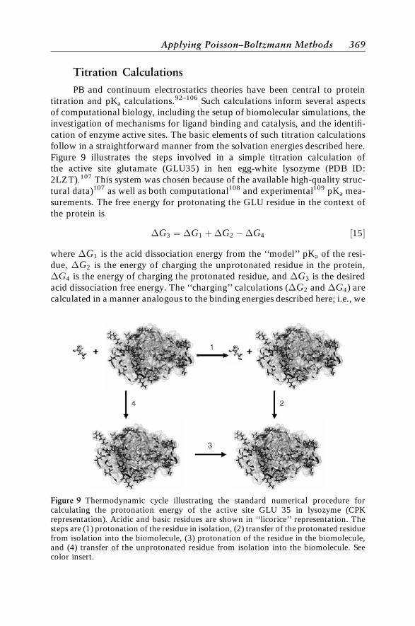
PB and continuum electrostatics theories have been central to proteintitration and pKa calculations.92–106 Such calculations inform several aspectsof computational biology, including the setup of biomolecular simulations, theinvestigation of mechanisms for ligand binding and catalysis, and the identifi-cation of enzyme active sites. The basic elements of such titration calculationsfollow in a straightforward manner from the solvation energies described here.Figure 9 illustrates the steps involved in a simple titration calculation ofthe active site glutamate (GLU35) in hen egg-white lysozyme (PDB ID:2LZT).107 This system was chosen because of the available high-quality struc-tural data)107 as well as both computational108 and experimental109 pKa mea-surements. The free energy for protonating the GLU residue in the context ofthe protein is

�G3 ¼ �G1 þ�G2 ��G4 ½15

where �G1 is the acid dissociation energy from the ‘‘model’’ pKa of the resi-due, �G2 is the energy of charging the unprotonated residue in the protein,�G4 is the energy of charging the protonated residue, and �G3 is the desiredacid dissociation free energy. The ‘‘charging’’ calculations (�G2 and �G4) arecalculated in a manner analogous to the binding energies described here; i.e., we

Figure 9 Thermodynamic cycle illustrating the standard numerical procedure forcalculating the protonation energy of the active site GLU 35 in lysozyme (CPKrepresentation). Acidic and basic residues are shown in ‘‘licorice’’ representation. Thesteps are (1) protonation of the residue in isolation, (2) transfer of the protonated residuefrom isolation into the biomolecule, (3) protonation of the residue in the biomolecule,and (4) transfer of the unprotonated residue from isolation into the biomolecule. Seecolor insert.


calculate the energy of binding the charged residue to the entire biomoleculecompared with the uncharged residue. All considerations discussed here forbinding calculations are directly applicable to titration calculations. Addition-ally, hydrogen-bond networks have been shown to play important roles intitration calculations.92,103,108 Because of the importance of these interactions,hydrogen positions must be carefully optimized to maximize hydrogen-bonding before performing titration calculations. Finally, pKa calculationsare very sensitive to the choice of protein dielectric constant, with commonchoices ranging from 2 to 20.92,97–99,101–103,108 In fact, although values of8–12 appear to give the best results, no single choice of dielectric is appropri-ate for all pKa calculations. When calculating pKa values, it is best to examinethe sensitivity of the results to the choice of dielectric and, if possible, calibratethe dielectric against known pKa values.

The calculations outlined in Figure 9 were performed with the APBS soft-ware package for the active site glutamate (GLU35) in hen egg-white lysozyme(PDB ID: 2LZT)107 with hydrogens added and optimized with AMBER.85,86

The PB runs were set up with similar parameters to the work of Nielsenet al.:108 solvent dielectric of 78.54, solute dielectric of 8.0, molecular surfacedefinition, 97 � 97 � 97 grid points, no mobile ions, and three levels of focus-ing from a coarse grid of 55 � 70 � 80 A3 (0.573/0.729/0.833 A spacings) cen-tered on the protein to a fine grid of (10 A)3 (0.104 A spacings), andAMBER94 charges and radii.85,86 The solvation energy changes on chargingthe protonated and unprotonated glutamate in the protein were calculatedas 1.903 and 91.688 kJ/mol, respectively. The Coulombic energy changes oncharging the protonated and unprotonated glutamate in the protein werecalculated as �13.589 and �113.618 kJ/mol, respectively. Combined, thesecalculations lead to total energies of �11.686 and �21.930 kJ/mol for char-ging the protonated and unprotonated GLU35 in the protein, respectively.Therefore, the difference between the acid dissociation constant in the proteinand in the solution is

��Ga ¼ �G1 ��G3 ¼ �G2 ��G4 ¼ 10:244 kJ=mol ½16

or a pKa shift of 1.78 units. When combined with glutamate’s model pKa of4.3, this shift implies a pKa for GLU35 of 6.1, a value in good agreement withthe experimental measurement109 of 6.2.

Other Applications

Several applications of PB methods to biomolecular systems haveexisted, far too many to cover in a single chapter. However, this section high-lights some of the PB studies enabled by new solver technology and likely tosee increasing use by scientists in the future.

Recently, Luo et al.110 have investigated many methods for acceleratingPB calculations to the point where they are competitive with GB techniques.


Encouragingly, the acceleration methods described by Luo et al. are applicableto many software packages and could improve many PB solvers. Althoughmany applications can benefit from faster PB methods, perhaps the most pro-found advantage will be in the realm of stochastic dynamics simulations111 byenabling the efficient implicit solvent simulations of protein dynamics at thePB level of electrostatics theory.

Additionally, some recent efforts have been made to pursue more ‘‘infor-matics’’-based approaches to the interpretation of electrostatic properties.Much of this work includes identification of functionally relevant residues inproteins by looking at electrostatic destabilization of conserved residues,112

highly shifted pKa values,93 clusters of charged residues,113 and protein-membraneinteractions.82,114–118 Other research has focused on comparisons of electro-static potential between biomolecules, including analyses of polar and chargegroup complementarity at biomolecular interfaces119–124 and similarity ofelectrostatic potentials both at molecular surfaces82,114–117,123–132 and inthree-dimensional space.128,133–143 Although the past characterization of elec-trostatic properties of biomolecules has provided insight into a variety of bio-molecular properties, previous applications only focused on a few quantitativemeasures of electrostatic properties and limited their studies to relatively fewbiomolecules. However, with the rapid growth of biomolecular structures elu-cidated by structural genomics efforts144,145 and the burgeoning interest inunderstanding biomolecular interactions in a proteomics context, high-throughput tools to facilitate the analysis of electrostatic properties acrossthousands of biomolecular structures will become increasingly important.

Finally, with the advent of new parallel solution methods for the PBequation70,76 and the increase in sequential computer capabilities, PB methodsare being applied to increasingly larger systems. Recent examples of particu-larly large-scale PB calculations include the study of microtubule structure andstability,83 binding calculations of aminoglycoside antibiotics to the smallribosomal subunit,84 modeling of RNA organization inside viral capsids,146

and examination of electrostatic interactions in protein-membrane interac-tions.82,114–117 Given the rate of increase in computational capabilities, orga-nelle-scale calculations appear feasible in the not-too-distant future. However,it is easy to get carried away with the scale of calculations possible with newmethods and technology; we should always consider the fundamental limita-tions of continuum approaches and make sure the equations we used in themodel are appropriate to the systems under consideration.

CONCLUSIONS

An understanding of electrostatic interactions is essential for the study ofbiomolecular processes. The structures of proteins and other biopolymers arebeing determined at an increasing rate through structural genomics and other

Conclusions 371

efforts, whereas specific linkages of these biopolymers in cellular pathways orsupramolecular assemblages are being detected by genetic and proteomic stu-dies. To integrate this information in physical models for drug discovery orother applications requires the ability to evaluate the energetic interactionswithin and between biopolymers. Among the various components of molecu-lar energetics, the electrostatic interactions are of special importance becauseof the long range of these interactions and the substantial charges of typicalbiopolymer components.

In this chapter, we have covered some of the basic elements of the Pois-son–Boltzmann implicit solvent description of biomolecular electrostatics.Specifically, we have focused on the application of these methods to basic pro-blems in computational biology. The discussion presented here is necessarilyincomplete—electrostatics is a very broad field and continually changing.For additional background and more in-depth discussions of some of the prin-ciples and limitations of continuum electrostatics, interested readers should seethe general continuum electrostatics texts by Jackson47 and Landau et al.,147

the electrochemistry text of Bockris et al.,16 the colloid theory treatise byVerwey and Overbeek,148 and the fantastic collection of condensed matterelectrostatics articles assembled by Holm et al.13

ACKNOWLEDGMENTS

Support for this work was provided by the Washington University in St. Louis, NationalPartnership for Advanced Computational Infrastructure, NIH Grant GM069702, and an AlfredP. Sloan Foundation Research Fellowship.

REFERENCES

1. J. M. Wang, P. Cieplak, and P. A. Kollman, J. Comput. Chem., 21, 1049 (2000). How WellDoes a Restrained Electrostatic Potential (RESP) Model Perform in Calculating Conforma-tional Energies of Organic and Biological Molecules?

2. C. I. Bayly, P. Cieplak, W. D. Cornell, and P. A. Kollman, J. Phys. Chem., 97, 10269 (1993). AWell-Behaved Electrostatic Potential Based Method Using Charge Restraints for DerivingAtomic Charges—the RESP Model.

3. A. Grossfield, P. Ren, and J. W. Ponder, J. Am. Chem. Soc., 125, 15671 (2003). Ion SolvationThermodynamics from Simulation with a Polarizable Force Field.

4. P. Ren and J. W. Ponder, J. Comput. Chem., 23, 1497 (2002). Consistent Treatment of Inter-and Intramolecular Polarization in Molecular Mechanics Calculations.

5. A. D. MacKerell, Jr. in Computational Biochemistry and Biophysics, O. M. Becker, A. D. J.MacKerell, B. Roux, and M. Watanabe, Eds., Marcel-Dekker: New York, 2001, p. 7.Atomistic Models and Force Fields.

6. A. R. Leach, Molecular Modelling: Principles and Applications, Prentice Hall, Harlow,England, 2001.

7. T. Schlick, Molecular Modeling and Simulation: An Interdisciplinary Guide, Springer-Verlag,New York, 2002.


8. G. Lamm, in Reviews in Computational Chemistry, Vol. 19, K. B. Lipkowitz, R. Larter, andT. R. Cundari, Eds., Wiley, Hoboken, New Jersey, 2003, pp. 147–365. The Poisson-Boltzmann Equation.

9. W. Nonner, D. Gillespe, D. Henderson, and D. Eisenberg, J. Phys. Chem. B, 105, 6427 (2001).Ion Accumulation in a Biological Calcium Channel: Effects of Solvent and Confining Pressure.

10. S. M. Bhattacharyya, Z.-G. Wang, and A. H. Zewail, J. Phys. Chem. B, 107, 13218 (2003).Dynamics of Water Near a Protein Surface.

11. F. Figueirido, G. S. Delbuono, and R. M. Levy, Biophys. Chem., 51, 235 (1994). MolecularMechanics and Electrostatic Effects.

12. J.-H. Lin, N. A. Baker, and J. A. McCammon, Biophys. J., 83, 1374 (2002). Bridging theImplicit and Explicit Solvent Approaches for Membrane Electrostatics.

13. C. Holm, P. Kekicheff, and R. Podgornik, Eds., Electrostatic Effects in Soft Matterand Biophysics, NATO Science Series. Vol. 46, Kluwer Academic Publishers, Boston,Massachusetts, 2001.

14. T. Simonson, Curr. Opin. Struct. Biol., 11, 243 (2001). Macromolecular Electrostatics:Continuum Models and Their Growing Pains.

15. B. Roux, in Computational Biochemistry and Biophysics, O. M. Becker, A. D. MacKerell, Jr.,B. Roux, and M. Watanabe, Eds., Marcel Dekker, New York, 2001, p. 133. Implicit SolventModels.

16. J. O. Bockris, and A. K. N. Reddy, Modern Electrochemistry: Ionics, Plenum Press, New York,1998.

17. A. D. MacKerell, Jr. and L. Nilsson, in Computational Biochemistry and Biophysics, O. M.Becker, A. D. MacKerell, Jr., B. Roux, and M. Watanabe, Eds., Marcel Dekker: New York,2001, pp. 441–463. Nucleic Acid Simulations.

18. G. Hummer, L. R. Pratt, and A. E. Garcia, J. Chem. Phys., 107, 9275 (1997). Ion Sizes andFinite-size Corrections for Ionic-solvation Free Energies.

19. I. G. Tironi, R. Sperb, P. E. Smith, and W. F. van Gunsteren, J. Chem. Phys., 102, 5451 (1995).A Generalized Reaction Field Method for Molecular Dynamics Simulations.

20. N. A. Baker, P. H. Hunenberger, and J. A. McCammon, J. Chem. Phys., 110, 10679 (1999).Polarization Around an Ion in a Dielectric Continuum with Truncated Electrostatic Inter-actions.

21. H. S. Ashbaugh and M. E. Paulaitis, J. Phys. Chem. B, 102, 5029 (1998). A Molecular/Continuum Thermodynamic Model of Hydration.

22. M. Schaefer and M. Karplus, J. Phys. Chem., 100, 1578 (1996). A Comprehensive AnalyticalTreatment of Continuum Electrostatics.

23. W. C. Still, A. Tempczyk, R. C. Hawley, and T. Hendrickson, J. Am. Chem. Soc., 112, 6127(1990). Semianalytical Treatment of Solvation for Molecular Mechanics andDynamics.

24. B. N. Dominy and C. L. Brooks III, J. Phys. Chem. B, 103, 3765 (1999). Development of aGeneralized Born Model Parameterization for Proteins and Nucleic Acids.

25. D. Bashford and D. A. Case, Annu. Rev. Phys. Chem., 51, 129 (2000). Generalized BornModels of Macromolecular Solvation Effects.

26. K. Osapay, W. S. Young, D. Bashford, C. L. Brooks III, and D. A. Case, J. Phys. Chem., 100,2698 (1996). Dielectric Continuum Models for Hydration Effects on Peptide Conforma-tional Transitions.

27. A. Onufriev, D. A. Case, and D. Bashford, J. Comput. Chem., 23, 1297 (2002). Effective BornRadii in the Generalized Born Approximation: The Importance of Being Perfect.

28. M. Born, Z. Phys., 1, 45 (1920). Volumen und Hydratationswarme der Ionen.

29. L. David, R. Luo, and M. K. Gilson, J. Comput. Chem., 21, 295 (2000). Comparison ofGeneralized Born and Poisson Models: Energetics and Dynamics of HIV Protease.

References 373

30. R. Luo, M. S. Head, J. Moult, and M. K. Gilson, J. Am. Chem. Soc., 120, 6138 (1998). pK(a)Shifts in Small Molecules and HIV Protease: Electrostatics and Conformation.

31. J. A. Given and M. K. Gilson, Proteins: Struct. Funct. Genet., 33, 475 (1998). A HierarchicalMethod for Generating Low-energy Conformers of a Protein-ligand Complex.

32. M. Feig, A. Onufriev, M. S. Lee, W. Im, D. A. Case, and C. L. Brooks III, J. Comput. Chem.,25, 265 (2003). Performance Comparison of Generalized Born and Poisson Methods in theCalculation of Electrostatic Solvation Energies for Protein Structures.

33. J.-P. Hansen and I. R. McDonald, Theory of Simple Liquids, Academic Press, San Diego,California, 2000.

34. F. Stillinger, J. Solution Chem., 2, 141 (1973). Structure in Aqueous Solutions of NonpolarSolutes from the Standpoint of Scaled-particle Theory.

35. R. A. Pierotti, Chem. Rev., 76, 717 (1976). A Scaled Particle Theory of Aqueous andNonaqeous Solutions.

36. T. Simonson and A. T. Brunger, J. Phys. Chem., 98, 4683 (1994). Solvation Free EnergiesEstimated From Macroscopic Continuum Theory: An Accuracy Assessment.

37. K. A. Sharp, A. Nicholls, R. F. Fine, and B. Honig, Science, 252, 106 (1991). Reconciling theMagnitude of the Microscopic and Macroscopic Hydrophobic Effects.

38. C. Chothia, Nature, 248, 338 (1974). Hydrophobic Bonding and Accessible Surface Area inProteins.

39. L. Wesson, and D. Eisenberg, Protein Sci., 1, 227 (1992). Atomic Solvation ParametersApplied to Molecular Dynamics of Proteins in Solution.

40. D. Eisenberg and A. D. McLachlan, Nature, 319, 199 (1986). Solvation Energy in ProteinFolding and Binding.

41. D. M. Huang and D. Chandler, Proc. Nat. Acad. Sci., USA, 97, 8324 (2000). Temperature andLength Scale Dependence of Hydrophobic Effects and their Possible Implications for ProteinFolding.

42. G. Hummer, J. Am. Chem. Soc., 121, 6299 (1999). Hydrophobic Force Field as a MolecularAlternative to Surface-area Models.

43. L. R. Pratt, Annu. Rev. Phys. Chem., 53, 409 (2002). Molecular Theory of HydrophobicEffects: ‘‘She is too Mean to Have Her Name Repeated’’.

44. N. A. Baker and J. A. McCammon, in Structural Bioinformatics, H. Weissig, Ed., Wiley, NewYork, 2002, pp. 427–440. Electrostatic Interactions.

45. M. E. Davis and J. A. McCammon, Chem. Rev., 94, 7684 (1990). Electrostatics in Biomo-lecular Structure and Dynamics.

46. B. Honig and A. Nicholls, Science, 268, 1144 (1995). Classical Electrostatics in Biology andChemistry.

47. J. D. Jackson, Classical Electrodynamics, Wiley, New York, 1975.

48. B. Lee and F. M. Richards, J. Mol. Biol., 55, 379 (1971). The Interpretation of ProteinStructures: Estimation of Static Accessibility.

49. M. L. Connolly, J. Mol. Graph., 11, 139 (1993). The Molecular Surface Package.

50. W. Im, D. Beglov, and B. Roux, Comput. Phys. Commun., 111, 59 (1998). ContinuumSolvation Model: Electrostatic Forces From Numerical Solutions to the Poisson–BoltzmannEquation.

51. C. L. Bajaj, V. Pasucci, R. J. Holt, and A. N. Netravali, Discete Appl. Math., 127, 23 (2003).Dynamic Maintenance and Visualization of Molecular Surfaces.

52. J. A. Grant, B. T. Pickup, and A. Nicholls, J. Comput. Chem., 22, 608 (2001). A SmoothPermittivity Function for Poisson–Boltzmann Solvation Methods.

53. K. A. Sharp and B. Honig, J. Phys. Chem., 94, 7684 (1990). Calculating Total ElectrostaticEnergies with the Nonlinear Poisson–Boltzmann Equation.


54. F. Fogolari and J. M. Briggs, Chem. Phys. Lett., 281, 135 (1997). On the VariationalApproach to Poisson–Boltzmann Free Energies.

55. A. M. Micu, B. Bagheri, A. V. Ilin, L. R. Scott, and B. M. Pettitt, J. Comput. Phys., 136, 263(1997). Numerical Considerations in the Computation of the Electrostatic Free Energy ofInteraction within the Poisson–Boltzmann Theory.

56. M. K. Gilson, M. E. Davis, B. A. Luty, and J. A. McCammon, J. Phys. Chem., 97, 3591 (1993).Computation of Electrostatic Forces on Solvated Molecules using the Poisson–BoltzmannEquation.

57. M. J. Holst and F. Saied, J. Comput. Chem., 16, 337 (1995). Numerical Solution of theNonlinear Poisson–Boltzmann Equation: Developing More Robust and Efficient Methods.

58. M. E. Davis, J. D. Madura, B. A. Luty, and J. A. McCammon, Comput. Phys. Commun., 62,187 (1991). Electrostatics and Diffusion of Molecules in Solution—Simulations with theUniversity-of-Houston-Brownian Dynamics Program.

59. W. Rocchia, S. Sridharan, A. Nicholls, E. Alexov, A. Chiabrera, and B. Honig, J. Comput.Chem., 23, 128 (2002). Rapid Grid-based Construction of the Molecular Surface and the useof Induced Surface Charge to Calculate Reaction Field Energies: Applications to theMolecular Systems and Geometric Objects.

60. M. E. Davis and J. A. McCammon, J. Comput. Chem., 12, 909 (1991). Dielectric BoundarySmoothing in Finite Difference Solutions of the Poisson Equation: An Approach to ImproveAccuracy and Convergence.

61. M. K. Gilson and B. Honig, Nature, 330, 84 (1987). Calculation of Electrostatic Potentials inan Enzyme Active Site.

62. K. A. Sharp and B. Honig, Ann. Rev. Biophys., 19, 301 (1990). Electrostatic Interactions inMacromolecules—Theory and Applications.

63. H. X. Zhou, Biophys. J., 65, 955 (1993). Boundary Element Solution of MacromolecularElectrostatics: Interaction Energy between two Proteins.

64. R. J. Zauhar and R. S. Morgan, J. Mol. Biol., 186, 815 (1985). A New Method for Computingthe Macromolecular Electric Potential.

65. O. Axelsson and V. A. Barker, Finite Element Solution of Boundary Value Problems. Theoryand Computation, Academic Press, Inc., San Diego, California, 1984.

66. D. Braess, Finite Elements. Theory, Fast Solvers, and Applications in Solid Mechanics,Cambridge University Press, Cambridge, United Kingdom, 1997.

67. S. C. Brenner and L. R. Scott, The Mathematical Theory of Finite Element Methods, Springer,New York, 2002.

68. M. J. Holst, N. A. Baker, and F. Wang, J. Comput. Chem., 21, 1319 (2000). AdaptiveMultilevel Finite Element Solution of the Poisson–Boltzmann Equation. I. Algorithms andExamples.

69. N. A. Baker, M. J. Holst, and F. Wang, J. Comput. Chem., 21, 1343 (2000). AdaptiveMultilevel Finite Element Solution of the Poisson–Boltzmann Equation. II. Refinement atSolvent-accessible Surfaces in Biomolecular Systems.

70. N. A. Baker, D. Sept, M. J. Holst, and J. A. McCammon, IBM J. Res. Develop., 45, 427(2001). The Adaptive Multilevel Finite Element Solution of the Poisson–Boltzmann Equationon Massively Parallel Computers.

71. C. M. Cortis and R. A. Friesner, J. Comput. Chem., 18, 1591 (1997). Numerical Solution ofthe Poisson–Boltzmann Equation using Tetrahedral Finite-element Meshes.

72. C. M. Cortis and R. A. Friesner, J. Comput. Chem., 18, 1570 (1997). An AutomaticThree-dimensional Finite Element Mesh Generation System for the Poisson–BoltzmannEquation.

73. W. Hackbusch, Multi-grid Methods and Applications, Springer-Verlag, Berlin, Germany, 1985.

74. W. L. Briggs, A Multigrid Tutorial, Society for Industrial and Applied Mathematics,Philadelphia, Pennsylvania, 1987.

References 375

75. M. J. Holst, Adv. Comput. Math., 15, 139 (2001). Adaptive Numerical Treatment of EllipticSystems on Manifolds.

76. N. A. Baker, D. Sept, S. Joseph, M. J. Holst, and J. A. McCammon, Proc. Natl. Acad. Sci.,USA, 98, 10037 (2001). Electrostatics of Nanosystems: Application to Microtubules and theRibosome.

77. R. E. Bank, and M. J. Holst, SIAM J. Sci. Comput., 22, 1411 (2000). A New Paradigm forParallel Adaptive Meshing Algorithms.

78. D. K. Ross, SIAM J. Appl. Math., 29, 699 (1975). The Interaction Energy, Field Strength andForce Acting on a Pair of Dielectric Spheres Embedded in a Dielectric Medium.

79. J. Q. Feng, Phys. Rev. E, 62, 2891 (2000). Electrostatic Interaction between two ChargedDielectric Spheres in Contact.

80. N. V. Sushkin and G. D. J. Phillies, J. Chem. Phys., 103, 4600 (1995). Charged DielectricSpheres in Electrolyte Solutions: Induced Dipole and Counterion Exclusion Effects.

81. C. F. Wong, P. H. Hunenberger, P. Akamine, N. Narayana, T. Diller, J. A. McCammon, S.Taylor, and N. H. Xuong, J. Med. Chem., 44, 1530 (2001). Computational Analysis of PKA-balanol Interactions.

82. D. Murray, N. Ben-Tal, B. Honig, and S. McLaughlin, Structure, 5, 985 (1997). ElectrostaticInteraction of Myristoylated Proteins with Membranes: Simple Physics, Complicated Biol-ogy.

83. D. Sept, N. A. Baker, and J. A. McCammon, Protein Sci., 12, 2257 (2003). The Physical Basisof Microtubule Structure and Stability.

84. C. Ma, N. A. Baker, S. Joseph, and J. A. McCammon, J. Am. Chem. Soc., 124, 1438 (2002).Binding of Aminoglycoside Antibiotics to the Small Ribosomal Subunit: A ContinuumElectrostatics Investigation.

85. D. A. Case, D. A. Pearlmann, J. W. Caldwell, J. Wang, W. S. Ross, C. Simmerling, T. Darden,K. M. Merz, R. V. Stanton, A. Cheng, J. J. Vincent, M. Crowley, V. Tsui, H. Gohlke, R.Radmer, Y. Duan, J. Pitera, I. Massova, G. L. Seibel, U. C. Singh, P. Weiner, and P. A.Kollman, AMBER 7 User’s Manual, University of California. (2002). Available: <http://amber.scripps.edu/doc7/amber.pdf>.

86. D. A. Pearlmann, D. A. Case, J. W. Caldwell, W. S. Ross, T. E. Cheatham, 3rd, S. DeBolt,D. Ferguson, G. L. Seibel, and P. A. Kollman, Comput. Phys. Commun., 91, 1 (1995).AMBER, A Package of Computer Programs for Applying Molecular Mechanics, NormalMode Analysis, Molecular Dynamics, and Free Energy Calculations to Simulate theStructural and Energetic Properties of Molecules.

87. Z. Radic and P. Taylor, J. Biol. Chem., 276, 4622 (2001). Interaction Kinetics of ReversibleInhibitors and Substrates with Acetylcholinesterase and its Fasciculin 2 Complex.

88. A. H. Elcock, D. Sept, and J. A. McCammon, J. Phys. Chem. B, 105, 1504 (2001). ComputerSimulation of Protein–Protein Interactions.

89. I. Massova and P. A. Kollman, Perspect. Drug Discov. Design, 18, 113 (2000). CombinedMolecular Mechanical and Continuum Solvent Approach (MM-PBSA/GBSA) to PredictLigand Binding.

90. J. Wang, P. Morin, W. Wang, and P. A. Kollman, J. Am. Chem. Soc., 123, 5221 (2001). Use ofMM-PBSA in Reproducing the Binding Free Energies to HIV-1 RT of TIBO Derivatives andPredicting the Binding Mode to HIV-1 RT of Efavirenz by Docking and MM-PBSA.

91. P. A. Kollman, I. Massova, C. Reyes, B. Kuhn, S. Huo, L. Chong, M. Lee, T. Lee, Y. Duan,W. Wang, O. Donini, P. Cieplak, J. Srinivasan, D. A. Case, and T. E. Cheatham, 3rd, Acc.Chem. Res., 33, 889 (2000). Calculating Structures and Free Energies of Complex Mole-cules: Combining Molecular Mechanics and Continuum Models.

92. J. E. Nielsen and G. Vriend, Proteins: Struct. Funct. Genet., 43, 403 (2001). Optimizing theHydrogen-bond Network in Poisson–Boltzmann Equation-based pK(a) Calculations.

93. M. J. Ondrechen, J. G. Clifton, and D. Ringe, Proc. Natl. Acad. Sci. (USA), 98, 12473 (2001).THEMATICS: A Simple Computational Predictor of Enzyme Function from Structure.


94. A. Onufriev, D. A. Case, and G. M. Ullmann, Biochemistry, 40, 3413 (2001). A Novel View ofpH Titration in Biomolecules.

95. C. Tanford and J. G. Kirkwood, J. Am. Chem. Soc., 79, 5333 (1957). Theory of ProteinTitration Curves. I. General Equations for Impenetrable Spheres.

96. H. W. T. van Vlijmen, M. Schaefer, and M. Karplus, Proteins: Struct. Funct. Genet., 33, 145(1998). Improving the Accuracy of Protein pK(a) Calculations: Conformational Averagingversus the Average Structure.

97. A. S. Yang, M. R. Gunner, R. Sampogna, K. A. Sharp, and B. Honig, Proteins: Struct. Funct.Genet., 15, 252 (1993). On the Calculation of Pk(a)s in Proteins.

98. A. S. Yang and B. Honig, J. Mol. Biol., 231, 459 (1993). On the pH Dependence of ProteinStability.

99. A. S. Yang and B. Honig, J. Mol. Biol., 237, 602 (1994). Structural Origins of pH and IonicStrength Effects on Protein Stability—Acid Denaturation of Sperm Whale Apomyoglobin.

100. J. Antosiewicz, J. M. Briggs, A. H. Elcock, M. K. Gilson, and J. A. McCammon, J. Comput.Chem., 17, 1633 (1996). Computing Ionization States of Proteins with a Detailed ChargeModel.

101. J. Antosiewicz, J. A. McCammon, and M. K. Gilson, Biochemistry, 35, 7819 (1996). TheDeterminants of pK(a)s in Proteins.

102. D. Bashford and M. Karplus, Biochemistry, 29, 10219 (1990). pKa’s of Ionizable Groups inProteins: Atomic Detail from a Continuum Electrostatic Model.

103. J. E. Nielsen, K. V. Andersen, B. Honig, R. W. W. Hooft, G. Klebe, G. Vriend, and R. C. Wade,Protein Eng., 12, 657 (1999). Improving Macromolecular Electrostatics Calculations.

104. M. Schaefer, M. Sommer, and M. Karplus, J. Phys. Chem., B, 101, 1663 (1997). pH-Dependence of Protein Stability: Absolute Electrostatic Free Energy Differences betweenConformations.

105. H. Oberoi and N. M. Allewell, Biophys. J., 65, 48 (1993). Multigrid Solution of the NonlinearPoisson-Boltzmann Equation and Calculation of Titration Curves.

106. D. Morikis, A. H. Elcock, P. A. Jennings, and J. A. McCammon, Protein Sci., 10, 2379 (2001).Proton Transfer Dynamics of GART: The pH-dependent Catalytic Mechanism Examined byElectrostatic Calculations.

107. M. Ramanadham, L. C. Sieker, and L. H. Jensen, Acta Crystallogr. B, 46, 63 (1990).Refinement of Triclinic Lysozyme. II. The Method of Stereochemically Restrained LeastSquares.

108. J. E. Nielsen and J. A. McCammon, Protein Sci., 12, 313 (2003). On the Evaluation andOptimization of Protein X-ray Structures for pKa Calculations.

109. D. J. Vocadlo, G. J. Davies, R. Laine, and S. G. Withers, Nature, 412, 835 (2001). Catalysis byHen Egg-white Lysozyme Proceeds via a Covalent Intermediate.

110. R. Luo, L. David, and M. K. Gilson, J. Comput. Chem., 23, 1244 (2002). Accelerated Poisson–Boltzmann Calculations for Static and Dynamic Systems.

111. Q. Lu and R. Luo, J. Chem. Phys., 119, 11035 (2003). A Poisson–Boltzmann DynamicsMethod with Nonperiodic Boundary Condition.

112. A. H. Elcock, J. Mol. Biol., 312, 885 (2001). Prediction of Functionally Important ResiduesBased Solely on the Computed Energetics of Protein Structure.

113. Z. Y. Zhu and S. Karlin, Proc. Natl. Acad. Sci. (USA), 93, 8350 (1996). Clusters of ChargedResidues in Protein Three-dimensional Structures.

114. D. Murray, A. Arbuzova, G. Hangyas-Mihalyne, A. Gambhir, N. Ben-Tal, B. Honig, and S.McLaughlin, Biophys. J., 77, 3176 (1999). Electrostatic Properties of Membranes Contain-ing Acidic Lipids and Adsorbed Basic Peptides: Theory and Experiment.

115. D. Murray and B. Honig, Mol. Cell., 9, 145 (2002). Electrostatic Control of the MembraneTargeting of C2 Domains.

References 377

116. D. Murray, L. H. Matsumoto, C. A. Buser, J. Tsang, C. T. Sigal, N. Ben-Tal, B. Honig, M. D.Resh, and S. McLaughlin, Biochemistry, 37, 2145 (1998). Electrostatics and the MembraneAssociation of Src: Theory and Experiment.

117. D. Murray, S. McLaughlin, and B. Honig, J. Biol. Chem., 276, 45153 (2001). The Role ofElectrostatic Interactions in the Regulation of the Membrane Association of G Protein BetaGamma Heterodimers.

118. K. Diraviyam, R. V. Stahelin, W. Cho, and D. Murray, J. Mol. Biol., 328, 721 (2003).Computer Modeling of the Membrane Interaction of FYVE Domains.

119. L. Lo Conte, C. Chothia, and J. Janin, J. Mol. Biol., 285, 2177 (1999). The Atomic Structureof Protein-protein Recognition Sites.

120. J. Janin and C. Chothia, J. Biol. Chem., 265, 16027 (1990). The Structure of Protein–proteinRecognition Sites.

121. D. Xu, S. L. Lin, and R. Nussinov, J. Mol. Biol., 265, 68 (1997). Protein Binding versus ProteinFolding: The Role of Hydrophilic Bridges in Protein Associations.

122. V. A. Roberts, H. C. Freeman, A. J. Olson, J. A. Tainer, and E. D. Getzoff, J. Biol. Chem., 266,13431 (1991). Electrostatic Orientation of the Electron-transfer Complex between Plasto-cyanin and Cytochrome c.

123. J. Novotny and K. A. Sharp, Prog. Biophys. Mol. Biol., 58, 203 (1992). Electrostatic Fields inAntibodies and Antibody/antigen Complexes.

124. A. J. McCoy, V. Chandana Epa, and P. M. Colman, J. Mol. Biol., 268, 570 (1997).Electrostatic Complementarity at Protein/protein Interfaces.

125. S. A. Botti, C. E. Felder, J. L. Sussman, and I. Silman, Protein Eng., 11, 415 (1998).Electrotactins: A Class of Adhesion Proteins with Conserved Electrostatic and StructuralMotifs.

126. C. E. Felder, S. A. Botti, S. Lifson, I. Silman, and J. L. Sussman, J. Mol. Graph. Model., 15, 318(1997). External and Internal Electrostatic Potentials of Cholinesterase Models.

127. E. Demchuk, T. Mueller, H. Oschkinat, W. Sebald, and R. C. Wade, Protein Sci., 3, 920(1994). Receptor Binding Properties of Four-helix-bundle Growth Factors Deduced fromElectrostatic Analysis.

128. L. T. Chong, S. E. Dempster, Z. S. Hendsch, L. P. Lee, and B. Tidor, Protein Sci., 7, 206(1998). Computation of Electrostatic Complements to Proteins: A Case of Charge StabilizedBinding.

129. T. Sulea and E. O. Purisima, Biophys. J., 84, 2883 (2003). Profiling Charge Complementarityand Selectivity for Binding at the Protein Surface.

130. N. Sinha, S. Mohan, C. A. Lipschultz, and S. J. Smith-Gill, Biophys. J., 83, 2946 (2002).Differences in Electrostatic Properties at Antibody-antigen Binding Sites: Implications forSpecificity and Cross-reactivity.

131. B. Ma, T. Elkayam, H. Wolfson, and R. Nussinov, Proc. Natl. Acad. Sci. (USA), 100, 5772(2003). Protein-protein Interactions: Structurally Conserved Residues Distinguish betweenBinding Sites and Exposed Protein Surfaces.

132. K. Kinoshita, J. Furui, and H. Nakamura, J. Struct. Funct. Genom., 2, 9 (2002). Identificationof Protein’s Functions from a Molecular Surface Database, eF-site.

133. N. Blomberg, R. R. Gabdoulline, M. Nilges, and R. C. Wade, Proteins: Struct. Funct. Genet.,37, 379 (1999). Classification of Protein Sequences by Homology Modeling and Quanti-tative Analysis of Electrostatic Similarity.

134. R. C. Wade, R. R. Gabdoulline, and B. A. Luty, Proteins, 31, 406 (1998). Species Dependenceof Enzyme-substrate Encounter Rates for Triose Phosphate Isomerases.

135. R. C. Wade, R. R. Gabdoulline, S. K. Ludemann, and V. Lounnas, Proc. Natl. Acad. Sci.(USA), 95, 5942 (1998). Electrostatic Steering and Ionic Tethering in Enzyme-ligandBinding: Insights from Simulations.

136. R. C. Wade, R. R. Gabdoulline, and F. De Rienzo, Int. J. Quantum Chem., 83, 122 (2001).Protein Interaction Property Similarity Analysis.


137. L. P. Lee and B. Tidor, Protein Sci., 10, 362 (2001). Optimization of Binding Electrostatics:Charge Complementarity in the Barnase–Barstar Protein Complex.

138. L. P. Lee and B. Tidor, J. Chem. Phys., 106, 8681 (1997). Optimization of ElectrostaticBinding Free Energy.

139. E. Kangas and B. Tidor, Phys. Rev. E, 59, 5958 (1999). Charge Optimization Leads toFavorable Electrostatic Binding Free Energy.

140. A. M. Richard, J. Comput. Chem., 12, 959 (1991). Quantitative Comparison of MolecularElectrostatic Potentials for Structure-activity Studies.

141. C. Burt, W. G. Richards, and P. Huxley, J. Comput. Chem., 11, 1139 (1990). The Applicationof Molecular Similarity Calculations.

142. A. C. Good, E. E. Hodgkin, and W. G. Richards, J. Comput.-Aided Molec. Design, 6, 513(1992). Similarity Screening of Molecular Data Sets.

143. D. R. Livesay, P. Jambeck, A. Rojnuckarin, and S. Subramaniam, Biochemistry, 42, 3464(2003). Conservation of Electrostatic Properties within Enzyme Families and Superfamilies.

144. H. M. Berman, T. N. Bhat, P. E. Bourne, Z. Feng, G. Gilliland, H. Weissig, and J. Westbrook,Nat. Struct. Biol., 7 Suppl., 957 (2000). The Protein Data Bank and the Challenge ofStructural Genomics.

145. S. K. Burley, S. C. Almo, J. B. Bonanno, M. Capel, M. R. Chance, T. Gaasterland, D. Lin, A.Sali, F. W. Studier, and S. Swaminathan, Nat. Genet., 23, 151 (1999). Structural Genomics:Beyond the Human Genome Project.

146. D. Zhang, R. Konecny, N. A. Baker, and J. A. McCammon, Biopolymers, 75, 325 (2004).Electrostatic Interactions between RNA and Protein Capsid in Cowpea Chlorotic MottleVirus Simulated by a Coarse-grain RNA Model and Monte Carlo Approach.

147. L. D. Landau, E. M. Lifshitz, and L. P. Pitaevskii, Electrodynamics of Continous Media,Butterworth-Heinenann, Boston, Massachusetts, 1982.

148. E. J. W. Verwey and J. T. G. Overbeek, Theory of the Stability of Lyophobic Colloids, DoverPublications, Inc., Mineola, New York, 1999.

149. Adaptive Poisson–Boltzmann Solver (APBS). 1999–2003. Washington University, St. Louis,Missouri. Available: http://agave.wustl.edu/apbs/

150. A. Nicholls and B. Honig, J. Comput. Chem., 12, 435 (1991). A Rapid Finite DifferenceAlgorithm, Utilizing Successive Over-relaxation to Solve the Poisson–Boltzmann Equation.

151. A. Nicholls, K. A. Sharp, and B. Honig, Proteins, 11, 281 (1991). Protein Folding andAssociation: Insights from the Interfacial and Thermodynamic Properties of Hydrocarbons.

152. D. Bashford, in Scientific Computing in Object-Oriented Parallel Environments, Y. Ishikawa,R. R. Oldehoeft, J. V. W. Reynders, and M. Tholburn, Eds., Springer, Berlin, Germany,1997, pp. 133–140. An Object-oriented Programming Suite for Electrostatic Effects inBiological Molecules.

153. J. D. Madura, J. M. Briggs, R. C. Wade, M. E. Davis, B. A. Luty, A. V. Ilin, J. Antosiewicz,M. K. Gilson, B. Bagheri, L. R. Scott, and J. A. McCammon, Comput. Phys. Commun., 91,57 (1995). Electrostatics and Diffusion of Molecules in Solution—Simulations with theUniversity of Houston Brownian Dynamics Program.

154. G. Vacek, J. K. Perry, and J.-M. Langlois, Chem. Phys. Lett., 310, 189 (1999). AdvancedInital-guess Algorithm for Self-consistent-field Calculations on Organometallic Systems.

155. B. R. Brooks, R. E. Bruccoleri, B. D. Olafson, D. J. States, S. Swaminathan, and M. Karplus,J. Comput. Chem., 4, 187 (1983). CHARMM: A Program for Macromolecular Energy,Minimization, and Dynamics Calculations.

156. A. D. MacKerell, Jr., B. R. Brooks, C. L. Brooks III, L. Nilsson, B. Roux, Y. Won, andM. Karplus, in The Encyclopedia of Computational Chemistry, P. v. R. Schleyer, Ed. Wiley,Chichester, United Kingdom, 1998, p. 271. CHARMM: The Energy Function and itsParameterization with an Overview of the Program.

157. Y. Bourne, P. Taylor, and P. Marchot, Cell, 83, 503 (1995). Acetylcholinesterase Inhibition byFasciculin: Crystal Structure of the Complex.

References 379

biomolecular applications of poisson-boltzmann...

Documents